Computational identification of the lowest space-wise dependent coefficient of a parabolic equation

Abstract

In the present work, we consider a nonlinear inverse problem of identifying the lowest coefficient of a parabolic equation. The desired coefficient depends on spatial variables only. Additional information about the solution is given at the final time moment, i.e., we consider the final redefinition. An iterative process is used to evaluate the lowest coefficient, where at each iteration we solve the standard initial-boundary value problem for the parabolic equation. On the basis of the maximum principle for the solution of the differential problem, the monotonicity of the iterative process is established along with the fact that the coefficient approaches from above. The possibilities of the proposed computational algorithm are illustrated by numerical examples for a model two-dimensional problem.

1 Introduction

Mathematical modeling of many applied problems of science and engineering leads to numerical solving inverse problems for equations with partial derivatives [1, 18]. In the theoretical study of such problems, the main attention is given to issues of well-posedness of problems, the uniqueness of the solution and its stability.

For parabolic equations, inverse coefficient problems attract particular interest. In these problems, identification of coefficients of equations and/or their right-hand side is conducted using some additional information about the solution. It is possible to identify dependence of coefficients on time or on spatial variables [14, 24]. Problems of identifying the right-hand side of the equation belong to the class of linear inverse problems. Other inverse coefficient problems are non-linear that complicate significantly their study.

Among inverse problems of coefficient identification for parabolic equations we can highlight problems of determining the dependence of the lowest coefficient (reaction coefficient) on spatial variables. As a rule, additional conditions are formulated as the solution value at the final time moment and so, in this case, we speak of the final redefinition. In a more general case, a redefinition condition is formulated as some integral time-average relation (integral redefinition). The existence and uniqueness of the solution to such an inverse problem and the well-posedness of this problem are considered in a number of works. The pioneer works [13, 25] are devoted to problems with the final redefinition in Hölder classes and are based on the Schauder principle. Later works [15, 16, 22, 23] deal with problems with integral redefinition and so, they are studied in Sobolev classes.

In works [17, 22] (see also [14, Theorem 9.1.4]), the existence of the solution to the inverse problem of finding the lowest coefficient of a parabolic equation is proved constructively. Namely, an iterative process is used with solving the standard initial-boundary parabolic problem at each iteration. It seems natural to implement this approach in a corresponding computational algorithm.

The standard approach to numerical solving inverse coefficient problems for partial differential equations is associated with the minimization of the residual functional using regularization procedures [27, 30]. Computational algorithms are based on the employment of gradient iterative methods, where we solve initial-boundary value problems both for the initial parabolic equation and the equation that is conjugate to it. For problems of identifying the lowest coefficient of parabolic equations, which depends only on spatial variables, the optimization method in a combination with finite element approximations in space is used in the work [6]. Among later studies in this direction, we mention [4, 31].

In the work [21], an iterative process for the identification of the reaction coefficient in the diffusion-reaction equation is proposed without any exact mathematical justification. For model one- and two-dimensional boundary value problems, using finite-difference approximations in space, the efficiency of this computational algorithm has been demonstrated. This approach has been also applied to some other inverse problems for parabolic equations, in particular, for identifying the highest coefficient [20].

In the present paper, we construct a computational algorithm for identifying the lowest coefficient with the final redefinition, which is based on an iterative adjustment of the reaction coefficient similarly to [14, 17]. The main attention is paid to obtaining new conditions for the monotonicity of the iterative process for finding the lower coefficient of the parabolic equation, when the coefficient approaches from above. This study continues the work [29], where we consider iterative methods for the approximate solving the linear inverse problem of identifying the right-hand side for the parabolic equation.

The paper is organized as follows. Statements of direct and inverse problems for the second-order parabolic equation are given in Section 2. The identification of the reaction coefficient that is independent of time is considered for the two-dimensional diffusion-reaction equation. An additional information on the solution of the equation is given at the final time moment. An iterative adjustment algorithm for the desired coefficient is investigated in Section 3. The proof of its monotonicity is based on the fulfillment of the maximum principle not only for the solution, but also for derivative of the solution with respect to time. In Section 4, we construct a computational algorithm for approximate solving the identification problem for the lowest coefficient of the parabolic equation, and a discrete problem is formulated using finite-element approximations in space and two-level time-stepping schemes. Results of computational experiments for a model boundary-value problem are represented in Section 5. The findings of the work are summarized in Section 6.

2 Problem formulation

The inverse problem of identifying the lowest coefficient of a parabolic equation is considered. We confine ourselves to the two-dimensional case. Generalization to the 3D case is trivial. Let ${\bm{x}}=(x_{1},x_{2})$ and $\Omega$ be a bounded polygon. The direct problem is formulated as follows. We search $u({\bm{x}},t)$, $0\leq t\leq T,\ T>0$ such that it is the solution of the homogeneous parabolic equation of second order:

$$\frac{\partial u}{\partial t}-{\rm div}(k({\bm{x}})\,{\rm grad}\,u)+c({\bm{x}})u=f({\bm{x}},t),\quad{\bm{x}}\in\Omega,\quad 0<t\leq T,$$ (1)

with coefficient $0<k_{1}\leq k({\bm{x}})\leq k_{2}$. The boundary conditions are also specified:

$$k({\bm{x}})\frac{\partial u}{\partial n}+\mu({\bm{x}})u=0,\quad{\bm{x}}\in\partial\Omega,\quad 0<t\leq T,$$ (2)

where $\mu({\bm{x}})\geq 0,\ {\bm{x}}\in\partial\Omega$ and $\bm{n}$ is the normal to $\Omega$. The initial conditions are

$$u({\bm{x}},0)=0,\quad{\bm{x}}\in\Omega.$$ (3)

The formulation (1)–(3) presents the direct problem, where the coefficients of the equation as well as the boundary conditions are specified.

Let us consider the inverse problem, where in equation (1), the lowest coefficient $c({\bm{x}})$ that depends on spatial variables only is unknown. An additional condition is often formulated as

$$u({\bm{x}},T)=\psi({\bm{x}}),\quad{\bm{x}}\in\Omega.$$ (4)

In this case, we have the case of the final redefinition.

Conditions for the unique solvability of the inverse coefficient problem (1)–(4) and its correctness in various functional classes are established, for example, in the works cited above (see [13, 25]). We focus on using the iterative process to identify the coefficient $c({\bm{x}})$, which has been employed, in particular, in [14, 17, 22]. Let us formulate wider conditions for the monotonicity of the iterative process of defining a new initial approximation, when the desired coefficient approaches from above. In our consideration, we assume that the solution of the problem, the coefficients of the equation, and the boundary conditions are sufficiently smooth, i.e., we have all necessary derivatives with respect to the space variables and time.

On the set of functions satisfying the homogeneous boundary conditions (2), let us define the elliptic operator $\mathcal{A}$ by the relation

$$\mathcal{A}u=-{\rm div}(k({\bm{x}})\,{\rm grad}\,u).$$

In this case, equations (1), (2) can be written in the compact form:

$$\frac{\partial u}{\partial t}+\mathcal{A}u+c({\bm{x}})u=f({\bm{x}},t),\quad{\bm{x}}\in\Omega,\quad 0<t\leq T.$$ (5)

Without loss of generality, we consider the inverse problem (3)–(5) for the definition of the pair $(u,c)$ under a priori restrictions on the reaction coefficient:

$$c({\bm{x}})\geq 0,\quad\bm{x}\in\Omega.$$ (6)

If $c({\bm{x}})\geq m$ with a constant $m$, it is possible to employ the standard transition to the problem for the function $v=\exp(mt)u$.

Assume that for the right-hand side of equation (1) holds

$$f({\bm{x}},0)=0,\quad\frac{\partial f}{\partial t}({\bm{x}},t)>0,\quad\bm{x}\in\Omega.$$ (7)

Under these conditions, on the basis of the maximum principle for parabolic equations (see, e.g., [9, 12]), the solution $u$ at the final time moment is positive, i.e.

$$\psi({\bm{x}})>0,\quad\bm{x}\in\Omega.$$ (8)

3 Iterative process

The inverse problem consists in evaluating the pair of functions $(u,c)$ from the conditions (3)–(5) under the constraints (6)–(8). The iterative process of identifying the coefficient $c({\bm{x}})$ is implemented as follows. It starts from specifying some initial approximation $c^{0}({\bm{x}})$. With the known $c^{k}({\bm{x}})$, $k=0,1,...$, where $k$ is the iteration number, the direct problem is solved:

$$\frac{\partial u^{k}}{\partial t}+\mathcal{A}u^{k}+c^{k}({\bm{x}})u^{k}=f(\bm{x},t),\quad{\bm{x}}\in\Omega,\quad 0<t\leq T,$$ (9)

$$u^{k}({\bm{x}},0)=0,\quad{\bm{x}}\in\Omega.$$ (10)

A new approximation for the desired coefficient is evaluated from the equation at the final time moment $t=T$ using the redefinition (4):

$$c^{k+1}({\bm{x}})\psi=-\frac{\partial u^{k}}{\partial t}(\bm{x},T)-\mathcal{A}\psi+f(\bm{x},T),\quad{\bm{x}}\in\Omega.$$ (11)

In the works [14, 17, 22], the initial approximation is given in the form

$$c^{0}({\bm{x}})=0,\quad{\bm{x}}\in\Omega.$$ (12)

In this case, the monotone approach to the required coefficient ($c^{k+1}({\bm{x}})\geq c^{k}({\bm{x}})$, approaching from below) holds, if this monotonicity condition holds for $k=1$:

$$\mathcal{A}(u^{0}-\psi)\geq 0,\quad{\bm{x}}\in\Omega.$$ (13)

The condition (13) is strong enough, but it can be removed. To do this, consider the algorithm for monotone approaching the reaction coefficient $c({\bm{x}})$ from above.

For the initial-boundary value problem (3), (5), in assumption (7), we have

$$u(\bm{x},t)\geq 0,\quad\frac{\partial u}{\partial t}(\bm{x},t)\geq 0,\quad{\bm{x}}\in\Omega,\quad 0<t\leq T.$$ (14)

The non-negativity of the solution follows from the maximum principle and the non-negativity of the right-hand side ($f(\bm{x},t)\geq 0$). The non-negativity of the time derivative is established similarly when considering problem for ${\displaystyle w=\frac{\partial u}{\partial t}}$. Differentiation of equation (5) by time gives

$$\frac{\partial w}{\partial t}+\mathcal{A}w+c({\bm{x}})w=\frac{\partial f}{\partial t}({\bm{x}},t),\quad{\bm{x}}\in\Omega,\quad 0<t\leq T.$$

For $t=0$, from equation (5) and the first condition in (7), we get

$$w({\bm{x}},0)=0,\quad\bm{x}\in\Omega.$$

From the maximum principle for this problem, it follows that $w({\bm{x}},0)\geq 0$.

In view of (14), from equation (5), for $t=T$, we obtain

$$c({\bm{x}})\psi\leq-\mathcal{A}\psi+f(\bm{x},T),\quad{\bm{x}}\in\Omega.$$ (15)

Thus, the inverse problem (3)–(5) is considered with two-side restrictions (5) and (15) for the lowest coefficient $c({\bm{x}})$.

Let us consider the iterative process (9)–(11) with the initial approximation

$$c^{0}({\bm{x}})\psi=-\mathcal{A}\psi+f(\bm{x},T),\quad{\bm{x}}\in\Omega.$$ (16)

To find $u^{0}({\bm{x}},t)$, we solve the problem

$$\frac{\partial u^{0}}{\partial t}+\mathcal{A}u^{0}+c^{0}({\bm{x}})u^{0}=f(\bm{x},t),\quad{\bm{x}}\in\Omega,\quad 0<t\leq T,$$

$$u^{0}({\bm{x}},0)=0,\quad{\bm{x}}\in\Omega.$$

For $u^{0}({\bm{x}},t)$, similarly to (14), we have

$$\frac{\partial u^{0}}{\partial t}(\bm{x},t)\geq 0,\quad{\bm{x}}\in\Omega,\quad 0<t\leq T.$$

In view of this, from (11), we obtain

$$c^{1}({\bm{x}})\psi=-\frac{\partial u^{0}}{\partial t}(\bm{x},T)-\mathcal{A}\psi+f(\bm{x},T)\leq-\mathcal{A}\psi+f(\bm{x},T).$$

By (16), we arrive at

$$c^{1}({\bm{x}})\leq c^{0}({\bm{x}}),\quad{\bm{x}}\in\Omega.$$ (17)

Let us formulate a problem for the solution difference between two adjacent iterations:

$$\xi^{k}({\bm{x}})=c^{k}({\bm{x}})-c^{k-1}({\bm{x}}),\quad w^{k}({\bm{x}},t)=u^{k}({\bm{x}},t)-u^{k-1}({\bm{x}},t),\quad k=1,2,....$$

From (9), (10), we have

$$\frac{\partial w^{k}}{\partial t}+\mathcal{A}w^{k}+c^{k-1}({\bm{x}})w^{k}=-\xi^{k}({\bm{x}})u^{k},$$ (18)

$$w^{k}({\bm{x}},0)=0.$$ (19)

From (11), we get

$$\xi^{k+1}({\bm{x}})\psi=-\frac{\partial w^{k}}{\partial t}(\bm{x},T).$$ (20)

Similarly to (14), we prove that

$$u^{k}(\bm{x},t)\geq 0,\quad\frac{\partial u^{k}}{\partial t}(\bm{x},t)\geq 0,\quad{\bm{x}}\in\Omega,\quad 0<t\leq T,$$ (21)

for $k=0,1,...$. Considering the problem (18), (19) for $k=1$, in view of (17), on the basis of the maximum principle, we obtain

$$w^{1}(\bm{x},t)\geq 0,\quad\xi^{1}(\bm{x})\leq 0,\quad{\bm{x}}\in\Omega,\quad 0<t\leq T.$$ (22)

An analogous property of the monotonicity of the approximate solution also holds for other $k=2,3,...$:

$$w^{k}(\bm{x},t)\geq 0,\quad\xi^{k}(\bm{x})\leq 0,\quad{\bm{x}}\in\Omega,\quad 0<t\leq T.$$ (23)

The proof is by induction on $k$. For $k=1$, it is satisfied (see (22)). Let us show that from the fulfillment (23) for some $k$ this holds also for $k+1$. If (23) holds, taking into account the second inequality (21), after differentiating (18) with respect to $t$, we obtain

$$\frac{\partial w^{k}}{\partial t}(\bm{x},t)\geq 0,\quad{\bm{x}}\in\Omega,\quad 0<t\leq T.$$

Under these conditions, directly from (20), it follows that

$$\xi^{k+1}(\bm{x})\leq 0,\quad{\bm{x}}\in\Omega,$$

and from (18), (19), for $k\rightarrow k+1$, we get

$$w^{k+1}(\bm{x},t)\geq 0,\quad{\bm{x}}\in\Omega,\quad 0<t\leq T.$$

Define the error of the approximate solution as follows:

$$\delta c^{k}({\bm{x}})=c^{k}({\bm{x}})-c({\bm{x}}),\quad\delta u^{k}({\bm{x}},t)=u^{k}({\bm{x}},t)-u({\bm{x}},t),\quad k=0,1,....$$

By (9), (10), we get

$$\frac{\partial\delta u^{k}}{\partial t}+\mathcal{A}\delta u^{k}+c({\bm{x}})\delta u^{k}=-\delta c^{k}({\bm{x}})u,$$ (24)

$$\delta u^{k}({\bm{x}},0)=0.$$ (25)

From (11), we have

$$\delta c^{k+1}({\bm{x}})\psi=-\frac{\partial\delta u^{k}}{\partial t}(\bm{x},T)$$ (26)

for $k=0,1,...$.

For $k=0$, we obtain

$$\delta u^{0}(\bm{x},t)\leq 0,\quad\delta c^{0}(\bm{x})\geq 0,\quad{\bm{x}}\in\Omega,\quad 0<t\leq T.$$ (27)

The second inequality follows immediately from (15), (16). The first inequality is established for the solution of the problem (24), (25) with $k=0$ using the maximum principle. Further, similarly to (23), on the basis of induction, the property of monotonicity is established for other $k=1,2,...$:

$$\delta u^{k}(\bm{x},t)\leq 0,\quad\delta c^{k}(\bm{x})\geq 0,\quad{\bm{x}}\in\Omega,\quad 0<t\leq T.$$ (28)

The result of our consideration is the following statement on the monotonicity of the iteration process (9)–(11).

Theorem 1

The iteration process (9)–(11) with the initial approximation specified by (16) is monotone and

$$\begin{split}u(\bm{x},t)&\geq u^{k}(\bm{x},t)\geq u^{k-1}(\bm{x},t),\\ c(\bm{x})&\leq c^{k}(\bm{x})\leq c^{k-1}(\bm{x}),\quad{\bm{x}}\in\Omega,\quad 0<t\leq T,\end{split}$$ (29)

for all $k=1,2,...$.

If the initial condition is given in the form (12), the similar statement that

$$\begin{split}u(\bm{x},t)&\leq u^{k}(\bm{x},t)\leq u^{k-1}(\bm{x},t),\\ c(\bm{x})&\geq c^{k}(\bm{x})\geq c^{k-1}(\bm{x}),\quad{\bm{x}}\in\Omega,\quad 0<t\leq T,\end{split}$$

is proved under the additional condition (13).

4 Computational implementation

It seems reasonable to recall some general points of numerical solving the inverse coefficient problem (1)–(4) on the basis of the iterative adjustment of the desired reaction coefficient. The monotonicity of the iterative process is established in Theorem 1 using the maximum principle for the solution and its time derivative (14). In constructing discretizations in space and time, we need to preserve this basic property of the differential problem, i.e., an approximate solution of the problem should satisfy the maximum principle.

Special attention should be given to monotone approximations in space (approximations of the diffusion-reaction operators) and discretizations in time. The maximum principle is formulated in the most simple way (see, e.g., [26]) for difference schemes on rectangular grids. For steady-state problems, its implementation is associated with a diagonal dominance for the corresponding matrix and non-positivity of off-diagonal elements. Some possibilities for constructing monotone approximations on general irregular grids (using the finite volume method) and the maximum principle for convection-reaction problems with anisotropic diffusion coefficients are discussed in the work [8].

Discretization in time leads to additional restrictions on monotonicity. For example, a typical situation is the case, where the monotonicity of the approximate solution in two-level schemes is ensured by using a small enough step in time. Unconditionally monotone time approximations for parabolic problems occure (see, for example, [11, 26]) when using fully implicit two-level schemes (backward Euler).

Here, we focus on the application of the finite element method. Monotone approximations in space for linear finite elements can be constructed with restrictions on a computational grid (Delaunay-type mesh, see, e.g., [10, 19]). Some additional restrictions arise (see, for instance, [2, 7]) from the reaction coefficient. They can be removed using the standard approach based on a correction of the approximations of the coefficient at the time derivative and reaction coefficient employing lumping procedures (see, e.g., [5, 28]).

To solve numerically the problem (1)–(4), we employ finite element approximations in space [3, 28]. In the Hilbert space $H=L_{2}(\Omega)$, we define the scalar product and norm in the standard way:

$$(u,v)=\int_{\Omega}u({\bm{x}})v({\bm{x}})d{\bm{x}},\quad\|u\|=(u,u)^{1/2}.$$

We define the bilinear form

$$a(u,v)=\int_{\Omega}k\,{\rm grad}\,u\,{\rm grad}\,v\,d{\bm{x}}+\int_{\partial\Omega}\mu\,uvd{\bm{x}}.$$

Define a subspace of finite elements $V^{h}\subset H^{1}(\Omega)$. Let $\bm{x}_{i},\ i=1,2,...,M_{h}$ be triangulation points for the domain $\Omega$. When using Lagrange finite elements of the first order (piece-wise linear approximation), we can define pyramid function $\chi_{i}(\bm{x})\subset V^{h},\ i=1,2,...,M_{h}$, where

$$\chi_{i}(\bm{x}_{j})=\left\{\begin{array}[]{ll}1,&\mathrm{if~{}}i=j,\\ 0,&\mathrm{if~{}}i\neq j.\end{array}\right.$$

For $v\in V_{h}$, we have

$$v(\bm{x})=\sum_{i=i}^{M_{h}}v_{i}\chi_{i}(\bm{x}),$$

where $v_{i}=v(\bm{x}_{i}),\ i=1,2,...,M_{h}$.

Let us define a uniform grid in time

$$t_{n}=n\tau,\quad n=0,1,...,N,\quad\tau N=T$$

and denote $y_{n}=y(t_{n}),\ t_{n}=n\tau$. Define an approximate solution of the inverse problem (1)–(4) as

$$w_{n}(\bm{x})\in V^{h},\quad n=0,1,...,N,\quad s(\bm{x})\in V^{h}.$$

For the fully implicit scheme, the solution is evaluated from

$$\begin{split}&\left(\frac{w_{n+1}-w_{n}}{\tau},v\right)+a(w_{n+1},v)+(sw_{n+1},v)=(f_{n+1},v),\\ &\qquad n=0,1,...,N-1,\quad 0<t\leq T,\quad v\in V^{h}.\end{split}$$ (30)

From (3), (4), we have

$$w_{0}=0,\quad(w_{N},v)=(\psi,v),\quad v\in V^{h}.$$ (31)

The computational algorithm for solving the problem (30), (31) is based on the iterative method (9)–(11), (16) for identifying the lowest coefficient. The calculation starts from specifying the initial approximation for the desired coefficient:

$$(c^{0}({\bm{x}})\psi,v)=-a(\psi,v)+(f(\bm{x},T),v),\quad v\in V^{h}.$$ (32)

For known $c^{k}({\bm{x}})$, we solve the direct problem for evaluating $w_{n}^{k}({\bm{x}})$:

$$\begin{split}&\left(\frac{w_{n+1}^{k}-w_{n}^{k}}{\tau},v\right)+a(w_{n+1}^{k},v)+(s^{k}w_{n+1}^{k},v)=(f_{n+1},v),\\ &\qquad n=0,1,...,N-1,\quad 0<t\leq T,\end{split}$$ (33)

$$w_{0}^{k}=0,\quad v\in V^{h}.$$ (34)

After this, the reaction coefficient is adjusted:

$$(c^{k+1}({\bm{x}})\psi,v)=-\frac{w_{N}^{k}-w_{N-1}^{k}}{\tau}-a(\psi,v)+(f(\bm{x},T),v),\quad v\in V^{h}.$$ (35)

If we apply (32)–(35), no additional procedures are needed for monotonization.

5 Numerical experiments

To illustrate the capabilities of the iterative technique for solving inverse problems of identifying the lowest coefficient of parabolic equations, we present the results of numerical experiments for a test problem. Let us consider model problem (1)–(3), where

$$k({\bm{x}})=1,\quad f({\bm{x}},t)=100t\exp(-x_{1}),\quad\mu({\bm{x}})=10,\quad T=0.25.$$

The problem is solved in the unit square

$$\Omega=\{\bm{x}=(x_{1},x_{2})\ |\ 0<x_{1}<1,\ 0<x_{2}<1\}$$

The data at the final time moment (see (4)) are obtained from the solution of the direct problem with a given coefficient $c({\bm{x}})$.

In our case, the coefficient $c({\bm{x}})$ is the piecewise constant (see Fig. 1): inside a circle of radius 0.3 with the center (0.6,0.4), we put $c({\bm{x}})=5$; inside the square with side 0.2 and the center (0.3,0.8), we have $c({\bm{x}})=1$; and otherwise, we put $c({\bm{x}})=0$.

Figure 1: Reaction coefficient

The solution of the direct problem with this coefficient $c({\bm{x}})$ at the final time moment (the function $u(\bm{x},T)$) is used as input data for the inverse problem. In our analysis, we focus on iterative solving the identification problem after finite element discretizations in space. Because of this, we do not discuss the dependence of the accuracy of the numerical solution on approximations in space, it seems appropriate to do in a separate study. The effect of computational errors is studied via calculations on different time grids, when the input data is derived from the solution of the direct problem on more fine time grids and with higher-order approximations in time.

To solve the direct problem, we employ the time step $\tau=1\cdot 10^{-5}$. The division into 50 intervals in each direction is used to construct the uniform spatial grid, the Lagrangian finite elements of first degree are applied. The solution at the finite time moment is shown in Fig. 2.

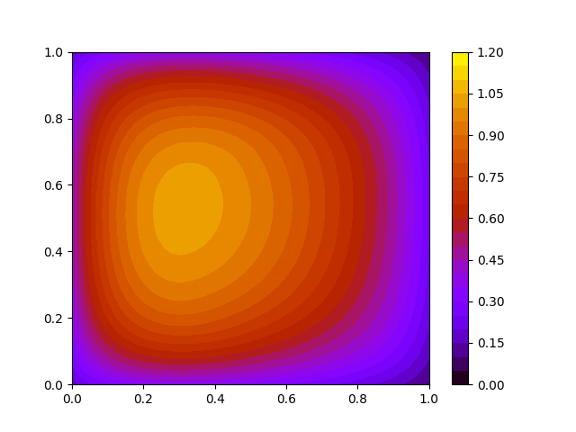
Figure 2: The solution of the direct problem $u(\bm{x},T)$: $u_{\min}=0.0884557$, $u_{\max}=1.03433$

The inverse problem is solved using the fully implicit scheme (see (33)–(35)). The error of the approximate solution of the identification problem on a separate iteration is evaluated as follows:

$$\varepsilon_{\infty}(k)=\max_{\bm{x}\in\Omega}|c^{k}(\bm{x})-c(\bm{x})|,$$

$$\varepsilon_{2}(k)=\|c^{k}(\bm{x})-c(\bm{x})\|.$$

The main issue is to evaluate an actual convergence rate for the iterative processes under the consideration. We need to recognize clearly how quickly the accuracy of the approximate solution is stabilized with increasing the iteration number. The obtained error itself depends on a time step, namely, the smaller time step, the higher accuracy of the approximate solution. Influence of the time step of the iterative process (33)–(35) with the initial approximation (32) on accuracy is shown in Fig. 3. We observe a high convergence of the iterative process and the improvement of the accuracy of the approximate solution by reducing the time step. Similar results for the iterative process with the initial approximation (12) are presented in Fig. 4.

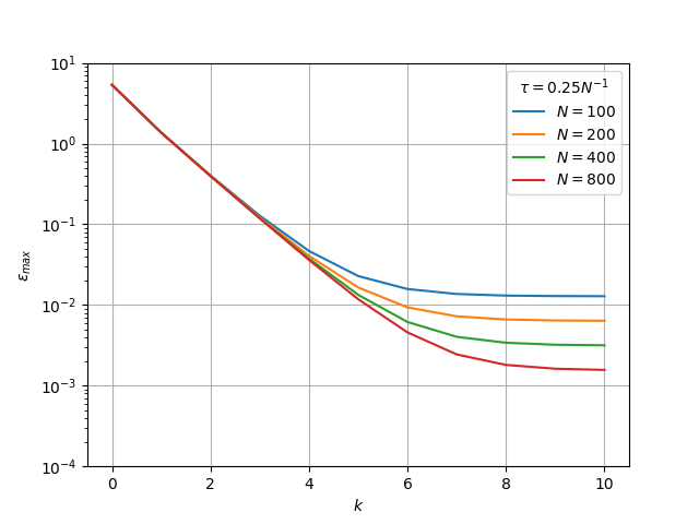
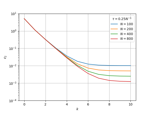
Figure 3: The iterative process with the initial approximation (32)

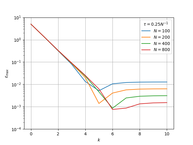
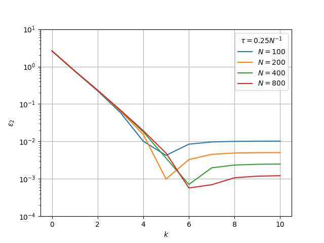
Figure 4: The iterative process with the initial approximation (12)

The convergence of the approximate solution for the reaction coefficient is shown in Fig. 5 and Fig. 6. For the iterative process with initial approximation (32), we observe a monotone convergence from above (see Fig. 5). The iterative process with the initial approximation (12) is non-monotone. In particular, for $k=1$, on a part of the domain $\Omega$, the function $c^{1}({\bm{x}})$ is negative (see Fig. 6).

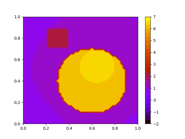
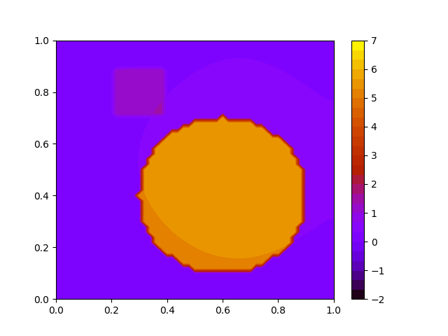
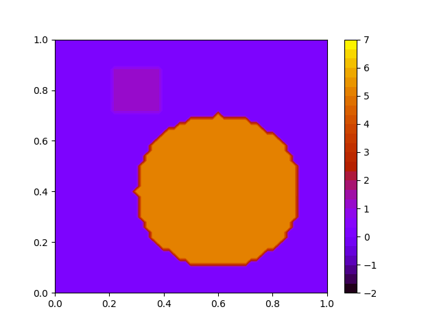
Figure 5: The solution $c({\bm{x}})$ for different $k$ with initial approximation (32): left — $k=1$, center — $k=2$, right — $k=3$

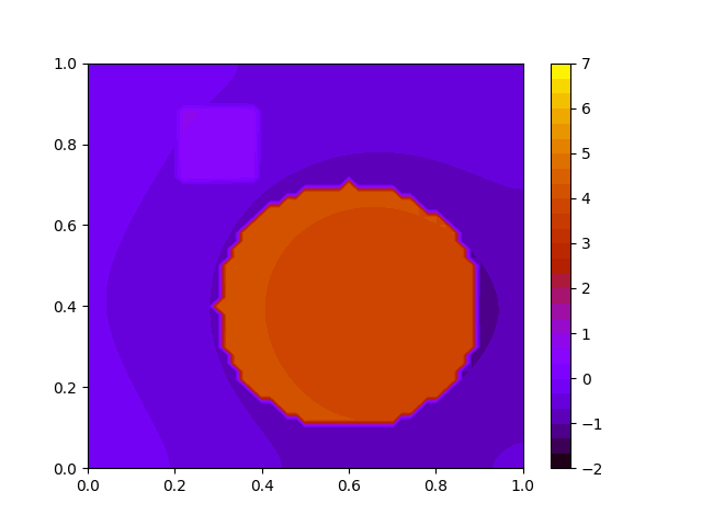
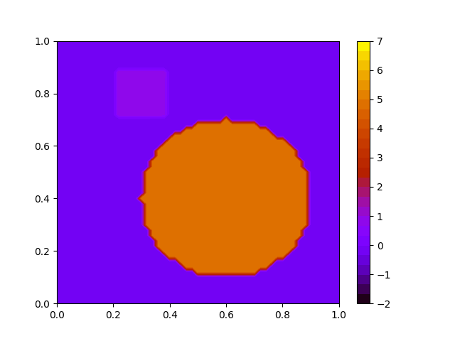
Figure 6: The solution $c({\bm{x}})$ for different $k$ with initial approximation (12): left — $k=1$, center — $k=2$, right — $k=3$

6 Conclusion

1. A nonlinear inverse problem of identifying the lowest coefficient that depends only on spatial variables is studied for a second-order parabolic equation. The solution of the parabolic equation at the final time moment is given, i.e., the final redefinition is considered.

2. An iterative process of identifying an unknown coefficient is conducted by solving the standard initial-boundary value problem at each iteration. The main result is in establishing the monotonicity of the iterative process, where the desired lower coefficient approaches from above.

3. The computational algorithm is based on standard approximations in space by linear finite elements, whereas time-stepping is implemented using the fully implicit two-level schemes.

4. Possibilities of the proposed algorithms were demonstrated by numerical solving a test two-dimensional problem.

References

- Alifanov [2011] O.M. Alifanov, Inverse Heat Transfer Problems, Springer, 2011.
- Brandts et al. [2008] J.H. Brandts, S. Korotov, M. Křížek, The discrete maximum principle for linear simplicial finite element approximations of a reaction–diffusion problem, Linear Algebra and its Applications 429 (2008) 2344–2357.
- Brenner and Scott [2008] S.C. Brenner, L.R. Scott, The Mathematical Theory of Finite Element Methods, Springer, New York, 2008.
- Cao and Lesnic [2018] K. Cao, D. Lesnic, Reconstruction of the space-dependent perfusion coefficient from final time or time-average temperature measurements, Journal of Computational and Applied Mathematics (2018).
- Chatzipantelidis et al. [2015] P. Chatzipantelidis, Z. Horváth, V. Thomée, On preservation of positivity in some finite element methods for the heat equation, Computational Methods in Applied Mathematics 15 (2015) 417–437.
- Chen and Liu [2006] Q. Chen, J. Liu, Solving an inverse parabolic problem by optimization from final measurement data, Journal of Computational and Applied Mathematics 193 (2006) 183–203.
- Ciarlet [1973] P.A. Ciarlet, P. G.and Raviart, Maximum principle and uniform convergence for the finite element method, Computer Methods in Applied Mechanics and Engineering 2 (1973) 17–31.
- Droniou [2014] J. Droniou, Finite volume schemes for diffusion equations: introduction to and review of modern methods, Mathematical Models and Methods in Applied Sciences 24 (2014) 1575–1619.
- Friedman [2008] A. Friedman, Partial Differential Equations of Parabolic Type, Dover, 2008.
- Huang [2011] W. Huang, Discrete maximum principle and a delaunay-type mesh condition for linear finite element approximations of two-dimensional anisotropic diffusion problems, Numerical Mathematics: Theory, Methods and Applications 4 (2011) 319–334.
- Hundsdorfer and Verwer [2003] W.H. Hundsdorfer, J.G. Verwer, Numerical Solution of Time-Dependent Advection-Diffusion-Reaction Equations, Springer Verlag, 2003.
- Il’in et al. [1962] A.M. Il’in, A.S. Kalashnikov, O.A. Oleinik, Linear equations of the second order of parabolic type, Russian Mathematical Surveys 17 (1962) 1–143.
- Isakov [1991] V. Isakov, Inverse parabolic problems with the final overdetermination, Communications on Pure and Applied Mathematics 44 (1991) 185–209.
- Isakov [2017] V. Isakov, Inverse Problems for Partial Differential Equations, 3 ed., Springer, 2017.
- Kamynin [2013] V.L. Kamynin, The inverse problem of determining the lower-order coefficient in parabolic equations with integral observation, Mathematical Notes 94 (2013) 205–213.
- Kamynin and Kostin [2010] V.L. Kamynin, A.B. Kostin, Two inverse problems of finding a coefficient in a parabolic equation, Differential Equations 46 (2010) 375–386.
- Kostin [2015] A.B. Kostin, Inverse problem of finding the coefficient of u in a parabolic equation on the basis of a nonlocal observation condition, Differential Equations 51 (2015) 605–619.
- Lavrent’ev et al. [1986] M.M. Lavrent’ev, V.G. Romanov, S.P. Shishatskii, Ill-posed Problems of Mathematical Physics and Analysis, American Mathematical Society, 1986.
- Letniowski [1992] F.W. Letniowski, Three-dimensional Delaunay triangulations for finite element approximations to a second-order diffusion operator, SIAM Journal on Scientific and Statistical Computing 13 (1992) 765–770.
- Liu [2008] C.S. Liu, An lgsm to identify nonhomogeneous heat conductivity functions by an extra measurement of temperature, International Journal of Heat and Mass Transfer 51 (2008) 2603–2613.
- Liu and Chang [2011] C.S. Liu, C.W. Chang, A lie-group adaptive method to identify the radiative coefficients in parabolic partial differential equations, Computers Materials and Continua 25 (2011) 107.
- Prilepko and Kostin [1992] A.I. Prilepko, A.B. Kostin, Inverse problems of the determination of the coefficient in parabolic equations. I, Siberian Mathematical Journal 33 (1992) 489–496.
- Prilepko and Kostin [1993] A.I. Prilepko, A.B. Kostin, On inverse problems of determining a coefficient in a parabolic equation. II, Siberian Mathematical Journal 34 (1993) 923–937.
- Prilepko et al. [2000] A.I. Prilepko, D.G. Orlovsky, I.A. Vasin, Methods for Solving Inverse Problems in Mathematical Physics, Marcel Dekker, Inc, 2000.
- Prilepko and Solov’ev [1987] A.I. Prilepko, V.V. Solov’ev, On the solvability of inverse boundary value problems for the determination of the coefficient preceding the lower derivative in a parabolic equation, Differentsial’nye Uravneniya 23 (1987) 136–143.
- Samarskii [2001] A.A. Samarskii, The Theory of Difference Schemes, Marcel Dekker, Inc., New York, 2001.
- Samarskii and Vabishchevich [2007] A.A. Samarskii, P.N. Vabishchevich, Numerical Methods for Solving Inverse Problems of Mathematical Physics, De Gruyter, 2007.
- Thomée [2006] V. Thomée, Galerkin Finite Element Methods for Parabolic Problems, Springer Verlag, Berlin, 2006.
- Vabishchevich [2017] P.N. Vabishchevich, Iterative computational identification of a space-wise dependent source in parabolic equation, Inverse Problems in Science and Engineering 25 (2017) 1168–1190.
- Vogel [2002] C.R. Vogel, Computational Methods for Inverse Problems, Society for Industrial and Applied Mathematics, 2002.
- Yang et al. [2008] L. Yang, J.N. Yu, Z.C. Deng, An inverse problem of identifying the coefficient of parabolic equation, Applied Mathematical Modelling 32 (2008) 1984–1995.