Constraining the Polarization Content of Gravitational Waves with Astrometry

Logan O’Beirne eXtreme Gravity Institute, Department of Physics, Montana State University, Bozeman, Montana 59717, USA    Neil J. Cornish eXtreme Gravity Institute, Department of Physics, Montana State University, Bozeman, Montana 59717, USA
Abstract

Gravitational waves perturb the paths of photons, impacting both the time-of-flight and the arrival direction of light from stars. Pulsar timing arrays can detect gravitational waves by measuring the variations in the time of flight of radio pulses, while astrometry missions such as Gaia can detect gravitational waves from the time-varying changes in the apparent position of a field of stars. Just as gravitational waves impart a characteristic correlation pattern in the arrival times of pulses from pulsars at different sky locations, the deflection of starlight is similarly correlated across the sky. Here we compute the astrometric correlation patterns for the full range of polarization states found in alternative theories of gravity, and decompose the sky-averaged correlation patterns into vector spherical harmonics. We find that the tensor and vector polarization states produce equal power in the electric- and magnetic-type vector spherical harmonics, while the scalar modes produce only electric-type correlations. Any difference in the measured electric and magnetic-type correlations would represent a clear violation of Einstein gravity. The angular correlations functions for the vector and scalar longitudinal modes show the same enhanced response at small angular separations that is familiar from pulsar timing.

I Introduction

Gravitational wave astronomy has made it possible to test gravity in the dynamical, strong field regime. The first binary black hole Abbott et al. (2016a) and binary neutron star Abbott et al. (2017a) detections have been used to carry out a wide range of tests, including placing stringent bounds on the difference in propagation speed of gravity and light Cornish et al. (2017a); Abbott et al. (2017b), constraining departures in the waveforms from the predictions of general relativity Abbott et al. (2016b), and constraining the polarization content of the signals Abbott et al. (2017c, d, 2018). The existing array of ground based interferometers is not ideal for testing the polarization content of the signals as the two LIGO detectors and the single Virgo detector provide only a limited number of projections of the polarization. It takes at least 5 (mis-aligned) detectors to unambiguously resolve the polarization content Chatziioannou et al. (2012). The pulsar timing approach to detecting gravitational waves is better suited to measuring polarization Lee et al. (2008); da Silva Alves and Tinto (2011); Chamberlin and Siemens (2012); Cornish et al. (2017b) as each pulsar line-of-sight provides a separate projection of the polarization state. The astrometric approach to detecting gravitational waves Book and Flanagan (2011); Klioner (2018); Moore et al. (2017) is similarly well suited to constraining the polarization content, with astrometric missions such as Gaia Gaia Collaboration et al. (2016) observing billions of stars across the sky.

Photon trajectories are perturbed by gravitational waves, resulting in time delays and changes in the apparent position of the source. Gravitational waves cause the relative position of two stars on the sky to oscillate in a tensor correlation pattern. The formal expression for this tensor two-point correlation pattern, valid for any gravitational wave polarization, was first derived by Book and Flanagan Book and Flanagan (2011), however they only provided explicit expressions for the transverse-tensor modes of general relativity. Here we complete the derivation for the additional four polarization states that are possible in other metric theories of gravity Will (2014); Yunes and Siemens (2013). Book and Flanagan Book and Flanagan (2011) also derived the angular power spectrum, found by expanding the two-point correlation in terms of electric type (E) and magnetic type (B) vector spherical harmonics and integrating over the locations of the stars on the sky. This analysis is analogous to what is done when studying the polarization of the microwave background, where the polarization of the microwave photons are separated into curl-free E-modes and divergence-free B-modes. The tensor-transverse (TT) modes of general relativity produce identical angular correlation patterns for the EE and BB correlations at large angles, and differ slightly at small angular separations (the EB cross correlations vanish for all polarization states) Book and Flanagan (2011). Here we compute the angular power spectra for the additional non-Einsteinian polarization modes. The BB correlation vanishes for the scalar-transverse (ST) and the scalar-longitudinal (SL) polarizations while the EE correlation does not, indicating the the difference in the correlation functions Δ=(EEBB)ΔEEBB\Delta=({\rm EE}-{\rm BB}) provides a powerful null test of general relativity. The vector-longitudinal (VL) polarizations evade this test since they produce identical EE and BB correlation patterns. Both the vector and scalar longitudinal modes produce an enhanced response at small angular separations that depends on the product of the gravitational wave frequency f𝑓f and the distance to the stars L𝐿L. The enhancement is logarithmic for VL and linear for SL. Precisely the same enhancements occur in the two-point correlation functions for these modes for pulsar timing Lee et al. (2008); da Silva Alves and Tinto (2011); Chamberlin and Siemens (2012). This implies that astrometry missions like Gaia will be able to place much stronger constraints on the energy density in the longitudinal modes than for the transverse modes, as is the case for pulsar timing Cornish et al. (2017b).

In the final stages of writing this paper a preprint was posted with an independent calculation of the astrometric two-point correlation functions for non-Einsteinian polarization modes Mihaylov et al. (2018). After accounting for some differences in notation, we verified that our expressions for the two-point functions agree. Their treatment stopped short of computing the E and B mode angular power spectra, and those results are reported here for the first time. We work in geometrical units with G=c=1𝐺𝑐1G=c=1.

II Summary of Results

Our calculation begins with the expression for the astrometric deflection δ𝐧(𝐧,𝐩,t)𝛿𝐧𝐧𝐩𝑡\delta{\bf n}({\bf n},{\bf p},t) for a star in the 𝐧𝐧{\bf n} direction perturbed by a gravitational wave source in the 𝐩𝐩{\bf p} direction. Book and Flanagan Book and Flanagan (2011) provided a formal expression for the deflection that is valid for any gravitational wave polarization. The next step is to compute the two-point correlation function Cij(𝐧,𝐧,f)superscript𝐶𝑖𝑗𝐧superscript𝐧𝑓C^{ij}({\bf n},{\bf n}^{\prime},f) which describe the tensor deflection pattern produced by an isotropic stochastic background of gravitational waves. Book and Flanagan Book and Flanagan (2011) computed a formal expression for Cij(𝐧,𝐧,f)superscript𝐶𝑖𝑗𝐧superscript𝐧𝑓C^{ij}({\bf n},{\bf n}^{\prime},f) that is valid for all polarizations. In practice, to make a detection, we need to combine measurements of the angular deflections between many pairs of stars since the angular deflections between any two stars is expected to be small relative to the noise in the measurement. This is analogous to measurements of the cosmic microwave background, where correlations are computed over large areas of the sky and expressed in terms of angular power spectra. To compute the angular power spectra of the astrometric deflections we decompose the angular deflections into electric-type (E) and magnetic-type (B) vector spherical harmonics and compute the correlations EE,EB,BBEEEBBB{\rm EE,EB,BB} averaged over the distribution of stars in the sky. Assuming a uniform distribution of stars, the correlations only depend on the angle Θ=acos(𝐧𝐧)Θacos𝐧superscript𝐧\Theta={\rm acos}({\bf n}\cdot{\bf n}^{\prime}) between the stars, or equivalently, the multipole moment \ell.

The astrometric deflection δ𝐧(𝐧,𝐩,t)𝛿𝐧𝐧𝐩𝑡\delta{\bf n}({\bf n},{\bf p},t) depends on the phase of the gravitational wave at the Earth and at the star. In the distant source limit, where the product of the gravitational wave frequency f𝑓f and the distance to the star L𝐿L is large, the phase of the star term is uncorrelated between stars located at L𝐧𝐿𝐧L{\bf n} and L𝐧superscript𝐿superscript𝐧L^{\prime}{\bf n}^{\prime} unless Θ0Θ0\Theta\approx 0. For the transverse polarization states the star term can be safely ignored, but not so for the longitudinal modes. The general expression for the two-point correlation function for an isotropic stochastic background can be written as

Cij(𝐧,𝐧,f)=𝑑Ω𝐩δni(𝐧,𝐩,f)δni(𝐧,𝐩,f)superscript𝐶𝑖𝑗𝐧superscript𝐧𝑓differential-dsubscriptΩ𝐩delimited-⟨⟩𝛿superscript𝑛𝑖𝐧𝐩𝑓𝛿superscript𝑛𝑖superscript𝐧𝐩𝑓\displaystyle C^{ij}({\bf n},{\bf n}^{\prime},f)=\int d\Omega_{\bf p}\langle\delta n^{i}({\bf n},{\bf p},f)\delta n^{i}({\bf n}^{\prime},{\bf p},f)\rangle
=3H0232π2Ωgw(f)f3Hij(𝐧,𝐧),absent3superscriptsubscript𝐻0232superscript𝜋2subscriptΩgw𝑓superscript𝑓3superscript𝐻𝑖𝑗𝐧superscript𝐧\displaystyle\quad=\frac{3H_{0}^{2}}{32\pi^{2}}\frac{\Omega_{\rm gw}(f)}{f^{3}}H^{ij}(\mathbf{n},\mathbf{n}^{\prime})\,, (1)

where H0subscript𝐻0H_{0} is the Hubble constant, Ωgw(f)subscriptΩgw𝑓\Omega_{\rm gw}(f) is the energy density in gravitational waves per logarithmic frequency interval, scaled by the critical density ρc=3H02/(8π)subscript𝜌𝑐3superscriptsubscript𝐻028𝜋\rho_{c}=3H_{0}^{2}/(8\pi), Hijsuperscript𝐻𝑖𝑗H^{ij} are the components of the deflection tensor

𝐇(𝐧,𝐧)=α(Θ)(𝐚𝐚)σ(Θ)(𝐛𝐜),𝐇𝐧superscript𝐧𝛼Θtensor-product𝐚𝐚𝜎Θtensor-product𝐛𝐜{\bf H}(\mathbf{n},\mathbf{n}^{\prime})=\alpha(\Theta)({\bf a}\otimes{\bf a})-\sigma(\Theta)({\bf b}\otimes{\bf c}), (2)

and the unit triad 𝐚,𝐛,𝐜𝐚𝐛𝐜{\bf a},{\bf b},{\bf c} is defined by 𝐚=(𝐧×𝐧)/sinΘ𝐚𝐧superscript𝐧Θ{\bf a}=({\bf n}\times{\bf n}^{\prime})/\sin\Theta, 𝐛=(𝐧(𝐧𝐧)𝐧)/sinΘ𝐛𝐧𝐧superscript𝐧superscript𝐧Θ{\bf b}=({\bf n}({\bf n}\cdot{\bf n}^{\prime})-{\bf n}^{\prime})/\sin\Theta, 𝐜=(𝐧(𝐧𝐧)𝐧)/sinΘ𝐜superscript𝐧𝐧superscript𝐧𝐧Θ{\bf c}=({\bf n}^{\prime}({\bf n}\cdot{\bf n}^{\prime})-{\bf n})/\sin\Theta. The angular correlations functions for the tensor transverse (TT), scalar transverse (ST) and vector longitudinal (VL) modes can be computed in closed form in the distant star limit fL𝑓𝐿fL\rightarrow\infty, and are given by

αTT=σTT=(1/12)(7cosΘ5)superscript𝛼TTsuperscript𝜎TT1127cosΘ5\displaystyle\alpha^{\rm TT}=\sigma^{\rm TT}=(1/12)(7\,\text{cos}\,\Theta-5)
8ln(sin(Θ/2))(sin6(Θ/2)/sin2Θ)8lnsinΘ2superscriptsin6Θ2superscriptsin2Θ\displaystyle\hskip 57.81621pt-8\,\text{ln}(\text{sin}(\Theta/2))(\text{sin}^{6}(\Theta/2)/\text{sin}^{2}\Theta)
αST=112superscript𝛼ST112\displaystyle\alpha^{\rm ST}=\frac{1}{12}
σST=112cos(Θ)superscript𝜎ST112cosΘ\displaystyle\sigma^{\rm ST}=\frac{1}{12}\text{cos}(\Theta)
αVL=σVL=sin2(Θ/2)sin2(Θ)[8sin2(Θ/2)ln(sin(Θ/2)\displaystyle\alpha^{\rm VL}=\sigma^{\rm VL}=\frac{\text{sin}^{2}(\Theta/2)}{\text{sin}^{2}(\Theta)}\Big{[}8\,\text{sin}^{2}(\Theta/2)\text{ln}(\text{sin}(\Theta/2)
+13(3+2cos(Θ)cos(2Θ))].\displaystyle\hskip 65.04256pt+\frac{1}{3}\Big{(}3+2\,\text{cos}(\Theta)-\text{cos}(2\Theta)\Big{)}\Big{]}\,. (3)

Plots of the TT, ST and VL correlation patterns are shown in Figure 1.
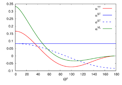
Refer to caption
Figure 1: The analytic correlation functions α(Θ)𝛼Θ\alpha(\Theta) and σ(Θ)𝜎Θ\sigma(\Theta) for the TT, ST and VL modes.

The scalar longitudinal (SL) case is more complicated as the star terms need to be included to arrive at a finite expression at small angular separations. We were unable to derive a closed-form expression for the SL correlation functions that is valid for all angles, and instead quote results that are valid for Θ=0Θ0\Theta=0 and Θ1/(fL)much-greater-thanΘ1𝑓𝐿\Theta\gg 1/(fL). For large angles we have

αSLsin2(Θ/2)3sin2(Θ)[1+cos(Θ)+3ln(sin(Θ/2))]superscript𝛼SLsuperscriptsin2Θ23superscriptsin2Θdelimited-[]1cosΘ3lnsinΘ2\displaystyle\alpha^{\rm SL}\approx-\frac{\text{sin}^{2}(\Theta/2)}{3\,\text{sin}^{2}(\Theta)}\Big{[}1+\text{cos}(\Theta)+3\,\text{ln}(\text{sin}(\Theta/2))\Big{]}
σSLsin2(Θ/2)6sin2(Θ)[4+5cos(Θ)+cos(2Θ)\displaystyle\sigma^{\rm SL}\approx-\frac{\text{sin}^{2}(\Theta/2)}{6\,\text{sin}^{2}(\Theta)}\Big{[}4+5\,\text{cos}(\Theta)+\text{cos}(2\Theta)
+6ln(sin(Θ/2))].\displaystyle\hskip 101.17755pt+6\,\text{ln}(\text{sin}(\Theta/2))\Big{]}\,. (4)

The divergence at Θ=0Θ0\Theta=0 in these expressions is regularized to a logarithmic dependence on the distance to the stars when the star terms are included. To leading order in fL1much-greater-than𝑓𝐿1fL\gg 1 we find

αSL(0)=σSL(0)=18[Φs2Φs24ΦsΦsln(Φs2Φs2)\displaystyle\alpha^{\rm SL}(0)=\sigma^{\rm SL}(0)=\frac{1}{8}\Big{[}\frac{\Phi_{s}^{2}-{\Phi^{\prime}_{s}}^{2}}{4\Phi_{s}\Phi^{\prime}_{s}}\ln(\Phi_{s}^{2}-{\Phi^{\prime}_{s}}^{2})
+ln(ΦsΦs)Φs2+Φs24ΦsΦsln(Φs+Φs)+],\displaystyle\hskip 28.90755pt+\ln(\Phi_{s}\Phi^{\prime}_{s})-\frac{\Phi_{s}^{2}+{\Phi^{\prime}_{s}}^{2}}{4\Phi_{s}\Phi^{\prime}_{s}}\ln(\Phi_{s}+\Phi^{\prime}_{s})+\dots\Big{]}, (5)

where Φs=2πfLsubscriptΦ𝑠2𝜋𝑓𝐿\Phi_{s}=2\pi fL and Φs=2πfLsubscriptsuperscriptΦ𝑠2𝜋𝑓superscript𝐿\Phi^{\prime}_{s}=2\pi fL^{\prime}.

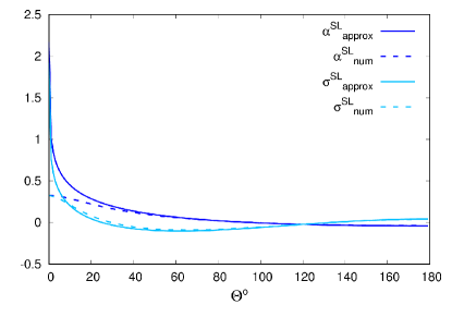
Refer to caption
Figure 2: The correlation functions α(Θ)𝛼Θ\alpha(\Theta) and σ(Θ)𝜎Θ\sigma(\Theta) for the SL mode. The solid lines show the analytic approximation, valid for Θ1/(fL)much-greater-thanΘ1𝑓𝐿\Theta\gg 1/(fL). The dotted lines are found by numerical integration for the case fL=fL=10𝑓𝐿𝑓superscript𝐿10fL=fL^{\prime}=10.

The angular power spectra can be expressed in terms of the multipole coefficients

CmmQQ=d2Ω𝐧d2Ω𝐧YmiQ(𝐧)YmjQ(𝐧)Hij(𝐧,𝐧).subscriptsuperscript𝐶𝑄superscript𝑄𝑚superscriptsuperscript𝑚superscript𝑑2subscriptΩ𝐧superscript𝑑2subscriptΩsuperscript𝐧subscriptsuperscript𝑌𝑄𝑚𝑖𝐧subscriptsuperscript𝑌superscript𝑄superscriptsuperscript𝑚𝑗superscript𝐧subscript𝐻𝑖𝑗𝐧superscript𝐧C^{QQ^{\prime}}_{\ell m\ell^{\prime}m^{\prime}}=\int d^{2}\Omega_{\mathbf{n}}d^{2}\Omega_{\mathbf{n}^{\prime}}Y^{Q*}_{\ell mi}(\mathbf{n})Y^{Q^{\prime}}_{\ell^{\prime}m^{\prime}j}(\mathbf{n}^{\prime})H_{ij}(\mathbf{n},\mathbf{n}^{\prime}). (6)

Here Q,Q𝑄superscript𝑄Q,Q^{\prime} refer to the electric-type and magnetic-type vector spherical harmonics

𝐘lmE(𝐧)=((+1))1/2Ym(𝐧)subscriptsuperscript𝐘𝐸𝑙𝑚𝐧superscript112subscript𝑌𝑚𝐧\displaystyle\mathbf{Y}^{E}_{lm}(\mathbf{n})=(\ell(\ell+1))^{-1/2}\mathbf{\nabla}Y_{\ell m}(\mathbf{n})
𝐘lmB(𝐧)=((+1))1/2(𝐧×)Ym(𝐧)subscriptsuperscript𝐘𝐵𝑙𝑚𝐧superscript112𝐧subscript𝑌𝑚𝐧\displaystyle\mathbf{Y}^{B}_{lm}(\mathbf{n})=(\ell(\ell+1))^{-1/2}(\mathbf{n}\times\mathbf{\nabla})Y_{\ell m}(\mathbf{n}) (7)

The EB cross-correlations vanish due to the different parity of the E and B modes. For an isotropic distribution of stars we find

CmmQQ=δQQδδmm1(+1)4π2+1QQ,subscriptsuperscript𝐶𝑄superscript𝑄𝑚superscriptsuperscript𝑚superscript𝛿𝑄superscript𝑄subscript𝛿superscriptsubscript𝛿𝑚superscript𝑚114𝜋21subscriptQQC^{QQ^{\prime}}_{\ell m\ell^{\prime}m^{\prime}}=\delta^{QQ^{\prime}}\delta_{\ell\ell^{\prime}}\delta_{mm^{\prime}}\frac{1}{\ell(\ell+1)}\frac{4\pi}{2\ell+1}{\rm QQ}_{\ell}\,, (8)

where

QQ=𝑑ΘP(cosΘ)QQ(Θ).subscriptQQdifferential-dΘsubscript𝑃ΘQQΘ{\rm QQ}_{\ell}=\int d\Theta\,P_{\ell}(\cos\Theta){\rm QQ}(\Theta)\,. (9)

The formal expressions for the EE and BB correlation functions are:

EE(Θ)=ij[Hij(𝐧,𝐧)]EEΘsubscript𝑖subscriptsuperscript𝑗superscript𝐻𝑖𝑗𝐧superscript𝐧\displaystyle{\rm EE}(\Theta)=\nabla_{i}\nabla^{\prime}_{j}\left[H^{ij}(\mathbf{n},\mathbf{n}^{\prime})\right]
BB(Θ)=lp[ϵiklϵjmpnknmHij(𝐧,𝐧)].BBΘsuperscript𝑙superscriptsuperscript𝑝subscriptitalic-ϵ𝑖𝑘𝑙subscriptitalic-ϵ𝑗𝑚𝑝superscript𝑛𝑘superscriptsuperscript𝑛𝑚superscript𝐻𝑖𝑗𝐧superscript𝐧\displaystyle{\rm BB}(\Theta)=\nabla^{l}{\nabla^{\prime}}^{p}\left[\epsilon_{ikl}\epsilon_{jmp}n^{k}{n^{\prime}}^{m}H^{ij}(\mathbf{n},\mathbf{n}^{\prime})\right]. (10)

Note that EE(Θ)EEΘ{\rm EE}(\Theta) and BB(Θ)BBΘ{\rm BB}(\Theta), or equivalently EEsubscriptEE{\rm EE}_{\ell} and BBsubscriptBB{\rm BB}_{\ell}, are physical observables that can be inferred from astrometric data, just as the EE and BB power spectra for the CMB polarization are physical observables. A method for extracting CmmQQsubscriptsuperscript𝐶𝑄superscript𝑄𝑚superscriptsuperscript𝑚C^{QQ^{\prime}}_{\ell m\ell^{\prime}m^{\prime}}, and hence EEsubscriptEE{\rm EE}_{\ell} and BBsubscriptBB{\rm BB}_{\ell}, from Gaia observations is described in Ref. Mignard and Klioner (2012).
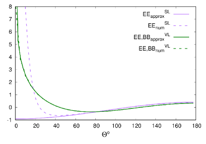
Refer to caption
Figure 3: The upper plot shows EE and BB angular correlation functions for the longitudinal modes. The solid lines are the analytic approximations from Eq. (II) and the dotted lines are from a numerical evaluation with fL=10𝑓𝐿10fL=10.

At large angles we find that EE(Θ)=BB(Θ)EEΘBBΘ{\rm EE}(\Theta)={\rm BB}(\Theta) for the TT and VL modes, and for the scalar modes ST and SL we find BB(Θ)=0BBΘ0{\rm BB}(\Theta)=0, as expected from the even parity of the scalar perturbations. Additional care must be taken when computing the angular power spectra as the derivatives acting on Hij(𝐧,𝐧)subscript𝐻𝑖𝑗𝐧superscript𝐧H_{ij}(\mathbf{n},\mathbf{n}^{\prime}) act on the phase of the star term, and modify the behavior at small angles. In the distant star limit we find

EETT(Θ)=23[2(1cosΘ2)\displaystyle{\rm EE}^{\rm TT}(\Theta)=\frac{2}{3}\Big{[}2-\Big{(}\frac{1-\text{cos}\Theta}{2}\Big{)}
+6(1cosΘ2)ln(1cosΘ2)]\displaystyle\hskip 57.81621pt+6\,\Big{(}\frac{1-\text{cos}\Theta}{2}\Big{)}\text{ln}\Big{(}\frac{1-\text{cos}\Theta}{2}\Big{)}\Big{]}
BBTT(Θ)=EETT(Θ)superscriptBBTTΘsuperscriptEETTΘ\displaystyle{\rm BB}^{\rm TT}(\Theta)={\rm EE}^{\rm TT}(\Theta)
EEVL(Θ)13(3+4cos(Θ)+6ln(sin(Θ/2)))superscriptEEVLΘ1334cosΘ6lnsinΘ2\displaystyle{\rm EE}^{\rm VL}(\Theta)\approx-\frac{1}{3}\Big{(}3+4\,\text{cos}(\Theta)+6\,\text{ln}(\text{sin}(\Theta/2))\Big{)}
BBVL(Θ)=EEVL(Θ)superscriptBBVLΘsuperscriptEEVLΘ\displaystyle{\rm BB}^{\rm VL}(\Theta)={\rm EE}^{\rm VL}(\Theta)
BBST(Θ)=BBSL(Θ)=0superscriptBBSTΘsuperscriptBBSLΘ0\displaystyle{\rm BB}^{\rm ST}(\Theta)={\rm BB}^{\rm SL}(\Theta)=0
EEST(Θ)=13cosΘsuperscriptEESTΘ13cosΘ\displaystyle{\rm EE}^{\rm ST}(\Theta)=\frac{1}{3}\,\text{cos}\Theta
EESL(Θ)112(3+8cosΘ),superscriptEESLΘ11238cosΘ\displaystyle{\rm EE}^{\rm SL}(\Theta)\approx-\frac{1}{12}(3+8\,\text{cos}\,\Theta), (11)

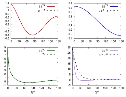
Note that up to an overall scaling, the correlation pattern for the TT mode is identical to the Hellings-Downs curve from pulsar timing. Similarly, the EE correlation for the ST mode has the same form as the ST correlation function from pulsar timing, aside from an overall constant offset and scaling. The expressions for the scalar longitudinal and vector longitudinal modes are only valid for Θ1/(fL)much-greater-thanΘ1𝑓𝐿\Theta\gg 1/(fL). Derivatives of the star terms become important at small angular separations. A complete numerical treatment would need to integrate over the radial distribution of stars, but to simplify the calculation we will assume that all the stars are at the same distance. Figure 3 compares the closed-form approximations to the correlation functions for the longitudinal modes to the numerical evaluation with fL=10𝑓𝐿10fL=10.

Refer to caption
Figure 4: The EE angular correlation functions are compared to the corresponding correlation functions ΓΓ\Gamma for pulsar timing. Aside from overall scalings and offsets, the correlation functions for the transverse modes are identical. The vector longitudinal correlation functions are identical at large angles, but differ slightly at small angles, though both share a similar ln(fL)𝑓𝐿\ln(fL) scaling at Θ=0Θ0\Theta=0 . The correlation functions for the scalar longitudinal modes are qualitatively similar, but differ in their detailed form. They share a similar fL𝑓𝐿fL dependent scaling at Θ=0Θ0\Theta=0. The plots are shown for fL=10𝑓𝐿10fL=10.

The derivatives of Hij(𝐧,𝐧)subscript𝐻𝑖𝑗𝐧superscript𝐧H_{ij}(\mathbf{n},\mathbf{n}^{\prime}) that appear in the definition of the EE and BB correlation functions enhance the importance of the star terms at small angular separations and produce an enhanced response. For the VL modes we find that the enhancement at Θ=0Θ0\Theta=0 scales as ln(fL)𝑓𝐿\ln(fL), while for the SL mode we find that the enhancement scales as fL𝑓𝐿fL. These enhancement factors are identical to those found for the VL and SL angular correlation functions for pulsar timing. This implies that astrometric observatories such as Gaia will be able to place much tighter constraints on the energy density of the longitudinal modes, as is the case for pulsar timing Cornish et al. (2017b). Figure 4 compares the numerically computed EE correlation functions to the corresponding two-point angular correlation functions ΓΓ\Gamma for pulsar timing  Lee et al. (2008). Aside from an overall difference in scaling and a constant shift for the scalar mode, the correlation functions for the transverse modes are identical for astrometry and pulsar timing. The vector longitudinal correlation functions are identical at large angles, but differ slightly at small angles, though both scale as ln(fL)𝑓𝐿\ln(fL) at small angles, albeit with different scaling coefficients. The correlation functions for the scalar longitudinal modes are qualitatively similar, but differ in their detailed form. They both scale as fL𝑓𝐿fL for small angles, but with different scaling coefficients.

III Computing the two-point correlation functions

The angular deflection of a star at location 𝐍=𝐧L𝐍𝐧𝐿{\bf N}={\bf n}L caused by a plane gravitational wave hij(t,x)=[ije2πif(t𝐩𝐱)]subscript𝑖𝑗𝑡xsubscript𝑖𝑗superscript𝑒2𝜋𝑖𝑓𝑡𝐩𝐱h_{ij}(t,\textbf{x})=\Re[\mathcal{H}_{ij}e^{-2\pi if(t-{\bf p}\cdot{\bf x})}] propagating in the 𝐩𝐩{\bf p} direction is given by Book and Flanagan (2011)

δni(𝐧,𝐩,t)=[ikl(n,p)kle2πift]𝛿superscript𝑛𝑖𝐧𝐩𝑡superscript𝑖𝑘𝑙npsubscript𝑘𝑙superscripte2𝜋𝑖𝑓𝑡\delta n^{i}({\bf n},{\bf p},t)=\Re\Big{[}\mathcal{R}^{ikl}(\textbf{n},\textbf{p})\mathcal{H}_{kl}\text{e}^{-2\pi ift}\Big{]} (12)

where

ikl(n,p)=12[(Tn1ni+Tppi)nknl1+pnTn2nkδil]superscript𝑖𝑘𝑙np12delimited-[]subscript𝑇subscriptn1superscript𝑛𝑖subscript𝑇psuperscript𝑝𝑖superscript𝑛𝑘superscript𝑛𝑙1pnsubscript𝑇subscriptn2superscript𝑛𝑘superscript𝛿𝑖𝑙\mathcal{R}^{ikl}(\textbf{n},\textbf{p})=\frac{1}{2}\Big{[}\frac{(T_{\textbf{n}_{1}}\,n^{i}+T_{\textbf{p}}\,p^{i})\,n^{k}\,n^{l}}{1+\textbf{p}\cdot\textbf{n}}-T_{\textbf{n}_{2}}\,n^{k}\delta^{il}\Big{]} (13)

and

Tn1=1i(2+𝐩𝐧)Φs(1+𝐩𝐧)eiΦs(1+𝐩𝐧)subscript𝑇subscriptn11𝑖2𝐩𝐧subscriptΦ𝑠1𝐩𝐧superscript𝑒𝑖subscriptΦ𝑠1𝐩𝐧\displaystyle T_{\textbf{n}_{1}}=1-\frac{i(2+{\bf p}\cdot{\bf n})}{\Phi_{s}(1+{\bf p}\cdot{\bf n})}e^{i\Phi_{s}(1+{\bf p}\cdot{\bf n})}
Tp=1iΦs(1+𝐩𝐧)eiΦs(1+𝐩𝐧))\displaystyle T_{\textbf{p}}=1-\frac{i}{\Phi_{s}(1+{\bf p}\cdot{\bf n})}e^{i\Phi_{s}(1+{\bf p}\cdot{\bf n})})
Tn2=12iΦs(1+𝐩𝐧)eiΦs(1+𝐩𝐧)subscript𝑇subscriptn212𝑖subscriptΦ𝑠1𝐩𝐧superscript𝑒𝑖subscriptΦ𝑠1𝐩𝐧\displaystyle T_{\textbf{n}_{2}}=\frac{1}{2}-\frac{i}{\Phi_{s}(1+{\bf p}\cdot{\bf n})}e^{i\Phi_{s}(1+{\bf p}\cdot{\bf n})} (14)

with Φs=2πfLsubscriptΦ𝑠2𝜋𝑓𝐿\Phi_{s}=2\pi fL. To compute the two-point correlation function Cij(𝐧,𝐧,f)superscript𝐶𝑖𝑗𝐧superscript𝐧𝑓C^{ij}({\bf n},{\bf n}^{\prime},f) we define the orthonormal coordinate system (𝐦,𝐥,𝐧)𝐦𝐥𝐧({\bf m},{\bf l},{\bf n}) and introduce the gravitational wave polarization tetrad (𝐮,𝐯,𝐩)𝐮𝐯𝐩({\bf u},{\bf v},{\bf p}):

𝐩=cosθ𝐧+sinθ(cosϕ𝐦+sinϕ𝐥),𝐩𝜃𝐧𝜃italic-ϕ𝐦italic-ϕ𝐥\displaystyle{\bf p}=\cos\theta\,{\bf n}+\sin\theta(\cos\phi\,{\bf m}+\sin\phi\,{\bf l}),
𝐮=(sinθcosϕ𝐧+cosθ𝐦)sin2θcos2ϕ+cos2θ,𝐮𝜃italic-ϕ𝐧𝜃𝐦superscript2𝜃superscript2italic-ϕsuperscript2𝜃\displaystyle{\bf u}=\frac{\left(-\sin\theta\cos\phi\,{\bf n}+\cos\theta\,{\bf m}\right)}{\sqrt{\sin^{2}\theta\cos^{2}\phi+\cos^{2}\theta}},
𝐯=(sinθcosθsinϕ𝐧+sin2θcosϕsinϕ𝐦)sin2θcos2ϕ+cos2θ𝐯𝜃𝜃italic-ϕ𝐧superscript2𝜃italic-ϕitalic-ϕ𝐦superscript2𝜃superscript2italic-ϕsuperscript2𝜃\displaystyle{\bf v}=-\frac{\left(\sin\theta\cos\theta\sin\phi\,{\bf n}+\sin^{2}\theta\cos\phi\sin\phi\,{\bf m}\right)}{\sqrt{\sin^{2}\theta\cos^{2}\phi+\cos^{2}\theta}}
+(sin2θcos2ϕ+cos2θ)𝐥sin2θcos2ϕ+cos2θsuperscript2𝜃superscript2italic-ϕsuperscript2𝜃𝐥superscript2𝜃superscript2italic-ϕsuperscript2𝜃\displaystyle\hskip 28.90755pt+\frac{(\sin^{2}\theta\cos^{2}\phi+\cos^{2}\theta)\,{\bf l}}{\sqrt{\sin^{2}\theta\cos^{2}\phi+\cos^{2}\theta}} (15)

The basis tensors for the various gravitational wave polarization states are then

ϵTT+=𝐮𝐮𝐯𝐯subscriptsuperscriptbold-italic-ϵTTtensor-product𝐮𝐮tensor-product𝐯𝐯\displaystyle\boldsymbol{\epsilon}^{+}_{\rm TT}={\bf u}\otimes{\bf u}-{\bf v}\otimes{\bf v}
ϵTT×=𝐮𝐯+𝐯𝐮subscriptsuperscriptbold-italic-ϵTTtensor-product𝐮𝐯tensor-product𝐯𝐮\displaystyle\boldsymbol{\epsilon}^{\times}_{\rm TT}={\bf u}\otimes{\bf v}+{\bf v}\otimes{\bf u}
ϵST=𝐮𝐮+𝐯𝐯subscriptsuperscriptbold-italic-ϵdirect-productSTtensor-product𝐮𝐮tensor-product𝐯𝐯\displaystyle\boldsymbol{\epsilon}^{\odot}_{\rm ST}={\bf u}\otimes{\bf u}+{\bf v}\otimes{\bf v}
ϵVLu=𝐮𝐩+𝐩𝐮subscriptsuperscriptbold-italic-ϵ𝑢VLtensor-product𝐮𝐩tensor-product𝐩𝐮\displaystyle\boldsymbol{\epsilon}^{u}_{{\rm VL}}={\bf u}\otimes{\bf p}+{\bf p}\otimes{\bf u}
ϵVLv=𝐯𝐩+𝐩𝐯subscriptsuperscriptbold-italic-ϵ𝑣VLtensor-product𝐯𝐩tensor-product𝐩𝐯\displaystyle\boldsymbol{\epsilon}^{v}_{{\rm VL}}={\bf v}\otimes{\bf p}+{\bf p}\otimes{\bf v}
ϵSL=𝐩𝐩.subscriptsuperscriptbold-italic-ϵdirect-productSLtensor-product𝐩𝐩\displaystyle\boldsymbol{\epsilon}^{\odot}_{{\rm SL}}={\bf p}\otimes{\bf p}\,. (16)

The 𝐧superscript𝐧{\bf n}^{\prime} vector can be written as

𝐧=cosΘ𝐧+sinΘ(cosΦ𝐦+sinΦ𝐥).superscript𝐧Θ𝐧ΘΦ𝐦Φ𝐥{\bf n}^{\prime}=\cos\Theta\,{\bf n}+\sin\Theta(\cos\Phi\,{\bf m}+\sin\Phi\,{\bf l})\,. (17)

The two-point correlation function Cij(𝐧,𝐧,f)superscript𝐶𝑖𝑗𝐧superscript𝐧𝑓C^{ij}({\bf n},{\bf n}^{\prime},f) can be written in terms of the tensor Hij(𝐧,𝐧)=α(Θ)aiajσ(Θ)bicjsuperscript𝐻𝑖𝑗𝐧superscript𝐧𝛼Θsuperscript𝑎𝑖superscript𝑎𝑗𝜎Θsuperscript𝑏𝑖superscript𝑐𝑗H^{ij}(\mathbf{n},\mathbf{n}^{\prime})=\alpha(\Theta)a^{i}a^{j}-\sigma(\Theta)b^{i}c^{j}. Written in the the (𝐦,𝐥,𝐧)𝐦𝐥𝐧({\bf m},{\bf l},{\bf n}) coordinate system we have

𝐚=(sinΦ𝐦+cosΦ𝐥)𝐚Φ𝐦Φ𝐥\displaystyle{\bf a}=(-\sin\Phi\,{\bf m}+\cos\Phi\,{\bf l})
𝐛=(cosΦ𝐦+sinΦ𝐥)𝐛Φ𝐦Φ𝐥\displaystyle{\bf b}=-(\cos\Phi\,{\bf m}+\sin\Phi\,{\bf l})
𝐜=sinΘ𝐧+cosΘ(sinΦ𝐦+cosΦ𝐥).𝐜Θ𝐧ΘΦ𝐦Φ𝐥\displaystyle{\bf c}=-\sin\Theta\,{\bf n}+\cos\Theta(\sin\Phi\,{\bf m}+\cos\Phi\,{\bf l})\,. (18)

The angular correlation functions are given by

αP(Θ)=14πsin2(Θ)d2Ω𝐩aiikl(n,p)ϵklP(p)superscript𝛼𝑃Θ14𝜋superscriptsin2Θsuperscript𝑑2subscriptΩ𝐩superscript𝑎𝑖subscript𝑖𝑘𝑙npsubscriptsuperscriptitalic-ϵ𝑃𝑘𝑙p\displaystyle\alpha^{P}(\Theta)=\frac{1}{4\pi\,\text{sin}^{2}(\Theta)}\int d^{2}\Omega_{\bf p}a^{i}\mathcal{R}_{ikl}(\textbf{n},\textbf{p})\,\epsilon^{P}_{kl}(\textbf{p})
×ajjrs(n,p)ϵrsP(p)absentsuperscript𝑎𝑗subscript𝑗𝑟𝑠superscriptsuperscriptnpsubscriptsuperscriptitalic-ϵ𝑃𝑟𝑠p\displaystyle\hskip 86.72377pt\times\,a^{j}\mathcal{R}_{jrs}(\textbf{n}^{\prime},\textbf{p})^{*}\,\epsilon^{P}_{rs}(\textbf{p})
σP(Θ)=14πsin2(Θ)d2Ω𝐩biikl(n,p)ϵklP(p)superscript𝜎𝑃Θ14𝜋superscriptsin2Θsuperscript𝑑2subscriptΩ𝐩superscript𝑏𝑖subscript𝑖𝑘𝑙npsubscriptsuperscriptitalic-ϵ𝑃𝑘𝑙p\displaystyle\sigma^{P}(\Theta)=-\frac{1}{4\pi\,\text{sin}^{2}(\Theta)}\int d^{2}\Omega_{\bf p}b^{i}\mathcal{R}_{ikl}(\textbf{n},\textbf{p})\,\epsilon^{P}_{kl}(\textbf{p})
×cjjrs(n,p)ϵrsP(p)absentsuperscript𝑐𝑗subscript𝑗𝑟𝑠superscriptsuperscriptnpsubscriptsuperscriptitalic-ϵ𝑃𝑟𝑠p\displaystyle\hskip 86.72377pt\times\,c^{j}\mathcal{R}_{jrs}(\textbf{n}^{\prime},\textbf{p})^{*}\,\epsilon^{P}_{rs}(\textbf{p}) (19)

where d2Ω𝐩=sinθdθdϕsuperscript𝑑2subscriptΩ𝐩𝜃𝑑𝜃𝑑italic-ϕd^{2}\Omega_{\mathbf{p}}=\sin\theta\,d\theta d\phi . The correlation functions for the TT and VL modes are defined as being summed over the +,×+,\times or u,v𝑢𝑣u,v states. The correlation functions for ST and SL only have a single contribution. The full expression for the correlation functions are lengthy. To render the expressions manageable we follow Ref. Book and Flanagan (2011) and introduce the quantities κ=𝐧𝐩𝜅𝐧𝐩\kappa=\mathbf{n}\cdot\mathbf{p}, κ=𝐧𝐩superscript𝜅superscript𝐧𝐩\kappa^{\prime}=\mathbf{n}^{\prime}\cdot\mathbf{p}, λ=𝐧𝐧𝜆𝐧superscript𝐧\lambda=\mathbf{n}\cdot\mathbf{n}^{\prime}, ν2=1κ2superscript𝜈21superscript𝜅2\nu^{2}=1-\kappa^{2}, ν2=1κ2superscript𝜈21superscript𝜅2\nu^{\prime 2}=1-\kappa^{\prime 2}, μ=sinΘ𝐚𝐩𝜇Θ𝐚𝐩\mu=\sin\Theta\,\mathbf{a}\cdot\mathbf{p}, which satisfy the identity 1+2λκκ=μ2+λ2+κ2+κ212𝜆𝜅superscript𝜅superscript𝜇2superscript𝜆2superscript𝜅2superscript𝜅21+2\lambda\kappa\kappa^{\prime}=\mu^{2}+\lambda^{2}+\kappa^{2}+\kappa^{\prime 2}. The correlation functions are then given by

αTT(Θ)=116πsin2(Θ)d2Ω𝐩[μ2(ν2ν22μ2)(1+κ)(1+κ)TpTp\displaystyle\alpha^{\rm TT}(\Theta)=\frac{1}{16\pi\sin^{2}(\Theta)}\int d^{2}\Omega_{\mathbf{p}}\Big{[}\frac{\mu^{2}(\nu^{2}\nu^{\prime 2}-2\mu^{2})}{(1+\kappa)(1+\kappa^{\prime})}T_{\textbf{p}}T_{\textbf{p}^{\prime}}^{*}
μ2(κκ22λκ+κ)(1+κ)TpTn2superscript𝜇2superscript𝜅superscript𝜅22𝜆𝜅superscript𝜅1𝜅subscript𝑇psuperscriptsubscript𝑇superscriptsubscriptn2\displaystyle\hskip 79.49744pt-\frac{\mu^{2}(\kappa^{\prime}\kappa^{2}-2\lambda\kappa+\kappa^{\prime})}{(1+\kappa)}T_{\textbf{p}}T_{\textbf{n}_{2}^{\prime}}^{*}
μ2(κκ22λκ+κ)(1+κ)Tn2Tpsuperscript𝜇2𝜅superscript𝜅22𝜆superscript𝜅𝜅1superscript𝜅subscript𝑇subscriptn2superscriptsubscript𝑇superscriptp\displaystyle\hskip 79.49744pt-\frac{\mu^{2}(\kappa\kappa^{\prime 2}-2\lambda\kappa^{\prime}+\kappa)}{(1+\kappa^{\prime})}T_{\textbf{n}_{2}}T_{\textbf{p}^{\prime}}^{*}
+(λκκ)(1λ2μ2)Tn2Tn2]\displaystyle\hskip 72.26999pt+(\lambda-\kappa\kappa^{\prime})(1-\lambda^{2}-\mu^{2})T_{\textbf{n}_{2}}T_{\textbf{n}_{2}^{\prime}}^{*}\Big{]} (20)
σTT(Θ)=116πsin2(Θ)d2Ω𝐩×\displaystyle\sigma^{\rm TT}(\Theta)=-\frac{1}{16\pi\sin^{2}(\Theta)}\int d^{2}\Omega_{\mathbf{p}}\times
[(λκκ)(λκκ)(ν2ν22μ2)(1+κ)(1+κ)TpTp\displaystyle\hskip 21.68121pt\Big{[}\frac{(\lambda\kappa-\kappa^{\prime})(\lambda\kappa^{\prime}-\kappa)(\nu^{2}\nu^{\prime 2}-2\mu^{2})}{(1+\kappa)(1+\kappa^{\prime})}T_{\textbf{p}}T_{\textbf{p}^{\prime}}^{*}
(λκκ)[λ(ν2ν22μ2)ν2(λκκ)](1+κ)TpTn2𝜆𝜅superscript𝜅delimited-[]𝜆superscript𝜈2superscript𝜈22superscript𝜇2superscript𝜈2𝜆𝜅superscript𝜅1𝜅subscript𝑇psuperscriptsubscript𝑇superscriptsubscriptn2\displaystyle-\frac{(\lambda\kappa-\kappa^{\prime})[\lambda(\nu^{2}\nu^{\prime 2}-2\mu^{2})-\nu^{2}(\lambda-\kappa\kappa^{\prime})]}{(1+\kappa)}T_{\textbf{p}}T_{\textbf{n}_{2}^{\prime}}^{*}
(λκκ)[λ(ν2ν22μ2)ν2(λκκ)](1+κ)Tn2Tp𝜆superscript𝜅𝜅delimited-[]𝜆superscript𝜈2superscript𝜈22superscript𝜇2superscript𝜈2𝜆𝜅superscript𝜅1superscript𝜅subscript𝑇subscriptn2superscriptsubscript𝑇superscriptp\displaystyle-\frac{(\lambda\kappa^{\prime}-\kappa)[\lambda(\nu^{2}\nu^{\prime 2}-2\mu^{2})-\nu^{\prime 2}(\lambda-\kappa\kappa^{\prime})]}{(1+\kappa^{\prime})}T_{\textbf{n}_{2}}T_{\textbf{p}^{\prime}}^{*}
+[λ2(ν2ν22μ2ν2ν2)\displaystyle\hskip 43.36243pt+[\lambda^{2}(\nu^{2}\nu^{\prime 2}-2\mu^{2}-\nu^{2}-\nu^{\prime 2})
+λκκ(ν2+ν2)+ν2ν2]Tn2Tn2]\displaystyle\hskip 57.81621pt+\lambda\kappa\kappa^{\prime}(\nu^{2}+\nu^{\prime 2})+\nu^{2}\nu^{\prime 2}]T_{\textbf{n}_{2}}T_{\textbf{n}_{2}^{\prime}}^{*}\Big{]} (21)
αST(Θ)=116πsin2(Θ)d2Ω𝐩[μ2(1κ)(1κ)TpTp\displaystyle\alpha^{\rm ST}(\Theta)=\frac{1}{16\pi\sin^{2}(\Theta)}\int d^{2}\Omega_{\mathbf{p}}\Big{[}\mu^{2}(1-\kappa)(1-\kappa^{\prime})T_{\textbf{p}}T_{\textbf{p}^{\prime}}^{*}
+μ2κ(1κ)TpTn2+μ2κ(1κ)Tn2Tpsuperscript𝜇2superscript𝜅1𝜅subscript𝑇psuperscriptsubscript𝑇superscriptsubscriptn2superscript𝜇2𝜅1superscript𝜅subscript𝑇subscriptn2superscriptsubscript𝑇superscriptp\displaystyle\hskip 50.58878pt+\mu^{2}\kappa^{\prime}(1-\kappa)T_{\textbf{p}}T_{\textbf{n}_{2}^{\prime}}^{*}+\mu^{2}\kappa(1-\kappa^{\prime})T_{\textbf{n}_{2}}T_{\textbf{p}^{\prime}}^{*}
+(μ2κκ)Tn2Tn2]\displaystyle\hskip 130.08621pt+(\mu^{2}\kappa\kappa^{\prime})T_{\textbf{n}_{2}}T_{\textbf{n}_{2}^{\prime}}^{*}\Big{]} (22)
σST(Θ)=116πsin2(Θ)d2Ω𝐩×\displaystyle\sigma^{\rm ST}(\Theta)=-\frac{1}{16\pi\sin^{2}(\Theta)}\int d^{2}\Omega_{\mathbf{p}}\times
[(λκκ)(λκκ)(1κ)(1κ)TpTp\displaystyle\hskip 14.45377pt\Big{[}(\lambda\kappa-\kappa^{\prime})(\lambda\kappa^{\prime}-\kappa)(1-\kappa)(1-\kappa^{\prime})T_{\textbf{p}}T_{\textbf{p}^{\prime}}^{*}
+(λκκ)(λκκ)(1κ)κTpTn2𝜆𝜅superscript𝜅𝜆superscript𝜅𝜅1𝜅superscript𝜅subscript𝑇psuperscriptsubscript𝑇superscriptsubscriptn2\displaystyle\hskip 36.135pt+(\lambda\kappa-\kappa^{\prime})(\lambda\kappa^{\prime}-\kappa)(1-\kappa)\kappa^{\prime}T_{\textbf{p}}T_{\textbf{n}_{2}^{\prime}}^{*}
+(λκκ)(λκκ)(1κ)κTn2Tp𝜆𝜅superscript𝜅𝜆superscript𝜅𝜅1superscript𝜅𝜅subscript𝑇subscriptn2superscriptsubscript𝑇superscriptp\displaystyle\hskip 36.135pt+(\lambda\kappa-\kappa^{\prime})(\lambda\kappa^{\prime}-\kappa)(1-\kappa^{\prime})\kappa T_{\textbf{n}_{2}}T_{\textbf{p}^{\prime}}^{*}
+[λ2ν2ν2λ(λκκ)(ν2+ν2)\displaystyle\hskip 57.81621pt+[\lambda^{2}\nu^{2}\nu^{\prime 2}-\lambda(\lambda-\kappa\kappa^{\prime})(\nu^{2}+\nu^{\prime 2})
+(λκκ)2]Tn2Tn2]\displaystyle\hskip 115.63243pt+(\lambda-\kappa\kappa^{\prime})^{2}]T_{\textbf{n}_{2}}T_{\textbf{n}_{2}^{\prime}}^{*}\Big{]} (23)
αVL(Θ)=116πsin2(Θ)d2Ω𝐩4μ2κκ(λκκ)(1+κ)(1+κ)TpTpsuperscript𝛼VLΘ116𝜋superscript2Θsuperscript𝑑2subscriptΩ𝐩4superscript𝜇2𝜅superscript𝜅𝜆𝜅superscript𝜅1𝜅1superscript𝜅subscript𝑇psuperscriptsubscript𝑇superscriptp\displaystyle\alpha^{\rm VL}(\Theta)=\frac{1}{16\pi\sin^{2}(\Theta)}\int d^{2}\Omega_{\mathbf{p}}\frac{4\mu^{2}\kappa\kappa^{\prime}(\lambda-\kappa\kappa^{\prime})}{(1+\kappa)(1+\kappa^{\prime})}T_{\textbf{p}}T_{\textbf{p}^{\prime}}^{*}
2μ2κ(λ2κκ)(1+κ)TpTn22μ2κ(λ2κκ)(1+κ)Tn2Tp2superscript𝜇2𝜅𝜆2𝜅superscript𝜅1𝜅subscript𝑇psuperscriptsubscript𝑇superscriptsubscriptn22superscript𝜇2superscript𝜅𝜆2𝜅superscript𝜅1superscript𝜅subscript𝑇subscriptn2superscriptsubscript𝑇superscriptp\displaystyle-\frac{2\mu^{2}\kappa(\lambda-2\kappa\kappa^{\prime})}{(1+\kappa)}T_{\textbf{p}}T_{\textbf{n}_{2}^{\prime}}^{*}-\frac{2\mu^{2}\kappa^{\prime}(\lambda-2\kappa\kappa^{\prime})}{(1+\kappa^{\prime})}T_{\textbf{n}_{2}}T_{\textbf{p}^{\prime}}^{*}
+[λμ2κκ(4μ2+λ21)]Tn2Tn2]\displaystyle\hskip 50.58878pt+[\lambda\mu^{2}-\kappa\kappa^{\prime}(4\mu^{2}+\lambda^{2}-1)]T_{\textbf{n}_{2}}T_{\textbf{n}_{2}^{\prime}}^{*}\Big{]} (24)
σVL(Θ)=116πsin2(Θ)d2Ω𝐩×\displaystyle\sigma^{\rm VL}(\Theta)=-\frac{1}{16\pi\sin^{2}(\Theta)}\int d^{2}\Omega_{\mathbf{p}}\times
[4(λκκ)(λκκ)κκ(λκκ)(1+κ)(1+κ)TpTp\displaystyle\hskip 21.68121pt\Big{[}\frac{4(\lambda\kappa-\kappa^{\prime})(\lambda\kappa^{\prime}-\kappa)\kappa\kappa^{\prime}(\lambda-\kappa\kappa^{\prime})}{(1+\kappa)(1+\kappa^{\prime})}T_{\textbf{p}}T_{\textbf{p}^{\prime}}^{*}
2(λκκ)[2λκκ(λκκ)κ(κκκ2+λκ)](1+κ)TpTn22𝜆𝜅superscript𝜅delimited-[]2𝜆𝜅superscript𝜅𝜆𝜅superscript𝜅𝜅superscript𝜅superscript𝜅superscript𝜅2𝜆𝜅1𝜅subscript𝑇psuperscriptsubscript𝑇superscriptsubscriptn2\displaystyle-\frac{2(\lambda\kappa-\kappa^{\prime})[2\lambda\kappa\kappa^{\prime}(\lambda-\kappa\kappa^{\prime})-\kappa(\kappa^{\prime}-\kappa^{\prime}\kappa^{2}+\lambda\kappa)]}{(1+\kappa)}T_{\textbf{p}}T_{\textbf{n}_{2}^{\prime}}^{*}
2(λκκ)[2λκκ(λκκ)κ(κκκ2+λκ)](1+κ)Tn2Tp2𝜆superscript𝜅𝜅delimited-[]2𝜆𝜅superscript𝜅𝜆𝜅superscript𝜅superscript𝜅𝜅𝜅superscript𝜅2𝜆superscript𝜅1superscript𝜅subscript𝑇subscriptn2superscriptsubscript𝑇superscriptp\displaystyle-\frac{2(\lambda\kappa^{\prime}-\kappa)[2\lambda\kappa\kappa^{\prime}(\lambda-\kappa\kappa^{\prime})-\kappa^{\prime}(\kappa-\kappa\kappa^{\prime 2}+\lambda\kappa^{\prime})]}{(1+\kappa^{\prime})}T_{\textbf{n}_{2}}T_{\textbf{p}^{\prime}}^{*}
+[(κ2κ2)2+λ2(λ21)+μ2(μ21)]Tn2Tn2]\displaystyle\hskip 14.45377pt+[(\kappa^{2}-\kappa^{\prime 2})^{2}+\lambda^{2}(\lambda^{2}-1)+\mu^{2}(\mu^{2}-1)]T_{\textbf{n}_{2}}T_{\textbf{n}_{2}^{\prime}}^{*}\Big{]} (25)
αSL(Θ)=116πsin2(Θ)d2Ω𝐩[μ2κ2κ2(1+κ)(1+κ)TpTp\displaystyle\alpha^{\rm SL}(\Theta)=\frac{1}{16\pi\sin^{2}(\Theta)}\int d^{2}\Omega_{\mathbf{p}}\Big{[}\frac{\mu^{2}\kappa^{2}\kappa^{\prime 2}}{(1+\kappa)(1+\kappa^{\prime})}T_{\textbf{p}}T_{\textbf{p}^{\prime}}^{*}
μ2κκ2(1+κ)TpTn2μ2κκ2(1+κ)Tn2Tpsuperscript𝜇2superscript𝜅superscript𝜅21𝜅subscript𝑇psuperscriptsubscript𝑇superscriptsubscriptn2superscript𝜇2𝜅superscript𝜅21superscript𝜅subscript𝑇subscriptn2superscriptsubscript𝑇superscriptp\displaystyle\hskip 72.26999pt-\frac{\mu^{2}\kappa^{\prime}\kappa^{2}}{(1+\kappa)}T_{\textbf{p}}T_{\textbf{n}_{2}^{\prime}}^{*}-\frac{\mu^{2}\kappa\kappa^{\prime 2}}{(1+\kappa^{\prime})}T_{\textbf{n}_{2}}T_{\textbf{p}^{\prime}}^{*}
+μ2κκTn2Tn2]\displaystyle\hskip 137.31255pt+\mu^{2}\kappa\kappa^{\prime}T_{\textbf{n}_{2}}T_{\textbf{n}_{2}^{\prime}}^{*}\Big{]} (26)
σSL(Θ)=116πsin2(Θ)d2Ω𝐩×\displaystyle\sigma^{\rm SL}(\Theta)=-\frac{1}{16\pi\sin^{2}(\Theta)}\int d^{2}\Omega_{\mathbf{p}}\times
[(λκκ)(λκκ)κ2κ2(1+κ)(1+κ)TpTp\displaystyle\hskip 57.81621pt\Big{[}\frac{(\lambda\kappa-\kappa^{\prime})(\lambda\kappa^{\prime}-\kappa)\kappa^{2}\kappa^{\prime 2}}{(1+\kappa)(1+\kappa^{\prime})}T_{\textbf{p}}T_{\textbf{p}^{\prime}}^{*}
(λκκ)(λκκ)κ2κ(1+κ)TpTn2𝜆𝜅superscript𝜅𝜆superscript𝜅𝜅superscript𝜅2superscript𝜅1𝜅subscript𝑇psuperscriptsubscript𝑇superscriptsubscriptn2\displaystyle\hskip 57.81621pt-\frac{(\lambda\kappa-\kappa^{\prime})(\lambda\kappa^{\prime}-\kappa)\kappa^{2}\kappa^{\prime}}{(1+\kappa)}T_{\textbf{p}}T_{\textbf{n}_{2}^{\prime}}^{*}
(λκκ)(λκκ)κ2κ(1+κ)Tn2Tp𝜆superscript𝜅𝜅𝜆𝜅superscript𝜅superscript𝜅2𝜅1superscript𝜅subscript𝑇subscriptn2superscriptsubscript𝑇superscriptp\displaystyle\hskip 57.81621pt-\frac{(\lambda\kappa^{\prime}-\kappa)(\lambda\kappa-\kappa^{\prime})\kappa^{\prime 2}\kappa}{(1+\kappa^{\prime})}T_{\textbf{n}_{2}}T_{\textbf{p}^{\prime}}^{*}
+[(λ2+1)κ2κ2λκκ(κ2+κ2)]Tn2Tn2]\displaystyle\hskip 21.68121pt+[(\lambda^{2}+1)\kappa^{2}\kappa^{\prime 2}-\lambda\kappa\kappa^{\prime}(\kappa^{2}+\kappa^{\prime 2})]T_{\textbf{n}_{2}}T_{\textbf{n}_{2}^{\prime}}^{*}\Big{]} (27)

with

Tn1=1i(2+κ)Φs(1+κ)eiΦs(1+κ)subscript𝑇subscriptn11𝑖2𝜅subscriptΦ𝑠1𝜅superscript𝑒𝑖subscriptΦ𝑠1𝜅\displaystyle T_{\textbf{n}_{1}}=1-\frac{i(2+\kappa)}{\Phi_{s}(1+\kappa)}e^{i\Phi_{s}(1+\kappa)}
Tp=1iΦs(1+κ)eiΦs(1+κ))\displaystyle T_{\textbf{p}}=1-\frac{i}{\Phi_{s}(1+\kappa)}e^{i\Phi_{s}(1+\kappa)})
Tn2=12iΦs(1+κ)eiΦs(1+κ)subscript𝑇subscriptn212𝑖subscriptΦ𝑠1𝜅superscript𝑒𝑖subscriptΦ𝑠1𝜅\displaystyle T_{\textbf{n}_{2}}=\frac{1}{2}-\frac{i}{\Phi_{s}(1+\kappa)}e^{i\Phi_{s}(1+\kappa)}
Tn1=1i(2+κ)Φs(1+κ)eiΦs(1+κ)subscript𝑇superscriptsubscriptn11𝑖2superscript𝜅subscriptsuperscriptΦ𝑠1superscript𝜅superscript𝑒𝑖subscriptΦ𝑠1superscript𝜅\displaystyle T_{\textbf{n}_{1}^{\prime}}=1-\frac{i(2+\kappa^{\prime})}{\Phi^{\prime}_{s}(1+\kappa^{\prime})}e^{i\Phi_{s}(1+\kappa^{\prime})}
Tp=1iΦs(1+κ)eiΦs(1+κ))\displaystyle T_{\textbf{p}^{\prime}}=1-\frac{i}{\Phi^{\prime}_{s}(1+\kappa^{\prime})}e^{i\Phi_{s}(1+\kappa^{\prime})})
Tn2=12iΦs(1+κ)eiΦs(1+κ).subscript𝑇superscriptsubscriptn212𝑖subscriptsuperscriptΦ𝑠1superscript𝜅superscript𝑒𝑖subscriptsuperscriptΦ𝑠1superscript𝜅\displaystyle T_{\textbf{n}_{2}^{\prime}}=\frac{1}{2}-\frac{i}{\Phi^{\prime}_{s}(1+\kappa^{\prime})}e^{i\Phi^{\prime}_{s}(1+\kappa^{\prime})}\,. (28)

In the distant star limit, Φs,Φs1much-greater-thansubscriptΦ𝑠subscriptsuperscriptΦ𝑠1\Phi_{s},\Phi^{\prime}_{s}\gg 1, and away from θ=π𝜃𝜋\theta=\pi, the phase terms oscillate rapidly and can be discarded, allowing the integrals to be evaluated in closed form to give the expressions quoted in Eqs.(II,II). Without the phase terms, the α𝛼\alpha and σ𝜎\sigma integrands for SL mode diverge at θ=π𝜃𝜋\theta=\pi. Restoring the phase terms renders the integrands finite, but the integrals are then intractable, save at Θ=0Θ0\Theta=0, where the leading order terms scale logarithmically with fL𝑓𝐿fL, as shown in Eq.(II).

IV Computing the angular power spectra

In contrast with pulsar timing, where the small number of millisecond pulsars allow searches for gravitational waves to be performed directly in terms of the two-point correlation functions, the large number of stars available for an astrometric search make it more natural to integrate over the distribution of stars on the sky and compute angular correlation functions, as is done with the cosmic microwave background. To achieve this, the astrometric deflections δ𝐧𝛿𝐧\delta{\bf n} are first decomposed in terms of vector spherical harmonics:

δni(𝐧,𝐩,f)=mδnEm(f)𝐘mE(𝐧)+δnBm(f)𝐘mB(𝐧).𝛿superscript𝑛𝑖𝐧𝐩𝑓subscript𝑚𝛿subscript𝑛𝐸𝑚𝑓subscriptsuperscript𝐘𝐸𝑚𝐧𝛿subscript𝑛𝐵𝑚𝑓subscriptsuperscript𝐘𝐵𝑚𝐧\delta n^{i}({\bf n},{\bf p},f)=\sum_{\ell m}\delta n_{E\ell m}(f)\mathbf{Y}^{E}_{\ell m}(\mathbf{n})+\delta n_{B\ell m}(f)\mathbf{Y}^{B}_{\ell m}(\mathbf{n}). (29)

The angular power spectra are found by integrating the two-point correlation function Cij(𝐧,𝐧,f)superscript𝐶𝑖𝑗𝐧superscript𝐧𝑓C^{ij}({\bf n},{\bf n}^{\prime},f) over a uniform distribution of stars 𝐧𝐧{\bf n}, 𝐧superscript𝐧{\bf n}^{\prime}:

ΓmmQQ(f)=d2Ω𝐧d2Ω𝐧YmiQ(𝐧)YmjQ(𝐧)Cij(𝐧,𝐧,f)subscriptsuperscriptΓ𝑄superscript𝑄𝑚superscriptsuperscript𝑚𝑓superscript𝑑2subscriptΩ𝐧superscript𝑑2subscriptΩsuperscript𝐧subscriptsuperscript𝑌𝑄𝑚𝑖𝐧subscriptsuperscript𝑌superscript𝑄superscriptsuperscript𝑚𝑗superscript𝐧superscript𝐶𝑖𝑗𝐧superscript𝐧𝑓\displaystyle\Gamma^{QQ^{\prime}}_{\ell m\ell^{\prime}m^{\prime}}(f)=\int d^{2}\Omega_{\mathbf{n}}d^{2}\Omega_{\mathbf{n}^{\prime}}Y^{Q*}_{\ell mi}(\mathbf{n})Y^{Q^{\prime}}_{\ell^{\prime}m^{\prime}j}(\mathbf{n}^{\prime})C^{ij}({\bf n},{\bf n}^{\prime},f)
=3H02Ωgw(f)16π3f3δQQδδmmCQ(f),absent3superscriptsubscript𝐻02subscriptΩgw𝑓16superscript𝜋3superscript𝑓3superscript𝛿𝑄superscript𝑄subscript𝛿superscriptsubscript𝛿𝑚superscript𝑚subscriptsuperscript𝐶𝑄𝑓\displaystyle\hskip 46.97505pt=\frac{3H_{0}^{2}\Omega_{\rm gw}(f)}{16\pi^{3}f^{3}}\,\delta^{QQ^{\prime}}\delta_{\ell\ell^{\prime}}\delta_{mm^{\prime}}C^{Q}_{\ell}(f)\,, (30)

Here Q=E,B𝑄𝐸𝐵Q=E,B label the electric and magnetic terms, and CQ(f)subscriptsuperscript𝐶𝑄𝑓C^{Q}_{\ell}(f) defines the angular power spectrum

CQ(f)subscriptsuperscript𝐶𝑄𝑓\displaystyle C^{Q}_{\ell}(f) =\displaystyle= d2Ω𝐧d2Ω𝐧YmiQ(𝐧)YmjQ(𝐧)Hij(𝐧,𝐧)superscript𝑑2subscriptΩ𝐧superscript𝑑2subscriptΩsuperscript𝐧subscriptsuperscript𝑌𝑄𝑚𝑖𝐧subscriptsuperscript𝑌𝑄𝑚𝑗superscript𝐧superscript𝐻𝑖𝑗𝐧superscript𝐧\displaystyle\int d^{2}\Omega_{\mathbf{n}}d^{2}\Omega_{\mathbf{n}^{\prime}}Y^{Q*}_{\ell mi}(\mathbf{n})Y^{Q}_{\ell mj}(\mathbf{n}^{\prime})H^{ij}(\mathbf{n},\mathbf{n}^{\prime}) (31)
=\displaystyle= 4π2+1d(cosΘ)P(cosΘ)QQ(Θ).4𝜋21𝑑cosΘsubscript𝑃ΘQQΘ\displaystyle\frac{4\pi}{2\ell+1}\int d(\text{cos}\,\Theta)\,P_{\ell}(\cos\Theta){\rm QQ}(\Theta)\,.

To arrive at this expression, the derivatives of the ordinary spherical harmonics that appear in the definitions of the vector spherical harmonics are converted to derivatives acting on the angular displacement tensor Hijsubscript𝐻𝑖𝑗H_{ij} by integrating by parts, resulting in the formal expressions:

EE(Θ)=ij[Hij(𝐧,𝐧)]EEΘsubscript𝑖subscriptsuperscript𝑗superscript𝐻𝑖𝑗𝐧superscript𝐧\displaystyle{\rm EE}(\Theta)=\nabla_{i}\nabla^{\prime}_{j}\left[H^{ij}(\mathbf{n},\mathbf{n}^{\prime})\right]
BB(Θ)=lp[ϵiklϵjmpnknmHij(𝐧,𝐧)].BBΘsuperscript𝑙superscriptsuperscript𝑝subscriptitalic-ϵ𝑖𝑘𝑙subscriptitalic-ϵ𝑗𝑚𝑝superscript𝑛𝑘superscriptsuperscript𝑛𝑚superscript𝐻𝑖𝑗𝐧superscript𝐧\displaystyle{\rm BB}(\Theta)=\nabla^{l}{\nabla^{\prime}}^{p}\left[\epsilon_{ikl}\epsilon_{jmp}n^{k}{n^{\prime}}^{m}H^{ij}(\mathbf{n},\mathbf{n}^{\prime})\right]. (32)

Recalling the expression for Hijsubscript𝐻𝑖𝑗H_{ij} from Eq. (33), we see that the derivatives will act on both the basis tensors and the α,σ𝛼𝜎\alpha,\sigma correlation functions. Writing H~lp=ϵiklϵjmpnknmHijsubscript~𝐻𝑙𝑝subscriptitalic-ϵ𝑖𝑘𝑙subscriptitalic-ϵ𝑗𝑚𝑝subscript𝑛𝑘subscriptsuperscript𝑛𝑚superscript𝐻𝑖𝑗\tilde{H}_{lp}=\epsilon_{ikl}\epsilon_{jmp}n_{k}n^{\prime}_{m}H^{ij} we find that

𝐇~(𝐧,𝐧)=σ(Θ)(𝐚𝐚)α(Θ)(𝐛𝐜).~𝐇𝐧superscript𝐧𝜎Θtensor-product𝐚𝐚𝛼Θtensor-product𝐛𝐜\tilde{\bf H}(\mathbf{n},\mathbf{n}^{\prime})=\sigma(\Theta)({\bf a}\otimes{\bf a})-\alpha(\Theta)({\bf b}\otimes{\bf c}). (33)

For the TT and VL modes α=σ𝛼𝜎\alpha=\sigma, so that H~ij=Hijsubscript~𝐻𝑖𝑗subscript𝐻𝑖𝑗\tilde{H}_{ij}={H}_{ij} and EE(Θ)=BB(Θ)EEΘBBΘ{\rm EE}(\Theta)={\rm BB}(\Theta). For the ST and SL modes ασ𝛼𝜎\alpha\neq\sigma and EE(Θ)BB(Θ)EEΘBBΘ{\rm EE}(\Theta)\neq{\rm BB}(\Theta). Indeed, a direct calculation shows that the magnetic-type correlation vanishes for the scalar modes, BBST(Θ)=BBSL(Θ)=0superscriptBBSTΘsuperscriptBBSLΘ0{\rm BB}^{\rm ST}(\Theta)={\rm BB}^{\rm SL}(\Theta)=0, which follows from the even parity of the scalar perturbations. Evaluating the derivatives that appear in Eq. (IV) we find

iaiaj=(nn)njnjsin2(Θ)subscript𝑖superscript𝑎𝑖superscript𝑎𝑗nsuperscriptnsuperscript𝑛𝑗superscript𝑛𝑗superscriptsin2Θ\displaystyle\nabla_{i}a^{i}a^{j}=\frac{(\textbf{n}\cdot\textbf{n}^{\prime})n^{\prime j}-n^{j}}{\text{sin}^{2}(\Theta)}
ibicj=(nn)[(nn)njnj]sin2(Θ)subscript𝑖superscript𝑏𝑖superscript𝑐𝑗nsuperscriptndelimited-[]nsuperscriptnsuperscript𝑛𝑗superscript𝑛𝑗superscriptsin2Θ\displaystyle\nabla_{i}b^{i}c^{j}=\frac{(\textbf{n}\cdot\textbf{n}^{\prime})[(\textbf{n}\cdot\textbf{n}^{\prime})n^{\prime j}-n^{j}]}{\text{sin}^{2}(\Theta)}
ijaiaj=2(nn)sin2(Θ)subscript𝑖subscriptsuperscript𝑗superscript𝑎𝑖superscript𝑎𝑗2nsuperscriptnsuperscriptsin2Θ\displaystyle\nabla_{i}\nabla^{\prime}_{j}a^{i}a^{j}=\frac{2(\textbf{n}\cdot\textbf{n}^{\prime})}{\text{sin}^{2}(\Theta)}
ijbicj=1subscript𝑖subscriptsuperscript𝑗superscript𝑏𝑖superscript𝑐𝑗1\displaystyle\nabla_{i}\nabla^{\prime}_{j}b^{i}c^{j}=-1
iσ(Θ)=σ(Θ)ni(nn)nisin(Θ)subscript𝑖𝜎Θsuperscript𝜎Θsubscriptsuperscript𝑛𝑖nsuperscriptnsubscript𝑛𝑖sinΘ\displaystyle\nabla_{i}\sigma(\Theta)=-\sigma^{\prime}(\Theta)\frac{n^{\prime}_{i}-(\textbf{n}\cdot\textbf{n}^{\prime})n_{i}}{\text{sin}(\Theta)}
jσ(Θ)=σ(Θ)nj(nn)njsin(Θ)subscriptsuperscript𝑗𝜎Θsuperscript𝜎Θsubscript𝑛𝑗nsuperscriptnsubscriptsuperscript𝑛𝑗sinΘ\displaystyle\nabla^{\prime}_{j}\sigma(\Theta)=-\sigma^{\prime}(\Theta)\frac{n_{j}-(\textbf{n}\cdot\textbf{n}^{\prime})n^{\prime}_{j}}{\text{sin}(\Theta)}
ijσ(Θ)=σ(Θ){δijninjninj+(nn)ninjsin(Θ)\displaystyle\nabla_{i}\nabla^{\prime}_{j}\sigma(\Theta)=\sigma^{\prime}(\Theta)\Bigg{\{}\frac{\delta_{ij}-n_{i}n_{j}-n^{\prime}_{i}n^{\prime}_{j}+(\textbf{n}\cdot\textbf{n}^{\prime})n_{i}n^{\prime}_{j}}{-\text{sin}(\Theta)}
+cos(Θ)[ni(nn)ni][nj(nn)nj]sin3(Θ)}\displaystyle\hskip 28.90755pt+\frac{\text{cos}(\Theta)[n^{\prime}_{i}-(\textbf{n}\cdot\textbf{n}^{\prime})n_{i}][n_{j}-(\textbf{n}\cdot\textbf{n}^{\prime})n^{\prime}_{j}]}{-\text{sin}^{3}(\Theta)}\Bigg{\}}
+σ′′(Θ)[ni(nn)ni][nj(nn)nj]sin2(Θ)superscript𝜎′′Θdelimited-[]subscriptsuperscript𝑛𝑖nsuperscriptnsubscript𝑛𝑖delimited-[]subscript𝑛𝑗nsuperscriptnsubscriptsuperscript𝑛𝑗superscriptsin2Θ\displaystyle\hskip 28.90755pt+\sigma^{\prime\prime}(\Theta)\frac{[n^{\prime}_{i}-(\textbf{n}\cdot\textbf{n}^{\prime})n_{i}][n_{j}-(\textbf{n}\cdot\textbf{n}^{\prime})n^{\prime}_{j}]}{\text{sin}^{2}(\Theta)} (34)

and similarly for α(Θ)𝛼Θ\alpha(\Theta). Here the primes denote derivatives with respect to ΘΘ\Theta. Combining these pieces together yields

EE(Θ)=σ′′(Θ)+1sinΘα(Θ)2cosΘsinΘσ(Θ)+σ(Θ)BB(Θ)=α′′(Θ)+1sinΘσ(Θ)2cosΘsinΘα(Θ)+α(Θ)EEΘsuperscript𝜎′′Θ1sinΘsuperscript𝛼Θ2cosΘsinΘsuperscript𝜎Θ𝜎ΘBBΘsuperscript𝛼′′Θ1sinΘsuperscript𝜎Θ2cosΘsinΘsuperscript𝛼Θ𝛼Θ\begin{split}{\rm EE}(\Theta)=-\sigma^{\prime\prime}(\Theta)+\frac{1}{\text{sin}\,\Theta}\alpha^{\prime}(\Theta)-2\frac{\text{cos}\,\Theta}{\text{sin}\,\Theta}\sigma^{\prime}(\Theta)+\sigma(\Theta)\\ {\rm BB}(\Theta)=-\alpha^{\prime\prime}(\Theta)+\frac{1}{\text{sin}\,\Theta}\sigma^{\prime}(\Theta)-2\frac{\text{cos}\,\Theta}{\text{sin}\,\Theta}\alpha^{\prime}(\Theta)+\alpha(\Theta)\end{split} (35)

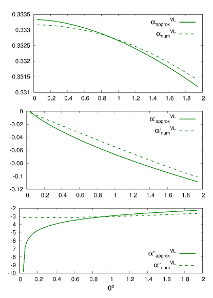
Care needs to be exercised in evaluating these expressions: each of the terms are separately infinite at Θ=0Θ0\Theta=0, and, moreover, the derivatives also act on the “star” terms, which changes the character of the integrand over the the source direction 𝐩𝐩{\bf p}. The longitudinal terms can no longer be evaluated in closed form for all ΘΘ\Theta. Ignoring the star terms yield the expressions quoted in Eq.(II). These expressions are valid everywhere for the transverse modes, but are only valid for Θ1/(fL)much-greater-thanΘ1𝑓𝐿\Theta\gg 1/(fL) for the longitudinal modes. Figure 5 compares analytic and numerical evaluations of αVL(Θ),αVL(Θ),α′′VL(Θ)superscript𝛼VLΘsuperscript𝛼VLΘsuperscript𝛼′′VLΘ\alpha^{\rm VL}(\Theta),\alpha^{\prime\rm VL}(\Theta),\alpha^{\prime\prime\rm VL}(\Theta). The numerical evaluation includes the contribution from the star terms, while the analytic expressions do not. We see that star term plays an important role in determining the small angle behavior of α′′VL(Θ)superscript𝛼′′VLΘ\alpha^{\prime\prime\rm VL}(\Theta). The same if true for α′′(Θ)superscript𝛼′′Θ\alpha^{\prime\prime}(\Theta) and σ′′(Θ)superscript𝜎′′Θ\sigma^{\prime\prime}(\Theta) all the polarization modes.

The correlation functions for the longitudinal modes are enhanced at small angles.
Refer to caption
Figure 5: Comparing the analytic expressions without the star term for αVL(Θ),αVL(Θ),α′′VL(Θ)superscript𝛼VLΘsuperscript𝛼VLΘsuperscript𝛼′′VLΘ\alpha^{\rm VL}(\Theta),\alpha^{\prime\rm VL}(\Theta),\alpha^{\prime\prime\rm VL}(\Theta) to a numerical evaluation with the star terms illustrates the differences that occur at small angles, which h are especially significant for the α′′VL(Θ)superscript𝛼′′VLΘ\alpha^{\prime\prime\rm VL}(\Theta) term. The star terms play an important role in determining the behavior of the EE(Θ)EEΘ{\rm EE}(\Theta) and BB(Θ)BBΘ{\rm BB}(\Theta) correlation functions for small angles. The plots are shown for fL=10𝑓𝐿10fL=10.

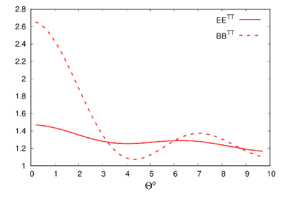
To study the small angle behavior of the correlation functions in more detail we re-write Eq.(35) in terms of α¯(Θ,𝐩)¯𝛼Θ𝐩\bar{\alpha}(\Theta,\bf p) and σ¯(Θ,𝐩)¯𝜎Θ𝐩\bar{\sigma}(\Theta,\bf p), where α(Θ)=𝑑Ω𝐩α¯(Θ,𝐩)𝛼Θdifferential-dsubscriptΩ𝐩¯𝛼Θ𝐩\alpha(\Theta)=\int d\Omega_{\bf p}\,\bar{\alpha}(\Theta,\bf p) and similarly for σ(Θ)𝜎Θ\sigma(\Theta). The correlation functions are then given by EE(Θ)=𝑑Ω𝐩ee(Θ,𝐩)EEΘdifferential-dsubscriptΩ𝐩eeΘ𝐩{\rm EE}(\Theta)=\int d\Omega_{\bf p}\,{\rm ee}(\Theta,\bf p) and similarly for BB, where the integrands ee(Θ,𝐩)eeΘ𝐩{\rm ee}(\Theta,\bf p) and bb(Θ,𝐩)bbΘ𝐩{\rm bb}(\Theta,\bf p) are finite at Θ=0Θ0\Theta=0. Using these expressions we find several interesting results: First, the EE and BB correlation functions for the transverse traceless modes are not equal at small angles since

EETT(Φs)|Θ=0=2215+𝒪(1Φs2)evaluated-atsuperscriptEETTsubscriptΦ𝑠Θ02215𝒪1superscriptsubscriptΦ𝑠2\displaystyle{\rm EE}^{\rm TT}(\Phi_{s})|_{\Theta=0}=\frac{22}{15}+\mathcal{O}\Big{(}\frac{1}{\Phi_{s}^{2}}\Big{)}
BBTT(Φs)|Θ=0=83+𝒪(1Φs2).evaluated-atsuperscriptBBTTsubscriptΦ𝑠Θ083𝒪1superscriptsubscriptΦ𝑠2\displaystyle{\rm BB}^{\rm TT}(\Phi_{s})|_{\Theta=0}=\frac{8}{3}+\mathcal{O}\Big{(}\frac{1}{\Phi_{s}^{2}}\Big{)}\,. (36)

The fact that EETT(Θ)BBTT(Θ)superscriptEETTΘsuperscriptBBTTΘ{\rm EE}^{\rm TT}(\Theta)\neq{\rm BB}^{\rm TT}(\Theta) at small angles was missed by Book and Flanagan Book and Flanagan (2011) since they neglected the star terms. A similar small-angle departure from the Hellings-Downs curve occurs due to the pulsar terms Mingarelli and Sidery (2014). Note that equality between EE and BB can not be used as a null test of general relativity at small angular separations.
Refer to caption
Figure 6: The EE and BB correlation functions for the TT mode at small angular separations. The star terms break the equality between EE and BB. The plots are shown for fL=10𝑓𝐿10fL=10.

Second, we find that the VL correlations are enhanced by a leading factor that is logarithmic in fL𝑓𝐿fL:

EEVL(Φs)|Θ=0=2ln(2Φs)3815+2γE+𝒪(1Φs)evaluated-atsuperscriptEEVLsubscriptΦ𝑠Θ02ln2subscriptΦ𝑠38152subscript𝛾𝐸𝒪1subscriptΦ𝑠\displaystyle{\rm EE}^{\rm VL}(\Phi_{s})|_{\Theta=0}=2\,\text{ln}(2\,\Phi_{s})-\frac{38}{15}+2\gamma_{E}+\mathcal{O}\Big{(}\frac{1}{\Phi_{s}}\Big{)}
BBVL(Φs)|Θ=0=2ln(2Φs)143+2γE+𝒪(1Φs).evaluated-atsuperscriptBBVLsubscriptΦ𝑠Θ02ln2subscriptΦ𝑠1432subscript𝛾𝐸𝒪1subscriptΦ𝑠\displaystyle{\rm BB}^{\rm VL}(\Phi_{s})|_{\Theta=0}=2\,\text{ln}(2\,\Phi_{s})-\frac{14}{3}+2\gamma_{E}+\mathcal{O}\Big{(}\frac{1}{\Phi_{s}}\Big{)}\,. (37)

Third, the SL modes are enhanced by a leading factor that is linear in fL𝑓𝐿fL:

EESL(Φs)|Θ=0=12[1910+3γE+π3Φs\displaystyle{\rm EE}^{\rm SL}(\Phi_{s})|_{\Theta=0}=\frac{1}{2}\Big{[}-\frac{19}{10}+3\gamma_{E}+\frac{\pi}{3}\Phi_{s}
log(2Φs)+𝒪(1Φs)],\displaystyle\hskip 93.95122pt-\text{log}(2\,\Phi_{s})+\mathcal{O}\Big{(}\frac{1}{\Phi_{s}}\Big{)}\Big{]}, (38)

where γEsubscript𝛾𝐸\gamma_{E} is the Euler-Gamma constant. The enhanced response to longitudinal gravitational waves will allow us to place far more stringent bounds on the energy density in these modes. The majority of stars in the Gaia catalog are at distances of L=0.110𝐿0.110L=0.1\rightarrow 10 kpc Astraatmadja and Bailer-Jones (2016) and the duration and cadence of the Gaia mission will allow us to probe gravitational frequencies between 3×1093superscript1093\times 10^{-9} Hz and 5×1075superscript1075\times 10^{-7} Hz Moore et al. (2017). Thus the typical values for fL𝑓𝐿fL will range between 30 and 5×1055superscript1055\times 10^{5}, and the bounds for the SL mode in particular should be orders of magnitude tighter than for the usual TT modes of GR.

V Discussion

Astrometry is a promising new approach for detecting gravitational waves Book and Flanagan (2011); Klioner (2018); Moore et al. (2017). Astrometry is particularly well suited to constraining the polarization content of gravitational waves. The expressions for the two-point correlation functions and the E and B mode correlation patterns that we have computed here provide a starting point for the analysis of data from the Gaia mission Gaia Collaboration et al. (2016). Implementing such an analysis will be challenging: our expressions for the EE and BB correlations assumed a uniform distribution of stars on the sky, and we placed all the stars at the same distance from the Earth. In reality the Gaia’s sky coverage will be non-uniform in location and distance, and techniques similar to those used in cosmic microwave background analyses will have to be used to extract the uniform correlation patterns from experiments with non-uniform sky coverage Hinshaw et al. (2003); Mignard and Klioner (2012). The vanishing of the BB correlations for scalar polarizations and the near-equality of the EE and BB polarization modes for general relativity provides a potentially powerful null test. It will be interesting to assess how the power of this test is impacted by non-uniform sky coverage and observation noise. In addition to measuring the locations of billions of stars in our galaxy, Gaia will also measure the locations of thousands of quasars. These quasars are at vastly larger distances, making the fL𝑓𝐿fL dependent enhancements for the longitudinal modes much more significant. Pairs of nearby quasars, or individual strongly lensed quasars that produce multiple images, may well provide the strongest limits to the energy density of longitudinal polarization states.

Acknowledgments

We appreciate the support of the NSF Physics Frontiers Center Award PFC-1430284.

References

  • Abbott et al. (2016a) B. P. Abbott et al. (Virgo, LIGO Scientific), Phys. Rev. Lett. 116, 061102 (2016a), eprint 1602.03837.
  • Abbott et al. (2017a) B. P. Abbott et al. (Virgo, LIGO Scientific), Phys. Rev. Lett. 119, 161101 (2017a), eprint 1710.05832.
  • Cornish et al. (2017a) N. Cornish, D. Blas, and G. Nardini, Phys. Rev. Lett. 119, 161102 (2017a), eprint 1707.06101.
  • Abbott et al. (2017b) B. P. Abbott et al. (Virgo, Fermi-GBM, INTEGRAL, LIGO Scientific), Astrophys. J. 848, L13 (2017b), eprint 1710.05834.
  • Abbott et al. (2016b) B. P. Abbott et al. (Virgo, LIGO Scientific), Phys. Rev. Lett. 116, 221101 (2016b), eprint 1602.03841.
  • Abbott et al. (2017c) B. P. Abbott et al. (Virgo, LIGO Scientific) (2017c), eprint 1709.09203.
  • Abbott et al. (2017d) B. P. Abbott et al. (Virgo, LIGO Scientific), Phys. Rev. Lett. 119, 141101 (2017d), eprint 1709.09660.
  • Abbott et al. (2018) B. P. Abbott et al. (Virgo, LIGO Scientific) (2018), eprint 1802.10194.
  • Chatziioannou et al. (2012) K. Chatziioannou, N. Yunes, and N. Cornish, Phys. Rev. D86, 022004 (2012), [Erratum: Phys. Rev.D95,no.12,129901(2017)], eprint 1204.2585.
  • Lee et al. (2008) K. J. Lee, F. A. Jenet, and R. H. Price, Astrophys. J.  685, 1304-1319 (2008).
  • da Silva Alves and Tinto (2011) M. E. da Silva Alves and M. Tinto, Phys. Rev. D83, 123529 (2011), eprint 1102.4824.
  • Chamberlin and Siemens (2012) S. J. Chamberlin and X. Siemens, Phys. Rev. D85, 082001 (2012), eprint 1111.5661.
  • Cornish et al. (2017b) N. J. Cornish, L. O’Beirne, S. R. Taylor, and N. Yunes (2017b), eprint 1712.07132.
  • Book and Flanagan (2011) L. G. Book and E. E. Flanagan, Phys. Rev. D83, 024024 (2011), eprint 1009.4192.
  • Klioner (2018) S. A. Klioner, Class. Quant. Grav. 35, 045005 (2018), eprint 1710.11474.
  • Moore et al. (2017) C. J. Moore, D. P. Mihaylov, A. Lasenby, and G. Gilmore, Phys. Rev. Lett. 119, 261102 (2017), URL https://link.aps.org/doi/10.1103/PhysRevLett.119.261102.
  • Gaia Collaboration et al. (2016) Gaia Collaboration, T. Prusti, J. H. J. de Bruijne, A. G. A. Brown, A. Vallenari, C. Babusiaux, C. A. L. Bailer-Jones, U. Bastian, M. Biermann, D. W. Evans, et al., A&A 595, A1 (2016), eprint 1609.04153.
  • Will (2014) C. M. Will, Living Reviews in Relativity 17, 4 (2014), ISSN 1433-8351, URL https://doi.org/10.12942/lrr-2014-4.
  • Yunes and Siemens (2013) N. Yunes and X. Siemens, Living Reviews in Relativity 16 (2013), URL http://www.livingreviews.org/lrr-2013-9.
  • Mihaylov et al. (2018) D. P. Mihaylov, C. J. Moore, J. R. Gair, A. Lasenby, and G. Gilmore (2018), eprint 1804.00660.
  • Mignard and Klioner (2012) F. Mignard and S. Klioner, Astron. Astrophys. 547, A59 (2012), eprint 1207.0025.
  • Mingarelli and Sidery (2014) C. M. F. Mingarelli and T. Sidery, Phys. Rev. D90, 062011 (2014), eprint 1408.6840.
  • Astraatmadja and Bailer-Jones (2016) T. L. Astraatmadja and C. A. L. Bailer-Jones, The Astrophysical Journal 833, 119 (2016), URL http://stacks.iop.org/0004-637X/833/i=1/a=119.
  • Hinshaw et al. (2003) G. Hinshaw et al. (WMAP), Astrophys. J. Suppl. 148, 135 (2003), eprint astro-ph/0302217.