Varying Random Coefficient Models

Abstract

This paper analyzes unobserved heterogeneity when observed characteristics are modeled nonlinearly. The proposed model builds on varying random coefficients (VRC) that are determined by nonlinear functions of observed regressors and additively separable unobservables. This paper proposes a novel estimator of the VRC density based on weighted sieve minimum distance. The main example of sieve bases are Hermite functions which yield a numerically stable estimation procedure. This paper shows inference results that go beyond what has been shown in ordinary RC models. We provide in each case rates of convergence and also establish pointwise limit theory of linear functionals, where a prominent example is the density of potential outcomes. In addition, a multiplier bootstrap procedure is proposed to construct uniform confidence bands. A Monte Carlo study examines finite sample properties of the estimator and shows that it performs well even when the regressors associated to RC are far from being heavy tailed. Finally, the methodology is applied to analyze heterogeneity in income elasticity of demand for housing.

Keywords: Random Coefficients, Varying Coefficients, Sieve Minimum Distance,

Hermite Functions, Rate of convergence, Bootstrap uniform confidence bands.

JEL classification: C14, C21

1 Introduction

Heterogeneity in individual behavior is a common source of variation in microeconometric applications. Thus, in recent years it became increasingly popular to explicitly model unobserved heterogeneity, for instance, by introducing random coefficients. Yet identification in random coefficient models requires functional form restrictions. This paper shows that one can be much more flexible with respect to observed characteristics which can essentially influence the shape of the density of random coefficients. Specifically we extend the ordinary random coefficient model to allow for nonlinearities in observed heterogeneity, captured by varying coefficients.

The varying random coefficient (VRC) model is given by

$$Y =B_{0}+B_{1}^{\prime}X,$$ (1.1)

where $Y$ is a scalar dependent variable and $X$ is a vector of covariates of dimension $d-1$. The VRC vector $B=(B_{0},B_{1}^{\prime})^{\prime}$ satisfies

$$B_{0}=g_{0}(W)+A_{0}\quad\text{and}\quad B_{1,l} =g_{l}(W)+A_{1,l}\quad\text{ where }1\leq l\leq d-1$$ (1.2)

for some covariates $W$ and unobservables $A=(A_{0},A_{1,1},\dots,A_{1,d-1})^{\prime}$. The varying coefficient functions $g_{0}(\cdot),\dots,g_{d-1}(\cdot)$ are unknown and capture nonlinearities in observed heterogeneity. The vectors $X$ and $W$ may have elements in common but, to ensure identification of the varying coefficient functions in general, we rule out that $X$ is a subvector of $W$. In this model, the varying random slope (VRS) given by $B_{1}$ represents observed and unobserved heterogeneity in the dependence of $Y$ on $X$. The VRC is thus more general than the ordinary random coefficient (RC) model where all varying coefficient functions vanish and hence, $B=A$. Identification of the VRC model is based on full independence of $A$ and $X$ but only conditional mean independence of $A$ and $(X,W)$. While identification of the model requires $X$ to have enough variation, our setup permits $W$ to be discrete.

This paper is concerned with inference on the density of the VRC vector $B$ holding observed characteristics $W$ fixed. This density contains all the information of the underlying heterogeneity in the model and many functionals of it are of interest, e.g., the distribution of potential outcomes. A density estimator based on weighted sieve minimum distance is proposed that builds on a conditional characteristic function equation of the model. The estimation criterion is minimized over a finite dimensional sieve space which is also convenient to impose shape restrictions on the estimator. The estimator is of closed form if no constraints are imposed on the sieve space and then coincides with a double series least squares estimator. An initial weighting step is used in the estimation criterion to stabilize the procedure. This is important, as it is well known that estimation of the joint RC density in ordinary RC models leads to an ill-posed inverse problem. One insight of this paper is that our procedure allows us to separate estimation of the VRS density from estimation of the varying random intercept $B_{0}$. In particular, we show that estimation of the VRS density does not suffer from the ill-posed estimation problem once we impose finite dimensional restrictions on the density of $B_{0}$.

For the sieve minimum distance estimator, inference results are established that go beyond what has been obtained in ordinary RC models. The rate of convergence of the estimator is derived, which coincides with the usual ill-posed rate of convergence when estimating the joint VRC density and corresponds to the usual well-posed, nonparametric rate when only the density of VRS is of interest and semiparametric restrictions on the random intercept are imposed. Many important objects of interest, such as the distribution of the potential outcome, are functionals of the density of $B$. For a plug-in estimator of such linear functionals we establish pointwise asymptotic normality. This paper also provides a bootstrap procedure to construct uniform confidence bands of the estimator. The inference results in this paper make explicit how the marginal distribution of $X$ affects the asymptotic behavior of the estimator.

Identification of the model requires a large support condition of $X$ in general. Yet under mild assumptions, identification can be also achieved under bounded support via extrapolation. This motivates the use of global basis functions for the sieve minimum distance estimator, such as the Hermite functions. When the sieve space is spanned by Hermite functions, we see that the estimator considerably simplifies as these basis functions form eigenfunctions of the Fourier transform. The estimator performs well in finite samples even when covariates $X$ are far from being heavy tailed. This is demonstrated in Monte Carlo simulations that also clarify how the variance of $X$ affects the mean integrated squared error of the estimator in finite samples.

The estimation procedure is also applied to analyze heterogeneity in income elasticity of housing demand using German survey data. In our specification, estimated observed housing characteristics exhibit a nonlinear shape. The estimated density of heterogeneous income elasticity is unimodal with mode close to zero and positively skewed. Uniform confidence bands allow to make significant statements about the shape of the estimated density. The empirical application demonstrates that our proposed methodology can be useful to analyze complex heterogeneity using cross sectional data.

Nonparametric identification and estimation of ordinary RC models is considered by Beran and Hall [1992], Beran et al. [1996], and Hoderlein et al. [2010]. For testing of qualitative features of the ordinary RC models see Dunker et al. [2019]. Lewbel and Pendakur [2017] generalize these models to allow for nonlinear index functions and in the next section we will provide a more detailed comparison of it to the VRC model. The ordinary RC models can be extended to conditional random coefficient models that assume model equation (1.1) together with the condition that $X$ is independent of $B$ conditional on $W$. This model is more flexible than $(\ref{mod:gen}$–$\ref{mod:gen:rc})$, but requires that the conditional density of $X$ given $W$ satisfies a large support condition for all realizations of $W$. Beyond this more restrictive support restriction, estimation in conditional RC models also suffers from the curse of dimensionality of $W$. This is why functional form restrictions are typically employed rather than considering the more general conditional RC models, see for instance, [Lewbel and Pendakur, 2017, p. 1120]. Recently, correlated random coefficient models were studied in the literature which allow for full dependence of random coefficients and covariates $X$. In this setting, instruments are available that drive the covariates $X$ but not the random coefficients in (1.1). These types of models are analyzed by Masten [2018] and Hoderlein et al. [2017]. While such a model is clearly more general than the VRC model, identification of the CRC models can be challenging with more restrictive exclusion assumptions and large support conditions on the instruments.

The methodology of sieve estimation became increasingly popular in recent years. For sieve estimation of conditional moment restrictions models see Newey and Powell [2003] and Ai and Chen [2003]. The VRC model does not fall into this category. For sieve estimation of ordinary RC models with discrete outcome see Fox et al. [2011] and Fox et al. [2016]. In binary choice models, Gautier and Le Pennec [2018] proposed an estimator based on needlet thresholding. In the context of specification testing, a sieve approach was used by Breunig and Hoderlein [2018]. In the literature on varying coefficients, series estimators were analyzed by Xia and Li [1999], Fan et al. [2003], Xue and Wang [2012], or Ma and Song [2015].

The remainder of the paper is organized as follows. Section 2 provides the setup, motivating examples, and sufficient conditions for nonparametric identification. In Section 3, the estimation procedure based on sieve minimum distance is introduced and its asymptotic properties are established. Section 4 is concerned with the finite sample properties of the estimator analyzed via Monte Carlo simulation and an empirical illustration. Section 5 concludes. All proofs can be found in the appendix.

2 The Model and Identification

This section consists of two subsections. Subsection 2.1 recalls the varying random coefficients (VRC) model, outlines its key properties, and provides motivating examples for it. Subsection 2.2 provides an identification result of the joint density of the VRC vector $B$.

2.1 The Varying Random Coefficient Model

Consider again equations $(\ref{mod:gen}$–$\ref{mod:gen:rc})$, the VRC model is given by

$$Y =B_{0}+B_{1}^{\prime}X,$$ (1.1)

$$B_{0} =g_{0}(W)+A_{0}\quad\text{and}\quad B_{1,l}=g_{l}(W)+A_{1,l}\quad\text{ where }1\leq l\leq d-1.$$ (1.2)

As stated above $X$ and $W$ may have elements in common. Yet without further functional form restrictions on the varying coefficient functions $g_{0},\dots,g_{d-1}$ we need to rule out that $X$ has only elements that are contained in $W$ (see also Assumption 1 and the discussion thereafter). The covariates $X$ are assumed to be independent of $A$ and the vector of covariates $(X^{\prime},W^{\prime})^{\prime}$ is restricted to be mean independent of $A$, i.e., $\operatorname{\mathbb{E}}[A|X,W]=0$ (see Assumption 1 below). All the results in this paper will hold if there were no varying coefficients, i.e., model $(\ref{mod:gen}$–$\ref{mod:gen:rc})$ is the ordinary RC model. While identification of the model requires $X$ to have enough variation, our setup permits $W$ to be discrete.

Under conditional mean independence of $A$ and $(X,W)$, model $(\ref{mod:gen}$–$\ref{mod:gen:rc})$ implies the varying coefficient model

$$\operatorname{\mathbb{E}}[Y|X,W]=g_{0}(W)+\sum_{l=1}^{d-1}g_{l}(W)X_{l}=:g(S),$$ (2.1)

using the notation $S=(X^{\prime},W^{\prime})^{\prime}$. In the conditional mean restriction (2.1), the varying coefficient functions $g_{l}$ are identified through a rank condition, see also below. For an overview article of varying coefficient models see Park et al. [2015]. We emphasize that the varying coefficients specification in (2.1) also derives from the additive separability of the random coefficients $A$ in equation (1.2). Without imposing such an additively separable structure, our model is in general not identified, see [Masten, 2018, Corollary 2]. On the other hand, under further assumptions, Lewbel and Pendakur [2017] establish identification when equation (1.1) is replaced by $Y=B_{0}+\sum_{l=1}^{d-1}G_{l}(B_{1,l}X_{l})$ for unknown functions $G_{l}$ and $A$ is independent of $(X,W)$ (it is thus non-nested to our VRC model). While the sieve minimum distance approach in this paper allows for estimation of additional nonlinear index functions, we do not consider this extension.

Identification of the varying coefficient functions $g_{0},\dots,g_{d-1}$ in the VRC model $(\ref{mod:gen}$–$\ref{mod:gen:rc})$ can be obtained in the following two scenarios: First, under a full rank condition on $\operatorname{\mathbb{E}}[XX^{\prime}|W=w]$ or, second, if $g_{1}\equiv\dots\equiv g_{d-1}\equiv 0$. In the first case, the VRC model has the interpretation similar to a conditional random coefficient model but, instead of leaving the distribution of $X$ and $W$ unrestricted, it imposes more structure on it. Also similarly to conditional random coefficient models, the role of $W$ is to ensure that independence between $A$ and $X$ is more plausible. The variables $W$ can also serve as control function residuals, which then allows $X$ to be endogenous, i.e., $A$ is unconditionally correlated with $X$. In the second case, only $g_{0}$ differs from the zero function and thus the VRC model has the interpretation of a nonlinear model in $X$, when $X=W$, but with random coefficients only on the linear term.

This paper is concerned with estimation of the VRC density holding the observed characteristics fixed at some potential realization $w$, i.e., the density $f_{B}(\cdot,w)$ of

$$B^{w}=\mathbf{g}(w)+A$$

where $\mathbf{g}(\cdot)=(g_{0}(\cdot),\dots,g_{d-1}(\cdot))^{\prime}$ denotes the vector of varying coefficient functions. In the case where $X$ and $W$ have no common elements, $B^{w}$ captures heterogeneous marginal effects. If $X$ and $W$ have joint elements then, to obtain marginal effects, replace $\mathbf{g}(w)$ with the vector of partial derivatives of $\mathbf{g}(w)$ w.r.t. $x$. The results in this paper are still valid in this case but it is not made explicit in order to keep the notation simple. By holding observed characteristics $W$ fixed, the density $f_{B}(\cdot,w)$ contains all information on unobserved heterogeneity. Many objects of interest, such as the density of potential outcomes of $Y$, are linear functionals of $f_{B}(\cdot,w)$.

Economic theory and empirical findings suggest nonlinearities in many applications of interest. For instance, through a nonparametric analysis of Engel curves to analyze nonlinearities in total expenditure, Banks et al. [1997] suggest quadratic terms in the logarithm of total expenditure. While a random coefficient version of their nonlinear model is not identified one might still account for unobserved heterogeneity by allowing only the coefficient for the linear term to vary among individuals. The following two examples provide a relation of VRC to measurement error models and show that ignoring nonlinearities in the varying coefficients may have severe consequences in a standard Monte Carlo exercise setting.

Example 2.1 (Measurement Error Models).

Consider a regression model with interaction term and measurement error in one covariate:

$$Y=\beta_{0}+\beta_{1}X_{1}+\beta_{2}X_{1}X_{2}^{*}+\beta_{3}X_{2}^{*}+U,$$ (2.2)

where the variable $X_{2}^{*}$ is observed only with measurement error, i.e., $X_{2}=X_{2}^{*}+V$. The deterministic parameters $\beta_{l}$, $1\leq l\leq 3$, are unknown, and $(U,V)$ are unobservables with zero mean. Assume that an additional variable $W$, the instrumental variable, is available which satisfies $X_{2}^{*}=m(W)+\widetilde{A}$ where $W$ is conditional mean independent of $\widetilde{A}$ and $V$ (see, for instance, Hausman et al. [1991], Schennach [2007], or Ben-Moshe et al. [2017]). The conditional mean restriction identifies the parameters $\beta_{0},\dots,\beta_{3}$ since the function $m(W)=\operatorname{\mathbb{E}}[X_{2}|W]$ is identified. Using the instrumental variables approach we can rewrite the model (2.2) as

$$Y=\underbrace{\beta_{0}+\beta_{3}m(W)}_{g_{0}(W)}+\underbrace{\beta_{3}\widetilde{A}+U}_{A_{0}}+\big{(}\underbrace{\beta_{1}+\beta_{2}m(W)}_{g_{1}(W)}+\underbrace{\beta_{2}\widetilde{A}}_{A_{1}}\big{)}X_{1}$$

and thus, is a special case of the VRC model $(\ref{mod:gen}$–$\ref{mod:gen:rc})$.

Example 2.2 (Monte Carlo Simulation under misspecification).

This finite sample example shows that falsely assuming linearity of varying coefficient functions may lead to severe biases that go beyond typical approximation errors. Here, draws of regressors $(X,W)$ are generated from the bivariate standard normal distribution. Let $Y=A_{0}+B_{1}X$ where $B_{1}=2W^{2}+A_{1}$ and random coefficients $(A_{0},A_{1})$ are generated independently of $(X,W)$ as follows: $A_{1}$ is drawn from a mixture of normal distributions, i.e., $\mathcal{N}\left(-1.5,2\right)$ and $\mathcal{N}\left(1.5,1\right)$ with weights $0.5$, and independently from $A_{0}\sim\mathcal{N}(0,1)$.

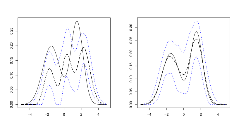
Figure 1: Solid lines: true density $f_{B_{1}}(\cdot,w)$ with $w=0$. Dotted lines: median and pointwise $95\%$ confidence intervals. Left: Using OLS estimator of $g_{1}$. Right: Using B-splines estimator of $g_{1}$. Sample Size: $n=1000$. Monte Carlo iterations: $1000$.

We implement our estimator using Hermite functions, as described in the Monte Carlo section, but estimate the function $g_{1}(w)=2w^{2}$ once via ordinary least squares (OLS) and once via quadratic B-splines with three interior knots. Figure 1 shows on the left the resulting estimator when $g_{1}$ is estimated via OLS and on the right when $g_{1}$ is estimated via B-splines. From Figure 1 we see that ignoring the nonlinearity in $g_{1}$ can imply additional nonlinearities in the resulting estimator of the density of $B_{1}$.

2.2 Identification

This section provides assumptions under which the density $f_{B}(\cdot,w)$ of $B^{w}$ is identified for any value $w$ in the support of $W$. We now impose restrictions on the observed and unobserved variables of our model.

Assumption 1.

(i) $X$ is independent of $A$. (ii) $(X^{\prime},W^{\prime})$ is mean independent of $A$, i.e., $\operatorname{\mathbb{E}}[A|X,W]=0$. (iii) $\mathbf{g}(\cdot)=(g_{0}(\cdot),\dots,g_{d-1}(\cdot))^{\prime}$ is identified through the conditional moment equation (2.1).

An independence assumption similar to Assumption 1 is common in the literature on RC models with cross-sectional data (see, for instance, Beran [1993], Beran et al. [1996], Hoderlein et al. [2010]). It should be also emphasized that the independence assumption can often be justified in our model if the information in $W$ about heterogeneity is rich enough and in this sense is milder than in the ordinary RC model where $\mathbf{g}\equiv 0$. Clearly, if $W$ contains only elements in $X$ and $\operatorname{\mathbb{E}}[A]=0$ then Assumption 1 (ii) is implied by (i).

Assumption 1 (iii) is automatically satisfied if $g_{l}\equiv 0$ for all $1\leq l\leq d-1$. Otherwise, Assumption 1 (iii) is satisfied if for all $w$ in the support of $W$, the smallest eigenvalue of $\operatorname{\mathbb{E}}[XX^{\prime}|W=w]$ is bounded away from zero. This rank condition is commonly imposed in the varying coefficient literature. In particular, it rules out that the vector of regressors $X$ has only values that are also contained in the vector $W$. It is also possible to relax the rank condition by imposing functional form restrictions on $g$, see Fan et al. [2003]. Throughout the paper, the conditional characteristic function of $Y-g(S)$ given $X$ is denoted by $h(x,t;g)=\operatorname{\mathbb{E}}\big{[}\exp\big{(}it(Y-g(S))\big{)}\big{|}X=x\big{]}$.

Assumption 2.

(i) $X$ has full support $\mathbb{R}^{d-1}$. (ii) $\int_{\mathbb{R}^{d-1}}\int_{\mathbb{R}}|t|^{d-1}|h(x,t;g)|dt\,dx<\infty$.

While large support conditions are often required in econometrics to ensure identification, Assumption 2 (i) can be relaxed. If the distribution of $A$ has finite absolute moments and is uniquely determined by its moments, then identification with bounded support of $X$ can be achieved by extrapolation, see Masten [2018] and Hoderlein et al. [2017]. Assumption 2 (ii) imposes a mild regularity assumption on the conditional characteristic function $h$.

The next result establishes identification of the VRC density. We make use of identification of the varying coefficients through the conditional mean restriction (2.1). Consequently, by employing the relation $f_{B}(b,w)=f_{A}(b-\mathbf{g}(w))$ the following result is due to Fourier inversion.

Lemma 2.1.

Let Assumptions 1–2 be satisfied. Then, for all $w$ in the support of $W$, the density of $B^{w}$ satisfies

$$f_{B}(b,w)=\frac{1}{(2\pi)^{d}}\int_{\mathbb{R}^{d-1}}\int_{\mathbb{R}}|t|^{d-1}\exp\big{(}-it(1,x^{\prime})(b-\mathbf{g}(w))\big{)}h(x,t;g)dt\,dx.$$

Lemma 2.1 shows that the density $f_{B}(\cdot,w)$ can be written as a transform of varying coefficient functions. Besides the shift of the conditional characteristic function $\operatorname{\mathbb{E}}[\exp(itY)|X=x]$ to $h(x,t;g)$ there is also a location shift by $\mathbf{g}(w)$. This corresponds to shifts in frequency and time domain for the Fourier transform.

3 Estimation and Inference

This section presents an estimator of the VRC density based on sieve minimum distance and establishes its asymptotic properties. Subsection 3.1 introduces the weighted sieve minimum distance estimator and motivates the use of Hermite functions as sieve basis. In Subsection 3.2, the rate of convergence of the estimator of $f_{B}$ is derived. Subsection 3.3 establishes the pointwise asymptotic distribution of linear functionals of $f_{B}$, where the density of potential outcome is one particular example of interest. Subsection 3.4 presents a Bootstrap procedure to construct uniform confidence bands.

3.1 The Sieve Minimum Distance Estimator

Estimation builds on the conditional characteristic function equation induced by the model $(\ref{mod:gen}$–$\ref{mod:gen:rc})$. We denote the Fourier transform by $(\mathcal{F}\phi)(u):=\int_{\mathbb{R}^{d}}\exp(iu^{\prime}z)\phi(z)dz$ for any absolutely integrable function $\phi$. Recall the notation of the conditional characteristic function $h(x,t;g)=\operatorname{\mathbb{E}}[\exp(it(Y-g(S)))|X=x]$. Independence of $X$ and $A$, as imposed in Assumption 1, immediately implies

$$\operatorname{\mathbb{E}}\big{[}\exp\big{(}it(A_{0}+A_{1}^{\prime}X)\big{)}\big{|}X=x\big{]}=\int_{\mathbb{R}^{d}}\exp\big{(}it(1,x^{\prime})a\big{)}f_{A}(a)da=\big{(}\mathcal{F}f_{A}\big{)}(t,tx)$$

and hence the relation

$$\big{(}\mathcal{F}f_{A}\big{)}(t,tx)=h(x,t;g)$$ (3.1)

for all $t\in\mathbb{R}$ and $x\in\mathbb{R}^{d-1}$. Moreover, relation (3.1) leads to

$$\int_{\mathbb{R}^{d-1}}\int_{\mathbb{R}}\Big{|}\big{(}\mathcal{F}f_{A}\big{)}(t,tx)-h(x,t;g)\Big{|}^{2}d\nu(t)dx=0,$$ (3.2)

for some measure $\nu$. Using this $L^{2}$ criterion we construct a sieve minimum distance estimator of $f_{A}$ and use a plug-in approach to estimate the VRC density $f_{B}$. Below, we show that the choice of the log-normal distribution as weighting measure $\nu$ is well suited for our estimation problem.

The proposed sieve minimum distance estimator of the VRC density $f_{B}(\cdot,w)$ is based on the relation $f_{B}(b,w)=f_{A}(b-\mathbf{g}(w))$ for any $w$ in the support of $W$: Consider the plug-in estimator

$$\widehat{f}_{B}(b,w)=\widehat{f}_{A}(b-\mathbf{\widehat{g}}(w))$$ (3.3)

where $\widehat{f}_{A}$ is a sieve minimum distance estimator of $f_{A}$ given by

$$\widehat{f}_{A}\in\operatorname*{arg\,min}_{f\in\mathcal{A}_{K}}\Big{\{}\int_{\mathbb{R}^{d-1}}\int_{\mathbb{R}}\big{|}(\mathcal{F}f)(t,tx)-\widehat{h}(x,t;\widehat{g})\big{|}^{2}d\nu(t)dx\Big{\}}$$

and $\mathcal{A}_{K}$ is a sieve space of dimension $K=K(n)<\infty$ with basis functions $\{q_{k}\}_{k\geq 1}$. The sieve dimension $K=K(n)$ grows slowly with sample size $n$. Sieve estimation is also convenient to impose additional constraints on the unknown functions. These constraints, such as positivity, can be directly imposed on the sieve space $\mathcal{A}_{K}$. When the constraints are not binding, we may consider $\mathcal{A}_{K}$ without constraints, which then coincides with the linear sieve space $\mathcal{A}_{K}=\big{\{}\phi(\cdot)=\beta^{\prime}q^{K}(\cdot):\,\beta\in\mathbb{R}^{K}\big{\}}$ where $q^{K}(\cdot)=\big{(}q_{1}(\cdot),\dots,q_{K}(\cdot)\big{)}^{\prime}$.

The unknown conditional characteristic function $h$ is replaced by the plug-in series least squares estimator

$$\widehat{h}(x,t;\widehat{g})=p^{K}(x)^{\prime}\widehat{P}^{-1}\frac{1}{n}\sum_{j=1}^{n}\exp\big{(}it(Y_{j}-\widehat{g}(S_{j}))\big{)}p^{K}(X_{j}),$$ (3.4)

where $p^{K}(\cdot)=\big{(}p_{1}(\cdot),\dots,p_{K}(\cdot)\big{)}^{\prime}$ is a vector of basis functions and we use the notation $\widehat{P}=n^{-1}\sum_{j=1}^{n}p^{K}(X_{j})p^{K}(X_{j})^{\prime}$. Thus, the same sieve dimension $K$ (as for $\mathcal{A}_{K}$) is used to approximate the conditional characteristic function $h$. The estimator $\widehat{g}$ of the regression function $g$ is based on the conditional mean restriction (2.1). We do not impose an explicit form of this estimator but rather impose a rate condition on the estimator $\widehat{g}$ to obtain our asymptotic results. In particular, $\widehat{g}$ can account for generated regressors when $W$ are control function residuals. Below, Example 3.2 provides an illustration of estimating $g$ via series least squares. Although estimation of the density $f_{B}$ involves two preliminary steps (estimation of $h$ and $g$) it should be emphasized that the estimation procedure is equivalent to a one-step sieve minimum distance estimator, which, additionally involves the conditional characteristic equation $h(X,t;g)=\operatorname{\mathbb{E}}\big{[}\exp\big{(}it(Y-g(S))\big{)}\big{|}X\big{]}$ and the conditional moment equation (2.1).

When no constraints are imposed, the sieve minimum distance estimator (3.3) is of closed form. In this case, $\widehat{f}_{B}$ coincides with the double series least squares estimator

$$\widehat{f}_{B}(b,w)=q^{K}(b-\widehat{\mathbf{g}}(w))^{\prime}Q^{-1}\int_{\mathbb{R}^{d-1}}\int_{\mathbb{R}}\big{(}\mathcal{F}q^{K}\big{)}(-t,-tx)\,\widehat{h}(x,t;\widehat{g})d\nu(t)\,dx$$

where

$$Q=\int_{\mathbb{R}^{d-1}} \int_{\mathbb{R}}\big{(}\mathcal{F}q^{K}\big{)}(-t,-tx)\big{(}\mathcal{F}q^{K}\big{)}(t,tx)^{\prime}d\nu(t)dx$$ (3.5)

is assumed to be nonsingular (at least for $K$ sufficiently large). Nonsingularity of $Q$ is satisfied by Hermite functions (under mild conditions) which, as the following example illustrates, are a convenient choice of bases for the sieve space $\mathcal{A}_{K}$.

Example 3.1 (Hermite Functions).

Consider a linear sieve space $\mathcal{A}_{K}$ spanned by Hermite functions (which are orthonormalized Hermite polynomials) given for $k=0,1,2,\dots$ by

$$q_{k+1}(t)=\frac{(-1)^{k}}{\sqrt{2^{k}k!\sqrt{\pi}}}\exp(t^{2}/2)\frac{d^{k}}{dt^{k}}\exp(-t^{2}).$$

These functions form an orthonormal basis in $L^{2}(\mathbb{R})={\left\{\phi:\int_{\mathbb{R}}\phi^{2}(t)dt<\infty\right\}}$ and are convenient in our framework: Hermite functions are eigenfunctions of the Fourier transform satisfying $(\mathcal{F}q_{k+1})(t)/\sqrt{2\pi}=i^{k}q_{k+1}(t)=:\widetilde{q}_{k+1}(t)$. Thus, the double series least squares estimator of $f_{B}$ given in (3.3) simplifies to

$$\widehat{f}_{B}(\cdot,w)=q^{K}(\cdot-\widehat{\mathbf{g}}(w))^{\prime}Q^{-1}\int_{\mathbb{R}^{d-1}}\int_{\mathbb{R}}\widetilde{q}^{K}(-t,-tx)\widehat{h}(x,t;\widehat{g})d\nu(t)\,dx,$$ (3.6)

where $Q=(2\pi)^{d/2}\int_{\mathbb{R}^{d-1}}\int_{\mathbb{R}}\widetilde{q}^{K}(-t,-tx)\widetilde{q}^{K}(t,tx)^{\prime}d\nu(t)dx$. The implementation of this estimator is straightforward. In the finite sample analysis, we also estimate the conditional characteristic function $h$ using Hermite functions.

We now consider the case of tensor product basis functions. We make use of the notation $\text{I}_{K_{1}}$ for the $K_{1}$-dimensional identity matrix and $\otimes$ for the Kronecker product.

Lemma 3.1.

Let $\mathcal{A}_{K}$ be a linear sieve space spanned by tensor product Hermite functions $q^{K}(t,u)=q^{K_{0}}(t)\otimes q^{K_{1}}(u)$ where $K=K_{0}K_{1}$. Then, the matrix $Q$ given in (3.5) simplifies to

$$Q=Q_{0}\otimes\text{I}_{K_{1}}\quad\text{ where }\quad Q_{0}=(2\pi)^{d/2}\int_{\mathbb{R}}|t|^{1-d}\widetilde{q}^{K_{0}}(-t)\widetilde{q}^{K_{0}}(t)^{\prime}d\nu(t).$$

Lemma 3.1 shows that given tensor product Hermite functions in a linear sieve space only the dimension parameter $K_{0}$ used to approximate the random intercept induces potentially small eigenvalues of $Q$ and hence, slow accuracy of estimators. Thus, if we are willing to restrict the complexity of sieve estimation in terms of $K_{0}$, for instance, by imposing a fixed dimension $K_{0}$, then the rate of convergence does not suffer from an ill-posed inverse problem. This semiparametric specification provides a numerically stable estimation procedure as we see in our Monte Carlo simulation section.

Remark 3.1 (VRS Density Estimation).

The proposed methodology implies closed form estimators of densities of subvectors of the VRC vector. Consider the setup of Lemma 3.1 with a linear sieve space and $q^{K}(t,u)=q^{K_{0}}(t)\otimes q^{K_{1}}(u)$ are Hermite functions. The double series least squares estimator (3.6) yields the estimator of the VRS density $f_{B_{1}}(\cdot,w)$ given by

$$\widehat{f}_{B_{1}}(\cdot,w)=q^{K_{1}}(\cdot-\widehat{\mathbf{g}}_{1}(w))^{\prime}\int_{\mathbb{R}^{d-1}}\int_{\mathbb{R}}b_{K_{0}}(t)\widetilde{q}^{K_{1}}(-tx)\widehat{h}(x,t;\widehat{g})d\nu(t)\,dx$$ (3.7)

where

$$b_{K_{0}}(t):=\int_{\mathbb{R}}q^{K_{0}}(a)^{\prime}da\,Q_{0}^{-1}\widetilde{q}^{K_{0}}(-t).$$

Here, $K_{1}$ coincides with the dimension of basis functions used for the estimator $\widehat{h}$. Note that we impose restrictions on the weighting measure $\nu$ below such that $\int_{\mathbb{R}}|t|^{1-d}d\nu(t)$ is bounded above and away from zero and hence, $Q_{0}$ is well defined.

Example 3.2 (Series estimation of the varying coefficients).

We provide an explicit estimator of the mean regression function $g(s)=\operatorname{\mathbb{E}}[Y|S=s]$. Series estimation of $g$ is convenient, in particular, as an additive structure of $g$ can be easily imposed. To do so, consider the basis functions $p_{k}$, $k\geq 1$, and introduce the vector $p_{d}^{K}(s)=\big{(}p^{K}(w)^{\prime},x_{1}p^{K}(w)^{\prime},\dots,x_{d-1}p^{K}(w)^{\prime}\big{)}^{\prime}\in\mathbb{R}^{dK}$. The series least squares estimator of $g$ is given by

$$\widehat{g}(s)=p_{d}^{K}(s)^{\prime}\widehat{P}_{d}^{-1}\sum_{j=1}^{n}Y_{j}p_{d}^{K}(S_{j}),$$

where $\widehat{P}_{d}=n^{-1}\sum_{j=1}^{n}p^{K}_{d}(S_{j})p^{K}_{d}(S_{j})^{\prime}$. For instance, when using B-Splines as basis functions, for asymptotic properties of such estimators see Xia and Li [1999], Fan et al. [2003], Xue and Wang [2012], or Ma and Song [2015].

Notation.

Introduce the norms $\|\phi\|_{\nu}=\big{(}\int_{\mathbb{R}}\int_{\mathbb{R}^{d-1}}|\phi(x,t)|^{2}dxd\nu(t)\big{)}^{1/2}$ and $\|\phi\|_{\mathbb{R}^{d}}=\big{(}\int_{\mathbb{R}^{d}}|\phi(u)|^{2}du\big{)}^{1/2}$ with associated Hilbert spaces $L^{2}_{\nu}={\left\{\phi:\|\phi\|_{\nu}<\infty\right\}}$ and $L^{2}(\mathbb{R}^{d})={\left\{\phi:\|\phi\|_{\mathbb{R}^{d}}<\infty\right\}}$. Moreover, $\|\cdot\|$ and $\|\cdot\|_{\infty}$ denote the $\ell_{2}$–norm and the supremum norm. For a matrix $A$, the operator norm is denoted by $\|A\|$. For a random vector $V$ the corresponding calligraphic capital letter $\mathcal{V}$ denotes its support. Let $\Pi_{K}:L^{2}(\mathbb{R}^{d})\to\mathcal{A}_{K}$ denote the least squares projection onto $\mathcal{A}_{K}$, i.e., $\Pi_{K}f=\operatorname*{arg\,min}_{\phi\in\mathcal{A}_{K}}\|\phi-f\|_{\mathbb{R}^{d}}$ for all $f\in L^{2}(\mathbb{R}^{d})$. Further, define the function $\gamma:\mathbb{R}\to\mathbb{R}^{K}$ given by $\gamma(t)=P^{-1}\operatorname{\mathbb{E}}[\exp\big{(}it(Y-g(S))\big{)}p^{K}(X)]$ where we recall $P=\operatorname{\mathbb{E}}[p^{K}(X)p^{K}(X)^{\prime}]$. We use the notation $a_{n}\sim b_{n}$ for $cb_{n}\leq a_{n}\leq Cb_{n}$ given two constant $c,C>0$ and all $n\geq 1$.

3.2 Rate of Convergence

This subsection provides rates of convergence of the proposed estimators. In particular, we see that only the rate of the VRC density hinges on the minimal eigenvalues of $Q$. On the other hand, it is shown below that the rate of convergence of the estimator of the varying random slope $B_{1}$ is not affected by the choice of $\nu$.

We introduce an assumption required for our asymptotic results. Below, $\lambda_{\max}(M)$ denotes the maximal eigenvalue of a matrix $M$. Throughout the paper, $(\tau_{k})_{k\geq 1}$ and $(\lambda_{k})_{k\geq 1}$ denote nonincreasing sequences.

Assumption 3.

(i) A random sample ${\left\{(Y_{i},X_{i},W_{i})\right\}}_{i=1}^{n}$ of $(Y,X,W)$ is observed. (ii) The measure $\nu$ satisfies $0<\int_{\mathbb{R}}|t|^{1-d}d\nu(t)<\infty$, $\int_{\mathbb{R}}t^{2}d\nu(t)<\infty$ and $\|h(\cdot,\cdot;g)\|_{\nu}<\infty$. (iii) $\lambda_{\max}\big{(}\int_{\mathbb{R}^{d-1}}p^{K}(x)p^{K}(x)^{\prime}dx\big{)}=O(1)$ and $\lambda_{\max}\big{(}\int_{\mathbb{R}^{d}}q^{K}(a)q^{K}(a)^{\prime}da\big{)}=O(1)$. (iv) $\lambda_{\max}(\lambda_{K}P^{-1})=O(1)$ and $\sup_{x\in\mathbb{R}^{d-1}}\|p^{K}(x)\|^{2}=O(K)$ satisfying $K\log(n)=o(n\lambda_{K})$. (v) $\lambda_{\max}(\tau_{K}Q^{-1})=O(1)$ and $\|\mathcal{F}(\Pi_{K}f_{A}-f_{A})\|_{\nu}^{2}=O(\tau_{K}\|\Pi_{K}f_{A}-f_{A}\|_{\mathbb{R}^{d}}^{2})$.

Assumption 3 (ii) imposes a mild restriction on the weighting measure $\nu$ and is satisfied, for instance, if $\nu$ is the log-normal distribution. The maximal eigenvalue restriction imposed in Assumption 3 (iii) is automatically satisfied if $\{p_{k}\}_{k\geq 1}$ and $\{q_{k}\}_{k\geq 1}$ form orthonormal bases in $L^{2}(\mathbb{R}^{d-1})$ and $L^{2}(\mathbb{R}^{d})$, respectively. Assumption 3 (iv) allows the minimal eigenvalues of $P$ to tend to zero, see also Chen and Christensen [2015], who consider a similar restriction on the growth of basis functions. This condition holds for Hermite functions, which are uniformly bounded, but also for polynomial splines, Fourier series and wavelet bases, see also Belloni et al. [2015] for further discussion and extensions of Newey [1997]. It is well known, that the smallest eigenvalue of $P$ is uniformly bounded away from zero if ${\left\{p_{l}\right\}}_{l\geq 1}$ forms an orthonormal basis and $f_{X}$ is uniformly bounded away from zero on the support of $X$. Thus, Assumption 3 (iv) is particularly suited in our case where a large support assumption of $X$ is required for identification. Here, $\lambda_{K}$ has the interpretation of a truncation parameter in estimation problems to ensure that the denominator is bounded away from zero, see Breunig and Hoderlein [2018]. Assumption 3 (v) imposes a rate restriction on the minimal eigenvalue of the matrix $Q$ relative to $(\tau_{k})_{k\geq 1}$. Assumption 3 (v) further specifies a link of the sieve approximation error on the RC density $f_{A}$ between the “strong” norm $\|\cdot\|_{\mathbb{R}^{d}}$ and the “weak” norm $\|\cdot\|_{\nu}$. Note that Assumption 3 (v) is only required for estimating the VRC density but not for estimating the VRS density. Such stability conditions are commonly imposed in the literature on nonparametric instrumental variable estimation, see, for instance, Blundell et al. [2007] or Chen and Pouzo [2012], but rely on mapping properties of an unknown conditional expectation operator. In addition, in VRC models it is possible to provide primitive conditions, as we see below.

Proposition 3.2.

Let $\widetilde{\nu}(t):=|t|^{1-d}(d\nu/d\mu)(t)$ where $\mu$ denotes the Lebesgue measure and assume that $\{q_{k}\}_{k\geq 1}$ is an orthonormal basis in $L^{2}(\mathbb{R}^{d})$.

• Suppose that, for some constant $0<c<1$, for all $n\geq 1$ and any non-zero vector $a\in\mathbb{R}^{K}$ the inequality

  $$\int_{\mathbb{R}}\big{|}a^{\prime}(\mathcal{F}q^{K})(t)\big{|}^{2}\mathop{\mathbbm{1}}\nolimits\nolimits{\left\{\widetilde{\nu}(t)<\tau_{K}\right\}}\mu(dt)\leq c\int_{\mathbb{R}}\big{|}a^{\prime}(\mathcal{F}q^{K})(t)\big{|}^{2}\mu(dt)$$ (3.8)

  holds. Then, the smallest eigenvalue of $\tau_{K}^{-1}Q$ is bounded away from zero and bounded above.

• If

  $$\sum_{l>K}\int_{\mathbb{R}}\big{|}(\mathcal{F}q_{l})(t)\big{|}^{2}\,\widetilde{\nu}(t)d\mu(t)=O(\tau_{K})$$ (3.9)

  then $\|\mathcal{F}(\Pi_{K}f_{A}-f_{A})\|_{\nu}^{2}=O\big{(}\tau_{K}\|\Pi_{K}f_{A}-f_{A}\|_{\mathbb{R}^{d}}^{2}\big{)}$.

In the case of Hermite functions, condition (3.8) requires $\nu$ to be sufficiently heavy tailed while condition (3.9) requires $\int_{\mathbb{R}}\big{|}(\mathcal{F}q_{l})(t)\big{|}^{2}\,\widetilde{\nu}(t)d\mu(t)$ to be sufficiently small for all $l>K$. Both conditions impose restrictions on the weighting measure $\nu$ and the basis functions $\{q_{k}\}_{k\geq 1}$ but do not on the unknown density $f_{A}$ itself. The following example discusses the log-normal distribution as a weighting measure and provides primitive conditions for inequality (3.8).

Example 3.3 (Log-normal weighting).

The weighting measure $\nu$ is given by the distribution $\textsl{Lognormal}(0,\sigma^{2})$ for some $\sigma>0$. Thus, the function $\widetilde{\nu}$ as introduced in Proposition 3.2 coincides with $\widetilde{\nu}(t)=\exp\big{(}-(\log t)^{2}/(2\sigma^{2})\big{)}/(\sqrt{2\pi}\sigma\,t^{d})$ for all $t\geq 0$. In this case, $\widetilde{\nu}(t)<\tau_{K}$ if and only if $\exp\big{(}-(\log t)^{2}/(2\sigma^{2})\big{)}<\tau_{K}\sqrt{2\pi}\sigma t^{d}$ which holds for all $t\geq 0$ satisfying

$$(\log t)^{2}/(2\sigma^{2})+d(\log t)+\log\big{(}\sqrt{\pi}\sigma\tau_{K}\big{)}>0.$$

Note that Hermite functions have most of its support close to zero when $K$ is chosen moderately and hence, inequality (3.8) is always satisfied for $\tau_{K}$ sufficiently small. The decay of the eigenvalues of $Q$ can be directly computed via numerical approximation of the integral.

We impose regularity conditions on the unknown functions of interest. To do so, we introduce the space of square integrable functions $L_{S}^{2}=\big{\{}\phi:\|\phi\|_{S}:=\sqrt{\operatorname{\mathbb{E}}\phi^{2}(S)}<\infty\big{\}}$. Further, we define the class of functions $\mathcal{G}:=\mathcal{G}(n):=\{\phi=\beta^{\prime}p_{d}^{K}:\|\phi-g\|_{\infty}\leq\sqrt{K/n}\}$. The covering number $N(\mathcal{G},\|\cdot\|_{S},\epsilon)$ is the minimal number of $L_{S}^{2}$–balls of radius $\epsilon$ needed to cover $\mathcal{G}$.

Assumption 4.

(i) $\|\Pi_{K}f_{A}-f_{A}\|_{\mathbb{R}^{d}}=O(K^{-\zeta/d})$ and $\|\gamma^{\prime}p^{K}-h\|_{\nu}=O(K^{-\rho/(d-1)})$. (ii) $f_{A}$ is continuously differentiable with square integrable Jacobian matrix $Df_{A}$. (iii) $\|\widehat{g}-g\|_{\infty}^{2}=O_{p}(K/n)$ and $\|\widehat{\mathbf{g}}(w)-\mathbf{g}(w)\|^{2}=O_{p}\big{(}K/(n\tau_{K}\lambda_{K})\big{)}$ for all $w\in\mathcal{W}$. (iv) There exists $C_{n}>0$ with $C_{n}\sqrt{K/n}=O(1)$ such that $\int_{0}^{1}\sqrt{1+\log N(\mathcal{G},\|\cdot\|_{S},\epsilon)}d\epsilon\leq C_{n}<\infty$.

Assumption 4 (i) captures regularity conditions on the density $f_{A}$ and the conditional characteristic function $h$ via sieve approximation errors. Example 3.4 characterizes the sieve approximation condition when using Hermite basis functions relative to the smoothness of the unknown function of interest. For further discussion and other examples of sieve bases, see Chen [2007]. Assumption 4 (ii) imposes a mild smoothness condition on the density $f_{A}$. Assumption 4 (iii) imposes rate restrictions on the varying coefficients estimator. Assumption 4 (iv) is a regularity condition on the function class $\mathcal{G}$ and was also imposed in the literature, for instance, in [Chen and Pouzo, 2012, Lemma C.3 (i)].

Example 3.4 (Hermite functions (cont’d)).

Consider again the case where the linear sieve space $\mathcal{A}_{K}$ is spanned by Hermite functions. If $f_{A}$ has $2\zeta$ derivatives such that $\int f^{(\iota)}(x)dx<\infty$ for all $\iota\leq 2\zeta$ then the sieve approximation condition $\|\Pi_{K}f_{A}-f_{A}\|_{\mathbb{R}^{d}}=O(K^{-\zeta/d})$ in Assumption 4 (i) is automatically satisfied due to Lemma 2 of Coppejans and Gallant [2002]. See also Bongioanni and Torrea [2009] where a Sobolev space for Hermite functions is constructed (and also in the case of Laguerre polynomials). On the other hand, if $A$ has compact support and $f_{A}$ belongs to a Sobolev ellipsoid of smoothness $\zeta$ then the sieve approximation error $O(K^{-\zeta/d})$ is obtained for B-splines, wavelets, or trigonometric basis functions, see Chen [2007].

Consider first estimation of the joint density of the VRC vector $B$ holding observed characteristics fixed. The following theorem provides the rate of convergence in $L^{2}(\mathbb{R}^{d})$–norm of the estimator $\widehat{f}_{B}(\cdot,w)$ given in (3.3) for some fixed $w\in\mathcal{W}$.

Theorem 3.1.

Let Assumptions 1–4 be satisfied. Then for any $w\in\mathcal{W}$:

$$\int_{\mathbb{R}^{d}}\big{|}\widehat{f}_{B}(b,w)-f_{B}(b,w)\big{|}^{2}db=O_{p}\left((\tau_{K}\lambda_{K})^{-1}\Big{(}n^{-1}K+K^{-2\rho/(d-1)}\Big{)}+K^{-2\zeta/d}\right).$$

We see from the previous result that the parameters $\tau_{K}$ and $\lambda_{K}$, which capture the minimal eigenvalues of $Q$ and $P$, respectively, slow down the rate of convergence. As the weighting measure $\nu$ influences the eigenvalues of $Q$ it does also affect the rate of convergence of the joint density of the varying random coefficient $B$. Note that the optimal choice of the dimension parameter $K$ is lower than for usual nonparametric estimation problems and relative to the value of $\tau_{K}$ and $\lambda_{K}$.

We now provide the rate of convergence in $L^{2}(\mathbb{R}^{d})$–norm of $\widehat{f}_{B}$ when the dimension parameter $K$ is chosen such that the variance part $(n\tau_{K}\lambda_{K})^{-1}K$ and the squared bias part $K^{-2\zeta/d}$ are of the same order. For ease of exposition we assume that $\lambda_{K}$ is uniformly bounded away from zero, which requires a sufficiently large support of regressors $X$. We further consider the case that $n^{-1}K$ dominates the squared bias part of estimating $h$ which is $K^{-2\rho/(d-1)}$. The next result immediately follows from Theorem 3.1 and hence, its proof is omitted.

Corollary 3.1.

Let Assumptions 1–4 be satisfied. Further if $\lambda_{K}$ is uniformly bounded away from zero, $\tau_{K}\sim K^{-2\alpha/d}$, $K\sim n^{d/{(2\zeta+2\alpha+d)}}$ and if

$$\frac{\alpha+\zeta}{d}\leq\frac{\rho}{(d-1)}$$ (3.10)

holds, then for any $w\in\mathcal{W}$:

$$\int_{\mathbb{R}^{d}}\big{|}\widehat{f}_{B}(b,w)-f_{B}(b,w)\big{|}^{2}db=O_{p}\Big{(}n^{-2\zeta/(2\zeta+2\alpha+d)}\Big{)}.$$

As we see from the previous result, the usual rate of convergence for ill-posed inverse problems is obtained if $K$ levels variance and squared bias, see also Hoderlein et al. [2010] in the case of kernel estimation in ordinary RC models. Yet in contrast to Hoderlein et al. [2010] (see their Section 4.3), no heavy-tailedness of covariates $X$ is required for our convergence results. In particular, Hohmann and Holzmann [2016] showed under Gaussian white noise that the rate of convergence can be much slower, even severely ill-posed, under lighter tails of $X$. Also note that the condition (3.10) ensures that $n^{-1}K$ dominates the squared bias of estimating $h$ and is only a mild restriction. Indeed, if, for instance, $d=2$ then the usual rate of convergence is obtained if $2\rho\geq\zeta+\alpha$.

Below, we establish a rate of convergence for estimating the density of the varying random slope $B_{1}$ holding observed characteristics $W$ fixed. The next results show that for estimating the VRS vector $B_{1}$ when we restrict the sieve dimension, to approximate the random intercept, to be bounded. In this case the rate of convergence does not depend on the eigenvalue behavior of the matrix $Q$.

Theorem 3.2.

Let Assumptions 1, 2, 3 (i)–(iv), and 4 be satisfied where $q^{K}(t,u)=q^{K_{0}}(t)\otimes q^{K_{1}}(u)$ are tensor product Hermite functions with $K_{0}=O(1)$. Then the closed form estimator $\widehat{f}_{B_{1}}(\cdot,w)$ given in (3.7) satisfies for any $w\in\mathcal{W}$:

$$\int_{\mathbb{R}^{d-1}}\big{|}\widehat{f}_{B_{1}}(b_{1},w)-f_{B_{1}}(b_{1},w)\big{|}^{2}db_{1}=O_{p}\Big{(}\lambda_{K_{1}}^{-1}\Big{(}n^{-1}K_{1}+K_{1}^{-2\rho/(d-1)}\Big{)}+K_{1}^{-2\zeta/(d-1)}\Big{)}.$$

Note that the condition $K_{0}=O(1)$ together with Assumption 4 (i), that is, $\|\Pi_{K}f_{A}-f_{A}\|_{\mathbb{R}^{d}}=O(K^{-\zeta/d})$, imposes a semiparametric restriction on the RC density $f_{A}$. We emphasize that the parametric restriction concerns only the random intercept $A_{0}$ but not the random slope $A_{1}$. Also the rate of convergence derived in the previous result depends on the dimension parameter $K_{1}$ only. This is due to the definition of our estimator where the dimension of basis functions used to estimate the conditional characteristic function $h$ coincides with the dimension parameter $K_{1}$, see also Remark 3.1. Similarly to Theorem 3.2, convergence rates of subvector VRS densities can be derived.

The following result provides the rate of convergence when the dimension parameter $K_{1}$ such that the variance part $(n\lambda_{K_{1}})^{-1}K$ and the squared bias $K_{1}^{-2\zeta/d}$ are of the same order and $n^{-1}K_{1}$ dominates the squared bias of estimating $h$. Again we consider the case where $\lambda_{K_{1}}$ is uniformly bounded away from zero. The next result immediately follows from Theorem 3.2 and hence, its proof is omitted.

Corollary 3.2.

Let the conditions of Theorem 3.2 be satisfied. Further, if $\lambda_{K_{1}}$ is uniformly bounded away from zero, $K_{1}\sim n^{(d-1)/{(2\zeta+d-1)}}$ and $\zeta\leq\rho$ holds, then the closed form estimator $\widehat{f}_{B_{1}}(\cdot,w)$ given in (3.7) satisfies for any $w\in\mathcal{W}$:

$$\int_{\mathbb{R}^{d-1}}\big{|}\widehat{f}_{B_{1}}(b,w)-f_{B_{1}}(b,w)\big{|}^{2}db=O_{p}\Big{(}n^{-2\zeta/(2\zeta+d-1)}\Big{)}.$$

As we see from the previous result, the rate of convergence coincides with the usual optimal rate in nonparametric density of dimension $d-1$. We see that the rate for estimating the density of the varying random slope $B_{1}$ is not affected by the ill-posedness under the condition $K_{0}=O(1)$.

3.3 Pointwise Limit Theory for Linear Functionals

This subsection is about inference of linear functionals $\ell(\cdot):L^{2}(\mathbb{R}^{d})\to\mathbb{R}$ of the density $f_{B}(\cdot,w)$ for some realization $w$ of $W$. Examples of linear functionals are, but are not limited to, the point-evaluation functional or (weighted) averages of $f_{B}(\cdot,w)$. The linear functional $\ell(f_{B}(\cdot,w))$ is estimated below using the plug-in sieve estimate estimator $\ell(\widehat{f}_{B}(\cdot,w))$. This subsection provides a limit theory for this plug-in estimator.

As mentioned in the introduction, an important example of a linear functional of $f_{B}$ is the density of the potential outcome $Y^{s}=\mathbf{g}(w)^{\prime}x+A^{\prime}x$, where $s=(x^{\prime},w^{\prime})^{\prime}$. Indeed, the density of $Y^{s}$ can be written as

$$f_{Y}(y,s)=\int_{\mathbb{R}^{d-1}}f_{B}\big{(}(y-x^{\prime}b_{1},b_{1}),w\big{)}\,db_{1}.$$

Also the weighted averages of potential outcomes $\int_{\mathbb{R}}\omega(y)f_{Y}\big{(}y,s\big{)}dy$ for some function $\omega$ is a linear functional of $f_{B}(\cdot,w)$. In particular, we obtain the distribution of the potential outcomes which is relevant also in the context of quantile treatment effects.

The asymptotic distribution result below requires the following additional notation and assumptions. We introduce the sieve variance

$$\textsl{v}_{K}(w) =\ell\big{(}q^{K}(\cdot-\mathbf{g}(w))\big{)}^{\prime}Q^{-1/2}\,\Sigma\,Q^{-1/2}\ell\big{(}q^{K}(\cdot-\mathbf{g}(w))\big{)}$$ (3.11)

where

$$\Sigma=\int_{\mathbb{R}}\int_{\mathbb{R}}R(s)P^{-1}\operatorname{\mathbb{E}}\Big{[}p^{K}(X)\rho(s)\rho(-t)p^{K}(X)^{\prime}\Big{]}P^{-1}R(-t)^{\prime}d\nu(s)d\nu(t),$$

using the notation $\rho(t)=\exp(it(Y-g(S)))-h(X,t;g)$ and the matrix valued function $R(t)=Q^{-1/2}\int_{\mathbb{R}^{d-1}}(\mathcal{F}q^{K})(t,tx)p^{K}(x)^{\prime}dx$. We replace the sieve variance $\textsl{v}_{K}$ by the estimator

$$\widehat{\textsl{v}}_{K}(w) =\ell\big{(}q^{K}(\cdot-\widehat{\mathbf{g}}(w))\big{)}^{\prime}Q^{-1/2}\,\widehat{\Sigma}\,Q^{-1/2}\ell\big{(}q^{K}(\cdot-\widehat{\mathbf{g}}(w))\big{)},$$ (3.12)

where the matrix $\Sigma$ is replaced by

$$\widehat{\Sigma}=\int_{\mathbb{R}}\int_{\mathbb{R}}R(s)\widehat{P}^{-1}\frac{1}{n}\sum_{j=1}^{n}p^{K}(X_{j})\widehat{\rho}_{j}(s)\widehat{\rho}_{j}(-t)p^{K}(X_{j})^{\prime}\widehat{P}^{-1}R(-t)^{\prime}d\nu(s)d\nu(t),$$

with $\widehat{\rho}_{j}(t)=\exp(it(Y_{j}-\widehat{g}(S_{j})))-\widehat{h}(X_{j},t;\widehat{g})$. In order to derive the asymptotic distribution of our estimator we require addition assumptions. Below, we denote the inverse Fourier transform by $(\mathcal{F}^{-1}\phi)(u)=(2\pi)^{-d}\int_{\mathbb{R}^{d}}\exp(-itu)\phi(t)dt$.

Assumption 5.

(i) The minimal eigenvalue of $\lambda_{K}^{-1}\Sigma$ is uniformly bounded away from zero. (ii) It holds $C_{n}^{2}K^{2}=o(n\lambda_{K})$. (iii) For all $w\in\mathcal{W}$: $\sqrt{n}\ell\big{(}\Pi_{K}f_{A}(\cdot-\mathbf{g}(w))-f_{A}(\cdot-\mathbf{g}(w))\big{)}=o\big{(}\sqrt{\textsl{v}_{K}(w)}\big{)}$, $\sqrt{n}\ell\big{(}[\mathcal{F}^{-1}(\gamma^{\prime}p^{K}-h)](\cdot-\mathbf{g}(w))\big{)}=o\big{(}\sqrt{\textsl{v}_{K}(w)}\big{)}$, and $\sqrt{n}\big{\|}\widehat{\mathbf{g}}(w)-\mathbf{g}(w)\big{\|}=o_{p}\big{(}\sqrt{\textsl{v}_{K}(w)}\big{)}$. (iv) The sieve space $\mathcal{A}_{K}$ is linear: $\mathcal{A}_{K}=\big{\{}\phi(\cdot)=\beta^{\prime}q^{K}(\cdot):\,\beta\in\mathbb{R}^{K}\big{\}}$ and $q_{l}$, $l\geq 1$, are continuously differentiable. (v) It holds $\int_{\mathbb{R}}\|R(t)\|^{2}d\nu(t)=O(1)$.

Assumption 5 (i) implies a lower bound on the sieve variance which we require to achieve asymptotic distribution results of the estimator. This condition implies that the sieve variance attains the lower bound $\textsl{v}_{K}(w)\geq C_{\Sigma}\,\|\ell\big{(}q^{K}(\cdot-\mathbf{g}(w))\big{)}^{\prime}Q^{-1/2}\|^{2}/\lambda_{K}$ for some constant $C_{\Sigma}>0$. For instance, when $\ell(\cdot)$ is the point evaluation functional and $Q$ is a diagonal matrix with polynomial decay of order $-2\alpha/d$ we obtain $\textsl{v}_{K}(w)\geq C_{\Sigma}\,K^{(2\alpha+d)/d}$ provided that $\lambda_{K}$ is bounded from below and $\|q^{K}(a-\mathbf{g}(w))\|^{2}\geq K$ which holds at most points $a\in\mathcal{A}$ (see Belloni et al. [2015]). Consequently the lower bound of the sieve variance corresponds to the mildly ill-posed case in [Chen and Pouzo, 2015, p. 1053]. Assumption 5 (ii) imposes a stronger rate requirement on $K$ than the one required for consistency. Assumption 5 (iii) specifies a pointwise sieve approximation error and has the interpretation of an undersmoothing condition, which is required to ensure that the approximation bias is asymptotically negligible. Assumption 5 (iv) restricts the sieve space to be linear and, in particular, that constraints on density estimation, such as positivity, are not binding. If such constraints are binding asymptotically then such shape restriction can lead to non-normal distributions. Assumption 5 (v) is automatically satisfied if the basis under consideration is given by Hermite functions.

Assumption 6.

It holds $\zeta_{n}=o(1)$ where $\zeta_{n}=\sqrt{K\log(n)/(n\tau_{K}\lambda_{K})}+K^{1/2-\rho/(d-1)}$ and $\|\gamma^{\prime}p^{K}-h\|_{\nu}=O(K^{-\rho/(d-1)})$.

Assumption 6 strengthens the rate conditions imposed in Assumption 5 and is required for consistent estimation of the sieve variance $\textsl{v}_{K}(w)$. The next result establishes the asymptotic distribution of the estimator $\ell(\widehat{f}_{B}(\cdot,w))$.

Theorem 3.3.

Let Assumptions 1–3, 4 (ii)–(iv), and 5 be satisfied. Then, for any $w\in\mathcal{W}$:

$$\sqrt{n/\textsl{v}_{K}(w)}\,\Big{(}\ell\big{(}\widehat{f}_{B}(\cdot,w)\big{)}-\ell\big{(}f_{B}(\cdot,w)\big{)}\Big{)}\stackrel{{\scriptstyle d}}{{\rightarrow}}\mathcal{N}(0,1).$$

If, in addition Assumption 6 holds, then

$$\sqrt{n/\widehat{\textsl{v}}_{K}(w)}\,\Big{(}\ell\big{(}\widehat{f}_{B}(\cdot,w)\big{)}-\ell\big{(}f_{B}(\cdot,w)\big{)}\Big{)}\stackrel{{\scriptstyle d}}{{\rightarrow}}\mathcal{N}(0,1).$$

A direct implication of the previous results concerns inference on functionals of the VRS density $f_{B_{1}}(\cdot,w)$. The next result is based on plug-in series estimator (3.7) using tensor product Hermite functions. In this case, the sieve variance simplifies to

$$\textsl{v}_{K_{1}}(w) =\ell\big{(}q^{K_{1}}(\cdot-\mathbf{g}(w))\big{)}^{\prime}\Sigma_{1}\ell\big{(}q^{K_{1}}(\cdot-\mathbf{g}(w))\big{)}$$

where the matrix $\Sigma_{1}$ is coincides with $\Sigma$ except that $K$ replaced by $K_{1}$ and $R(t)$ replaced by $\int_{\mathbb{R}^{d-1}}b_{K_{0}}(t)\widetilde{q}^{K_{1}}(tx)p^{K_{1}}(x)^{\prime}dx$, where the function $b_{K_{0}}$ is given in Remark 3.1. Now if $K_{0}=O(1)$ a lower bound for the sieve variance is $\textsl{v}_{K_{1}}(w)\geq C_{\Sigma_{1}}\,\|\ell\big{(}q^{K_{1}}(\cdot-\mathbf{g}(w))\big{)}\|^{2}/\lambda_{K_{1}}$ for some constant $C_{\Sigma_{1}}>0$. When $\lambda_{K_{1}}$ is uniformly bounded away from zero this corresponds to the usual lower bound in well posed estimation problems, see Newey [1997] or Belloni et al. [2015]. An estimator $\widehat{\textsl{v}}_{K_{1}}(w)$ of the sieve variance $\textsl{v}_{K_{1}}(w)$ is obtained by replacing the covariance matrix $\Sigma_{1}$ by $\widehat{\Sigma}_{1}$ which is analog to the definition of $\widehat{\Sigma}$. The next result is an immediate consequence of Theorem 3.3 and hence its proof is omitted.

Corollary 3.3.

Let Assumptions 1, 2, 3 (i)–(iv), 4 (ii)–(iv), 5, and 6 be satisfied where $q^{K}(t,u)=q^{K_{0}}(t)\otimes q^{K_{1}}(u)$ are tensor product Hermite functions with $K_{0}=O(1)$. Then, for any $w\in\mathcal{W}$:

$$\sqrt{n/\widehat{\textsl{v}}_{K_{1}}(w)}\,\Big{(}\ell\big{(}\widehat{f}_{B_{1}}(\cdot,w)\big{)}-\ell\big{(}f_{B_{1}}(\cdot,w)\big{)}\Big{)}\stackrel{{\scriptstyle d}}{{\rightarrow}}\mathcal{N}(0,1).$$

3.4 Bootstrap Uniform Confidence Bands

This subsection provides a bootstrap procedure to construct uniform confidence bands for $f_{B}(\cdot,w)$ and establishes asymptotic validity of it. The multiplier bootstrap procedure is as follows. Let $(\varepsilon_{1},\ldots,\varepsilon_{n})$ be a bootstrap sequence of i.i.d. random variables drawn independently of the data $\{(Y_{1},X_{1},W_{1}),\ldots,(Y_{n},X_{n},W_{n})\}$, with $\operatorname{\mathbb{E}}[\varepsilon_{j}]=0$, $\operatorname{\mathbb{E}}[\varepsilon_{j}^{2}]=1$, $\operatorname{\mathbb{E}}[|\varepsilon_{j}|^{3}]<\infty$ for all $1\leq j\leq n$. Common choices of distributions for $\varepsilon_{j}$ include the standard Normal, Rademacher, and the two-point distribution of Mammen [1993]. Further, $\mathbb{P}^{*}$ denotes the probability distribution of the bootstrap innovations $(\varepsilon_{1},\ldots,\varepsilon_{n})$ conditional on the data. For any $w\in\mathcal{W}$, we introduce the bootstrap process

$$\mathbb{Z}^{*}(b,w)=\frac{q^{K}(b-\widehat{\mathbf{g}}(w))^{\prime}Q^{-1/2}}{\sqrt{\widehat{\textsl{v}}_{K}(b,w)}}\left(\frac{1}{\sqrt{n}}\sum_{j=1}^{n}\int_{\mathbb{R}}R(t)\widehat{\rho}_{j}(t)d\nu(t)\widehat{P}^{-1}p^{K}(X_{j})\,\varepsilon_{j}\right).$$

Here, we use the notation $\textsl{v}_{K}(b,w)$ and $\widehat{\textsl{v}}_{K}(b,w)$ for the sieve variance and its estimator given in (3.11) and (3.12) in case of point-evaluation functionals. Let $\mathcal{C}$ be a closed subset of $\mathbb{R}^{d}$. Let $\Delta$ be the standard deviation semimetric on $\mathcal{C}$ of the Gaussian Process $\mathbb{Z}(b,w)=q^{K}(b-\mathbf{g}(w))^{\prime}Q^{-1/2}\mathcal{Z}/\sqrt{\textsl{v}_{K}(b,w)}$ with $\mathcal{Z}\sim\mathcal{N}(0,\Sigma)$ defined as $\Delta_{w}(b_{1},b_{2})=(\operatorname{\mathbb{E}}[(\mathbb{Z}(b_{1},w)-\mathbb{Z}(b_{2},w))^{2}])^{1/2}$, see e.g. [van der Vaart and Wellner, 2000, Appendix A.2]. To do so, we introduce the notation $N(\mathcal{C},\Delta,\epsilon)$ for the $\epsilon$-entropy of $\mathcal{C}$ with respect to norm $\Delta$.

Assumption 7.

(i) $\mathcal{C}$ is compact and $(\mathcal{C},\Delta)$ is separable for each $n\geq 1$. (ii) There exists a sequence of finite positive integers $c_{n}$ such that $1+\int_{0}^{\infty}\sqrt{\log N(\mathcal{C},\Delta_{w},\epsilon)}d\epsilon=O(c_{n})$. (iii) There exists a sequence of positive integers $r_{n}$ with $r_{n}=o(1)$ such that $K^{5/2}\lambda_{K}^{-2}=o(r_{n}^{3}\sqrt{n})$, $r_{n}c_{n}=O(1)$, and

$$\lambda_{K}^{-1}K\sqrt{\frac{\log(n)}{n}}+\sqrt{\zeta_{n}}\Big{(}c_{n}+K^{(-\rho)/(d-1)}+\sup_{b\in\mathcal{C}}\sqrt{\frac{n}{\textsl{v}_{K}(b,w)}}|\Pi_{K}f_{B}(b,w)-f_{B}(b,w)|\Big{)}=o(r_{n}).$$

(iv) It holds $\sup_{b\in\mathcal{C}}\left(\|q^{K}\big{(}b-\mathbf{g}(w)\big{)}^{\prime}Q^{-1/2}\|^{2}/\textsl{v}_{K}(b,w)\right)=O(1)$.

Assumption 7 is similar to [Chen and Christensen, 2018, Assumption 6] who establish asymptotic validity of uniform confidence bands in nonparametric instrumental variable estimation. Assumption 7 (ii) is a mild regularity assumption, see also [Chen and Christensen, 2018, Remark 4.2] for sufficient conditions. Assumption 7 (iii) strengthens the rate conditions imposed on the dimension parameter $K$ and imposes a uniform sieve approximation error.

The next theorem establishes the validity of the bootstrap for constructing uniform confidence bands for the VRC density $f_{B}(\cdot,w)$. The proof of this result is based on strong approximation of a series process by a Gaussian process, and uses an anti-concentration inequality for the supremum of the approximating Gaussian process obtained in Chernozhukov et al. [2014]. For sieve minimum distance estimation in nonparametric instrumental variable estimation this is also exploited by Chen and Christensen [2018].

Theorem 3.4.

Let the assumptions of Theorem 3.3 and Assumption 7 hold. Then for all $w\in\mathcal{W}$:

$$\sup_{s\in\mathbb{R}}\left|\mathbb{P}\left(\sup_{b\in\mathcal{C}}\left|\sqrt{\frac{n}{\widehat{\textsl{v}}_{K}(b,w)}}\Big{(}\widehat{f}_{B}(b,w)-f_{B}(b,w)\Big{)}\right|\leq s\right)-\mathbb{P}^{*}\left(\sup_{b\in\mathcal{C}}\left|\mathbb{Z}^{*}(b,w)\right|\leq s\right)\right|=o_{p}(1).$$

Theorem 3.4 establishes consistency of the sieve score bootstrap procedure for estimating the critical values of the uniform sieve t-statistic process for the VRC model. The result also contributes to the literature on ordinary RC models, as up to now, only asymptotic validity of pointwise confidence intervals is established and complements the results of Dunker et al. [2019] who proposed tests for qualitative features of the ordinary RC’s density.

4 Simulation Studies and an Empirical Illustration

This section provides a finite sample analysis of the proposed estimator. Subsection 4.1 presents the finite sample performance of the proposed estimator in Monte Carlo simulations. Subsection 4.2 applies the procedure to analyze heterogeneity in income elasticity of the willingness to pay for rent in an empirical illustration.

4.1 Simulation Studies

This subsection presents the finite-sample performance of the estimator of the varying random slope in a Monte Carlo simulation study. The experiments use a sample size of $1000$ and $1000$ Monte Carlo replications in each setting. In each experiment, i.i.d. draws of regressors $(X,W)$ are generated from

$$\begin{pmatrix}X\\ W\end{pmatrix}\sim\mathcal{N}\left(\begin{pmatrix}0\\ 0\end{pmatrix},\begin{pmatrix}\sigma^{2}&0\\ 0&1\end{pmatrix}\right)$$

where the variance $\sigma^{2}$ is varied in the experiments. Realizations of $A$ are generated independently of $(X,W)$ as follows: The random slope parameter $A_{1}$ is drawn either by a mixture of normal distributions, i.e., $\mathcal{N}\left(-1.5,1\right)$ and $\mathcal{N}\left(1.5,0.5\right)$ with weights $0.5$, or by the Gamma distribution $\Gamma(3,1)$. In each case, the random intercept is generated independently of the random slope by $A_{0}\sim\mathcal{N}(0,1)$. Realizations of the dependent variable $Y$ are obtained by

$$Y=A_{0}+XB_{1},$$ (4.1)

with varying random coefficients

$$B_{1}=g_{1}(W)+A_{1}$$ (4.2)

where in the experiments either $g_{1}(w)=\sin(w)$ or $g_{1}(w)=\exp(|w|)-1$.

In this simulation study, a linear sieve space with Hermite functions is used and no additional constraints are imposed. Consequently, the resulting estimator of the density of $B_{1}$ is of closed form as given in (3.7). Numerical integration is used to compute the integrals in equation (3.7) based on the Adaptive Gauss-Kronrod quadrature (using the pracma package in R). We keep the dimension for the random intercept fixed with $K_{0}=1$. The conditional characteristic function $h$ is estimated via series least squares as in equation (3.4) where the basis functions coincide with the Hermite functions of dimension $K_{1}$. For the estimation of the varying coefficient function $g_{1}$ we use quadratic B-spline bases with interior knots placed evenly. More precisely, we use two interior knots when using the function $g_{1}(w)=\sin(w)$ and four knots in the case of $g_{1}(w)=\exp(|w|)-1$.

Varying Coefficient	St. Dev. of $X$	$\text{MISE}(\widehat{f}_{B_{1}})$ for sieve dim.
$g_{1}(w)$	$\sigma$	$K_{1}=4$	$K_{1}=5$	$K_{1}=6$
$\sin(w)$	1/2	$\mathbf{0.0373}$	0.0642	0.3094
	$\sqrt{1/2}$	0.0184	$\mathbf{0.0167}$	0.0318
	1	0.0140	$\mathbf{0.0075}$	0.0092
	2	0.0129	0.0069	$\mathbf{0.0056}$
$\exp(|w|)-1$	1/2	$\mathbf{0.0267}$	0.0672	0.3110
	$\sqrt{1/2}$	$\mathbf{0.0156}$	0.0189	0.0336
	1	0.0126	$\mathbf{0.0088}$	0.0106
	2	0.0125	0.0091	$\mathbf{0.0070}$

Table 1: Monte Carlo Results for the $\text{MISE}(\widehat{f}_{B_{1}})$ for varying values of $\sigma$ and different functions of $g_{1}$. Bold letters show values of $\text{MISE}(\widehat{f}_{B_{1}})$ minimized w.r.t. $K_{1}$.

As weighting measure $\nu$, we choose the log-normal distribution as motivated in Example 3.3, more precisely, $\nu$ is given by $\textsl{Lognormal}(0,\sigma_{\nu}^{2})$ where $\sigma_{\nu}=1/4$.

For the implementation of the estimator it is required to choose the dimension parameter $K_{1}$, given that we have fixed the dimension $K_{0}=1$. In the Monte Carlo experiments we choose these parameters to minimize the mean integrated squared error. Table 1 reports the mean integrated squared error of the estimator $\widehat{f}_{B_{1}}(\cdot,w)$ of $f_{B_{1}}(\cdot,w)$ when $w=0$ which is given by

$$\text{MISE}(\widehat{f}_{B_{1}})=\operatorname{\mathbb{E}}\int_{-5}^{5}\big{|}\widehat{f}_{B_{1}}(b,0)-f_{B_{1}}(b,0)\big{|}^{2}db$$

where the expectation is over the mean of all simulations.

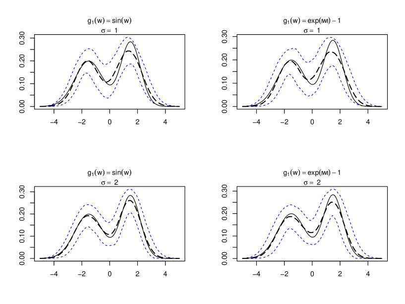
Figure 2: The first column shows the median of the estimators $\widehat{f}_{B_{1}}(\cdot,w)$, with their pointwise 95% confidence intervals when $g_{1}(w)=\sin(w)$. The second column is equivalent but uses $g_{1}(w)=\exp(|w|)-1$. The solid lines depict the true density $f_{B_{1}}(\cdot|w)$ where $w=0$.

Table 1 depicts values of $\text{MISE}(\widehat{f}_{B_{1}})$ for different values of $\sigma^{2}$ and different functions $g_{1}$. In each case, the $\text{MISE}(\widehat{f}_{B_{1}})$ is provided for different sieve dimensions $K_{1}$, where the minimized value (w.r.t. the sieve dimension $K_{1}$) is shown in bold letters. From Table 1 we see, not surprisingly, that the $\text{MISE}(\widehat{f}_{B_{1}})$ decreases as the variance of $X$ becomes larger. In particular, the optimal choice of the dimension parameter $K_{1}$ increases as the variance $\sigma^{2}$ becomes larger. This is in line with the rate of convergence as derived in Theorem 3.2, see also the discussion thereafter. The MISE when $g_{1}(w)=\exp(|w|)-1$ is larger as in the other case which is due to irregularity of the function $g_{1}$ at zero.

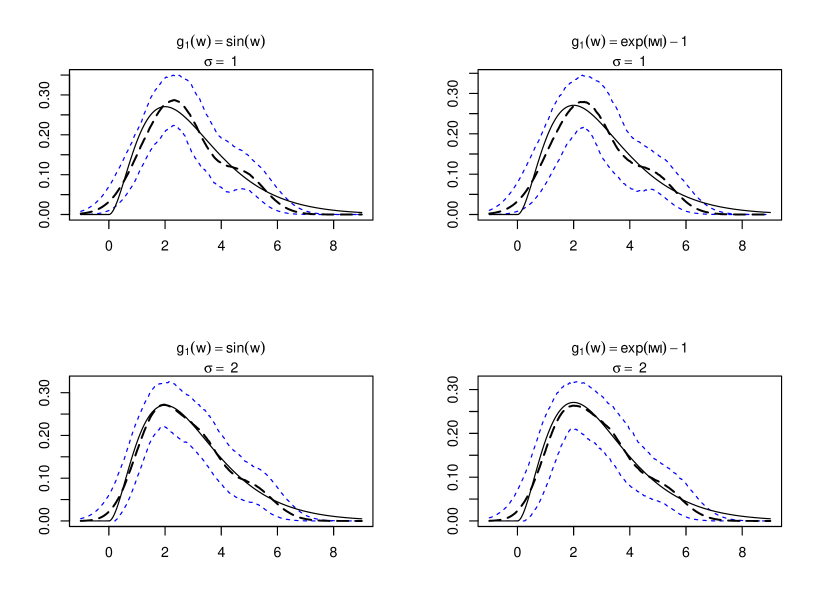
Figure 3: As in Figure 2 but where the true density, depicted as solid line, is the density of $\Gamma(3,1)$.

Figure 2 shows the estimation results when the true distribution of $B_{1}$ is given by an equally weighted mixture of $\mathcal{N}\left(-1.5,2\right)$ and $\mathcal{N}\left(1.5,1\right)$. The solid line depicts the true density $f_{B_{1}}(\cdot,w)$ with $w=0$, the thick dashed line depicts the median of the estimators, and the thin dashed lines show the $95\%$ percent pointwise confidence intervals. The number of Hermite basis functions $K_{1}$ is chosen to minimize the $\text{MISE}(\widehat{f}_{B_{1}})$ as shown in Table 1, i.e., $K_{1}=5$ when $\sigma^{2}=1$ and $K_{1}=6$ when $\sigma^{2}=2$. We see that as the variance $\sigma^{2}$ increases (lower panel of the figure) the median of the estimators is closer to the true density. Although there is no positivity constraint imposed, the closed form median of the estimator together with their $95\%$ confidence intervals are non-negative between $-5$ and $5$. As the variance of $X$ increases the pointwise confidence intervals become more narrow, which is in line with the pointwise asymptotic theory. This indicates the difficulty of estimating random coefficients in the case where $X$ has light tails. Nevertheless, we see that the estimator performs well even if $X$ has a small variance and is far from heavy tailed. Figure 2 also shows that the procedure is robust even against irregularities of the varying coefficient function, i.e., when $g_{1}$ coincides with $g_{1}(w)=\exp(|w|)-1$.

Figure 3 depicts the estimator of $f_{B_{1}}$ in the case when $A_{1}$ is generated by the Gamma distribution $\Gamma(3,1)$. For the implementation of the estimator we use the same choice of tuning parameters as described above in the normal mixture case. Again we find the $95\%$ confidence interval and the median are more accurate when the variance of $X$ is increased from $1$ to $2$ and $g_{1}$ coincides with the sine function. In all cases, we see that the true density function lies outside of the confidence intervals for $b_{1}\in[7,9]$. This bias is due to a larger variance of $A_{1}$, i.e., $\mathop{{\mathbb{V}}ar}\nolimits(A_{1})=3$, which implies that higher order Hermite functions are required to fully accurately capture the finite sample support of $A_{1}$.

We finally present estimation results when not only the random slope (again we consider $A_{1}\sim\Gamma(3,1)$) but also the random intercept is not normally distributed but $A_{0}\sim\mathcal{U}(0,1)$. We use the same implementation as above but normalize the VRS density estimator to integrate to one. Since we only use the Hermite basis function of order zero to account for the random slope the estimator is misspecified in this direction. The estimation results are shown in Figure 4. From this figure we see that misspecification of the density of $A_{0}$ has only a minor effect on the accuracy of the VRS density estimator after normalization. This is in contrast to misspecification of the functional form of varying coefficient functions $g_{l}$ which can lead to severe nonlinear biases, see Example 2.2.

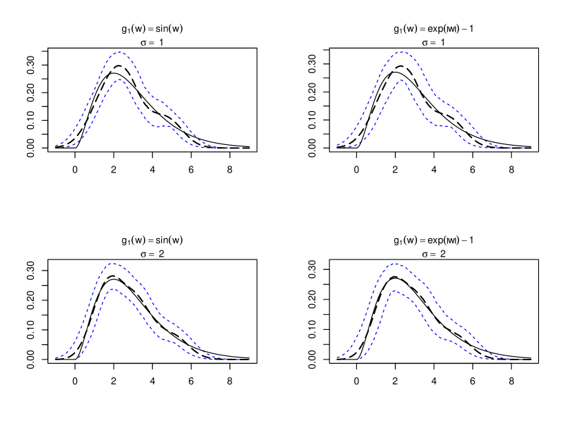
Figure 4: As in Figure 2 but where the true density, depicted as solid line, is the density of $\Gamma(3,1)$ and $A_{0}\sim\mathcal{U}(0,1)$. Estimators are normalized to integrate to one.

4.2 An Empirical Illustration

In this subsection, the methodology is applied to analyze heterogeneity in income elasticity of demand for housing. Heterogeneity plays an important role in classical consumer demand and might be driven by unobserved heterogenous preferences. In the empirical illustration we use data from the German Socio-Economic Panel (SOEP). While the SOEP is a longitudinal survey we restrict ourselves to the year 2013. We only consider individuals who do not have missing observations in rent, income, and size of the apartment, which results in a sample of size $n=7230$.

We are interested in assessing the heterogenous effect of household income on households’ willingness to pay for rent. Formally, let us consider the empirical VRC model

$$Y=B_{1}X+g_{0}(W)+A_{0},$$

and

$$B_{1}=g_{1}(W)+A_{1},$$

where $Y$ denotes the log monthly rent, $X$ denotes the logarithm of the household net income per month, and $W$ is the logarithm of the size of the housing unit in square meters. The empirical VRC model thus imposes functional forms rather than letting the conditional distribution of unobserved heterogeneity given housing characteristics unrestricted. The following table provides summary statistics of the relevant variables.

	Min.	1st Qu.	Median	Mean	3rd Qu.	Max.	St. Dev.
$Y$: log rent	2.485	5.858	6.120	6.113	6.389	8.517	0.444
$X$: log hh. income	5.193	7.162	7.550	7.520	7.901	10.130	0.569
$W$: log size housing	2.303	4.060	4.263	4.253	4.477	5.886	0.371

The interpretation of $B_{1}$ is that of a heterogeneous elasticity. Independence of the heterogeneous income elasticity of demand and income itself might be difficult to justify if no additional covariates are included to explain $B_{1}$. We compute the variance of $B_{1}$ from the empirical analog of $\operatorname{\mathbb{E}}[(Y-g_{1}(W))^{2}X]-\operatorname{\mathbb{E}}[(Y-g_{1}(W))X]^{2}$ which yields the value of $0.0431$, where $g_{1}$ is estimated using B-splines as described below. The log size of housing $W$ explains much of the variation in $B_{1}$, i.e., if $g_{1}\equiv 0$ then variance of $B_{1}$ is given by $0.5899$. The small variance does not prevent estimating the density of $B_{1}$ using global basis functions, such as Hermite functions, because we can transform the model such that $B_{1}$ has , e.g., variance one and then back–transform the density function of $B_{1}$. Here, $g_{1}$ is replaced by a B-spline estimator as explained below.

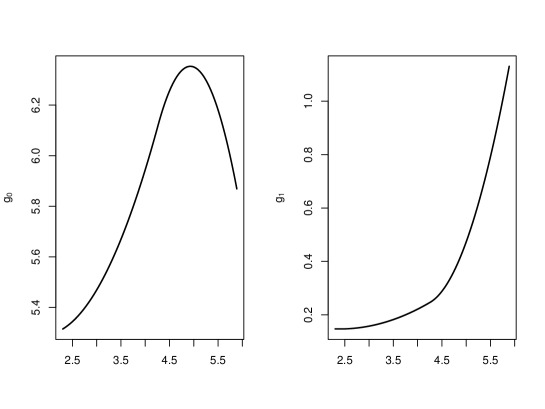
Figure 5: Left: B-spline estimator of $g_{0}$. Right: B-spline estimator of $g_{1}$.

The estimator $\widehat{f}_{B_{1}}$ is implemented as described in the previous section. The number of Hermite functions used is $K_{0}=1$ and $K_{1}=7$. The weighting measure $\nu$ is again given by $\textsl{Lognormal}(0,\sigma_{\nu}^{2})$ with $\sigma_{\nu}=1/4$, as in the Monte Carlo section. For estimation of the functions $g_{0}$ and $g_{1}$ we use again quadratic B-spline bases functions with three interior knots and follow Example 3.2. Figure 5 depicts the B-spline estimators for the varying coefficient functions $g_{0}$ and $g_{1}$. We see that both estimators are nonlinear on the support of $W$.

For the bootstrap uniform confidence bands, we consider one representative sample and generate the bootstrap innovations $\varepsilon$ according to the two-point distribution suggested by Mammen [1993], i.e., $\varepsilon$ equals $(1-\sqrt{5})/2$ with probability $(1+\sqrt{5})/(2\sqrt{5})$ and $(1+\sqrt{5})/2$ with probability $1-(1+\sqrt{5})/(2\sqrt{5})$. Based on the estimator we generate the bootstrap process $\mathbb{Z}^{*}(\cdot|w)$ as described in Subsection 3.4. The results are based on $1000$ bootstrap iterations.

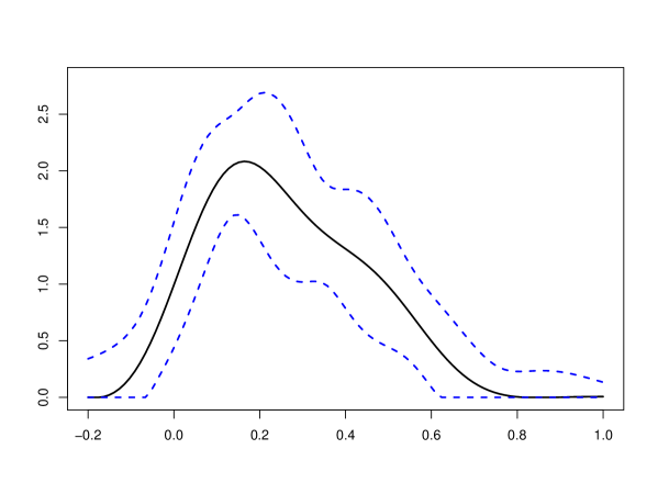
Figure 6: Solid line depicts the sieve estimator of $f_{B_{1}}$ based on $K_{1}=7$ Hermite functions. Dotted lines depict the $95\%$ uniform confidence bands based on $1000$ bootstrap iterations.

Figure 6 depicts the estimator for the density of $B_{1}$ evaluated at the mean of $W$ which is $w=4.253$. Note that $B_{1}$ can be directly interpreted as heterogenous marginal effect. From this figure we see that the estimated density has support between $-0.2$ and $0.8$. The uniform confidence bands show that the support is significantly positive (at $0.05$ nominal level) only at $-0.05$ and $0.6$. The estimated density is clearly not symmetric. We also see that the density is positively skewed and is more heavy tailed on the right hand side. This is reasonable as one would expect the response of a marginal increase of income to be skewed. It is also interesting to see that the $95\%$ uniform confidence sets are bounded away from zero.

5 Conclusion

This paper analyzes heterogeneity in VRC models. This model generalizes ordinary RC models by including nonlinearities in observed characteristics, which might stem, for instance, from measurement errors or control function residuals. A novel estimator of the VRC density based on weighted sieve minimum distance is proposed. Under semiparametric restrictions on the random intercept, our estimator of the VRS density is not affected by the ill-posedness that is associated with the nonparametric estimation of the joint VRC density. We establish novel inference results, such as uniform confidence bands, to adress uncertainty in VRC density estimation which goes beyond what has been shown in ordinary RC models. We find that finite sample estimation results are surprisingly stable when the sieve space is spanned by Hermite functions. This also advocates the use of the proposed methodology in the context of ordinary RC models. Finally, the methodology is applied to estimate the density of heterogeneous income elasticity of demand for housing, which is shown to be highly skewed. The proposed estimator can also be extended to include nonlinear index functions as in Lewbel and Pendakur [2017]. Yet the analysis of its asymptotic properties is left to future research.

Appendix A Appendix

Throughout the proofs, we will use $C>0$ to denote a generic finite constant that may be different in different uses. Further, for ease of notation we write $\sum_{j}$ for $\sum_{j=1}^{n}$ and $\int$ for $\int_{\mathbb{R}^{d}}$ or $\int_{\mathbb{R}^{d-1}}$. Recall that $\|\cdot\|$ denotes the usual Euclidean norm, while for a matrix $A$, $\|A\|$ is the operator norm. Recall the notation $P=\operatorname{\mathbb{E}}[p^{K}(X)p^{K}(X)^{\prime}]$ and $\widehat{P}=n^{-1}\sum_{j}p^{K}(X_{j})p^{K}(X_{j})^{\prime}$. We use the notation $a_{n}\lesssim b_{n}$ to denote $a_{n}\leq Cb_{n}$ for all $n\geq 1$.

Proof of Lemma 2.1..

The VRC model $(\ref{mod:gen}$–$\ref{mod:gen:rc})$ yields by Assumption 1 (ii) the conditional moment restriction $\operatorname{\mathbb{E}}[Y|X,W]=g_{0}(W)+\sum_{l=1}^{d-1}g_{l}(W)X_{l}$. The varying coefficients functions $g_{l}$, $0\leq l\leq d-1$, are identified through this conditional moment restriction by Assumption 1 (iii) . Further, we obtain

$$\operatorname{\mathbb{E}}[\exp(it(Y-g(S)))|X=x]=\operatorname{\mathbb{E}}[\exp(it(A_{0}+A_{1}^{\prime}X))|X=x].$$

Since $X$ is independent of $A$ (see Assumption Assumption 1 (i)) we can rewrite this equation using the notation of the Fourier transform for any $x$ in the support of $X$ as

$$h(x,t;g)=(\mathcal{F}f_{A})(t,tx).$$

By the large support condition imposed on $X$ in Assumption 1 (i) we can make use of Fourier inversion to obtain

$$f_{A}(a) =\frac{1}{(2\pi)^{d}}\int\exp(-ia^{\prime}u)(\mathcal{F}f_{A})(u)du$$

$$=\frac{1}{(2\pi)^{d}}\int\int|t|^{d-1}\exp\big{(}-it(1,x^{\prime})a\big{)}(\mathcal{F}f_{A})(t,tx)dt\,dx$$

$$=\frac{1}{(2\pi)^{d}}\int\int|t|^{d-1}\exp\big{(}-it(1,x^{\prime})a\big{)}h(x,t;g)dt\,dx,$$

where the integral on the right hand side is finite due to Assumption 1 (ii). This shows identification of the RC density $f_{A}$ of $A$. Now identification of the VRC density of $B^{w}=\mathbf{g}(w)+A$ follows immediately by employing the relationship $f_{B}(b,w)=f_{A}(b-\mathbf{g}(w))$. ∎

Proof of Lemma 3.1..

From the formula of the double series least squares estimator with $Q$ given in (3.5) and from basic properties of the Kronecker product we infer

$$Q =(2\pi)^{d/2}\int\int\Big{(}\widetilde{q}^{K_{0}}(-t)\otimes\widetilde{q}^{K_{1}}(-tx)\Big{)}\Big{(}\widetilde{q}^{K_{0}}(t)\otimes\widetilde{q}^{K_{1}}(tx)\Big{)}^{\prime}d\nu(t)dx$$

$$=(2\pi)^{d/2}\int\int\widetilde{q}^{K_{0}}(-t)\widetilde{q}^{K_{0}}(t)^{\prime}\otimes\widetilde{q}^{K_{1}}(-tx)\widetilde{q}^{K_{1}}(tx)^{\prime}d\nu(t)dx$$

$$=(2\pi)^{d/2}\int|t|^{1-d}\widetilde{q}^{K_{0}}(-t)\widetilde{q}^{K_{0}}(t)^{\prime}d\nu(t)\otimes\int\widetilde{q}^{K_{1}}(-u)\widetilde{q}^{K_{1}}(u)^{\prime}du$$

$$=(2\pi)^{d/2}\int|t|^{1-d}\widetilde{q}^{K_{0}}(-t)\widetilde{q}^{K_{0}}(t)^{\prime}d\nu(t)\otimes\text{I}_{K_{1}}$$

using that $q^{K_{1}}$ is a vector of Hermite functions which are orthonormal in $L^{2}(\mathbb{R}^{d-1})$. ∎

Proof of Proposition 3.2..

Proof of (i). Recall the definition $\widetilde{\nu}(t)=|t|^{1-d}\nu(t)$. For some constant $0<c<1$, for all $n\geq 1$, and any $a\in\mathbb{R}^{K}$ we have due to Parseval’s Formula:

$$\|a\|^{2} =\int\int|a^{\prime}\,q^{K}(t,u)|^{2}du\,dt$$

$$=\int\int|a^{\prime}\,(\mathcal{F}q^{K})(t,u)|^{2}du\,dt$$

$$=\int\int|a^{\prime}\,(\mathcal{F}q^{K})(t,tx)|^{2}\,|t|^{d-1}\mathop{\mathbbm{1}}\nolimits\{\widetilde{\nu}(t)\geq\tau_{K}\}dx\,dt$$

$$\quad+\int\int|a^{\prime}\,(\mathcal{F}q^{K})(t,u)|^{2}\mathop{\mathbbm{1}}\nolimits\{\widetilde{\nu}(t)<\tau_{K}\}du\,dt$$

$$\leq\tau_{K}^{-1}\int\int|a^{\prime}\,(\mathcal{F}q^{K})(t,tx)|^{2}\,|t|^{d-1}dx\,d\widetilde{\nu}(t)+c\int\int|a^{\prime}\,(\mathcal{F}q^{K})(t,u)|^{2}du\,dt$$

$$=\tau_{K}^{-1}\int\int|a^{\prime}\,(\mathcal{F}q^{K})(t,tx)|^{2}dx\,d\nu(t)+c\,\|a\|^{2}.$$

Consequently, we obtain $\tau_{K}\text{I}_{K}\lesssim Q$.

Proof of (ii). Using the series expansion of $f$ given by $f=\sum_{k\geq 1}\langle f,q_{k}\rangle_{\mathbb{R}^{d}}q_{k}$ we obtain by the Cauchy-Schwarz inequality

$$\int \int\big{|}[\mathcal{F}(\Pi_{K}f-f)](t,tx)\big{|}^{2}dx\,d\nu(t)=\int\int\Big{|}\sum_{k\geq K}\langle f,q_{k}\rangle_{\mathbb{R}^{d}}(\mathcal{F}q_{k})(t,tx)\Big{|}^{2}dx\,d\nu(t)$$

$$\leq\Big{(}\sum_{k\geq K}\langle f,q_{k}\rangle_{\mathbb{R}^{d}}^{2}\Big{)}\,\Big{(}\sum_{k\geq K}\int\int|(\mathcal{F}q_{k})(t,tx)|^{2}dx\,d\nu(t)\Big{)}$$

$$=\int(\Pi_{K}f-f)^{2}(b)\,db\,\sum_{k\geq K}\int\int|(\mathcal{F}q_{k})(t,u)|^{2}du\,d\widetilde{\nu}(t)$$

$$=\int(\Pi_{K}f-f)^{2}(b)\,db\,\sum_{k\geq K}\int|(\mathcal{F}q_{k})(t)|^{2}d\widetilde{\nu}(t),$$

by the unitary property of the Fourier transform, which completes the proof. ∎

For the following proofs we require additional notation. Introduce the vector

$$\psi^{K}(Y_{j},S_{j};\phi,t)=\big{(}\exp(it(Y_{j}-\phi(S_{j})))-\exp(it(Y_{j}-g(S_{j})))\big{)}\widetilde{p}^{K}(X_{j})$$ (A.1)

with $k$–th entry denoted by $\psi_{k}(Y_{j},S_{j};\phi,t)$ and $\widetilde{p}^{K}(\cdot):=P^{-1/2}p^{K}(\cdot)$. We also introduce the classes of function $\mathcal{G}=\{\phi=\beta^{\prime}p_{d}^{K}:\|\phi-g\|_{\infty}\leq\sqrt{K/n}\}$, $\mathcal{F}_{k}^{R}=\{\text{Re}(\psi_{k}(\cdot;\phi,\cdot)):\,\phi\in\mathcal{G}\}$, and $\mathcal{F}_{k}^{I}=\{\text{Im}(\psi_{k}(\cdot;\phi,\cdot)):\,\phi\in\mathcal{G}\}$. Further, $N_{[\,]}(\mathcal{F},\|\cdot\|_{\nu,2},\epsilon)$ denotes the $\|\cdot\|_{\nu,2}:=\sqrt{\int\|\cdot\|_{YS}^{2}\,d\nu}$ covering number with bracketing of a set of function $\mathcal{F}$. Define the envelope function $\Psi_{k}(\cdot)=\sup_{\phi\in\mathcal{G}}|\psi_{k}(\cdot;\phi,\cdot)|$, which satisfies

$$\max_{1\leq k\leq K}\operatorname{\mathbb{E}}\int|\Psi_{k}(Y,S;t)|^{2}d\nu(t) \leq\max_{1\leq k\leq K}\operatorname{\mathbb{E}}\big{[}\sup_{\phi\in\mathcal{G}}\big{|}\big{(}\phi(S)-g(S)\big{)}\widetilde{p}_{k}(X)\big{|}^{2}\big{]}\int t^{2}d\nu(t)$$

$$\leq\sup_{\phi\in\mathcal{G}}\|\phi-g\|_{\infty}^{2}\max_{1\leq k\leq K}\operatorname{\mathbb{E}}[\widetilde{p}_{k}^{2}(X)]\int t^{2}d\nu(t)$$

$$\lesssim K/n,$$ (A.2)

using $\int t^{2}d\nu(t)\lesssim 1$ by Assumption 3 (ii). This upper bound is used in the following proofs.

Proof of Theorem 3.1..

The proof is based on the decomposition

$$\int\big{|}\widehat{f}_{B}(b,w)-f_{B}(b,w)\big{|}^{2}db \lesssim\int\big{|}\widehat{f}_{A}(a)-f_{A}(a)\big{|}^{2}da$$

$$\quad+\int\big{|}f_{A}\big{(}a-\widehat{\mathbf{g}}(w)\big{)}-f_{A}\big{(}a-\mathbf{g}(w)\big{)}\big{|}^{2}da$$

$$\lesssim\int\big{|}\widehat{f}_{A}(a)-\Pi_{K}f_{A}(a)\big{|}^{2}da+\int\big{|}\Pi_{K}f_{A}(a)-f_{A}(a)\big{|}^{2}da$$

$$\quad+\int\big{|}f_{A}\big{(}a-\widehat{\mathbf{g}}(w)\big{)}-f_{A}\big{(}a-\mathbf{g}(w)\big{)}\big{|}^{2}da.$$ (A.3)

Consider the first summand on the right hand side. We have

$$\sup_{f\in\mathcal{A}_{K}}{\left\{\frac{\int f^{2}(b)db}{\int\int|(\mathcal{F}f)(t,tx)|^{2}d\nu(t)\,dx}\right\}}\lesssim\tau_{K}^{-1},$$ (A.4)

which is a consequence of the upper bounds imposed in Assumption 3, that is, $\lambda_{\max}(\tau_{K}Q^{-1})\lesssim 1$ and $\lambda_{\max}\big{(}\int q^{K}(a)q^{K}(a)^{\prime}da\big{)}\lesssim 1$, since for any $f(\cdot)=\beta^{\prime}q^{K}(\cdot)$ it holds

$$\int\int|(\mathcal{F}f)(t,tx)|^{2}d\nu(t)\,dx =\beta^{\prime}\,\int\int(\mathcal{F}q^{K})(t,tx)(\mathcal{F}q^{K})(t,tx)^{\prime}dx\,d\nu(t)\,\beta$$

$$\gtrsim\tau_{K}\|\beta\|^{2}$$

$$\gtrsim\tau_{K}\int f^{2}(b)db.$$

The definition of the estimator $\widehat{f}_{A}$ implies

$$\int\int\Big{|}\widehat{h}(x,t;\widehat{g})-(\mathcal{F}\widehat{f}_{A})(t,tx)\Big{|}^{2}d\nu(t)\,dx\\ \leq\int\int\Big{|}\widehat{h}(x,t;\widehat{g})-(\mathcal{F}\Pi_{K}f_{A})(t,tx)\Big{|}^{2}d\nu(t)\,dx.$$

This inequality, the upper bound (A.4), and the definition of the estimator $\widehat{h}$ yield

$$\tau_{K}\int\big{|}\widehat{f}_{A}(a)-\Pi_{K}f_{A}(a)\big{|}^{2}da\lesssim\int\int\Big{|}(\mathcal{F}\widehat{f}_{A})(t,tx)-(\mathcal{F}\Pi_{K}f_{A})(t,tx)\Big{|}^{2}d\nu(t)\,dx$$

$$\lesssim\int\int\Big{|}\widehat{h}(x,t;\widehat{g})-(\mathcal{F}\Pi_{K}f_{A})(t,tx)\Big{|}^{2}d\nu(t)\,dx$$

$$\lesssim\underbrace{\int\int\Big{|}(\mathcal{F}f_{A}-\mathcal{F}\Pi_{K}f_{A})(t,tx)\Big{|}^{2}d\nu(t)\,dx}_{I}$$

$$+\underbrace{\int\int\Big{|}p^{K}(x)^{\prime}\widehat{P}^{-1}\frac{1}{n}\sum_{j}\exp\big{(}it(Y_{j}-g(S_{j}))\big{)}p^{K}(X_{j})-p^{K}(x)^{\prime}\gamma(t)\Big{|}^{2}d\nu(t)\,dx}_{II}$$

$$+\underbrace{\int\int\Big{|}p^{K}(x)^{\prime}\widehat{P}^{-1}\frac{1}{n}\sum_{j}\exp(itY_{j})p^{K}(X_{j})\big{(}\exp\big{(}it\,\widehat{g}(S_{j})\big{)}-\exp\big{(}it\,g(S_{j})\big{)}\big{)}\Big{|}^{2}d\nu(t)\,dx}_{III}$$

$$+\underbrace{\int\int\Big{|}p^{K}(x)^{\prime}\gamma(t)-h(x,t;g)\Big{|}^{2}d\nu(t)\,dx}_{IV}.$$

Due to the sieve approximation error of $f_{A}$ in Assumption 4 (i) it holds

$$I=\|\mathcal{F}\Pi_{K}f_{A}-\mathcal{F}f_{A}\|_{\nu}^{2}=O\Big{(}\tau_{K}\|\Pi_{K}f_{A}-f_{A}\|_{\mathbb{R}^{d}}^{2}\Big{)}=\tau_{K}K^{-2\zeta/d}.$$

In the following, we make use of $\|\widehat{P}^{-1}-P^{-1}\|=O_{p}(\lambda_{K}^{-1}\sqrt{K\log(n)/n})$, see [Belloni et al., 2015, Lemma 6.2] or [Chen and Christensen, 2015, Lemma 2.1]. By Assumption 3 (iii), the eigenvalues of $\int p^{K}(x)p^{K}(x)^{\prime}dx$ are bounded from above and thus

$$II \leq\Big{\|}\int p^{K}(x)p^{K}(x)^{\prime}dx\Big{\|}\,\big{\|}\widehat{P}^{-1}P^{1/2}\big{\|}^{2}$$

$$\quad\times\int\Big{\|}n^{-1}\sum_{j}\Big{(}\exp\big{(}it(Y_{j}-g(S_{j}))\big{)}-p^{K}(X_{j})^{\prime}\gamma(t)\Big{)}\widetilde{p}^{K}(X_{j})\Big{\|}^{2}d\nu(t)$$

$$\lesssim\lambda_{K}^{-1}\int\Big{\|}\operatorname{\mathbb{E}}\Big{[}\big{(}h(X,t;g)-p^{K}(X)^{\prime}\gamma(t)\big{)}\widetilde{p}^{K}(X)\Big{]}\Big{\|}^{2}d\nu(t)+O_{p}(K/(n\lambda_{K}))$$

$$\lesssim\lambda_{K}^{-1}\int\operatorname{\mathbb{E}}\big{|}h(X,t;g)-p^{K}(X)^{\prime}\gamma(t)\big{|}^{2}d\nu(t)+O_{p}(K/(n\lambda_{K}))$$

$$=O_{p}\big{(}\lambda_{K}^{-1}K^{-2\rho/(d-1)}+K/(n\lambda_{K})\big{)},$$

making use of the sieve approximation condition imposed on Assumption 4 (i). Consider $III$. Due to Assumption 4 (iii) we may assume $\widehat{g}\in\mathcal{G}$, which implies

$$III \lesssim\int\int\sup_{\phi\in\mathcal{G}}\Big{|}p^{K}(x)^{\prime}\widehat{P}^{-1}P^{1/2}n^{-1}\sum_{j}\psi^{K}(Y_{j},S_{j};\phi,t)\Big{|}^{2}d\nu(t)dx$$

by using the definition of $\psi^{K}$ as given in (A.1). Applying Theorem 2.14.5 of van der Vaart and Wellner [2000] together with the upper bound for the envelope function (A) yields

$$\sum_{k=1}^{K}\int\operatorname{\mathbb{E}}\sup_{\phi\in\mathcal{G}}\Big{|}n^{-1}\sum_{j}\psi_{k}(Y_{j},S_{j};\phi,t)-\operatorname{\mathbb{E}}\psi_{k}(Y,S;\phi,t)\Big{|}^{2}d\nu(t)$$

$$\lesssim\frac{1}{n}\sum_{k=1}^{K}\Big{(}\int\operatorname{\mathbb{E}}\sup_{\phi\in\mathcal{G}}\Big{|}n^{-1/2}\sum_{j}\psi_{k}(Y_{j},S_{j};\phi,t)-\operatorname{\mathbb{E}}\psi_{k}(Y,S;\phi,t)\Big{|}d\nu(t)\sqrt{\frac{K}{n}}+\sqrt{\frac{K}{n}}\Big{)}^{2}$$

$$\lesssim\frac{1}{n}\sum_{k=1}^{K}\Big{(}\int_{0}^{1}\sqrt{1+\log N_{[\,]}(\mathcal{F}_{k}^{R},\|\cdot\|_{\nu,2},\epsilon)}d\epsilon\,\sqrt{\frac{K}{n}}$$

$$\qquad\qquad\qquad\qquad+\int_{0}^{1}\sqrt{1+\log N_{[\,]}(\mathcal{F}_{k}^{I},\|\cdot\|_{\nu,2},\epsilon)}d\epsilon\,\sqrt{\frac{K}{n}}+\sqrt{\frac{K}{n}}\Big{)}^{2}$$

where the second upper bound is due to the last display of Theorem 2.14.2 of van der Vaart and Wellner [2000]. The upper bound of the envelope function in inequality (A) (implying local uniform $\|\cdot\|_{\nu,2}$ continuity of $\psi_{k}(\cdot;\phi,\cdot)$ with respect to $\phi\in\mathcal{G}$) together with Lemma 4.2 of Chen [2007] yields

$$\log N_{[\,]}(\mathcal{F}_{k}^{R},\|\cdot\|_{\nu,2},\epsilon)\leq\log N\big{(}\mathcal{G},\|\cdot\|_{S},\epsilon/4\big{)}.$$ (A.5)

Using Assumption 4 (iv) we thus obtain the rate $K/n$. Further, from the inequality $\lambda_{\max}(P^{-1/2}\int p^{K}(x)p^{K}(x)^{\prime}dxP^{-1/2})\lesssim\lambda_{K}^{-1}$ we infer

$$\int\int \sup_{\phi\in\mathcal{G}}\Big{|}p^{K}(x)^{\prime}P^{-1/2}\operatorname{\mathbb{E}}\psi^{K}(Y,S;\phi,t)\Big{|}^{2}d\nu(t)dx$$

$$\lesssim\lambda_{K}^{-1}\int\sup_{\phi\in\mathcal{G}}\operatorname{\mathbb{E}}\Big{|}\exp(it(Y-\phi(S)))-\exp(it(Y-g(S)))\Big{|}^{2}d\nu(t)$$

$$\lesssim\lambda_{K}^{-1}\sup_{\phi\in\mathcal{G}}\|\phi-g\|_{S}^{2}\int t^{2}d\nu(t)$$

$$=o_{p}\big{(}K/(n\lambda_{K})\big{)},$$

using $\operatorname{\mathbb{E}}|\exp(it(Y-\phi(S)))-\exp(it(Y-g(S)))|^{2}\leq t^{2}\|\phi-g\|_{S}^{2}$ and $\int t^{2}d\nu(t)\lesssim 1$ by Assumption 3 (ii). Moreover, by Assumption 4 we have the sieve approximation bias

$$IV=\|h-\gamma^{\prime}p^{K}\|_{\nu}^{2}\lesssim K^{-2\rho/(d-1)}.$$

In what follows, $Df$ denotes the Jacobian matrix of a function $f$. Finally, we consider

$$\int\big{|}f_{A} (b-\widehat{\mathbf{g}}(w))-f_{A}(b-{\mathbf{g}}(w))\big{|}^{2}db$$

$$=\int\Big{\|}\int_{0}^{1}Df_{A}\Big{(}b-u\,\widehat{\mathbf{g}}(w)+(u-1)\,\mathbf{g}(w)\Big{)}du\Big{\|}^{2}db\,\big{\|}\widehat{\mathbf{g}}(w)-\mathbf{g}(w)\big{\|}^{2}$$

Continuity of $Df_{A}$ and consistency of $\widehat{\mathbf{g}}$ implies

$$\int\Big{\|}\int_{0}^{1}Df_{A}\Big{(}b-u\,\widehat{\mathbf{g}}(w)+(u-1)\,\mathbf{g}(w)\Big{)}du\Big{\|}^{2}db =\int\|Df_{A}(a)\|^{2}da+o_{p}(1)$$

$$\lesssim 1+o_{p}(1).$$

The result follows due to the rate restriction imposed in Assumption 4 (iii). ∎

Proof of Theorem 3.2..

We make use of the notation $\beta=\int q^{K}(a)f_{A_{1}}(a)da$ where $q^{K}(t,u)=q^{K_{0}}(t)\otimes q^{K_{1}}(u)$. In light of the main decomposition (A) in the proof of Theorem 3.1 it is sufficient to consider

$$\int|\widehat{f}_{A_{1}}(a)-f_{A_{1}}(a)|^{2}da$$

$$\lesssim\Big{\|}\int\int b_{K_{0}}(t)\widetilde{q}^{K_{1}}(-tx)\widehat{h}(x,t;\widehat{g})d\nu(t)\,dx-\int\beta^{\prime}(q^{K_{0}}(a_{0})\otimes\text{I}_{K_{1}})da_{0}\Big{\|}^{2}$$

$$\quad+\int\Big{|}\int\beta^{\prime}(q^{K_{0}}(a_{0})\otimes q^{K_{1}}(a_{1}))-f_{A}(a_{0},a_{1})da_{0}\Big{|}^{2}da_{1}$$

$$\lesssim\Big{\|}Q^{-1}\int\int\big{(}\widetilde{q}^{K_{0}}(-t)\otimes\widetilde{q}^{K_{1}}(-tx)\big{)}\widehat{h}(x,t;\widehat{g})d\nu(t)\,dx-\beta\Big{\|}^{2}$$

$$\quad+\int\big{|}\beta^{\prime}(q^{K_{0}}(a_{0})\otimes q^{K_{1}}(a_{1}))-f_{A}(a_{0},a_{1})\big{|}^{2}d(a_{0},a_{1}),$$

using the notation $b_{K_{0}}(t)=\int q^{K_{0}}(a)^{\prime}Q_{0}^{-1}\widetilde{q}^{K_{0}}(-t)da$ and Lemma 3.1, that is, $Q^{-1}=Q_{0}^{-1}\otimes\text{I}_{K_{1}}$. Since $\int|\beta^{\prime}q^{K}(a)-f_{A}(a)|^{2}da=O(K_{1}^{-2\zeta/(d-1)})$ due to condition $K_{0}=O(1)$, we only need to bound the first term on the right hand side. We further observe

$$\beta =\int q^{K}(a)f_{A}(a)\,d(a)$$

$$=Q^{-1}\int\int\widetilde{q}^{K}(-t,-tx)(\mathcal{F}f_{A})(t,tx)d\nu(t)\,dx$$

$$=Q^{-1}\int\int\widetilde{q}^{K}(-t,-tx)h(x,t;g)d\nu(t)\,dx.$$

Therefore, it is sufficient to show

$$\Big{\|}Q_{1}^{-1}\int\int\widetilde{q}^{K}(-t,-tx)\big{(}\widehat{h}(x,t;\widehat{g})-h(x,t;g)\big{)}d\nu(t)\,dx\Big{\|}^{2}=O_{p}\big{(}K_{1}/(n\lambda_{K_{1}})\big{)}.$$

This upper bound follows immediately from the proof of Theorem 3.1 by using that $K_{1}$ is the dimension of basis functions used for the estimator $\widehat{h}$ and that $K_{0}=O(1)$, which completes the proof. ∎

Proof of Theorem 3.3..

To simplify notation, let $\mathbf{s}:=Q^{-1/2}\ell\big{(}q^{K}(\cdot-\mathbf{g}(w))\big{)}$. Making use of Assumption 5 (i), we obtain the following lower bound for the sieve variance

$$\textsl{v}_{K}(w)=\mathbf{s}^{\prime}\,\Sigma\,\mathbf{s}\gtrsim\lambda_{K}^{-1}\|\mathbf{s}\|^{2}$$

which is used throughout this proof. The proof is based on the decomposition

$$\ell\big{(}\widehat{f}_{B}(\cdot,w)\big{)} -\ell\big{(}f_{B}(\cdot,w)\big{)}=\underbrace{\ell\big{(}\widehat{f}_{A}(\cdot-{\widehat{\mathbf{g}}}(w))\big{)}-\ell\big{(}\widehat{f}_{A}(\cdot-{{\mathbf{g}}}(w))\big{)}}_{I}$$

$$+\underbrace{\mathbf{s}^{\prime}Q^{-1/2}\int\int(\mathcal{F}q^{K})(-t,-tx)\Big{(}\widehat{h}(x,t;\widehat{g})-\widehat{h}(x,t;g)\Big{)}d\nu(t)dx}_{II}$$

$$+\underbrace{\mathbf{s}^{\prime}Q^{-1/2}\int\int(\mathcal{F}q^{K})(-t,-tx)\Big{(}\widehat{h}(x,t;g)-p^{K}(x)^{\prime}\gamma(t)\Big{)}d\nu(t)dx}_{III}$$

$$+\underbrace{\mathbf{s}^{\prime}Q^{-1/2}\int\int(\mathcal{F}q^{K})(-t,-tx)\Big{(}p^{K}(x)^{\prime}\gamma(t)-h(x,t;g)\Big{)}d\nu(t)dx}_{IV}$$

$$+\underbrace{\mathbf{s}^{\prime}Q^{-1/2}\int\int(\mathcal{F}q^{K})(-t,-tx)(\mathcal{F}f_{A})(t,tx)d\nu(t)dx-\ell\big{(}f_{B}(\cdot,w)\big{)}}_{V},$$

where we evaluate each summand separately in the following. By Assumption 5 (iv) the basis functions $q_{l}$ are continuously differentiable and thus

$$\sqrt{n}\,I \leq\sqrt{n}\,\Big{\|}\ell\Big{(}\int_{0}^{1}D\widehat{f}_{A}\big{(}\cdot-u\,{\widehat{\mathbf{g}}}(w)+(u-1)\,{\mathbf{g}}(w)\big{)}du\Big{)}\Big{\|}\,\big{\|}{\widehat{\mathbf{g}}}(w)-{\mathbf{g}}(w)\big{\|}$$

$$=o_{p}\Big{(}\sqrt{\textsl{v}_{K}(w)}\Big{)}$$

using that $n\|\widehat{\mathbf{g}}(w)-\mathbf{g}(w)\|^{2}=o_{p}\big{(}\textsl{v}_{K}(w)\big{)}$, consistency of $\widehat{f}_{A}$, and Assumption 4 (ii). To bound $II$, make use of the definition of $\psi^{K}$ as given in (A.1) to obtain

$$\sqrt{n}\,II$$

$$=\mathbf{s}^{\prime}\int R(t)\widehat{P}^{-1}\frac{1}{\sqrt{n}}\sum_{j}\exp\big{(}itY_{j})\Big{(}\exp\big{(}-it\widehat{g}(S_{j})\big{)}-\exp\big{(}-itg(S_{j})\big{)}\Big{)}p^{K}(X_{j})d\nu(t)$$

$$\lesssim\int\sup_{\phi\in\mathcal{G}}\Big{|}\mathbf{s}^{\prime}R(t)\widehat{P}^{-1}P^{1/2}\frac{1}{\sqrt{n}}\sum_{j}\psi^{K}(Y_{j},S_{j};\phi,t)\Big{|}d\nu(t)$$

$$\lesssim\Big{(}\int\Big{\|}\mathbf{s}^{\prime}R(t)P^{-1/2}\Big{\|}^{2}d\nu(t)\Big{)}^{1/2}$$

$$\qquad\times\Big{(}\int\sup_{\phi\in\mathcal{G}}\Big{\|}\frac{1}{\sqrt{n}}\sum_{j}\Big{(}\psi^{K}(Y_{j},S_{j};\phi,t)-\operatorname{\mathbb{E}}\psi^{K}(Y,S;\phi,t)\Big{)}\Big{\|}^{2}d\nu(t)\Big{)}^{1/2}$$

$$\quad+\sqrt{n}\int\sup_{\phi\in\mathcal{G}}\Big{|}\mathbf{s}^{\prime}R(t)P^{-1/2}\operatorname{\mathbb{E}}\psi^{K}(Y,S;\phi,t)\Big{|}d\nu(t)+o_{p}(1).$$

Assumption $\int\|R(t)\|^{2}d\nu(t)=O(1)$ implies

$$\int\Big{\|}\mathbf{s}^{\prime}R(t)P^{-1/2}\Big{\|}^{2}d\nu(t) \leq\|\mathbf{s}\|^{2}\int\|R(t)\|^{2}d\nu(t)\|P^{-1/2}\|^{2}$$

$$\lesssim\textsl{v}_{K}(w).$$

Making use of the upper bound (A) for the envelope function of $\mathcal{F}^{R}_{k}$ and $\mathcal{F}^{I}_{k}$ and applying Theorem 2.14.5 of van der Vaart and Wellner [2000] yields

$$\sum_{l=1}^{K}\int\operatorname{\mathbb{E}}\sup_{\phi\in\mathcal{G}}\Big{|}n^{-1/2}\sum_{j}\psi_{l}(Y_{j},S_{j};\phi,t)-\operatorname{\mathbb{E}}\psi_{l}(Y,S;\phi,t)\Big{|}^{2}d\nu(t)$$

$$\lesssim\sum_{l=1}^{K}\Big{(}\int\operatorname{\mathbb{E}}\sup_{\phi\in\mathcal{G}}\Big{|}n^{-1/2}\sum_{j}\psi_{l}(Y_{j},S_{j};\phi,t)-\operatorname{\mathbb{E}}\psi_{l}(Y,S;\phi,t)\Big{|}d\nu(t)\sqrt{K/n}$$

$$\qquad\qquad\qquad\qquad\qquad\qquad+\sqrt{K/n}\Big{)}^{2}$$

$$\lesssim\frac{K}{n}\sum_{k=1}^{K}\Big{(}\int_{0}^{1}\sqrt{1+\log N_{[\,]}(\mathcal{F}_{k}^{R},\|\cdot\|_{\nu,2},\epsilon)}d\epsilon$$

$$\qquad\qquad\qquad\qquad\qquad\qquad+\int_{0}^{1}\sqrt{1+\log N_{[\,]}(\mathcal{F}_{k}^{I},\|\cdot\|_{\nu,2},\epsilon)}d\epsilon+1\Big{)}^{2}$$

$$\lesssim C_{n}^{2}K^{2}/n$$

due to inequality (A.5) and Assumption 4 (iv). Further, we have

$$\int\operatorname{\mathbb{E}}\sup_{\phi\in\mathcal{G}} \Big{|}\mathbf{s}^{\prime}R(t)P^{-1/2}\operatorname{\mathbb{E}}\psi^{K}(Y,S;\phi,t)\Big{|}d\nu(t)$$

$$=\sup_{\phi\in\mathcal{G}}\|\phi-g\|_{S}\|\mathbf{s}\|\Big{(}\int\|R(t)\|^{2}d\nu(t)\Big{)}^{1/2}\|P^{-1/2}\|$$

$$\lesssim\sqrt{\textsl{v}_{K}(w)K/n}.$$

Consequently, the rate restriction imposed on $K$ implies $\sqrt{n}II=o(\sqrt{\textsl{v}_{K}(w)})$. Consider $III$. Note that $\widehat{P}\gamma(t)=n^{-1}\sum_{j}h(X_{j},t,g)p^{K}(X_{j})$ and consequently we obtain by the definition of $R(t)$ that

$$\sqrt{n}\,III =\mathbf{s}^{\prime}\int R(t)\,\widehat{P}^{-1}\frac{1}{\sqrt{n}}\sum_{j}\Big{(}\exp(it(Y_{j}-g(S_{j})))p^{K}(X_{j})-\widehat{P}\gamma(t)\Big{)}d\nu(t)$$

$$\quad+o_{p}(1)$$

$$=\mathbf{s}^{\prime}\int R(t)\,P^{-1}\frac{1}{\sqrt{n}}\sum_{j}\rho_{j}(t)p^{K}(X_{j})d\nu(t)+o_{p}(1),$$

where $\rho_{j}(t)=\exp(it(Y_{j}-g(S_{j})))-h(X_{j},t,g)$. Consequently, we obtain

$$\sqrt{n/\textsl{v}_{K}(w)}\,III =\sum_{j}\underbrace{\big{(}n\,\textsl{v}_{K}(w)\big{)}^{-1/2}\mathbf{s}^{\prime}\int R(t)\rho_{j}(t)d\nu(t)P^{-1}p^{K}(X_{j})}_{\zeta_{j}}+o_{p}(1).$$

We show $\sum_{j}\zeta_{j}\stackrel{{\scriptstyle d}}{{\rightarrow}}\mathcal{N}(0,1)$ by the Lindeberg-Feller theorem. We see below that $\zeta_{j}$, $1\leq j\leq n$ satisfy Lindeberg’s condition. It holds $\operatorname{\mathbb{E}}[\zeta_{j}]=0$ and $n\operatorname{\mathbb{E}}[\zeta_{j}^{2}]=1$. Using the lower bound for the sieve variance, for $\varepsilon>0$ we observe

$$\sum_{j} \operatorname{\mathbb{E}}[\zeta_{j}^{2}\mathop{\mathbbm{1}}\nolimits\{|\zeta_{j}|>\varepsilon\}]\leq n\varepsilon^{2}\operatorname{\mathbb{E}}|\zeta_{j}/\varepsilon|^{4}$$

$$\leq\textsl{v}_{K}(w)^{-2}n^{-1}\varepsilon^{-2}\|\mathbf{s}\|^{4}\operatorname{\mathbb{E}}\big{\|}\int R(t)\rho(t)d\nu(t)P^{-1}p^{K}(X)\big{\|}^{4}$$

$$\lesssim n^{-1}\lambda_{K}^{2}\Big{(}\int\|R(t)\|^{2}d\nu(t)\Big{)}^{2}\operatorname{\mathbb{E}}\Big{[}\Big{(}\int|\rho(t)|^{2}d\nu(t)\Big{)}^{2}\big{\|}P^{-1}p^{K}(X)\big{\|}^{2}\Big{]}$$

$$\qquad\times\sup_{x}\big{\|}P^{-1}p^{K}(x)\big{\|}^{2}$$

$$\lesssim n^{-1}\lambda_{K}^{-1}K^{2}$$

$$=o(1),$$

by the rate condition $K^{2}=o(n\lambda_{K})$ imposed in Assumption 5. Consider $IV$. Using the notation $\check{q}^{K}(t,tx)=Q^{-1/2}(\mathcal{F}q^{K})(t,tx)$ and linearity of the Fourier transform we obtain

$$IV =\mathbf{s}^{\prime}Q^{-1/2}\int\int(\mathcal{F}q^{K})(t,tx)\Big{(}p^{K}(x)^{\prime}\gamma(t)-h(x,t;g)\Big{)}d\nu(t)dx$$

$$=\sum_{l=1}^{K}\ell\Big{(}(\mathcal{F}^{-1}\check{q}_{l})(\cdot-\mathbf{g}(w))\Big{)}\langle\check{q}_{l},\gamma^{\prime}p^{K}-h\rangle_{\nu}$$

$$\lesssim\ell\big{(}[\mathcal{F}^{-1}(\gamma^{\prime}p^{K}-h)](\cdot-\mathbf{g}(w))\big{)}$$

$$=o\big{(}\sqrt{\textsl{v}_{K}(w)/n}\big{)},$$

by Assumption 5 (iii). Consider $V$. By Assumption 5 (iv) the sieve space $\mathcal{A}_{K}$ is linear and thus, it holds

$$V =\mathbf{s}^{\prime}Q^{-1/2}\int\int(\mathcal{F}q^{K})(t,tx)(\mathcal{F}f_{A})(t,tx)d\nu(t)\,dx-\ell\big{(}f_{B}(\cdot,w)\big{)}$$

$$=\mathbf{s}^{\prime}\underbrace{Q^{-1/2}\int\int(\mathcal{F}q^{K})(t,tx)[\mathcal{F}(f_{A}-\Pi_{K}f_{A})](t,tx)d\nu(t)\,dx}_{=0}$$

$$\quad+\ell\big{(}\Pi_{K}f_{A}(\cdot-\mathbf{g}(w))-f_{A}(\cdot-\mathbf{g}(w))\big{)}$$

$$=o\big{(}\sqrt{\textsl{v}_{K}(w)/n}\big{)},$$

by Assumption 5 (iii). Due to Lemma B.1, equation (B.1), the asymptotic distribution result remains valid as $\textsl{v}_{K}(w)$ is replaced by $\widehat{\textsl{v}}_{K}(w)$, which completes the proof. ∎

Proof of Theorem 3.4..

Due to the [Chen and Christensen, 2018, Proof of Theorem 4.1] it is sufficient to show

$$\left|\sqrt{n/\widehat{\textsl{v}}_{K}(b,w)}\big{(}\widehat{f}_{B}(b,w)-f_{B}(b,w)\big{)}-\mathbb{Z}(b,w)\right|=o_{p}(r_{n})$$

since then the result follows by the anti-concentration inequality of [Chernozhukov et al., 2014, Theorem 2.1]. Along the proof the inequality $\textsl{v}_{K}(b,w)\gtrsim\lambda_{K}^{-1}\|Q^{-1/2}q^{K}(b-\mathbf{g}(w))\|^{2}$. Let $Z^{n}=\{(Y_{1},X_{1},W_{1}),\ldots,(Y_{n},X_{n},W_{n})\}$. We may assume that $\mathbf{g}(w)$ is known. Otherwise, consider some subset $\mathcal{C}^{\prime}\subset\mathcal{C}$ where by employing consistency of the vector valued function $\widehat{\mathbf{g}}$ we may assume that ${\left\{b-\widehat{\mathbf{g}}(w):b\in\mathcal{C}\right\}}\subset{\left\{b-\mathbf{g}(w):b\in\mathcal{C}^{\prime}\right\}}$. For simplicity of notation we assume in the following that $\mathbf{g}(w)=0$.
Step 1. We start by showing that $\sqrt{n/\widehat{\textsl{v}}_{K}(b,w)}\big{(}\widehat{f}_{B}(b,w)-f_{B}(b,w)\big{)}$ can be uniformly approximated by the process

$$\widehat{\mathbb{Z}}(b,w)=\frac{q^{K}(b)^{\prime}Q^{-1/2}}{\sqrt{\textsl{v}_{K}(b,w)}}\left(\frac{1}{\sqrt{n}}\sum_{j}\int R(t)P^{-1}p^{K}(X_{j})\rho_{j}(t)d\nu(t)\right),$$

using the notation $\rho_{j}(t)=\exp(it(Y_{j}-g(S_{j})))-h(X_{j},t,g)$. We observe

$$\left|\sqrt{n/\widehat{\textsl{v}}_{K}(b,w)}\big{(}\widehat{f}_{B}(b,w)-f_{B}(b,w)\big{)}-\widehat{\mathbb{Z}}(b,w)\right|$$

$$\leq\underbrace{\left|\frac{\sqrt{n}q^{K}(b)^{\prime}Q^{-1}}{\sqrt{{\textsl{v}}_{K}(b,w)}}\int\int(\mathcal{F}q^{K})(t,tx)\big{(}\widehat{h}(x,t,g)-p^{K}(x)^{\prime}\gamma(t)\big{)}d\nu(t)dx-\widehat{\mathbb{Z}}(b,w)\right|}_{I(b)}$$

$$+\left|\sqrt{\frac{{\textsl{v}}_{K}(b,w)}{\widehat{\textsl{v}}_{K}(b,w)}}-1\right|\Bigg{(}\underbrace{\left|\frac{\sqrt{n}q^{K}(b)^{\prime}Q^{-1}}{\sqrt{{\textsl{v}}_{K}(b,w)}}\int\int(\mathcal{F}q^{K})(t,tx)\big{(}\widehat{h}(x,t,g)-p^{K}(x)^{\prime}\gamma(t)\big{)}d\nu(t)dx\right|}_{II(b)}$$

$$\qquad+\underbrace{\left|\frac{\sqrt{n}q^{K}(b)^{\prime}Q^{-1}}{\sqrt{{\textsl{v}}_{K}(b,w)}}\int\int(\mathcal{F}q^{K})(t,tx)\big{(}\widehat{h}(x,t,\widehat{g})-\widehat{h}(x,t,g)\big{)}d\nu(t)dx\right|}_{III(b)}$$

$$\qquad+\underbrace{\left|\frac{\sqrt{n}q^{K}(b)^{\prime}Q^{-1}}{\sqrt{{\textsl{v}}_{K}(b,w)}}\int\int(\mathcal{F}q^{K})(t,tx)\big{(}p^{K}(x)^{\prime}\gamma(t)-h(x,t,g)\big{)}d\nu(t)dx\right|}_{IV(b)}$$

$$\qquad+\underbrace{\left|\frac{\sqrt{n}}{\sqrt{{\textsl{v}}_{K}(b,w)}}\Big{(}q^{K}(b)^{\prime}Q^{-1}\int\int(\mathcal{F}q^{K})(t,tx)h(x,t,g)d\nu(t)dx-f_{B}(b,w)\Big{)}\right|}_{V(b)}\Bigg{)}.$$

We have $\|P^{-1/2}\widehat{P}P^{-1/2}-\text{I}_{K}\|=O_{p}(\sqrt{K\log(n)/(n\lambda_{K})})$, see [Chen and Christensen, 2015, Lemma 2.1]. Further, we obtain

$$\sup_{b\in\mathcal{C}}I(b) =\sup_{b\in\mathcal{C}}\left|\frac{q^{K}(b)^{\prime}Q^{-1/2}}{\sqrt{\textsl{v}_{K}(b,w)}}\frac{1}{\sqrt{n}}\sum_{j}\int R(t)\rho_{j}(t)d\nu(t)\big{(}\widehat{P}^{-1}-P^{-1}\big{)}p^{K}(X_{j})\right|$$

$$\leq\lambda_{K}\Big{\|}\frac{1}{\sqrt{n}}\sum_{j}\int R(t)\rho_{j}(t)d\nu(t)\widehat{P}^{-1}P^{1/2}\big{(}P^{-1/2}\widehat{P}P^{-1/2}-\text{I}_{K}\big{)}\widetilde{p}^{K}(X_{j})\Big{\|}$$

$$=O_{p}(\lambda_{K}^{-1}K\sqrt{\log(n)/n}).$$

Define the process $\mathbb{Z}(b,w)=q^{K}(b)^{\prime}Q^{-1/2}\mathcal{Z}/\sqrt{\textsl{v}_{K}(b,w)}$. We have

$$\sup_{b\in\mathcal{C}}II(b) \leq\sup_{b\in\mathcal{C}}I(b)+\sup_{b\in\mathcal{C}}|\widehat{\mathbb{Z}}(b,w)|$$

$$=O_{p}\Big{(}\lambda_{K}^{-1}K\sqrt{\log(n)/n}\Big{)}+\sup_{b\in\mathcal{C}}\big{|}\widehat{\mathbb{Z}}(b,w)-\mathbb{Z}(b,w)\big{|}+\sup_{b\in\mathcal{C}}|\mathbb{Z}(b,w)|$$

$$=O_{p}\Big{(}\lambda_{K}^{-1}K\sqrt{\log(n)/n}\Big{)}+o_{p}(r_{n})+\sup_{b\in\mathcal{C}}|\mathbb{Z}(b,w)|$$

$$=o_{p}(r_{n})+O_{p}(c_{n}).$$

where the third bound is due to step 2 below and the last equality is because of the condition $K^{5/2}=o(\lambda_{K}^{2}r_{n}^{3}\sqrt{n})$ and by [Chen and Christensen, 2018, Lemma G.5], which is valid under our assumptions and which implies $\sup_{b\in\mathcal{C}}|\mathbb{Z}(b,w)|=O_{p}(c_{n})$. Consider $III(b)$. Using the definition of $\psi^{K}$ as given in (A.1) we obtain

$$\sup_{b\in\mathcal{C}} \frac{\sqrt{n}\left|III(b)\right|}{\sqrt{{\textsl{v}}_{K}(b,w)}}$$

$$=\sup_{b\in\mathcal{C}}\frac{\|q^{K}(b)^{\prime}Q^{-1/2}\|}{\sqrt{{\textsl{v}}_{K}(b,w)}}\int\sup_{\phi\in\mathcal{G}}\Big{\|}R(t)P^{-1}\frac{1}{\sqrt{n}}\sum_{j}\psi^{K}(Y_{j},S_{j};\phi,t)\Big{\|}d\nu(t)$$

$$\quad+o_{p}(\lambda_{K}^{-1}K\sqrt{\log(n)/n})$$

$$=o_{p}(\lambda_{K}^{-1}K\sqrt{\log(n)/n})$$

following the proof of Theorem 3.3. Moreover, we observe

$$\sup_{b\in\mathcal{C}}\frac{\sqrt{n}\left|IV(b)\right|}{\sqrt{{\textsl{v}}_{K}(b,w)}}$$

$$\leq\sup_{b\in\mathcal{C}}\frac{\sqrt{n}\|q^{K}(b)^{\prime}Q^{-1/2}\|}{\sqrt{{\textsl{v}}_{K}(b,w)}}\Big{\|}Q^{-1/2}\int\int(\mathcal{F}q^{K})(t,tx)\big{(}p^{K}(x)^{\prime}\gamma(t)-h(x,t;g)\big{)}d\nu(t)dx\Big{\|}$$

$$\lesssim\|\gamma^{\prime}p^{K}-h\|_{\nu}$$

$$\lesssim O(K^{-\rho/(d-1)})$$

by Assumption 4 (i). For the last summand we note

$$\sup_{b\in\mathcal{C}}\frac{\sqrt{n}\left|V(b)\right|}{\sqrt{{\textsl{v}}_{K}(b,w)}} \leq\sup_{b\in\mathcal{C}}\frac{\sqrt{n}}{\sqrt{{\textsl{v}}_{K}(b,w)}}\big{|}\Pi_{K}f_{B}(b,w)-f_{B}(b,w)\big{|}.$$

Consequently, Lemma B.1, i.e., $\sup_{b\in\mathcal{C}}\left|\sqrt{{\textsl{v}}_{K}(b,w)/\widehat{\textsl{v}}_{K}(b,w)}-1\right|=O_{p}(\sqrt{\zeta_{n}})$ and the rate requirement in Assumption 7 (iii) imply

$$\left|\sqrt{n/\widehat{\textsl{v}}_{K}(b,w)}\big{(}\widehat{f}_{B}(b,w)-f_{B}(b,w)\big{)}-\widehat{\mathbb{Z}}(b,w)\right|=o_{p}(r_{n}).$$

Step 2. Assumption $\int\|R(t)\|^{2}d\nu(t)=O(1)$ implies

$$\sum_{j}\operatorname{\mathbb{E}} \left\|\frac{1}{\sqrt{n}}\int R(t)P^{-1}p^{K}(X_{j})\rho_{j}(t)d\nu(t)\right\|^{3}$$

$$\lesssim\frac{1}{\sqrt{n}}\Big{(}\int\|R(t)\|^{2}d\nu(t)\Big{)}^{3/2}\,\operatorname{\mathbb{E}}\|P^{-1}p^{K}(X)\|^{3}$$

$$\lesssim\frac{K^{3/2}}{\sqrt{n}\lambda_{K}^{2}}.$$

Further, recall that $r_{n}$ is a sequence satisfying

$$\frac{K^{5/2}}{\lambda_{K}^{2}r_{n}^{3}\sqrt{n}}=o(1).$$

Hence we may apply Yurinskii’s coupling ([Pollard, 2002, Theorem 10]) and consequently, there exists a sequence of $\mathcal{N}(0,\Sigma)$ distributed random vectors $\mathcal{Z}$ such that

$$\left\|\frac{1}{\sqrt{n}}\int R(t)P^{-1}p^{K}(X_{j})\rho_{j}(t)d\nu(t)-\mathcal{Z}\right\|=o_{p}(r_{n}).$$ (A.6)

Recall the definition $\mathbb{Z}(b,w)=q^{K}(b)^{\prime}Q^{-1/2}\mathcal{Z}/\sqrt{\textsl{v}_{K}(b,w)}$, which is a centered Gaussian process with covariance function

$$\operatorname{\mathbb{E}}[\mathbb{Z}(b_{1},w)\mathbb{Z}(b_{2},w)]=q^{K}(b_{1})^{\prime}Q^{-1/2}\,\Sigma\,Q^{-1/2}q^{K}(b_{2})\Big{/}\sqrt{\textsl{v}_{K}(b_{1},w)\textsl{v}_{K}(b_{2},w)}.$$

Hence, by equation (A.6) we have

$$\sup_{b\in\mathcal{C}}\left|\widehat{\mathbb{Z}}(b,w)-\mathbb{Z}(b,w)\right|=o_{p}(r_{n}).$$ (A.7)

Step 3. In this step we approximate the bootstrap process by a Gaussian process. Under the bootstrap distribution $\mathbb{P}^{*}$ each term $\int R(t)P^{-1}p^{K}(X_{j})\widehat{\rho}_{j}(t)d\nu(t)\varepsilon_{j}$ has mean zero for all $1\leq j\leq n$. Moreover, we have

$$\frac{1}{n}\sum_{j}\operatorname{\mathbb{E}}\left[\left.\int\int R(s)\widehat{P}^{-1}p^{K}(X_{j})\widehat{\rho}_{j}(s)\varepsilon_{j}^{2}\widehat{\rho}_{j}(-t)p^{K}(X_{j})^{\prime}\widehat{P}^{-1}R(-t)^{\prime}d\nu(s)d\nu(t)\right|Z^{n}\right]=\widehat{\Sigma}.$$

Since $\operatorname{\mathbb{E}}[|\varepsilon_{j}|^{3}|Z^{n}]<\infty$ uniformly in $j$, we have

$$\sum_{j}\operatorname{\mathbb{E}} \left[\left.\left\|\frac{1}{\sqrt{n}}\int R(t)P^{-1}p^{K}(X_{j})\widehat{\rho}_{j}(t)d\nu(t)\varepsilon_{j}\right\|^{3}\right|Z^{n}\right]$$

$$\lesssim\frac{1}{\sqrt{n}}\Big{(}\int\|R(t)\|^{2}d\nu(t)\Big{)}^{3/2}\,\operatorname{\mathbb{E}}\|P^{-1}p^{K}(X)\|^{2}\sup_{x}\|p^{K}(x)\|$$

$$=O\left(\frac{K^{3/2}}{\sqrt{n}\lambda_{K}^{2}}\right).$$

Again using [Pollard, 2002, Theorem 10], conditional on the data $Z^{n}$, implies existence of a $\mathcal{N}(0,\widehat{\Sigma})$ distributed random vectors $\mathcal{Z}^{*}$ such that

$$\left\|\frac{1}{\sqrt{n}}\sum_{i}\int R(t)P^{-1}p^{K}(X_{j})\widehat{\rho}_{j}(t)d\nu(t)-\mathcal{Z}^{*}\right\|=o_{p^{*}}(r_{n})$$

wpa1. Therefore,

$$\sup_{a\in\mathcal{C}}\left|\mathbb{Z}^{*}(b,w)-\frac{q^{K}(b)^{\prime}Q^{-1/2}}{\sqrt{\widehat{\textsl{v}}_{K}(b,w)}}\mathcal{Z}^{*}\right|=o_{p^{*}}(r_{n})$$

wpa1. Define a centered Gaussian process $\widetilde{\mathbb{Z}}(\cdot,w)$ under $\mathbb{P}^{*}$ as

$$\widetilde{\mathbb{Z}}(b,w)=q^{K}(b)^{\prime}Q^{-1/2}\Sigma^{1/2}\widehat{\Sigma}^{-1/2}\mathcal{Z}^{*}/\sqrt{{\textsl{v}}_{K}(b,w)}$$

which has the same covariance function as $\mathbb{Z}(b,w)$. By Lemma B.2 below we have:

$$\sup_{b\in\mathcal{C}}\left|\frac{q^{K}(b)^{\prime}Q^{-1/2}}{\sqrt{\widehat{\textsl{v}}_{K}(b,w)}}\mathcal{Z}^{*}-\widetilde{\mathbb{Z}}(b,w)\right|=o_{p^{*}}(r_{n})$$

wpa1. This and the previous rate of convergence imply that

$$\sup_{b\in\mathcal{C}}\left|\mathbb{Z}^{*}(b,w)-\widetilde{\mathbb{Z}}(b,w)\right|=o_{p^{*}}(r_{n})$$

wpa1, which completes the proof. ∎

Appendix B Technical Assertions

For the next result and the proof of it, recall the notation $\mathbf{s}=Q^{-1/2}\ell\big{(}q^{K}(\cdot-\mathbf{g}(w))\big{)}$ and let $\widehat{\mathbf{s}}:=Q^{-1/2}\ell\big{(}q^{K}(\cdot-\widehat{\mathbf{g}}(w))\big{)}$.

Lemma B.1.

Let Assumptions 5–7 be satisfied. Then,

$$\Big{|}\sqrt{\frac{\widehat{\textsl{v}}_{K}(w)}{\textsl{v}_{K}(w)}}-1\Big{|} =o_{p}(1),$$ (B.1)

$$\sup_{b\in\mathcal{C}}\Big{|}\sqrt{\frac{\widehat{\textsl{v}}_{K}(b,w)}{\textsl{v}_{K}(b,w)}}-1\Big{|} =O_{p}\Big{(}\sqrt{(n\lambda_{K}\tau_{K})^{-1/2}K^{1/2}\log(n)+K^{1/2-\rho/(d-1)}}\Big{)}.$$ (B.2)

Proof.

Proof of (B.1). We make use of the decomposition

$$\widehat{\textsl{v}}_{K}(w) -\textsl{v}_{K}(w)=\mathbf{s}^{\prime}\,\big{(}\widehat{\Sigma}-\Sigma\big{)}\mathbf{s}+\big{(}\widehat{\mathbf{s}}-\mathbf{s}\big{)}^{\prime}\,\widehat{\Sigma}\,\big{(}\widehat{\mathbf{s}}+\mathbf{s}\big{)}.$$ (B.3)

We make use of the notation

$$\widetilde{\Sigma}=\int_{\mathbb{R}}\int_{\mathbb{R}}R(s)P^{-1}\frac{1}{n}\sum_{j=1}^{n}p^{K}(X_{j})\rho_{j}(s)\rho_{j}(-t)p^{K}(X_{j})^{\prime}P^{-1}R(-t)^{\prime}d\nu(s)d\nu(t)$$

and we may replace $\widehat{P}$ by $P$ in the definition of $\widehat{\Sigma}$. Also recall the definition $\widehat{\rho}_{j}(t)=\exp(it(Y_{j}-\widehat{g}(S_{j})))-\widehat{h}(X_{j},t,\widehat{g})$. We make use of of the following decomposition

$$\widehat{\rho}_{j}(s)\overline{\widehat{\rho}_{j}(t)}-\rho_{j}(s)\overline{\rho_{j}(t)}$$

$$=\big{(}\widehat{\rho}_{j}(s)-\rho_{j}(s)\big{)}\big{(}\overline{\widehat{\rho}_{j}(t)}-\overline{\rho_{j}(t)}\big{)}+\rho_{j}(s)\big{(}\overline{\widehat{\rho}_{j}(t)}-\overline{\rho_{j}(t)}\big{)}+\overline{\rho_{j}(t)}\big{(}\widehat{\rho}_{j}(s)-\rho_{j}(s)\big{)}$$

and hence calculate

$$|\mathbf{s}^{\prime}(\widehat{\Sigma}-\widetilde{\Sigma})\mathbf{s}|$$

$$\leq\Big{|}\mathbf{s}^{\prime}\int\int R(s)P^{-1}\frac{1}{n}\sum_{j}p^{K}(X_{j})\Big{(}\widehat{\rho}_{j}(s)\overline{\widehat{\rho}_{j}(t)}-\rho_{j}(s)\overline{\rho_{j}(t)}\Big{)}p^{K}(X_{j})^{\prime}P^{-1}\overline{R(t)}^{\prime}d\nu(s)d\nu(t)\mathbf{s}\Big{|}$$

$$\leq\underbrace{n^{-1}\sum_{j}\Big{|}\mathbf{s}^{\prime}\int R(t)P^{-1}\big{(}\widehat{\rho}_{j}(t)-\rho_{j}(t)\big{)}d\nu(t)p^{K}(X_{j})\Big{|}^{2}}_{I}$$

$$+2\underbrace{\Big{|}\mathbf{s}^{\prime}\int\int R(s)P^{-1}\frac{1}{n}\sum_{j}p^{K}(X_{j})\Big{(}\widehat{\rho}_{j}(s)-\rho_{j}(s)\Big{)}\overline{\rho_{j}(t)}p^{K}(X_{j})^{\prime}P^{-1}\overline{R(t)}^{\prime}d\nu(s)d\nu(t)\mathbf{s}\Big{|}}_{II}.$$

For the first summand we evaluate using the definition of $\psi^{K}$ in equation (A.1) and the Cauchy-Schwarz inequality that

$$I \lesssim\int\operatorname{\mathbb{E}}\big{\|}\mathbf{s}^{\prime}R(t)P^{-1}p^{K}(X)\big{\|}^{2}d\nu(t)\,\|\widehat{g}-g\|_{\infty}^{2}\int t^{2}d\nu(t)$$

$$+\int\Big{\|}\mathbf{s}^{\prime}R(t)P^{-1/2}\Big{\|}^{2}d\nu(t)$$

$$\quad\times\Big{(}\int\sup_{\phi\in\mathcal{G}}\Big{\|}n^{-1}\sum_{j}\psi^{K}(Y_{j},S_{j};\phi,t)-\operatorname{\mathbb{E}}\psi^{K}(Y,S;\phi,t)\Big{\|}^{2}d\nu(t)$$

$$\qquad\qquad+\int\sup_{\phi\in\mathcal{G}}\big{\|}\operatorname{\mathbb{E}}\psi^{K}(Y,S;\phi,t)\big{\|}^{2}d\nu(t)$$

$$\qquad\qquad+\sup_{x}\|p^{K}(x)\|^{2}\,n^{-1}\sum_{j}\int\big{|}p^{K}(X_{j})^{\prime}\gamma(t)-h(X_{j},t,g)\big{|}^{2}d\nu(t)\Big{)}$$

$$+o_{p}(K/(n\lambda_{K}))$$

$$=O_{p}\Big{(}\|\mathbf{s}\|^{2}\lambda_{K}^{-1}\big{(}n^{-1}K+n^{-1}K\log(n)+K^{1-2\rho/(d-1)}\big{)}\Big{)},$$

following the proof of Theorem 3.3 and using that

$$\int\operatorname{\mathbb{E}}\big{\|}\mathbf{s}^{\prime}R(t)P^{-1}p^{K}(X)\big{\|}^{2}d\nu(t) =\mathbf{s}^{\prime}\int R(t)P^{-1}R(-t)d\nu(t)\,\mathbf{s}$$

$$\leq\lambda_{K}^{-1}\|\mathbf{s}\|^{2}.$$

Again following the proof of Theorem 3.3 and making use of the Cauchy-Schwarz inequality yields

$$II \leq\sqrt{I}\times\sqrt{n^{-1}\sum_{j}\Big{|}\mathbf{s}^{\prime}\int R(t)P^{-1}\rho_{j}(t)d\nu(t)p^{K}(X_{j})d\nu(t)\Big{|}^{2}}$$

$$\leq\sqrt{I}\times\sqrt{n^{-1}\sum_{j}\int\Big{|}\mathbf{s}^{\prime}R(t)P^{-1}p^{K}(X_{j})\Big{|}^{2}d\nu(t)}$$

$$\leq\sqrt{I}\times O_{p}\big{(}\lambda_{K}^{-1/2}\|\mathbf{s}\|\big{)}$$

$$=O_{p}\Big{(}\|\mathbf{s}\|^{2}\lambda_{K}^{-1}(n^{-1/2}K^{1/2}\log(n)+K^{1/2-\rho/(d-1)})\Big{)}$$

using the upper bound of $I$. Finally, we obtain

$$\mathbf{s}^{\prime}(\widetilde{\Sigma}-\Sigma)\mathbf{s}=O_{p}\Big{(}\|\mathbf{s}\|^{2}\sqrt{K/(n\lambda_{K})}\Big{)}$$

which is due to the following calculation

$$\operatorname{\mathbb{E}}\|\widetilde{\Sigma}-\Sigma\|^{2}$$

$$=\operatorname{\mathbb{E}}\Big{\|}\int\int R(s)P^{-1}\frac{1}{n}\sum_{j}\Big{(}p^{K}(X_{j})\rho_{j}(s)\overline{\rho_{j}(t)}p^{K}(X_{j})^{\prime}-\operatorname{\mathbb{E}}\big{[}p^{K}(X)\rho(s)\overline{\rho(t)}p^{K}(X)^{\prime}\big{]}\Big{)}$$

$$\qquad\times P^{-1}\overline{R(t)}^{\prime}d\nu(s)d\nu(t)\Big{\|}^{2}$$

$$\leq n^{-1}\operatorname{\mathbb{E}}\Big{\|}\int R(t)P^{-1}p^{K}(X)\rho(t)d\nu(t)\Big{\|}^{4}$$

$$\leq n^{-1}\int\big{\|}R(t)P^{-1/2}\big{\|}^{4}d\nu(t)\operatorname{\mathbb{E}}\big{\|}P^{-1/2}p^{K}(X)\|^{2}$$

$$\lesssim n^{-1}K/\lambda_{K}.$$

For the second summand on the right hand side of (B.3) we observe

$$\big{(}\widehat{\mathbf{s}}-\mathbf{s}\big{)}^{\prime}\,\widehat{\Sigma}\,\big{(}\widehat{\mathbf{s}}+\mathbf{s}\big{)} =\big{(}\widehat{\mathbf{s}}-\mathbf{s}\big{)}^{\prime}\,\widehat{\Sigma}\,\big{(}\widehat{\mathbf{s}}-\mathbf{s}\big{)}+2\big{(}\widehat{\mathbf{s}}-\mathbf{s}\big{)}^{\prime}\,\widehat{\Sigma}\,\mathbf{s}$$

In light of the upper bounds for $I$ and $II$ it is sufficient to bound $\big{(}\widehat{\mathbf{s}}-\mathbf{s}\big{)}^{\prime}\,\Sigma\,\big{(}\widehat{\mathbf{s}}-\mathbf{s}\big{)}$ and $\big{(}\widehat{\mathbf{s}}-\mathbf{s}\big{)}^{\prime}\,\Sigma\,\mathbf{s}$. Note that

$$\big{(}\widehat{\mathbf{s}}-\mathbf{s}\big{)}^{\prime}\, \Sigma\,\big{(}\widehat{\mathbf{s}}-\mathbf{s}\big{)}\leq\|\widehat{\mathbf{s}}-\mathbf{s}\|^{2}$$

$$\leq\tau_{K}^{-1}\|\ell\big{(}q^{K}(\cdot-\widehat{\mathbf{g}}(w))-q^{K}(\cdot-\mathbf{g}(w))\big{)}\|^{2}$$

$$\leq\tau_{K}^{-1}\Big{\|}\ell\Big{(}\int_{0}^{1}Dq^{K}(\cdot-u\widehat{\mathbf{g}}(w)+(u-1)\mathbf{g}(w))du\Big{)}\Big{\|}^{2}\big{\|}\widehat{\mathbf{g}}(w)-\mathbf{g}(w)\big{\|}^{2}$$

$$=O_{p}\big{(}K/(n\tau_{K})\big{)}.$$

and similarly,

$$\big{(}\widehat{\mathbf{s}}-\mathbf{s}\big{)}^{\prime}\,\Sigma\,\mathbf{s} \leq\|\widehat{\mathbf{s}}-\mathbf{s}\|\|\mathbf{s}\|$$

$$=O_{p}\big{(}\|\mathbf{s}\|\sqrt{K/(n\tau_{K})}\big{)}.$$

Consequently, the previous inequalities together with the bound $\|\mathbf{s}\|^{2}/\textsl{v}_{K}(w)\leq\lambda_{K}$ (due to Assumption 5 (i)) and $\lambda_{K}^{-1/2}\lesssim\sqrt{\textsl{v}_{K}(w)}$ imply

$$\frac{\widehat{\textsl{v}}_{K}(w)}{\textsl{v}_{K}(w)}-1=O_{p}\Big{(}n^{-1/2}K^{1/2}\log(n)+K^{1/2-\rho/(d-1)}+\sqrt{K/(n\tau_{K}\lambda_{K})}\Big{)},$$

which, due to the rate condition imposed in Assumption 6 implies bound (B.1). The result (B.2) follows analogously. ∎

Lemma B.2.

Let Assumptions 5–7 be satisfied. Then,

$$\sup_{b\in\mathcal{C}}\left|\frac{q^{K}(b)^{\prime}Q^{-1/2}}{\sqrt{\widehat{\textsl{v}}_{K}(b,w)}}\mathcal{Z}^{*}-\widetilde{\mathbb{Z}}(b,w)\right|=o_{p^{*}}(r_{n})$$

with probability approaching one.

Proof.

The proof of this lemma follows the proof of [Chen and Christensen, 2018, Lemma G.6] and so we provide only the main parts where the two proofs differ. We make the decomposition

$$\sup_{b\in\mathcal{C}} \left|\frac{q^{K}(b)^{\prime}Q^{-1/2}}{\sqrt{\widehat{\textsl{v}}_{K}(b,w)}}\mathcal{Z}^{*}-\widetilde{\mathbb{Z}}(b,w)\right|$$

$$\leq\underbrace{\sup_{b\in\mathcal{C}}\left|\frac{q^{K}(b)^{\prime}Q^{-1/2}\left(\text{I}_{K}-\Sigma^{1/2}\widehat{\Sigma}^{-1/2}\right)}{\sqrt{{\textsl{v}}_{K}(b,w)}}\mathcal{Z}^{*}\right|\sup_{b\in\mathcal{C}}\sqrt{\frac{\textsl{v}_{K}(b,w)}{\widehat{\textsl{v}}_{K}(b,w)}}}_{I}$$

$$\quad+\underbrace{\sup_{b\in\mathcal{C}}\left|\sqrt{\frac{{\textsl{v}}_{K}(b,w)}{\widehat{\textsl{v}}_{K}(b,w)}}-1\right|\sup_{b\in\mathcal{C}}\left|\frac{q^{K}(b)^{\prime}Q^{-1/2}}{\sqrt{{\textsl{v}}_{K}(b,w)}}\Sigma^{1/2}\widehat{\Sigma}^{-1/2}\mathcal{Z}^{*}\right|}_{II}.$$

Let $\widetilde{\Delta}_{w}$ denote the standard deviation semimetric on $\mathcal{C}$ associated with the Gaussian process (under $\mathbb{P}^{*}$) ${\textsl{v}}_{K}(b,w)^{-1/2}q^{K}(b)^{\prime}Q^{-1/2}\big{(}\text{I}_{K}-\Sigma^{1/2}\widehat{\Sigma}^{-1/2}\big{)}\mathcal{Z}^{*}$ and defined as

$$\widetilde{\Delta}_{w}(b_{1},b_{2})^{2}=\operatorname{\mathbb{E}}^{*}\left[\left(\left(\frac{q^{K}(b_{1})}{\sqrt{\textsl{v}_{K}(b_{1},w)}}-\frac{q^{K}(b_{2})}{\sqrt{\textsl{v}_{K}(b_{2},w)}}\right)^{\prime}Q^{-1/2}\big{(}\text{I}_{K}-\Sigma^{1/2}\widehat{\Sigma}^{-1/2}\big{)}\mathcal{Z}^{*}\right)^{2}\right].$$

We observe $\widetilde{\Delta}_{w}(b_{1},b_{2})\leq\Delta_{w}(b_{1},b_{2})\|\Sigma^{-1/2}\widehat{\Sigma}^{1/2}-\text{I}_{K}\|$ and

$$\|\Sigma^{-1/2}\widehat{\Sigma}^{1/2}-\text{I}_{K}\| \leq\|\widehat{\Sigma}^{1/2}-\Sigma^{1/2}\|\,\|{\Sigma}^{-1/2}\|$$

$$\leq(\lambda_{\min}^{1/2}(\Sigma)+\lambda_{\min}^{1/2}(\widehat{\Sigma}))^{-1}\|\widehat{\Sigma}-\Sigma\|$$

$$=O_{p}(\sqrt{\eta_{n}}).$$

where the last bound is due to the proof of Lemma B.1. Thus, following line by line the proof of [Chen and Christensen, 2018, Lemma G.6] we obtain that $I=o_{p^{*}}(r_{n})$ under Assumption 7. Next, let us consider term $II$ which is the supremum of a Gaussian process with the same distribution (under $\mathbb{P}^{*}$) as $\mathbb{Z}(b,w)$. Therefore, by applying Lemma B.1 and [Chen and Christensen, 2018, Lemma G.5] we obtain $II=o_{p^{*}}(r_{n})$. ∎

References

- Ai and Chen [2003] C. Ai and X. Chen. Efficient estimation of models with conditional moment restrictions containing unknown functions. Econometrica, 71:1795–1843, 2003.
- Banks et al. [1997] J. Banks, R. Blundell, and A. Lewbel. Quadratic engel curves and consumer demand. Review of Economics and Statistics, 79(4):527–539, 1997.
- Belloni et al. [2015] A. Belloni, V. Chernozhukov, D. Chetverikov, and K. Kato. Some new asymptotic theory for least squares series: Pointwise and uniform results. Journal of Econometrics, 186(2):345–366, 2015.
- Ben-Moshe et al. [2017] D. Ben-Moshe, X. D’Haultfœuille, and A. Lewbel. Identification of additive and polynomial models of mismeasured regressors without instruments. Journal of Econometrics, 200(2):207–222, 2017.
- Beran [1993] R. Beran. Semiparametric random coefficient regression models. Annals of the Institute of Statistical Mathematics, 45(4):639–654, 1993.
- Beran and Hall [1992] R. Beran and P. Hall. Estimating coefficient distributions in random coefficient regressions. The Annals of Statistics, pages 1970–1984, 1992.
- Beran et al. [1996] R. Beran, A. Feuerverger, and P. Hall. On nonparametric estimation of intercept and slope distributions in random coefficient regression. The Annals of Statistics, 24(6):2569–2592, 1996.
- Blundell et al. [2007] R. Blundell, X. Chen, and D. Kristensen. Semi-nonparametric iv estimation of shape-invariant engel curves. Econometrica, 75(6):1613–1669, 2007.
- Bongioanni and Torrea [2009] B. Bongioanni and J. L. Torrea. What is a sobolev space for the laguerre function systems. Studia Math, 192(2):147–172, 2009.
- Breunig and Hoderlein [2018] C. Breunig and S. Hoderlein. Specification testing in random coefficient models. Quantitative Economics, 9(3):1371–1417, 2018.
- Chen [2007] X. Chen. Large sample sieve estimation of semi-nonparametric models. Handbook of Econometrics, 2007.
- Chen and Christensen [2015] X. Chen and T. M. Christensen. Optimal uniform convergence rates and asymptotic normality for series estimators under weak dependence and weak conditions. Journal of Econometrics, 2015.
- Chen and Christensen [2018] X. Chen and T. M. Christensen. Optimal sup-norm rates and uniform inference on nonlinear functionals of nonparametric iv regression. Quantitative Economics, 9(1):39–84, 2018.
- Chen and Pouzo [2012] X. Chen and D. Pouzo. Estimation of nonparametric conditional moment models with possibly nonsmooth generalized residuals. Econometrica, 80(1):277–321, 01 2012.
- Chen and Pouzo [2015] X. Chen and D. Pouzo. Sieve quasi likelihood ratio inference on semi/nonparametric conditional moment models. Econometrica, 83(3):1013–1079, 2015.
- Chernozhukov et al. [2014] V. Chernozhukov, D. Chetverikov, and K. Kato. Anti-concentration and honest, adaptive confidence bands. The Annals of Statistics, 42(5):1787–1818, 2014.
- Coppejans and Gallant [2002] M. Coppejans and A. R. Gallant. Cross-validated snp density estimates. Journal of Econometrics, 110(1):27–65, 2002.
- Dunker et al. [2019] F. Dunker, K. Eckle, K. Proksch, and J. Schmidt-Hieber. Tests for qualitative features in the random coefficients model. Electronic Journal of Statistics, 13(2):2257–2306, 2019.
- Fan et al. [2003] J. Fan, Q. Yao, and Z. Cai. Adaptive varying-coefficient linear models. Journal of the Royal Statistical Society: Series B (Statistical Methodology), 65(1):57–80, 2003.
- Fox et al. [2011] J. T. Fox, S. P. Ryan, and P. Bajari. A simple estimator for the distribution of random coefficients. Quantitative Economics, 2(3):381–418, 2011.
- Fox et al. [2016] J. T. Fox, K. il Kim, and C. Yang. A simple nonparametric approach to estimating the distribution of random coefficients in structural models. Journal of Econometrics, 195(2):236–254, 2016.
- Gautier and Le Pennec [2018] E. Gautier and E. Le Pennec. Adaptive estimation in the nonparametric random coefficients binary choice model by needlet thresholding. Electronic Journal of Statistics, 12(1):277–320, 2018.
- Harrison and Rubinfeld [1978] D. Harrison and D. L. Rubinfeld. Hedonic housing prices and the demand for clean air. Journal of environmental economics and management, 5(1):81–102, 1978.
- Hausman et al. [1991] J. A. Hausman, W. K. Newey, H. Ichimura, and J. L. Powell. Identification and estimation of polynomial errors-in-variables models. Journal of Econometrics, 50(3):273–295, 1991.
- Hoderlein et al. [2010] S. Hoderlein, J. Klemelä, and E. Mammen. Analyzing the random coefficient model nonparametrically. Econometric Theory, 26(03):804–837, 2010.
- Hoderlein et al. [2017] S. Hoderlein, H. Holzmann, and A. Meister. The triangular model with random coefficients. Journal of econometrics, 201(1):144–169, 2017.
- Hohmann and Holzmann [2016] D. Hohmann and H. Holzmann. Weighted angle radon transform: Convergence rates and efficient estimation. Statistica Sinica, pages 157–175, 2016.
- Imbens and Newey [2009] G. W. Imbens and W. K. Newey. Identification and estimation of triangular simultaneous equations models without additivity. Econometrica, 77(5):1481–1512, 2009.
- Lewbel and Pendakur [2017] A. Lewbel and K. Pendakur. Unobserved preference heterogeneity in demand using generalized random coefficients. Journal of Political Economy, 125(4):1100–1148, 2017.
- Ma and Song [2015] S. Ma and P. X.-K. Song. Varying index coefficient models. Journal of the American Statistical Association, 110(509):341–356, 2015.
- Mammen [1993] E. Mammen. Bootstrap and wild bootstrap for high dimensional linear models. The Annals of Statistics, pages 255–285, 1993.
- Masten [2018] M. A. Masten. Random coefficients on endogenous variables in simultaneous equations models. The Review of Economic Studies, 85(2):1193–1250, 2018.
- Newey [1997] W. K. Newey. Convergence rates and asymptotic normality for series estimators. Journal of Econometrics, 79(1):147–168, 1997.
- Newey and Powell [2003] W. K. Newey and J. L. Powell. Instrumental variable estimation of nonparametric models. Econometrica, 71:1565–1578, 2003.
- Park et al. [2015] B. U. Park, E. Mammen, Y. K. Lee, and E. R. Lee. Varying coefficient regression models: a review and new developments. International Statistical Review, 83(1):36–64, 2015.
- Pollard [2002] D. Pollard. A user’s guide to measure theoretic probability, volume 8. Cambridge University Press, 2002.
- Schennach [2007] S. M. Schennach. Instrumental variable estimation of nonlinear errors-in-variables models. Econometrica, 75(1):201–239, 2007.
- van der Vaart and Wellner [2000] A. van der Vaart and J. Wellner. Weak Convergence and Empirical Processes: With Applications to Statistics (Springer Series in Statistics). Springer, 2000.
- Xia and Li [1999] Y. Xia and W. Li. On single-index coefficient regression models. Journal of the American Statistical Association, 94(448):1275–1285, 1999.
- Xue and Wang [2012] L. Xue and Q. Wang. Empirical likelihood for single-index varying-coefficient models. Bernoulli, 18(3):836–856, 2012.