Mean Field Games in the weak noise limit : A WKB approach to the Fokker-Planck equation

Abstract

Motivated by the study of a Mean Field Game toy model called the “seminar problem”, we consider the Fokker-Planck equation in the small noise regime for a specific drift field. This gives us the opportunity to discuss the application to diffusion problem of the WKB approach “à la Maslov Maslov and Fedoriuk (1981)”, making it possible to solve directly the time dependant problem in an especially transparent way.

I Introduction

Mean Field Games Lasry and Lions (2006a, b); Huang et al. (2006) are characterized by the coupling between a forward diffusion process for a density $m({\bf x},t)$ of agents with state variable ${\bf x}\in\mathbb{R}^{n}$ at time $t$, and a backward optimisation process characterized by a value function $u({\bf x},t)$. In the simple case of quadratic mean field games Ullmo et al. (2018) this takes the form of a system of coupled (forward) Fokker-Planck and (backward) Hamilton-Jacobi-Bellman equations

$$\partial_{t}m({\bf x},t)+\boldsymbol{\nabla}.(m({\bf x},t)\boldsymbol{\bf a}({\bf x},t))-\frac{\sigma^{2}}{2}\Delta\,m({\bf x},t)=0\quad\mbox{FP}\;,$$ (1)

$$\partial_{t}u({\bf x},t)-\frac{1}{2\mu}\|\boldsymbol{\nabla}u({\bf x},t)\|^{2}+\frac{\sigma^{2}}{2}\Delta\,u({\bf x},t)=\tilde{V}[m_{t}]({\bf x})\quad\mbox{HJB}\;,$$ (2)

with initial and final conditions $m(\cdot,t\!=\!0)=m_{0}(\cdot)$, $u(\cdot,T)=c_{T}(\cdot)$. The coupling between the two PDE’s is provided by the right hand side of Eq. (2) which involves the functional of the density $m$ at time $t$, $V[m_{t}]({\bf x})$, (which may also have an explicit dependence in ${\bf x}$), and by the fact that the drift velocity in Eq. (1) is given in term of the gradiant of the value function as ${\bf a}({\bf x},t)=-\frac{1}{\mu}\nabla u({\bf x},t)$.

In the noiseless limit $\sigma=0$, this system of equations reduces to a transport equation coupled to a Hamilton-Jacobi equation, both of which we associate with the classical dynamics of point particles. This limit is therefore rather intuitive, and in some respects simpler to analyse than the noisy regime. It turns out however that in many circumstances this limit is ill defined, which implies that it is mandatory to include a small but non zero noise. In that case, what one needs to analyse is the small (but non-zero) $\sigma$ limit of the system Eqs. (1)-(2), which quite naturally one would wish to study in terms of “classical trajectories” to make contact with the intuitive description one has in mind for the $\sigma=0$ limit.

To avoid any misunderstanding, we stress right away that in this paper we will provide only a very modest step toward the solution of this general problem. To start with we will limit ourselves to the analysis of the particular case of a specific Mean Field Game toy model, the “seminar problem”, introduced by Guéant and co worker in Guéant et al. (2011), and analysed in some details in Swiecicki et al. (2016). This Mean Field Game problem consists in finding the effective starting time of a seminar, fixed by a quorum condition, when all the participants try to optimise their behaviour to avoid arriving too late or too early. The “state variable” $x$ is therefore one dimensional, and correspond simply to the physical space in which the motion of the agents takes place (the corridor leading to the seminar room) modeled as the negative real line $x\in]-\infty,0]$, and absorbing boundary conditions are assumed at $x=0$ (since no one is expected to exit the seminar room). Furthermore, the functional $V[m_{t}](x)$ is taken uniformly zero, and the coupling between the HJB equation and the density of agents is just provided by a quorum condition on the number of agents in the room at the beginning of the seminar.

In the weak noise regime, it is shown in ref. Swiecicki et al. (2016) that this problem is associated with the drift field shown in Fig. 1, and reading to leading order

$$a(t,x)=\left\{\begin{aligned} a^{(0)}&\quad\mbox{for }\quad&x\leqslant-a^{(0)}(T-t)\\ \frac{-x}{(T-t)}&\quad\mbox{for }\quad&-a^{(0)}\leqslant x\leqslant-a^{(2)}(T-t)\\ a^{(2)}&\quad\mbox{for }\quad&-a^{(2)}(T-t)\leqslant x\leqslant 0\end{aligned}\right.\;,$$ (3)

where $a^{(0)}>a^{(2)}$ are two constant drift velocities.

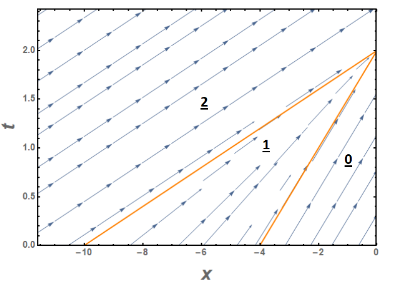
Figure 1: Regions of the $(t,{\bf x})$ space, where $T=2$ is the time when the seminar effectively begins, and their associated optimal drift $a(t,{\bf x})$. In regions (0) and (2) the drift stays constant and is denoted respectively $a^{(0)}$ and $a^{(2)}$ (here 5 and 2). In region (1),the drift is linear in x.

The (admittedly limited) goal of this paper will therefore be to analyse the Fokker-Planck equation for this velocity field in the small $\sigma$ regime, and to show that we can provide a very precise solution of this problem based just on the “classical trajectories” for a dynamics closely related to (but slightly different from) the $\sigma=0$ limit of Eq. (1).

The fact that this can be achieved for the Fokker-Planck equation can be seen readily by multiplying Eq. (1) by $\sigma^{2}$, and noting that it then has the structure of what Maslov Maslov and Fedoriuk (1981) has termed a “$\lambda$-pseudo differential operator”, in the sense that each partial derivative is associated with a factor $\lambda^{-1}\equiv\sigma^{2}$. This implies that a “semiclassical approximation” scheme can be applied to this equation in small $\sigma^{2}$ limit. This fact has of course been recognized for many years, and led to some publications Risken (1996); Shizgal and Nishigori (1990); Derevyanko et al. (2005). Most of them, however, use a rather indirect approach, making use of transformation of variable to a form more directly related to the Schrödinger equation and through a normal mode decomposition (cf eg Caroli et al. (1979) on the example of a diffusion in bistable potentials). We follow however here the philosophy of the ray method introduced in Cohen and Lewis (1967).

Our goal will thus be to to show that a direct approach where the time-dependent WKB approximation is applied directly on Eq. (1) can be used effectively to obtain a extremelly good approximation for the solution of the Fokker-Planck equation Eq. (1) with the drift field (3). We address thus here only the first (and simplest) step of the analysis of the coupled MFG equations system, and furthermore do this on a specific illustrative case. This gives us however the opportunity to discuss the application of the WKB approach in the perspective developed by Maslov Maslov and Fedoriuk (1981), in a way which is maybe a bit more transparent that what can be found in the literature Cohen and Lewis (1967), and leads in our view to a rather intuitive interpretation.

The paper will be organised as follows. In section II, we will give without justification the recipe for the construction of the WKB approximation. For the sake of clarity this will be done for a one dimensional problem, and we will assume that the initial density $m_{0}(x)$ is a gaussian. Section III will then provide a derivation of these WKB expressions, together with a generalization to higher dimensionality and to a larger class of initial densities. Readers with little interest in these formal issues may skip that section and go directly to section IV where the WKB approximation is applied to two simple examples where it turns out to provide the exact solution, as well as to the case corresponding to the drift field Eq. (3). Finally, we conclude in section V, and, for self-containedness, briefly sketch two rather standard derivations in appendices A and B.

II WKB approximation of a 1d Fokker-Planck equation

In this section, we provide, without any demonstration, the prescription for the construction of the WKB solution of the Fokker-Planck equation Eq. (1) in the small $\sigma$ regime. We limit ourselves here to the one-dimensional case and to gaussian initial densities

$$m_{0}(x)=\mathcal{N}\exp\left[-\frac{\mu(x-\bar{x}_{0})^{2}}{2\sigma^{2}}\right]\;,$$ (4)

where $\bar{x}_{0}$ is the center of the gaussian and $\mathcal{N}=\sqrt{\frac{\mu}{2\pi\sigma^{2}}}$ is a normalisation factor. More general $m_{0}(x)$ could easily be considered (see section III), but gaussians have an intrinsic interest, and, in addition, this also allows us to get the Green’s function of the equation by reducing the width of the gaussian to zero.

The semiclassical scheme follows three steps. The first one consists in constructing a Lagrangian symplectic manifold on which we can define an action. The second step uses this input to build the WKB approximation. Finally, we address how absorbing boundary conditions can be implemented in the semiclassical scheme.

II.1 Symplectic manifold and classical action

The Fokker-Planck equation (1) can be written as $\hat{L}m=0$ where we have introduced the $\lambda$-pseudo differential operator $\hat{L}\equiv[\lambda^{-1}\partial_{t}\cdot+\lambda^{-1}\partial_{x}(a\cdot)-\frac{1}{2}(\lambda^{-1}\partial_{x})^{2}\cdot]$ (with again $\lambda\equiv\sigma^{-2}$ assumed large). Using the usual mapping $\lambda^{-1}\partial_{x}\to p$, $\lambda^{-1}\partial_{t}\to E$, $\hat{L}$ can be associated with the classical symbol

$$L(x,t;p,E)=E+pa(x,t)-p^{2}/2\;,$$ (5)

which, if understood as a classical Hamiltonian leads to the canonical equations

$$\left\{\begin{aligned} &\dot{t}=\partial_{E}L=1\qquad&\dot{E}=-\partial_{t}L=-p\partial_{t}a\\ &\dot{x}=\partial_{p}L=a(t,x)-p\qquad&\dot{p}=-\partial_{x}L=-p\partial_{x}a\end{aligned}\right.\;.$$ (6)

Now, consider the initial gaussian distribution Eq. (4) for $\bar{x}_{0}$ and $\mu$ given. It can be written in the semiclassical form $m_{0}(x_{0})=\mathcal{N}\exp\left[\lambda S_{0}(x_{0})\right]$ with

$$S_{0}(x_{0})\equiv-\mu\frac{(x_{0}-\bar{x}_{0})^{2}}{2}\;.$$ (7)

At any point of space $x_{0}$, one can therefore initiate a classical trajectory at $t=t_{0}$ with an inital momentum

$$p_{0}(x_{0})=\nabla S_{0}(x_{0})=-\mu(x_{0}-\bar{x}_{0})\;,$$ (8)

and fulfilling the “compatibility condition”

$$L(x,t;p,E)\equiv 0\;.$$ (9)

The reunion of all these trajectories obtained from these intial conditions and the canonical equations (6) form a 2-dimensional manifold $\mathcal{M}=\{(t,\mathcal{x}(t,x_{0}),\mathcal{E}(t,x_{0})\mathcal{p}(t,x_{0})\}$ where $\mathcal{p}$, $\mathcal{x}$ and $\mathcal{E}$ respectively represent the value taken by $p$, $x$ and $E$ after evolving on this manifold from ${\bf r}_{0}=(t_{0},x_{0};E_{0}(x_{0}),p_{0}(x_{0}))$ for a time $t-t_{0}$.

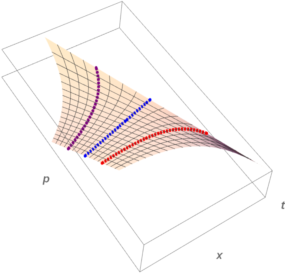
Figure 2: A typical manifold generated by the classical trajectories in region (1) of the drift field. In this case $a=\frac{x}{t-T}$, $\mu=1.5$, $\sigma=0.4$, $T=2$ and $\bar{x}_{0}=-5$. The dashed curves represent specific trajectories beginning at $x_{0}=-5.5$, $-5$ and $-4.5$ from left to right.

To the manifold $\mathcal{M}$, we can now associate a classical action

$$S(t,x)\equiv\int_{[\mathcal{L}:\bar{\bf r}_{0}\to{\bf r}]\subset\mathcal{M}}pdx+Edt\;$$ (10)

where $\bar{\bf r}_{0}=(t_{0},\bar{x}_{0};E\!=\!0,p\!=\!0)$ is the point on $\mathcal{M}$ above $\bar{\bf X}_{0}=(t_{0},\bar{x}_{0})$, and ${\bf r}\in\mathcal{M}$ is the point above ${\bf X}=(t,x)$.

We stress that, since $\mathcal{M}$ is a Lagrangian manifold, the integral in Eq. (10) can be taken on any path on $\mathcal{M}$ joining $\bar{\bf r}_{0}$ to ${\bf r}$. For instance, the action $S(t,x)$ can be computed either as

$$S_{1}(t,x)=\underbrace{\int_{\bar{x}_{0}}^{x_{0}(t,x)}p_{0}(x^{\prime})dx^{\prime}}_{S_{0}(x_{0})}+\int_{t_{0}}^{t}(\mathcal{p}(s,x_{0})\dot{\mathcal{x}}(s,x_{0})+\mathcal{E}(s,x_{0}))ds\;,$$

in which $x_{0}(t,x)$ is the initial position of the trajectory arriving at $x$ at time $t$, or as

$$S_{2}(t,x)=\int_{t_{0}}^{t}(\mathcal{p}(s,\bar{x}_{0})\dot{\mathcal{x}}(s,\bar{x}_{0})+\mathcal{E}(s,\bar{x}_{0}))ds+\int_{\mathcal{x}(t,\bar{x}_{0})}^{x}p(x^{\prime},t)dx^{\prime}\;,$$

with $p(x,t)$ the momentum coordinate of the point of $\mathcal{M}$ above $(t,x)$. Both expressions lead to the same result (i.e. $S_{1}(t,x)=S_{2}(t,x)=S(t,x)$). This is illustrated on Fig. 3.

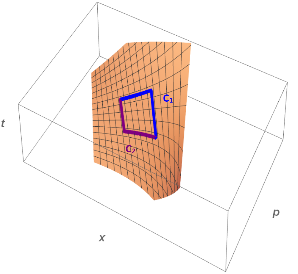
Figure 3: Same manifold as in Figure 2 where are highlighted two paths with same beginning and end. Because of the Langrangian nature of the manifold we can write $\int_{C_{1}}(E\dot{t}+p\dot{x})dt=\int_{C_{2}}(E\dot{t}+p\dot{x})dt$.

For the gaussian initial density we consider, the definition of the initial momentum given by (8) and the compatibility conditions $L\equiv 0$ impose that $\mathcal{p}(t,\bar{x}_{0})=0$ and $\mathcal{E}(t,\bar{x}_{0})=0$ for all time, yielding

$$S(t,x)=S_{2}(t,x)=\int^{x}_{\mathcal{x}(t,\bar{x}_{0})}p(t,x^{\prime})dx^{\prime}\;,$$ (11)

where the path of integration on the manifold is taken at constant time $t$ from the point above $\bar{x}\equiv\mathcal{x}(t,\bar{x}_{0})$ (evolution of the center of the distribution $\bar{x}_{0}$) to the point above $x$.

As a final comment, it is worth mentionning that, for more general initial conditions, $S_{0}(\bar{x}_{0})$ can be non-zero and should be added to the right-hand side of (10).

II.2 Semiclassical approximation for $m(t,x)$

With this definition of the action, the WKB approximation for the density of probability is expressed as

$$m_{\rm s.c.}(t,x)=\frac{\mathcal{N}}{\sqrt{\partial_{x_{0}}\mathcal{x}(t,x_{0})}}\exp\left[\lambda S(t,x)-\frac{1}{2}\int^{t}_{0}(\partial_{x}a)d\tau\right]\;,$$ (12)

where in the prefactor, $\mathcal{x}(t,x_{0})$ is the position of a trajectory started at $x_{0}$ at time $t\!=\!t_{0}$ (with thus a momentum $p_{0}(x_{0})$ given by Eq. (8)), and the integral in the exponential is taken along this trajectory. Except for the fact that the exponent is real rather than complex, the only difference with respect to the traditional WKB expressions derived in optics or in the context of the Schrödinger equation is the extra term $\frac{1}{2}\int^{t}_{0}(\partial_{x}a)d\tau$ in the exponent, which can be tracked back to the non-symmetric ordering of the operators $\hat{p}\equiv\lambda^{-1}\partial_{x}$ and $\hat{x}\equiv\times x$ in the Fokker-Planck equation.

II.3 Absorbing boundary conditions

We shall illustrate below this WKB approach with the problem corresponding to the drift velocity field Eq. (3), problem for which we assume an absorbing boundary condition at $x=0$. As such absorbing boundary conditions are rather common, we discuss now how to implement them in our semiclassical scheme.

Let us consider the semiclassical solution of the free problem (ie without the boundary condition)

$$m_{\rm free}(t,x)=\frac{\mathcal{N}}{\sqrt{\partial_{x_{0}}\mathcal{x}(t,x_{0})}}\exp\left[\lambda S(t,x)-\frac{1}{2}\int^{t}_{0}(\partial_{x}a)d\tau\right]\;.$$ (13)

For sake of simplicity, we assume that (as will be the case in the examples we are going to consider), the trajectories on which $S(t,x)$ is constructed are reaching $x=0$ with positive velocity.

Consider now the compatibility condition Eq. (9) at $x=0$, for an arbitrary time $t$, and with the choice $E=\partial_{t}S$

$$L(0,t;p,\partial_{t}S)=0\;.$$

It admits two solutions

$$\dot{x}=a(x,t)-p=\pm\sqrt{a^{2}+2\partial_{t}S}\;.$$ (14)

The one corresponding to a positive velocity is just $p_{+}(t)=\partial_{x}S(t,x\!=\!0)$. We can however generate another set of trajectories initiated at time $t$ at $x=0$ with momentum $p_{-}(t)=a+\sqrt{a^{2}(t,0)+2\partial_{t}S(t,0)}$ and energy $E(t)=\partial_{t}S(t,0)$. These trajectories have negative velocities and thus “bounce” off the boundary point $x=0$.

A “reflected” density

$$m_{\rm ref}(t,x)=\frac{\mathcal{N}}{\sqrt{\partial_{x_{0}}\tilde{\mathcal{x}}(t,x_{0})}}\exp\left[\lambda\tilde{S}(t,x)-\frac{1}{2}\int^{t}_{0}(\partial_{x}a)d\tau\right]\;,$$ (15)

can therefore be constructed in exactly the same way as before using the reflected trajectories $\tilde{\mathcal{x}}$ and reflected action $\tilde{S}$. At $x=0$, $m_{\rm ref}(t,0)=m_{\rm free}(t,0)$ since $\partial_{t}S(t,0)=\partial_{t}\tilde{S}(t,0)=E(t,0)$ is the same for both (and thus one should just impose $S(t_{0},0)=\tilde{S}(t_{0},0)$ for an arbitrary time $t_{0}$), and $\partial_{x_{0}}\tilde{\mathcal{x}}(t,x_{0})=\partial_{x_{0}}\mathcal{x}(t,x_{0})$ since at $x=0$ only the momentum has changed but not the position. Therefore, the total density

$$m_{\rm tot}(t,x)=m_{\rm free}(t,x)-m_{\rm ref}(t,x)$$ (16)

is a semicalssical solution to the Fokker-Planck equation (1) which fulfills the absorbing boundary condition $m_{\rm tot}(t,0)=0$.

III Derivation and generalisation

We provide now a derivation (and some generalisation) of Eq. (12). Our approach is very similar in spirit to the “ray method” developed by Cohen and Lewis Cohen and Lewis (1967), but follow more closely the WKB formalism developped by Maslov Maslov and Fedoriuk (1981), that we feel might be easier to access for physicists.

We therefore want to describe the evolution of an initial density (at $t=t_{0}$) which is in the “semiclassical form”

$$m_{0}({\bf x})=\phi_{0}({\bf x})\exp\left[\lambda S_{0}({\bf x})\right]\;,$$ (17)

with $\bf x\in\mathbb{R}^{d}$. Such form includes Gaussian densities such as Eq. (4), but are significantly more general.

By writing $(\sigma^{-2}\equiv\lambda)$, the Fokker-Planck equation reads in the more general case,

$$0=\lambda^{-1}\partial_{t}m+\lambda^{-1}\nabla({\bf a}(t,{\bf x})m)-\frac{1}{2}\lambda^{-2}\Delta m=\hat{L}m\;,$$ (18)

which up to the $i$ factors, looks very much like a $\lambda$-pseudo differential Maslov operator of symbol

$$L({\bf x},t;{\bf p},E)=E+{\bf a}({\bf x},t)\!\cdot\!{\bf p}-{\bf p}^{2}/2\;.$$ (19)

Following Maslov’s derivation Maslov and Fedoriuk (1981), let us consider the ansatz

$$m(t,{\bf x})=\phi(t,{\bf x})\exp\left[\lambda S(t,{\bf x})\right]\;,$$ (20)

with $\phi(t_{0},{\bf x})=\phi_{0}({\bf x})$ and $S(t_{0},{\bf x})=S_{0}({\bf x})$.

Writing ${\bf X}\equiv(t,{\bf x})$, ${\bf P}\equiv(E,{\bf p})$, Eq. (18) becomes

$$\hat{L}\left[\phi({\bf X})e^{\lambda S({\bf X})}\right]=0=e^{\lambda S({\bf X})}\left[R_{0}\phi({\bf X})+\lambda^{-1}R_{1}\phi({\bf X})+O(\lambda^{-2})\right]$$ (21)

with

$$R_{0}=L({\bf X};\partial_{{\bf X}}S)\;,$$ (22)

$$R_{1}=\langle\partial_{{\bf P}}L({\bf X};\partial_{{\bf X}}S),\partial_{{\bf X}}\phi\rangle+\frac{1}{2}\left\{{\rm Tr}\left[\partial^{2}_{{\bf P}{\bf P}}L({\bf X};\partial_{{\bf X}}S)\partial^{2}_{{\bf X}{\bf X}}S\right]+{\rm Tr}\left[\partial^{2}_{{\bf X}{\bf P}}L({\bf X};\partial_{{\bf X}}S)\right]\right\}\phi\;.$$ (23)

Neglecting terms of order $\lambda^{-2}$ and higher, solving Eq. (18) amounts to solving $R_{0}=0$ and $R_{1}=0$.

III.1 $R_{0}=0$, Hamilton-Jacobi equation

The equation $(R_{0}=0)$ can be rewritten as an Hamilton-Jacobi equation on $S$

$$L({\bf X};\partial_{{\bf X}}S)=\partial_{t}S+{\bf a}(t,{\bf x})\!\cdot\!{\bf\nabla}S-\frac{1}{2}(\nabla S)^{2}=0\;,$$ (24)

with an initial condition at $t=t_{0}$

$$S(t_{0},{\bf x}_{0})=S_{0}({\bf x}_{0})\;.$$ (25)

Solution of this kind of equations is typically obtained through the method of characteristics. Here this amounts to build a one paramater family of rays $(t,{\bf x};E,{\bf p})_{{\bf x}_{0}}(s)\equiv{\bf r}(s,{\bf x}_{0})$, indexed by ${\bf x}_{0}$, which follow – for a fictitious time $s$ – the Hamilton dynamics associated with $L$:

$$\left\{\begin{aligned} &\dot{t}=\partial_{E}L=1\qquad&\dot{E}=\partial_{t}L=-{\bf p}\!\cdot\!\partial_{t}{\bf a}\ \ \ \\ &\dot{\bf x}=\partial_{\bf p}L={\bf a}(t,{\bf x})-{\bf p}\qquad&\dot{\bf p}=-\partial_{\bf x}L=-{\bf p}\!\cdot\!\partial_{\bf x}{\bf a}\\ \end{aligned}\right.\;,$$ (26)

with initial the conditions

$$\left\{\begin{aligned} &{\bf r}(0,{\bf x}_{0})=(E_{0},t_{0},{\bf p}_{0}({\bf x}_{0}),{\bf x}_{0})\\ &L({\bf r}(0,{\bf x}_{0}))=0\\ \end{aligned}\right.\;$$ (27)

corresponding to

$${\bf p}_{0}({\bf x}_{0})=\partial_{{\bf x}_{0}}S_{0}({\bf x}_{0})\;.$$ (28)

Eq. (27) fixes $E_{0}$ and it is clear from Eqs. (26) that we can take $s\equiv t-t_{0}$.

As stressed in the previous section, the family of rays defined by Eqs. (26)-(27) form a Lagrangian manifold, thus, according to the method of characteristics (cf appendix A), the solution of Eq. (24) reads

$$S(t,{\bf x})=\int_{\bar{\bf X}_{0}}^{{\bf X}}Edt+{\bf p}\!\cdot\!d{\bf x}\;,$$ (29)

where the integral is taken on any path on the manifold starting above the point $\bar{\bf X}_{0}=(t_{0},\bar{\bf x}_{0})$ such that $S_{0}(\bar{\bf x}_{0})=0$ and ending on the point above ${\bf X}=(t,{\bf x})$.

III.2 $R_{1}=0$, transport equation

We begin by focusing on the first term of $R_{1}$ that we rewrite more explicitly using the canonical Hamilton-Jacobi equations

$$\langle\partial_{{\bf P}}L({\bf X},\partial_{{\bf X}}S),\partial_{{\bf X}}\phi\rangle=\partial_{t}\phi+(\textbf{a}(t,{\bf x})-\partial_{{\bf x}}S)\partial_{{\bf x}}\phi=\partial_{t}\phi+\dot{{\bf x}}\partial_{{\bf x}}\phi=\frac{D\phi}{Dt}\;,$$ (30)

where $\frac{D}{Dt}$ represents the time derivative along the flow. This allows us to write the equation $(R_{1}=0)$ as a simple evolution equation

$$\frac{D\phi}{Dt}=-\left\{\frac{1}{2}{\rm Tr}\left[\partial^{2}_{{\bf P}{\bf P}}L({\bf X},\partial_{{\bf X}}S)\partial^{2}_{{\bf X}{\bf X}}S\right]+{\rm Tr}\left[\partial^{2}_{{\bf X}{\bf P}}L\right]\right\}\phi\;.$$ (31)

To solve this equation we will make use of Liouville’s formula, which states that for a dynamical system

$$\frac{d{\bf x}}{dt}=f({\bf x})\;,$$ (32)

and for any $(d\!-\!1)$-parameter family of trajectories ${\bf x}(t,\bm{\alpha})$ indexed by $\bm{\alpha}\in\mathbb{R}^{(d-1)}$, the determinant $J(t,\bm{\alpha})\equiv\det\biggl{[}\frac{\partial{\bf x}(t,\bm{\alpha})}{\partial(t,\bm{\alpha})}\biggr{]}$ fulfills

$$\frac{D\ln J}{Dt}={\rm Tr}\biggl{[}\frac{df}{d{\bf x}}({\bf x}(t,\bm{\alpha}))\biggr{]}\;.$$ (33)

(Elements of a demonstration are given in appendix B for the sake of completeness.) Using the canonical equations we have

$$\dot{{\bf X}}=\partial_{{\bf P}}L\;.$$ (34)

Noting that we can write ${\bf X}\equiv(t,\bm{\mathcal{x}}(t,{\bf x}_{0}))$ and having $J$ denote $\det[\partial_{t,{\bf x}_{0}}{\bf X}]$, Liouville’s formula reads

$$\frac{D\ln(J)}{Dt}={\rm Tr}\bigl{[}\partial_{\bf X}(\partial_{\bf P}L)\bigr{]}={\rm Tr}[\partial^{2}_{{\bf P}{\bf X}}L+\partial^{2}_{{\bf P}{\bf P}}L\partial^{2}_{{\bf X}{\bf X}}S]\;.$$ (35)

Hence Eq. (31) becomes

$$\frac{D\phi}{Dt}+\frac{1}{2}\frac{D}{Dt}(\ln J)\phi=-\frac{1}{2}{\rm Tr}[\partial^{2}_{{\bf X}{\bf P}}L]\phi\;,$$ (36)

and, multiplying both sides by $\sqrt{J}$,

$$\frac{D}{Dt}\bigl{[}\sqrt{J}\phi\bigr{]}=-\frac{1}{2}{\rm Tr}\left[\partial^{2}_{{\bf X}{\bf P}}L\right]\sqrt{J}\phi\;.$$ (37)

Finally, we have

$$\phi({\bf x}(t,{\bf x}_{0}))=\frac{\sqrt{J({\bf x}(t_{0},{\bf x}_{0}))}}{\sqrt{J({\bf x}(t,{\bf x}_{0}))}}\phi({\bf x}(t_{0},{\bf x}_{0}))\exp\biggl{(}-\frac{1}{2}\int^{t}_{t_{0}}{\rm Tr}\left[\partial^{2}_{{\bf X}{\bf P}}L\right]d\tau\biggr{)}$$ (38)

where $\sqrt{J({\bf x}(t_{0},{\bf x}_{0})})=1$ and, for $L$ given by Eq. (19), ${\rm Tr}[\partial^{2}_{{\bf X}{\bf P}}]={\rm div}\,{\bf a}$. In 1d $J$ would simply become $\partial_{x_{0}}\mathcal{x}$, yielding the prefactor in Eq. (12).

It is also worth noting that Eq. (31) can be solved in multiple ways, another possibility would be

$$\frac{D}{Dt}\bigl{[}J\phi\bigr{]}=+\frac{1}{2}{\rm Tr}\left[\left(\partial^{2}_{{\bf P}^{2}}L\right)\cdot\left(\partial^{2}_{{\bf X}^{2}}S\right)\right]J\phi\;,$$ (39)

implying

$$\phi({\bf x}(t,{\bf x}_{0}))=\frac{J({\bf x}(t_{0},{\bf x}_{0}))}{J({\bf x}(t,{\bf x}_{0}))}\phi({\bf x}(t_{0},{\bf x}_{0}))\exp\biggl{(}+\frac{1}{2}\int^{t}_{t_{0}}{\rm Tr}\left[\left(\partial^{2}_{{\bf P}^{2}}L\right)\cdot\left(\partial^{2}_{{\bf X}^{2}}S\right)\right]d\tau\biggr{)}\;.$$ (40)

Here $J$ serves only as a prefactor; it has no particular physical meaning, and either expressions cand be used.

IV Application to the seminar problem

For a 1d problem, and writing $\lambda^{-1}\equiv\sigma^{2}$, the semiclassical expression for $m$ reads

$$m(t,x)=\frac{\mathcal{N}}{\sqrt{\partial_{x_{0}}\mathcal{x}}}\exp\left[\frac{S(t,x)}{\sigma^{2}}-\frac{1}{2}\int^{t}_{0}(\partial_{x}a)d\tau\right]\;.$$ (41)

We will use this expression to study the different drift regimes (cf Eq. (3)) presented by the seminar problem for gaussian initial condition at $t\!=\!0$

$$m_{0}(x)=\mathcal{N}\exp\bigg{[}-\frac{\mu(x_{0}-\bar{x}_{0})^{2}}{2\sigma^{2}}\biggr{]}=\mathcal{N}\exp\bigg{[}\frac{S_{0}(x_{0})}{\sigma^{2}}\biggr{]}\;,$$ (42)

to which through Eq. (8) we associate the one-parameter family of intial points in phase space

$${\bf r}(x_{0})=(t\!=\!0,x_{0},E_{0}(x_{0}),p_{0}(x_{0}))$$ (43)

corresponding to

$$p_{0}(x_{0}) =\partial_{x_{0}}S_{0}(x_{0})=-\mu(x_{0}-\bar{x}_{0})\;,$$

$$E_{0}(x_{0}) =\frac{p^{2}_{0}(x_{0})}{2}-p_{0}(x_{0})a(x_{0},t\!=\!0)\;.$$

IV.1 Constant drift

Let us start with the simple case of a constant drift $a$ (this would correspond to regions (0) or (2) in Fig. 1). In order to obtain the density as expressed in Eq. (41) there are two terms we first need to compute, the prefactor $\partial_{x_{0}}\mathcal{x}(t,x_{0})$ and the action $S(t,x)$. To do so we start from the canonical equation of motion

$$\left\{\begin{aligned} &\dot{p}=-\partial_{x}L=-p\partial_{x}a=0\\ &\dot{x}=\partial_{p}L=a-p\mbox{ ( = const. along a trajectory) . }\end{aligned}\right.$$ (44)

For the one-parameter family of trajectories Eq. (43), this leads to

$$\left\{\begin{aligned} &\mathcal{p}(t,x_{0})=\mu(\bar{x}_{0}-x_{0})\\ &\mathcal{x}(t,x_{0})=x_{0}+[a-\mathcal{p}(t,x_{0})]t=x_{0}(1+t\mu)+t(a-\mu\bar{x}_{0})\;.\end{aligned}\right.$$ (45)

The prefactor is then readily obtained as

$$\partial_{x_{0}}\mathcal{x}(t,x_{0})=1+t\mu\;.$$ (46)

The action is computed noticing that, along the “center of mass” trajectory $\mathcal{x}(t,\bar{x}_{0})$, the momentum $\mathcal{p}(t,\bar{x}_{0})$ and energy $\mathcal{E}(t,\bar{x}_{0})$ remain identically zero. Hence, $\mathcal{M}=\{(t,\mathcal{x}(t,x_{0}),\mathcal{E}(t,x_{0})\mathcal{p}(t,x_{0})\}$ being Lagrangian,

$$S(t,x)=\int^{x}_{\mathcal{x}(t,\bar{x}_{0})}p(t,x^{\prime})dx^{\prime}\;,$$ (47)

$p(t,x)$ being the momentum of the point above $(x,t)$ on $\mathcal{M}$. Noting $x_{0}(t,x)$ the initial position of a trajectory arriving at $x$ at time $t$ (i.e. such that $x=\mathcal{x}(t,x_{0}))$, the second equation of (45) gives

$$x_{0}(t,x)=\frac{x-at+\mu\bar{x}_{0}t}{1+\mu t}\;,$$ (48)

and the first one

$$p(t,x)=-\frac{\mu}{1+\mu t}\left(x-(\bar{x}_{0}+at)\right)\;.$$ (49)

After integration, this last expression yields,

$$S(t,x)=-\biggl{(}\frac{\mu t}{1+\mu t}\biggr{)}\biggl{(}\frac{(x-\bar{x}_{0}-at)^{2}}{2t}\biggr{)}\ .$$ (50)

Finally, using Eq. (41) we have

$$m(t,x)=\sqrt{\frac{\mu}{2\pi\sigma^{2}}}\frac{1}{\sqrt{1+t\mu}}\exp\biggl{[}-\biggl{(}\frac{\mu t}{1+\mu t}\biggr{)}\biggl{(}\frac{(x-\bar{x}_{0}-at)^{2}}{2t\sigma^{2}}\biggr{)}\biggr{]}\;,$$ (51)

which turns out to be the exact expression for the evolution of a initial Gaussian density in the case of a constant drift. This is actually expected since going back to the derivation of the semiclassical approximation, we see that the terms neglected contain only second (or higher) order spatial derivative of $a$ which are identically zero in the case of a constant drift.

If $\mu\rightarrow\infty$, $m(0,x)\rightarrow\delta(x-\bar{x}_{0})$, and

$$m(t,x)\rightarrow G(t,x,\bar{x}_{0})=\sqrt{\frac{1}{2\pi t\sigma^{2}}}\exp\biggl{[}-\frac{(x-\bar{x}_{0}-at)^{2}}{2t\sigma^{2}}\biggr{]}\;,$$ (52)

which indeed is the exact Green function of the Fokker-Planck equation for a constant drift.

Absorbing boundary condition at $x=0$

To implement the absorbing boundary condition at $x=0$, we follow the procedure discussed earlier in section II.3 and construct the “reflected” action

$$\tilde{S}(t,x)=S(t,0)+\int_{0}^{x}p_{-}(t,x^{\prime})dx^{\prime}\;,$$ (53)

where $p_{-}(t,x)$ is the reflected momentum.

To compute this quantity, let us note

$$t_{\rm abs}=\frac{x_{0}}{\mu(\bar{x}_{0}-x_{0})-a}$$

the time at which the trajectory initiated at $x_{0}$ reaches 0 (and is thus “absorbed”). Since velocity is constant on a given trajectory, we can express the velocity before the bounce as $\dot{x}_{+}(x_{0})=-x_{0}/t_{\rm abs}$ and thus just after the bounce as $\dot{x}_{-}(x_{0})=+x_{0}/t_{\rm abs}$. Eqs. (44) then give

$$\mathcal{p}_{-}(t>t_{\rm abs},x_{0}) =a-\frac{x_{0}}{t_{\rm abs}}=2a-\mu(\bar{x}_{0}-x_{0})\;,$$ (54)

$$\mathcal{x}(t>t_{\rm abs},x_{0}) =\frac{x_{0}}{t_{\rm abs}}(t-t_{\rm abs})=-x_{0}(1+\mu t)-at+\mu\bar{x}_{0}t\;.$$ (55)

Defining $\tilde{x}_{0}(t,x)$ the initial position of a trajectory arriving at $\mathcal{x}(t,x_{0})=x$ after reflection at $x=0$, we thus have from Eq. (55)

$$\tilde{x}_{0}(t,x)=\frac{\mu t\bar{x}_{0}-at-x}{1+\mu t}\;,$$ (56)

which inserted into Eq. (54) gives

$$p_{-}(t,x)=2a-\biggl{(}\frac{\mu t}{1+\mu t}\biggr{)}\biggl{(}\frac{x+\bar{x}_{0}+at}{t}\biggr{)}\;.$$ (57)

Performing the integral in Eq. (53), and noting that the lower bound cancels the term $S(t,x\!=\!0)$, we thus have

$$\tilde{S}(t,x)=2ax-\biggl{(}\frac{\mu t}{1+\mu t}\biggr{)}\biggl{(}\frac{(x+\bar{x}_{0}+at)^{2}}{2t}\biggr{)}\;,$$ (58)

giving for the total (incident plus reflected) density

$$\begin{aligned} m_{\rm tot}(t,x)=\sqrt{\frac{\mu}{2\pi\sigma^{2}}}\frac{1}{\sqrt{1+t\mu}}&\biggl{\{}\exp\biggl{[}-\biggl{(}\frac{\mu t}{1+\mu t}\biggr{)}\biggl{(}\frac{(x-\bar{x}_{0}-at)^{2}}{2t\sigma^{2}}\biggr{)}\biggr{]}\\ &-\exp\biggl{(}\frac{2ax}{\sigma^{2}}\biggr{)}\exp\biggl{[}-\biggl{(}\frac{\mu t}{1+\mu t}\biggr{)}\biggl{(}\frac{(x+\bar{x}_{0}+at)^{2}}{2t\sigma^{2}}\biggr{)}\biggr{]}\biggr{\}}\end{aligned}\;.$$ (59)

This fulfils the absorbing boundary conditions $m_{\rm tot}(t,0)=0$ and, for the same reason as above, is an exact expression, thus yielding the exact Green function of the Fokker-Planck equation as $\mu\rightarrow\infty$.

IV.2 Linear drift

We will now consider a linear drift $a(x,t)={x}/{(t-T)}$, with $T>t$ the time at which the seminar begins, associated with region (1) in Fig. 1. The canonical equations become

$$\left\{\begin{aligned} &\dot{x}=\partial_{p}L=a-p=\frac{x}{t-T}-p\\ &\dot{p}=-\partial_{x}L=-p\partial_{x}a=-\frac{p}{t-T}\;,\end{aligned}\right.$$ (60)

giving

$$\left\{\begin{aligned} &\mathcal{p}(t,x_{0})=p_{0}(x_{0})\frac{T}{T-t}=\frac{\mu T(\bar{x}_{0}-x_{0})}{T-t}\\ &\mathcal{x}(t,x_{0})=\frac{x_{0}(T-t)}{T}-\mu t(\bar{x}_{0}-x_{0})\;.\end{aligned}\right.$$ (61)

We thus have $\partial\mathcal{x}/\partial x_{0}=(T-t+\mu tT)/T$, which together with $\int_{0}^{t}(\partial_{x}a)d\tau=\log[(T-t)/T]$ yieds for the prefactor to

$$\frac{\mathcal{N}}{\sqrt{\partial_{x_{0}}\mathcal{x}}}\exp\left[-\frac{1}{2}\int^{t}_{0}(\partial_{x}a)d\tau\right]=\sqrt{\frac{\mu}{2\pi\sigma^{2}}}\sqrt{\frac{T^{2}}{(\mu tT+T-t)(T-t)}}\;.$$ (62)

Turning now to the action, we have from the second equation of (61),

$$x_{0}(t,x)=(x-\mu t\bar{x}_{0})\frac{T}{T-t+\mu Tt}\;,$$ (63)

which, inserted into the first equation of (61) gives for the momentum $p(t,x)$,

$$p(t,x)=\frac{\mu\,T\,(\bar{x}_{0}(T-t)-Tx)}{(T-t)(T-t+\mu Tt)}\;,$$ (64)

leading by integration to

$$S(t,x)=\int^{x}_{\mathcal{x}(t,\bar{x}_{0})}p(t,x^{\prime})dx^{\prime}=\frac{\mu(\bar{x}_{0}(t-T)-Tx)^{2}}{2(T-t)(T-t+\mu Tt)}\;.$$ (65)

Using Eq. (41), and computing the reflected action $\tilde{S}(t,x)$ following the same procedure as in Section IV.1, giving

$$\tilde{S}(t,x)=\frac{\mu(xT+(T-t)\bar{x}_{0})^{2}}{2(t-T)(T-t+\mu Tt)}\;,$$ (66)

we get for the evolution of a Gaussian initial density with a linear drift velocity and absorbing boundary conditions at $x\!=\!0$

$$m(t,x) =\sqrt{\frac{\mu}{2\pi\sigma^{2}}}\sqrt{\frac{T^{2}}{(\mu tT-T-t)(T-t)}}$$ (67)

$$\biggl{\{}\exp\biggl{[}\frac{\mu(xT-(T-t)\bar{x}_{0})^{2}}{2\sigma^{2}(t-T)(T-t+\mu Tt)}\biggr{]}-\exp\biggl{[}\frac{\mu(xT+(T-t)\bar{x}_{0})^{2}}{2\sigma^{2}(t-T)(T-t+\mu Tt)}\biggr{]}\biggr{\}}\;.$$

As $\mu\rightarrow\infty$ we recover the Green function of the correponding Fokker-Planck equation

$$G(t,x,\bar{x}_{0})=\sqrt{\frac{T}{2\pi\sigma^{2}t(T-t)}} \biggl{\{}\exp\biggl{(}-\frac{T(x-\frac{T-t}{T}\bar{x}_{0})^{2}}{2\sigma^{2}t(T-t)}\biggr{)}$$ (68)

$$-\exp\biggl{(}-\frac{T(x+\frac{T-t}{T}\bar{x}_{0})^{2}}{2\sigma^{2}t(T-t)}\biggr{)}\biggr{\}}\;.$$

Again, because the second $x$ derivative of the drift is zero, expressions (67) and (68) are exact.

IV.3 Coupling the two solutions

We now consider the full problem corresponding to the drift field Eq. (3), taking into account the possibility that agents begining in region (0) or (2) (associated with constant drifts $a^{(0)}$ and $a^{(2)}$) may leak into region (1) (associated with a linear drift $a(x,t)=x/(t-T)$), and reciprocally. We focus here on times $t\leq T$ and on the configuration where the agents start their diffusion in region (1), which is the one of interest from the point of view of mean field games. Corresponding expressions for a group of agents initially located in region (2) are given in appendix C.

We begin by defining $x^{*(n)}(x_{0})$, $p^{*(n)}(x_{0})$ and $t^{*(n)}(x_{0})$, ($n=0,2$), the position, impulsion and time at which a trajectory intiated at ${\bf r}(x_{0})$ (cf Eq. (43)) crosses the boundary between regions (1) and $(n)$. Using Eq. (61) together with the fact that the boundary is the $x=a^{(n)}(t-T)$ straight line, we may write

$$x^{*(n)}(x_{0})=a^{(n)}(t^{*(n)}-T)=x_{0}\frac{(T-t^{*(n)})}{T}-\mu(\bar{x}_{0}-x_{0})t^{*(n)}(x_{0})\;.$$ (69)

We then compute $t^{*(n)}$ by inverting this last equation and obtain $p^{*(n)}$ inserting this newly found $t^{*(n)}$ expression in Eq. (61)

$$\left\{\begin{aligned} &t^{*(n)}(x_{0})=T\biggl{[}1-\frac{\mu T(\bar{x}_{0}-x_{0})}{a^{(n)}T+x_{0}+\mu T(\bar{x}_{0}-x_{0})}\biggr{]}\\ &p^{*(n)}(x_{0})=\frac{a^{(n)}T+\mu T(\bar{x}_{0}-x_{0})+x_{0}}{T}\end{aligned}\right.\qquad.$$ (70)

Before the crossing ($t<t^{*(n)}$) the agents do not feel the effects of the drift change, and their trajectories remain the same as in Eq. (61). In region (1), ($x^{*(0)}<x<x^{*(2)}$), the prefactor is thus obtained as Eq. (62) and the action as Eq. (65). We will now focus on the expression of the density after the crossing, the complete solution being simply obtained by patching the linear and the leaking densities.

Using the canonical equations in the region in which the agents are leaking, we have for $t>t^{*(n)}$,

$$\left\{\begin{aligned} &\mathcal{x}^{(n)}(t,x_{0})=x^{*(n)}+(a^{(n)}-p^{*(n)})(t-t^{*(n)})=x_{0}\frac{T-t}{T}-t\mu(\bar{x}_{0}-x_{0})\\ &\mathcal{p}^{(n)}(t,x_{0})=p^{*(n)}\end{aligned}\right.\;\;.$$ (71)

Let $x_{0}(t,x)$ be the initial position of a trajectory arriving at $x$ at time $t$ (thus $\mathcal{x}_{n}(t,x_{0})=x$), $t^{*(n)}(t,x)$ the time at which this trajectory crosses the boundary between the two regions, and $p^{*(n)}(t,x)$ the momentum at the crossing

$$\left\{\begin{aligned} &x_{0}(t,x)=\frac{T(x-\mu t\bar{x}_{0})}{T-t-\mu Tt}\\ &t^{*(n)}(t,x)=T\biggl{\{}1-\frac{\mu T\bigl{[}\bar{x}_{0}-x_{0}(t,x)\bigr{]}}{aT+x_{0}(t,x)+\mu T(\bar{x}_{0}-x_{0}(t,x))}\biggr{\}}\\ &p^{*(n)}(t,x)=\frac{aT+\mu T\bigl{[}\bar{x}_{0}-x_{0}(t,x)\bigr{]}+x_{0}(t,x)}{T}\\ \end{aligned}\right.\;\;.$$ (72)

We may now compute the prefactor

$$\frac{\mathcal{N}}{\sqrt{\partial_{x_{0}}\mathcal{x}_{n}}} \exp\left[-\frac{1}{2}\int^{t^{*}(t,x)}_{0}(\partial_{x}a^{(1)})d\tau\right]=$$ (73)

$$\sqrt{\frac{\mu}{2\pi\sigma^{2}}\frac{T}{T-t+\mu Tt}\frac{\mu T(\bar{x}_{0}-x)+x+a^{(n)}(T-t+\mu Tt)}{\mu T(\bar{x}_{0}-x)-\mu t\bar{x}_{0}}}\;,$$

and the action

$$S^{(n)}_{\rm{leak}}(t,x)=\int^{a^{(n)}(t-T)}_{\bar{x}}p^{(1)}(t,x^{\prime})dx^{\prime}+\int^{x}_{a^{(n)}(t-T)}p^{*(n)}(t,x^{\prime})dx^{\prime}$$ (74)

$$=\frac{-(a^{(n)})^{2}(t-T)(T-t+\mu Tt)+2a^{(n)}(T-t+\mu Tt)x+(1-\mu T)x^{2}+2\mu Tx\bar{x}_{0}+\mu(t-T)\bar{x}_{0}^{2}}{2(T-t+\mu tT)}\;,$$

with $p^{(1)}$ given by Eq. (64). We note that if both $x$ and $\bar{x}_{0}$ belong to the boundary between region (1) and region (n), the prefactor diverges because of diffraction effects that should be treated specifically.

The reflected action is computed through the usual procedure, but, this time, taking into account that the reflected trajectory may also transit from a region to an other

$$\tilde{S}_{\rm{leak}}(t,x)= S^{(n)}_{\rm{leak}}(t,0)+\int_{0}^{\min[x;a^{(1)}(t-T)]}p^{*(0)}_{-}(t,x^{\prime})dx^{\prime}$$ (75)

$$+\int_{a^{(1)}(t-T)}^{\min\left[\max[x;a^{(1)}(t-T)];a^{(2)}(t-T)\right]}p^{(1)}_{-}(t,x^{\prime})dx^{\prime}$$

$$+\int_{a^{(2)}(t-T)}^{\max[x,a^{(2)}(t-T)]}p^{*(2)}_{-}(t,x^{\prime})dx^{\prime}\;,$$

with $p^{*(n)}_{-}$ the reflected leaking momentum in region (n) and $p^{(1)}_{-}$ the reflected linear drift momentum. Complete, explicit, expressions are given in appendix C (cf Eqs. (88), (89) and (90)). However the contribution of reflected trajectories decay exponentially away from the absorbing boundary $x=0$. Assuming $t\leq T$ as we do here, this implies that unless $t\approx T$, we can assume the contribution of reflected trajectories are important only when they are still in region (0), and the reflected action can be approximated as

$$\tilde{S}_{\rm{leak}}(t,x)=2a^{(0)}x-\frac{1}{2(T-t+\mu tT)} \biggl{[}-(a^{(0)})^{2}(t-T)(T-t+\mu Tt)+2a^{(0)}(T-t+\mu Tt)x$$ (76)

$$+(1-\mu T)x^{2}+2\mu Tx\bar{x}_{0}+\mu(t-T)\bar{x}_{0}^{2}\biggr{]}\;.$$

We can show that, for this specific drift field, the reflected prefactor is the same as the direct one. Eventually, using Eq.(41), we have

$$m_{\rm{leak}}(t,x)= \sqrt{\frac{\mu}{2\pi\sigma^{2}}\frac{T}{T-t+\mu Tt}\frac{\mu T(\bar{x}_{0}-x)+x+a^{(n)}(T-t+\mu Tt)}{\mu T(\bar{x}_{0}-x)-\mu t\bar{x}_{0}}}\biggl{\{}$$ (77)

$$\exp\biggl{(}\frac{S_{\rm{leak}}(t,x)}{\sigma^{2}}\biggr{)}-\exp\biggl{(}\frac{\tilde{S}_{\rm{leak}}(t,x)}{\sigma^{2}}\biggr{)}\biggr{\}}\;.$$

Contrarily to constant and linear drifts which represent non-generic cases for which the WKB expression is exact, the above result is an approximation valid only in the semiclassical regime of small $\sigma$’s. To be a bit more quantitative, we thus introduce the dimensionless parameter $K$ defined as the ratio between the drift time $\tau_{\rm{drift}}={\mathcal{x}(t,\bar{x}_{0})}/{a}$, the time needed to get from $x=\mathcal{x}(t,\bar{x}_{0})$ to the location of the absorbing boundary condition $x=0$ at speed $a$, and the diffusion time $\tau_{\rm{diffusion}}={\mathcal{x}^{2}(t,\bar{x}_{0})}/{\sigma^{2}}$, time it would take to a purely diffusive process to spread the density from its center in $x=\mathcal{x}(t,\bar{x}_{0})$ to $x=0$. Thus

$$K=\frac{\tau_{\rm{drift}}}{\tau_{\rm{diffusion}}}=\biggl{|}\frac{\sigma^{2}}{a\mathcal{x}(t,\bar{x}_{0})}\biggr{|}\propto\sigma^{2}\;.$$ (78)

The “small noise” [semiclassical] regime can be therefore characterized by $K\ll 1$, and the large noise regime by $K\gg 1$. Note that $K$ usually depends on time. Fig. 4 shows a comparison between a numerical solution and the semiclassical approximation for different small values of $K$, fixing $\sigma$ and varying $t$.

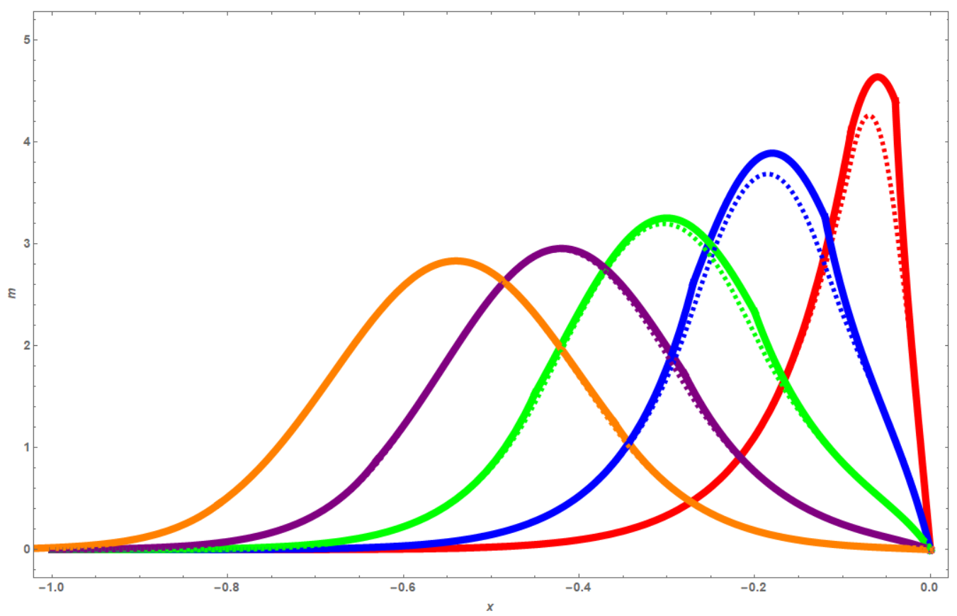
Figure 4: Spatial distribution of the agents, dashed lines show the numerical solution while solid lines show the approximation. From left to right, $K=0.19$, $K=0.24$, $K=0.33$, $K=0.56$, $K=1.67$. In this case $T=2$, $a^{(0)}=0.4$, $a^{(2)}=0.9$, $\sigma=0.2$, $\bar{x}_{0}=1.2$ and $\mu=10^{6}$.

As we can see the semiclassical approximation is almost indistinguishable from the numerical solution up to $K=0.33$ and remains good for $K$ slightly greater than one even if we can observe small discrepancies. Looking at larger values of $\sigma$ (and hence $K$), cf. Fig. 5, we see that even for the largest value of $K$ considered ($K=6.66$), the agreement is still rather good although the difference with the exact result becomes more significant.

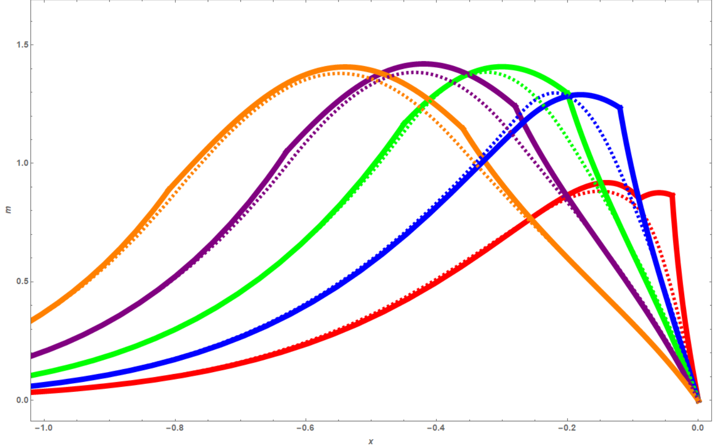
Figure 5: Spatial distribution of the agents, dashed lines show the numerical solution while solid lines show the approximation. From left to right, $K=0.74$, $K=0.95$, $K=1.33$, $K=2.22$, $K=6.66$. In this case $T=2$, $a^{(0)}=0.4$, $a^{(2)}=0.9$, $\sigma=0.4$, $\bar{x}_{0}=1.2$ and $\mu=10^{6}$.

The fact that the source of errors in the semiclassical treatment is generated only at the boundaries between the various regions explains the effectiveness of the approximation in this particular setup.

V Conclusion

In this paper we proposed a new take on the WKB approximation scheme to study the Fokker-Planck equation. This approach, based on Maslov’s geometric perspective, offers what we think to be a transparent way of tackling the Fokker-Planck equation, which we illustrated here on a problem motivated by a simple toy model of mean field games theory.

As stressed in the introduction, we have addressed here only a very small part of the program which would consist in providing a “ray theory” of mean field games in the small but non zero-noise limit. This program would involve a few steps (to start with a ray theory of the Hamilton-Jacobi-Bellman equation and then dealing with the coupling between the two) which are significantly more involved. We leave these for future research, but we are convinced that the WKB approach we propose provide a sound start for this program.

Appendix A Method of characteristics

The method of characteristics is typically used to solve first-order partial differential equations. It aims to reduce a PDE to a family of ODEs that can be easily integrated. A rather complete discussion of this method can be found for instance in chapter II of R. Courant (1962).

In the particular case of the Hamilton-Jacobi equation

$$\partial_{t}S+a\partial_{x}S-\frac{1}{2}(\partial_{x}S)^{2}=0\;,$$ (79)

it is however extremely straigtforward to check that the action defined by Eq. (10) is a solution. Indeed, using the least action principle, one has that for any $X=(x,t)$, $\partial_{x}S=p$ and $\partial_{t}S=E$, with $p$ and $E$ the momentum and energy of the trajectory reaching $x$ at time $t$. Since all the trajectories involved have to fulfill the compatibility condition Eq. (9), this one reads $L(x,t;\partial_{x}S,\partial_{t}S)=0$, which is precisely the Hamilton-Jacobi equation.

Appendix B Liouville’s formula

For completeness, in this appendix, we provide a brief derivation of the Liouville formula used in Section III, as presented in Smirnov (1964). We consider a dynamic system described by

$$\frac{d{\bf x}}{dt}=f({\bf x})\quad(x\in\mathbb{R}^{d})\;,$$ (80)

and consider a $(d-1)$-family of trakectories ${\bf x}(t,\bm{\alpha})$ indexed by $\bm{\alpha}\in\mathbb{R}^{(d-1)}$ . Defining $J(t,\bm{\alpha})\equiv\det\biggl{[}\frac{\partial{\bf x}(t,\bm{\alpha})}{\partial(t,\bm{\alpha})}\biggr{]}$, the Liouville’s formula states that :

$$\frac{d\ln J}{dt}={\rm Tr}\biggl{[}\frac{\partial f}{\partial{\bf x}}({\bf x}(t,\bm{\alpha}))\biggr{]}\;.$$ (81)

Derivation

Let $A$ a $d\times d$ matrix. We have $\det A=\exp[{\rm Tr}\ln A]$, and thus

$$\frac{d(\ln\det A)}{dt}=\frac{d({\rm Tr}\ln A)}{dt}\;.$$ (82)

Now, for any function $g$ of $A$, writting $g(A)=\sum_{n}g_{n}A^{n}$ and using the cyclicity of the trace we have

$$\frac{d({\rm Tr}g(A))}{dt}={\rm Tr}\biggl{[}g^{\prime}(A)\frac{dA}{dt}\biggr{]}\;.$$ (83)

Thus, if $A\equiv\frac{\partial{\bf x}}{\partial(t,\bm{\alpha})}$ and $J(t,\bm{\alpha})\equiv\det A$, we have

$$\frac{d\ln J}{dt}={\rm Tr}{A^{-1}\frac{dA}{dt}}\;.$$ (84)

Noting that here the total derivative $\frac{d}{dt}$ is the same as the partial derivative $\partial_{t}$ taken at contant $\bm{\alpha}$, one furthermore has

$$\frac{dA}{dt}=\frac{\partial^{2}{\bf x}(t,\bm{\alpha})}{\partial t\partial(t,\bm{\alpha})}=\frac{\partial f({\bf x}(t,\bm{\alpha}))}{\partial(t,\bm{\alpha})}\;.$$ (85)

Thus

$$\frac{d\ln J}{dt}={\rm Tr}\left[\frac{\partial(t,\bm{\alpha})}{\partial{\bf x}}\frac{\partial f({\bf x}(t,\bm{\alpha}))}{\partial(t,\bm{\alpha})}\right]={\rm Tr}\biggl{[}\frac{\partial f}{\partial{\bf x}}({\bf x}(t,\bm{\alpha}))\biggr{]}\;.$$ (86)

Appendix C Coupling the two solutions

This appendix aims at addressing what we left out of IV.3 for the sake of succinctness. We will first provide explicit expressions for the reflected action Eq. (75), then we will dicuss the configuration where the agents begin in a constant drift region.

Explicit expression of the reflected action

Recalling Eq. (75)

$$\tilde{S}_{\rm{leak}}(t,x)= S^{(n)}_{\rm{leak}}(t,0)+\int_{0}^{\min[x;a^{(1)}(t-T)]}p^{*(0)}_{-}(t,x^{\prime})dx^{\prime}$$ (87)

$$+\int_{a^{(1)}(t-T)}^{\min\left[\max[x;a^{(1)}(t-T)];a^{(2)}(t-T)\right]}p^{(1)}_{-}(t,x^{\prime})dx^{\prime}$$

$$+\int_{a^{(2)}(t-T)}^{\max[x,a^{(2)}(t-T)]}p^{*(2)}_{-}(t,x^{\prime})dx^{\prime}\;,$$

there are three domains in which $\tilde{S}_{\rm{leak}}(t,x)$ takes slightly diffrent expressions.

• $x<a^{(1)}(t-T)$

  $$\begin{aligned} \tilde{S}_{\rm{leak}}(t,x)=2a^{(0)}x-\frac{1}{2(T-t+\mu tT)}&\left[-(a^{(0)})^{2}(t-T)(T-t+\mu Tt)+2a^{(0)}(T-t+\mu Tt)x\right.\\ &\left.+(1-\mu T)x^{2}+2\mu Tx\bar{x}_{0}+\mu(t-T)\bar{x}_{0}^{2}\right]\end{aligned}\;.$$ (88)

• $a^{(1)}(t-T)<x<a^{(2)}(t-T)$

  $$\begin{aligned} \tilde{S}_{\rm{leak}}(t,x)=\frac{1}{2(T-t+\mu tT)(t-T)}&\left[\mu(T^{2}x^{2}-2T(T-t)(2a^{(0)}(T-t)+x)x_{0}\right.\\ &\left.+(t-T)^{2}x_{0}^{2}\right]\end{aligned}\;.$$ (89)

• $x>a^{(2)}(t-T)$

  $$\begin{aligned} \tilde{S}_{\rm{leak}}(t,x)=\frac{1}{2(T-t+\mu tT)}&\left[(a^{(2)})^{2}(t-T)(T-t+\mu tT)-2a^{(2)}(T-t+\mu tT)x\right.\\ &\left.+(\mu T-1)x^{2}4a^{(2)}\mu T(T-t)x_{0}\right.\\ &\left.+2\mu Txx_{0}+\mu(T-t)(4a^{(1)}T-x_{0})x_{0}\right]\end{aligned}\;.$$ (90)

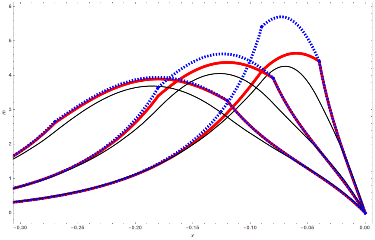
Figure 6: Spatial distribution of the agents, the slim line represents the numerical solution, the thick straight line the approximation using Eq. (75) and the thick dashed line the approximation using only Eq. (88). In this case $T=2$, $a^{(0)}=0.4$, $a^{(2)}=0.9$, $\sigma=0.2$, $\bar{x}_{0}=1.2$ and $\mu=10^{6}$. From left to right, $t=1.9$, $t=1.8$, $t=1.7$.

However, as mentioned in section IV.3, Eq. (75) can be approximated using only Eq. (88). This is shown in Fig. 6 where the results of the two approximations, although obviously different for $t\approx T$ become more and more similar the smaller $t$ gets.

Leak from a constant to a linear drift region

We begin, as in Section IV.3, by computing the position, time and momentum of the agents as they cross the boundary between an region of constant drift $a^{(n)}$ and region (1). Keeping the same notations and using the same method as earlier we have

$$\left\{\begin{aligned} &x^{*(n)}(x_{0})=a^{(n)}(t^{*(n)}-T)=x_{0}(1+t^{*(n)}\mu)+t^{*(n)}(a^{(n)}-\mu x_{0})\\ &t^{*(n)}(x_{0})=\frac{a^{(n)}T+x_{0}}{\mu(\bar{x}_{0}-x_{0})}\\ &p^{*(n)}(x_{0})=\mu(\bar{x}_{0}-x_{0})\\ \end{aligned}\right.\;.$$ (91)

Using the canonical equations in region (1), we compute for $t>t^{*(n)}(x_{0})$

$$\left\{\begin{aligned} &\mathcal{p}^{(n)}(t,x_{0})=\frac{aT+x_{0}-\mu T(\bar{x}_{0}-x_{0})}{t-T}\\ &\mathcal{x}^{(n)}(t,x_{0})=at+x_{0}-\mu t(\bar{x}_{0}-x_{0})\\ &x_{0}(t,x)=\frac{x-at+\mu t\bar{x}_{0}}{1+\mu t}\end{aligned}\right.\;,$$ (92)

from which we get the prefactor

$$\begin{aligned} \frac{\mathcal{N}}{\sqrt{\partial_{x_{0}}\mathcal{x}_{n}(t,x_{0})}}&\exp\left[-\frac{1}{2}\int^{t}_{t^{*(n)}(t,x)}(\partial_{x}a^{(1)})d\tau\right]=\\ &\sqrt{\frac{\mu}{2\pi\sigma^{2}(1+t\mu)}\frac{\mu(t-T)(at-x+\bar{x}_{0})}{a(T-t)+x+\mu Tx-\mu(T-t)\bar{x}_{0}}}\end{aligned}\;,$$ (93)

and the action

$$\begin{aligned} S^{(n)}_{\rm{leak}}(t,x)&=\int^{a^{(n)}(t-T)}_{\mathcal{x}(t,\bar{x}_{0})}p^{(n)}(t,x^{\prime})dx^{\prime}+\int^{x}_{a^{(n)}(t-T)}p^{*(1)}(t,x^{\prime})dx^{\prime}\\ \end{aligned}\;,$$ (94)

with $p^{(n)}$ the constant drift momentum of region (n) given by Eq. (49) and $p^{*(1)}$ the leaking momentum in region (1) obtained by inserting the third equation of Eqs. (92) into the second, yielding

$$\begin{aligned} S^{(n)}_{\rm{leak}}(t,x)&=\frac{1}{2(1+\mu t)(t-T)}\left[-a^{(n)2}(t-T)(T-t+\mu tT)+x^{2}(1+\mu T)\right.\\ &\left.+2\mu(t-T)x\bar{x}_{0}+\mu(T-t)x_{0}^{2}-2a^{(n)}(t-T)(x+\mu t\bar{x}_{0})\right]\end{aligned}\;.$$ (95)

In the case where agents begin in region (2), they may diffuse up to regon (0), using, once again the same scheme, we compute the new prefactor

$$\begin{aligned} \frac{\mathcal{N}}{\sqrt{\partial_{x_{0}}\mathcal{x}_{0}(t,x_{0})}}&\exp\left[-\frac{1}{2}\int^{t^{*(2)}(t,x)}_{t^{*(1)}(t,x)}(\partial_{x}a^{(1)})d\tau\right]=\\ &\sqrt{\frac{\mu}{2\pi\sigma^{2}(1+t\mu)}\frac{\mu(a^{(2)}t-x+\bar{x}_{0})}{a^{(0)}-a^{(2)}+a^{(0)}\mu t+\mu(\bar{x}_{0}-x)}}\end{aligned}\;,$$ (96)

and the new action

$$\begin{aligned} S^{(0)}_{\rm{leak}}(t,x)&=\int^{a^{(2)}(t-T)}_{\mathcal{x}(t,\bar{x}_{0})}p^{(n)}(t,x^{\prime})dx^{\prime}+\int^{a^{(0)}(t-T)}_{a^{(2)}(t-T)}p^{*(1)}(t,x^{\prime})dx^{\prime}+\int^{x}_{a^{(0)}(t-T)}p^{*(0)}(t,x^{\prime})dx^{\prime}\\ &=-\frac{1}{2(1+\mu t)}\left[a^{(2)2}(3+\mu t)(t-T)-a^{(0)2}(T-t+\mu tT)\right.\\ &\left.-2a^{(2)}x+2a^{(0)}\left(-a^{(2)}(2+\mu t)(t-T)+x+\mu t(x-\bar{x}_{0})\right)-\mu(x-\bar{x}_{0})^{2}\right]\end{aligned}\;.$$ (97)

Finally the reflected action is computed as

$$\tilde{S}_{\rm{leak}}(t,x)= S^{(0)}_{\rm{leak}}(t,0)+\int_{0}^{\min[x;a^{(1)}(t-T)]}p^{*(0)}_{-}(t,x^{\prime})dx^{\prime}$$ (98)

$$+\int_{a^{(1)}(t-T)}^{\min\left[\max[x;a^{(1)}(t-T)];a^{(2)}(t-T)\right]}p^{*(1)}_{-}(t,x^{\prime})dx^{\prime}$$

$$+\int_{a^{(2)}(t-T)}^{\max[x,a^{(2)}(t-T)]}p^{(2)}_{-}(t,x^{\prime})dx^{\prime}\;,$$

that we approximate, as in Section IV.3, as

$$\begin{aligned} \tilde{S}_{\rm{leak}}(t,x)&=2a^{(0)}x+\frac{1}{2(1+\mu t)}\left[a^{(2)2}(3+\mu t)(t-T)-a^{(0)2}(T-t+\mu tT)\right.\\ &\left.-2a^{(2)}x+2a^{(0)}\left(-a^{(2)}(2+\mu t)(t-T)+x+\mu t(x-\bar{x}_{0})\right)-\mu(x-\bar{x}_{0})^{2}\right]\end{aligned}\;.$$ (99)

References

- Maslov and Fedoriuk (1981) V. P. Maslov and M. V. Fedoriuk, Semiclassical approximation in quantum mechanics (Reidel Publishing Company, Dordrecht, 1981).
- Lasry and Lions (2006a) J.-M. Lasry and P.-L. Lions, Comptes Rendus Mathematique 343, 619 (2006a).
- Lasry and Lions (2006b) J.-M. Lasry and P.-L. Lions, Comptes Rendus Mathematique 343, 679 (2006b).
- Huang et al. (2006) M. Huang, R. P. Malhamé, P. E. Caines, and others, Communications in Information & Systems 6, 221 (2006).
- Ullmo et al. (2018) D. Ullmo, I. Swiecicki, and T. Gobron, ArXiv:1708.07730 (2018).
- Guéant et al. (2011) O. Guéant, J.-M. Lasry, and P.-L. Lions, in Paris-Princeton Lectures on Mathematical Finance 2010 (Springer, 2011).
- Swiecicki et al. (2016) I. Swiecicki, T. Gobron, and D. Ullmo, Physica A: Statistical Mechanics and its Applications 442, 467 (2016).
- Risken (1996) H. Risken, The Fokker-Planck Equation, 2nd ed. (Springer, 1996).
- Shizgal and Nishigori (1990) B. Shizgal and T. Nishigori, Chemical Physics Letters 171, 493 (1990).
- Derevyanko et al. (2005) S. A. Derevyanko, S. K. Turitsyn, and D. A. Yakushev, J. Opt. Soc. Am. B 22, 743 (2005).
- Caroli et al. (1979) B. Caroli, C. Caroli, and B. Roulet, Journal of Statistical Physics 21, 415 (1979).
- Cohen and Lewis (1967) J. K. Cohen and R. M. Lewis, J. Inst. Maths Applics 3, 266 (1967).
- R. Courant (1962) D. H. R. Courant, Methods of Mathematical Physics, Volume II, ISBN- 10: 0-47 1-50439-4 (Wiley-Interscience, 1962).
- Smirnov (1964) V. I. Smirnov, A Course of Higher Mathematics. Volume IV, ISBN: 978-1-4831-6723-7 (Elsevier, 1964).