$k$-cut on paths and some trees

Abstract

We define the (random) $k$-cut number of a rooted graph to model the difficulty of the destruction of a resilient network. The process is as the cut model of Meir and Moon [21] except now a node must be cut $k$ times before it is destroyed. The first order terms of the expectation and variance of ${\cal X}_{n}$, the $k$-cut number of a path of length $n$, are proved. We also show that ${\cal X}_{n}$, after rescaling, converges in distribution to a limit ${\cal B}_{k}$, which has a complicated representation. The paper then briefly discusses the $k$-cut number of some trees and general graphs. We conclude by some analytic results which may be of interest.

1 Introduction and main results

1.1 The $k$-cut number of a graph

Consider $\mathbb{G}_{n}$, a connected graph consisting of $n$ nodes with exactly one node labeled as the root, which we call a rooted graph. Let $k$ be a positive integer. We remove nodes from the graph as follows:

1. Choose a node uniformly at random from the component that contains the root. Cut the selected node once.

2. If this node has been cut $k$ times, remove the node together with edges attached to it from the graph.

3. If the root has been removed, then stop. Otherwise, go to step 1.

We call the (random) total number of cuts needed to end this procedure the $k$-cut number and denote it by ${\cal K}(\mathbb{G}_{n})$. (Note that in traditional cutting models, nodes are removed as soon as they are cut once, i.e., $k=1$. But in our model, a node is only removed after being cut $k$ times.)

One can also define an edge version of this process. Instead of cutting nodes, each time we choose an edge uniformly at random from the component that contains the root and cut it once. If the edge has been cut $k$-times then we remove it. The process stops when the root is isolated. We let ${\cal K}_{e}(\mathbb{G}_{n})$ denote the number of cuts needed for the process to end.

Our model can also be applied to botnets, i.e., malicious computer networks consisting of compromised machines which are often used in spamming or attacks. The nodes in $\mathbb{G}_{n}$ represent the computers in a botnet, and the root represents the bot-master. The effectiveness of a botnet can be measured using the size of the component containing the root, which indicates the resources available to the bot-master [6]. To take down a botnet means to reduce the size of this root component as much as possible. If we assume that we target infected computers uniformly at random and it takes at least $k$ attempts to fix a computer, then the $k$-cut number measures how difficult it is to completely isolate the bot-master.

The case $k=1$ and $\mathbb{G}_{n}$ being a rooted tree has aroused great interests among mathematicians in the past few decades. The edge version of one-cut was first introduced by [21] for the uniform random Cayley tree. [16] [16, 17] noticed the equivalence between one-cuts and records in trees and studied them in binary trees and conditional Galton-Watson trees. Later [1] gave a simpler proof for the limit distribution of one-cuts in conditional Galton-Watson trees. For one-cuts in random recursive trees, see [22, 15, 9]. For binary search trees and split trees, see [12, 13].

1.2 The $k$-cut number of a tree

One of the most interesting cases is when $\mathbb{G}_{n}=\mathbb{T}_{n}$, where $\mathbb{T}_{n}$ is a rooted tree with $n$ nodes.

There is an equivalent way to define ${\cal K}(\mathbb{T}_{n})$. Imagine that each node is given an alarm clock. At time zero, the alarm clock of node $v$ is set to ring at time $T_{1,v}$, where $(T_{i,v})_{i\geq 1,v\in\mathbb{T}_{n}}$ are i.i.d. (independent and identically distributed) $\mathop{\mathrm{Exp}}(1)$ random variables. After the alarm clock of node $v$ rings the $i$-th time, we set it to ring again at time $T_{i+1,v}$. Due to the memoryless property of exponential random variables (see [10, pp. 134]), at any moment, which alarm clock rings next is always uniformly distributed. Thus, if we cut a node that is still in the tree when its alarm clock rings, and remove the node with its descendants if it has already been cut $k$-times, then we get exactly the $k$-cut model. (The random variables $(T_{i,v})_{i\geq 1}$ can be seen as the holding times in a Poisson process $N(t)_{v}$ of parameter $1$, where $N(t)_{v}$ is the number of cuts in $v$ during the time $[0,t]$ and has a Poisson distribution with parameter $t$.)

How can we tell if a node is still in the tree? When node $v$’s alarm clock rings for the $r$-th time for some $r\leq k$, and no node above $v$ has already rung $k$ times, we say $v$ has become an $r$-record. And when a node becomes an $r$-record, it must still be in the tree. Thus, summing the number of $r$-records over $r\in\{1,\dots,k\}$, we again get the $k$-cut number ${\cal K}(\mathbb{T}_{n})$. One node can be a $1$-record, a $2$-record, etc., at the same time, so it can be counted multiple times. Note that if a node is an $r$-record, then it must also be a $i$-record for $i\in\{1,\dots,r-1\}$.

To be more precise, we define ${\cal K}(\mathbb{T}_{n})$ as a function of $(T_{i,v})_{i\geq 1,v\geq 1}$. Let

$$G_{r,v}\,{\buildrel{\mathrm{def}}\over{=}}\,\sum_{i=1}^{r}T_{i,v},$$ (1.1)

i.e., $G_{r,v}$ is the moment when the alarm clock of node $v$ rings for the $r$-th time. Then $G_{r,v}$ has a gamma distribution with parameters $(r,1)$ (see [10, Theorem 2.1.12]), which we denote by $\mathop{\mathrm{Gamma}}(r)$. Let

$$I_{r,v}\,{\buildrel{\mathrm{def}}\over{=}}\,\llbracket G_{r,v}<\min\{G_{k,u}:u\in\mathbb{T}_{n},\text{$u$ is an ancestor of $v$}\}\rrbracket,$$ (1.2)

where $\llbracket\cdot\rrbracket$ denotes the Iverson bracket, i.e., $\llbracket S\rrbracket=1$ if the statement $S$ is true and $\llbracket S\rrbracket=0$ otherwise. In other words, $I_{r,v}$ is the indicator random variable for node $v$ being an $r$-record. Let

$${\cal K}_{r}(\mathbb{T}_{n})\,{\buildrel{\mathrm{def}}\over{=}}\,\sum_{v\in\mathbb{T}_{n}}I_{r,v},\qquad{\cal K}(\mathbb{T}_{n})\,{\buildrel{\mathrm{def}}\over{=}}\,\sum_{r=1}^{k}{\cal K}_{r}(\mathbb{T}_{n}).$$

Then ${\cal K}_{r}(\mathbb{T}_{n})$ is the number of $r$-records and ${\cal K}(\mathbb{T}_{n})$ is the total number of records.

1.3 The $k$-cut number of a path

Let $\mathbb{P}_{n}$ be a one-ary tree (a path) consisting of $n$ nodes labeled $1,\dots,n$ from the root to the leaf. To simplify notations, from now on we use $I_{r,i},G_{r,i}$, and $T_{r,i}$ to represent $I_{r,v},G_{r,v}$ and $T_{r,v}$ respectively for a node $v$ at depth $i$.

Let ${\cal X}_{n}\,{\buildrel{\mathrm{def}}\over{=}}\,{\cal K}(\mathbb{P}_{n})$ and ${\cal X}_{n,r}={\cal K}_{r}(\mathbb{P}_{n})$. In this paper, we mainly consider ${\cal X}_{n}$ and we let $k\geq 2$ be a fixed integer.

The first motivation of this choice is that, as shown in Section 4, $\mathbb{P}_{n}$ is the fastest to cut among all graphs. (We make this statement precise in Lemma 10.) Thus ${\cal X}_{n}$ provides a universal stochastic lower bound for ${\cal K}(\mathbb{G}_{n})$. Moreover, our results on ${\cal X}_{n}$ can immediately be extended to some trees of simple structures: see Section 4. Finally, as shown below, ${\cal X}_{n}$ generalizes the well-known record number in permutations and has very different behavior when $k=1$, the usual cut-model, and $k\geq 2$, our extended model.

The name record comes from the classic definition of records in random permutations. Let $\sigma_{1},\dots,\sigma_{n}$ be a uniform random permutation of $\{1,\dots,n\}$. If $\sigma_{i}<\min_{1\leq j<i}\sigma_{j}$, then $i$ is called a (strictly lower) record. Let ${\cal R}_{n}$ denote the number of records in $\sigma_{1},\dots,\sigma_{n}$. Let $W_{1},\dots,W_{n}$ be i.i.d. random variables with a common continuous distribution. Since the relative order of $W_{1},\dots,W_{n}$ also gives a uniform random permutation, we can equivalently define $\sigma_{i}$ as the rank of $W_{i}$. As gamma distributions are continuous, we can in fact let $W_{i}=G_{k,i}$. Thus, being a record in a uniform permutation is equivalent to being a $k$-record and ${\cal R}_{n}\,{\buildrel{\cal L}\over{=}}\,{\cal X}_{n,k}$. Moreover, when $k=1$, ${\cal R}_{n}\,{\buildrel{\cal L}\over{=}}\,{\cal X}_{n}$.

Starting from [5]’s article [5] in chandler52, the theory of records has been widely studied due to its applications in statistics, computer science, and physics. For more recent surveys on this topic, see [2].

A well-known result of ${\cal R}_{n}$ (and thus also ${\cal X}_{n,k}$) [25] is that $(I_{k,j})_{1\leq j\leq n}$ are independent. It follows from the Lindeberg–Lévy–Feller Theorem that

$$\frac{{\mathbf{E}}\left[{\cal R}_{n}\right]}{\log n}\to 1,\qquad\frac{{\cal R}_{n}}{\log n}\,{\buildrel{a.s.}\over{\rightarrow}}\,1,\qquad{\cal L}\left(\frac{{\cal R}_{n}-\log n}{\sqrt{\log n}}\right){\,{\buildrel d\over{\rightarrow}}\,}{\cal N}(0,1),$$ (1.3)

where ${\cal N}(0,1)$ denotes the standard normal distribution.

In the following, Theorem 1 gives the expectation of ${\cal X}_{n,r}$ which implies that the number of one-records dominates the number of other records. Subsequently Theorem 2 and Theorem 3 estimate the variance and higher moments of ${\cal X}_{n,1}$.

Theorem 1.

For all fixed $k\in{\mathbb{N}}$,

$${\mathbf{E}}\left[{\cal X}_{n,r}\right]\sim\left\{\begin{array}[]{*2{>{\displaystyle}l}}\eta_{k,r}n^{1-\frac{r}{k}}&(1\leq r<k),\\ \log n&(r=k),\end{array}\right.$$ (1.6)

where the constants $\eta_{k,r}$ are defined by

$$\eta_{k,r}\,{\buildrel{\mathrm{def}}\over{=}}\,\frac{(k!)^{\frac{r}{k}}}{k-r}\frac{\Gamma\left(\frac{r}{k}\right)}{\Gamma(r)},$$ (1.7)

where $\Gamma(z)$ denotes the gamma function. Therefore ${\mathbf{E}}\left[{\cal X}_{n}\right]\sim{\mathbf{E}}\left[{\cal X}_{n,1}\right]$. Also, for $k=2$,

$${\mathbf{E}}\left[{\cal X}_{n}\right]\sim{\mathbf{E}}\left[{\cal X}_{n,1}\right]\sim\sqrt{2\pi n}.$$

Theorem 2.

For all fixed $k\in\{2,3,\dots\}$,

$${\mathbf{E}}\left[{\cal X}_{n,1}({\cal X}_{n,1}-1)\right]\sim{\mathbf{E}}\left[\left({\cal X}_{n,1}\right)^{2}\right]\sim\gamma_{k}n^{2-\frac{2}{k}},$$ (1.8)

where

$$\gamma_{k}=\frac{\Gamma\left(\frac{2}{k}\right)(k!)^{\frac{2}{k}}}{k-1}+2\lambda_{k},$$ (1.9)

and

$$\lambda_{k}=\left\{\begin{array}[]{*2{>{\displaystyle}l}}\frac{\pi\cot\left(\frac{\pi}{k}\right)\Gamma\left(\frac{2}{k}\right)(k!)^{\frac{2}{k}}}{2\left({k}-2\right)\left({k}-1\right)}&k>2,\\ \frac{\pi^{2}}{4}&k=2.\end{array}\right.$$ (1.12)

Therefore

$${\mathrm{Var}}\left({\cal X}_{n,1}\right)\sim\left(\gamma_{k}-\eta_{k,1}^{2}\right)n^{2-\frac{2}{k}}.$$ (1.13)

In particular, when $k=2$

$${\mathrm{Var}}\left({\cal X}_{n,1}\right)\sim\left(\frac{\pi^{2}}{2}+2-2\pi\right)n.$$ (1.14)

Theorem 3.

For all fixed $k\in\{2,3,\dots\}$ and $\ell\in{\mathbb{N}}$

$$\limsup_{n\to\infty}{\mathbf{E}}\left[\left(\frac{{\cal X}_{n,1}}{n^{1-\frac{1}{k}}}\right)^{\ell}\right]\leq\rho_{k,\ell}\,{\buildrel{\mathrm{def}}\over{=}}\,{\ell!}{\Gamma\left(\ell+1-\frac{\ell}{k}\right)^{-1}}\left(\frac{\pi}{k}(k!)^{1/k}\sin\left(\frac{\pi}{k}\right)^{-1}\right)^{\ell}.$$ (1.15)

The upper bound is tight for $\ell=1$ since $\rho_{k,1}=\eta_{k,1}$.

The above theorems imply that the correct rescaling parameter should be ${n^{1-\frac{1}{k}}}$. However, unlike the case $k=1$, when $k\geq 2$ the limit distribution of ${\cal X}_{n}/{n^{1-\frac{1}{k}}}$ has a rather complicated representation ${\cal B}_{k}$ defined as follows: Let $U_{1},E_{1},U_{2},E_{2},\dots$ be mutually independent random variables with $E_{j}\,{\buildrel{\cal L}\over{=}}\,\mathop{\mathrm{Exp}}(1)$ and $U_{j}\,{\buildrel{\cal L}\over{=}}\,\mathop{\mathrm{Unif}}[0,1]$. Let

$$S_{p}\,{\buildrel{\mathrm{def}}\over{=}}\,\left(k!\sum_{1\leq s\leq p}\left(\prod_{s\leq j<p}U_{j}\right)E_{s}\right)^{\frac{1}{k}},$$ (1.16)

$$B_{p}\,{\buildrel{\mathrm{def}}\over{=}}\,\left(1-U_{p}\right)\left(\prod_{1\leq j<p}U_{j}\right)^{1-\frac{1}{k}}S_{p},$$ (1.17)

$${\cal B}_{k}\,{\buildrel{\mathrm{def}}\over{=}}\,\sum_{1\leq p}B_{p},$$ (1.18)

where we use the convention that an empty product equals one.

Remark 1.

An equivalent recursive definition of $S_{p}$ is

$$S_{p}=\begin{cases}k!E_{1}&(p=1),\\ \left(U_{p-1}S_{p-1}^{k}+k!E_{p}\right)^{\frac{1}{k}}\qquad\qquad&(p\geq 2).\end{cases}$$ (1.19)

Theorem 4.

Let $k\in\{2,3,\dots\}$. Let ${\cal L}({\cal B}_{k})$ denote the distribution of ${\cal B}_{k}$. Then

$${\cal L}\left(\frac{{\cal X}_{n}}{{n^{1-\frac{1}{k}}}}\right){\,{\buildrel d\over{\rightarrow}}\,}{\cal L}({\cal B}_{k}).$$ (1.20)

Thus, by Theorem 1, 2 and 3, the convergence also holds in $L^{p}$ for all $p>0$ and

$${\mathbf{E}}\left[{\cal B}_{k}\right]=\eta_{k,1},\qquad{\mathbf{E}}\left[{\cal B}_{k}^{2}\right]=\gamma_{k},\qquad{\mathbf{E}}\left[{\cal B}_{k}^{p}\right]\in[\eta_{k,1}^{p},\rho_{k,p}]\qquad(p\in{\mathbb{N}}).$$ (1.21)

Remark 2.

The idea behind ${\cal B}_{k}$ is that we split the path into segments according to the positions of $k$-records, then count the numbers of one-records in every segment, each of which converges to a $B_{p}$ in the sum (1.18). This will be made rigorous in Section 3. We will also see that ${\cal B}_{k}$ has a density close to a normal distribution in Section 3.4.

Remark 3.

It is easy to see that ${\cal X}_{n+1}^{\mathrm{e}}\,{\buildrel{\mathrm{def}}\over{=}}\,{\cal K}_{e}(P_{n+1})\,{\buildrel{\cal L}\over{=}}\,{\cal X}_{n}$ by treating each edge on a length $n+1$ path as a node on a length $n$ path.

The rest of the paper is organized as follows: Section 2 proves the moment results Theorem 1, 2, and 3. Section 3 deals with the distributional result Theorem 4. Section 4 discusses some easy results for general graphs and trees. Finally, Section 5 collects analytic results used in the proofs, which may themselves be of interest.

2 The moments

2.1 The expectation

In this section we prove Theorem 1.

Lemma 1.

Uniformly for all $i\geq 1$ and $r\in\{1,\dots,k\}$,

$${\mathbf{E}}\left[I_{r,i+1}\right]=\left(1+{O\!\left(i^{-\frac{1}{2k}}\right)}\right)\frac{(k!)^{\frac{r}{k}}}{k}\frac{\Gamma\left(\frac{r}{k}\right)}{\Gamma(r)}i^{-\frac{r}{k}}.$$ (2.1)

Proof.

By (1.2), ${\mathbf{E}}\left[I_{r,i+1}\right]={\mathbf{P}}\left\{G_{k,1}>G_{r,i+1},\dots,G_{k,i}>G_{r,i+1}\right\}$. Conditioning on $G_{r,i+1}=x$ yields ${\mathbf{E}}\left[I_{r,i+1}\right]=\int_{0}^{\infty}{x^{r-1}{\mathrm{e}}^{-x}}/{\Gamma(r)}{\mathbf{P}}\left\{G_{k,1}>x\right\}^{i}\,\mathrm{d}x$. Lemma 1 thus follows from Lemma 17. ∎

Proof of Theorem 1.

A simply computation shows that for $a\in(0,1)$

$$\sum_{1\leq i\leq n}\frac{1}{i^{a}}=\frac{1}{1-a}n^{1-a}+O(1).$$ (2.2)

It then follows from Lemma 1 that for $r\in\{1,\dots,k-1\}$.

$${\mathbf{E}}\left[{\cal X}_{n,r}\right]=\sum_{0\leq i<n}{\mathbf{E}}\left[I_{r,i+1}\right]=\frac{(k!)^{\frac{r}{k}}}{k}\frac{\Gamma\left(\frac{r}{k}\right)}{\Gamma(r)}\frac{1}{1-\frac{r}{k}}n^{1-\frac{r}{k}}+{O\!\left(n^{1-\frac{r}{k}-\frac{1}{2k}}\right)}+{O\!\left(1\right)}.$$ (2.3)

When $r=k$, ${\mathbf{E}}\left[{\cal X}_{n,k}\right]={\mathbf{E}}\left[{\cal R}_{n}\right]\sim\log(n)$ is already well-known. ∎

2.2 The variance

In this section we prove Theorem 2.

Let $E_{i,j}$ denote the event that $[I_{1,i+1}I_{1,j+1}=1]$. Let $A_{x,y}$ denote the event that $[G_{1,i+1}=x\cap G_{1,j+1}=y]$. Then conditioning on $A_{x,y}$

$$E_{i,j}=\left[\bigcap_{1\leq s\leq i}G_{k,s}>x\vee y\right]\cap\left[G_{k,i+1}>y\right]\cap\left[\bigcap_{i+2\leq s\leq j}G_{k,s}>y\right],$$ (2.4)

where $x\vee y\,{\buildrel{\mathrm{def}}\over{=}}\,\max\{x,y\}$. Since conditioning on $A_{x,y}$, $G_{k,i+1}\,{\buildrel{\cal L}\over{=}}\,\mathop{\mathrm{Gamma}}(k-1)+x$, $G_{k,s}\,{\buildrel{\cal L}\over{=}}\,\mathop{\mathrm{Gamma}}(k)$ for $s\notin\{i+1,j+1\}$, and all these random variables are independent, we have

$${\mathbf{P}}\left\{E_{i,j}|A_{x,y}\right\}={\mathbf{P}}\left\{G_{k-1,1}+x>y\right\}{\mathbf{P}}\left\{G_{k,1}>x\vee y\right\}^{i}{\mathbf{P}}\left\{G_{k,1}>y\right\}^{j-i-1}.$$ (2.5)

It follows from $G_{1,i+1}\,{\buildrel{\cal L}\over{=}}\,G_{1,j+1}\,{\buildrel{\cal L}\over{=}}\,\mathop{\mathrm{Exp}}(1)$ that

$${\mathbf{P}}\left\{E_{i,j}\right\} =\int_{0}^{\infty}\int_{y}^{\infty}{\mathrm{e}}^{-x-y}{\mathbf{P}}\left\{E_{i,j}|A_{x,y}\right\}\,\mathrm{d}x\,\mathrm{d}y$$ (2.6)

$$\qquad+\int_{0}^{\infty}\int_{0}^{y}{\mathrm{e}}^{-x-y}{\mathbf{P}}\left\{E_{i,j}|A_{x,y}\right\}\,\mathrm{d}x\,\mathrm{d}y$$ (2.7)

$$\,{\buildrel{\mathrm{def}}\over{=}}\,A_{1,i,j}+A_{2,i,j}.$$ (2.8)

We next estimate these two terms.

Lemma 2.

Let $k\in\{2,3,\dots\}$. We have

$$A_{2,i,j}=\left(1+{O\!\left(j^{-\frac{1}{2k}}\right)}\right)\frac{(k!)^{\frac{2}{k}}}{k}{\Gamma\left(\frac{2}{k}\right)}j^{-\frac{2}{k}}.$$ (2.9)

Proof.

In this case, $x\vee y=y$. Thus, by (2.5)

$$A_{2,i,j}=\int_{0}^{\infty}{\mathrm{e}}^{-y}{\mathbf{P}}\left\{G_{k,1}>y\right\}^{j-1}\int_{0}^{y}{\mathrm{e}}^{-x}{\mathbf{P}}\left\{G_{k-1,1}>y-x\right\}\,\mathrm{d}x\,\mathrm{d}y.$$ (2.10)

Note that the dependence on $i$ disappears. Let $Z$ denote a Poisson random variable with mean $y-x$. By the well-known connection between Poisson and gamma distributions, the inner integral in the above equals

$$\int_{0}^{y}{\mathrm{e}}^{-x}{\mathbf{P}}\left\{Z<k-1\right\}\,\mathrm{d}x=\int_{0}^{y}{\mathrm{e}}^{-x}\sum_{\ell=0}^{k-2}{\mathrm{e}}^{-(y-x)}\frac{(y-x)^{\ell}}{\ell!}\,\mathrm{d}x={\mathrm{e}}^{-y}\sum_{\ell=0}^{k-2}\frac{y^{\ell+1}}{(\ell+1)!}.$$ (2.11)

It then follows from Lemma 17 that

$$A_{2,i,j} =\sum_{\ell=0}^{k-2}\int_{0}^{\infty}{\mathrm{e}}^{-2y}\frac{y^{\ell+1}}{(\ell+1)!}{\mathbf{P}}\left\{G_{k,1}>y\right\}^{j-1}\,\mathrm{d}y$$ (2.12)

$$=\sum_{\ell=0}^{k-2}\left(1+{O\!\left(j^{-\frac{1}{2k}}\right)}\right)\frac{\left(k!\right)^{\frac{\ell+2}{k}}}{k(\ell+1)!}\Gamma\left(\frac{\ell+2}{k}\right)j^{-\frac{\ell+2}{k}}$$ (2.13)

$$=\left(1+{O\!\left(j^{-\frac{1}{2k}}\right)}\right)\frac{(k!)^{\frac{2}{k}}}{k}{\Gamma\left(\frac{2}{k}\right)}j^{-\frac{2}{k}}.\qed$$ (2.14)

Lemma 3.

Let $k\in\{2,3,\dots\}$. Let $a=i$ and $b=j-i-1$. Then for all $a\geq 1$ and $b\geq 1$,

$$A_{1,i,j}=\xi_{k}(a,b)+{O\!\left(\left(a^{-\frac{1}{2k}}+b^{-\frac{1}{2k}}\right)\left(a^{-\frac{2}{k}}+b^{-\frac{2}{k}}\right)\right)},$$ (2.15)

where

$$\xi_{k}(a,b)\,{\buildrel{\mathrm{def}}\over{=}}\,\int_{0}^{\infty}\int_{y}^{\infty}\exp\left(-a\frac{x^{k}}{k!}-b\frac{y^{k}}{k!}\right)\,\mathrm{d}x\,\mathrm{d}y.$$ (2.16)

Proof.

In this case, $x\vee y=x$ and $y-x<0$. Thus, by (2.5) and Lemma 17

$$A_{1,i,j} =\int_{0}^{\infty}\int_{y}^{\infty}{\mathrm{e}}^{-x}{\mathrm{e}}^{-y}{\mathbf{P}}\left\{G_{k,1}>x\right\}^{i}{\mathbf{P}}\left\{G_{k,1}>y\right\}^{j-i-1}\,\mathrm{d}x\,\mathrm{d}y$$ (2.17)

$$=\int_{0}^{\infty}\int_{y}^{\infty}{\mathrm{e}}^{-x-y}\left(\frac{\Gamma(k,x)}{\Gamma\left(k\right)}\right)^{a}\left(\frac{\Gamma(k,y)}{\Gamma\left(k\right)}\right)^{b}\,\mathrm{d}x\,\mathrm{d}y,$$ (2.18)

where $\Gamma(\ell,z)$ denotes the upper incomplete gamma function.

Let ${\cal S}$ be the integration area of (2.18). Let $x_{0}=a^{-\alpha}$ and $y_{0}=b^{-\alpha}$ where $\alpha=\frac{1}{2}\left(\frac{1}{k}+\frac{1}{k+1}\right)$. Let

$${\cal S}_{0}={\cal S}\cap\left\{(x,y)\in{\mathbb{R}}^{2}:x<x_{0},y<y_{0}\right\}.$$ (2.19)

We split (2.18) into two parts $A_{1,1}$ and $A_{1,2}$ with integration area ${\cal S}_{0}$ and ${\cal S}\setminus{\cal S}_{0}$ respectively.

Let $\beta=\frac{1}{2(k+1)}$. Let $x_{1}=a^{\beta}/k!$ and $y_{1}=b^{\beta}/k!$. It follows from Lemma 16 and Lemma 19 that

$$A_{1,1} =\left(1+{O\!\left(a^{-\frac{1}{2k}}+b^{-\frac{1}{2k}}\right)}\right)\iint_{{\cal S}_{0}}\exp\left(-a\frac{x^{k}}{k!}-b\frac{y^{k}}{k!}\right)\,\mathrm{d}x\,\mathrm{d}y$$ (2.20)

$$=\left(1+{O\!\left(a^{-\frac{1}{2k}}+b^{-\frac{1}{2k}}\right)}\right)\xi_{k}(a,b)+{O\!\left({\mathrm{e}}^{-x_{1}}+{\mathrm{e}}^{-y_{1}}\right)}$$ (2.21)

$$=\xi_{k}(a,b)+{O\!\left(\left(a^{-\frac{1}{2k}}+b^{-\frac{1}{2k}}\right)\left(a^{-\frac{2}{k}}+b^{-\frac{2}{k}}\right)\right)}+{O\!\left({\mathrm{e}}^{-x_{1}}+{\mathrm{e}}^{-y_{1}}\right)}.$$ (2.22)

It is not difficult to verify that

$$A_{1,2}={O\!\left(\left(\frac{\Gamma(k,x_{0})}{\Gamma(k)}\right)^{-a}+\left(\frac{\Gamma(k,y_{0})}{\Gamma(k)}\right)^{-b}\right)}={O\!\left({\mathrm{e}}^{-x_{1}}+{\mathrm{e}}^{-y_{1}}\right)}.$$ (2.23)

The lemma follows since ${\mathrm{e}}^{-x_{1}}+{\mathrm{e}}^{-y_{1}}$ is exponentially small. ∎

Proof of Theorem 2.

We have

$${\mathbf{E}}\left[{\cal X}_{n,1}\left({\cal X}_{n,1}-1\right)\right]=2\sum_{i=1}^{n-1}\sum_{j=i+1}^{n}{\mathbf{P}}\left\{E_{i,j}\right\}=2\sum_{i=0}^{n-2}\sum_{j=i+1}^{n-1}\left(A_{1,i,j}+A_{2,i,j}\right).$$ (2.24)

Thus, by Lemma 2 and (2.2),

$$\sum_{i=0}^{n-2}\sum_{j=i+1}^{n-1}A_{2,i,j} =\sum_{i=0}^{n-2}\sum_{j=i+1}^{n-1}\left[\frac{(k!)^{\frac{2}{k}}{\Gamma\left(\frac{2}{k}\right)}}{k}j^{-\frac{2}{k}}+{O\!\left(j^{-\frac{5}{2k}}\right)}\right]$$ (2.25)

$$=\frac{(k!)^{\frac{2}{k}}\Gamma\left(\frac{2}{k}\right)}{2(k-1)}n^{2-\frac{2}{k}}+{O\!\left(n^{2-\frac{5}{2k}}\right)}.$$ (2.26)

For $A_{1,i,j}$, it follows from Lemma 3 that

$$\sum_{i=0}^{n-2}\sum_{j=i+1}^{n-1}A_{1,i,j} =\sum_{a=1}^{n-1}\,\sum_{b=1}^{n-a}\xi_{k}(a,b)+{O\!\left(n^{2-\frac{5}{2k}}\right)}$$ (2.27)

$$=\int_{0}^{n}\,\int_{0}^{n-a}\xi_{k}(a,b)\,\mathrm{d}b\,\mathrm{d}a+{O\!\left(n^{2-\frac{5}{2k}}\right)}$$ (2.28)

$$=n^{2-\frac{2}{k}}\int_{0}^{1}\,\int_{0}^{1-s}\xi_{k}(s,t)\,\mathrm{d}t\,\mathrm{d}s+{O\!\left(n^{2-\frac{5}{2k}}\right)}$$ (2.29)

$$=\lambda_{k}n^{2-\frac{2}{k}}+{O\!\left(n^{2-\frac{5}{2k}}\right)},$$ (2.30)

where the last step follows from Lemma 20. Theorem 2 follows by putting (2.26), (2.30) into (2.24). ∎

2.3 Higher moments

In this section we prove Theorem 3.

The computations of higher moments of ${\cal X}_{n,1}$ are rather complicated. However, an upper bound is readily available. Let $(x)_{\ell}\,{\buildrel{\mathrm{def}}\over{=}}\,x(x-1)\dots(x-\ell+1)$. For $\ell\geq 1$,

$${\mathbf{E}}\left[({\cal X}_{n,1})_{\ell}\right] =\ell!\sum_{1\leq i_{1}<i_{2}\dots<i_{\ell}\leq n}{\mathbf{E}}\left[I_{1,i_{1}}I_{1,i_{2}}\cdots I_{1,i_{\ell}}\right]$$

$$\leq\ell!\sum_{1\leq i_{1}<i_{2}\dots<i_{\ell}\leq n}{\mathbf{E}}\left[I_{1,i_{1}}\right]{\mathbf{E}}\left[I_{1,i_{2}-i_{1}}\right]\cdots{\mathbf{E}}\left[I_{1,i_{\ell}-i_{\ell-1}}\right]$$

$$=\ell!\sum_{(a_{1},\dots,a_{\ell})\in{\cal S}_{n,\ell}}\prod_{j=1}^{\ell}{\mathbf{E}}\left[I_{1,a_{j}}\right],$$ (2.31)

where

$${\cal S}_{n,\ell}\,{\buildrel{\mathrm{def}}\over{=}}\,\left\{(a_{1},a_{2},\dots,a_{\ell})\in{\mathbb{N}}^{\ell}:a_{1}\geq 0,\dots,a_{\ell}\geq 0,\sum_{j=1}^{\ell}a_{j}\leq n-\ell\right\}.$$ (2.32)

The above inequality holds since if $i_{j}$ is a one-record in the whole path, then it must also be a one-record in the segment $(i_{j-1}+1,\dots,i_{j})$ ignoring everything else, and what happens in each of such segments are independent. It follows from Lemma 1 that (2.31) equals

$$\ell!\sum_{(a_{1},\dots,a_{\ell})\in{\cal S}_{n,\ell}}\prod_{j=1}^{\ell}\left(1+{O\!\left(a_{j}^{-\frac{1}{2k}}\right)}\right)\frac{(k!)^{\frac{1}{k}}}{k}\Gamma\left(\frac{1}{k}\right)a_{j}^{-\frac{1}{k}}$$ (2.33)

$$=\ell!n^{\ell\left(1-\frac{1}{k}\right)}\left(\frac{(k!)^{\frac{1}{k}}}{k}\Gamma\left(\frac{1}{k}\right)\right)^{\ell}\sum_{(a_{1},\dots,a_{\ell})\in{\cal S}_{n,\ell}}\prod_{j=1}^{\ell}\left(1+{O\!\left(a_{j}^{-\frac{1}{2k}}\right)}\right)\left(\frac{a_{j}}{n}\right)^{-\frac{1}{k}}\frac{1}{n}$$

$$\sim n^{\ell\left(1-\frac{1}{k}\right)}\ell!\left(\frac{(k!)^{\frac{1}{k}}}{k}\Gamma\left(\frac{1}{k}\right)\right)^{\ell}\int_{A_{\ell}}\prod_{j=1}^{\ell}x_{j}^{-\frac{1}{k}}\,\mathrm{d}(x_{1},\dots,x_{\ell})$$

$$=n^{\ell\left(1-\frac{1}{k}\right)}\ell!\left(\frac{(k!)^{\frac{1}{k}}}{k}\Gamma\left(\frac{1}{k}\right)\right)^{\ell}\zeta_{k,\ell}=n^{\ell\left(1-\frac{1}{k}\right)}\rho_{k,\ell},$$

where $A_{\ell}$ is the simplex $\{(x_{1},\dots,x_{\ell}):x_{1}>0,\dots,x_{\ell}>0,x_{1}+\dots+x_{\ell}<1\},$ and

$$\zeta_{k,\ell}\,{\buildrel{\mathrm{def}}\over{=}}\,{\Gamma\left(\frac{k-1}{k}\right)^{\ell}}{\Gamma\left(1+\ell-\frac{\ell}{k}\right)^{-1}}.$$ (2.34)

The above integral is known as the beta integral [24, 5.14.1].

3 Convergence to the $k$-cut distribution

By Theorem 1 and Markov’s inequality, ${{\cal X}_{n,r}}/{{n^{1-\frac{1}{k}}}}{\,{\buildrel p\over{\rightarrow}}\,}0$ for $r\in\{2,\dots,k\}$. So it suffices to prove Theorem 4 for ${\cal X}_{n,1}$ instead of ${\cal X}_{n}$. Throughout Section 3, unless otherwise emphasized, we assume that $k\geq 2$.

The idea of the proof is to condition on the positions and values of the $k$-records, and study the distribution of the number of one-records between two consecutive $k$-records.

We use $(R_{n,p})_{p\geq 1}$ to denote the $k$-record values and $(P_{n,p})_{p\geq 1}$ the positions of these $k$-records. To be precise, let $R_{n,0}\,{\buildrel{\mathrm{def}}\over{=}}\,0$, and $P_{n,0}\,{\buildrel{\mathrm{def}}\over{=}}\,n+1$; for $p\geq 1$, if $P_{n,p-1}>1$, then let

$$R_{n,p}\,{\buildrel{\mathrm{def}}\over{=}}\,\min\{G_{k,j}:{1\leq j<P_{n,p-1}}\},$$ (3.1)

$$P_{n,p}\,{\buildrel{\mathrm{def}}\over{=}}\,\operatornamewithlimits{argmin}\{G_{k,j}:{1\leq j<P_{n,p-1}}\},$$

i.e., $P_{n,p}$ is the unique positive integer which satisfies that $G_{k,P_{n,p}}\leq G_{k,i}$ for all $1\leq i<P_{n,p-1}$; otherwise let $P_{n,p}=1$ and $R_{n,p}=\infty$. Note that $R_{n,1}$ is simply the minimum of $n$ i.i.d. $\mathop{\mathrm{Gamma}}(k)$ random variables.

According to $(P_{n,p})_{p\geq 1}$, we split ${\cal X}_{n,1}$ into the following sum

$${\cal X}_{n,1}=\sum_{1\leq j\leq n}I_{1,j}={\cal X}_{n,k}+\sum_{1\leq p}\sum_{1\leq j}\,\llbracket P_{n,p-1}>j>P_{n,p}\rrbracket\,I_{1,j}\,{\buildrel{\mathrm{def}}\over{=}}\,{\cal X}_{n,k}+\sum_{1\leq p}B_{n,p}.$$ (3.2)

Figure 1 gives an example of $(B_{n,p})_{p\geq 1}$ for $n=12$. It depicts the positions of the $k$-records and the one-records. It also shows the values and the summation ranges for $(B_{n,p})_{p\geq 1}$.

Figure 1: An example of $(B_{n,p})_{p\geq 1}$ for $n=12$.

Recall that $T_{r,j}\,{\buildrel{\cal L}\over{=}}\,\mathop{\mathrm{Exp}}(1)$, is the lapse of time between the alarm clock of $j$ rings for the $(r-1)$-st time and the $r$-th time. Conditioning on $(R_{n,p},P_{n,p})_{n\geq 1,p\geq 1}$, for $j\in(P_{n,p},P_{n,p-1})$, we have

$${\mathbf{E}}\left[I_{1,j}\right] ={\mathbf{P}}\left\{T_{1,j}<R_{n,p}\left|G_{k,j}>R_{n,p-1}\right.\right\}.$$ (3.3)

Then the distribution of $B_{n,p}{}$ conditioning on $(R_{n,p},P_{n,p})_{n\geq 1,p\geq 1}$ is simply that of

$$\mathop{\mathrm{Bin}}\left(P_{n,p-1}-P_{n,p}-1,{\mathbf{P}}\left\{T_{1,j}<R_{n,p}\left|G_{k,j}>R_{n,p-1}\right.\right\}\right),$$ (3.4)

where $\mathop{\mathrm{Bin}}(m,p)$ denotes a binomial $(m,p)$ random variable. When $R_{n,p-1}$ is small and $P_{n,p-1}-P_{n,p}$ is large, this is roughly

$$\mathop{\mathrm{Bin}}\left(P_{n,p-1}-P_{n,p},{\mathbf{P}}\left\{T_{1,j}<R_{n,p}\right\}\right)\,{\buildrel{\cal L}\over{=}}\,\mathop{\mathrm{Bin}}\left(P_{n,p-1}-P_{n,p},1-{\mathrm{e}}^{-R_{n,p}}\right).$$ (3.5)

Therefore, we first study a slightly simplified model. Let $(T^{*}_{r,j})_{r\geq 1,j\geq 1}$ be i.i.d. $\mathop{\mathrm{Exp}}(1)$ which are also independent from $(T_{r,j})_{r\geq 1,j\geq 1}$. Let

$$I^{*}_{j}\,{\buildrel{\mathrm{def}}\over{=}}\,\llbracket T^{*}_{1,j}<\min\{G_{k,i}:1\leq i\leq j\}\rrbracket,\qquad{\cal X}^{*}_{n}\,{\buildrel{\mathrm{def}}\over{=}}\,\sum_{1\leq j\leq n}I^{*}_{j}.$$ (3.6)

We say a node $j$ is an alt-one-record if $I^{*}_{j}=1$. As in (3.2), we can write

$${\cal X}^{*}_{n}=\sum_{1\leq j\leq n}I^{*}_{j}=\sum_{1\leq p}\sum_{1\leq j}\,\llbracket P_{n,p-1}>j\geq P_{n,p}\rrbracket\,I^{*}_{j}\,{\buildrel{\mathrm{def}}\over{=}}\,\sum_{1\leq p}B^{*}_{n,p}.$$ (3.7)

Then conditioning on $(R_{n,p},P_{n,p})_{n\geq 1,p\geq 1}$, $B^{*}_{n,p}$ has exactly the distribution as (3.5). Figure 2 gives an example of $(B^{*}_{n,p})_{p\geq 1}$ for $n=12$. It shows the positions of alt-one-records, as well as the values and the summation ranges of$(B^{*}_{n,p})_{p\geq 1}$.

In the rest of this section, we will first prove the following proposition:

Figure 2: An example of $(B^{*}_{n,p})_{p\geq 1}$ for $n=12$.

The main part of the proof for Theorem 4 consist of showing the following

Proposition 1.

For all fixed $p\in{\mathbb{N}}$ and $k\geq 2$,

$${\cal L}\left(\left(\frac{B^{*}_{n,1}}{{n^{1-\frac{1}{k}}}},\dots,\frac{B^{*}_{n,p}}{{n^{1-\frac{1}{k}}}}\right)\right){\,{\buildrel d\over{\rightarrow}}\,}{\cal L}\left(\left(B_{1},\dots B_{p}\right)\right),$$ (3.8)

which implies by the Cramér–Wold device that

$${\cal L}\left(\sum_{1\leq j\leq p}\frac{B^{*}_{n,j}}{{n^{1-\frac{1}{k}}}}\right){\,{\buildrel d\over{\rightarrow}}\,}{\cal L}\left(\sum_{1\leq j\leq p}B_{j}\right),$$ (3.9)

Then we can prove that $p$ can be chosen large enough so that ${\sum_{p<j}B^{*}_{n,j}}/{{n^{1-\frac{1}{k}}}}$ is negligible. Thus,

$${\cal L}\left(\frac{{\cal X}^{*}_{n}}{{n^{1-\frac{1}{k}}}}\right)\,{\buildrel{\mathrm{def}}\over{=}}\,{\cal L}\left(\frac{\sum_{1\leq j}B^{*}_{n,j}}{{n^{1-\frac{1}{k}}}}\right){\,{\buildrel d\over{\rightarrow}}\,}{\cal L}\left(\sum_{1\leq j}B_{j}\right)\,{\buildrel{\mathrm{def}}\over{=}}\,{\cal L}\left({\cal B}_{k}\right).$$ (3.10)

Following this, we can use a coupling argument to show that ${\cal X}_{n,1}/{n^{1-\frac{1}{k}}}$ and ${\cal X}^{*}_{n}/{n^{1-\frac{1}{k}}}$ converge to the same limit, which finishes the proof of Theorem 4. The section ends with some discussions on ${\cal B}_{k}$.

3.1 Proof of Proposition 1

To prove (3.9), we construct a coupling by defining all the random variables being studied in one probability space. Let

$$P_{n,p}=\max\left\{\lceil U_{p}\left(P_{n,p-1}-1\right)\rceil,1\right\},$$ (3.11)

for $p\geq 1$, where $(U_{j})_{j\geq 1}$ are i.i.d. $\mathop{\mathrm{Unif}}[0,1]$ random variables, independent of everything else. This is a valid coupling, since conditioning on $P_{n,p-1}$, $P_{n,p}$ is uniformly distributed on $\{1,\dots,P_{n,p-1}-1\}$. Note that this implies that for all $p\in{\mathbb{N}}$

$$\frac{P_{n,p}}{n}\,{\buildrel{a.s.}\over{\rightarrow}}\,\prod_{1\leq s\leq p}U_{s}.$$ (3.12)

Then conditioning on $(P_{n,p})_{p\geq 1}$, we generate the random variables $(T_{r,j})_{r\geq 1,j\geq 1}$ according to their proper conditional distribution, which determine $(G_{r,j})_{r\geq 1,j\geq 1}$ and $(R_{n,p})_{p\geq 1}$. Let $(T^{*}_{r,j})_{r\geq 1,j\geq 1}$ be as before.

Recall that $R_{m,1}$ is the minimum of $m$ independent $\mathop{\mathrm{Gamma}}(k)$ random variables. Let $M(m,t)\,{\buildrel{\mathrm{def}}\over{=}}\,(R_{m,1}|R_{m,1}>t)$ for $t\geq 0$. Then conditioning on $P_{n,p-1}$ and $R_{n,p-1}$, $R_{n,p}\,{\buildrel{\cal L}\over{=}}\,M(P_{n,p-1}-1,R_{n,p-1})$. The following lemma allows us to describe the limit distribution of $R_{n,p}$ conditioning on $P_{n,p-1}$ and $R_{n,p-1}$.

Lemma 4.

Let $k\in{\mathbb{N}}$. Assume that $\frac{r_{m}}{m}\to 1$ and $t\geq 0$. Then as $m\to\infty$,

$$H_{m}\,{\buildrel{\mathrm{def}}\over{=}}\,r_{m}^{\frac{1}{k}}\cdot M\left(m,{t}{r_{m}^{-\frac{1}{k}}}\right){\,{\buildrel d\over{\rightarrow}}\,}{\cal L}\left(\left(t^{k}+k!E\right)^{\frac{1}{k}}\right),$$ (3.13)

where $E\,{\buildrel{\cal L}\over{=}}\,\mathop{\mathrm{Exp}}(1)$. In particular, $m^{\frac{1}{k}}M(m,0){\,{\buildrel d\over{\rightarrow}}\,}{\cal L}\left((k!E)^{\frac{1}{k}}\right).$ The convergence is also point-wise for the density functions. The lemma also holds if $H_{m}$ by is replaced by

$$H_{m}^{\prime}\,{\buildrel{\mathrm{def}}\over{=}}\,r_{m}^{\frac{1}{k}}\cdot\left(1-\exp\left(-M\left(m,{t}{r_{m}^{-\frac{1}{k}}}\right)\right)\right).$$

Proof.

We only prove the lemma for $H_{m}$. Similar argument works for $H_{m}^{\prime}$. Let $y_{m}=x/r_{m}^{\frac{1}{k}}$ and let $s_{m}=t/r_{m}^{\frac{1}{k}}$. By Lemma 16, for all fixed $x\geq t$,

$${\mathbf{P}}\left\{H_{m}>x\right\} =\frac{{\mathbf{P}}\left\{R_{m,1}\geq y_{m}\right\}}{{\mathbf{P}}\left\{R_{m,1}\geq s_{m}\right\}}=\left(\frac{\Gamma\left(k,y_{m}\right)}{\Gamma\left(k,s_{m}\right)}\right)^{m}\sim\exp\left(m\left(-\frac{y_{m}^{k}-s_{m}^{k}}{k!}\right)\right)$$ (3.14)

$$\to\exp\left(-\frac{x^{k}-t^{k}}{k!}\right)={\mathbf{P}}\left\{\left(t^{k}+k!E\right)^{\frac{1}{k}}>x\right\}.$$

Using (3.14) and the derivative formula for the incomplete gamma functions [24, 8.8.13], it is straightforward to verify the point-wise convergence of density functions. ∎

The next step is to recursively apply Lemma 4 to get a joint convergence in distribution for $(S_{n,1},\dots,S_{n,p})$ as well as $(S^{*}_{n,1},\dots,S^{*}_{n,p})$, which are basically resacled versions of $(R_{n,1},\dots,R_{n,p})$ defined by

$$L^{*}_{n,p}\,{\buildrel{\mathrm{def}}\over{=}}\,\left(n\prod_{1\leq j<p}U_{j}\right)^{\frac{1}{k}}, L_{n,p}\,{\buildrel{\mathrm{def}}\over{=}}\,\left(P_{n,p-1}-1\right)^{\frac{1}{k}},$$ (3.15)

$$S_{n,p}\,{\buildrel{\mathrm{def}}\over{=}}\,L^{*}_{n,p}R_{n,p}, S^{*}_{n,p}\,{\buildrel{\mathrm{def}}\over{=}}\,L^{*}_{n,p}(1-{\mathrm{e}}^{-R_{n,p}}).$$ (3.16)

Lemma 5.

For all fixed $p\in{\mathbb{N}}$ and $k\in\{2,3,\dots\}$,

$$\left(S_{n,1},S_{n,2},\dots,S_{n,p}\right){\,{\buildrel d\over{\rightarrow}}\,}{\cal L}\left(\left(S_{1},S_{2},\dots,S_{p}\right)\right).$$ (3.17)

The convergence is also point-wise for the joint distribution functions. The lemma holds if $S_{n,j}$ is replaced by $S^{*}_{n,j}$.

Proof.

We only prove the lemma for $S_{n,j}$. The same argument works for $S^{*}_{n,j}$.

Let ${\cal F}=\sigma((U_{j})_{j\geq 1})$ denote the sigma algebra generated by $(U_{j})_{j\geq 1}$. Throughout the proof of this lemma, we will condition on ${\cal F}$ and treat $(U_{p},P_{n,p},L^{*}_{n,p},L_{n,p})_{p\geq 0,n\geq 1}$ as if they are deterministic numbers.

Let $f_{n,1}(\cdot)$ and $f_{1}(\cdot)$ denote the density functions of $S_{n,1}$ and $S_{1}$ respectively. For $p>1$, let $f_{n,p}(\cdot|y_{p-1})$ and $f_{p}(\cdot|y_{p-1})$ denote the density function of $S_{n,p}|S_{n,p-1}=y_{p-1}$, and $S_{p}|S_{p-1}=y_{p-1}$ respectively. It follows from Lemma 4 that for all $y_{1}\geq 0$, $f_{n,1}(y_{1})\to f_{p}(y_{1})$, and for all $y_{p}\geq 0$, $f_{n,p}(y_{p}|y_{p-1})\to f_{p}\left(y_{p}|y_{p-1}\right).$ Therefore, for all $y_{1},\dots,y_{p}\in[0,\infty)^{p}$, as $n\to\infty$,

$$g_{n,p}(y_{1},\dots,y_{p}) \,{\buildrel{\mathrm{def}}\over{=}}\,f_{n,p}(y_{p}|y_{p-1})f_{n,p-1}(y_{p-1}|y_{p-2})\dots f_{n,1}(y_{1})$$ (3.18)

$$\to f_{p}(y_{p}|y_{p-1})f_{p-1}(y_{p-1}|y_{p-2})\dots f_{1}(y_{1})\,{\buildrel{\mathrm{def}}\over{=}}\,g_{p}(y_{1},\dots,y_{p}).$$ (3.19)

In other words, the joint density function of $(S_{n,1},\dots,S_{n,p})$ converges point-wise to the joint density function of $(S_{1},\dots,S_{p})$ conditioning on ${\cal F}$. Thus, the lemma still holds without conditioning on ${\cal F}$. ∎

One last ingredient needed is the next lemma which follows easily from Chernoff’s bound, see, e.g., [23, pp. 43].

Lemma 6.

Let $W_{m}\,{\buildrel{\cal L}\over{=}}\,\mathop{\mathrm{Bin}}(m,p_{m})$. If $\ell_{m}p_{m}\to c\in(0,\infty)$ and $m/\ell_{m}\to\infty$, then ${\ell_{m}W_{m}}/{m}{\,{\buildrel p\over{\rightarrow}}\,}c.$

Proof of Proposition 1.

As in the proof of Lemma 5, we condition on ${\cal F}=\sigma((U_{j})_{j\geq 1})$ and treat $(U_{j},P_{n,j},L^{*}_{n,j})_{j\geq 0,n\geq 1}$ as deterministic numbers. By (3.5), conditioning on $(S^{*}_{n,1},\dots,S^{*}_{n,p})$, $B^{*}_{n,1},\dots,B^{*}_{n,p}$ are independent and for $j\in\{1,\dots,p\}$,

$$B^{*}_{n,j}|(S^{*}_{n,1},\dots,S^{*}_{n,p})\,{\buildrel{\cal L}\over{=}}\,\mathop{\mathrm{Bin}}\left(P_{n,j-1}-P_{n,j},\frac{S^{*}_{n,j}}{L^{*}_{n,j}}\right).$$ (3.20)

It follows from (3.12) and Lemma 6 that

$$\left.\frac{B^{*}_{n,j}}{{n^{1-\frac{1}{k}}}}\right|(S^{*}_{n,1},\dots,S^{*}_{n,p}){\,{\buildrel p\over{\rightarrow}}\,}(1-U_{j})\left(\prod_{1\leq s<j}U_{s}\right)^{1-\frac{1}{k}}S^{*}_{n,j}.$$ (3.21)

Now by Lemma 5, the joint density function of $(S^{*}_{n,1},\dots,S^{*}_{n,p})$ converges point-wise to that of $(S_{1},\dots,S_{p})$. Therefor, jointly, conditioning on ${\cal F}=\sigma((U_{j})_{j\geq 1})$,

$$\left(\frac{B^{*}_{n,1}}{{n^{1-\frac{1}{k}}}},\dots,\frac{B^{*}_{n,p}}{{n^{1-\frac{1}{k}}}}\right){\,{\buildrel d\over{\rightarrow}}\,}{\cal L}\left(\left(B_{1},\dots B_{p}\right)\right),$$ (3.22)

where (see (1.17) and (1.16)) $B_{j}\,{\buildrel{\mathrm{def}}\over{=}}\,(1-U_{j})\left(\prod_{1\leq s<j}U_{s}\right)^{1-\frac{1}{k}}S_{j}.$ Thus, the convergence also holds without conditioning on ${\cal F}$. ∎

3.2 The leftovers

In this section, we show that for $p$ large enough, $\sum_{s>p}B_{s}$, $\sum_{s>p}B^{*}_{n,s}/{n^{1-\frac{1}{k}}}$, and $\sum_{s>p}B_{n,s}/{n^{1-\frac{1}{k}}}$ are all negligible.

Lemma 7.

For all $k\in\{2,3,\dots\}$, $\varepsilon>0$ and $\delta>0$, there exists $p\in{\mathbb{N}}$ and $n_{0}\in{\mathbb{N}}$ such that for all $n>n_{0}$,

$${\mathbf{P}}\left\{\sum_{p<s}B_{s}\geq\varepsilon\right\}<\delta,\qquad{\mathbf{P}}\left\{\frac{\sum_{j>p}B_{n,j}}{{n^{1-\frac{1}{k}}}}\geq\varepsilon\right\}<\delta,\qquad{\mathbf{P}}\left\{\frac{\sum_{j>p}B_{n,j}}{{n^{1-\frac{1}{k}}}}\geq\varepsilon\right\}<\delta.$$ (3.23)

Proof.

We only give the proof for $\sum_{s>p}B_{s}$, since the other two can be dealt essentially the same way.

Let $U_{1}^{\prime},E_{1}^{\prime},U_{2}^{\prime},E_{2}^{\prime},\dots$ be independent random variables with $U_{j}^{\prime}\,{\buildrel{\cal L}\over{=}}\,\mathop{\mathrm{Unif}}[0,1]$ and $E_{j}^{\prime}\,{\buildrel{\cal L}\over{=}}\,\mathop{\mathrm{Exp}}(1)$. By the definition of $B_{s}$ (see (1.17) and (1.16)), we have

$$B_{s}\preceq B^{\prime}_{s}\,{\buildrel{\mathrm{def}}\over{=}}\,\left(\left(\prod_{1\leq j\leq s}U_{j}^{\prime}\right)\left(k!\sum_{1\leq j\leq s}E_{s}^{\prime}\right)\right)^{1/k},$$ (3.24)

i.e., $B_{s}$ is stochastically dominated by $B^{\prime}_{s}$. Thus, we can prove the lemma for $B^{\prime}_{s}$ instead. Let $W_{s}$ and $W_{s}^{\prime}$ be independent $\mathop{\mathrm{Gamma}}(s)$ random variables. Then

$$-\log\left(\prod_{1\leq j\leq s}U_{j}^{\prime}\right)\,{\buildrel{\cal L}\over{=}}\,W_{s},\qquad\sum_{1\leq j\leq s}E_{j}^{\prime}\,{\buildrel{\cal L}\over{=}}\,W_{s}^{\prime}.$$ (3.25)

It is well known that ${\mathbf{E}}\left[\left(W_{s}-s\right)^{4}\right]=3s^{2}+6s$ [19, pp. 339]. It follows from Markov’s inequality that for $s\geq 1$,

$${\mathbf{P}}\left\{|W_{s}-s|\geq\frac{s}{2}\right\}\leq\frac{{\mathbf{E}}\left[\left(W_{s}-s\right)^{4}\right]}{s^{4}/16}=\frac{3s^{2}+6s}{s^{4}/16}=\frac{9s^{2}}{s^{4}/16}\leq\frac{144}{s^{2}}.$$ (3.26)

Therefore

$${\mathbf{P}}\left\{\left(B^{\prime}_{s}\right)^{k}\geq k!\frac{3}{2}s{\mathrm{e}}^{-s/2}\right\} \leq{\mathbf{P}}\left\{\prod_{1\leq j\leq s}U_{j}^{\prime}\geq{\mathrm{e}}^{-s/2}\right\}+{\mathbf{P}}\left\{\sum_{1\leq j\leq s}E_{j}^{\prime}\geq\frac{3}{2}s\right\}$$ (3.27)

$$={\mathbf{P}}\left\{W_{s}\leq\frac{s}{2}\right\}+{\mathbf{P}}\left\{W_{s}^{\prime}\geq\frac{3s}{2}\right\}={O\!\left(\frac{1}{s^{2}}\right)}.$$ (3.28)

We are done since

$$\sum_{s>p}\frac{1}{s^{2}}=O(p^{-1}),\qquad\sum_{s>p}\left(k!\frac{3}{2}s{\mathrm{e}}^{-s/2}\right)^{\frac{1}{k}}={O\!\left(-{\mathrm{e}}^{\frac{p}{4k}}\right)}.\qed$$

3.3 Finishing the proof Theorem of 4

By Lemma 7, the contribution of $\sum_{s>p}B_{s}$ and $\sum_{s>p}B^{*}_{n,s}/{n^{1-\frac{1}{k}}}$ in $\sum_{s>1}B_{s}$ and $\sum_{s>1}B^{*}_{n,s}/{n^{1-\frac{1}{k}}}$ respectively can be made arbitrarily small by choosing $p$ large enough. Thus, it follows from Proposition 1 that ${{\cal X}^{*}_{n}}/{{n^{1-\frac{1}{k}}}}{\,{\buildrel d\over{\rightarrow}}\,}{\cal L}\left({\cal B}_{k}\right)$ as we claimed.

Now we fill the gap between ${\cal X}^{*}_{n}$ and ${\cal X}_{n,1}$ by the following lemma, from which Theorem 4 follows immediately.

Lemma 8.

Let $k\in\{2,3,\dots\}$. There exists a coupling such that

$$\frac{{\cal X}^{*}_{n}-{\cal X}_{n,1}}{{n^{1-\frac{1}{k}}}}{\,{\buildrel p\over{\rightarrow}}\,}0.$$ (3.29)

Proof.

Recall that $(T^{*}_{i,j})_{i\geq 1,j\geq 1}$ are i.i.d. $\mathop{\mathrm{Exp}}(1)$ random variables that we used, together with $(P_{n,j},R_{n,j})_{j\geq 0}$ to define ${\cal X}^{*}_{n}$. Now we modify $(T_{i,j})_{i\geq 1,j\geq 1}$ by letting $T_{i,j}=T^{*}_{i,j}$ for all $i\in{\mathbb{N}}$ and $j\not\in\{P_{n,j}\}_{j\geq 0}$, unless there is a discrepancy, i.e., if for some $p\geq 1$,

$$P_{n,p-1}<j<P_{n,p},\qquad\text{and}\qquad\sum_{i=1}^{k}T^{*}_{j,i}<R_{n,p}.$$ (3.30)

This is a valid coupling since it does not change the distribution of $(B_{n,j})_{j\geq 1}$.

Let $J_{n,p}$ denote the number of discrepancies between $P_{n,p-1}$ and $P_{n,p}$, i.e.,

$$J_{n,p} =\sum_{j\geq 1}\llbracket P_{n,p-1}<j<P_{n,p}\rrbracket\llbracket R_{n,p}>\sum_{1\leq i\leq k}T^{*}_{i,j}\rrbracket.$$ (3.31)

By the definition (3.2) and (3.7), with the above coupling, for all fixed $p\in{\mathbb{N}}$,

$$|{\cal X}_{n,1}-{\cal X}^{*}_{n}|\leq\sum_{1\leq j\leq p}J_{n,j}+2{\cal X}_{n,k}+\sum_{j>p}B_{n,p}+\sum_{j>p}B^{*}_{n,p}.$$ (3.32)

By Theorem 1, we have ${\cal X}_{n,k}/{n^{1-\frac{1}{k}}}{\,{\buildrel p\over{\rightarrow}}\,}0$. It follows from Lemma 7 that by choosing $p$ large enough, the last two terms of the right-hand-side of (3.32) divided by ${n^{1-\frac{1}{k}}}$ are negligible. Thus, it suffices to show that $\sum_{1\leq j\leq p}J_{n,j}/n^{1-1/k}{\,{\buildrel p\over{\rightarrow}}\,}0$.

Conditioning on $(R_{n,j},P_{n,j})_{n\geq 1,j\geq 0}$,

$$J_{n,p}\,{\buildrel{\cal L}\over{=}}\,\mathop{\mathrm{Bin}}\left(P_{n,p-1}-P_{n,p}-1,{\mathbf{P}}\left\{G_{k}<R_{n,p}\right\}\right),$$ (3.33)

where $G_{k}\,{\buildrel{\cal L}\over{=}}\,\mathop{\mathrm{Gamma}}(k)$. Therefore, it follows from the series expansion of the incomplete gamma function [24, 8.7.3] that

$${\mathbf{E}}\left[J_{n,p}~{}|~{}(R_{n,j},P_{n,j})_{n\geq 1,j\geq 0}\right] \leq(P_{n,p-1}-P_{n,p})\cdot\left(1-\frac{\Gamma(k,R_{n,p})}{\Gamma(k)}\right)$$ (3.34)

$$\leq P_{n,p-1}R_{n,p}^{k}=\frac{P_{n,p-1}}{(L^{*}_{n,p})^{k}}(S_{n,p})^{k}{\,{\buildrel d\over{\rightarrow}}\,}S_{p}^{k},$$ (3.35)

where the converges follows from (3.12) and Lemma 5. By the definition (1.16), $S_{p}^{k}\preceq k!G_{p}$. Thus for all fixed $p\in{\mathbb{N}}$, $\sup_{n\geq 1}{\mathbf{E}}\left[J_{n,p}\right]<\infty$ and $\sum_{1\leq i\leq p}{J_{n,i}}/{{n^{1-\frac{1}{k}}}}{\,{\buildrel p\over{\rightarrow}}\,}0.$ ∎

3.4 The density of ${\cal B}_{k}$

Lemma 9.

For all $k\in\{2,3,\dots\}$ the random variable ${\cal B}_{k}$ defined in (1.18) has a density function.

Proof.

The random variable ${\cal B}_{k}$ can be written as $\sum_{1\leq p}(a(p)+b(p)E_{1})^{1/k},$ where $a(p)$ and $b(p)$ are (complicated) non-negative functions of the random vector $Z\,{\buildrel{\mathrm{def}}\over{=}}\,(U_{1},U_{2},E_{2},U_{3},E_{3},\dots)$. Conditioning on $Z$, ${\cal B}_{k}$ has a density provided that $b(p)\neq 0$ for some $p$. Thus, a sufficient condition for ${\cal B}_{k}$ to have a density is that ${\mathbf{P}}\left\{b(1)=0\right\}=0$, which is obvious since $b(1)=(1-U_{1})^{1/k}k!$ ∎

It is not easy to see what the density function of ${\cal B}_{k}$ should be like analytically. But through simulation, it is obvious that ${\cal B}_{k}$ has a density very close to that of the normal distribution ${\cal N}({\mathbf{E}}{\cal B}_{k},\sqrt{{\mathrm{Var}}\left({\cal B}_{k}\right)})$, see Figure 3. It is perhaps not so surprising. Once the positions and values of $k$-records are fixed, ${\cal X}_{n,1}$ is simply a sum of independent indicator random variables, which often gives rise to the normal distribution. Comparing 3(a) with the simulation result for ${\cal X}_{n}$ with $k=2$ shown in Figure 4, we see that ${\cal B}_{k}$ is indeed the limit distribution of ${\cal X}_{n}$.

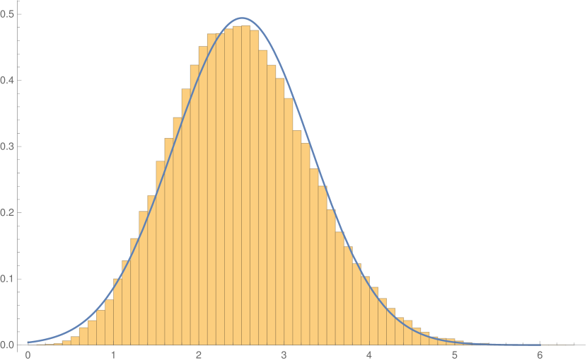
(a) $k=2$

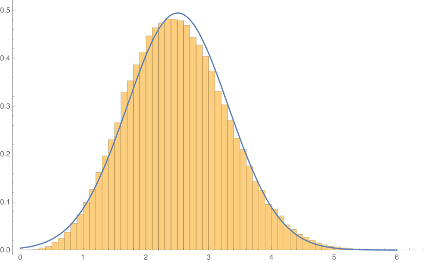
(b) $k=3$

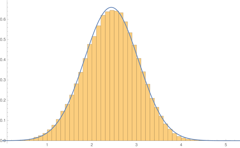
(c) $k=4$

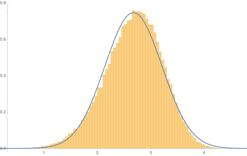
(d) $k=5$

Figure 3: Histograms of $10^{5}$ samples of ${\cal B}_{k}$ for $k=2,\dots,5$. The blue curves represent the density functions of ${\cal N}({\mathbf{E}}{\cal B}_{k},\sqrt{{\mathrm{Var}}\left({\cal B}_{k}\right)})$.

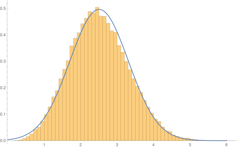
Figure 4: Simulation for ${\cal X}_{n}$ with $k=2$, $n=2^{17}$ and $60000$ samples, after rescaled by $\sqrt{n}$. The blue curve represents the density function of a normal distribution with the empirical mean and variance.

4 Some extensions

4.1 A lower bound and an upper bound for general graphs

Let ${\cal G}_{n}$ be the set of rooted graphs with $n$ nodes. It is obvious that $\mathbb{P}_{n}$ is the easiest to cut among all graphs in ${\cal G}_{n}$. We formalize this by the following lemma:

Lemma 10.

Let $k\in{\mathbb{N}}$. For all $\mathbb{G}_{n}\in{\cal G}_{n}$, ${\cal X}_{n}\,{\buildrel{\mathrm{def}}\over{=}}\,{\cal K}(\mathbb{P}_{n})\preceq{\cal K}(\mathbb{G}_{n}).$ Therefore,

$$\min_{\mathbb{G}_{n}\in{\cal G}_{n}}{\mathbf{E}}{{\cal K}(\mathbb{G}_{n})}\geq{\mathbf{E}}{{\cal X}_{n}}\sim\left\{\begin{array}[]{*2{>{\displaystyle}l}}\frac{(k!)^{\frac{1}{k}}}{k-1}\Gamma\left(\frac{1}{k}\right)n^{1-\frac{1}{k}}&(k\geq 2),\\ \log n&(k=1),\end{array}\right.$$ (4.1)

by Theorem 1.

The most resilient graph is obviously $\mathbb{K}_{n}$, the complete graph with $n$ vertices. Thus, we have the following upper bound:

Lemma 11.

Let $k\in{\mathbb{N}}$.

1. Let $Y\,{\buildrel{\cal L}\over{=}}\,\mathop{\mathrm{Gamma}}(k)$, $Z\,{\buildrel{\cal L}\over{=}}\,\mathop{\mathrm{Poi}}(Y)$, and $W\,{\buildrel{\cal L}\over{=}}\,Z\wedge k$, i.e., $W\,{\buildrel{\cal L}\over{=}}\,\min\{Z,k\}$. Then

   $${\cal L}\left(\frac{{\cal K}(\mathbb{K}_{n})}{n}\right){\,{\buildrel d\over{\rightarrow}}\,}{\cal L}\left({\mathbf{E}}\left[W|Y\right]\right)={\cal L}\left(\frac{\Gamma(k+1,Y)-e^{-Y}Y^{k+1}}{k!}+k\right),$$ (4.2)

   where $\Gamma(\ell,z)$ denotes the upper incomplete gamma function. Note that when $k=1$, the right-hand-side is simply $\mathop{\mathrm{Unif}}[0,1]$.

2. For all $\mathbb{G}_{n}\in{\cal G}_{n}$, ${\cal K}(\mathbb{G}_{n})\preceq{\cal K}(\mathbb{K}_{n}).$ Therefore,

   $$\max_{\mathbb{G}_{n}\in{\cal G}_{n}}{\mathbf{E}}{{\cal K}(\mathbb{G}_{n})}\leq{\mathbf{E}}{{\cal K}(\mathbb{K}_{n})}\sim k\left(1-\frac{1}{2^{2k}}\binom{2k}{k}\right)n.$$ (4.3)

Proof.

Let $S_{n}$ be the tree of $n$ nodes with one root and $n-1$ leaves. Obviously ${\cal K}(\mathbb{K}_{n})\,{\buildrel{\cal L}\over{=}}\,{\cal K}(S_{n})$. Let $Y$ be the time when the root is removed. Let $W_{1,n},\dots,W_{n-1,n}$ be the number of cuts each leaf receives by this time. Conditioning on the event $Y=y$, $W_{1,n},\dots,W_{n-1,n}$ are i.i.d. with $W_{i,n}\,{\buildrel{\cal L}\over{=}}\,Z_{i}\wedge k$, where $Z_{i}\,{\buildrel{\cal L}\over{=}}\,\mathop{\mathrm{Poi}}(y)$. In other words, conditioning on $Y=y$, by the law of large numbers,

$$\frac{{\cal K}(S_{n})}{n}=\frac{k+\sum_{i=1}^{n-1}W_{i,n}}{n}\,{\buildrel{a.s.}\over{\rightarrow}}\,{\mathbf{E}}\left[Z_{1}\right],$$ (4.4)

from which (4.2) and (4.3) follow immediately. ∎

4.2 Path-like graphs

If a graph $\mathbb{G}_{n}$ consists of only long paths, then the limit distribution ${\cal K}(\mathbb{G}_{n})$ should be related to ${\cal B}_{k}$, the limit distribution of ${\cal K}(\mathbb{P}_{n})/n^{1-\frac{1}{k}}$ (see Theorem 4). We give two simple examples with $k\in\{2,3,\dots\}$.

Example 1 (Long path).

Let $(\mathbb{G}_{n})_{n\geq 1}$ be a sequence of rooted graphs such that $\mathbb{G}_{n}$ contains a path of length $m(n)$ starting from the root with $n-m(n)=o(n^{1-\frac{1}{k}})$. Since it takes at most $k(n-m(n))$ cuts to remove all the nodes outside the long path,

$${\cal K}(P_{m(n)})\preceq{\cal K}(\mathbb{G}_{n})\preceq{\cal K}(P_{m(n)})+k{o\!\left(n^{1-1/k}\right)}.$$

Thus, by Lemma 10, this implies that ${\cal K}(\mathbb{G}_{n})/n^{1-\frac{1}{k}}$ converges in distribution to ${\cal B}_{k}$.

Example 2 (Curtain).

Let $\ell\geq 2$ be a fixed integer. Let $\mathbb{T}^{(\ell)}_{n}$ be a graph that consists of only $\ell$ paths connected to the root, with the first $\ell-1$ of them having length $\left\lceil\frac{n-1}{\ell}\right\rceil$. We call $\mathbb{T}^{(\ell)}_{n}$ an $\ell$-curtain. It is easy to see that cutting $\mathbb{T}^{(\ell)}_{n}$ is very similar to cutting $\ell$ separated paths of length $\left\lceil\frac{n}{\ell}\right\rceil$. Therefore, we can show that

$$\frac{{\cal K}(\mathbb{T}^{(\ell)}_{n})}{\left(n/\ell\right)^{\frac{1}{k}}}{\,{\buildrel d\over{\rightarrow}}\,}\sum_{j=1}^{\ell}{\cal B}_{k}^{[j]},$$ (4.5)

where ${\cal B}_{k}^{[1]},\dots,{\cal B}_{k}^{[\ell]}$ are i.i.d. copies of ${\cal B}_{k}$.

4.3 Deterministic and random trees

The approximation given in Lemma 1 can be used to compute the expectation of $k$-cut numbers in many deterministic or random trees. We give four examples: complete binary trees, split trees, random recursive trees, and Galton-Watson trees.

4.3.1 Complete binary trees

Let $\mathbb{T}^{\mathrm{bi}}_{n}$ be a complete binary tree of with $n=2^{m+1}-1$ nodes, i.e., its height is $m$. Recall that $I_{r,i+1}$ in Lemma 1 is the indicator that a node in $\mathbb{P}_{n}$ at depth $i$ is an $r$-record. Since the probability of a node being an $r$-record only depends on its depth, it follows from Lemma 1 that

$${\mathbf{E}}{{\cal K}_{r}(\mathbb{T}^{\mathrm{bi}}_{n})}=\sum_{i=0}^{m}2^{i}{\mathbf{E}}{I_{r,i+1}}\sim\frac{(k!)^{\frac{r}{k}}}{k}\frac{\Gamma\left(\frac{r}{k}\right)}{\Gamma(r)}\frac{2^{m+1}}{m^{\frac{r}{k}}}.$$ (4.6)

Thus, only the one-records matter as in the case of $\mathbb{P}_{n}$ and

$${\mathbf{E}}{{\cal K}(\mathbb{T}^{\mathrm{bi}}_{n})}\sim{\mathbf{E}}{{\cal K}_{1}(\mathbb{T}^{\mathrm{bi}}_{n})}\sim\frac{(k!)^{\frac{1}{k}}{\Gamma\left(\frac{1}{k}\right)}}{k}\frac{2^{m+1}}{m^{\frac{1}{k}}}\sim\frac{(k!)^{\frac{1}{k}}{\Gamma\left(\frac{1}{k}\right)}}{k}\frac{n}{\left(\log_{2}n\right)^{\frac{1}{k}}}.$$ (4.7)

The limit distribution of ${\cal K}(\mathbb{T}^{\mathrm{bi}}_{n})$ has been found in our follow-up paper [4].

4.3.2 Split trees

Split trees were first defined by [7] to encompass many families of trees that are frequently used in algorithm analysis, e.g., binary search trees and tries. Its exact construction is somewhat lengthy and we refer readers to either the original algorithmic definition in [14] or the more probabilistic version in [3, Section 2].

Very roughly speaking, $\mathbb{T}^{\mathrm{sp}}_{n}$ is constructed by first distributing randomly $n$ balls among the nodes of an infinite $b$-ary tree and then removing all subtrees without balls. Each node in the infinite $b$-ary tree is given a random non-negative split vector ${\cal V}=(V_{1},\dots,V_{b})$, satisfying $\sum_{i=1}^{b}V_{i}=1$, drawn independently from the same distribution. These vectors affect how balls are distributed.

In the study of split trees, the following condition of ${\cal V}$ is often assumed:

Condition A.

The split vector ${\cal V}$ is permutation invariant. Moreover, ${\mathbf{P}}\left\{V_{1}=1\right\}=0$, ${\mathbf{P}}\left\{V_{1}=0\right\}=0$, and that $-\log(V_{1})$ is non-lattice.

[14, Theorem 1.1 ] showed that , assuming condition A, there exists a constant $\alpha$ such that ${\mathbf{E}}N\sim\alpha n$, where $N$ is the random number of nodes in $\mathbb{T}^{\mathrm{sp}}_{n}$.

In the setup of split trees (and other random trees), we obtain ${\cal K}(\mathbb{T}^{\mathrm{sp}}_{n})$ by choosing a random split tree first and then carry out the $k$-cut process conditioning on the tree. [13, Theorem 1.1 ] showed that condition A implies that ${\cal K}_{k}(\mathbb{T}^{\mathrm{sp}}_{n})$ converges to a weakly $1$-stable distribution after normalization, and that ${\mathbf{E}}{\cal K}_{k}(\mathbb{T}^{\mathrm{sp}}_{n})\sim{\mu\alpha n}/{\log n}$, where $\mu\,{\buildrel{\mathrm{def}}\over{=}}\,b{\mathbf{E}}\left[-V_{1}\log V_{1}\right]$. We extend this result as follows:

Lemma 12.

Assuming condition A, we have

$${\mathbf{E}}\left[{\cal K}_{r}(\mathbb{T}^{\mathrm{sp}}_{n})\right]\sim\frac{(k!\mu)^{\frac{r}{k}}}{k}\frac{\Gamma\left(\frac{r}{k}\right)}{\Gamma(r)}\frac{\alpha n}{(\log n)^{\frac{r}{k}}}, (1\leq r\leq k),$$ (4.8)

$${\mathbf{E}}\left[{\cal K}(\mathbb{T}^{\mathrm{sp}}_{n})\right]\sim(k!\mu)^{\frac{1}{k}}\frac{\Gamma\left(\frac{1}{k}\right)}{k}\frac{\alpha n}{(\log n)^{\frac{1}{k}}}.$$ (4.9)

Proof.

We say a node $v$ is good if it has depth $d(v)$ where $\left|d(v)-\frac{1}{\mu}\log n\right|\leq\log^{0.6}n,$ otherwise we say it is bad. Let $\mathbb{B}^{\mathrm{sp}}_{n}$ be the number of bad nodes in $\mathbb{T}^{\mathrm{sp}}_{n}$. By [14][Theorem 1.2], ${\mathbf{E}}{\mathbb{B}^{\mathrm{sp}}_{n}}={O\!\left({n}/{(\log n)^{3}}\right)}.$ Thus, the number of $r$-records in bad nodes is negligible and it suffices to prove the lemma for good nodes. By Lemma 1 and the definition of good nodes, we have

$${\mathbf{E}}\left[{\cal K}(\mathbb{T}^{\mathrm{sp}}_{n})|\mathbb{T}^{\mathrm{sp}}_{n}\right]= (N-\mathbb{B}^{\mathrm{sp}}_{n})\frac{(k!)^{\frac{r}{k}}}{k}\frac{\Gamma\left(\frac{r}{k}\right)}{\Gamma(r)}\left[\frac{\log n}{\mu}+O(\log^{0.6}n)\right]^{-\frac{r}{k}}(1+O(\log^{-\frac{1}{2k}}n))$$

$$= (N-\mathbb{B}^{\mathrm{sp}}_{n})\frac{(k!\mu)^{\frac{r}{k}}}{k}\frac{\Gamma\left(\frac{r}{k}\right)}{\Gamma(r)}\frac{1}{\left(\log n\right)^{\frac{r}{k}}}(1+O(\log^{-\frac{1}{2k}}n)),$$

from which the lemma follows by taking expectation and using that ${\mathbf{E}}N\sim\alpha n$. ∎

4.3.3 Random recursive trees

A random recursive tree $\mathbb{T}^{\mathrm{rr}}_{n}$ is random tree of $n$ nodes constructed recursively as follows: let $\mathbb{T}^{\mathrm{rr}}_{1}$ be the tree of a single node labeled $1$; given $\mathbb{T}^{\mathrm{rr}}_{n-1}$, choose a node in $\mathbb{T}^{\mathrm{rr}}_{n-1}$ uniformly at random and attach a node labeled $n$ to the selected node as a child, which gives $\mathbb{T}^{\mathrm{rr}}_{n}$. [22] introduced this model and showed that ${\mathbf{E}}{\cal K}_{k}(\mathbb{T}^{\mathrm{rr}}_{n})\sim n/\log n$ and that ${\cal K}_{k}(\mathbb{T}^{\mathrm{rr}}_{n})$ concentrates around its mean. [9] and subsequently [15] proved ${\cal K}(\mathbb{T}^{\mathrm{rr}}_{n})$ converges weakly to a stable law after proper shifting and normalization.

The intuition behind ${\mathbf{E}}{\cal K}_{k}(\mathbb{T}^{\mathrm{rr}}_{n})\sim n/\log n$ is simply that almost all nodes in $\mathbb{T}^{\mathrm{rr}}_{n}$ are at depth around $\log n$. We say a node $v$ in $\mathbb{T}^{\mathrm{rr}}_{n}$ is good if $|d(v)-\log(n)|\leq\log(n)^{0.9}$; otherwise we say it is bad. The following lemma shows that there are very few bad nodes in expectation:

Lemma 13.

Let $\mathbb{B}^{\mathrm{rr}}_{n}$ be the number of bad nodes in $\mathbb{T}^{\mathrm{rr}}_{n}$, then ${\mathbf{E}}\mathbb{B}^{\mathrm{rr}}_{n}={O\!\left({n}/{\log(n)^{3}}\right)}$.

Proof.

Let $h(\mathbb{T}^{\mathrm{rr}}_{n})$ be the height of $\mathbb{T}^{\mathrm{rr}}_{n}$. By [8, 6.3.2]

$${\mathbf{P}}\left\{|h(\mathbb{T}^{\mathrm{rr}}_{n})-\mathrm{e}\log(n)|>\eta\right\}={O\!\left(\mathrm{e}^{-c\eta}\right)},$$ (4.10)

for some constant $c$. Thus, we can choose some constant $K$ large enough and ignore the nodes of depth greater than $K\log(n)$. Let $w_{d}(\mathbb{T}^{\mathrm{rr}}_{n})$ be the number of nodes at depth $d$ in $\mathbb{T}^{\mathrm{rr}}_{n}$. By [11, Equation 3]

$${\mathbf{E}}\left[w_{d}(\mathbb{T}^{\mathrm{rr}}_{n})\right]=\frac{\log(n)^{d}}{\Gamma(1+d/\log(n))d!}\left(1+{O\!\left(\log(n)^{-1}\right)}\right),$$ (4.11)

uniformly for all $n\geq 3$ and $1\leq d\leq K\log(n)$, for all $K\geq 1$. Thus, the lemma follows by summing both sides of (4.11) over integers $d$ in $[1,\log(n)-\log(n)^{0.9}]\cup[\log(n)+\log(n)^{0.9},K\log(n)].$ ∎

Thus, by exactly the same argument of Lemma 12, we get:

Lemma 14.

We have

$${\mathbf{E}}\left[{\cal K}_{r}(\mathbb{T}^{\mathrm{rr}}_{n})\right]\sim\frac{(k!)^{\frac{r}{k}}}{k}\frac{\Gamma\left(\frac{r}{k}\right)}{\Gamma(r)}\frac{n}{(\log n)^{\frac{r}{k}}}, (1\leq r\leq k),$$ (4.12)

$${\mathbf{E}}\left[{\cal K}(\mathbb{T}^{\mathrm{rr}}_{n})\right]\sim(k!)^{\frac{1}{k}}\frac{\Gamma\left(\frac{1}{k}\right)}{k}\frac{n}{(\log n)^{\frac{1}{k}}}.$$ (4.13)

Remark 4.

We have not tried to find the limit distributions for ${\cal K}(\mathbb{T}^{\mathrm{sp}}_{n})$, and ${\cal K}(\mathbb{T}^{\mathrm{rr}}_{n})$. But $\mathbb{T}^{\mathrm{sp}}_{n}$ and $\mathbb{T}^{\mathrm{rr}}_{n}$ are both of logarithmic height. Thus, the same method which we used for treating complete binary trees [4] should also work.

4.3.4 Conditional Galton-Watson trees

A Galton-Watson tree $\mathbb{T}^{\mathrm{gw}}$ is a random tree that starts with the root node and recursively attaches a random number of children to each node in the tree, where the numbers of children are drawn independently from the same distribution ${\cal L}(\xi)$ (the offspring distribution). A conditional Galton-Watson tree $\mathbb{T}^{\mathrm{gw}}_{n}$ is $\mathbb{T}^{\mathrm{gw}}$ restricted to size $n$. See [18] for a comprehensive survey of conditional Galton-Watson trees.

[17, Theorem 1.6 ] showed that ${{\cal K}_{k}(\mathbb{T}^{\mathrm{gw}}_{n})}/\sqrt{n}$ converges weakly to a Rayleigh distribution and the convergence is also in all moments if $\xi$ has a finite exponential moment. In particular

$$\frac{{\mathbf{E}}{{\cal K}_{k}(\mathbb{T}^{\mathrm{gw}}_{n})}}{\sqrt{n}}\to{\mathbf{E}}\left[\int_{0}^{1}\left(\frac{2e(t)}{\sigma}\right)^{-1}\mathrm{d}t\right]=\sigma\sqrt{\frac{\pi}{2}},$$ (4.14)

where $e(t)$ denotes a normalized Brownian excursion and $\sigma^{2}={\mathrm{Var}}\left(\xi\right)$. It is straight forward to adapt the method in [17] to get the first moment of ${\mathbf{E}}{{\cal K}_{r}(\mathbb{T}^{\mathrm{gw}}_{n})}$. (Though higher moments and the limit distribution seems to be elusive.) We formulate this as lemma and refer the reader to [17] for details.

Lemma 15.

Assume that ${\mathbf{E}}\left[\xi^{3}\right]<\infty$. Then for $r\in\{1,\dots,k\}$,

$$\frac{{\mathbf{E}}{{\cal K}_{r}(\mathbb{T}^{\mathrm{gw}}_{n})}}{n^{1-\frac{r}{2k}}}\to\frac{(k!)^{\frac{r}{k}}}{k}\frac{\Gamma(\frac{r}{k})}{\Gamma(r)}{\mathbf{E}}\left[\int_{0}^{1}\left(\frac{2e(t)}{\sigma}\right)^{-\frac{r}{k}}\mathrm{d}t\right]=\frac{(k!)^{\frac{r}{k}}}{k}\frac{\Gamma(\frac{r}{k})\Gamma\left(1-\frac{r}{2k}\right)}{\Gamma(r)}\left(\frac{\sigma}{\sqrt{2}}\right)^{\frac{r}{k}}.$$ (4.15)

As a result,

$${\mathbf{E}}{{\cal K}(\mathbb{T}^{\mathrm{gw}}_{n})}\sim{\mathbf{E}}{{\cal K}_{1}(\mathbb{T}^{\mathrm{gw}}_{n})}\sim\frac{(k!)^{\frac{1}{k}}}{k}{\Gamma\left(\frac{1}{k}\right)\Gamma\left(1-\frac{1}{2k}\right)}\left(\frac{\sigma}{\sqrt{2}}\right)^{\frac{1}{k}}n^{1-\frac{1}{2k}}.$$ (4.16)

5 Some auxiliary results

Lemma 16.

Let $G_{k}\,{\buildrel{\cal L}\over{=}}\,\mathop{\mathrm{Gamma}}(k)$. Let $\alpha\,{\buildrel{\mathrm{def}}\over{=}}\,\frac{1}{2}\left(\frac{1}{k}+\frac{1}{k+1}\right)$ and $x_{0}\,{\buildrel{\mathrm{def}}\over{=}}\,m^{-\alpha}$. Then uniformly for all $x\in[0,x_{0}]$,

$${\mathbf{P}}\left\{G_{k}>x\right\}^{m}=\left(\frac{\Gamma\left(k,x\right)}{\Gamma(k)}\right)^{m}=\left(1+{O\!\left(m^{-\frac{1}{2k}}\right)}\right)\exp\left(-\frac{mx^{k}}{k!}\right),$$ (5.1)

where $\Gamma(\ell,z)$ denotes the upper incomplete gamma function.

Proof.

By the density function of gamma distributions, ${\mathbf{P}}\left\{G_{k}>x\right\}={\Gamma\left(k,x\right)}/{\Gamma(k)}.$ It then follows from the series expansion of the incomplete gamma function [24, 8.7.3], that uniformly for all $x\leq x_{0}$,

$$\left(\frac{\Gamma\left(k,x\right)}{\Gamma(k)}\right)^{m}=\left(1-\frac{x^{k}}{k!}+{O\!\left(x_{0}^{k+1}\right)}\right)^{m}=\left(1+{O\!\left(m^{-\frac{1}{2k}}\right)}\right)\exp\left(-\frac{mx^{k}}{k!}\right),$$ (5.2)

where we use that $-\alpha(k+1)+1=-\frac{1}{2k}$. ∎

Lemma 17.

Let $G_{k}\,{\buildrel{\cal L}\over{=}}\,\mathop{\mathrm{Gamma}}(k)$. Let $a\geq 0$ and $b\geq 1$ be fixed. Then uniformly for $m\geq 1$,

$$\int_{0}^{\infty}x^{b-1}{\mathrm{e}}^{-ax}{\mathbf{P}}\left\{G_{k}>x\right\}^{m}\,\mathrm{d}x=\left(1+{O\!\left(m^{-\frac{1}{2k}}\right)}\right)\frac{(k!)^{\frac{b}{k}}}{k}{\Gamma\left(\frac{b}{k}\right)}m^{-\frac{b}{k}}.$$ (5.3)

Proof.

By Lemma 16, the left-hand-side of (5.3) equals

$$\int_{0}^{x_{0}}{x^{b-1}{\mathrm{e}}^{-ax}}\left(\frac{\Gamma\left(k,x\right)}{\Gamma(k)}\right)^{m}\,\mathrm{d}x+\int_{x_{0}}^{\infty}{x^{b-1}{\mathrm{e}}^{-ax}}\left(\frac{\Gamma\left(k,x\right)}{\Gamma(k)}\right)^{m}\,\mathrm{d}x\,{\buildrel{\mathrm{def}}\over{=}}\,A_{1}+A_{2},$$ (5.4)

where $x_{0}=m^{-\alpha}$ and $\alpha=\frac{1}{2}\left(\frac{1}{k}+\frac{1}{k+1}\right)$. Then

$$A_{1} =\left(1+{O\!\left(m^{-\frac{1}{2k}}\right)}\right)\int_{0}^{x_{0}}{x^{b-1}{\mathrm{e}}^{-ax}}\exp\left(-\frac{mx^{k}}{k!}\right)\,\mathrm{d}x$$ (5.5)

$$=\left(1+{O\!\left(m^{-\frac{1}{2k}}\right)}\right)\frac{(k!)^{\frac{b}{k}}}{k}\left(\Gamma\left(\frac{b}{k}\right)-\Gamma\left(\frac{b}{k},w_{0}\right)\right)m^{-\frac{b}{k}},$$ (5.6)

where $w_{0}=\frac{mx_{0}^{k}}{k!}=\Theta(m^{\frac{1}{2k(k+1)}})$. By the upper bound given in [24, 8.11.i], $\Gamma\left(\frac{b}{k},w_{0}\right)={O\!\left({\mathrm{e}}^{-\frac{w_{0}}{2}}\right)}$, which is exponentially small and can be neglected. Using (5.2), one can verify that $A_{2}={O\!\left({\mathrm{e}}^{-\frac{w_{0}}{2}}\right)}$ which can also be neglected. ∎

Lemma 18.

For $a>0$, $b>0$ and $k\geq 2$,

$$\xi_{k}(a,b) \,{\buildrel{\mathrm{def}}\over{=}}\,\int_{0}^{\infty}\int_{y}^{\infty}\mathrm{e}^{-ax^{k}/k!-by^{k}/k!}\,\mathrm{d}x\,\mathrm{d}y$$ (5.7)

$$=\frac{\Gamma\left(\frac{2}{k}\right)}{k}\left(\frac{k!}{a}\right)^{\frac{2}{k}}F\left(\frac{2}{k},\frac{1}{k};1+\frac{1}{k};-\frac{b}{a}\right),$$ (5.8)

where $F$ denotes the hypergeometric function. In particular,

$$\xi_{2}(a,b)={\arctan\left(\sqrt{\frac{b}{a}}\right)}{(ab)^{-\frac{1}{2}}}.$$ (5.9)

Proof.

Changing to polar system by $x=r\cos(\theta)$ and $y=r\sin(\theta)$,

$$\xi_{k}(a,b)= \int_{0}^{\pi/4}\int_{0}^{\infty}\exp\left[-r^{k}\left(a\frac{\cos(\theta)^{k}}{k!}+b\frac{\sin(\theta)^{k}}{k!}\right)\right]r\,\mathrm{d}r\,\mathrm{d}\theta$$ (5.10)

$$=\int_{0}^{\pi/4}\left(a\frac{\cos(\theta)^{k}}{k!}+b\frac{\sin(\theta)^{k}}{k!}\right)^{-\frac{2}{k}}\frac{\Gamma(\frac{2}{k})}{k}\,\mathrm{d}\theta$$ (5.11)

$$=\frac{\Gamma(\frac{2}{k})}{k}\left(\frac{k!}{a}\right)^{\frac{2}{k}}\int_{0}^{\pi/4}\left(1+\frac{b}{a}\tan(\theta)^{k}\right)^{-\frac{2}{k}}\,\mathrm{d}\theta$$ (5.12)

$$=\frac{\Gamma(\frac{2}{k})}{k^{2}}\left(\frac{k!}{a}\right)^{\frac{2}{k}}\int_{0}^{1}u^{\frac{1}{k}-1}\left(1+\frac{b}{a}u\right)^{-\frac{2}{k}}\,\mathrm{d}u,$$ (5.13)

which equals the right-hand-side of (5.8) by [24, 15.6.1]. For (5.9), see [24, 15.4.3]. ∎

Lemma 19.

For $a>0$, $b>0$ and $k\geq 2$,

$$(a+b)^{-\frac{2}{k}}\leq\frac{k}{\Gamma\left(\frac{2}{k}\right)\left(k!\right)^{\frac{2}{k}}}\xi_{k}(a,b)\leq a^{-\frac{2}{k}}+b^{-\frac{2}{k}}.$$ (5.14)

Moreover, $\xi_{k}(a,b)$ is monotonically decreasing in both $a$ and $b$.

Proof.

Let

$$\xi_{k}^{*}(a,b)\,{\buildrel{\mathrm{def}}\over{=}}\,\frac{k}{\Gamma\left(\frac{2}{k}\right)\left(k!\right)^{\frac{2}{k}}}\xi_{k}(a,b)=\left(a+b\right)^{-\frac{2}{k}}F\left(\frac{2}{k},1;1+\frac{1}{k};\frac{b}{a+b}\right),$$ (5.15)

where we use [24, 15.8.1]. Let $\alpha_{1}=\frac{k}{k+1}$. By [20, cor. 2 ], for $x\in(0,1)$,

$$\left(1-\alpha_{1}x\right)^{-\frac{2}{k}}\leq F\left(\frac{2}{k},1;1+\frac{1}{k};x\right)\leq 1-\alpha_{1}+\alpha_{1}\left(1-x\right)^{-\frac{2}{k}}.$$ (5.16)

This together with (5.15) give us (5.14).

For monotonicity, using the derivative formula [24, 15.5.1], it is easy to verify that for $a>0$ and $b>0$ $\frac{\partial}{\partial a}\xi_{k}^{*}(a,b)<0$ and $\frac{\partial}{\partial b}\xi_{k}^{*}(a,b)<0.$ ∎

Lemma 20.

For $k\geq 2$, let

$$\lambda_{k}\,{\buildrel{\mathrm{def}}\over{=}}\,\int_{0}^{1}\int_{0}^{1-s}\xi_{k}(s,t)\,\mathrm{d}t\,\mathrm{d}s.$$ (5.17)

Then

$$\lambda_{k}=\left\{\begin{array}[]{*2{>{\displaystyle}l}}\frac{\pi\cot\left(\frac{\pi}{k}\right)\Gamma\left(\frac{2}{k}\right)(k!)^{\frac{2}{k}}}{2\left({k}-2\right)\left({k}-1\right)}&k>2,\\ \frac{\pi^{2}}{4}&k=2.\end{array}\right.$$ (5.20)

Proof.

When $k=2$, applying (5.9) and changing to the polar system by letting $s=(r\cot(\theta))^{2}$ and $t=(r\sin(\theta))^{2}$, we get

$$\lambda_{2}=\int_{0}^{1}\int_{0}^{1-s}\frac{\arctan\left(\sqrt{\frac{t}{s}}\right)}{\sqrt{st}}=\int_{0}^{\frac{\pi}{2}}\int_{0}^{1}4r\theta\,\mathrm{d}r\,\mathrm{d}\theta=\frac{\pi^{2}}{4}.$$ (5.21)

For $k\geq 3$, by Lemma 18, it suffices to show that

$$\int_{0}^{1}s^{-\frac{2}{k}}\int_{0}^{1-s}F\left(\frac{2}{k},\frac{1}{k};1+\frac{1}{k};-\frac{t}{s}\right)\,\mathrm{d}t\,\mathrm{d}s=\frac{k\pi\cot\left(\frac{\pi}{k}\right)}{2(k-2)(k-1)},$$ (5.22)

which is easily verifiable using Mathematica. A human proof can be derived using the series expansion of hypergeometric function [24, 15.6.1]. ∎

Remark 5.

In an attempt to prove Lemma 20, we discovered the following identity

$$\int_{0}^{\infty}(w+1)^{\frac{2}{k}-2}\,F\left(\frac{2}{k},\frac{1}{k};1+\frac{1}{k};-w\right)\,\mathrm{d}w=\frac{\pi\cot\left(\frac{\pi}{k}\right)}{k-2}, \left(k\geq 3\right),$$ (5.23)

which we have not found in the literature. The proof follows from changing to polar system in the left-hand-side of (5.22) by letting $s=(r\cos(\theta))^{k}$ and $t=(r\sin(\theta))^{k}$.

References

- [1] Louigi Addario-Berry, Nicolas Broutin and Cecilia Holmgren “Cutting down trees with a Markov chainsaw” In Ann. Appl. Probab. 24.6, 2014, pp. 2297–2339 URL: https://doi.org/10.1214/13-AAP978
- [2] M. Ahsanullah “Record Values–Theory and Applications” University Press of America, Inc., Lanham, MD, 2004
- [3] Xing Shi Cai, C. Holmgren, S. Janson, T. Johansson and F. Skerman “Inversions in Split Trees and Conditional Galton–Watson Trees” Published online In Combinatorics, Probability and Computing Cambridge University Press, 2018 DOI: 10.1017/S0963548318000512
- [4] Xing Shi Cai and Cecilia Holmgren “Cutting resilient networks – complete binary trees” In arXiv e-prints, 2018 arXiv:1811.05673 [math.PR]
- [5] K.. Chandler “The distribution and frequency of record values” In J. Roy. Statist. Soc. Ser. B. 14, 1952, pp. 220–228 URL: http://links.jstor.org/sici?sici=0035-9246(1952)14:2%3C220:TDAFOR%3E2.0.CO;2-D&origin=MSN
- [6] D. Dagon, G. Gu, C.. Lee and W. Lee “A Taxonomy of Botnet Structures” In Twenty-Third Annual Computer Security Applications Conference (ACSAC 2007), 2007, pp. 325–339 DOI: 10.1109/ACSAC.2007.44
- [7] Luc Devroye “Universal limit laws for depths in random trees” In SIAM J. Comput. 28.2, 1999, pp. 409–432 DOI: 10.1137/S0097539795283954
- [8] Michael Drmota “Random Trees: An Interplay between Combinatorics and Probability” Wien: Springer-Verlag, 2009 URL: //www.springer.com/gp/book/9783211753552
- [9] Michael Drmota, Alex Iksanov, Martin Moehle and Uwe Roesler “A limiting distribution for the number of cuts needed to isolate the root of a random recursive tree” In Random Structures Algorithms 34.3, 2009, pp. 319–336 URL: https://doi.org/10.1002/rsa.20233
- [10] Rick Durrett “Probability: Theory and Examples” 31, Cambridge Series in Statistical and Probabilistic Mathematics Cambridge University Press, Cambridge, 2010 DOI: 10.1017/CBO9780511779398
- [11] Michael Fuchs, Hsien-Kuei Hwang and Ralph Neininger “Profiles of random trees: limit theorems for random recursive trees and binary search trees” In Algorithmica 46.3-4, 2006, pp. 367–407 DOI: 10.1007/s00453-006-0109-5
- [12] Cecilia Holmgren “Random records and cuttings in binary search trees” In Combin. Probab. Comput. 19.3, 2010, pp. 391–424 URL: https://doi.org/10.1017/S096354830999068X
- [13] Cecilia Holmgren “A weakly 1-stable distribution for the number of random records and cuttings in split trees” In Adv. in Appl. Probab. 43.1, 2011, pp. 151–177 URL: https://doi.org/10.1239/aap/1300198517
- [14] Cecilia Holmgren “Novel characteristic of split trees by use of renewal theory” In Electron. J. Probab. 17, 2012, pp. no. 5\bibrangessep27 DOI: 10.1214/EJP.v17-1723
- [15] Alex Iksanov and Martin Möhle “A probabilistic proof of a weak limit law for the number of cuts needed to isolate the root of a random recursive tree” In Electron. Comm. Probab. 12, 2007, pp. 28–35 URL: https://doi.org/10.1214/ECP.v12-1253
- [16] Svante Janson “Random records and cuttings in complete binary trees” In Mathematics and Computer Science. III, Trends Math. Birkhäuser, Basel, 2004, pp. 241–253
- [17] Svante Janson “Random cutting and records in deterministic and random trees” In Random Structures Algorithms 29.2, 2006, pp. 139–179 URL: https://doi.org/10.1002/rsa.20086
- [18] Svante Janson “Simply generated trees, conditioned Galton-Watson trees, random allocations and condensation” In Probab. Surv. 9, 2012, pp. 103–252 URL: https://doi.org/10.1214/11-PS188
- [19] Norman L. Johnson, Samuel Kotz and N. Balakrishnan “Continuous Univariate Distributions. Vol. 1” A Wiley-Interscience Publication, Wiley Series in Probability and Mathematical Statistics: Applied Probability and Statistics John Wiley & Sons, Inc., New York, 1994
- [20] D.. Karp “Representations and inequalities for generalized hypergeometric functions” In J. Math. Sci. (N.Y.) 207.6, 2015, pp. 885–897 DOI: 10.1007/s10958-015-2412-7
- [21] A. Meir and J.. Moon “Cutting down random trees” In J. Austral. Math. Soc. 11, 1970, pp. 313–324
- [22] A. Meir and J.W. Moon “Cutting down recursive trees” In Mathematical Biosciences 21.3, 1974, pp. 173–181 DOI: 10.1016/0025-5564(74)90013-3
- [23] Michael Molloy and Bruce Reed “Graph Colouring and the Probabilistic Method” 23, Algorithms and Combinatorics Springer-Verlag, Berlin, 2002, pp. xiv+326 URL: https://doi.org/10.1007/978-3-642-04016-0
- [24] “NIST Handbook of Mathematical Functions” U.S. Department of Commerce, National Institute of StandardsTechnology, Washington, DC; Cambridge University Press, Cambridge, 2010
- [25] Alfréd Rényi “Théorie des éléments saillants d’une suite d’observations” In Ann. Fac. Sci. Univ. Clermont-Ferrand No. 8, 1962, pp. 7–13