Geometry and the Imagination in Minneapolis

Abstract

This document consists of the collection of handouts for a two-week summer workshop entitled ’Geometry and the Imagination’, led by John Conway, Peter Doyle, Jane Gilman and Bill Thurston at the Geometry Center in Minneapolis, June 17-28, 1991. The workshop was based on a course ‘Geometry and the Imagination’ which we had taught twice before at Princeton.

1 Preface

This document consists of the collection of handouts for a two-week summer workshop entitled ’Geometry and the Imagination’, led by John Conway, Peter Doyle, Jane Gilman and Bill Thurston at the Geometry Center in Minneapolis, June 17-28, 1991. The workshop was based on a course ‘Geometry and the Imagination’ which we had taught twice before at Princeton.

The handouts do not give a uniform treatment of the topics covered in the workshop: some ideas were treated almost entirely in class by lecture and discussion, and other ideas which are fairly extensively documented were only lightly treated in class. The motivation for the handouts was mainly to supplement the class, not to document it.

The primary outside reading was ‘The Shape of Space’, by Jeff Weeks. Some of the topics discussed in the course which are omitted or only lightly covered in the handouts are developed well in that book: in particular, the concepts of extrinsic versus intrinsic topology and geometry, and two and three dimensional manifolds. Our approach to curvature is only partly documented in the handouts. Activities with scissors, cabbage, kale, flashlights, polydrons, sewing, and polyhedra were really live rather than written.

The mix of students—high school students, college undergraduates, high school teachers and college teachers—was unusual, and the mode of running a class with the four of us teaching was also unusual. The mixture of people helped create the tremendous flow of energy and enthusiasm during the workshop.

Besides the four teachers and the official students, there were many people who put a lot in to help organize or operate the course, including Jennifer Alsted, Phil Carlson, Anthony Iano-Fletcher, Maria Iano-Fletcher, Kathy Gilder, Harvey Keynes, Al Marden, Delle Maxwell, Jeff Ondich, Tony Phillips, John Sullivan, Margaret Thurston, Angie Vail, Stan Wagon.

2 Philosophy

Welcome to Geometry and the Imagination!

This course aims to convey the richness, diversity, connectedness, depth and pleasure of mathematics. The title is taken from the classic book by Hilbert and Cohn-Vossen, “Geometry and the Imagination’. Geometry is taken in a broad sense, as used by mathematicians, to include such fields as topology and differential geometry as well as more classical geometry. Imagination, an essential part of mathematics, means not only the facility which is imaginative, but also the facility which calls to mind and manipulates mental images. One aim of the course is to develop the imagination.

While the mathematical content of the course will be high, we will try to make it as independent of prior background as possible. Calculus, for example, is not a prerequisite.

We will emphasize the process of thinking about mathematics. Assignments will involve thinking and writing, not just grinding through formulas. There will be a strong emphasis on projects and discussions rather than lectures. All students are expected to get involved in discussions, within class and without. A Geometry Room on the fifth floor will be reserved for students in the course. The room will accrete mathematical models, materials for building models, references related to geometry, questions, responses and (most important) people. There will be computer workstations in or near the geometry room. You are encouraged to spend your afternoons on the fifth floor.

The spirit of mathematics is not captured by spending 3 hours solving 20 look-alike homework problems. Mathematics is thinking, comparing, analyzing, inventing, and understanding. The main point is not quantity or speed—the main point is quality of thought. The goal is to reach a more complete and a better understanding. We will use materials such as mirrors, Polydrons, scissors and tissue paper not because we think this is easier than solving algebraic equations and differential equations, but because we think that this is the way to bring thinking and reasoning to the course.

We are very enthusiastic about this course, and we have many plans to facilitate your taking charge and learning. While you won’t need a heavy formal background for the course, you do need a commitment of time and energy.

3 Organization

3.1 People

We are experimenting with a diverse group of participants in this course: high school students, high school teachers, college students, college teachers, and others.

Topics in mathematics often have many levels of meaning, and we hope and expect that despite—no, because of—the diversity, there will be a lot for everyone (including we the staff) to get from the course. As you think about something, you come to understand it from different angles, and on successively deeper levels.

We want to encourage interactions between all the participants in the course. It can be quite interesting for people with sophisticated backgrounds and with elementary backgrounds to discuss a topic with each other, and the communication can have a high value in both directions.

3.2 Scheduled meetings

The officially scheduled morning sessions, which run from 9:00 to 12:30 with a half-hour break in the middle, form the core of the course. During these sessions, various kinds of activities will take place. There will be some more-or-less traditional presentations, but the main emphasis will be on encouraging you to discover things for yourself. Thus the class will frequently break into small groups of about 5–7 people for discussions of various topics.

3.3 Discussion groups

We want to enable everyone to be engaged in discussions while at the same time preserving the unity of the course. From time to time, we will break into discussion groups of 5–7 people.

Every member of each group is expected to take part in the discussion and to make sure that everyone is involved: that everyone is being heard, everyone is listening, that the discussion is not dominated by one or two people, that everyone understands what is going on, and that the group sticks to the subject and really digs in.

Each group will have a reporter. The reporters will rotate so that everyone will serve as reporter during the next two weeks. The main role of the reporters during group discussions is to listen, rather than speak. The reporters should make sure they understand and write down the key points and ideas from the discussion, and be prepared to summarize and explain them to the whole class.

After a suitable time, we will ask for reports to the entire class. These will not be formal reports. Rather, we will hold a summary discussion among the reporters and teachers, with occasional contributions from others.

3.4 Texts

The required texts for the course are: Weeks, The Shape of Space and Coxeter, Introduction to Geometry. There are available at the University Bookstore.

Coxeter’s book will mainly be used as a reference book for the course, but it is also a book that should be useful to you in the future.

Here is a list of reading assignments from The Shape of Space by Weeks. As Weeks suggests it is important to “…read slowly and give things plenty of time to digest”, as much as is possible in a condensed course of this type.

• Monday, June 17: Chapters 1 and 2.

• Tuesday, June 18: Chapter 3.

• Wednesday, June 19: Chapter 4.

• Thursday, June 20: Chapter 5, pages 67-77, and Chapter 6, 85-90.

• Friday, June 21 – Sunday, June 23: Chapters 7 & 8.

• Monday, June 24: Chapters 9 and 10.

• Tuesday, June 25: Chapter 11 and 12.

• Wednesday, June 26: Chapter 13.

• Thursday, June 27: Chapter 16.

In addition, there is a long list of recommended reading. The geometry room has a small collection of additional books, which you may read there. There are several copies of some books which we highly recommend such as Flatland by Abbott and What is Mathematics by Courant and Robbins. There are single copies of other books.

3.5 Other materials

We will be doing a lot of constructions during class. Beginning this Tuesday (June 18th), you should bring with you to class each time: scissors, tape, ruler, compass, sharp pencils, plain white paper. It would be a capital idea to bring extras to rent to your classmates.

3.6 Journals

Each participant should keep a journal for the course. While assignments given at class meetings go in the journal, the journal is for much more: for independent questions, ideas, and projects. The journal is not for class notes, but for work outside of class. The style of the journal will vary from person to person. Some will find it useful to write short summaries of what went on in class. Any questions suggested by the class work should be in the journal. The questions can be either speculative questions or more technical questions. You may also want to write about the nature of the class meetings and group discussions: what works for you and what doesn’t work, etc.

You are encouraged to cooperate with each other in working on anything in the course, but what you put in your journal should be you. If it is something that has emerged from work with other people, write down who you have worked with. Ideas that come from other people should be given proper attribution. If you have referred to sources other than the texts for the course, cite them.

Exposition is important. If you are presenting the solution to a problem, explain what the problem is. If you are giving an argument, explain what the point is before you launch into it. What you should aim for is something that could communicate to a friend or a colleague a coherent idea of what you have been thinking and doing in the course.

Your journal should be kept on loose leaf paper. Journals will be collected every few days and read and commented upon by the instructors. If they are on loose leaf paper, you can hand in those parts which have not yet been read, and continue to work on further entries. Pages should be numbered consecutively and except when otherwise instructed, you should hand in only those pages which have not previously been read. Write your name on each page, and, in the upper right hand corner of the first page you hand in each time, list the pages you have handed in (e.g. [7,12] on page 7 will indicate that you have handed in 6 pages numbered seven to twelve).

Mainly, the journal is for you. In addition, the journals are an important tool by which we keep in touch with you and what you are thinking about. Our experience is that it is really fun and enjoyable when someone lets us into their head. No matter what your status in this course, keep a journal.

Journals will be collected and read as follows:

• Wed. June 19th

• Friday June 21st

• Tuesday, June 25th

• Thursday June 26th

Your entire journal should be handed in on Friday June 27th with your final project. We will return final journals by mail.

3.7 Constructions

Geometry lends itself to constructions and models, and we will expect everyone to be engaged in model-making. There will be minor constructions that may take only half an hour and that everyone does, but we will also expect larger constructions that may take longer.

3.8 Final project

We will not have a final exam for the course, but in its place, you will undertake a major project. The major project may be a paper investigating more deeply some topic we touch on lightly in class. Alternatively, it might be based on a major model project, or it might be a computer-based project. To give you some ideas, a list of possible projects will be circulated. However, you are also encouraged to come up with your own ideas for projects. If possible, your project should have some visual component, for we will display all of the projects at the end of the course at the Geometry Fair. The project will be due on the morning of Friday June 28th. The fair will be in the afternoon.

3.9 Geometry room/area

The fifth floor houses the Geometry Room. We hope that it will actually spill out into the hallways and corridors and thus become the geometry area. Thus the fifth floor will serve as a work and play room for this course. This is where you can find mathematical toys, games, models, displays and construction materials. Copies of handouts and books and other written materials of interest to students in the course will be kept here as well. It should also serve as a place to go if you want to talk to other students in the course, or to one of the teachers. Our current plan is to have this area open from 1:30 to 4:00 PM Monday through Friday, beginning right away. There will be a tour of the area at the end of Monday’s morning session.

4 Bicycle tracks

Here is a passage from a Sherlock Holmes story, The Adventure of the Priory School (by Arthur Conan Doyle):

‘This track, as you perceive, was made by a rider who was going from the direction of the school.’

‘Or towards it?’

‘No, no, my dear Watson. The more deeply sunk impression is, of course, the hind wheel, upon which the weight rests. You perceive several places where it has passed across and obliterated the more shallow mark of the front one. It was undoubtedly heading away from the school.’

1. Discuss the passage above.

2. Visualize, discuss, and sketch what bicycle tracks look like.

3. When we present actual bicycle tracks, determine the direction of motion.

4. What else can you tell about the bike from the tracks?

5 Polyhedra

A polyhedron is the three-dimensional version of a polygon: it is a chunk of space with flat walls. In other words, it is a three-dimensional figure made by gluing polygons together. The word is Greek in origin, meaning many-seated. The plural is polyhedra. The polygonal sides of a polyhedron are called its faces.

5.1 Discussion

Collect some triangles, either the snap-together plastic polydrons or paper triangles. Try gluing them together in various ways to form polyhedra.

1. Fasten three triangles together at a vertex. Complete the figure by adding one more triangle. Notice how there are three triangles at every vertex. This figure is called a tetrahedron because it has four faces (see the table of Greek number prefixes.)

2. Fasten triangles together so there are four at every vertex. How many faces does it have? From the table of prefixes below, deduce its name.

3. Do the same, with five at each vertex.

4. What happens when you fasten triangles six per vertex?

5. What happens when you fasten triangles seven per vertex?

1	mono
2	di
3	tri
4	tetra
5	penta
6	hexa
7	hepta
8	octa
9	ennia
10	deca
11	hendeca
12	dodeca
13	triskaideca
14	tetrakaideca
15	pentakaideca
16	hexakaideca
17	heptakaideca
18	octakaideca
19	enniakaideca
20	icosa

Table 1: The first 20 Greek number prefixes

5.2 Homework

A regular polygon is a polygon with all its edges equal and all angles equal. A regular polyhedron is one whose faces are regular polygons, all congruent, and having the same number of polygons at each vertex.

For homework, construct models of all possible regular polyhedra, by trying what happens when you fasten together regular polygons with 3, 4, 5, 6, 7, etc sides so the same number come together at each vertex.

Make a table listing the number of faces, vertices, and edges of each.

What should they be called?

6 Knots

A mathematical knot is a knotted loop. For example, you might take an extension cord from a drawer and plug one end into the other: this makes a mathematical knot.

It might or might not be possible to unknot it without unplugging the cord. A knot which can be unknotted is called an unknot.

Two knots are considered equivalent if it is possible to rearrange one to the form of the other, without cutting the loop and without allowing it to pass through itself. The reason for using loops of string in the mathematical definition is that knots in a length of string can always be undone by pulling the ends through, so any two lengths of string are equivalent in this sense.

If you drop a knotted loop of string on a table, it crosses over itself in a certain number of places. Possibly, there are ways to rearrange it with fewer crossings—the minimum possible number of crossings is the crossing number of the knot.

Figure 1: This is drawing of a knot has 7 crossings. Is it possible to rearrange it to have fewer crossings?

6.1 Discussion

Make drawings and use short lengths of string to investigate simple knots:

1. Are there any knots with one or two crossings? Why?

2. How many inequivalent knots are there with three crossings?

3. How many knots are there with four crossings?

4. How many knots can you find with five crossings?

5. How many knots can you find with six crossings?

7 Maps

A map in the plane is a collection of vertices and edges (possibly curved) joining the vertices such that if you cut along the edges the plane falls apart into polygons. These polygons are called the faces. A map on the sphere or any other surface is defined similarly. Two maps are considered to be the same if you can get from one to the other by a continouous motion of the whole plane. Thus the two maps in figure 2 are considered to be the same.

Figure 2: These two maps are considered the same (topologically equivalent), because it is possible to continuously move one to obtain the other.

A map on the sphere can be represented by a map in the plane by removing a point from the sphere and then stretching the rest of the sphere out to cover the plane. (Imagine popping a balloon and stretching the rubber out onto on the plane, making sure to stretch the material near the puncture all the way out to infinity.)

Figure 3: These three diagrams are maps of the cube, stretched out in the plane. In (a), a point has been removed from a face in order to stretch it out. In (b), a vertex has been removed. In (c), a point has been removed from an edge.

Depending on which point you remove from the sphere, you can get different maps in the plane. For instance, figure 3 shows three ways of representing the map depicting the edges and vertices of the cube in the plane; these three different pictures arise according to whether the point you remove lies in the middle of a face, lies on an edge, or coincides with one of the vertices of the cube.

7.1 Euler numbers

For the regular polyhedra, the Euler number $V-E+F$ takes on the value 2, where $V$ is the number of vertices, $E$ is the number of edges, and $F$ is the number of faces.

The Euler number (pronounced ‘oiler number’) is also called the Euler characteristic, and it is commonly denoted by the Greek letter $\chi$ (pronounced ‘kai’, to rhyme with ‘sky’):

$$\chi=V-E+F.$$

7.2 Discussion

This exercise is designed to investigate the extent to which it is true that the Euler number of a polyhedron is always equal to 2. We also want you to gain some experience with representing polyhedra in the plane using maps, and with drawing dual maps.

We will be distributing examples of different polyhedra.

1. For as many of the polyhedra as you can, determine the values of $V$, $E$, $F$, and the Euler number $\chi$.

2. When you are counting the vertices and so forth, see if you can think of more than one way to count them, so that you can check your answers. Can you make use of symmetry to simplify counting?

3. The number $\chi$ is frequently very small compared with $V$, $E$, and $F$, Can you think of ways to find the value of $\chi$ without having to compute $V$, $E$, and $F$, by ‘cancelling out’ vertices or faces with edges? This gives another way to check your work.

The dual of a map is a map you get by putting a vertex in the each face, connecting the neighboring faces by new edges which cross the old edges, and removing all the old vertices and edges. To the extent feasible, draw a map in the plane of the polyhedron, draw (in a different color) the dual map, and draw a net for the polyhedron as well.

8 Notation for some knots

It is a hard mathematical question to completely codify all possible knots. Given two knots, it is hard to tell whether they are the same. It is harder still to tell for sure that they are different.

Many simple knots can be arranged in a certain form, as illustrated below, which is described by a string of positive integers along with a sign.

Figure 4: Here are drawings of some examples of knots that Conway ‘names’ by a string of positive integers. The drawings use the convention that when one strand crosses under another strand, it is broken. Notice that as you run along the knot, the strand alternates going over and under at its crossings. Knots with this property are called alternating knots. Can you find any examples of knots with more than one name of this type?

Figure 5: Here are the knots with up to six crossings. The names follow an old system, used widely in knot tables, where the $k$th knot with $n$ crossings is called $n-k$. Mirror images are not included: some of these knots are equivalent to their mirror images, and some are not. Can you tell which are which?

9 Knots diagrams and maps

A knot diagram gives a map on the plane, where there are four edges coming together at each vertex. Actually, it is better to think of the diagram as a map on the sphere, with a polygon on the outside. It sometimes helps in recognizing when diagrams are topologically identical to label the regions with how many edges they have.

10 Unicursal curves and knot diagrams

A unicursal curve in the plane is a curve that you get when you put down your pencil, and draw until you get back to the starting point. As you draw, your pencil mark can intersect itself, but you’re not supposed to have any triple intersections. You could say that you pencil is allowed to pass over an point of the plane at most twice. This property of not having any triple intersections is generic: If you scribble the curve with your eyes closed (and somehow magically manage to make the curve finish off exactly where it began), the curve won’t have any triple intersections.

A unicursal curve differs from the curves shown in knot diagrams in that there is no sense of the curve’s crossing over or under itself at an intersection. You can convert a unicursal curve into a knot diagram by indicating (probably with the aid of an eraser), which strand crosses over and which strand crosses under at each of the intersections.

A unicursal curve with 5 intersections can be converted into a knot diagram in $2^{5}$ ways, because each intersection can be converted into a crossing in two ways. These 32 diagrams will not represent 32 different knots, however.

10.1 Assignment

1. Draw the 32 knot diagrams that arise from the unicursal curve underlying the diagram of knot 5-2 shown in the previous section, and identify the knots that these diagrams represent.

2. Show that any unicursal curve can be converted into a diagram of the unknot.

3. Show that any unicursal curve can be converted into the diagram of an alternating knot in precisely two ways. These two diagrams may or may knot represent different knots. Give an example where the two knots are the same, and another where the two knots are different.

4. Show that any unicursal curve gives a map of the plane whose regions can be colored black and white in such a way that adjacent regions have different colors. In how many ways can this coloring be done? Give examples.

11 Gas, water, electricity

The diagram below shows three houses, each connected up to three utilities. Show that it isn’t possible to rearrange the connections so that they don’t intersect each other. Could you do it if the earth were a not a sphere but some other surface?

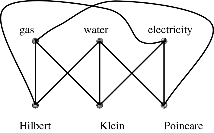
Figure 6: This is no good because we don’t want the lines to intersect.

12 Topology

Topology is the theory of shapes which are allowed to stretch, compress, flex and bend, but without tearing or gluing. For example, a square is topologically equivalent to a circle, since a square can be continously deformed into a circle. As another example, a doughnut and a coffee cup with a handle for are topologically equivalent, since a doughnut can be reshaped into a coffee cup without tearing or gluing.

12.1 Letters

As a starting exercise in topology, let’s look at the letters of the alphabet. We think of the letters as figures made from lines and curves, without fancy doodads such as serifs.

Question. Which of the capital letters are topologically the same, and which are topologically different? How many topologically different capital letters are there?

13 Surfaces

A surface, or 2-manifold, is a shape any small enough neighborhood of which is topologically equivalent to a neighborhood of a point in the plane. For instance, a the surface of a cube is a surface topologically equivalent to the surface of a sphere. On the other hand, if we put an extra wall inside a cube dividing it into two rooms, we no longer have a surface, because there are points at which three sheets come together. No small neighborhood of those points is topologically equivalent to a small neighborhood in the plane.

Figure 7: Here are some pictures of surfaces. The pictures are intended to indicate things like doughnuts and pretzels rather than flat strips of paper. Can you identify these surfaces, topologically? Which ones are topologically the same intrinsically, and which extrinsically?

Recall that you get a torus by identifying the sides of a rectangle as in Figure 2.10 of SS (The Shape of Space). If you identify the sides slightly differently, as in Figure 4.3, you get a surface called a Klein bottle, shown in Figure 4.9.

13.1 Discussion

1. Take some strips and join the opposite ends of each strip together as follows: with no twists; with one twist (half-turn)—this is called a Möbius strip; with two twists; with three twists.

2. Imagine that you are a two-dimensional being who lives in one of these four surfaces. To what extent can you tell exactly which one it is?

3. Now cut each of the above along the midline of the original strip. Describe what you get. Can you explain why?

4. What is the Euler number of a disk? A Möbius strip? A torus with a circular hole cut from it? A Klein bottle? A Klein bottle with a circular hole cut from it?

5. What is the maximum number of points in the plane such that you can draw non-intersecting segments joining each pair of points? What about on a sphere? On a torus?

14 How to knit a Möbius Band

Start with a different color from the one you want to make the band in. Call this the spare color. With the spare color and normal knitting needles cast on 90 stitches.

Change to your main color yarn. Knit your row of 90 stitches onto a circular needle. Your work now lies on about 2/3 of the needle. One end of the work is near the tip of the needle and has the yarn attached. This is the working end. Bend the working end around to the other end of your work, and begin to knit those stitches onto the working end, but do not slip them off the other end of the needle as you normally would. When you have knitted all 90 stitches in this way, the needle loops the work twice.

Carry on knitting in the same direction, slipping stitches off the needle when you knit them, as normal. The needle will remain looped around the work twice. Knit five ‘rows’ (that is $5\times 90$ stitches) in this way.

Cast off. You now have a Mobius band with a row of your spare color running around the middle. Cut out and remove the spare colored yarn. You will be left with one loose stitch in your main color which needs to be secured.

Figure 8: A Mobius band.

(Expanded by Maria Iano-Fletcher from an original recipe by Miles Reid.)

15 Geometry on the sphere

We want to explore some aspects of geometry on the surface of the sphere. This is an interesting subject in itself, and it will come in handy later on when we discuss Descartes’s angle-defect formula.

15.1 Discussion

Great circles on the sphere are the analogs of straight lines in the plane. Such curves are often called geodesics. A spherical triangle is a region of the sphere bounded by three arcs of geodesics.

1. Do any two distinct points on the sphere determine a unique geodesic? Do two distinct geodesics intersect in at most one point?

2. Do any three ‘non-collinear’ points on the sphere determine a unique triangle? Does the sum of the angles of a spherical triangle always equal $\pi$? Well, no. What values can the sum of the angles take on?

The area of a spherical triangle is the amount by which the sum of its angles exceeds the sum of the angles ($\pi$) of a Euclidean triangle. In fact, for any spherical polygon, the sum of its angles minus the sum of the angles of a Euclidean polygon with the same number of sides is equal to its area.

A proof of the area formula can be found in Chapter 9 of Weeks, The Shape of Space.

16 Course projects

We expect everyone to do a project for the course. On the last day of the course, Friday, June 28th, we will hold a Geometry Fair, where projects will be exhibited. Parents and any other interested people are invited.

Here are some ideas, to get you started thinking about possible projects. Be creative—don’t feel limited by these ideas.

• Write a computer program that allows the user to select one of the $17$ planar symmetry groups, start doodling, and see the pattern replicate, as in Escher’s drawings.

• Write a similar program for drawing tilings of the hyperbolic plane, using one or two of the possible hyperbolic symmetry groups.

• Make sets of tiles which exhibit various kinds of symmetry and which tile the plane in various symmetrical patterns.

• Write a computer program that replicates three-dimensional objects according to a three-dimensional pattern, as in the tetrahedron, octahedron, and icosahedron.

• Construct kaleidoscopes for tetrahedral, octahedral and icosahedral symmetry.

• Construct a four-mirror kaleidoscope, giving a three-dimensional pattern of repeating symmetry.

• The Archimidean solids are solids whose faces are regular polygons (but not necessarily all the same) such that every vertex is symmetric with every other vertex. Make models of the the Archimedean solids

• Write a computer program for visualizing four-dimensional space.

• Make stick models of the regular four-dimensional solids.

• Make models of three-dimensional cross-sections of regular four-dimensional solids.

• Design and implement three-dimensional tetris.

• Make models of the regular star polyhedra (Kepler-Poinsot polyhedron).

• Knit a Klein bottle, or a projective plane.

• Make some hyperbolic cloth.

• Sew topological surfaces and maps.

• Infinite Euclidean polyhedra.

• Hyperbolic polyhedra.

• Make a (possibly computational) orrery.

• Design and make a sundial.

• Astrolabe (Like a primitive sextant).

• Calendars: perpetual, lunar, eclipse.

• Cubic surface with 27 lines.

• Spherical Trigonometry or Geometry: Explore spherical trigonometry or geometry. What is the analog on the sphere of a circle in the plane? Does every spherical triangle have a unique inscribed and circumscribed circle? Answer these and other similar questions.

• Hyperbolic Trigonometry or Geometry: Explore hyperbolic trigonometry or geometry. What is the analog in the hyperbolic plane of a circle in the Euclidean plane? Does every hyperbolic triangle have a unique inscribed and circumscribed circle? Answer these and other similar questions.

• Make a convincing model showing how a torus can be filled with circular circles in four different ways.

• Turning the sphere inside out.

• Stereographic lamp.

• Flexible polyhedra.

• Models of ruled surfaces.

• Models of the projective plane.

• Puzzles and models illustrating extrinsic topology.

• Folding ellipsoids, hyperboloids, and other figures.

• Optical models: elliptical mirrors, etc.

• Mechanical devices for angle trisection, etc.

• Panoramic polyhedron (similar to an astronomical globe) made from faces which are photographs.

17 The angle defect of a polyhedron

The angle defect at a vertex of a polygon is defined to be $2\pi$ minus the sum of the angles at the corners of the faces at that vertex. For instance, at any vertex of a cube there are three angles of $\pi/2$, so the angle defect is $\pi/2$. You can visualize the angle defect by cutting along an edge at that vertex, and then flattening out a neighborhood of the vertex into the plane. A little gap will form where the slit is: the angle by which it opens up is the angle defect.

The total angle defect of the polyhedron is gotten by adding up the angle defects at all the vertices of the polyhedron. For a cube, the total angle defect is $8\times\pi/2=4\pi$.

17.1 Discussion

1. What is the angle sum for a polygon (in the plane) with $n$ sides?

2. Determine the total angle defect for each of the 5 regular polyhedra, and for the polyhedra handed out.

18 Descartes’s Formula.

The angle defect at a vertex of a polygon was defined to be the amount by which the sum of the angles at the corners of the faces at that vertex falls short of $2\pi$ and the total angle defect of the polyhedron was defined to be what one got when one added up the angle defects at all the vertices of the polyhedron. We call the total defect $T$. Descartes discovered that there is a connection between the total defect, $T$, and the Euler Number $E-V-F$. Namely,

$$T=2\pi(V-E+F).$$ (1)

Here are two proofs. They both use the fact that the sum of the angles of a polygon with $n$ sides is $(n-2)\pi$.

18.1 First proof

Think of $2\pi(V-E+F)$ as putting $+2\pi$ at each vertex, $-2\pi$ on each edge, and $+2\pi$ on each face.

We will try to cancel out the terms as much as possible, by grouping within polygons.

For each edge, there is $-2\pi$ to allocate. An edge has a polygon on each side: put $-\pi$ on one side, and $-\pi$ on the other.

For each vertex, there is $+2\pi$ to allocate: we will do it according to the angles of polygons at that vertex. If the angle of a polygon at the vertex is $a$, allocate $a$ of the $2\pi$ to that polygon. This leaves something at the vertex: the angle defect.

In each polygon, we now have a total of the sum of its angles minus $n\pi$ (where $n$ is the number of sides) plus $2\pi$. Since the sum of the angles of any polygon is $(n-2)\pi$, this is 0. Therefore,

$$2\pi(V-E+F)=T.$$

18.2 Second proof

We begin to compute:

$$T=\sum_{\hbox{Vertices}}\hbox{the angle defect at the vertex}.$$

$$=\sum_{\hbox{Vertices}}(2\pi-\hbox{the sum of the angles at the corners of those faces that meet at the vertex}).$$

$$=2\pi V-\sum_{\hbox{Vertices}}(\hbox{the sum of the angles at the corners of those faces that meet at the vertex}).$$

$$=2\pi V-\sum_{\hbox{Faces}}\hbox{the sum of the interior angles of the face}.$$

$$=2\pi V-\sum_{\hbox{Faces}}(n_{f}-2)\pi.$$

Here $n_{f}$ denotes the number of edges on the face $f$.

$$T=2\pi V-\sum_{\hbox{Faces}}n_{f}\pi+\sum_{\hbox{Each face}}2\pi.$$

Thus

$$T=2\pi V-(\sum_{\hbox{Faces}}\hbox{the number of edges on the face}\cdot\pi)+2\pi F.$$

If we sum the number of edges on each face over all of the faces, we will have counted each edge twice. Thus

$$T=2\pi V-2E\pi+2\pi F.$$

Whence,

$$T=2\pi(V-E+F).$$

18.3 Discussion

Listen to both proofs given in class.

1. Discuss both proofs with the aim of understanding them.

2. Draw a sketch of the first proof in the blank space above.

3. Discuss the differences between the two proofs. Can you describe the ways in which they are different? Which of you feel the first is easier to understand? Which of you feel the second is easier to understand? Which is more pleasing? Which is more conceptual?

19 Exercises in imagining

How do you imagine geometric figures in your head? Most people talk about their three-dimensional imagination as ‘visualization’, but that isn’t exactly right. A visual image is a kind of picture, and it is really two-dimensional. The image you form in your head is more conceptual than a picture—you locate things in more of a three-dimensional model than in a picture. In fact, it is quite hard to go from a mental image to a two-dimensional visual picture. Children struggle long and hard to learn to draw because of the real conceptual difficulty of translating three-dimensional mental images into two-dimensional images.

Three-dimensional mental images are connected with your visual sense, but they are also connected with your sense of place and motion. In forming an image, it often helps to imagine moving around it, or tracing it out with your hands. The size of an image is important. Imagine a little half-inch sugarcube in your hand, a two-foot cubical box, and a ten-foot cubical room that you’re inside. Logically, the three cubes have the same information, but people often find it easier to manipulate the larger image that they can move around in.

Geometric imagery is not just something that you are either born with or you are not. Like any other skill, it develops with practice.

Below are some images to practice with. Some are two-dimensional, some are three-dimensional. Some are easy, some are hard, but not necessarily in numerical order. Find another person to work with in going through these images. Evoke the images by talking about them, not by drawing them. It will probably help to close your eyes, although sometimes gestures and drawings in the air will help. Skip around to try to find exercises that are the right level for you.

When you have gone through these images and are hungry for more, make some up yourself.

1. Picture your first name, and read off the letters backwards. If you can’t see your whole name at once, do it by groups of three letters. Try the same for your partner’s name, and for a few other words. Make sure to do it by sight, not by sound.

2. Cut off each corner of a square, as far as the midpoints of the edges. What shape is left over? How can you re-assemble the four corners to make another square?

3. Mark the sides of an equilateral triangle into thirds. Cut off each corner of the triangle, as far as the marks. What do you get?

4. Take two squares. Place the second square centered over the first square but at a forty-five degree angle. What is the intersection of the two squares?

5. Mark the sides of a square into thirds, and cut off each of its corners back to the marks. What does it look like?

6. How many edges does a cube have?

7. Take a wire frame which forms the edges of a cube. Trace out a closed path which goes exactly once through each corner.

8. Take a $3\times 4$ rectangular array of dots in the plane, and connect the dots vertically and horizontally. How many squares are enclosed?

9. Find a closed path along the edges of the diagram above which visits each vertex exactly once? Can you do it for a $3\times 3$ array of dots?

10. How many different colors are required to color the faces of a cube so that no two adjacent faces have the same color?

11. A tetrahedron is a pyramid with a triangular base. How many faces does it have? How many edges? How many vertices?

12. Rest a tetrahedron on its base, and cut it halfway up. What shape is the smaller piece? What shapes are the faces of the larger pieces?

13. Rest a tetrahedron so that it is balanced on one edge, and slice it horizontally halfway between its lowest edge and its highest edge. What shape is the slice?

14. Cut off the corners of an equilateral triangle as far as the midpoints of its edges. What is left over?

15. Cut off the corners of a tetrahedron as far as the midpoints of the edges. What shape is left over?

16. You see the silhouette of a cube, viewed from the corner. What does it look like?

17. How many colors are required to color the faces of an octahedron so that faces which share an edge have different colors?

18. Imagine a wire is shaped to go up one inch, right one inch, back one inch, up one inch, right one inch, back one inch, …. What does it look like, viewed from different perspectives?

19. The game of tetris has pieces whose shapes are all the possible ways that four squares can be glued together along edges. Left-handed and right-handed forms are distinguished. What are the shapes, and how many are there?

20. Someone is designing a three-dimensional tetris, and wants to use all possible shapes formed by gluing four cubes together. What are the shapes, and how many are there?

21. An octahedron is the shape formed by gluing together equilateral triangles four to a vertex. Balance it on a corner, and slice it halfway up. What shape is the slice?

22. Rest an octahedron on a face, so that another face is on top. Slice it halfway up. What shape is the slice?

23. Take a $3\times 3\times 3$ array of dots in space, and connect them by edges up-and-down, left-and-right, and forward-and-back. Can you find a closed path which visits every dot but one exactly once? Every dot?

24. Do the same for a $4\times 4\times 4$ array of dots, finding a closed path that visits every dot exactly once.

25. What three-dimensional solid has circular profile viewed from above, a square profile viewed from the front, and a triangular profile viewed from the side? Do these three profiles determine the three-dimensional shape?

26. Find a path through edges of the dodecahedron which visits each vertex exactly once.

20 Curvature of surfaces

If you take a flat piece of paper and bend it gently, it bends in only one direction at a time. At any point on the paper, you can find at least one direction through which there is a straight line on the surface. You can bend it into a cylinder, or into a cone, but you can never bend it without crumpling or distorting to the get a portion of the surface of a sphere.

If you take the skin of a sphere, it cannot be flattened out into the plane without distortion or crumpling. This phenomenon is familiar from orange peels or apple peels. Not even a small area of the skin of a sphere can be flattened out without some distortion, although the distortion is very small for a small piece of the sphere. That’s why rectangular maps of small areas of the earth work pretty well, but maps of larger areas are forced to have considerable distortion.

The physical descriptions of what happens as you bend various surfaces without distortion do not have to do with the topological properties of the surfaces. Rather, they have to do with the intrinsic geometry of the surfaces. The intrinsic geometry has to do with geometric properties which can be detected by measurements along the surface, without considering the space around it.

There is a mathematical way to explain the intrinsic geometric property of a surface that tells when one surface can or cannot be bent into another. The mathematical concept is called the Gaussian curvature of a surface, or often simply the curvature of a surface. This kind of curvature is not to be confused with the curvature of a curve. The curvature of a curve is an extrinsic geometric property, telling how it is bent in the plane, or bent in space. Gaussian curvature is an intrinsic geometric property: it stays the same no matter how a surface is bent, as long as it is not distorted, neither stretched or compressed.

To get a first qualitative idea of how curvature works, here are some examples.

A surface which bulges out in all directions, such as the surface of a sphere, is positively curved. A rough test for positive curvature is that if you take any point on the surface, there is some plane touching the surface at that point so that the surface lies all on one side except at that point. No matter how you (gently) bend the surface, that property remains.

A flat piece of paper, or the surface of a cylinder or cone, has 0 curvature.

A saddle-shaped surface has negative curvature: every plane through a point on the saddle actually cuts the saddle surface in two or more pieces.

Question. What surfaces can you think of that have positive, zero, or negative curvature.

Gaussian curvature is a numerical quantity associated to an area of a surface, very closely related to angle defect. Recall that the angle defect of a polyhedron at a vertex is the angle by which a small neighborhood of a vertex opens up, when it is slit along one of the edges going into the vertex.

The total Gaussian curvature of a region on a surface is the angle by which its boundary opens up, when laid out in the plane. To actually measure Gaussian curvature of a region bounded by a curve, you can cut out a narrow strip on the surface in neighborhood of the bounding curve. You also need to cut open the curve, so it will be free to flatten out. Apply it to a flat surface, being careful to distort it as little as possible. If the surface is positively curved in the region inside the curve, when you flatten it out, the curve will open up. The angle between the tangents to the curve at the two sides of the cut is the total Gaussian curvature. This is like angle defect: in fact, the total curvature of a region of a polyhedron containing exactly one vertex is the angle defect at that vertex. You must pay attention pay attention not just to the angle between the ends of the strip, but how the strip curled around, keeping in mind that the standard for zero curvature is a strip which comes back and meets itself. Pay attention to $\pi$’s and $2\pi$’s.

Figure 9: This diagram illustrates how to measure the total Gaussian curvature of a patch by cutting out a strip which bounds the patch, and laying it out on a flat surface. The angle by which the strip ‘opens up’ is the total Gaussian curvature. You must pay attention not just to the angle between the lines on the paper, but how it got there, keeping in mind that the standard for zero curvature is a strip which comes back and meets itself. Pay attention to $\pi$’s and $2\pi$’s.

If the total curvature inside the region is negative, the strip will curl around further than necessary to close. The curvature is negative, and is measured by the angle by which the curve overshoots.

A less destructive way to measure total Gaussian curvature of a region is to apply narrow strips of paper to the surface, e.g., masking tape. They can be then be removed and flattened out in the plane to measure the curvature.

Question. Measure the total Gaussian curvature of

1. a cabbage leaf.

2. a kale leaf

3. a piece of banana peel

4. a piece of potato skin

If you take two adjacent regions, is the total curvature in the whole equal to the sum of the total curvature in the parts? Why?

The angle defect of a convex polyhedron at one of its vertices can be measured by rolling the polyhedron in a circle around its vertex. Mark one of the edges, and rest it on a sheet of paper. Mark the line on which it contacts the paper. Now roll the polyhedron, keeping the vertex in contact with the paper. When the given edge first touches the paper again, draw another line. The angle between the two lines (in the area where the polyhedron did not touch) is the angle defect. In fact, the area where the polyhedron did touch the paper can be rolled up to form a paper model of a neighborhood of the vertex in question.

A polyhedron can also be rolled in a more general way. Mark some closed path on the surface of the polyhedron, avoiding vertices. Lay the polyhedron on a sheet of paper so that part of the curve is in contact. Mark the position of one of the edges in contact with the paper. now roll the polyhedron, along the curve, until the original face is in contact again, and mark the new position of the same edge. What is the angle between the original position of the line, and the new position of the line?

21 Gaussian curvature

21.1 Discussion

1. What is the curvature inside the region on a sphere exterior to a tiny circle?

2. On a polyhedron, what is the curvature inside a region containing a single vertex? two vertices? all but one vertex? all the vertices?

22 Clocks and curvature

The total curvature of any surface topologically equivalent to the sphere is $4\pi$. This can be seen very simply from the definition of the curvature of a region in terms of the angle of rotation when the surface is rolled around on the plane; the only problem is the perennial one of keeping proper track of multiples of $\pi$ when measuring the angle of rotation. Since are trying to show that the total curvature is a specific multiple of $\pi$, this problem is crucial. So to begin with let’s think carefully about how to reckon these angles correctly

22.1 Clocks

Suppose we have a number of clocks on the wall. These clocks are good mathematician’s clocks, with a 0 up at the top where the 12 usually is. (If you think about it, 0 o’clock makes a lot more sense than 12 o’clock: With the 12 o’clock system, a half hour into the new millennium on 1 Jan 2001, the time will be 12:30 AM, the 12 being some kind of hold-over from the departed millennium.)

Let the clocks be labelled $A$, $B$, $C$, …. To start off, we set all the clocks to 0 o’clock. (little hand on the 0; big hand on the 0), Now we set clock $B$ ahead half an hour so that it now the time it tells is 0:30 (little hand on the 0 (as they say); big hand on the 6). What angle does its big hand make with that of clock $A$? Or rather, through what angle has its big hand moved relative to that of clock $A$? The angle is $\pi$. If instead of degrees or radians, we measure our angles in revs (short for revolutions), then the angle is $1/2$ rev. We could also say that the angle is $1/2$ hour: as far as the big hand of a clock is concerned, an hour is the same as a rev.

Now take clock $C$ and set it to 1:00. Relative to the big hand of clock $A$, the big hand of $C$ has moved through an angle of $2\pi$, or 1 rev, or 1 hour. Relative to the big hand of $B$, the big hand of $C$ has moved through an angle of $\pi$, or $1/2$ rev. Relative to the big hand of $C$, the big hand of $A$ has moved through an angle of $-2\pi$, or $-1$ rev, and the big hand of $B$ has moved $-\pi$, or $-1$ rev.

22.2 Curvature

Now let’s describe how to find the curvature inside a disk-like region $R$ on a surface $S$, i.e. a region topologically equivalent to a disk. What we do is cut a small circular band running around the boundary of the region, cut the band open to form a thin strip, lay the thin strip flat on the plane, and measure the angle between the lines at the two end of the strip. In order to keep the $\pi$’s straight, let us go through this process very slowly and carefully.

To begin with, let’s designate the two ends of the strip as the left end and the right end in such a way that traversing the strip from the left end to the right end corresponds to circling clockwise around the region. We begin by fixing the left-hand end of the strip to the wall so that the straight edge of the cut at the left end of the strip—the cut that we made to convert the band into a strip—runs straight up and down, parallel to the big hand of clock $A$, and so that the strip runs off toward the right. Now we move from left to right along the strip, i.e. clockwise around the boundary of the region, fixing the strip so that it lies as flat as possible, until we come to the right end of the strip. Then we look at the cut bounding the right-hand end of the strip, and see how far it has turned relative to the left-hand end of the strip. Since we were so careful in laying out the left-hand end of the strip, our task in reckoning the angle of the right-hand end of the strip amounts to deciding what time you get if you think of the right-hand end of the strip as the big hand of a clock. The curvature inside the region will correspond to the amount by which the time told by the right-hand end of the strip falls short of 1:00.

For instance, say the region $R$ is a tiny disk in the Euclidean plane. When we cut a strip from its boundary and lay it out as described above, the time told by its right hand end will be precisely 1:00, so the curvature of $R$ will be exactly 0. If $R$ is a tiny disk on the sphere, then when the strip is laid out the time told will be just shy of 1:00, say 0:59, and the curvature of the region will be $\frac{1}{60}$ rev, or $\frac{\pi}{30}$.

When the region $R$ is the lower hemisphere of a round sphere, the strip you get will be laid out in a straight line, and the time told by the right-hand end will be 0:00, so the total curvature will be 1 rev, i.e. $2\pi$. The total curvature of the upper hemisphere is $2\pi$ as well, so that the total curvature of the sphere is $4\pi$.

Another way to see that the total curvature of the sphere is $4\pi$ is to take as the region $R$ the outside of a small circle on the sphere. When we lay out a strip following the prescription above, being sure to traverse the boundary of the region $R$ in the clockwise sense as viewed from the point of view of the region $R$, we see that the time told by the right hand end of the strip is very nearly $-1$ o’clock! The precise time will be just shy of this, say $-1$:59, and the total curvature of the region will then be $1\frac{59}{60}$ revs. Taking the limit, the total curvature of the sphere is 2 revs, or $4\pi$.

But this last argument will work equally well on any surface topologically equivalent to a sphere, so any such surface has total curvature $4\pi$.

22.3 Where’s the beef?

This proof that the total curvature of a topological sphere is $4\pi$ gives the definite feeling of being some sort of trick. How can we get away without doing any work at all? And why doesn’t the argument work equally well on a torus, which as we know should have total curvature 0? What gives?

What gives is the lemma that states that if you take a disklike region $R$ and divide it into two disklike subregions $R_{1}$ and $R_{2}$, then the curvature inside $R$ when measured by laying out its boundary is the sum of the curvatures inside $R_{1}$ and $R_{2}$ measured in this way. This lemma might seem like a tautology. Why should there be anything to prove here? How could it fail to be the case that the curvature inside the whole is the sum of the curvatures inside the parts? The answer is, it could fail to be the case by virtue of our having given a faulty definition. When we define the curvature inside a region, we have to make sure that the quantity we’re defining has the additivity property, or the definition is no good. Simply calling some quantity the curvature inside the region will not make it have this additivity property. For instance, what if we had defined the curvature inside a region to be $4\pi$, no matter what the region? More to the point, what if in the definition of the curvature inside a region we had forgotten the proviso that the region $R$ be disklike? Think about it.

23 Photographic polyhedron

As you stand in one place and look around, up, and down, there is a sphere’s worth of directions you can look. One way to record what you see would be to construct a big sphere, with the image painted on the inside surface. To see the world as viewed from the one place, you would stand on a platform in the center of the sphere and look around. We will call this sphere the visual sphere. You can imagine a sphere, like a planetarium, with projectors projecting a seamless image. The image might be created by a robotic camera device, with video cameras pointing in enough directions to cover everything.

Question. What is the geometric relation of objects in space to their images on the visual sphere?

1. Show that the image of a line is an arc of a great circle. If the line is infinitely long, how long (in degrees) is the arc of the circle?

2. Describe the image of several parallel lines.

3. What is the image of a plane?

Unfortunately, you can’t order spherical prints from most photographic shops. Instead, you have to settle for flat prints. Geometrically, you can understand the relation of a flat print to the ‘ideal’ print on a spherical surface by constructing a plane tangent to the sphere at a point corresponding to the center of the photograph. You can project the surface of the sphere outward to the plane, by following straight lines from the center of the sphere to the surface of the sphere, and then outward to the plane. From this, you can see that given size objects on the visual sphere do not always come out the same size on a flat print. The further they are from the center of the photograph, the larger they are on the print.

Suppose we stand in one place, and take several photographs that overlap, so as to construct a panorama. If the camera is adjusted in exactly the same way for the various photographs, and the prints are made in exactly the same way, the photographs can be thought of as coming from rectangles tangent to a copy of the visual sphere, of some size. The exact radius of this sphere, the photograph sphere depends on the focal length of the camera lens, the size of prints, etc., but it should be the same sphere for all the different prints.

If we try to just overlap them on a table and glue them together, the images will not match up quite right: objects on the edge of a print are larger than objects in the middle of a print, so they can never be exactly aligned.

Instead, we should try to find the line where two prints would intersect if they were arranged to be tangent to the sphere. This line is equidistant from the centers of the two prints. You can find it by approximately aligning the two prints on a flat surface, draw the line between the centers of the prints, and constructing the perpendicular bisector. Cut along this line on one of the prints. Now find the corresponding line on the other print. These two lines should match pretty closely. This process can be repeated: now that the two prints have a better match, the line segment between their centers can be constructed more accurately, and the perpendicular bisector works better.

If you perform this operation for a whole collection of photographs, you can tape them together to form a polyhedron. The polyhedron should be circumscribed about a certain size sphere. It can give an excellent impression of a wide-angle view of the scene. If the photographs cover the full sphere, you can assemble them so that the prints are face-outwards. This makes a globe, analogous to a star globe. As you turn it around, you see the scene in different directions. If the photographs cover a fair bit less than a full sphere, you can assemble them face inwards. This gives a better wide-angle view.

One way to do this is just to take enough photographs that you cover a certain area of the visual sphere, match them up, cut them out, and tape them together. The polyhedron you get in this way will probably not be very regular.

By choosing carefully the directions in which you take photographs, you could make the photographic polyhedron have a regular, symmetric structure. Using an ordinary lens, a photograph is not wide enough to fill the face of any of the 5 regular polyhedra.

An Archimedean polyhedron is a polyhedron such that every face is a regular polygon (but not necessarily all the same), and every vertex is symmetric with every other vertex. For instance, the soccer ball polyhedron, or truncated icosahedron, is Archimedean.

Question. Show that every Archimedean polyhedron is inscribed in a sphere.

The dual Archimedean polyhedra are polyhedra which are dual to Archimedean polyhedra.

Question.

• Show that each of the dual Archimedean polyhedra can be circumscribed about a sphere.

• Which polyhedra will work well to make a photographic polyhedron?

24 Mirrors

24.1 Discussion

1. How do you hold two mirrors so as to get an integral number of images of yourself? Discuss the handedness of the images.

2. Set up two mirrors so as to make perfect kaleidoscopic patterns. How can you use them to make a snowflake?

3. Fold and cut hearts out of paper. Then make paper dolls. Then honest snowflakes.

4. Set up three or more mirrors so as to make perfect kaleidoscopic patterns. Fold and cut such patterns out of paper.

5. Why does a mirror reverse right and left rather than up and down?

25 More paper-cutting patterns

Experiment with the constructions below. Put the best examples into your journal, along with comments that describe and explain what is going on. Be careful to make your examples large enough to illustrate clearly the symmetries that are present. Also make sure that your cuts are interesting enough so that extra symmetries do not creep in. Concentrate on creating a collection of examples that will get across clearly what is going on, and include enough written commentary to make a connected narrative.

1. Conical patterns. Many rotationally-symmetric designs, like the twin blades of a food processor, cannot be made by folding and cutting. However, they can be formed by wrapping paper into a conical shape.

   Fold a sheet of paper in half, and then unfold. Cut along the fold to the center of the paper. Now wrap the paper into a conical shape, so that the cut edge lines up with the uncut half of the fold. Continue wrapping, so that the two cut edges line up and the original sheet of paper wraps two full turns around a cone. Now cut out any pattern you like from the cone. Unwrap and lay it out flat. The resulting pattern should have two-fold rotational symmetry.

   Try other examples of this technique, and also try experimenting with rolling the paper more than twice around a cone.

2. Cylindrical patterns. Similarly, it is possible to make repeating designs on strips. If you roll a strip of paper into a cylindrical shape, cut it, and unroll it, you should get a repeating pattern on the edge. Try it.

3. Möbius patterns. A Möbius band is formed by taking a strip of paper, and joining one end to the other with a twist so that the left edge of the strip continues to the right.

   Make or round up a strip of paper which is long compared to its width (perhaps made from ribbon, computer paper, adding-machine rolls, or formed by joining several shorter strips together end-to-end). Coil it around several times around in a Möbius band pattern. Cut out a pattern along the edge of the Möbius band, and unroll.

4. Other patterns. Can you come up with any other creative ideas for forming symmetrical patterns?

26 Summary

In the past week we have discussed a number of different topics, many of which seemed to be unrelated. When we began last week, we said that we would jump around from topic to topic during the first few days so that you would become familiar with a number of different ideas and examples. What we want to do today is to show you that there really is a method to our madness and that there is a connection between these seemingly diverse bits of mathematics and that the connection is one of the most deep and beautiful ones in mathematics. Virtually any property (visual or otherwise) that one naively chooses as a way to describe (and quantify) a surface is related in a simple way to any other property one naively chooses and duly quantifies. Here is a list of some of the things we touched upon last week.

• The Euler Number

• Flashlights

• Proofs of the angular defect formula

• Maps on surfaces

• Area of a spherical triangle

• Cabbage

• Curvature

• The Gauss map

• Handle, holes, surfaces

• Kale

• Orientability

27 The Euler Number

If we have a polyhedron, we can compute its Euler number, $\chi=V-E+F$. In fact, we computed Euler numbers ad delectam. Why did we do this? One reason is that they are easy to compute. But that is not obviously a compelling reason for doing anything in mathematics. The real reason is that it is an invariant of the surface (it does not depend upon what map one puts on the surface) and because it is connected to a whole array of other properties a surface might have that one might notice while trying to describe it.

27.1 Descartes’s Formula

One easy example of this is Descartes’ formula. If one looks at a polyhedral surface and makes a naive attempt to describe it visually, one might try to describe how pointy the surface is. A more sophisticated way to describe how pointy a surface is at a vertex is to compute the angular defect at the vertex, that is

$$2\pi-(\hbox{ the sum of the angles of the faces meeting at the vertex }).$$

When we investigated how pointy a polyhedron was, summing over all of the vertices to obtain the total angular defect $T$, we discovered that there was a direct connection between pointyness and Euler Number:

$$T=2\pi(V-E+F).$$

27.2 The Gauss Map (Flashlights)

Although projecting Conway’s image onto the celestial sphere was fun, again it was not in and of itself a mathematically valuable exercise. The point was to get a feel for the Gauss map. The Gauss map is used to project a surface onto the celestial sphere. For a polyhedron, we saw that, if one traced a path that remained on a flat face, the Gauss image of that path was really a point. We saw that if we traced a path that went around a vertex, the Gauss image was a spherical polygon. If three edges met at the given vertex, the Gauss image traced out a spherical triangle whose interior could be thought of as the image of that vertex. Moreover, the angles of the triangle were the supplements of the vertex angles. Using the formula for the area of a spherical triangle, namely

$$(\hbox{ the sum of the angles })-\pi,$$

if the vertex angles were $\alpha,\beta,\hbox{ and }\gamma$, the area of the Gauss image of a path around the vertex would be

$$\{(\pi-\alpha)+(\pi-\beta)+(\pi-\gamma)\}-\pi=2\pi-(\alpha+\beta+\gamma).$$

The right hand side of this formula is just the angular defect at the vertex. Thus if we add up the areas of the images of path about all of the vertices, we obtain the total defect $T$ of the original surface. Since no other parts of the image contribute to the area, we have shown that

$$\hbox{\bf the area of the Gauss image }=T.$$

Exploiting the earlier connection, we can also say

$$\hbox{\bf the area of the Gauss image }=2\pi(V-E+F).$$

This is known as the Gauss-Bonnet formula.

27.3 Curvature (Kale and cabbage)

Again, cutting up kale and cabbage was fun and the tape of Thurston and Conway sticking potato peel to the chalkboard will become a classic, but there was a serious mathematical purpose behind it. If one looks at a surface and wants to try to describe it visually, one might want to describe it by telling how curly it is. While the surface of a cylinder, for example, does not look visually as though it curves and bends very much, the surface of a trumpet does. Peeling a surface, that is, removing a thin strip from around a portion of the surface and then seeing how much the angle between the ends of the strip opens up (or closes around) as it is laid flat quantifies the curviness of the portion of the surface surrounded by the strip. Mathematically, this is called the integrated curvature of that portion of the surface.

When we sum over portions that amount to the whole surface, we get the total Gaussian curvature of the surface.

27.3.1 Curvature for Polyhedra

Lets apply these ideas to a polyhedron. In particular, we might consider a strip of polyhedron peel that just goes around one vertex of a polyhedron. Then we would find that the path opens up by an angle equal to the defect at that vertex, and so for such a path

the total curvature enclosed

$$=\hbox{ the defect at the enclosed vertex }$$

$$=\hbox{ the area of the Gauss image }.$$

For a path that goes around several vertices the curvature is the sum of the defects of all the surrounded vertices. Thus for a polyhedron,

$$K=\hbox{\bf Total Gaussian Curvature}=T.$$

27.3.2 Curvature on surfaces

To pass from a polyhedral surface to a smooth surface and to define curvature with mathematical precision, one needs to use integration in the definition for $K$. But the conceptual idea is still the same. Any curved surface can be approximated by a polyhedral one with lots and lots of vertices. The curvature of the surface within a path (a smooth piece of peel) is then very nearly equal to the sum of the defects at all the encircled vertices. By a technical limiting argument that involves integrals to give a precise meaning to curvature, $K$, we find that for any surface

$$K=\hbox{\bf Total Gaussian Curvature}=T.$$

27.4 Discussion

• There are many other connections between these four concepts. Can you suggest any more? (This is also a discussion question for the gang of four.)

• The number of handles on a surface is another visual characteristic. How does this relate to the total curvature?

28 Symmetry and orbifolds

Given a symmetric pattern, what happens when you identify equivalent points? It gives an object with interesting topological and geometrical properties, called an orbifold.

The first instance of this is an object with bilateral symmetry, such as a (stylized) heart. Children learn to cut out a heart by folding a sheet of paper in half, and cutting out half of the pattern. When you identify equivalent points, you get half a heart.

Figure 10: A heart is obtained by folding a sheet of paper in half, and cutting out half a heart. The half-heart is the orbifold for the pattern. A heart can also be recreated from a half-heart by holding it up to a mirror.

A second instance is the paper doll pattern. Here, there are two different fold lines. You make paper dolls by folding a strip of paper zig-zag, and then cutting out half a person. The half-person is enough to reconstruct the whole pattern. The quotient orbifold is a half-person, with two mirror lines.

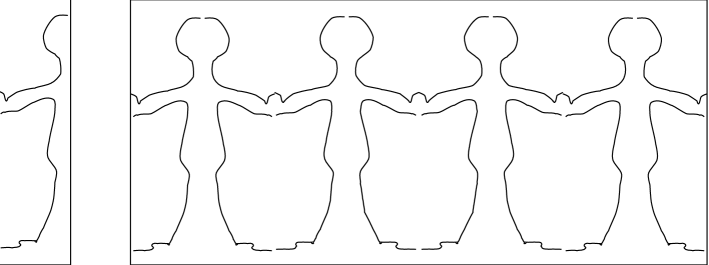
Figure 11: A string of paper dolls

A wave pattern is the next example. This pattern repeats horizontally, with no reflections or rotations. The wave pattern can be rolled up into a cylinder. It can be constructed by rolling up a strip of paper around a cylinder, and cutting a single wave, through several layers, with a sharp knife. When it is unrolled, the bottom part will be like the waves.

Figure 12: This wave pattern repeats horizontally, with no reflections or rotations. The quotient orbifold is a cylinder.

When a pattern repeats both horizontally and vertically, but without reflections or rotations, the quotient orbifold is a torus. You can think of it by first rolling up the pattern in one direction, matching up equivalent points, to get a long cylinder. The cylinder has a pattern which still repeats vertically. Now coil the cylinder in the other direction to match up equivalent points on the cylinder. This gives a torus.

Figure 13: This pattern has quotient orbifold a torus. It repeats both horizontally and vertically, but without any reflections or rotations. It can be rolled up horizontally to form a cylinder, and then vertically (with a twist) to form a torus.

Figure 14: The quotient orbifold is a rectangle, with four mirrors around it.

Figure 15: The quotient orbifold is an annulus, with two mirrors, one on each boundary.

Figure 16: The quotient orbifold is a Moebius band, with a single mirror on its single boundary.

Figure 17: The quotient orbifold is a $60^{\circ}$, $30^{\circ}$, $90^{\circ}$ triangle, with three mirrors from sides.

Figure 18: This pattern has rotational symmetry about various points, but no reflections. The rotations are of order 6, 3 and 2. The quotient orbifold is a triangular pillow, with three cone points.

28.1 Discussion

Using the notation we have discussed, try to figure out the description of the various pieces of fabric we have handed out. That is, locate the mirror strings, gyration points, cone points, etc. Find the orders of the gyration points and the cone points.

29 Names for features of symmetrical patterns

We begin by introducing names for certain features that may occur in symmetrical patterns. To each such feature of the pattern, there is a corresponding feature of the quotient orbifold, which we will discuss later.

29.1 Mirrors and mirror strings

A mirror is a line about which the pattern has mirror symmetry. Mirrors are perhaps the easiest features to pick out by eye.

At a crossing point, where two or more mirrors cross, the pattern will necessarily also have rotational symmetry. An $n$-way crossing point is one where precisely $n$ mirrors meet. At an $n$-way crossing point, adjacent mirrors meet at an angle of $\pi/n$. (Beware: at a 2-way crossing point, where two mirrors meet at right angles, there will be 4 slices of pie coming together.)

We obtain a mirror string by starting somewhere on a mirror and walking along the mirror to the next crossing point, turning as far right as we can so as to walk along another mirror, walking to the next crossing point on it, and so on. (See figure 19.)

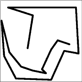
Figure 19: The quotient billiard orbifold.

Suppose that you walk along a mirror string until you first reach a point exactly like the one you started from. If the crossings you turned at were (say) a 6-way, then a 3-way, and then a 2-way crossing, then the mirror string would be of type $*632$, etc. As a special case, the notation $*$ denotes a mirror that meets no others.

For example, look at a standard brick wall. There are horizontal mirrors that each bisect a whole row of bricks, and vertical mirrors that pass through bricks and cement alternately. The crossing points, all 2-way, are of two kinds: one at the center of a brick, one between bricks. The mirror strings have four corners, and you might expect that their type would be $*2222$. However, the correct type is $*22$. The reason is that after going only half way round, we come to a point exactly like our starting point.

29.2 Mirror boundaries

In the quotient orbifold, a mirror string of type $*abc$ becomes a boundary wall, along which there are corners of angles $\pi/a,\pi/b,\pi/c$. We call this a mirror boundary of type $*abc$. For example, a mirror boundary with no corners at all has type $*$. The quotient orbifold of a brick wall has a mirror boundary with just two right-angled corners, type $*22$.

29.3 Gyration points

Any point around which a pattern has rotational symmetry is called a rotation point. Crossing points are rotation points, but there may also be others. A rotation point that does NOT lie on a mirror is called a gyration point. A gyration point has order $n$ if the smallest angle of any rotation about it is $2\pi/n$.

For example, on our brick wall there is an order 2 gyration point in the middle of the rectangle outlined by any mirror string.

29.4 Cone points

In the quotient orbifold, a gyration point of order $n$ becomes a cone point with cone angle $2\pi/n$.

30 Names for symmetry groups and orbifolds

A symmetry group is the collection of all symmetry operations of a pattern. We give the same names to symmetry groups as to the corresponding quotient orbifolds.

We regard every orbifold as obtained from a sphere by adding cone-points, mirror boundaries, handles, and cross-caps. The major part of the notation enumerates the orders of the distinct cone points, and then the types of all the different mirror boundaries. An initial black spot $\bullet$ indicates the addition of a handle; a final circle $\circ$ the addition of a cross cap.

For example, our brick wall gives $2*22$, corresponding to its gyration point of order 2, and its mirror string with two 2-way corners.

Here are the types of some of the patterns shown in section 31:

Figure 14: $\bullet$; Figure 15: $*2222$; Figure 16: $**$; Figure 17: $*\circ$. Figure 18: $*632$. Figure 19: $632$.

Appart from the spots and circles, these can be read directly from the pictures: The important thing to remember is that if two things are equivalent by a symmetry, then you only record one of them. A dodecahedron is very like a sphere. The orbifold corresponding to its symmetry group is a spherical triangle having angles $\pi/5,\pi/3,\pi/2$; so its symmetry group is $*532$.

You, the topologically spherical reader, approximately have symmetry group $*$, because the quotient orbifold of a sphere by a single reflection is a hemisphere whose mirror boundary has no corners.

31 Stereographic Projection

We let $G$ be a sphere in Euclidean three space. We want to obtain a picture of the sphere on a flat piece of paper or a plane. Whenever one projects a higher dimensional object onto a lower dimensional object, some type of distortion must occur. There are a number of different ways to project and each projection preserves some things and distorts others. Later we will explain why we choose stereographic projection, but first we describe it.

31.1 Description

We shall map the sphere $G$ onto the plane containing its equator. Connect a typical point $P$ on the surface of the sphere to the north pole $N$ by a straight line in three space. This line will intersect the equatorial plane at some point $P^{\prime}$. We call $P^{\prime}$ the projection of $P$.

Using this recipe every point of the sphere except the North pole projects to some point on the equatorial plane. Since we want to include the North pole in our picture, we add an extra point $\infty$, called the point at infinity, to the equatorial plane and we view $\infty$ as the image of $N$ under stereographic projection.

31.2 Discussion

• Take $G$ to be the unit sphere, $\{(x,y,z)|x^{2}+y^{2}+z^{2}=1\}$ so that $xy$ plane is the equatorial plane. The typical point $P$ on the sphere has coordinates $(X,Y,Z)$. The typical point $P^{\prime}$ in the equatorial plane, whose coordinates are $(x,y,0)$, will be called $(x,y)$.

  1. Show that the South pole is mapped into the origin under stereographic projection.

  2. Show that under stereographic projection the equator is mapped onto the unit circle, that is the circle $x^{2}+y^{2}=1$.

  3. Show that under stereographic projection the lower hemisphere is mapped into the interior of this circle, that is the disk $D=\{(x,y)|x^{2}+y^{2}<1\}$.

  4. Show that under stereographic projection the upper hemisphere is mapped into the exterior of this circle, that is into $\{(x,y)|x^{2}+y^{2}>1\}$.

     For this to be true where do we have to think of $\infty$ as lying: interior to $D$ or exterior to it?

  5. What projects on to the $x$-axis?

     What projects onto the $x-\hbox{axis }\cup\infty$? Call the set of points that project onto $x-\hbox{axis }\cup\infty$ the prime meridian.

  6. The prime meridian divides the sphere into two hemispheres, the front hemisphere and the back hemisphere. What is the image of the back hemisphere under stereographic projection? The front hemisphere?

  7. Under stereographic projection what is the image of a great circle passing through the north pole? Of any circle (not necessarily a great circle) passing through the north pole?

  8. Under stereographic projection, what projects onto the $y$-axis? onto any vertical line, not necessarily the $y$ axis?

31.3 What’s good about stereographic projection?

Stereographic projection preserves circles and angles. That is, the image of a circle on the sphere is a circle in the plane and the angle between two lines on the sphere is the same as the angle between their images in the plane. A projection that preserves angles is called a conformal projection.

We will outline two proofs of the fact that stereographic projection preserves circles, one algebraic and one geometric. They appear below.

Before you do either proof, you may want to clarify in your own mind what a circle on the surface of a sphere is. A circle lying on the sphere is the intersection of a plane in three space with the sphere. This can be described algebraically. For example, the sphere of radius 1 with center at the origin is given by

$$G=\{(X,Y,Z)|X^{2}+Y^{2}+Z^{2}=1\}.$$ (2)

An arbitrary plane in three-space is given by

$$AX+BY+CZ+D=0$$ (3)

for some arbitrary choice of the constants $A$,$B$, $C$, and $D$. Thus a circle on the unit sphere is any set of points whose coordinates simultaneously satisfy equations  2 and  3.

31.3.1 The algebraic proof

The fact that the points $P$, $P^{\prime}$ and $N$ all lie on one line can be expressed by the fact that

$$(X,Y,Z-1)=t(x,y,-1)$$ (4)

for some non-zero real number $t$. (Here $P=(X,Y,Z),N=(0,0,1),\hbox{ and }P^{\prime}=(x,y,0)$.)

The idea of the proof is that one can use equations  2 and  4 to write $X$ as a function of $t$ and $x$, $Y$ as a function of $t$ and $y$, and $Z$ as a function of $t$ and to simplify equation  3 to an equation in $x$ and $y$. Since the equation in $x$ and $y$ so obtained is clearly the equation of a circle in the $xy$ plane, the projection of the intersection of  2 and  3 is a circle.

To be more precise:

Equation  4 says that $X=tx,Y=ty,\hbox{ and }1-Z=t$. Set $Q=\frac{1+Z}{1-Z}$ and verify that

$$Z=\frac{Q-1}{Q+1},1+Q=\frac{2}{t},\hbox{ and }Q=x^{2}+y^{2}.$$

If $P$ lies on the plane,

$$AX+BY+CZ+D=0.$$

Thus

$$Atx+Bty+C\frac{Q-1}{Q+1}+D=0.$$

Or

$$\frac{2Ax}{Q+1}+\frac{2By}{Q+1}+C\frac{Q-1}{Q+1}+D=0.$$

Whence,

$$2Ax+2By+C(Q-1)+D(Q+1)=0.$$

Or

$$(C+D)Q+2Ax+2By+D-C=0.$$

Recalling that $Q=x^{2}+y^{2}$, we see

$$(C+D)(x^{2}+y^{2})+2Ax+2By+D-C=0$$ (5)

Since the coefficients of the $x^{2}$ and the $y^{2}$ terms are the same, this is the equation of a circle in the plane.

31.3.2 The geometric proofs

The geometric proofs sketched below use the following principle:

It doesn’t really make much difference if instead of projecting onto the equatorial plane, we project onto another horizontal plane (not through N), for example the plane that touches the sphere at the South pole, S. Just what difference does this make?

• Angles: To see that stereographic projection preserves angles at $P$, we project onto the horizontal plane $H$ through $P$. Then by symmetry the tangent planes $tN$ and $tP$ at $N$ and $P$ make the same angle $\phi$ with $NP$, as also does $H$, by properties of parallelism (see figure # 1 at the end of this handout).

  So $tP$ and $H$ are images of each other in the (“mirror”) plane $M$ through $P$ and perpendicular to $NP$.

  For a point $Q$ on the sphere near $P$, the line $NQ$ is nearly parallel to $NP$, so that for points near $P$, stereographic projection is approximately the reflection in $M$.

• Circles: To see that stereographic projection takes circles to circles, first note that any circle $C$ is where some cone touches the sphere, say the cone of tangent lines to the sphere from a point $V$.

  Now project onto the horizontal plane $H$ through $V$.

  In figure # 2 which NEED NOT be a vertical plane, the four angles $\phi$ are equal, for the same reasons as before, so that $VP^{\prime}=VP$. The image of $C$ is therefore the horizontal circle of the same radius centered at $V$.

• Inversion: Another proof uses the fact that stereographic projection may be regarded as a particular case of inversion in three dimensions. You might like to prove that inversion preserves angles and circularity in two dimensions. The inverse of a point $P$ in the circle of radius $R$ centered at $O$ is the unique point $P^{\prime}$ on the ray $OP$ for which $OP.OP^{\prime}=R^{2}$.

32 The orbifold shop

The Orbifold Shop has gone into the business of installing orbifold parts. They offer a special promotional deal: a free coupon for $2.00 worth of parts, installation included, to anyone acquiring a new orbifold.

There are only a few kinds of features for two-dimensional orbifolds, but they can be used in interesting combinations.

• Handle: $\$2.00$.

• Mirror: $\$1.00$.

• Cross-cap: $\$1.00$.

• Order $n$ cone point: $\$1.00\times(n-1)/n$.

• Order $n$ corner reflector: $.50\times(n-1)/n$. Prerequisite: at least one mirror. Must specify in mirror and position in mirror to be installed.

With the $\$2.00$ coupon, for example, you could order an orbifold with four order 2 cone points, costing $\$.50$ each. Or, you could order an order 3 cone point costing $\$.66\ldots$, a mirror costing $\$1.00$, and an order 3 corner reflector costing $\$.33\ldots$.

Theorem. If you exactly spend your coupon at the Orbifold Shop, you will have a quotient orbifold coming from a symmetrically repeating pattern in the Euclidean plane with a bounded fundamental domain. There are exactly $17$ different ways to do this, and corresponding to the $17$ different symmetrically repeating patterns with bounded fundamental domain in the Euclidean plane.

Figure 20: This is the pattern obtained when you buy four order 2 cone points for $\$.50$ each.

Figure 21: This is the pattern obtained by buying an order 3 cone point, a mirror, and an order 3 corner reflector.

Question. What combinations of parts can you find that cost exactly $\$2.00$?

33 The Euler characteristic of an orbifold

Suppose we have a symmetric pattern in the plane. We can make a symmetric map by subdividing the quotient orbifold into polygons, and then ‘unrolling it’ or ‘unfolding it’ to get a map in the plane.

If we look at a large area $A$ in the plane, made up from $N$ copies of a fundamental domain, then each face in the map on the quotient orbifold contributes $N$ faces to the region. An edge which is not on a mirror also contributes approximately $N$ copies — approximately, because when it is on the boundary of $A$, we don’t quite know how to match it with a fundametnal region.

In general, if an edge or point has order $k$ symmetry which which preserves it, it contributes approximately $N/k$ copies of itself to $A$, since each time it occurs, as long as it is not on the boundary of $A$, it is counted in $k$ copies of the fundamental domain.

Thus,

• If an edge is on a mirror, it contributes only approximately $N/2$ copies.

• If a vertex is not on a mirror and not on a cone point, it contributes approximately $N$ vertices to $A$.

• If a vertex is on a cone point of order $m$ it contributes approximately $N/m$ vertices.

• If a vertex is on a mirror but not on a corner reflector, it contributes approximately $N/2$.

• If a vertex is on an order $m$ corner reflector, it contributes approximately $N/2m$

Question. Can you justify the use of ‘approximately’ in the list above? Take the area $A_{R}$ to be the union of all vertices, edges, and faces that intersect a disk of radius $R$ in the plane, along with all edges of any face that intersects and all vertices of any edge that intersects. Can you show that the ratio of the true number to the estimated number is arbitrarily close to 1, for $R$ high enough?

Definition. The orbifold Euler characteristic is $V-E+F$, where each vertex and edge is given weight $1/k$, where $k$ is the order of symmetry which preserves it.

It is important to keep in mind the distinction between the topological Euler characteristic and the orbifold Euler characteristic. For instance, consider the billiard table orbifold, which is just a rectangle. In the orbifold Euler characteristic, the four corners each count $1/4$, the four edges count $-1/2$, and the face counts 1, for a total of 0. In contrast, the topological Euler characteristic is $4-4+1=1$.

Theorem. The quotient orbifold of for any symmetry pattern in the Euclidean plane which has a bounded fundamental region has orbifold Euler number 0.

Sketch of proof: take a large area in the plane that is topologically a disk. Its Euler characteristic is 1. This is approximately equal to $N$ times the orbifold Euler characteristic, for some large $N$, so the orbifold Euler characteristic must be 0.

How do the people at The Orbifold Shop figure its prices? The cost is based on the orbifold Euler characteristic: it costs $\$1.00$ to lower the orbifold Euler characteristic by 1. When they install a fancy new part, they calculate the difference between the new part and the part that was traded in.

For instance, to install a cone point, they remove an ordinary point. An ordinary point counts 1, while an order $k$ cone point counts $1/k$, so the difference is $(k-1)/k$.

To install a handle, they arrange a map on the original orbifold so that it has a square face. They remove the square, and identify opposite edges of it. This identifies all four vertices to a single vertex. The net effect is to remove 1 face, remove 2 edges (since 4 are reduced to 2), and to remove 3 vertices. The effect on the orbifold Euler characteristic is to subtract $1-2+3=2$, so the cost is $\$2.00$.

Question. Check the validity of the costs charged by The Orbifold Shop for the other parts of an orbifold.

To complete the connection between orbifold Euler characteristic and symmetry patterns, we would have to verify that each of the possible configurations of parts with orbifold Euler characteristic 0 actually does come from a symmetry pattern in the plane. This can be done in a straightforward way by explicit constructions. It is illuminating to see a few representative examples, but it is not very illuminating to see the entire exercise unless you go through it yourself.

34 Positive and negative Euler characteristic

A symmetry pattern on the sphere always gives rise to a quotient orbifold with positive Euler characteristic. In fact, if the order of symmetry is $k$, then the Euler characteristic of the quotient orbifold is $2/k$, since the Euler characteristic of the sphere is 2.

However, the converse is not true. Not every collection of parts costing less than $\$2.00$ can be put together to make a viable pattern for symmetry on the sphere. Fortunately, the experts at The Orbifold Shop know the four bad configurations which are too skimpy to be viable:

• A single cone point, with no other part, is bad.

• Two cone points, with no other parts, is a bad configuration unless they have the same order.

• A mirror with a single corner reflector, and no other parts, is bad.

• A mirror with only two corner reflectors, and no other parts, is bad unless they have the same order.

All other configurations are good. If they form an orbifold with positive orbifold Euler characteristic, they come from a pattern of symmetry on the sphere.

The situation for negative orbifold Euler characteristic is straightforward, but we will not prove it:

Theorem. Every orbifold with negative orbifold Euler characteristic comes from a pattern of symmetry in the hyperbolic plane with bounded fundamental domain. Every pattern of symmetry in the hyperbolic plane with compact fundamental domain gives rise to a quotient orbifold with negative orbifold Euler characteristic.

Since you can spend as much as you want, there are an infinite number of these.

35 Hyperbolic Geometry

When we tried to make a closed polyhedron by snapping together seven equilateral triangles so that there were seven at every vertex, we were unable to do so. Those who persisted and continued to snap together seven triangles at each vertex, actually constructed an approximate model of the hyperbolic plane. It is this bumpy sheet with angular excesses all over the place that you might think of when you try to visualize the hyperbolic plane. Since we know that angular excess corresponds to negative curvature, we see that the hyperbolic plane is a negatively curved space.

Hyperbolic geometry is also known as Non-Euclidean geometry. The latter name reflects the fact that it was originally discovered by mathematicians seeking a geometry which failed to satisfy Euclid’s parallel postulate. (The parallel postulate states that through any point not on a given line there is precisely one line that does not intersect the given line.) While we will outline the details of Non-Euclidean geometry and prove that it fails to satisfy the parallel postulate, our main emphasis will be on the feel of the hyperbolic plane and hyperbolic 3-space.

35.1 Defining the hyperbolic plane

There are a number of different models for the hyperbolic plane. They are, of course, all equivalent. As with any instance when there are several ways to describe something, each description has both advantages and disadvantages. We will describe two models, the upper half-plane model, which we denote by U and the unit disc model, which we initially denote by D.

It will generally be clear from the context which model we are using. Although we first present the upper half-plane model and prove most of the fundamental facts there, we will generally after that use the unit disc.

35.1.1 The Upper Half-Plane

Remember that the image of the back hemisphere under stereographic projection is the set of all points in the $xy$ plane whose $y$ is positive. This is the upper half-plane. The prime meridian projects onto the line $y=0$ to which we have added the point at infinity. We think of the image of the prime meridian as the boundary of the upper half-plane. The line $y=0$ could be referred to as the $x$ axis. We will also refer to it as the real axis, $R$.

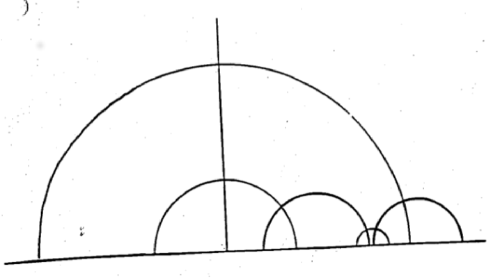
Figure 22: Some h-lines in the upper half-plane

To define a geometry in $U$ we need to define what is meant by a straight line through two points. Given two points $z_{1}$ and $z_{2}$ in $U$, one can construct many circles passing through both of them since three points determine a circle. However, there is a unique circle passing through $z_{1}$ and $z_{2}$ that is perpendicular to $R$. We call this circle the straight line passing through $z_{1}$ and $z_{2}$. When we want to emphasize that we are talking about the hyperbolic line through two points rather than the Euclidean line, we refer to it as an h-line.

You will notice that if $z_{1}$ and $z_{2}$ lie on a vertical line, then there is no Euclidean circle through both that is perpendicular to the boundary. However, recall that a circle on the sphere that passes through the north pole projects onto a what at first glance looks like a line, but is upon reflection can be viewed as a circle (it passes through infinity where it closes up.). We shall also view this line as a circle.

Thus an h-line is either a circle perpendicular to the real axis or a vertical line (see figure  22). (The latter is also automatically perpendicular to the real axis.)

(As a homework exercise you can remind yourself that any circle that intersects the real axis at right angles has its center on the real axis.)

We note that two Euclidean circles are either disjoint, intersect in a point, or intersect in two points. Two circles whose centers are on the real axis that intersect in two points have one point of intersection above the real axis and one below. Thus they have only one point of intersection in the upper half-plane. Similarly, a circle with center on the real axis and a vertical line can have at most one point of intersection in the upper half-plane. Thus any two h-lines are either disjoint or intersect in a point. We have now proved that this system of lines and points satsifies two of the axioms for a geometry.

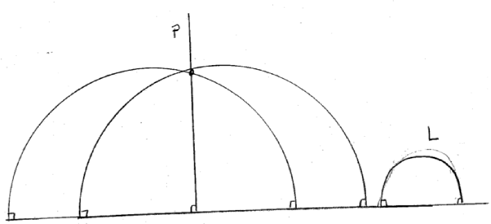
Figure 23: Several h-lines through $p$ that are disjoint from $L$.

35.2 Discussion

• What does a hyperbolic mirror look like?

• What does a hyperbolic mirror string look like?

• What is the maximum number of mirrors in a Euclidean mirror string?

• What is the maximum number of mirrors in a hyperbolic mirror string?

We turn to the parallel axiom. Again let $L$ be any h-line. For the sake of simplicity assume that $L$ is not a vertical h-line. Let $p$ be any point not on $L$. We can construct a whole family of Euclidean circles whose centers are on the real axis which pass through $p$ and which do not intersect $L$. Figure  23 illustrates several such h-lines. For homework, you can work out either one example or a detailed proof.

35.3 Distance

We have emphasized that one of the main distinctions between geometry and topology is that distance is intrinsic to geometry. Thus it behooves us to define a distance in the hyperbolic plane. Again, our emphasis should not be on computing distance, but on having a feel for hyperbolic distance. The important fact to remember is:

• Line segments that appear to be of very different lengths to our Euclidean eyes may be of the same length when we wear hyperbolic glasses and vice-versa.

36 Distance recipe

Here is a technical definition of how to compute distance.

Begin with any two points. If $L$ is the $h$-line on which they lie, let $L^{\prime}$ be the line on the back hemisphere that projects onto $L$. Rotate the sphere so that one of the end points of $L^{\prime}$ moves to the north pole, $N$. $L^{\prime}$ rotates into a new line $L^{\prime\prime}$ passing through $N$. The projection of $L^{\prime\prime}$ is now a vertcal line, $K$. The points $a$ and $b$ have been lifted to $L^{\prime}$ rotated to $L^{\prime\prime}$ and then projected onto $K$. They are now called $a^{\prime}$ and $b^{\prime}$. We can take the ratio of the heights of $a^{\prime}$ and $b^{\prime}$. This is almost a distance. However, distance should be symmetric. The ratio of the heights depends upon which point we name first. Therefore, we take the absolute value of the natural log of the ratio of the heights to be the distance between $a$ and $b$.

36.1 Examples of distances

Consider the two pairs of points

• $A=(0,4)$ and $B=(0,8)$.

• $C=(0,8)$ and $D=(0,16)$.

To our Euclidean eyes it appears to us that $C$ and $D$ are twice as far apart as $A$ and $B$. When we put on our hyperbolic glasses, we realize that the distance between $A$ and $B$ is exactly the same as the distance between $C$ and $D$.

36.2 The Unit Disc Model

Let $D$ be the unit disc in the plane. $D=\{(x,y)|x^{2}+y^{2}<1\}$. We saw earlier that $D$ is the image of the lower half sphere under stereographic projection. This is another model for the hyperbolic plane. We will easily locate the h-lines once we see how this is related to the upper half-plane.

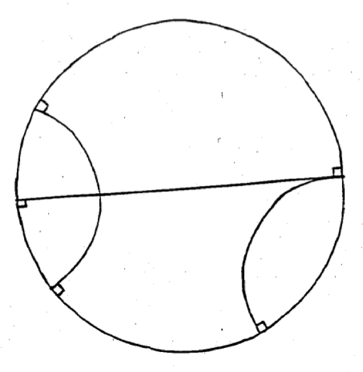
Figure 24: Some h-lines in $D$.

36.3 Passing from one model to another

Take the sphere. Rotate it so that the back hemisphere goes into the bottom hemisphere. Project the bottom hemisphere onto the unit disc. This procedure identifies the upper half plane (the image of the back hemisphere) with the unit disc (the image of the bottom hemisphere). An h-line in the upper half plane corresponds to a circle on the back hemisphere which is perpendicular to the prime meridian. Such a circle rotates into a circle on the bottom hemisphere that is perpendicular to the equator, and then projects to a circle in the plane that intersects the boundary of the unit disc at right angles. When we project onto the unit disc, we no longer have to worry about h-lines through infinity. Things look much more symmetric. However, we still have one weird type of h-line: a Euclidean straight line passing through the center of the disc. (See figure  24.)

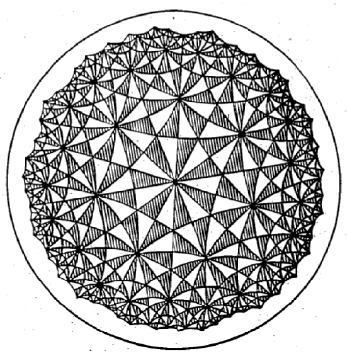
Figure 25: Some hyperbolic cloth: A tiling of the hyperbolic plane by triangles with angles $\pi/2,\pi/3,\hbox{ and }\pi/7$.

Once we have a hyperbolic geometry, many new things are possible.

• We can classify patterns on hyperbolic cloth. We can look for hyperbolic mirrors, hyperbolic gyration points, etc. and analyze hyperbolic cloth just as we analyzed Euclidean cloth.

• We can form a $*237$ orbifold.

Enclosed is a picture of the tiling of the hyperbolic plane by triangles whose angles are $\pi/2$, $\pi/3$ and $\pi/7$. (See figure  25.) The important thing to realize about this picture is that ALL the trianglular tiles are congruent. That is, even though the triangles near the boundary of $D$ appear to be much smaller than those in the center, their sides all have the same lengths. To see this you just have to look through your hyperbolic glasses.

37 A field guide to the orbifolds

The number 17 is just right for the number of types of symmetry patterns in the Euclidean plane: neither too large nor too small. It’s large enough to make learning to recognize them a challenge, but not so large that this is an impossible task. It is by no means necessary to learn to distinguish the 17 types of patterns quickly, but if you learn to do it, it will give you a real feeling of accomplishment, and it is a great way to amaze and overawe your friends, at least if they’re a bunch of nerds and geeks.

In this section, we will give some hints about how to learn to classify the patterns. However, we want to emphasize that this is a tricky business, and the only way to learn it is by hard work. As usual, when you analyze a pattern, you should look first for the mirror strings. The information in this section is meant as a way that you can learn to become more familiar with the 17 types of patterns, in a way that will help you to distinguish between them more quickly, and perhaps in some cases to be able to classify some of the more complicated patterns without seeing clearly and precisely what the quotient is. This kind of superficial knowledge is no substitute for a real visceral understanding of what the quotient orbifold is, and in every case you should go on and try to understand why the pattern is what you say it is while your friends are busy admiring your cleverness.

This information presented in this section has been gleaned from a cryptic manuscript discovered among the personal papers of John Conway after his death. For each of the 17 types of patterns, the manuscript shows a small piece of the pattern, the notation for the quotient orbifold, and Conway’s idiosyncratic pidgin-Greek name for the corresponding pattern. These names are far from standard, and while they are unlikely ever to enter common use, we have found from our own experience that they are not wholly useless as a method for recognizing the patterns.

We will begin by discussing Conway’s names for the orbifolds. A reproduction of Conway’s manuscript appears at the end of the section. You should refer to the reproduction as you try to understand the basis for the names.

37.1 Conway’s names

Each of Conway’s 17 names consists of two parts, a prefix and a descriptor.

37.1.1 The prefix

The prefix tells the number of directions from which you can view the pattern without noticing any difference. The possibilities for the prefix are: hexa-; tetra-; tri-; di-; mono-.

For example, if you are looking at a standard brick wall, it will look essentially the same whether you stand on your feet or on your head. This will be true even if the courses of bricks in the wall do not run parallel to the ground, as they invariably do. Thus you can recognize right away that the brick-wall pattern is di-something-or-other In fact, it is dirhombic.

Another way to think about this is that if you could manage to turn the brick wall upside down, you wouldn’t notice the difference. Again, this would be true even if you kept your head tilted to one side. More to the point, try looking at a dirhombic pattern drawn on a sheet of paper. Place the paper at an arbitrary angle, note what the pattern looks like in the large, and rotate the pattern around until it looks in the large like it did to begin with. When this happens, you will have turned the paper through half a rev. No matter how the pattern is tilted originally, there is always one and only one other direction from which it appear the same in the large.

This ‘in the large’ business means that you are not supposed to notice if, after twisting the paper around, the pattern appears to have been shifted by a translation. You don’t have to go grubbing around looking for some pesky little point about which to rotate the pattern. Just take the wide, relaxed view.

37.1.2 The descriptor

The descriptor represents an attempt on Conway’s part to unite patterns that seem more like each other than they do like the other patterns. The possibilities for the descriptor are: scopic; tropic; gyro; glide; rhombic.

The scopic patterns are those that emerge from kaleidoscopes: $*632=$ hexascopic; $*442=$ tetrascopic; $*333=$ triscopic; $*2222=$ discopic; $**=$ monoscopic;

Their $*$-less counterparts are the tropic patterns (from the Greek for ‘turn’): $632=$ hexatropic; $442=$ tetratropic; $333=$ tritropic; $2222=$ ditropic; $\bullet=$ monotropic.

With the scopic patterns, it’s all done with mirrors, while with the tropic patterns, it’s all done with gyration points. The two exceptions are: $**=$ monoscopic; $\bullet=$ monotropic. There is evidence that Conway did not consider these to be exceptions, on the grounds that ‘with the scopics it’s all done with mirrors and translations, while with the tropics, it’s all done with turnings and translations’.

The gyro patterns contain both mirrors and gyration points: $4*2=$ tetragyro; $3*3=$ trigyro; $22*=$ digyro.

Since both tropic and gyro patterns involve gyration points, there is a real possibility of confusing the names. Strangely, it is the tropic patterns that are the more closely connected to gyration points. In practice, it seems to be easy enough to draw this distinction correctly, probably because the tropics correspond closely to the scopics, and ‘tropic’ rhymes with ‘scopic’. Conway’s view appears to have been that a gyration point, which is a point of rotational symmetry that does NOT lie on a mirror, becomes ever so much more of a gyration point when there are mirrors around that it might have been tempted to lie on, and that therefore patterns that contain both gyration points and mirrors are more gyro than patterns with gyration points but no mirrors.

The glide patterns involve glide-reflections: $22\circ=$ diglide; $\circ\circ=$ monoglide.

The glide patterns are the hardest to recognize. The quotient orbifold of the diglide pattern is a projective plane with two cone points; the quotient of the monoglide patterns is a Klein bottle. When you run up against one of these patterns, you just have to sweat it out. One trick is that when you meet something that has glide-reflections but not much else, then you decide that it must be either a diglide or a monoglide, and you can distinguish between them by deciding whether it’s a di- or a mono- pattern, which is a distinction that is relatively easy to make. Another clue to help distinguish these two cases is that a diglide pattern has glides in two different directions, while a monoglide has glides in only one direction. Yet another clue is that in a monoglide you can often spot two disjoint Möbius strips within the quotient orbifold, corresponding to the fact that the quotient orbifold for a monoglide pattern is a Klein bottle, which can be pieced together from two Möbius strips. These two disjoint Möbius strips arise from the action of glide-reflections along parallel but inequivalent axes.

The rhombic patterns often give a feeling of rhombosity: $2*22=$ dirhombic; $*\circ=$ monorhombic.

An ordinary brick wall is dirhombic; it can be made monorhombic by breaking the gyrational symmetry. The quotient of a monorhombic pattern is a Möbius strip. Like the two glide quotients, it is non-orientable, but it is much easier to identify because of the presence of the mirrors.

37.2 How to learn to recognize the patterns

As you will see, Conway’s manuscript shows only a small portion of each of the patterns. A very worthwhile way of becoming acquainted with the patterns is to draw larger portions of the patterns, and then go through and analyze each one, to see why it has the stated notation and name. You may wish to make flashcards to practice with. When you use these flashcards, you should make sure that you can not only remember the correct notation and name, but also that you can analyze the pattern quickly, locating the distinguishing features. This is important because the patterns you will see in the real world won’t be precisely these ones.

Another hint is to keep your eyes open for symmetrical patterns in the world around you. When you see a pattern, copy it onto a flashcard, even if you cannot analyze it immediately. When you have determined the correct analysis, write it on the back and add it to your deck.

37.3 The manuscript

What follows is an exact reproduction of Conway’s manuscript. In addition to the 17 types of repeating patterns, Conway’s manuscript also gives tables of the 7 types of frieze patterns, and of the 14 types of symmetrical patterns on the sphere. These parts of the manuscript appear to be mainly gibberish. We reproduce these tables here in the hope that they may someday come to the attention of a scholar who will be able to make sense of them.