Zero-Temperature Limit and Statistical Quasiparticles in Many-Body Perturbation Theory

Abstract

The order-by-order renormalization of the self-consistent mean-field potential in many-body perturbation theory for normal Fermi systems is investigated in detail. Building on previous work mainly by Balian and de Dominicis, as a key result we derive a thermodynamic perturbation series that manifests the consistency of the adiabatic zero-temperature formalism with perturbative statistical mechanics—for both isotropic and anisotropic systems—and satisfies at each order and for all temperatures the thermodynamic relations associated with Fermi-liquid theory. These properties are proved to all orders.

I Introduction

Many-body perturbation theory (MBPT) represents the elementary framework for calculations aimed at the properties of nonrelativistic many-fermion systems at zero and finite temperature. In general, for Fermi systems the correct ground-state is not a normal state but involves Cooper pairs Luttinger (1966); Kohn and Luttinger (1965); Baranov et al. (1992); Shankar (1994); Salmhofer (1999). However, pairing effects can often be neglected for approximative calculations of thermodynamic properties close to zero temperature. For such calculations there are two formalisms: first, there is grand-canonical perturbation theory, and second, the zero-temperature formalism based on the adiabatic continuation of the ground state Gell-Mann and Low (1951); Goldstone (1957); Nozières (1964); Gross and Runge (1986); Negele and Orland (1998); Fetter and Walecka (1972); Abrikosov et al. (1975). In their time-dependent (i.e., in frequency space) formulations, these two formalisms give matching results if all quantities are derived from the exact Green’s functions, i.e., from the self-consistently renormalized propagators Luttinger and Ward (1960); Fetter and Walecka (1972); Abrikosov et al. (1975); Feldman et al. (1999). The renormalization of MBPT in frequency space can be generalized to vertex functions de Dominicis and Martin (1964a, b); Haussmann (1999); Rossi and Werner (2015); Rossi et al. (2016); Dickhoff and Barbieri (2004); Van Houcke et al. (2012), and is essential to obtain a fully consistent framework for calculating transport properties Baym and Kadanoff (1961); Baym (1962); Stefanucci and van Leeuwen (2003).

Nevertheless, the use of bare propagators has the benefit that in that case the time integrals can be performed analytically. With bare propagators, MBPT in its most basic form corresponds to a perturbative expansion in terms of the interaction Hamiltonian $V$ about the noninteracting system with Hamiltonian $H_{0}$, where $H=H_{0}+V$ is the full Hamiltonian. First-order self-energy effects can be included to all orders in bare MBPT by expanding instead about a reference Hamiltonian $H_{\text{ref}}=H_{0}+U_{1}$, where $U_{1}$ includes the first-order contribution to the (frequency-space) self-energy $\Sigma_{1,{\textbf{k}}}$ as a self-consistent single-particle potential (mean field). The renormalization of $H_{\text{ref}}$ in terms of $U_{1}$ has the effect that all two-particle reducible diagrams with first-order pieces (single-vertex loops) are canceled. At second order the self-energy becomes frequency dependent and complex, so the equivalence between the propagator renormalization in frequency space and the renormalization of the mean-field part of $H_{\text{ref}}$ in bare MBPT is restricted to the Hartree-Fock level.

Zero-temperature MBPT calculations with bare propagators and a Hartree-Fock reference Hamiltonian ${H_{\text{ref}}=H_{0}+U_{1}}$ are common in quantum chemistry and nuclear physics. With a Hartree-Fock reference Hamiltonian (or, with ${H_{\text{ref}}=H_{0}}$), however, the adiabatic zero-temperature formalism is inconsistent with the zero-temperature limit (${T\rightarrow 0}$) of grand-canonical MBPT. The (main) fault however lies not with zero-temperature MBPT, but with the grand-canonical perturbation series: in the bare grand-canonical formalism (with $H_{\text{ref}}\in\{H_{0},H_{0}+U_{1}\}$) there is a mismatch in the Fermi-Dirac distribution functions caused by using the reference spectrum $\varepsilon_{\textbf{k}}$ together with the true chemical potential $\mu$, and in general this leads to deficient results Fritsch et al. (2002); Wellenhofer et al. (2014); Wellenhofer (2017). The adiabatic formalism on the other hand uses the reference chemical potential, i.e., the reference Fermi energy $\varepsilon_{\text{F}}$. Related to this is the presence of additional contributions from two-particle reducible diagrams, the so-called anomalous contributions, in the grand-canonical formalism.

This issue is usually dealt with by modifying the grand-canonical perturbation series for the free energy in terms of an expansion about the chemical potential $\mu_{\text{ref}}\xrightarrow{T\rightarrow 0}\varepsilon_{\text{F}}$ of the reference system Kohn and Luttinger (1960); Brout and Englert (1960) (see also Sec. IV.2). This expansion introduces additional anomalous contributions, and for isotropic systems these can be seen to cancel the old ones for ${T\rightarrow 0}$ Luttinger and Ward (1960). Thus, the modified perturbation series for the free energy $F(T,\mu_{\text{ref}})$ reproduces the adiabatic series in the isotropic case. For anisotropic systems, however, the anomalous contributions persist at ${T=0}$ (for ${H_{\text{ref}}=H_{0}+U_{1}}$, at fourth order and beyond). Negele and Orland Negele and Orland (1998) interpret this feature as follows: there is nothing fundamentally wrong with the bare zero-temperature formalism, but for anisotropic systems the adiabatic continuation must be based on a better reference Hamiltonian $H_{\text{ref}}$. Since the convergence rate of MBPT depends on the choice of $H_{\text{ref}}$, this issue is relevant also for finite-temperature calculations, and for isotropic systems.

Recently, Holt and Kaiser Holt and Kaiser (2017) have shown that including the real part of the bare second-order contribution to the (on-shell) self-energy, $\text{Re}\,[\Sigma_{2,{\textbf{k}}}(\varepsilon_{\textbf{k}})]$, as the second-order contribution to the self-consistent mean field has a significant effect in perturbative nuclear matter calculations with modern two- and three-nucleon potentials (see, e.g., Refs. Epelbaum et al. (2009); Machleidt and Entem (2011); Bogner et al. (2010)). However, a formal clarification for the renormalization of $H_{\text{ref}}$ in terms of $\text{Re}\,[\Sigma_{2,{\textbf{k}}}(\varepsilon_{\textbf{k}})]$ was not included in Ref. Holt and Kaiser (2017). In particular, from the discussion of Ref. Holt and Kaiser (2017) it is not clear whether the use of this second-order mean field should be considered an improvement or not, compared to calculations with a Hartree-Fock mean field.

A general scheme where the reference Hamiltonian is renormalized at each order in grand-canonical MBPT was introduced by Balian, Bloch, and de Dominicis Balian et al. (1961a) (see also Refs. Balian et al. (1961b); Balian and de Dominicis (1964); Bloch (1960, 1965); de Dominicis (1964)). This scheme however leads to a mean field whose functional form is given by $U[n_{\textbf{k}},T]$, where $n_{\textbf{k}}(T,\mu)$ is the Fermi-Dirac distribution and the explicit temperature dependence involves factors $\operatorname{\operatorname{e}}^{\pm(\varepsilon_{\textbf{k}}-\mu)/T}$. Because of the $\operatorname{\operatorname{e}}^{\pm(\varepsilon_{\textbf{k}}-\mu)/T}$ factors, the resulting perturbation series is well-behaved only at sufficiently large temperatures, and its ${T\rightarrow 0}$ limit does not exist.

A different renormalization scheme was outlined by Balian and de Dominicis (BdD) in Refs. Balian and de Dominicis (1960); de Dominicis (1960) (see also Refs. de Dominicis (1964); Bloch (1965)). At second order, this scheme leads to the mean field employed by Holt and Kaiser Holt and Kaiser (2017). The outline given in Refs. Balian and de Dominicis (1960); de Dominicis (1960) indicates the following results:

1. The functional form of the mean field is to all orders given by $U[n_{\textbf{k}}]$, i.e., there is no explicit temperature dependence (apart from the one given by the Fermi-Dirac distributions), so the ${T\rightarrow 0}$ limit exists.

2. The zero-temperature limit of the renormalized grand-canonical perturbation series for the free energy $F(T,\mu)$ reproduces the (correspondingly renormalized) adiabatic series for the ground-state energy $E^{(0)}(\varepsilon_{\text{F}})$ to all orders; i.e., the reference spectrum $\varepsilon_{\textbf{k}}$ has been adjusted to the true chemical potential $\mu$, with $\varepsilon_{\text{F}}=\mu$ at ${T=0}$.

3. One obtains at each perturbative order and for all temperatures the thermodynamic relations associated with Fermi-liquid theory Landau (1957a). This result corresponds to the notion statistical quasiparticles Pethick and Carneiro (1973); Carneiro and Pethick (1975); Baym and Pethick (1991).

The most intricate part in establishing these results is as follows. For ${T\neq 0}$, there are no energy denominator poles in the (proper) expressions for the perturbative contributions to the grand-canonical potential. The BdD renormalization scheme however introduces such poles, and therefore a regularization procedure is required to apply the scheme. So far, this issue has been studied in more detail only for the case of impurity systems Balian and de Dominicis (1971); Luttinger and Liu (1973); Keiter and Morandi (1984).

Motivated by this situation, in the present paper we revisit the order-by-order renormalization of the reference Hamiltonian in bare MBPT. First, in Sec. II we give a short review of grand-canonical perturbation theory with bare propagators and introduce the various order-by-order renormalizations of the reference Hamiltonian. We also discuss how dynamical quasiparticles arise in (frequency-space) MBPT, and show that their energies are distinguished from the ones of the statistical quasiparticles associated with result (2). In Sec. III we discuss the regularization procedure for the BdD renormalization scheme, and analyze the resulting expressions for the second- and third-order contributions to the grand-canonical potential and the BdD mean field. In Sec. IV we prove to all orders that the BdD renormalized perturbation series satisfies the Fermi-liquid relations (2) and, as a consequence, manifests the consistency of the adiabatic zero-temperature formalism (1). The paper is concluded in Sec. V. In Appendix A, we derive explicitly the renormalized contribution from two-particle reducible diagrams at fourth order. In Appendix B, we discuss in more detail the various forms of the self-energy, derive various expressions for the mean occupation numbers, and examine the functional relations between the grand-canonical potential and the (various forms of the) self-energy in bare MBPT.

II Grand-Canonical Perturbation Theory

II.1 Setup

We consider a homogeneous but not necessarily isotropic system of nonrelativistic fermions in thermodynamic equilibrium. The Hamiltonian is given by ${H=H_{0}+V}$, where $V$ is a two-body operator representing pair interactions. Multi-fermion interactions do not raise any new formal or conceptual issues, and are therefore neglected. For notational simplicity and without loss of generality we assume a single species of spinless fermions. If there is no external potential, then $H_{0}$ is the kinetic energy operator. We now introduce an additional one-body operator $U$, and write

$$H=\underbrace{(H_{0}+U)}_{H_{\text{ref}}}+(V-U).$$ (1)

The operator $U$ represents a mean field, i.e., an effective one-body potential which allows to define a solvable reference system that includes the effects of pair interactions in the system to a certain degree. For a homogeneous system the mean field should preserve translational invariance, so the eigenstates $\ket{\psi_{\textbf{k}}}$ of the momentum operator are eigenstates of $H_{\text{ref}}=H_{0}+U$, i.e.,

$$H_{\text{ref}}\ket{\psi_{\textbf{k}}}=\varepsilon_{\textbf{k}}\ket{\psi_{\textbf{k}}}.$$ (2)

Because the mean field is supposed to include interaction effects self-consistently, the single-particle energies $\varepsilon_{\textbf{k}}$ are determined by the self-consistent equation

$$\varepsilon_{\textbf{k}}=\varepsilon_{0,\textbf{k}}+U_{\textbf{k}}[\varepsilon_{\textbf{k}}],$$ (3)

where $\varepsilon_{0,\textbf{k}}=\braket{\psi_{\textbf{k}}}{H_{0}}{\psi_{\textbf{k}}}$ and $U_{\textbf{k}}[\varepsilon_{\textbf{k}}]=\braket{\psi_{\textbf{k}}}{U}{\psi_{\textbf{k}}}$. The occupation number representation of the reference Hamiltonian $H_{\text{ref}}=H_{0}+U$ is then given by

$$\mathcal{H}_{\text{ref}} =\sum_{\textbf{k}}\braket{\psi_{\textbf{k}}}{H_{\text{ref}}}{\psi_{\textbf{k}}}a^{\dagger}_{\textbf{k}}a_{\textbf{k}},$$ (4)

where $a^{\dagger}_{\textbf{k}}$ and $a_{\textbf{k}}$ are creation and annihiliation operators with respect to momentum eigenstates. If not indicated explicitly otherwise, we assume the thermodynamic limit where $\sum_{\textbf{k}}\rightarrow\int\!d^{3}k/(2\pi)^{3}$. The occupation number representation of the perturbation Hamiltonian ${H-H_{\text{ref}}=V-U}$ is given by

$$\mathcal{V} =\frac{1}{2!}\sum_{\textbf{k}_{1},\textbf{k}_{2},\textbf{k}_{3},\textbf{k}_{4}}\braket{\psi_{\textbf{k}_{1}}\psi_{\textbf{k}_{2}}}{V}{\psi_{\textbf{k}_{3}}\psi_{\textbf{k}_{4}}}a^{\dagger}_{\textbf{k}_{1}}a^{\dagger}_{\textbf{k}_{2}}a_{\textbf{k}_{4}}a_{\textbf{k}_{3}}$$

$$\quad-\sum_{\textbf{k}}\braket{\psi_{\textbf{k}}}{U}{\psi_{\textbf{k}}}a^{\dagger}_{\textbf{k}}a_{\textbf{k}},$$ (5)

where momentum conservation is implied, i.e., $\textbf{k}_{1}+\textbf{k}_{2}$$=\textbf{k}_{3}+\textbf{k}_{4}$. We assume that the potential $V$ is sufficiently regular(ized) such that no ultraviolet Hammer and Furnstahl (2000); Wellenhofer et al. (2018) or infrared Gell-Mann and Brueckner (1957) divergences appear in perturbation theory. Further, we require that $V$ has a form (e.g., finite-rangedinteractions) for which the thermodynamic limit exists; see, e.g., Refs. Haag (1996); D. Ruelle (1969); Lieb and Seiringer (2010).

II.2 Perturbation series and diagrammatic analysis

II.2.1 Grand-canonical perturbation series

For truncation order $N$, the perturbation series for the grand-canonical potential $\Omega(T,\mu)$ is given by

$$\Omega(T,\mu)=\Omega_{\text{ref}}(T,\mu)+\Omega_{U}(T,\mu)+\sum_{n=1}^{N}\Omega_{n}(T,\mu),$$ (6)

where

$$\Omega_{\text{ref}}(T,\mu) =T\sum_{\textbf{k}}\ln(\bar{n}_{\textbf{k}}),$$

$$\Omega_{U}(T,\mu) =-\sum_{\textbf{k}}U_{\textbf{k}}n_{\textbf{k}}.$$ (7)

Here, $\bar{n}_{\textbf{k}}=1-n_{\textbf{k}}$, with $n_{\textbf{k}}=[1+\operatorname{\operatorname{e}}^{\beta(\varepsilon_{\textbf{k}}-\mu}]^{-1}$ the Fermi-Dirac distribution function, and $\beta=1/T$. From the grand-canonical version of Wick’s theorem one obtains the following formula Fetter and Walecka (1972); Bloch and de Dominicis (1958) for $\Omega_{n}(T,\mu)$:

$$\Omega_{n}^{\text{direct}[P]}=-\frac{1}{\beta}\frac{(-1)^{n}}{n!}\int\limits_{0}^{\beta}\!d\tau_{n}\cdots d\tau_{1}\;\Braket{\mathcal{T}\big{[}\mathcal{V}(\tau_{n})\cdots\mathcal{V}(\tau_{1})\big{]}}_{L},$$ (8)

where $\mathcal{T}$ is the time-ordering operator and $\mathcal{V}(\tau)=\operatorname{\operatorname{e}}^{\mathcal{H}_{\text{ref}}\tau}\mathcal{V}\operatorname{\operatorname{e}}^{-\mathcal{H}_{\text{ref}}\tau}$ is the interaction picture representation (in imaginary time) of the perturbation operator $\mathcal{V}$ given by Eq. (II.1).

II.2.2 Classification of diagrams

The various ways the Wick contractions in the unperturbed ensemble average $\braket{\ldots}$ can be performed can be represented by Hugenholtz diagrams, i.e., diagrams composed of $V$ and $-U$ vertices, and directed lines attached to vertices at both ends. Left-pointing lines are called holes and correspond to factors $n_{\textbf{k}}$, right-pointing lines are called particles and have factors $\bar{n}_{\textbf{k}}$. In the case of two-particle reducible diagrams, momentum conservation implies that there are two or more lines with identical three-momenta. We refer to these lines as articulation lines. The diagrammatic parts connected via articulation lines are referred to as pieces. Two-particle irreducible diagrams have only $V$ vertices. Two-particle reducible diagrams where at least one set of lines with identical three-momenta includes both holes and particles are called anomalous, with the indicative lines referred to as anomalous articulation lines. All other (two-particle reducible or irreducible) diagrams are called normal. The parts of anomalous diagrams connected via anomalous articulation lines are called normal pieces. In general, normal two-particle reducible diagrams transform into anomalous diagrams under vertex permutations, see Figs. 3, 5 and 6.

In Eq. (8), the subscript $L$ means that only linked diagrams are taken into account. By virtue of the time integration and the time-ordering operator, in Eq. (8) there is no distinction between diagrams connected via vertex permutations; in particular, there is no distinction between normal and anomalous two-particle reducible diagrams. The distinction between the different diagrams in the permutation invariant sets of diagrams is however relevant for the time-independent formulas discussed below.

II.2.3 Time-independent formulas

From Eq. (8), Bloch and de Dominicis Bloch and de Dominicis (1958) (see also Refs. Bloch (1961, 1965); Keiter and Morandi (1984)) have derived several time-independent formulas for $\Omega_{n}(T,\mu)$. One of them, here referred to as the direct formula, is given by

$$\Omega_{n}^{\text{direct}} =\frac{1}{\beta}\frac{(-1)^{n}}{2\pi\text{i}}\oint_{C}dz\frac{\operatorname{\operatorname{e}}^{-\beta z}}{z^{2}}\Braket{\mathcal{V}\frac{1}{D_{n}-z}\cdots\mathcal{V}\frac{1}{D_{1}-z}\mathcal{V}}_{\!L},$$ (9)

where the contour $C$ encloses all the poles ${z=0,D_{1},\ldots,D_{n}}$, with $D_{\nu\in\{1,\ldots,n\}}$ the energy denominators for the respective diagrams. Furthermore, in Eq. (9), it is implied that the contributions from all poles are summed before the momentum integration, i.e., the $z$ integral is performed inside the momentum integrals. This has the consequence that the integrands of the momentum integrals have no poles (for ${T\neq 0}$, see below) from vanishing energy denominators. The expressions obtained from the direct formula deviate from the ones obtained from the time-dependent formula Eq. (8), but—as evident from the derivation of direct formula Bloch and de Dominicis (1958)—the sum of the direct expressions obtained for a set of diagrams that is closed under vertex permutations is equivalent (but not identical) to the expression obtained from Eq. (8).

From the cyclic property of the trace, another time-independent formula can be derived Bloch and de Dominicis (1958), here referred to as the cyclic formula, i.e.,

$$\Omega_{n}^{\text{cyclic}} =\frac{1}{n}\frac{(-1)^{n+1}}{2\pi\text{i}}\oint_{C}dz\frac{\operatorname{\operatorname{e}}^{-\beta z}}{z}\Braket{\mathcal{V}\frac{1}{D_{n}-z}\cdots\mathcal{V}\frac{1}{D_{1}-z}\mathcal{V}}_{\!L},$$ (10)

where again it is implied that the $z$ integral is performed inside the momentum integrals; again, this has the consequence that the integrands have no poles (for ${T\neq 0}$). The direct and the cyclic formula give equivalent (but not identical) expressions only for the sums of diagrams connected via cyclic vertex permutations, and the cyclic expressions for the individual diagrams in these cyclic groups are equivalent.

Finally, from the analysis of the contributions from the different poles in Eq. (10) one can formally write down a reduced form of the cyclic formula Bloch and de Dominicis (1958), here referred to as the reduced formula, i.e.,

$$\Omega_{n}^{\text{reduced}} =\frac{(-1)^{n+1}}{\mathcal{O}}\underset{z=0}{\text{Res}}\frac{\operatorname{\operatorname{e}}^{-\beta z}}{z}\Braket{\mathcal{V}\frac{1}{D_{n}-z}\cdots\mathcal{V}\frac{1}{D_{1}-z}\mathcal{V}}_{\!L},$$ (11)

where $\mathcal{O}$ is the order of the pole at $z=0$. The reduced expressions for normal diagrams are identical to the usual expressions of zero-temperature MBPT, except that the step functions are replaced by Fermi-Dirac distributions. As a consequence, while at ${T=0}$ the energy denominator poles in these expressions are at the integration boundary, for ${T\neq 0}$ they are in the interior. This entails that the reduced expressions for individual diagrams are not well-defined for ${T\neq 0}$.

Last, we note that each of the time-independent formulas can be applied also to unlinked diagrams (the only change being the omission of the subscript $L$); this will become relevant in Sec. IV.

II.2.4 Classification of perturbative contributions

Anomalous diagrams give no contribution in zero-temperature MBPT. However, the contributions from anomalous diagrams in grand-canonical MBPT do not vanish for ${T\rightarrow 0}$ (in the thermodynamic limit). The reduced integrands (which are well-defined at ${T=0}$) for diagrams with identically vanishing energy denominators have terms of the form

$$\frac{\partial^{\nu}n_{\textbf{k}}}{\partial\mu^{\nu}}\xrightarrow{T\rightarrow 0}\delta^{(\nu)}(\mu-\varepsilon_{\textbf{k}}),$$ (12)

e.g., $\beta n_{\textbf{k}}\bar{n}_{\textbf{k}}=\partial n_{\textbf{k}}/\partial\mu\xrightarrow{T\rightarrow 0}\delta(\mu-\varepsilon_{\textbf{k}})$. Contributions with such terms are called anomalous contributions. There are also contributions that vanish for ${T\rightarrow 0}$, e.g.,

$$n_{\textbf{k}}\bar{n}_{\textbf{k}}=T\frac{\partial n_{\textbf{k}}}{\partial\mu}\xrightarrow{T\rightarrow 0}0.$$ (13)

Such pseudoanomalous contributions can be associated also with normal two-particle reducible diagrams via the relation

$$\bar{n}_{\textbf{k}}=1-n_{\textbf{k}},$$ (14)

i.e.,

$$n_{\textbf{k}}n_{\textbf{k}} =n_{\textbf{k}}-n_{\textbf{k}}\bar{n}_{\textbf{k}},$$ (15)

$$\bar{n}_{\textbf{k}}\bar{n}_{\textbf{k}} =\bar{n}_{\textbf{k}}-n_{\textbf{k}}\bar{n}_{\textbf{k}},$$ (16)

$$n_{\textbf{k}}n_{\textbf{k}}n_{\textbf{k}} =n_{\textbf{k}}-2n_{\textbf{k}}\bar{n}_{\textbf{k}}+n_{\textbf{k}}\bar{n}_{\textbf{k}}\bar{n}_{\textbf{k}},$$ (17)

$$\bar{n}_{\textbf{k}}\bar{n}_{\textbf{k}}\bar{n}_{\textbf{k}} =\bar{n}_{\textbf{k}}-2n_{\textbf{k}}\bar{n}_{\textbf{k}}+n_{\textbf{k}}n_{\textbf{k}}\bar{n}_{\textbf{k}},$$ (18)

etc. Contributions which are not anomalous or pseudoanomalous are referred to as normal contributions. Following loosely Balian, Bloch, and de Dominicis Balian et al. (1961a), we refer to the application of Eq. (14) according to Eqs. (15)–(18), etc. as disentanglement, denoted symbolically by $\div$.

For the ${T\rightarrow 0}$ limit, the energy denominator exponentials present in the direct and cyclic formula all have to be evaluated via

$$\bar{n}_{\textbf{k}}\operatorname{\operatorname{e}}^{-\beta(\varepsilon_{\textbf{k}}-\mu)}=n_{\textbf{k}}.$$ (19)

The simple relations given by Eqs. (14) and (19) play a crucial role in many of the issues and results discussed in the present paper.

II.3 Discrete spectrum inconsistency and anomalous contributions

Apart from being essential for practical many-body calculations, the thermodynamic limit is in fact essential for the thermodynamic consistency of the grand-canonical perturbation series at low $T$, in particular for ${T\rightarrow 0}$, in the general case (see below). For a finite system with a discrete spectrum at ${T=0}$ one has either $\mu\in\{\varepsilon_{\textbf{k}}\}$ or $\mu\not\in\{\varepsilon_{\textbf{k}}\}$. Both cases are inconsistent.

In the first case the ${T\rightarrow 0}$ limit is singular, because in that case the anomalous contributions diverge. In addition, for discrete systems and $\mu\in\{\varepsilon_{\textbf{k}}\}$ the ${T\rightarrow 0}$ limit is singular due to energy denominator singularities.

In the second case the anomalous contributions vanish for ${T\rightarrow 0}$. From $F(T,\mu)=\Omega(T,\mu)+\mu\varrho(T,\mu)$ and the fact that all contributions to $\varrho(T,\mu)=-\partial\Omega(T,\mu)/\partial\mu$ except the ones from $\Omega_{\text{ref}}(T,\mu)$ are anomalous, for $\mu\not\in\{\varepsilon_{\textbf{k}}\}$ we obtain

$$F(T,\mu)\xrightarrow{T\rightarrow 0}E^{(0)}(\mu),\;\;\;\;\;\;\;\;\;\;\varrho(T,\mu)\xrightarrow{T\rightarrow 0}\sum_{\textbf{k}}\theta(\mu-\varepsilon_{\textbf{k}}),$$ (20)

where $E^{(0)}(\varepsilon_{\text{F}})$ corresponds to the adiabatic series. As noted by Kohn and Luttinger Kohn and Luttinger (1960), the two parts of Eq. (20) are inconsistent with each other. A possible definition of the chemical potential at ${T=0}$ in the finite case is

$$\mu(T=0,\varrho)=\frac{E^{(0)}(\varrho+1)+E^{(0)}(\varrho)}{2}.$$ (21)

The second part of Eq. (20) however is equivalent to

$$\mu(T=0,\varrho)=\frac{E_{\text{ref}}^{(0)}(\varrho+1)+E_{\text{ref}}^{(0)}(\varrho)}{2}\equiv\mu_{\text{ref}}(T=0,\varrho),$$ (22)

which contradicts the previous equation. For a given particle number the true chemical potential deviates from the chemical potential of the reference system, and Eq. (20) would imply that they are equal at $T=0$. Thus, in the discrete case the ${T\rightarrow 0}$ limit of the grand-canonical perturbation series is inconsistent also for $\mu\not\in\{\varepsilon_{\textbf{k}}\}$.

The same inconsistency can arise in the thermodynamic limit if the reference spectrum has a gap $\Delta$ and $\mu\not\in\{\varepsilon_{\textbf{k}}\}$. The ${T\rightarrow 0}$ limit is still smooth in the discrete (gapped) case, so the inconsistency is still present for nonzero $T$, although it is washed out at sufficiently high $T$. Qualitatively, in the discrete case the inconsistency is relevant if the spectrum does not resolve the anomalous terms $\partial^{\nu}n_{\textbf{k}}/\partial\mu^{\nu}$. As discussed in Sec. II.4, contributions with such terms can be seen to account for the mismatch generated by using the reference spectrum together with the true chemical potential. If the anomalous terms are not sufficiently resolved the information about this mismatch gets lost and one approaches the paradoxical result that $\mu(T,\varrho)=\mu_{\text{ref}}(T,\varrho)$.

There are two ways the discrete (gapped) spectrum inconsistency for $\mu\not\in\{\varepsilon_{\textbf{k}}\}$ can be partially resolved, i.e.,

1. by using the reference chemical potential instead of the true one,

2. by choosing a mean-field that leads to $\mu({T=0},\varrho)=\mu_{\text{ref}}({T=0},\varrho)$.

Case (i) corresponds to the modified perturbation series $F(T,\mu_{\text{ref}})$. The partial resolution of the discrete spectrum inconsistency in that case is as follows:

1. $F(T,\mu_{\text{ref}})$ involves additional anomalous contributions, and the failure to resolve the old ones is balanced (for anisotropic systems, only partially) by not resolving the new ones.

In the gapped case $F(T,\mu_{\text{ref}})$ reproduces the adiabatic series in the ${T\rightarrow 0}$ limit (if $\mu_{\text{ref}}\not\in\{\varepsilon_{\textbf{k}}\}$). In the gapless case the adiabatic series is reproduced only for isotropic systems; in that case the old and new anomalous contributions cancel for ${T\rightarrow 0}$. Thus, there is still a remainder of the discrete spectrum inconsistency. The information about anisotropy encoded in the anomalous contributions is not resolved in the discrete case at low $T$. In particular, for $F(T,\mu_{\text{ref}})$ the thermodynamic limit (and ${\Delta\rightarrow 0}$ limit, respectively) and the ${T\rightarrow 0}$ limit are noncommuting limits in the anisotropic case.

Regarding case (ii), there are three mean-field renormalization schemes that lead to $\mu(T,\varrho)=\mu_{\text{ref}}(T,\varrho)$, and accordingly, $F(T,\mu)=F(T,\mu_{\text{ref}})$: the direct, the cyclic, and the BdD scheme; see Sec. II.4. The anomalous diagrams are removed in each scheme, but in the direct and cyclic schemes there are still anomalous contributions. Hence, for the direct and cyclic schemes there is no discrete spectrum inconsistency despite anomalous contributions. However, these schemes are well-behaved only at high $T$ where the inconsistency ceases to be relevant. In particular, the ${T\rightarrow 0}$ limit does not exist for the direct and cyclic scheme.

The ${T\rightarrow 0}$ limit exists for the BdD scheme, but for ${N>2}$ this scheme exists only in the thermodynamic limit. The commutativity of the ${T\rightarrow 0}$ and ${\Delta\rightarrow 0}$ limits is fully restored in the BdD scheme, irrespective of isotropy. The anomalous contributions can be removed and the result $\mu({T=0},\varrho)=\mu_{\text{ref}}({T=0},\varrho)$ can be achieved also for finite systems, via the mean-field renormalization scheme specified by Eq. (48) below. For ${N\leq 2}$ the Eq. (48) scheme converges to the BdD scheme, but for ${N>2}$ it becomes ill-defined (singular, for ${N\geq 4}$) in the thermodynamic limit. Altogether, we have:

1. The result $\mu({T=0},\varrho)=\mu_{\text{ref}}({T=0},\varrho)$ can be achieved for finite systems and in the thermodynamic limit, irrespective of isotropy, but for ${N>2}$ these two cases are not smoothly connected.

The commutativity of limits can however be fully restored for $F(T,\mu_{\text{ref}})$:

1. For $F(T,\mu_{\text{ref}})$ together with the mean-field renormalization scheme given by Eq. 153 below the limit ${T\rightarrow 0}$ commutes with both the thermodynamic limit and the ${\Delta\rightarrow 0}$ limit, irrespective of isotropy. This is because for $F(T,\mu_{\text{ref}})$, at ${T=0}$ the Eq. 153 scheme removes the anomalous contributions.

Case (ii) and case (iii) both lead to the adiabatic formalism, irrespective of isotropy. There are however still anomalous contributions at finite $T$ in case (iii), and the reference chemical potential is identified with the true chemical potential only in case (ii).

II.4 Mean-field renormalization schemes

The usual choices for the mean-field potential are ${U=0}$ (free reference spectrum) or ${U=U_{1}}$ (Hartree-Fock spectrum). In general, one expects that the choice ${U=U_{1}}$ leads to an improved perturbation series, compared to ${U=0}$. For first-order MBPT this can be seen from the fact that ${U=U_{1}(T,\mu)}$ and ${U=U_{1}(\varepsilon_{\text{F}})}$, respectively, are stationary points of the right-hand sides of the inequalities

$$\Omega(T,\mu) \leq\Omega_{\text{ref}}(T,\mu)+\Omega_{U}(T,\mu)+\Omega_{1}(T,\mu),$$ (23)

$$E^{(0)}(\varepsilon_{\text{F}}) \leq E^{(0)}_{\text{ref}}(\varepsilon_{\text{F}})+E^{(0)}_{U}(\varepsilon_{\text{F}})+E^{(0)}_{1}(\varepsilon_{\text{F}}),$$ (24)

for grand-canonical and adiabatic MBPT, respectively. For truncation orders $N>1$, however, no similar formal argument is available for ${U=U_{1}}$ representing the best choice.

For both ${U=0}$ and ${U=U_{1}}$, in the thermodynamic limit the grand-canonical perturbation series does not reproduce the adiabatic one for $T\rightarrow 0$. The adiabatic series is also not reproduced in the discrete case, and in that case the grand-canonical series is inconsistent, in general (in particular, for ${U\in\{\,0,U_{1}\}}$); see Sec. II.3).

It is now important to note that, at least for ${U=0}$, in general bare grand-canonical MBPT leads to deficient results also in the thermodynamic limit. This is particularly evident for a system with a first-order phase transition: for ${U=0}$ it is impossible to obtain the nonconvex single-phase constrained free energy from $\Omega(T,\mu)$, since $\Omega(T,\mu)$ is necessarily a single-valued function of $\mu$ for ${U=0}$; see also Refs. Fritsch et al. (2002); Wellenhofer et al. (2014); Wellenhofer (2017).

This deficiency can be repaired by modifying the expression for $F(T,\mu)$ in terms of a (truncated) formal expansion about the chemical potential $\mu_{\text{ref}}\xrightarrow{T\rightarrow 0}\varepsilon_{\text{F}}$ of the reference system; see Sec. IV.2 for details. This expansion introduces additional contributions, and the structure of these contributions is very similar to anomalous diagrams. For isotropic systems it can be seen that the anomalous parts of these additional contributions cancel the old ones for ${T\rightarrow 0}$, leading to

$$F(T,\mu_{\text{ref}})\xrightarrow{T\rightarrow 0}E^{(0)}(\varepsilon_{\text{F}})$$ (25)

in the isotropic case.

For $\Omega(T,\mu)$ with ${U=U_{1}(T,\mu)}$ one has $\varrho(T,\mu)=\sum_{\textbf{k}}n_{\textbf{k}}$ at truncation order ${N=1}$. Thus, for ${N=1}$ (but not for ${N>1}$) it is

$$F(T,\mu)=F(T,\mu_{\text{ref}}),$$ (26)

with $\mu(T,\varrho)=\mu_{\text{ref}}(T,\varrho)$, where $F(T,\mu_{\text{ref}})$ now corresponds to the modified series with ${U=U_{1}(T,\mu_{\text{ref}})}$. For $\Omega(T,\mu)$ the change from ${U=0}$ to ${U=U_{1}}$ removes all anomalous (and normal) diagrams with single-vertex loops. For $F(T,\mu_{\text{ref}})$ both the reference spectrum and the reference chemical potential get renormalized, and both the anomalous diagrams and the additional ones with single-vertex loops are removed.

Now, these features make evident that there is a deficiency in the grand-canonical series with ${U=0}$ irrespective of the presence of a first-order phase transition: there is a mismatch in the Fermi-Dirac distribution functions generated by using the spectrum of $H_{0}$ together with the true chemical potential, leading to decreased perturbative convergence, compared to $F(T,\mu_{\text{ref}})$ with the same setup. One may interpret the anomalous contributions as a symptom of this mismatch. In that sense, the “expanding away” of the mismatch, i.e., the construction of $F(T,\mu_{\text{ref}})$, corresponds to a symptomatic treatment that provides as remedy additional anomalous contributions that counteract the old ones. The mismatch can however be ameliorated (cured, for $N=1$, in the $U=U_{1}$ case) by improving the quality of the reference Hamiltonian: the change from ${U=0}$ to ${U=U_{1}}$ removes the main symptom (and the corresponding remedy, in the modified case), the anomalous diagrams with single-vertex loops.

Altogether, this suggests that one can expect that the convergence behavior of $\Omega(T,\mu)$ is inferior to the one of $F(T,\mu_{\text{ref}})$ also for ${U=U_{1}}$. Moreover, one can suspect that both $\Omega(T,\mu)$ and $F(T,\mu_{\text{ref}})$ may be further improved by using a mean field beyond Hartree-Fock. In the best case, the additional mean-field contributions should remove all the remaining anomalous diagrams (and additional diagrams, for the modified series), i.e., the ones with higher-order pieces, and lead to $F(T,\mu)=F(T,\mu_{\text{ref}})$ for truncation orders ${N>1}$.

In the following, we introduce three different renormalization schemes where the mean field receives additional contributions for each $N$, i.e,

$$U^{\aleph,(\ast\ast),\div}=U_{1}+\sum_{n=2}^{N}U^{\aleph,(\ast\ast),\div}_{n}.$$ (27)

Here, $\aleph$ refers to one of the three time-independent formulas (direct, cyclic, or reduced), $\div$ to the disentanglement, and $\ast\ast$ to the regularization of energy denominators required to make the reduced formula well-defined. Equation (27) is understood to imply a reordering of the perturbation contributions such that a given order $n\in\{1,\ldots,N\}$ involves only diagrams for which

$$\mathscr{N}(V)+\mathscr{N}(U_{1})+\sum_{m=2}^{N}m\mathscr{N}(U_{m})=n\in\{1,\ldots,N\},$$ (28)

where $\mathscr{N}(V)$ is the number of $V$ vertices, and $\mathscr{N}(U_{1})$ and $\mathscr{N}(U_{n})$ the number of $-U_{1}$ and $-U^{\aleph,(\ast\ast),\div}_{n}$ vertices, respectively. This can be implemented by writing Eq. (1) as

$$H=\underbrace{(U_{0}+U^{\aleph,(\ast\ast),\div})}_{H_{\text{ref}}}+\lambda V-\lambda U_{1}-\sum_{n=2}^{N}\lambda^{n}U^{\aleph,(\ast\ast),\div}_{n}$$ (29)

and ordering the perturbation series with respect to powers of $\lambda$ (which is at the end set to $\lambda=1$).

For each truncation order $N$, the three schemes constitute three (different, for ${N>1}$) stationary points of MBPT. Related to this, in each of the three schemes the (direct, cyclic and reduced, respectively) contributions from anomalous diagrams are removed, and in each scheme the relation between the particle number and the chemical potential matches the adiabatic relation, i.e.,

$$U=U^{\aleph,(\ast\ast),\div}:\;\;\;\;\;\varrho(T,\mu)=-\frac{\partial\Omega(T,\mu)}{\partial\mu}=\sum_{\textbf{k}}n_{\textbf{k}},$$ (30)

so $F(T,\mu)=F(T,\mu_{\text{ref}})$ holds in each scheme. The ${T\rightarrow 0}$ limit exists however only for the case where $U=U^{\text{reduced},\ast\ast,\div}$. In that case, the grand-canonical formalism and zero-temperature MBPT are consistent with each other for both isotropic and anisotropic systems, given that the adiabatic continuation is based on $H_{\text{ref}}=H_{0}+U^{\text{reduced},\ast\ast,\div}$.

II.4.1 Scheme by Balian, Bloch, and de Dominicis (direct scheme)

In the renormalization scheme by Balian, Bloch, and de Dominicis Balian et al. (1961a), the mean-field potential is, for truncation order $N$, defined as

$$U^{\text{direct},\div}_{\textbf{k}}=\sum_{n=1}^{N}U^{\text{direct},\div}_{n,\textbf{k}} =\sum_{n=1}^{N}\frac{\delta\Omega_{n,\text{normal}}^{\text{direct},\div}}{\delta n_{\textbf{k}}}=\frac{\delta\mathcal{D}^{\text{direct},\div}}{\delta n_{\textbf{k}}},$$ (31)

i.e., only the direct contributions from normal diagrams are included, and $\div$ (disentanglement) means that for each set of (normal) articulation lines with identical three-momenta only one (hole or particle) distribution function appears [i.e., only the first term of the right-hand sides of Eqs. (15)–(18), etc., is included]. The ${n=1}$ contribution to the mean field corresponds (as in the other schemes) to the usual Hartree-Fock single-particle potential, i.e.,

$$U_{1,\textbf{k}}=\sum_{\textbf{k}^{\prime}}\braket{\psi_{\textbf{k}}\psi_{\textbf{k}^{\prime}}}{V}{\psi_{\textbf{k}}\psi_{\textbf{k}^{\prime}}}n_{\textbf{k}^{\prime}},$$ (32)

where antisymmetrization is implied. For the higher-order contributions, the functional derivative $\delta/\delta n_{\textbf{k}}$ has to be evaluated without applying Eq. (19), i.e., the energy denominator exponentials have to be kept in the form that results from the contour integral. Otherwise, the functional derivative would be ill-defined (due to the emergence of poles). For ${n=2}$, one finds

$$U^{\text{direct},(\div)}_{2,\textbf{k}} =\frac{1}{2}\sum_{\textbf{k}_{2},\textbf{k}_{3},\textbf{k}_{4}}\!|\braket{\psi_{\textbf{k}}\psi_{\textbf{k}_{2}}}{V}{\psi_{\textbf{k}_{3}}\psi_{\textbf{k}_{4}}}|^{2}$$

$$\quad\times\Big{[}n_{\textbf{k}_{2}}\bar{n}_{\textbf{k}_{3}}\bar{n}_{\textbf{k}_{4}}\mathcal{F}^{\text{direct}}(D)-n_{\textbf{k}_{3}}n_{\textbf{k}_{4}}\bar{n}_{\textbf{k}_{2}}\mathcal{F}^{\text{direct}}(-D)\Big{]},$$ (33)

where

$$\mathcal{F}^{\text{direct}}(D) =\frac{1-\beta D-\operatorname{\operatorname{e}}^{-\beta D}}{\beta D^{2}}\xrightarrow{D\rightarrow 0}-\frac{\beta}{2},$$ (34)

with $D=\varepsilon_{\textbf{k}_{3}}+\varepsilon_{\textbf{k}_{4}}-\varepsilon_{\textbf{k}_{2}}-\varepsilon_{\textbf{k}}$. The ${T\rightarrow 0}$ limit of Eq. (II.4.1) is singular, due to the energy denominator exponential in $\mathcal{F}^{\text{direct}}(D)$: the functional derivative has removed one distribution function in the integrand, inhibiting the complete elimination of the energy denominator exponential via Eq. (19). Hence, the renormalization scheme of Balian, Bloch, and de Dominicis is of interest only for systems which are sufficiently close to the classical limit.

The direct contributions from anomalous diagrams composed of two normal pieces that are not (but may involve) $-U$ vertices have the factorized form

$$\Omega_{n_{1}+n_{2},\text{anomalous}}^{\text{direct},\div} =-\frac{\beta}{2}\sum_{\textbf{k}}U^{\text{direct},\div}_{n_{1},\textbf{k}}n_{\textbf{k}}\bar{n}_{\textbf{k}}\,U^{\text{direct},\div}_{n_{2},\textbf{k}}(2-\delta_{n_{1},n_{2}}),$$ (35)

and similar for anomalous diagrams with several normal (non $-U$) pieces; see Sec. IV.2. Given that for normal diagrams with $-U$ vertices the functional derivative in Eq. (31) acts only on the diagrammatic lines, Eq. (35) implies that the direct contributions from these diagrams are all canceled by the contributions from the corresponding diagrams with $-U$ pieces. The resulting perturbation series is then given by

$$\Omega(T,\mu) =\Omega_{\text{ref}}(T,\mu)+\Omega_{U}(T,\mu)+\mathcal{D}^{\text{direct},\div}(T,\mu).$$ (36)

Using $\varepsilon_{\textbf{k}}=\varepsilon_{0,\textbf{k}}+U^{\text{direct},\div}_{\textbf{k}}$, Eq. (36) can be written in the equivalent form

$$\Omega[n_{\textbf{k}},T] =T\sum_{\textbf{k}}\big{(}n_{\textbf{k}}\ln n_{\textbf{k}}+\bar{n}_{\textbf{k}}\ln\bar{n}_{\textbf{k}}\big{)}+\sum_{\textbf{k}}\left(\varepsilon_{0,\textbf{k}}-\mu\right)n_{\textbf{k}}$$

$$\quad+\mathcal{D}^{\text{direct},\div}[n_{\textbf{k}},T],$$ (37)

which, using Eqs. (19) and (31), can be seen to be stationary under variations of the distribution functions, $\delta\Omega[n_{\textbf{k}},T]/\delta n_{\textbf{k}}=0$. From this one readily obtains the following expressions for the fermion number $\varrho$, the entropy $S$, and the internal energy $E$:

$$\varrho =\sum_{\textbf{k}}n_{\textbf{k}},$$ (38)

$$S =-\sum_{\textbf{k}}\big{(}n_{\textbf{k}}\ln n_{\textbf{k}}+\bar{n}_{\textbf{k}}\ln\bar{n}_{\textbf{k}}\big{)}-\frac{\partial\mathcal{D}^{\text{direct},\div}[n_{\textbf{k}},T]}{\partial T},$$ (39)

$$E =\sum_{\textbf{k}}\varepsilon_{0,\textbf{k}}n_{\textbf{k}}+\mathcal{D}^{\text{direct},\div}[n_{\textbf{k}},T]-T\frac{\partial\mathcal{D}^{\text{direct},\div}[n_{\textbf{k}},T]}{\partial T}.$$ (40)

The variation of the internal energy $\delta E[n_{\textbf{k}},T]/\delta n_{\textbf{k}}$ is given by

$$\frac{\delta E}{\delta n_{\textbf{k}}} =\varepsilon_{\textbf{k}}-T\frac{\partial U^{\text{direct},\div}_{\textbf{k}}[n_{\textbf{k}},T]}{\partial T}.$$ (41)

The relations given by Eqs. (38), (39) and (41) match those of Fermi-liquid theory Landau (1957a, b, 1959), except for the terms due to the explicit temperature dependence of $\mathcal{D}^{\text{direct},\div}[n_{\textbf{k}},T]$ and $U^{\text{direct},\div}_{\textbf{k}}[n_{\textbf{k}},T]$.

II.4.2 Cyclic scheme

There is a straightforward variant of the scheme by Balian, Bloch, and de Dominicis: the cyclic scheme, with mean-field potential

$$U^{\text{cyclic},\div}_{\textbf{k}}=\sum_{n=1}^{N}U^{\text{cyclic},\div}_{n,\textbf{k}} =\sum_{n=1}^{N}\frac{\delta\Omega_{n,\text{normal}}^{\text{cyclic},\div}}{\delta n_{\textbf{k}}}=\frac{\delta\mathcal{D}^{\text{cyclic},\div}}{\delta n_{\textbf{k}}}.$$ (42)

At second order one has

$$U^{\text{cyclic},(\div)}_{2,\textbf{k}} =-\frac{1}{4}\sum_{\textbf{k}_{2},\textbf{k}_{3},\textbf{k}_{4}}\!|\braket{\psi_{\textbf{k}}\psi_{\textbf{k}_{2}}}{V}{\psi_{\textbf{k}_{3}}\psi_{\textbf{k}_{4}}}|^{2}$$

$$\quad\times\Big{[}n_{\textbf{k}_{2}}\bar{n}_{\textbf{k}_{3}}\bar{n}_{\textbf{k}_{4}}\mathcal{F}^{\text{cyclic}}(D)-n_{\textbf{k}_{3}}n_{\textbf{k}_{4}}\bar{n}_{\textbf{k}_{2}}\mathcal{F}^{\text{cyclic}}(-D)\Big{]},$$ (43)

where

$$\mathcal{F}^{\text{cyclic}}(D) =\frac{1-\operatorname{\operatorname{e}}^{-\beta D}}{D}\xrightarrow{D\rightarrow 0}\beta.$$ (44)

In the cyclic scheme, the perturbation series and thermodynamic relations have the same structure as in the direct scheme. In particular, the same factorization property holds (see Sec. IV.2), and again the zero-temperature limit does not exist [as evident from Eq. (II.4.2)]. The direct scheme is, however, distinguished from the cyclic scheme in terms of it leading to the identification of the Fermi-Dirac distribution functions with the exact mean occupation numbers Balian et al. (1961a, b); Bloch (1965) (see also Appendix B.3) and (in the classical limit) the virial expansion Balian et al. (1961b). This indicates that, for calculations close to the classical limit, the direct scheme is preferable to the cyclic scheme.

II.4.3 Reduced scheme(s)

In the renormalization scheme outlined by Balian and de Dominicis (BdD) Balian and de Dominicis (1960); de Dominicis (1960), the term $\mathcal{D}^{\text{direct},\div}[n_{\textbf{k}},T]$ (or, $\mathcal{D}^{\text{cyclic},\div}[n_{\textbf{k}},T]$) is replaced by a term $\mathcal{D}^{\text{BdD}}[n_{\textbf{k}}]$ that has no explicit temperature dependence in addition to the one given by the functional dependence on $n_{\textbf{k}}(T,\mu)$, and satisfies

$$\mathcal{D}^{\text{BdD}}(T,\mu)\xrightarrow{T\rightarrow 0}\sum_{n=1}^{N}E^{(0)}_{n}(\varepsilon_{\text{F}}),$$ (45)

where, by Eq. (38), $\mu\xrightarrow{T\rightarrow 0}\varepsilon_{\text{F}}$, and $E^{(0)}_{n}(\varepsilon_{\text{F}})$ corresponds to the sum of all contributions of order $n$ in zero-temperature MBPT. This implies consistency with the adiabatic zero-temperature formalism irrespective of isotropy. The BdD mean field is given by

$$U^{\text{BdD}}_{\textbf{k}}[n_{\textbf{k}}]=\frac{\delta\mathcal{D}^{\text{BdD}}[n_{\textbf{k}}]}{\delta n_{\textbf{k}}}.$$ (46)

Since $\mathcal{D}^{\text{BdD}}[n_{\textbf{k}}]$ is supposed to have no explicit temperature dependence, it must be constructed by eliminating all energy denominator exponentials via Eq. (19). But then the functional derivative will lead to poles. To make the functional derivative well-defined, the energy denominators have to be regularized.

Now, as first recognized by Balian and de Dominicis Balian and de Dominicis (1960) as well as Horwitz, Brout and Englert Horwitz et al. (1963), for a finite system with a discrete spectrum the following renormalized perturbation series can be constructed

$$\Omega(T,\mu) =\Omega_{\text{ref}}(T,\mu)+\Omega_{U}(T,\mu)+\mathcal{D}^{\text{reduced,}\ast,\div}(T,\mu),$$ (47)

with mean field

$$U^{\text{reduced,}\ast\ast,\div}_{\textbf{k}}=\frac{\delta\mathcal{D}^{\text{reduced,}\ast,\div}}{\delta n_{\textbf{k}}},$$ (48)

where

$$\mathcal{D}^{\text{reduced,}\ast,\div}(T,\mu)=\sum_{n=1}^{N}\frac{\delta\Omega_{n,\text{normal}}^{\text{reduced,}\ast,\div}}{\delta n_{\textbf{k}}}\xrightarrow{T\rightarrow 0}\sum_{n=1}^{N}E^{(0)}_{n}(\varepsilon_{\text{F}}),$$ (49)

with $\mu\xrightarrow{T\rightarrow 0}\varepsilon_{\text{F}}$. Here, ${\ast}$ means that the energy denominator poles are excluded in the discrete state sums (which makes the reduced formula well-defined, for a finite system). Equation (47) entails another factorization property, i.e., (see Sec. IV.3)

$$\Omega_{n_{1}+n_{2},\text{anomalous}}^{\text{reduced,}\ast,\div} =-\frac{\beta}{2}\sum_{\textbf{k}}U^{\text{reduced,}\ast,\div}_{n_{1},\textbf{k}}n_{\textbf{k}}\bar{n}_{\textbf{k}}U^{\text{reduced,}\ast,\div}_{n_{2},\textbf{k}}$$

$$\quad\times(2-\delta_{n_{1},n_{2}}).$$ (50)

In Eq. (II.4.3), $\div$ implies that the pseudoanomalous terms from the reduced expressions for normal two-particle reducible diagrams with the same pieces are added (to the reduced expressions for the corresponding anomalous diagrams).

Equations (47) and (49) lead to the Fermi-liquid relations for $\varrho$, $S$, and $\delta E/\delta n_{\textbf{k}}$. The validity of the ${\ast}$ prescription for finite systems is however somewhat questionable, since it disregards the contributions from the energy denominator poles present in the cyclic and direct case for ${T\neq 0}$ [see Eqs. (34) and (44)]. In the thermodynamic limit the contributions from energy denominator poles have measure zero. However, the thermodynamic limit of $\mathcal{D}^{\text{reduced,}\ast,\div}$ is singular at ${T\neq 0}$, due to terms with energy denominator poles of even degree. In addition, there are terms with several (odd) energy denominator poles for which the thermodynamic limit is not well-defined, as evident from the Poincaré-Bertrand transformation formula Eq. (III.2); this implies that in the thermodynamic limit $U^{\text{reduced,}\ast,\div}_{\textbf{k}}$ is ill-defined also at ${T=0}$.

All in all, Eqs. 47, (49), and (II.4.3) indicate that the BdD renormalization scheme should correspond to

$$\mathcal{D}^{\text{BdD}}[n_{\textbf{k}}]=\mathcal{D}^{\text{reduced,}\ast\ast,\div}[n_{\textbf{k}}],$$ (51)

where ${\ast\ast}$ refers to the energy denominator regularization for infinite systems.

II.5 Statistical versus dynamical quasiparticles

The statistical quasiparticles associated with the BdD renormalization scheme are distinguished from the dynamical quasiparticles Nozières and Luttinger (1962); Luttinger and Nozières (1962); Benfatto et al. (2006) associated with the asymptotic stability of the low-lying excited states. In the following, we examine how dynamical quasiparticles arise in grand-canonical MBPT, and compare their energies to the ones of the statistical quasiparticles (i.e., the single-particle energies in the BdD scheme). More details on the (various forms of the) self-energy are given in Appendix B. In particular, in Appendix B.3 we show that (only) in the direct scheme the exact mean occupation numbers $f_{\textbf{k}}(T,\mu)$ are identified with the Fermi-Dirac distributions. Note that since the ${T\rightarrow 0}$ limit does not exist for the direct scheme, this result is consistent with the discontinuity of $f_{\textbf{k}}(T,\mu)$ at ${T=0}$. The consistency of $f_{\textbf{k}}({T\neq 0},\mu)=n_{\textbf{k}}({T\neq 0},\mu)$ with the results discussed below is examined in Appendix B.3.

II.5.1 Dynamical quasiparticles without mean field

In MBPT (for normal systems), dynamical quasiparticles arise as follows. The perturbative contributions $\Sigma_{n,\textbf{k}}(z,T,\mu)$ to the frequency-space self-energy $\Sigma_{\textbf{k}}(z,T,\mu)$ are given by a specific analytic continuation (see Appendix B.2) of the perturbative contributions to the Matsubara self-energy $\Xi_{\textbf{k}}(z_{l},T,\mu)$, where

$$z_{l}=\frac{\text{i}(2l+1)\pi}{\beta}+\mu$$ (52)

are the Matsubara frequencies, with $l\in\mathbb{Z}$. For example, in bare MBPT (with ${U=0}$) the two-particle irreducible second-order contribution to $\Xi_{\textbf{k}}(z_{l},T,\mu)$ is given by [see Eq. (B.4.1)]

$$\Xi_{2,\textbf{k}}(z_{l},T,\mu) =\frac{1}{2}\sum_{\textbf{k}_{2},\textbf{k}_{3},\textbf{k}_{4}}\!|\braket{\psi_{\textbf{k}}\psi_{\textbf{k}_{2}}}{V}{\psi_{\textbf{k}_{3}}\psi_{\textbf{k}_{4}}}|^{2}n_{\textbf{k}_{2}}\bar{n}_{\textbf{k}_{3}}\bar{n}_{\textbf{k}_{4}}$$

$$\quad\times\frac{e^{-\beta(\varepsilon_{\textbf{k}_{3}}+\varepsilon_{\textbf{k}_{4}}-\varepsilon_{\textbf{k}_{2}}-z_{l})}-1}{\varepsilon_{\textbf{k}_{3}}+\varepsilon_{\textbf{k}_{4}}-\varepsilon_{\textbf{k}_{2}}-z_{l}}.$$ (53)

From this, the expression for $\Sigma_{2,\textbf{k}}(z,T,\mu)$ is obtained by first substituting $\operatorname{\operatorname{e}}^{\beta(z_{l}-\mu)}=-1$ and then performing the analytic continuation. Using Eq. (19), one gets

$$\Sigma_{2,\textbf{k}}(z,T,\mu) =-\frac{1}{2}\sum_{\textbf{k}_{2},\textbf{k}_{3},\textbf{k}_{4}}\!|\braket{\psi_{\textbf{k}}\psi_{\textbf{k}_{2}}}{V}{\psi_{\textbf{k}_{3}}\psi_{\textbf{k}_{4}}}|^{2}$$

$$\quad\times\frac{n_{\textbf{k}_{2}}\bar{n}_{\textbf{k}_{3}}\bar{n}_{\textbf{k}_{4}}+n_{\textbf{k}_{3}}n_{\textbf{k}_{4}}\bar{n}_{\textbf{k}_{2}}}{\varepsilon_{\textbf{k}_{3}}+\varepsilon_{\textbf{k}_{4}}-\varepsilon_{\textbf{k}_{2}}-z}.$$ (54)

As evident from the second-order contribution, setting $z=\omega\pm\text{i}\eta$, with $\omega$ real and $\eta$ infinitesimal, leads to the general relation Kadanoff and Baym (1962)

$$\Sigma_{\textbf{k}}(\omega\pm\text{i}\eta,T,\mu)=\mathcal{S}_{\textbf{k}}(\omega,T,\mu)\mp\text{i}\mathcal{J}_{\textbf{k}}(\omega,T,\mu),$$ (55)

where $\mathcal{S}_{\textbf{k}}$ and $\mathcal{J}_{\textbf{k}}$ are real, and ${\mathcal{J}_{\textbf{k}}\geq 0}$ (see Appendix B.2). From the property that at ${T=0}$ the energy denominators in the expressions for the perturbative contributions to the self-energy, $\Sigma_{n,\textbf{k}}(z,T,\mu)$, vanish only for $z\rightarrow\mu$, Luttinger Luttinger (1961) showed that

$$\mathcal{J}_{\textbf{k}}(\omega,0,\mu)\xrightarrow{\omega\rightarrow\mu}C_{\textbf{k}}(\mu)\,(\omega-\mu)^{2},$$ (56)

with ${C_{\textbf{k}}(\mu)\geq 0}$. Crucial for our discussion (i.e., in particular for the next paragraph), this result holds not only if $\Sigma_{\textbf{k}}$ is calculated using self-consistent propagators but also if $\Sigma_{\textbf{k}}$ is calculated using bare propagators.

In Ref. Luttinger (1960), Luttinger showed that Eq. (56) implies a discontinuity at ${T=0}$ and ${\textbf{k}=\textbf{k}_{\text{F}}}$ of the exact mean occupation numbers $f_{\textbf{k}}(T,\mu)$ of the momentum eigenstates $\ket{\psi_{\textbf{k}}}$, i.e., Luttinger and Ward (1960); Parry (1973)

$$f_{\textbf{k}}(T,\mu)=\braket{\!\braket{a_{\textbf{k}}^{\dagger}a_{\textbf{k}}}\!}=\int\limits_{-\infty}^{\infty}\!\frac{d\omega}{2\pi}\frac{1}{1+\operatorname{\operatorname{e}}^{\beta(\omega-\mu)}}\mathcal{A}_{\textbf{k}}(\omega,T,\mu),$$ (57)

where $\braket{\!\braket{\ldots}\!}$ denotes the true ensemble average, and the spectral function $\mathcal{A}_{\textbf{k}}(\omega,T,\mu)$ is given by Kadanoff and Baym (1962) (see also Appendix B.2)

$$\mathcal{A}_{\textbf{k}}(\omega,T,\mu)=\frac{2\mathcal{J}_{\textbf{k}}(\omega,T,\mu)}{\left[\omega-\varepsilon_{0,\textbf{k}}-\mathcal{S}_{\textbf{k}}(\omega,T,\mu)\right]^{2}+\left[\mathcal{J}_{\textbf{k}}(\omega,T,\mu)\right]^{2}}.$$ (58)

The (true) Fermi momentum $\textbf{k}_{\text{F}}$, defined in terms of the discontinuity of $f_{\textbf{k}}(0,\mu)$, is determined by Luttinger (1960)

$$\mu=\varepsilon_{0,\textbf{k}_{\text{F}}}+\mathcal{S}_{\textbf{k}_{\text{F}}}(\mu,0,\mu).$$ (59)

The lifetime of a single-mode excitation with momentum k of the ground state is determined by the width of the spectral function at ${T=0}$ Fetter and Walecka (1972); Kadanoff and Baym (1962). From Eqs. (56) and (59), the width vanishes (i.e., the excitation becomes stable against decay into collective modes) for ${\omega\rightarrow\mu}$ and ${\textbf{k}\rightarrow\textbf{k}_{\text{F}}}$. The energies $\mathcal{E}_{\textbf{k}}$ of the dynamical quasiparticles are therefore determined by

$$\mathcal{E}_{\textbf{k}}(\mu)=\varepsilon_{0,\textbf{k}}+\mathcal{S}_{\textbf{k}}(\mathcal{E}_{\textbf{k}},0,\mu),$$ (60)

where ${\mathcal{E}_{\textbf{k}}\approx\mu}$ and ${\textbf{k}\approx\textbf{k}_{\text{F}}}$ (low-lying excitations).

II.5.2 Dynamical quasiparticles with mean field

The distinction between the energies of statistical and dynamical quasiparticles can now be made explicit, in a specific sense. For bare MBPT with mean field $U_{\textbf{k}}(T,\mu)$ the self-energy is given by

$$\Sigma_{\textbf{k}}(z,T,\mu) =-U_{\textbf{k}}(T,\mu)+\Sigma^{\prime}_{\textbf{k}}(z,T,\mu).$$ (61)

Here, the first term corresponds to the contribution from the self-energy diagram composed of a single $-U$ vertex. Since bare propagators are used, $\Sigma^{\prime}_{\textbf{k}}(z,T,\mu)$ involves not only one- and two-particle irreducible but also two-particle reducible self-energy diagrams (including diagrams with $-U$ vertices); see, e.g., Ref. Platter et al. (2003). It can be seen that [see Eq. (274)]

$$\Sigma^{\prime}_{n,\textbf{k}}(z)=\left[\frac{\delta\Omega_{n}^{\text{reduced}}[n_{\textbf{k}}]}{\delta n_{\textbf{k}}}\bigg{|}_{\varepsilon_{\textbf{k}}=z}\right]_{\textbf{k}\notin\{\text{articulation lines}\}},$$ (62)

(with $\text{Im}[z]\neq 0$). Instead of Eq. (56) we have

$$\Sigma_{\textbf{k}}(z,T,\mu) =-U_{\textbf{k}}(T,\mu)+\mathcal{S}^{\prime}_{\textbf{k}}(z,T,\mu)+\text{i}\mathcal{J}^{\prime}_{\textbf{k}}(z,T,\mu),$$ (63)

with

$$\mathcal{J}^{\prime}_{\textbf{k}}(\omega,0,\mu)=C^{\prime}_{\textbf{k}}(\omega-\mu)^{2}.$$ (64)

The spectral function is now given by

$$\mathcal{A}_{\textbf{k}}(\omega,T,\mu)=\frac{2\mathcal{J}^{\prime}_{\textbf{k}}(\omega,T,\mu)}{\Big{[}\omega-\varepsilon_{\textbf{k}}-\text{Re}\left[\Sigma_{\textbf{k}}(z,T,\mu)\right]\Big{]}^{2}+\left[\mathcal{J}^{\prime}_{\textbf{k}}(\omega,T,\mu)\right]^{2}}.$$ (65)

Using $\varepsilon_{\textbf{k}}=\varepsilon_{0,\textbf{k}}+U_{\textbf{k}}(T,\mu)$, this becomes

$$\mathcal{A}_{\textbf{k}}(\omega,T,\mu)=\frac{2\mathcal{J}^{\prime}_{\textbf{k}}(\omega,T,\mu)}{\left[\omega-\varepsilon_{0,\textbf{k}}-\mathcal{S}^{\prime}_{\textbf{k}}(\omega,T,\mu)\right]^{2}+\left[\mathcal{J}^{\prime}_{\textbf{k}}(\omega,T,\mu)\right]^{2}},$$ (66)

so the (true) Fermi-momentum $\textbf{k}_{\text{F}}$ is determined by

$$\mu=\varepsilon_{0,\textbf{k}_{\text{F}}}+\mathcal{S}^{\prime}_{\textbf{k}_{\text{F}}}(\mu,0,\mu),$$ (67)

and the dynamical quasiparticle energies $\mathcal{E}_{\textbf{k}}$ are given by

$$\mathcal{E}_{\textbf{k}}(\mu)=\varepsilon_{0,\textbf{k}}+\mathcal{S}^{\prime}_{\textbf{k}}(\mathcal{E}_{\textbf{k}},0,\mu),$$ (68)

where ${\mathcal{E}_{\textbf{k}}\approx\mu}$ and ${\textbf{k}\approx\textbf{k}_{\text{F}}}$. It is ${\mathcal{E}_{\textbf{k}}=\varepsilon_{\textbf{k}}}$ for ${N\leq 2}$ within the BdD renormalization scheme, but from Eq. (62) as well as Eqs. (46) and (51) it is clear that this correspondence breaks down for truncation orders ${N>2}$. To have ${\mathcal{E}_{\textbf{k}}=\varepsilon_{\textbf{k}}}$ for ${N>2}$ the mean field must satisfy

$$U_{\textbf{k}}(0,\mu)=\mathcal{S}^{\prime}_{\textbf{k}}(\mu,0,\mu),$$ (69)

but then no statistical quasiparticle relations are obtained. In particular, formally extending Eq. (68) to momenta $\textbf{k}\in[0,\textbf{k}_{\text{F}}]$, the mean-field renormalization specified by Eq. (69) leads to

$$\sum_{\textbf{k}}\theta(\mu-\mathcal{E}_{\textbf{k}})=\sum_{\textbf{k}}\theta(\mu-\varepsilon_{\textbf{k}}),$$ (70)

but the relation (i.e., Luttinger’s theorem Luttinger (1961); Stefanucci and van Leeuwen (2003); Baym (1962))

$$\sum_{\textbf{k}}\theta(\mu-\mathcal{E}_{\textbf{k}})=\varrho(T=0,\mu)$$ (71)

is satisfied only for truncation orders $N\leq 2$.

III Regularization of energy denominators

An energy denominator regularization scheme is a procedure that allows to evaluate the contributions associated with the various parts ${\mathcal{F}_{\alpha}=f_{\alpha}/D}$ of the energy denominator terms ${\mathcal{F}=\sum_{\alpha}\mathcal{F}_{\alpha}}$ separately [cf., e.g., Eq. (34)]. The (formal) splitting of the $\mathcal{F}$’s into parts $\mathcal{F}_{\alpha}$ introduces poles, so the essence of any regularization scheme must be a change in the way the contributions near the zeros of the denominators $D=\prod_{\nu}D_{\nu}^{n_{\nu}}$ of these terms are evaluated (in particular for the case where some $n_{\nu}$ are even). This change must be such that, for a fixed mean field, the same results are obtained as from the original unregularized expressions for the $\mathcal{F}$’s (e.g., the expressions obtained from the direct or cyclic formula).

For the second-order normal contribution the regularization is (essentially) unique and corresponds to evaluating the two parts of Eq. (44) separately via principal value integrals. For the higher-order contributions, the regularization scheme introduced here starts by adding infinitesimal imaginary parts to the individual energy denominators $D_{\nu}$, i.e., $\prod_{\nu}D_{\nu}^{n_{\nu}}\rightarrow\prod_{\nu}(D_{\nu}+i\eta_{\nu})^{n_{\nu}}$. The regularization then corresponds to evaluating the various parts with energy denominator terms $\mathcal{F}_{\alpha,[\{\eta_{\nu}\}]}=f_{\alpha}/[\prod_{\nu}(D_{\nu}+i\eta_{\nu})]^{n_{\nu}}$ via the Sokhotski-Plemelj-Fox formula. That this is a valid procedure can be seen from the fact that (after adding infinitesimal imaginary parts) the Sokhotski-Plemelj-Fox formula can be applied (formally) also to the unsplit expressions with energy denominator terms $\mathcal{F}_{[\{\eta_{\nu}\}]}=\sum_{\alpha}\mathcal{F}_{\alpha,[\{\eta_{\nu}\}]}$, and after its application the splitting corresponds again (i.e., as in the second-order case) to a separation into principal value integrals, by virtue of Eq. (80) below.

The crucial point of this particular regularization scheme is that it allows to separate the normal, anomalous, and pseudoanomalous contributions (at finite $T$) such that these contributions have a form that matches the (regularized) disentangled reduced formula. This feature is essential for the cancellation of the pseudoanomalous contributions and the factorization of the anomalous contributions, and these properties lead to the thermodynamic Fermi-liquid relations via the BdD scheme. In other terms, the Fermi-liquid relations uniquely determine the regularization of the energy denominators.

In Sec. III.1 we introduce the formal approach to the energy denominator regularization for the BdD scheme. The numerical evaluation of the resulting expressions is discussed in Sec. III.2.

III.1 Formal regularization

From the cyclic expressions, the regularized (${\ast\ast}$) disentangled ($\div$) reduced expressions are obtained by performing the following steps:

1. add infinitesimal imaginary parts $\eta_{\nu}$ to the energy denominators $D_{\nu}$ (where $\eta_{1}\neq\eta_{2}\neq\ldots$),

2. eliminate the energy denominator exponentials via Eq. (19),

3. apply Eq. (14).

Here, the first step is part of $\ast\ast$, the second step is part of the reduction, and the third step is associated with $\div$. Then

1. for two-particle reducible diagrams, average over the signs $\text{sgn}(\eta_{\nu})$ of the imaginary parts,

2. split the integrals such that the various parts of the cyclic energy denominator terms are integrated separately, then suitably relabel indices in some integrals, and finally recombine the integrals that lead to normal, pseudoanomalous and anomalous contributions,

3. observe that the pseudoanomalous contributions vanish (this is proved to all orders in Sec. IV),

4. observe that the anomalous contributions factorize (this is proved to all orders in Sec. IV),

where the first step is part of $\ast\ast$, and the second, third and fourth steps are associated with $\div$ and reduction. To show how these rules arise we now regularize, disentangle, and reduce the expressions for the contributions from the normal second-order diagram and from selected third-order diagrams.

Figure 1: The normal second-order diagram. It is invariant under vertex permutations.

The cyclic expression for the normal second-order diagram shown in Fig. 1 is given by

$$\Omega_{2,\text{normal}}^{\text{cyclic}}=-\frac{1}{8}\sum_{ijab}\zeta^{ijab}n_{ij}\bar{n}_{ab}\frac{1-\operatorname{\operatorname{e}}^{-\beta D_{ab,ij}}}{D_{ab,ij}},$$ (72)

where $\zeta^{ijab}=V^{ij,ab}V^{ab,ij}$, with $V^{ij,ab}=\braket{\psi_{\textbf{k}_{i}}\psi_{\textbf{k}_{j}}}{V}{\psi_{\textbf{k}_{a}}\psi_{\textbf{k}_{b}}}$. Moreover, $\sum_{i}=\int d^{3}k_{i}/(2\pi)^{3}$, $n_{ij}=n_{\textbf{k}_{i}}n_{\textbf{k}_{j}}$ and $\bar{n}_{ij}=(1-n_{\textbf{k}_{a}})(1-n_{\textbf{k}_{b}})$, and $D_{ab,ij}=\varepsilon_{\textbf{k}_{a}}+\varepsilon_{\textbf{k}_{b}}-\varepsilon_{\textbf{k}_{i}}-\varepsilon_{\textbf{k}_{j}}$.

In Eq. (72), the term $(1-\operatorname{\operatorname{e}}^{-\beta D_{ab,ij}})/D_{ab,ij}$ is regular for ${D_{ab,ij}=0}$. To evaluate the two parts of the numerator of this term separately, we add an infinitesimal imaginary term $\text{i}\eta$ to the energy denominator. This leads to

$$\Omega_{2,\text{normal}}^{\text{cyclic}} =-\frac{1}{8}\sum_{ijab}\zeta^{ijab}n_{ij}\bar{n}_{ab}\frac{1-\operatorname{\operatorname{e}}^{-\beta D_{ab,ij}}}{D_{ab,ij}+\text{i}\eta}.$$

$$=-\frac{1}{8}\sum_{ijab}\zeta^{ijab}n_{ij}\bar{n}_{ab}\frac{1}{D_{ab,ij}+\text{i}\eta}$$

$$\quad+\frac{1}{8}\sum_{ijab}\zeta^{ijab}n_{ab}\bar{n}_{ij}\frac{1}{D_{ab,ij}-\text{i}\eta}.$$ (73)

where we have applied Eq. (19) to eliminate the energy denominator exponential in the second part. Relabeling indices $(i,j)\leftrightarrow(a,b)$ and recombining the two terms leads to

$$\Omega_{2,\text{normal}}^{\text{cyclic}} =-\frac{1}{8}\sum_{ijab}\zeta^{ijab}n_{ij}\bar{n}_{ab}\left[\frac{1}{D_{ab,ij}+\text{i}\eta}+\frac{1}{D_{ab,ij}-\text{i}\eta}\right]$$

$$\equiv\Omega_{2,\text{normal}}^{\text{reduced,}\ast\ast,(\div)}=\Omega_{2,\text{normal}}^{\text{BdD}}.$$ (74)

From this, one obtains for the second-order contribution to the BdD mean field the expression

$$U^{\text{BdD}}_{2,i}=U_{2,i}^{\text{reduced,}\ast\ast,(\div)} =-\frac{1}{4}\sum_{jab}\zeta^{ijab}\big{(}n_{j}\bar{n}_{ab}+n_{ab}\bar{n}_{j}\big{)}$$

$$\quad\times\left[\frac{1}{D_{ab,ij}+\text{i}\eta}+\frac{1}{D_{ab,ij}-\text{i}\eta}\right].$$ (75)

Note that the expressions for $\Omega_{2,\text{normal}}^{\text{BdD}}$ and $U^{\text{BdD}}_{2,i}$ are real. Given that the integration variables include $D_{ab,ij}$ [or an equivalent variable, see Eq. (101)], this can be seen explicitly from the Sokhotski-Plemelj theorem

$$\frac{1}{x+\text{i}\eta}=\frac{P}{x}-\text{i}\pi\,\text{sgn}(\eta)\,\delta(x),$$ (76)

where $P$ refers to the Cauchy principal value. For actual numerical calculations it is however more practical not to use $D_{ab,ij}$ as an integration variable, and then the application of the Sokhotski-Plemelj theorem requires further attention. This issue is discussed in Sec. III.2.

It will be useful now to examine how Eq. (III.1) can be derived from the direct formula. The direct expression is given by

$$\Omega_{2,\text{normal}}^{\text{direct}}=\frac{1}{4}\sum_{ijab}\zeta^{ijab}n_{ij}\bar{n}_{ab}\frac{1-\operatorname{\operatorname{e}}^{-\beta D}-\beta D}{\beta D^{2}},$$ (77)

where $D=D_{ab,ij}$. Adding an imaginary part to the energy denominator we have

$$\Omega_{2,\text{normal}}^{\text{direct}}=\frac{1}{4}\sum_{ijab}\zeta^{ijab}n_{ij}\bar{n}_{ab}\frac{1-\operatorname{\operatorname{e}}^{-\beta D}-\beta D}{\beta(D+\text{i}\eta)^{2}}.$$ (78)

Here, the integral can be evaluated in terms of the Sokhotski-Plemelj-Fox formula Fox (1957)

$$\frac{1}{(x+\text{i}\eta)^{n}}=\frac{P}{x^{n}}+\text{i}\pi(-1)^{n}\,\text{sgn}(\eta)\,\delta^{(n-1)}(x),$$ (79)

where now $P$ denotes the Hadamard finite part Hadamard (1952) (see also Refs. Monegato (2009); Galapon (2016); Davies et al. (1990)), i.e.,

$$\int\!\!dx\,\varphi(x)\frac{P}{x^{n+1}}\equiv\frac{1}{n!}\lim_{y\rightarrow 0}\frac{\partial^{n}}{\partial y^{n}}\!\!\int\!\!dx\,\varphi(x)\frac{P}{x-y},$$ (80)

and $\delta^{(n-1)}(x)=\partial\delta(x)/\partial x^{n}$. Note that this prescription satisfies $x^{k}/(x+\text{i}\eta)^{n}=1/(x+\text{i}\eta)^{n-k}$. Since $\partial(1-\operatorname{\operatorname{e}}^{-\beta D}-\beta D)/\partial D=0$ for $D=0$, evaluating Eq. (78) with the Sokhotski-Plemelj-Fox formula gives the same result as Eq. (77). This equivalence is maintained if the three parts of the $1-\operatorname{\operatorname{e}}^{-\beta D}-\beta D$ are integrated separately (and evaluated with the Sokhotski-Plemelj-Fox formula). That is, applying first the Sokhotski-Plemelj-Fox formula and then Eq. (19) and the relabeling of indices we find

$$\Omega_{2,\text{normal}}^{\text{direct}} =-\frac{1}{4}\sum_{ijab}\zeta^{ijab}n_{ij}\bar{n}_{ab}\,D\frac{P}{D^{2}}=-\frac{1}{4}\sum_{ijab}\zeta^{ijab}n_{ij}\bar{n}_{ab}\,\frac{P}{D}$$

$$\equiv\Omega_{2,\text{normal}}^{\text{reduced,}\ast\ast,(\div)}=\Omega_{2,\text{normal}}^{\text{BdD}}.$$ (81)

It is now important to note that applying Eq. (19) and relabeling indices in the second part (which implies $D\rightarrow-D$) before applying the Sokhotski-Plemelj-Fox formula would lead to incorrect results, i.e., this procedure would leave the real part invariant but produce a finite imaginary part. This is because

$$f(D)\frac{\operatorname{\operatorname{e}}^{-\beta D}}{(D+\text{i}\eta)^{2}} =f(D)\operatorname{\operatorname{e}}^{-\beta D}\frac{P}{D^{2}}+\text{i}\pi\,\text{sgn}(\eta)\,\delta(D)\,\beta f(0)$$

$$\quad-\text{i}\pi\,\text{sgn}(\eta)\,\delta(D)\,\frac{\partial f(D)}{\partial D},$$ (82)

whereas

$$\frac{f(-D)}{(-D+\text{i}\eta)^{2}}=f(-D)\frac{P}{(-D)^{2}}+\text{i}\pi\,\text{sgn}(\eta)\,\delta(D)\,f(0).$$ (83)

In general, for ${n>1}$ it is

$$f(D)\frac{\operatorname{\operatorname{e}}^{-\beta D}}{(D+\text{i}\eta)^{n}}\neq\frac{f(-D)}{(-D+\text{i}\eta)^{n}}.$$ (84)

However, note that $f(-D)\frac{P}{(-D)^{n}}=f(D)\frac{P}{D^{n}}$ since $D$ is integrated in the whole real domain, and therefore

$$\text{Re}\left[f(D)\frac{\operatorname{\operatorname{e}}^{-\beta D}}{(D+\text{i}\eta)^{n}}\right]\equiv\text{Re}\left[\frac{f(-D)}{(-D+\text{i}\eta)^{n}}\right]$$ (85)

for the considered $f(D)$. Hence, applying Eq. (19) and relabeling indices without first applying the Sokhotski-Plemelj-Fox formula becomes valid if we average over the sign of $\eta$, i.e.,

$$\frac{1}{2}\sum_{\text{sgn}(\eta)}f(D)\frac{\operatorname{\operatorname{e}}^{-\beta D}}{(D+\text{i}\eta)^{n}}=\frac{1}{2}\sum_{\text{sgn}(\eta)}\frac{f(-D)}{(-D+\text{i}\eta)^{n}}.$$ (86)

Note that the average has to be taken for all three parts of Eq. (78), otherwise imaginary parts would remain.

Figure 2: The third-order two-particle irreducible diagrams. Each diagram is invariant under cyclic vertex permutations. The first (pp) and second (hh) diagram transform into each other under noncyclic permutations, and the third (ph) diagram is permutation invariant.

The cyclic expressions for the third-order two-particle irreducible diagrams shown in Fig. 2 are given by

$$\Omega_{3,\text{pp}}^{\text{cyclic}} =\frac{1}{24}\sum_{ijabcd}\zeta_{\text{pp}}^{ijabcd}n_{ij}\bar{n}_{abcd}\mathcal{F}_{\text{pp}}^{\text{cyclic}},$$ (87)

$$\Omega_{3,\text{hh}}^{\text{cyclic}} =\frac{1}{24}\sum_{ijklab}\zeta_{\text{hh}}^{ijklcd}n_{ijkl}\bar{n}_{ab}\mathcal{F}_{\text{hh}}^{\text{cyclic}},$$ (88)

$$\Omega_{3,\text{ph}}^{\text{cyclic}} =\frac{1}{3}\sum_{ijkabc}\zeta_{\text{ph}}^{ijkabc}n_{ijk}\bar{n}_{abc}\mathcal{F}_{\text{ph}}^{\text{cyclic}},$$ (89)

where $\zeta_{\text{pp}}^{ijabcd}=V^{ij,ab}V^{ab,cd}V^{cd,ij}$, $\zeta_{\text{hh}}^{ijabcd}=V^{ij,ab}V^{kl,ij}V^{ab,kl}$, and $\zeta_{\text{ph}}^{ijabcd}=V^{ij,ab}V^{kb,ic}V^{ac,jk}$. The energy denominator terms are given by

$$\mathcal{F}_{\text{pp,hh,ph}}^{\text{cyclic}}=\left[\frac{1}{D_{1}D_{2}}+\frac{\operatorname{\operatorname{e}}^{-\beta D_{1}}}{D_{1}(D_{1}-D_{2})}-\frac{\operatorname{\operatorname{e}}^{-\beta D_{2}}}{D_{2}(D_{1}-D_{2})}\right],$$ (90)

with $D_{1}=D_{ab,ij}$ and $D_{2}=D_{cd,ij}$ for the pp diagram, $D_{1}=D_{ab,ij}$ and $D_{2}=D_{ab,kl}$ for the hh diagram, and $D_{1}=D_{ab,ij}$ and $D_{2}=D_{ac,jk}$ for the ph diagram. In each case, substituting $D_{1}\rightarrow D_{1}+\text{i}\eta_{1}$ and $D_{2}\rightarrow D_{2}+\text{i}\eta_{2}$, with $\eta_{1}\neq\eta_{2}$, splitting the integrals, eliminating the energy denominator exponentials and relabeling indices leads to

$$\mathcal{F}_{\text{pp,hh,ph}}^{\text{cyclic},\ast\ast} =\left[\frac{1}{(D_{1}+\text{i}\eta_{1})(D_{2}+\text{i}\eta_{2})}+\frac{1}{(D_{1}-\text{i}\eta_{1})(D_{2}+\text{i}\eta_{2})}\right.$$

$$\quad\left.+\frac{1}{(D_{1}-\text{i}\eta_{1})(D_{2}-\text{i}\eta_{2})}\right]\equiv\mathcal{F}_{\text{pp,hh,ph}}^{\text{reduced},\ast\ast},$$ (91)

which is real. Substituting this for $\mathcal{F}_{\text{pp,hh,ph}}^{\text{cyclic}}$ in Eqs. (87), (88), and (89) and performing the functional derivative one obtains the third-order contribution to $U^{\text{BdD}}$.

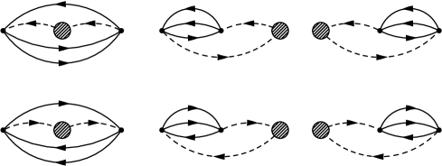
Figure 3: The six third-order two-particle reducible diagrams composed of one second-order and one first-order piece. Articulation lines are shown as dashed lines. The shaded blobs represent vertices with loops (first-order pieces). In each row, the diagram on the left is a normal diagram, and the other two are anomalous. The diagrams in each row transform into each other under cyclic vertex permutations. The set of all six diagrams is closed under general vertex permutations.

The normal third-order two-particle reducible diagrams are shown in Fig. 3. Also shown are the cyclically related anomalous diagrams. The cyclic expression for the sum of these diagrams is given by

$$\Omega_{3,(21)}^{\text{cyclic}} =-\frac{1}{4}\sum_{ijab}\zeta^{ijab}n_{ij}\bar{n}_{ab}\mathcal{F}_{(21)}^{\text{cyclic}}\big{(}n_{i}U_{1,i}-\bar{n}_{a}U_{1,a}\big{)},$$ (92)

where

$$\mathcal{F}_{(21)}^{\text{cyclic}}=\frac{1-\operatorname{\operatorname{e}}^{-\beta D}-\beta D\operatorname{\operatorname{e}}^{-\beta D}}{D^{2}},$$ (93)

with $D=D_{ab,ij}$. In Hartree-Fock MBPT, the contribution from these diagrams is (as is well known) canceled by the corresponding diagrams where the first-order pieces are replaced by $-U_{1}$ vertices. Nevertheless, it will be still be useful to regularize these contributions. We will then find that, if $U_{1}$ were left out, the anomalous part of these diagrams can still be canceled via $U_{2}^{\text{BdD}}$.

Substituting $D\rightarrow D+\text{i}\eta$ and applying Eqs. (14) and (19) and the relabeling $(i,j)\leftrightarrow(a,b)$, we can separate $\Omega_{3,(21)}^{\text{cyclic}}$ into the three contributions

$$\Omega_{3,(21),\text{normal}}^{\text{reduced,}\circ\circ,\div} =-\frac{1}{4}\sum_{ijab}\zeta^{ij,ab}n_{ij}\bar{n}_{ab}\frac{1}{(D+\text{i}\eta)^{2}}\big{(}U_{1,i}-U_{1,a}\big{)},$$ (94)

$$\Omega_{3,(21),\text{anom.}}^{\text{reduced,}\circ\circ,\div} =\frac{\beta}{4}\sum_{ijab}\zeta^{ij,ab}n_{ij}\bar{n}_{ab}\frac{1}{D+\text{i}\eta}\big{(}\bar{n}_{i}U_{1,i}-n_{a}U_{1,a}\big{)},$$ (95)

$$\Omega_{3,(21),\text{pseudo-a.}}^{\text{reduced,}\circ\circ,\div} =\frac{1}{4}\sum_{ijab}\zeta^{ij,ab}n_{ij}\bar{n}_{ab}\left[\frac{1}{(D+\text{i}\eta)^{2}}-\frac{1}{(D-\text{i}\eta)^{2}}\right]$$

$$\quad\times\big{(}n_{i}U_{1,i}-\bar{n}_{a}U_{1,a}\big{)}.$$ (96)

Here, ${\circ\circ}$ refers to an incomplete (in fact, incorrect) regularization: none of the three contributions given by Eq. (94), (95) and (III.1) is real, and (more severely) also their sum is not real. As explained below Eq. (III.1), the reason for this deficiency is that we have applied Eq. (19) and relabeled indices without applying the Sokhotski-Plemelj-Fox formula first. To repair this we have to average over the signs of the imaginary parts, which leads to

$$\Omega_{3,(21),\text{normal}}^{\text{reduced,}\ast\ast,\div} =-\frac{1}{8}\sum_{ijab}\zeta^{ij,ab}n_{ij}\bar{n}_{ab}$$

$$\quad\times\left[\frac{1}{(D+\text{i}\eta)^{2}}+\frac{1}{(D-\text{i}\eta)^{2}}\right]\big{(}U_{1,i}-U_{1,a}\big{)},$$ (97)

$$\Omega_{3,(21),\text{anom.}}^{\text{reduced,}\ast\ast,\div} =\frac{\beta}{8}\sum_{ijab}\zeta^{ij,ab}n_{ij}\bar{n}_{ab}\left[\frac{1}{(D+\text{i}\eta)}+\frac{1}{(D-\text{i}\eta)}\right],$$

$$\quad\times(\bar{n}_{i}U_{1,i}-n_{a}U_{1,a}),$$ (98)

$$\Omega_{3,(21),\text{pseudo-a.}}^{\text{reduced,}\ast\ast,\div} =0.$$ (99)

The pseudoanomalous contribution has vanished: this feature, which is essential to obtain the Fermi-liquid relations at $T\neq 0$ (but not ${T=0}$), holds to all orders (see Sec. IV). Note that the vanishing of the pseudoanomalous contributions holds only if all vertex permutations are included, i.e., it holds not separately for cyclically closed sets (in the present case, the two rows in Fig. 3).

The anomalous contribution has the factorized form given by Eq. (II.4.3) (with $\ast\ast$ instead of $\ast$), i.e.,

$$\Omega_{3,(21),\text{anom.}}^{\text{reduced,}\ast\ast,\div} =-\beta\,U_{2,i}^{\text{reduced,}\ast\ast,(\div)}n_{i}\bar{n}_{i}\,U_{1,i}.$$ (100)

Thus, the anomalous contribution from the diagrams of Fig. 3 gets canceled by the contribution from the diagram shown in Fig. 4 where one piece is a first-order diagram and the other one either a $-U_{1}$ vertex or a $-U_{2}^{\text{BdD}}$ vertex. The same cancellation occurs between the rotated diagram and the one with two mean-field vertices, and similar for the case where both $U_{1}$ and $U_{2}^{\text{BdD}}$ are included.

Figure 4: The anomalous diagram composed of two pieces of the mean-field or single-vertex loop type.

III.2 Integration variables

We now discuss how the formulas derived in Sec. III.1 can be evaluated in numerical calculations. Nonvanishing contributions with poles of even degree appear first at fourth order in the BdD renormalization scheme. These have to be evaluated in terms of the Hadamard finite part, which obviously represents a major difficulty in the numerical application of the BdD scheme at high orders. We leave out the discussion of methods to evaluate the Hadamard finite part numerically, and defer numerical applications of the BdD scheme (and the other schemes) to future research.

For an isotropic system and MBPT without a mean-field potential (${U_{\textbf{k}}=0}$) where $\varepsilon_{\textbf{k}}=\varepsilon_{0,\textbf{k}}=\textbf{k}^{2}/(2M)$, using as integration variables relative momenta $\textbf{p}=(\textbf{k}_{i}-\textbf{k}_{j})/2$ and $\textbf{A}=(\textbf{k}_{a}-\textbf{k}_{b})/2$ as well as the average momentum $\textbf{K}=(\textbf{k}_{i}+\textbf{k}_{j})/2=(\textbf{k}_{a}+\textbf{k}_{b})/2$, one obtains from Eq. (III.1) the following expression for the second-order normal contribution:

$$\Omega_{2,\text{normal}}^{\text{BdD}} =-2M\sum_{\textbf{K},\textbf{p},\textbf{A}}\zeta^{ijab}n_{ij}\bar{n}_{ab}\frac{P}{A^{2}-p^{2}}.$$ (101)

The functional derivative of this expression with respect to $n_{\textbf{k}_{i}}$ is given by

$$U_{2,\textbf{k}_{i}}^{\text{BdD}}[\varepsilon_{0,\textbf{k}_{i}}]=-4M\sum_{\textbf{p},\textbf{A}}\zeta^{ijab}\big{(}n_{j}\bar{n}_{ab}+n_{ab}\bar{n}_{j}\big{)}\frac{P}{A^{2}-p^{2}}.$$ (102)

For truncation order ${N=2}$, the single-particle energies in the BdD scheme are obtained from the self-consistent equation

$$\varepsilon_{\textbf{k}}=\frac{\textbf{k}^{2}}{2M}+U_{1,\textbf{k}}+U_{2,\textbf{k}}^{\text{BdD}}[\varepsilon_{\textbf{k}}],$$ (103)

where one may use for $U_{2,\textbf{k}}^{\text{BdD}}[\varepsilon_{\textbf{k}}]$ the expression obtained by substituting in Eq. (102) the term $D_{ab,ij}=\varepsilon_{\textbf{k}_{a}}+\varepsilon_{\textbf{k}_{b}}-\varepsilon_{\textbf{k}_{i}}-\varepsilon_{\textbf{k}_{j}}$ for $M/(A^{2}-p^{2})$ if this substitution does not introduce additional poles; otherwise one must go back to the expression with infinitesimal imaginary parts, Eq. (III.1). This issue can be seen also in the ${U_{\textbf{k}}=0}$ case if $\textbf{k}_{a}$, $\textbf{k}_{i}$ and $\textbf{k}_{j}$ are used as integration variables to evaluate Eq. (III.1). Considering a one-dimensional system for simplicity, we have

$$\Omega_{2,\text{normal}}^{\text{BdD}} =-\frac{M}{4}\!\!\sum_{k_{a},k_{i},k_{j}}\!\!\zeta^{ijab}n_{ij}\bar{n}_{ab}\,\left[\frac{1}{\kappa+\text{i}\eta}+\frac{1}{\kappa-\text{i}\eta}\right],$$ (104)

with $k_{b}=k_{i}+k_{j}-k_{a}$ and $\sum_{k}=\int dk/(2\pi)$. Moreover, $\kappa=(k_{a}-k_{i})(k_{a}-k_{j})$, i.e., now there are two poles. To bring Eq. (104) into a form where the Sokhotski-Plemelj theorem can be applied, we note that

$$(k_{a}-k_{i}+\text{i}\eta)(k_{a}-k_{j}+\text{i}\eta)$$

$$\quad\quad=(\kappa+\text{i}\eta)\,\theta(2k_{a}-k_{i}-k_{j})+(\kappa-\text{i}\eta)\,\theta(k_{i}+k_{j}-2k_{a}),$$ (105)

so

$$\sum_{\text{sgn}(\eta)}\frac{1}{\kappa+\text{i}\eta}=\sum_{\text{sgn}(\eta)}\frac{1}{(k_{a}-k_{i}+\text{i}\eta)(k_{a}-k_{j}+\text{i}\eta)}.$$ (106)

The Sokhotski-Plemelj theorem can now be applied (assuming that $k_{a}$ is integrated after $k_{i}$ or $k_{j}$), which leads to

$$\Omega_{2,\text{normal}}^{\text{BdD}} =-\frac{M}{2}\sum_{k_{a},k_{i},k_{j}}\zeta^{ijab}n_{ij}\bar{n}_{ab}$$

$$\quad\times\bigg{[}\frac{P}{k_{a}-k_{i}}\frac{P}{k_{a}-k_{j}}+\pi^{2}\delta(k_{a}-k_{i})\delta(k_{a}-k_{j})\bigg{]},$$ (107)

where the integration order is fixed. Changing the integration order such that $k_{a}$ is integrated first would lead to an incorrect result, as evident from the Poincaré-Bertrand transformation formula Hardy (1909); Poincaré (1910); Bertrand (1921); Muskhelishvili (2008); Davies et al. (1990)

$$\int\!\!dx\!\int\!\!dy\,\,\varphi(x,y)\frac{P}{x-y}\frac{P}{x-z}$$

$$\quad=\int\!\!dy\!\int\!\!dx\,\,\varphi(x,y)\frac{P}{x-y}\frac{P}{x-z}+\pi^{2}\varphi(z,z).$$ (108)

Since it has only one pole, the expression given by Eq. (101) is however preferable compared to the one where $\textbf{k}_{a}$, $\textbf{k}_{i}$ and $\textbf{k}_{j}$ are used as integration variables.

At third order the issue manifested by the Poincaré-Bertrand transformation formula becomes unavoidable. For an isotropic system and ${U_{\textbf{k}}=0}$, using relative and average momenta as integration variables one obtains for $\Omega_{3,\text{pp}}^{\text{BdD}}$ the expression (see also Refs. Kondo (1968); Yosida and Miwa (1969))

$$\Omega_{3,\text{pp}}^{\text{BdD}} =\frac{M^{2}}{3}\!\sum_{\textbf{K},\textbf{p},\textbf{A},\textbf{B}}\zeta^{ijabcd}_{\text{pp}}n_{ij}\bar{n}_{abcd}$$

$$\quad\times\left[3\frac{P}{A^{2}-p^{2}}\frac{P}{B^{2}-p^{2}}+\pi^{2}\frac{\delta(A-p)\delta(B-p)}{(A+p)(B+p)}\right],$$ (109)

where $\textbf{p}=(\textbf{k}_{i}-\textbf{k}_{j})/2$, $\textbf{A}=(\textbf{k}_{a}-\textbf{k}_{b})/2$, $\textbf{B}=(\textbf{k}_{c}-\textbf{k}_{d})/2$ and $\textbf{K}=(\textbf{k}_{i}+\textbf{k}_{j})/2$. In Eq. (III.2), the integration order is such that $p$ is integrated after $A$ or $B$. The expression for $\Omega_{3,\text{hh}}^{\text{BdD}}$ is similar to Eq. (III.2). For $\Omega_{3,\text{ph}}^{\text{BdD}}$, however, using relative and average momenta as integration variables leads to

$$\Omega_{3,\text{ph}}^{\text{BdD}} =\frac{8M^{2}}{3}\sum_{\textbf{K},\textbf{p},\textbf{A},\textbf{Y}}\zeta^{ijkabc}_{\text{ph}}n_{ijk}\bar{n}_{abc}$$

$$\quad\times\left[\mathcal{F}_{[\eta_{1},\eta_{2}]}+\mathcal{F}_{[-\eta_{1},\eta_{2}]}+\mathcal{F}_{[-\eta_{1},-\eta_{2}]}\right],$$ (110)

where $\textbf{p}=(\textbf{k}_{i}-\textbf{k}_{j})/2$, $\textbf{A}=(\textbf{k}_{a}-\textbf{k}_{b})/2$, $\textbf{Y}=(\textbf{k}_{a}-\textbf{k}_{c})/2$ and $\textbf{K}=(\textbf{k}_{i}+\textbf{k}_{j})/2$, and

$$\mathcal{F}_{[\eta_{1},\eta_{2}]}=\frac{1}{\big{[}A^{2}-p^{2}+\text{i}\eta_{1}\big{]}\,\big{[}(\textbf{p}-\textbf{A})\cdot(\textbf{A}-2\textbf{Y}+\textbf{p})+\text{i}\eta_{2}\big{]}}.$$ (111)

From here one would have to proceed similar to the steps that lead from Eq. (104) to Eq. (III.2).

IV Factorization to All Orders

Here, we prove to all orders that the BdD renormalization scheme implies the thermodynamic relations associated with Fermi-liquid theory and (consequently) leads to a perturbation series that manifests the concistency of the adiabatic zero-temperature formalism, for both isotropic and anisotropic systems.

First, in Sec. IV.1, we examine more closely how the linked-cluster theorem manifests itself. Second, in Sec. IV.2 we systematize the disentanglement ($\div$) of the grand-canonical perturbation series. These two steps provide the basis for Sec. IV.3, where we prove to all orders the reduced factorization property for finite systems, Eq. (II.4.3). In Sec. IV.4 we then infer that the reduced factorization property holds also for the BdD renormalization scheme. This implies the Fermi-liquid relations and the consistency of the adiabatic formalism. Finally, in Sec. IV.5 we point out that the BdD renormalization scheme maintains the cancellation of the divergencies (at ${T=0}$) from energy denominator poles and discuss the minimal renormalization requirement for the consistency of the adiabatic formalism with the modified perturbation series for the free energy, $F(T,\mu_{\text{ref}})$, in the anisotropic case.

IV.1 Linked-cluster theorem

Letting the truncation order (formally) go to infinity, the sum of all perturbative contributions to $\Omega(T,\mu)$ can be written as

$$\Delta\Omega=\sum_{n=1}^{\infty}\Omega_{n}=-\frac{1}{\beta}\ln\left[1-\beta\sum_{n=1}^{\infty}\Upsilon_{n}\right],$$ (112)

where $\Upsilon_{n}$ denotes the contribution of order $n$ from both linked and unlinked diagrams. We refer to the various linked parts of an unlinked diagram as subdiagrams. Further, we denote the contribution—evaluated via a given time-independent ($\aleph$) formula (i.e., direct, cyclic, or reduced with $\ast$ or $\ast\ast$)—to $\Upsilon_{n}$ from a diagram composed of $K=k\sum_{i=0}^{k}\alpha_{i}$ linked parts involving $k$ different subdiagram species $\Gamma_{1}\neq\Gamma_{2}\neq\ldots\neq\Gamma_{k}$ where each $\Gamma_{i}$ appears $\alpha_{i}$ times in the complete diagram, by $\Upsilon^{\aleph}_{[\Gamma_{1}^{\alpha_{1}}\cdots\Gamma_{k}^{\alpha_{k}}]_{n}}$. In this notation, Eq. (112) reads

$$\Delta\Omega=-\frac{1}{\beta}\ln\Big{[}1-\beta\sum_{n=1}^{\infty}\sum_{[\Gamma_{1}^{\alpha_{1}}\cdots\Gamma_{k}^{\alpha_{k}}]_{n}}\sum_{O}\Upsilon^{\aleph}_{[\Gamma_{1}^{\alpha_{1}}\cdots\Gamma_{k}^{\alpha_{k}}]_{n}}\Big{]},$$ (113)

where $\sum_{[\Gamma_{1}^{\alpha_{1}}\cdots\Gamma_{k}^{\alpha_{k}}]_{n}}$ is the sum over all possible (i.e., those consistent with order $n$) combinations of subdiagrams (including repetitions), and $\sum_{O}$ denotes the sum over all distinguishable vertex permutations of the unlinked diagram that leave the subdiagrams invariant. This is illustrated in Fig. 5. We write

$$\sum_{n=1}^{\infty}\sum_{[\Gamma_{1}^{\alpha_{1}}\cdots\Gamma_{k}^{\alpha_{k}}]_{n}}\sum_{O}\Upsilon^{\aleph}_{[\Gamma_{1}^{\alpha_{1}}\cdots\Gamma_{k}^{\alpha_{k}}]_{n}}=\sum_{\Gamma_{1}^{\alpha_{1}}\cdots\Gamma_{k}^{\alpha_{k}}}\sum_{O}\Upsilon^{\aleph}_{\Gamma_{1}^{\alpha_{1}}\cdots\Gamma_{k}^{\alpha_{k}}}.$$ (114)

It is

$$\sum_{\Gamma_{1}^{\alpha_{1}}\cdots\Gamma_{k}^{\alpha_{k}}}\sum_{O}\Upsilon^{\aleph}_{\Gamma_{1}^{\alpha_{1}}\cdots\Gamma_{k}^{\alpha_{k}}}=\sum_{\widetilde{\Gamma}_{1}^{\alpha_{1}}\cdots\widetilde{\Gamma}_{k}^{\alpha_{k}}}\sum_{P}\Upsilon^{\aleph}_{\widetilde{\Gamma}_{1}^{\alpha_{1}}\cdots\widetilde{\Gamma}_{k}^{\alpha_{k}}},$$ (115)

where $\sum_{P}$ denotes the sum over all distinguishable vertex orderings, and $\sum_{\widetilde{\Gamma}_{1}^{\alpha_{1}},\ldots,\widetilde{\Gamma}_{k}^{\alpha_{k}}}$ sums over all combinations of subdiagrams where in the underlying set of linked diagrams $\{\Gamma_{i}\}$ only one (arbitrary) element is included for each set of diagrams that is closed under vertex permutations. For example, among the first two diagrams of Fig. 2 only one is included, and only one of the six diagrams of Fig. 3.

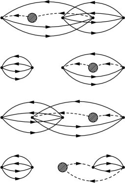
Figure 5: Vertex permutations for an unlinked diagram with two linked parts (subdiagrams). If the diagram in the first row represents the original vertex ordering, then the second and third diagram correspond to (nonoverlapping and overlapping, respectively) orderings $\in O$, and the fourth diagram to an ordering $\in P/O$.

The generalization of Eq. (8) for $\Upsilon_{n}$ is given by

$$\Upsilon_{n}^{\text{direct}[P]}=-\frac{1}{\beta}\frac{(-1)^{n}}{n!}\int\limits_{0}^{\beta}\!d\tau_{n}\cdots d\tau_{1}\;\Braket{\mathcal{T}\big{[}\mathcal{V}(\tau_{n})\cdots\mathcal{V}(\tau_{1})\big{]}}.$$ (116)

We denote the expressions obtained from Eq. (116) for the contribution from a given permutation invariant set of (linked or unlinked) diagrams by $\Upsilon^{\text{direct}[P]}_{\widetilde{\Gamma}_{1}^{\alpha_{1}}\cdots\widetilde{\Gamma}_{k}^{\alpha_{k}}}$. As noted in Sec. II.2, these expressions are equivalent to the summed expressions obtained from any of the time-independent formulas (direct, cyclic, or reduced with $\ast$ or $\ast\ast$), i.e.,

$$\Upsilon^{\text{direct}[P]}_{\widetilde{\Gamma}_{1}^{\alpha_{1}}\cdots\widetilde{\Gamma}_{k}^{\alpha_{k}}} =\sum_{P}\Upsilon^{\aleph}_{\widetilde{\Gamma}_{1}^{\alpha_{1}}\cdots\widetilde{\Gamma}_{k}^{\alpha_{k}}}.$$ (117)

Now, the number of ways the $n$ perturbation operators in Eq. (116) can be partitioned into the subgroups specified by $\Upsilon^{\text{direct}[P]}_{\widetilde{\Gamma}_{1}^{\alpha_{1}}\cdots\widetilde{\Gamma}_{k}^{\alpha_{k}}}$ is given by Abrikosov et al. (1975); Fetter and Walecka (1972)

$$\frac{1}{\alpha_{1}!\cdots\alpha_{k}!}\frac{n!}{(n_{1}!)^{\alpha_{1}}\cdots(n_{k}!)^{\alpha_{k}}},$$ (118)

where $n_{i}$ are the orders of the respective subdiagrams. From Eq. (116), this leads to

$$\sum_{P}\Upsilon^{\aleph}_{\widetilde{\Gamma}_{1}^{\alpha_{1}}\cdots\widetilde{\Gamma}_{k}^{\alpha_{k}}} =-\frac{1}{\beta}\prod_{i=1}^{k}\frac{\left(-\beta\,\Upsilon^{\text{direct}[P]}_{\widetilde{\Gamma}_{i}}\right)^{\alpha_{i}}}{\alpha_{i}!}$$

$$=-\frac{1}{\beta}\prod_{i=1}^{k}\frac{\left(-\beta\,\sum_{P_{i}}\Upsilon^{\aleph}_{\widetilde{\Gamma}_{i}}\right)^{\alpha_{i}}}{\alpha_{i}!},$$ (119)

where in the second step we have applied Eq. (117). In Sec. IV.3 we will see that Eq. (IV.1) implies the (direct, cyclic, and reduced) factorization properties for anomalous diagrams.

It is now straightforward to verify by explicit comparison with Eq. (IV.1) that

$$\sum_{\widetilde{\Gamma}_{1}^{\alpha_{1}}\cdots\widetilde{\Gamma}_{k}^{\alpha_{k}}}\sum_{P}\left(-\beta\Upsilon^{\aleph}_{\widetilde{\Gamma}_{1}^{\alpha_{1}}\cdots\widetilde{\Gamma}_{k}^{\alpha_{k}}}\right) =\sum_{\alpha=1}^{\infty}\frac{1}{\alpha!}\bigg{[}-\beta\sum_{\Gamma}\Upsilon^{\aleph}_{\Gamma}\bigg{]}^{\alpha}$$

$$=-1+\exp\Big{(}-\beta\sum_{\Gamma}\Upsilon^{\aleph}_{\Gamma}\Big{)}.$$ (120)

Applying this to Eq. (115) leads to

$$\Delta\Omega =\sum_{\Gamma}\Upsilon^{\aleph}_{\Gamma},$$ (121)

which constitutes the linked-cluster theorem. Now, expanding the logarithm in Eq. (112) we find

$$\Delta\Omega =\sum_{n=1}^{\infty}\,\Bigg{[}\sum_{\nu,\{n_{i}\},\{k_{i}\}}\beta^{k_{1}+\ldots+k_{\nu}-1}\binom{k_{1}+\ldots+k_{\nu}}{k_{1},\ldots,k_{\nu}}\frac{(\Upsilon_{n_{1}})^{k_{1}}\cdots(\Upsilon_{n_{\nu}})^{k_{\nu}}}{k_{1}+\ldots+k_{\nu}}\Bigg{]},$$ (122)

where the inner sum is subject to the constraints $\sum_{i=1}^{\nu}n_{i}k_{i}=n$, $1\leq n_{1}<n_{2}<\ldots<n_{\nu}$, $k_{i}\geq 1$, and $\nu\geq 1$. The linked-cluster theorem implies that, if evaluated in terms of the usual Wick contraction formalism Fetter and Walecka (1972), in Eq. (122) the contributions with $\nu=1$ and $k_{1}=1$ from unlinked diagrams are all canceled by the contributions with $\nu>1$ or $k_{1}>1$. The individual expressions from these canceling terms are not size extensive, i.e., in the thermodynamic limit they diverge with higher powers of the confining volume.

IV.2 Disentanglement

Here, we first introduce the cumulant formalism, which allows systematizing the disentanglement ($\div$). Then, we show that this formalism provides a new representation and evaluation method for the contributions associated (in the usual Wick contraction formalism) with anomalous diagrams and the subleading parts of Eqs. (15)–(18), etc. Finally, we construct and discuss the modified perturbation series for the free energy $F(T,\mu_{\text{ref}})$.

IV.2.1 Cumulant formalism

We define $\mathcal{C}_{i_{1}\ldots i_{n}}$ as the unperturbed ensemble average of a fully-contracted (indicted by paired indices) but not necessarily linked sequence of creation and annihilation operators, i.e.,

$$\mathcal{C}_{i_{1}\ldots i_{n}}=\braket{a_{i_{1}}^{\dagger}a_{i_{1}}\cdots a_{i_{n}}^{\dagger}a_{i_{n}}},$$ (123)

where some of the index tuples may be identical (articulation lines). In Eq. (123), all contractions are of the hole type. For the case where there are also particles we introduce the notation

$$\mathcal{C}_{i_{1}\cdots i_{n}}^{a_{1}\cdots a_{m}}=\braket{a_{i_{1}}^{\dagger}a_{i_{1}}\cdots a_{i_{n}}^{\dagger}a_{i_{n}}a_{a_{1}}a_{a_{1}}^{\dagger}\cdots a_{a_{m}}b_{a_{m}}^{\dagger}}.$$ (124)

This can be expressed in terms of functional derivatives of the unperturbed partition function $\mathcal{Y}_{\!\text{ref}}=\operatorname{\operatorname{Tr}}[\operatorname{\operatorname{e}}^{-\beta(\mathcal{H}_{\text{ref}}-\mu\mathcal{N})}]$, i.e.,

$$\mathcal{C}_{i_{1}\cdots i_{n}}^{a_{1}\cdots a_{m}} =\frac{1}{\mathcal{Y}_{\!\text{ref}}}\frac{\delta}{\delta[-\beta\varepsilon_{i_{1}}]}\cdots\frac{\delta}{\delta[-\beta\varepsilon_{i_{n}}]}$$

$$\quad\times\bigg{(}1-\frac{\delta}{\delta[-\beta\varepsilon_{a_{1}}]}\bigg{)}\cdots\bigg{(}1-\frac{\delta}{\delta[-\beta\varepsilon_{a_{m}}]}\bigg{)}\;\mathcal{Y}_{\!\text{ref}}.$$ (125)

This shows that the upper indices can be lowered iteratively, i.e., $\mathcal{C}_{i_{1}\cdots i_{n}}^{a_{1}\cdots a_{m}}=\mathcal{C}_{i_{1}\cdots i_{n}}^{a_{1}\cdots a_{m-1}}-\mathcal{C}_{i_{1}\cdots i_{n}a_{m}}^{a_{1}\cdots a_{m-1}}$, which leads to

$$\mathcal{C}_{i_{1}\cdots i_{n}}^{a_{1}\cdots a_{m}}=\sum_{\mathcal{P}\subset\{1,\ldots,m\}}(-1)^{|P|}\mathcal{C}_{i_{1}\cdots i_{n}\{a_{k}\}_{k\in P}}.$$ (126)

The cumulants $\mathcal{K}_{i_{1}\ldots i_{n}}$ are defined by

$$\mathcal{K}_{i_{1}\ldots i_{n}}=\frac{\delta^{n}\ln\mathcal{Y}_{\!\text{ref}}}{\delta[-\beta\varepsilon_{i_{1}}]\cdots\delta[-\beta\varepsilon_{i_{n}}]}.$$ (127)

The relation between the $\mathcal{K}$’s and the $\mathcal{C}$’s is given by Fernández et al. (1991)

$$\mathcal{C}_{i_{1}\cdots i_{n}}=\sum_{\begin{subarray}{c}\mathcal{P}\in\,\text{partitions}\\ \text{of}\,\{1,\ldots,n\}\end{subarray}}\prod_{I\in\mathcal{P}}\mathcal{K}_{\{i_{k}\}_{k\in I}}.$$ (128)

These formulas provide an alternative way (compared to the Wick contraction formalism) to evaluate the various contributions $\Upsilon_{[\Gamma_{1}^{\alpha_{1}}\cdots\Gamma_{k}^{\alpha_{k}}]_{n}}$ in Eq. (122).

IV.2.2 Simply connected unlinked diagrams

For linked diagrams without articulation lines (i.e., two-particle irreducible diagrams) the contributions from higher cumulants have measure zero for infinite systems. For such diagrams, the (sums of the) contributions from higher cumulants vanish also in the finite case, via exchange antisymmetry. This is clear, since these (nonextensive) contributions are absent in the Wick contraction formalism. For instance, for the first-order diagram $\mathcal{C}_{ij}=\mathcal{K}_{i}\mathcal{K}_{j}+\delta_{ij}\mathcal{K}_{ii}$ the part $\delta_{ij}\mathcal{K}_{ii}$ gives no contribution (by antisymmetry). Overall, it is

$$i_{1}\neq i_{2}\neq\ldots\neq i_{n}:\;\;\;\mathcal{C}_{i_{1}\cdots i_{n}}=\prod_{\nu=1}^{n}\mathcal{K}_{i_{\nu}}$$ (129)

for linked diagrams. This means that for linked two-particle irreducible diagrams the cumulant formalism leads to the same expressions as the Wick contraction formalism. For two-particle reducible diagrams, however, there are additional size extensive contributions from higher cumulants corresponding to articulation lines with identical three-momenta. This has the effect that for each set of normal articulation lines with identical three-momenta there is only a single distribution function, i.e.,

$$\mathcal{C}_{i_{1}\cdots i_{n}j\cdots j}^{a_{1}\cdots a_{m}} =\mathcal{C}_{i_{1}\cdots i_{n}j}^{a_{1}\cdots a_{m}},$$ (130)

$$\mathcal{C}_{i_{1}\cdots i_{n}}^{a_{1}\cdots a_{m}b\cdots b} =\mathcal{C}_{i_{1}\cdots i_{n}}^{a_{1}\cdots a_{m}b},$$ (131)

see Ref. Wellenhofer (2017). For example, $\mathcal{C}_{i_{1}\ldots i_{n}jj}=\mathcal{C}_{i_{1}\ldots i_{n}}(\mathcal{K}_{j}\mathcal{K}_{j}+\mathcal{K}_{jj})=\mathcal{C}_{i_{1}\ldots i_{n}j}$, since $\mathcal{K}_{j}\mathcal{K}_{j}+\mathcal{K}_{jj}=n_{j}n_{j}+n_{j}\bar{n}_{j}=n_{j}$. Equations (130) and (131) together with Eq. (126) imply that the contributions from anomalous diagrams are zero:

$$\mathcal{C}_{i_{1}\cdots i_{n}j\cdots j}^{a_{1}\cdots a_{m}j\cdots j}=0.$$ (132)

The contributions from anomalous diagrams and from the subleading parts of Eqs. (15)–(18), etc. , now arise instead from unlinked diagrams (with normal subdiagrams). That is, for unlinked diagrams composed of $N$ subdiagrams the contributions from higher cumulants connecting $N$ lines with distinct three-momenta are size extensive. For example, for the case of three first-order subdiagrams with indices $(i,j)$, $(k,l)$, and $(m,n)$ one has the contributions

$$\delta_{ik}\delta_{jm}\mathcal{K}_{ii}\mathcal{K}_{jj}\mathcal{K}_{l}\mathcal{K}_{n},\ldots,\;\;\delta_{ik}\delta_{im}\mathcal{K}_{iii}\mathcal{K}_{j}\mathcal{K}_{l}\mathcal{K}_{n},\ldots,$$ (133)

where $\mathcal{K}_{iii}=n_{i}\bar{n}_{i}\bar{n}_{i}-n_{i}n_{i}\bar{n}_{i}$ and the ellipses represent terms with other index combinations. By virtue of the linked-cluster theorem, the size extensive contributions from unlinked diagrams where not all higher-cumulant indices correspond to different subdiagrams cancel against the corresponding terms with $\nu>1$ or $k_{1}>1$ in Eq. (122). The remaining size extensive contributions from unlinked diagrams are exactly those where the different (normal) subdiagrams are simply connected via higher cumulants. This provides a new representation for the contributions associated (in the Wick contraction formalism) with anomalous diagrams and the contributions not included in Eqs. (130) and (131).

IV.2.3 Modified thermodynamic perturbation series

There are two methods for the construction of the modified perturbation series for the free energy $F(T,\mu_{\text{ref}})$. The first, introduced by Kohn and Luttinger Kohn and Luttinger (1960), is based on grand-canonical MBPT; it constructs $F(T,\mu_{\text{ref}})$ in terms of a truncated formal expansion of $F(T,\mu)$ about $\mu_{\text{ref}}$, see Refs. Kohn and Luttinger (1960); Wellenhofer et al. (2014); Wellenhofer (2017) for details. The second method, due to Brout and Englert Brout and Englert (1960), starts from the canonical ensemble. In canonical perturbation theory Glassgold et al. (1959); Parry (1973), Eq. (123) is replaced by

$$\mathscr{C}_{i_{1}\ldots i_{n}}=\braket{a_{i_{1}}^{\dagger}a_{i_{1}}\cdots a_{i_{n}}^{\dagger}a_{i_{n}}}_{\!\varrho},$$ (134)

where $\braket{\ldots}_{\!\varrho}$ denotes the unperturbed canonical ensemble average which involves only Fock states $\ket{\Psi_{\!\varrho}}$ with fixed $\varrho=\Braket{\Psi_{\!\varrho}}{\mathcal{N}}{\Psi_{\!\varrho}}$. From this, we proceed analogously to the grand-canonical case, with $\mathcal{Y}_{\!\text{ref}}$ replaced by the unperturbed canonical partition function $\mathcal{Z}_{\text{ref}}=\sum_{\Psi_{\!\varrho}}\braket{\Psi_{\!\varrho}}{\operatorname{\operatorname{e}}^{-\beta\mathcal{H}_{\text{ref}}}}{\Psi_{\!\varrho}}$, i.e., the cumulants are now given by

$$\mathscr{K}_{i_{1}\ldots i_{n}}=\frac{\delta^{n}\ln\mathcal{Z}_{\text{ref}}}{\delta[-\beta\varepsilon_{i_{1}}]\cdots\delta[-\beta\varepsilon_{i_{n}}]}.$$ (135)

The decisive new step is now to evaluate the cumulants not directly (which would be practically impossible) but using the Legendre transformation

$$\ln\mathcal{Z}_{\text{ref}}(T,\varrho) =\ln\mathcal{Y}_{\!\text{ref}}(T,\mu_{\text{ref}})-\mu_{\text{ref}}\frac{\partial\ln\mathcal{Y}_{\!\text{ref}}(T,\mu_{\text{ref}})}{\partial\mu_{\text{ref}}},$$ (136)

where $\mu_{\text{ref}}$ is the chemical potential of an unperturbed grand-canonical system with the same mean fermion number as the fully interacting canonical system, i.e.,

$$\varrho=-\frac{1}{\beta}\frac{\partial\ln\mathcal{Y}_{\!\text{ref}}(T,\mu_{\text{ref}})}{\partial\mu_{\text{ref}}}=-\frac{\partial\Omega_{\text{ref}}(T,\mu_{\text{ref}})}{\partial\mu_{\text{ref}}}=\sum_{\textbf{k}}\tilde{n}_{\textbf{k}},$$ (137)

where $\tilde{n}_{\textbf{k}}$ denotes the Fermi-Dirac distribution with $\mu_{\text{ref}}$ as the chemical potential. With $\varrho$ being fixed, $\varrho=\sum_{\textbf{k}}\tilde{n}_{\textbf{k}}$ determines $\mu_{\text{ref}}$ as a functional of the spectrum $\varepsilon_{\textbf{k}}$. From this and Eq. (136), the expression for $\mathscr{K}_{i}$ is given by

$$\mathscr{K}_{i} =\frac{\delta\ln\mathcal{Y}_{\!\text{ref}}}{\delta[-\beta\varepsilon_{i}]}-\frac{1}{\beta}\frac{\partial\ln\mathcal{Y}_{\!\text{ref}}}{\partial\mu_{\text{ref}}}\Bigg{(}\frac{\delta\mu_{\text{ref}}}{\delta\varepsilon_{i}}\Bigg{)}_{\!\varrho}-\varrho\,\Bigg{(}\frac{\delta\mu_{\text{ref}}}{\partial\varepsilon_{i}}\Bigg{)}_{\!\varrho}=\tilde{n}_{i}.$$ (138)

The higher $\mathscr{K}$’s can then be determined iteratively, i.e.,

$$\mathscr{K}_{i_{1}i_{2}} =\Bigg{(}\frac{\delta\mathscr{K}_{i_{1}}}{\delta[-\beta\varepsilon_{i_{2}}]}\Bigg{)}_{\!\varrho}$$

$$=\delta_{i_{1}i_{2}}\frac{\partial\mathscr{K}_{i_{1}}}{\partial[-\beta\varepsilon_{i_{1}}]}-\frac{\partial\mathscr{K}_{i_{1}}}{\partial\mu_{\text{ref}}}\,\Bigg{[}\frac{\partial\varrho}{\partial\mu_{\text{ref}}}\Bigg{]}^{-1}\!\!\frac{\delta\varrho}{\delta[-\beta\varepsilon_{i_{2}}]}$$

$$=\delta_{i_{1}i_{2}}\tilde{n}_{i_{1}}(1-\tilde{n}_{i_{1}})-\frac{\tilde{n}_{i_{1}}(1-\tilde{n}_{i_{1}})\tilde{n}_{i_{2}}(1-\tilde{n}_{i_{2}})}{\sum_{i}\tilde{n}_{i}(1-\tilde{n}_{i})}.$$ (139)

For $\mathscr{K}_{i_{1}i_{2}i_{3}}$ and beyond there is also a contribution where the energy derivative acts on $[\partial\varrho/\partial\mu_{\text{ref}}]^{-1}=\sum_{i}\tilde{n}_{i}(1-\tilde{n}_{i})$, i.e.,

$$\big{[}\mathscr{K}_{i_{1}i_{2}i_{3}}\big{]}_{i_{1}\neq i_{2}\neq i_{3}} =-\frac{\partial\mathscr{K}_{i_{1}i_{2}}}{\partial\mu_{\text{ref}}}\Bigg{[}\frac{\delta\varrho}{\delta\mu_{\text{ref}}}\Bigg{]}^{-1}\frac{\delta\varrho}{\delta[-\beta\varepsilon_{i_{3}}]}$$

$$\quad-\frac{\partial\mathscr{K}_{i_{1}}}{\beta\mu_{\text{ref}}}\frac{\delta\varrho}{\delta[-\beta\varepsilon_{i_{2}}]}\frac{\partial}{\partial[-\beta\varepsilon_{i_{3}}]}\Bigg{[}\frac{\partial\varrho}{\partial\mu_{\text{ref}}}\Bigg{]}^{-1}.$$ (140)

One can show that $\big{[}\mathscr{K}_{i_{1}\ldots i_{n}}\big{]}_{i_{a}\neq i_{b}\,\forall a,b\in[1,n]}=\mathcal{O}(1/\varrho^{n-1})$, see Ref. Wellenhofer (2017), so the size extensive contributions from unlinked diagrams are again given by simply connected diagrams. For isotropic systems the anomalous parts of these contributions cancel at each order in the zero-temperature limit, thus

$$\text{isotropy:}\;\;F(T,\mu_{\text{ref}})\xrightarrow{T\rightarrow 0}E^{(0)}(\varepsilon_{\text{F}}),$$ (141)

with $\mu_{\text{ref}}\xrightarrow{T\rightarrow 0}\varepsilon_{\text{F}}$. By construction, within each of the order-by-order renormalization schemes (direct, cyclic, BdD), at each order the modified perturbation series $F(T,\mu_{\text{ref}})$ matches the grand-canonical perturbation series for the free energy $F(T,\mu)=\Omega(T,\mu)-\mu\,\partial\Omega(T,\mu)/\partial\mu$. The zero-temperature limit exists however only for the BdD scheme (see Sec. II).

IV.3 Factorization theorem(s)

Using the direct formula, the cyclic formula, or the reduced formula for finite systems ($\ast$) and applying the cumulant formalism to Eq. (IV.1) leads to

$$\sum_{P/A}\Upsilon^{\text{direct},\div}_{[\widetilde{\Pi}_{1}^{\alpha_{1}}\cdots\widetilde{\Pi}_{k}^{\alpha_{k}}]_{n}} =-\frac{1}{\beta}\prod_{i=1}^{k}\frac{\left(-\beta\,\sum_{P_{i}/A_{i}}\Upsilon^{\text{direct},\div}_{\widetilde{\Pi}_{i}}\right)^{\alpha_{i}}}{\alpha_{i}!},$$ (142)

$$\sum_{P/A}\Upsilon^{\text{cyclic},\div}_{[\widetilde{\Pi}_{1}^{\alpha_{1}}\cdots\widetilde{\Pi}_{k}^{\alpha_{k}}]_{n}} =-\frac{1}{\beta}\prod_{i=1}^{k}\frac{\left(-\beta\,\sum_{P_{i}/A_{i}}\Upsilon^{\text{cyclic},\div}_{\widetilde{\Pi}_{i}}\right)^{\alpha_{i}}}{\alpha_{i}!},$$ (143)

$$\sum_{P/A}\Upsilon^{\text{reduced,}\ast,(\div)}_{[\widetilde{\Pi}_{1}^{\alpha_{1}}\cdots\widetilde{\Pi}_{k}^{\alpha_{k}}]_{n}} =-\frac{1}{\beta}\prod_{i=1}^{k}\frac{\left(-\beta\,\sum_{P_{i}/A_{i}}\Upsilon^{\text{reduced,}\ast,\div}_{\widetilde{\Pi}_{i}}\right)^{\alpha_{i}}}{\alpha_{i}!},$$ (144)

where the $\widetilde{\Pi}_{i}$ are all normal diagrams, and $P/A$ excludes those permutations that lead to anomalous diagrams. The combinatorics (and sign factors) of the higher-cumulant connections matches the combinatorics of the functional derivatives that generate the mean-field contributions from the perturbative contributions to the grand-canonical potential. Hence, Eqs. (142) and (143) prove the direct and the cyclic version of the factorization property given by Eq. (35) and its cyclic analog, and Eq. (144) proves the reduced factorization property for finite systems $(\ast)$, Eq. (II.4.3). Note that Eq. (144) implies that in the reduced finite case the pseudoanomalous contributions vanish at each order.

The reduced version of the factorization theorem can also be proved as follows. For a given unlinked diagram where none of the linked parts are overlapping (see Fig. 5), the reduced formula has the form

$$\Upsilon^{\text{reduced,}\ast,(\div)}_{[{\Pi}_{1}^{\alpha_{1}}\cdots{\Pi}_{k}^{\alpha_{k}}]_{n}} \sim\underset{z=0}{\text{Res}}\frac{\operatorname{\operatorname{e}}^{-\beta z}}{z}\frac{1}{(-z)^{K}}\prod_{i}\frac{1}{D_{i}-z}$$

$$\sim\beta^{K-1}\prod_{i}\frac{1}{D_{i}}+\text{extra terms},$$ (145)

where the extra terms are proportional to $\beta^{K-n}$, with $n\in\{2,\ldots,K\}$. The reduced expressions for unlinked diagrams with overlapping linked parts are composed entirely of such extra terms. These extra terms are incompatible with the linked-cluster theorem: they do not match the temperature dependence of (the disentangled reduced expressions) for the corresponding contributions with $\nu>1$ or $k_{1}>1$ in Eq. (122). The extra terms must therefore cancel each other at each order in the sum $\sum_{P/A}$. Thus, symbolically we have

$$\sum_{P/A}\Upsilon^{\text{reduced,}\ast,(\div)}_{[\widetilde{\Pi}_{1}^{\alpha_{1}}\cdots\widetilde{\Pi}_{k}^{\alpha_{k}}]_{n}} \sim\beta^{K-1}\sum_{P/A}\left[\prod_{i}\frac{1}{D_{i}}\right],$$ (146)

which is equivalent to Eq. (144).

IV.4 Statistical quasiparticles

The energy denominator regularization maintains the linked-cluster theorem. From the proof of the (reduced) factorization theorem it can be inferred that this suffices to establish that

$$\sum_{P/A}\Upsilon^{\text{reduced,}\ast\ast,\div}_{[\widetilde{\Pi}_{1}^{\alpha_{1}}\cdots\widetilde{\Pi}_{k}^{\alpha_{k}}]_{n}} =-\frac{1}{\beta}\prod_{i=1}^{k}\frac{\left(-\beta\,\sum_{P_{i}/A_{i}}\Upsilon^{\text{reduced,}\ast\ast,\div}_{\widetilde{\Pi}_{i}}\right)^{\alpha_{i}}}{\alpha_{i}!},$$ (147)

which (by virtue of the cumulant formalism) implies the BdD factorization property

$$\Omega_{n_{1}+n_{2},\text{anomalous}}^{\text{reduced,}\ast\ast,\div} =-\frac{\beta}{2}\sum_{\textbf{k}}U^{\text{reduced,}\ast\ast,\div}_{n_{1},\textbf{k}}n_{\textbf{k}}\bar{n}_{\textbf{k}}\,U^{\text{reduced,}\ast\ast,\div}_{n_{2},\textbf{k}}$$

$$\quad\times(2-\delta_{n_{1},n_{2}}),$$ (148)

and similar [i.e., as specified by Eq. (147)] for anomalous contributions with several pieces (subdiagrams, in the cumulant formalism).

It is now clear how the cancellation between the contributions from simply connected diagrams composed of $V$ vertices and those where also $-U$ vertices are present works. For a given simply connected diagram, only the subdiagrams with single higher-cumulant connections can be replaced by $-U$ vertices, so at truncation orders $2N+1$ and $2N+2$ all anomalous contributions are removed if the mean field includes all contributions $U^{\aleph,\div}_{n,\textbf{k}}$ with $n\leq N$. However, this does not imply consistency with the adiabatic formalism for $U^{\aleph,\div}_{n,\textbf{k}}=U^{\text{reduced},\ast\ast,\div}_{n,\textbf{k}}$ (irrespective of isotropy), since the relation between chemical potential $\mu$ and the fermion number $\varrho$ does not match the adiabatic relation $\varrho=\sum_{\textbf{k}}\theta(\varepsilon_{\text{F}}-\varepsilon_{\textbf{k}})$. For the consistency of the grand-canonical and the adiabatic formalism, the BdD mean field must include all contributions up to the truncation order; only then one preserves the thermodynamic relations of the pure mean-field theory (where ${H=H_{0}+U}$, with $U\equiv U[n_{\textbf{k}}]$), i.e., the Fermi-liquid relations

$$\varrho =\sum_{\textbf{k}}n_{\textbf{k}},$$ (149)

$$S =-\sum_{\textbf{k}}\big{(}n_{\textbf{k}}\ln n_{\textbf{k}}+\bar{n}_{\textbf{k}}\ln\bar{n}_{\textbf{k}}\big{)},$$ (150)

$$\frac{\delta E}{\delta n_{\textbf{k}}} =\varepsilon_{\textbf{k}}.$$ (151)

These relations are valid for all temperatures.

IV.5 Zero-temperature limit

At zero temperature, the energy denominator poles are at the boundary of the integration region, which implies that the contributions from two-particle reducible diagrams with several identical energy denominators diverge Wellenhofer et al. (2018); Feldman et al. (1996). For MBPT with ${U=0}$ or ${U=U_{1}}$ one finds that the divergent contributions cancel each other at each order. This cancellation is maintained in the BdD renormalization scheme: the cancellation occurs separately for normal contributions, and for the sum of the matching contributions the Sokhotski-Plemelj-Fox formula is consistent with the ${T\rightarrow 0}$ limit.

Notably, the energy denominator regularization is not required to construct a thermodynamic perturbation series that is consistent with the adiabatic formalism in the anisotropic case: at ${T=0}$, the BdD factorization theorem takes the form

$$T=0:\;\;\Omega_{n_{1}+n_{2},\text{anomalous}} =-\frac{1}{2}\sum_{\textbf{k}}U^{\text{reduced},\ast\ast,\div}_{n_{1},\textbf{k}}\delta(\varepsilon_{\textbf{k}}-\mu)$$

$$\quad\times U^{\text{reduced},\ast\ast,\div}_{n_{2},\textbf{k}}(2-\delta_{n,m}),$$ (152)

and similar for anomalous diagrams with several pieces. (At ${T=0}$, the symbols $\ast\ast$ and $\div$ (and the specification of $\aleph$ to reduced) are not needed for the separation of normal and anomalous contributions to the grand-canonical potential.) Thus, as recognized by Feldman et al. Feldman et al. (1999), to cancel the anomalous contributions to $\Omega(T=0,\mu)$ the following mean field is sufficient (for truncation orders below $2N+2$):

$$U^{L_{\text{F}}}_{\textbf{k}}=U_{1,\textbf{k}}+\sum_{n=2}^{N}L_{\text{F}}\left[U^{\text{reduced,}\ast\ast,\div}_{n,\textbf{k}}(T=0,\mu)\right],$$ (153)

where $L_{\text{F}}$ satisfies $L_{\text{F}}[g(\textbf{k})]=g(\textbf{k})$ for $\varepsilon_{\textbf{k}}=\mu$ and is smoothed off away from $\varepsilon_{\textbf{k}}=\mu$. There are still anomalous contributions to the particle number, so the adiabatic series is not reproduced. The renormalization given by Eq. (153) (with $\mu$ replaced by $\mu_{\text{ref}}$) is however sufficient for the consistency of the adiabatic formalism with the modified perturbation series $F(T,\mu_{\text{ref}})$ in the anisotropic case.

V Conclusion

In the present paper, we have, substantiating the outline by Balian and de Dominicis (BdD) Balian and de Dominicis (1960); de Dominicis (1960), derived a thermodynamic perturbation series for infinite Fermi systems that (1) is consistent with the adiabatic zero-temperature formalism for both isotropic and anisotropic systems and (2) satisfies at each order and for all temperatures the thermodynamic relations associated with Fermi-liquid theory. This result arises, essentially, as a corollary of the linked-cluster theorem. The proof of (2) [which implies (1)] given here relies, apart from the earlier analysis of the disentanglement ($\div$) conducted by Balian, Bloch, and de Dominicis Balian et al. (1961a) and the outline provided by Balian and de Dominicis, on the application of the cumulant formalism (as a systematic method to perform $\div$) introduced by Brout and Englert Brout and Englert (1960); Brout (1959). The statistical quasiparticles associated with the thermodynamic Fermi-liquid relations are distinguished from the dynamical quasiparticles associated with the asymptotic stability of the low-lying excited states; in particular, the energies of dynamical and statistical quasiparticles are different.

In the perturbation series derived in the present paper thereference Hamiltonian is renormalized at each order in terms of additional contributions to the self-consistent mean-field potential. Conceptually, such an order-by-order renormalization is appealing: At each new order, not only is new information about interaction effects included, but this information automatically improves the reference point. Nevertheless, the relevance of this perturbation series depends on its convergence rate compared to the modified perturbation series for the free energy $F(T,\mu_{\text{ref}})$ with a fixed reference Hamiltonian; e.g., Hartree-Fock, or the (modified) second-order BdD mean field. In addition to the complete removal of anomalous contributions, the higher-order mean-field contributions lead also to partial cancellations of normal two-particle reducible contributions. This suggests that the convergence rate may indeed improve by renormalizing the mean field at each order. Apart from the question of convergence, beyond second order the practicality of the BdD renormalization scheme is impeded by the increasingly complicated regularization procedure required for its numerical application.

An alternative renormalization scheme, the direct scheme, was introduced by Balian, Bloch, and de Dominicis Balian et al. (1961a) (and rederived in the present paper, together with yet another scheme, the cyclic one). The thermodynamic relations resulting from the direct scheme however deviate from the Fermi-liquid relations. More severely, for the direct (and the cyclic) scheme the zero-temperature limit does not exist. The direct scheme may however still be useful for numerical calculations close to the classical limit. In particular, the corresponding perturbation series reproduces the virial expansion in the classical limit Balian et al. (1961b). The BdD renormalization scheme is thus mainly targeted at calculations not too far from the degenerate limit, in particular perturbative nuclear matter calculations (see, e.g., Refs. Bogner et al. (2005); Hebeler and Schwenk (2010); Hebeler et al. (2011); Tews et al. (2013); Krüger et al. (2013); Drischler et al. (2014, 2016a, 2016b, 2019); Coraggio et al. (2013, 2014); Sammarruca et al. (2015, 2018). Notably, the statistical quasiparticle relations may be useful for the application of the Sommerfeld expansion Constantinou et al. (2015) and to connect with phenomenological parametrizations Yasin et al. (2018).

In conclusion, future research in the many-fermion problem will investigate the perturbation series derived in the present paper.

I thank A. Carbone, C. Drischler, K. Hebeler, J. W. Holt, F. Hummel, N. Kaiser, R. Lang, M. Prakash, S. Reddy, A. Schwenk and W. Weise for useful discussions. Moreover, I thank the referees for helpful comments. Finally, I thank for their warm hospitality the group T39 (TU München), the INT (Seattle), the CEA (Saclay) and the ECT* (Trento), where parts of this work have been presented. This work is supported by the Deutsche Forschungsgemeinschaft (DFG, German Research Foundation) – Projektnummer 279384907– SFB 1245 as well as the DFG and NSFC through the CRC 110 “Symmetries and the Emergence of Structure in QCD”.

Appendix A Two-particle reducible diagrams at fourth order

Here we derive explicitly the regularized ($\ast\ast$) disentangled ($\div$) reduced expressions for the contributions from two-particle reducible diagrams at fourth order. Diagrams with single-vertex loops are canceled by the ones with $-U_{1}$ vertices; the remaining diagrams with $V$ vertices only are shown in Fig. 6. One can choose indices such that for each diagram the matrix elements are given by

$$\zeta=V^{ij,ab}V^{ik,cd}V^{cd,ki}V^{ab,ij},$$ (154)

and the energy denominators corresponding to the two second-order pieces are given by $D_{1}=D_{ab,ij}$ and $D_{2}=D_{cd,ik}$. The cyclic expression for the sum of the diagrams in each row $\nu\in\{1,2,3,4\}$ can then be written as

$$\Omega^{\text{cyclic}}_{4,\nu}=\xi_{\nu}\sum_{ijkabcd}\zeta\;\mathcal{N}_{\nu}\,\mathcal{F}_{\nu}^{\text{cyclic}},$$ (155)

where $\xi_{1,2,3,4}=(-1/4,-1/4,1/8,1/8)$. For the chosen indices the $\mathcal{N}_{\nu}$ are fixed as $\mathcal{N}_{1}=\mathcal{N}_{2}=n_{iijk}\bar{n}_{abcd}$,$\mathcal{N}_{3}=n_{iijcd}\bar{n}_{abk}$, and $\mathcal{N}_{4}=n_{abk}\bar{n}_{iijcd}$. Finally, from Eq. (10), the $\mathcal{F}^{\text{cyclic}}_{\nu}$ are given by

$$\mathcal{F}_{1}^{\text{cyclic}} =\frac{1}{D_{1}^{2}D_{1+2}}-\frac{\operatorname{\operatorname{e}}^{-\beta(D_{1+2})}}{D_{2}^{2}D_{1+2}}+\frac{\operatorname{\operatorname{e}}^{-\beta D_{1}}D_{1-2}}{D_{1}^{2}D_{2}^{2}}-\beta\frac{\operatorname{\operatorname{e}}^{-\beta D_{1}}}{D_{1}D_{2}},$$ (156)

$$\mathcal{F}_{2}^{\text{cyclic}} =\frac{1}{D_{1}D_{2}D_{1+2}}-\frac{\operatorname{\operatorname{e}}^{-\beta(D_{1+2})}}{D_{1}D_{2}D_{1+2}}+\frac{\operatorname{\operatorname{e}}^{-\beta D_{1}}}{D_{1}D_{2}D_{1-2}}$$

$$\quad-\frac{\operatorname{\operatorname{e}}^{-\beta D_{2}}}{D_{1}D_{2}D_{1-2}},$$ (157)

$$\mathcal{F}_{3}^{\text{cyclic}} =\frac{1}{D_{1}^{2}D_{1-2}}-\frac{\operatorname{\operatorname{e}}^{-\beta(D_{1-2})}}{D_{2}^{2}D_{1-2}}+\frac{\operatorname{\operatorname{e}}^{-\beta D_{1}}D_{1+2}}{D_{1}^{2}D_{2}^{2}}+\beta\frac{\operatorname{\operatorname{e}}^{-\beta D_{1}}}{D_{1}D_{2}},$$ (158)

$$\mathcal{F}_{4}^{\text{cyclic}} =-\frac{1}{D_{1}^{2}D_{1-2}}+\frac{\operatorname{\operatorname{e}}^{\beta(D_{1-2})}}{D_{2}^{2}D_{1-2}}-\frac{\operatorname{\operatorname{e}}^{\beta D_{1}}D_{1+2}}{D_{1}^{2}D_{2}^{2}}+\beta\frac{\operatorname{\operatorname{e}}^{\beta D_{1}}}{D_{1}D_{2}},$$ (159)

where $D_{1\pm 2}=D_{1}\pm D_{2}$. Although their individual parts have poles, the $\mathcal{F}^{\text{cyclic}}_{\nu}$ are regular for any zero of $D_{1}D_{2}D_{1+2}D_{1-2}$. To separate the various parts, we add infinitesimal imaginary parts to the energy denominators, i.e.,

$$D_{1}\rightarrow\, D_{1,\eta_{1}}=D_{1}+\text{i}\eta_{1},$$ (160)

$$D_{2}\rightarrow\, D_{2,\eta_{2}}=D_{2}+\text{i}\eta_{2},$$ (161)

where $|\eta_{1}|\neq|\eta_{2}|$, since otherwise $D_{1+2,\eta_{1+2}}$ or $D_{1-2,\eta_{1-2}}$ has zeros. Averaging over the signs of the imaginary parts and applying Eqs. 14 and (19), we can reorganize the sum of the 12 diagrams according to

$$\sum_{\nu=1}^{4}\Omega^{\text{cyclic}}_{4,\nu}=\Omega_{4,\text{normal}}^{\text{reduced,}\ast\ast,\div}+\Omega_{4,\text{anom.}}^{\text{reduced,}\ast\ast,\div}+\Omega_{4,\text{pseudo-a.}}^{\text{reduced,}\ast\ast,\div},$$ (162)

where

$$\Omega_{4,\text{normal}}^{\text{reduced,}\ast\ast,\div}= \sum_{\alpha=1}^{4}\bigg{[}\frac{1}{8}\sum_{ijkabcd}\!\!\zeta\;\mathcal{N}^{\text{normal}}_{\alpha}\;\mathcal{F}^{\text{reduced},\ast\ast}_{\alpha,\text{normal}}\bigg{]},$$ (163)

$$\Omega_{4,\text{anom.}}^{\text{reduced,}\ast\ast,\div}= \sum_{\alpha=1,3,4}\bigg{[}\frac{\beta}{8}\sum_{ijkabcd}\!\!\zeta\;\mathcal{N}^{\text{anom.}}_{\alpha}\;\mathcal{F}^{\text{reduced},\ast\ast}_{\alpha,\text{anom.}}\bigg{]},$$ (164)

$$\Omega_{4,\text{pseudo-a.}}^{\text{reduced,}\ast\ast,\div}= \sum_{\alpha=1,3,4}\bigg{[}\frac{1}{8}\sum_{ijkabcd}\!\!\zeta\;\mathcal{N}^{\text{anom.}}_{\alpha}\;\mathcal{R}^{\text{reduced},\ast\ast}_{\alpha}\bigg{]},$$ (165)

with

$$\mathcal{F}^{\text{reduced},\ast\ast}_{\alpha,\text{normal}}=\!\!\!\!\!\sum_{\text{sgn}(\eta_{1}),\text{sgn}(\eta_{2})}\!\!\mathcal{F}^{\text{reduced},\ast\ast}_{\alpha,\text{normal},[\eta_{1},\eta_{2}]},$$ (166)

and similar for the anomalous and pseudoanomalous contributions. The correspondence $\alpha\cong\nu$ holds only for the anomalous contributions, and the normal ones with $\alpha=3,4$. For the normal contributions with $\alpha=1,2$, we combine the (disentangled) contributions from the first two ($\alpha=1$) and the third two ($\alpha=2$) diagrams in the first two rows. Regarding the pseudoanomalous contributions, each $\alpha$ corresponds to several $\nu$’s, by virtue of the application of Eq. (14). In the anomalous contribution

$$\mathcal{N}^{\text{anom.}}_{1} =n_{iabk}\bar{n}_{ijcd},$$ (167)

$$\mathcal{N}^{\text{anom.}}_{3} =n_{iabcd}\bar{n}_{ijk},$$ (168)

$$\mathcal{N}^{\text{anom.}}_{4} =n_{ijk}\bar{n}_{iabcd},$$ (169)

Figure 6: The 12 fourth-order two-particle reducible diagrams composed of two second-order normal pieces. In each of the four rows (1, 2, 3, 4), the first (and third) diagram is a normal diagram, the other anomalous. The diagrams in each row transform into each other under cyclic vertex permutations. The set of all 12 diagrams is closed under general vertex permutations.

and

$$\mathcal{F}^{\text{reduced},\ast\ast}_{1,\text{anom.}} =\!\!\!\!\!\!\sum_{\text{sgn}(\eta_{1}),\text{sgn}(\eta_{2})}\!\!\left[-\frac{2}{D_{1,\eta_{1}}D_{2,\eta_{2}}}\right],$$ (170)

$$\mathcal{F}^{\text{reduced},\ast\ast}_{3,\text{anom.}} =\!\!\!\!\!\!\sum_{\text{sgn}(\eta_{1}),\text{sgn}(\eta_{2})}\!\!\frac{1}{D_{1,\eta_{1}}D_{2,\eta_{2}}},$$ (171)

$$\mathcal{F}^{\text{reduced},\ast\ast}_{4,\text{anom.}} =\!\!\!\!\!\!\sum_{\text{sgn}(\eta_{1}),\text{sgn}(\eta_{2})}\!\!\frac{1}{D_{1,\eta_{1}}D_{2,\eta_{2}}}.$$ (172)

Suitably relabeling indices, we obtain the BdD factorization property

$$\Omega_{4,\text{anom.}}^{\text{reduced,}\ast\ast,\div}=-\frac{\beta}{2}\sum_{i}U_{2,i}^{\text{reduced,}\ast\ast,(\div)}n_{i}\bar{n}_{i}\,U_{2,i}^{\text{reduced,}\ast\ast,(\div)},$$ (173)

with $U_{2,i}^{\text{reduced,}\ast\ast,(\div)}$ given by Eq. (III.1). Relabeling indices according to Eqs. (167), (168), and (169), the energy denominators in the pseudoanomalous contribution are

$$\mathcal{R}^{\text{reduced},\ast\ast}_{1,[\eta_{1},\eta_{2}]} =-\frac{2}{D_{1,\eta_{1}}(D_{2,\eta_{2}})^{2}}+\frac{2}{(D_{1,\eta_{1}})^{2}D_{2,\eta_{2}}}$$

$$\quad-\frac{2}{D_{1,\eta_{1}}D_{2,\eta_{2}}D_{1-2,\eta_{1-2}}}-\frac{2}{D_{1,\eta_{2}}D_{2,\eta_{1}}D_{1-2,\eta_{2-1}}}$$

$$\quad+\frac{1}{(D_{2,\eta_{1}})^{2}D_{1-2,\eta_{2-1}}}+\frac{1}{(D_{2,\eta_{2}})^{2}D_{1-2,\eta_{1-2}}}$$

$$\quad+\frac{1}{(D_{1,\eta_{1}})^{2}D_{1-2,\eta_{1-2}}}+\frac{1}{(D_{1,\eta_{2}})^{2}D_{1-2,\eta_{2-1}}},$$ (174)

$$\mathcal{R}^{\text{reduced},\ast\ast}_{3,[\eta_{1},\eta_{2}]} =-\frac{2}{(D_{2,\eta_{2}})^{2}D_{1+2,\eta_{1+2}}}-\frac{2}{D_{1,\eta_{1}}D_{2,\eta_{2}}D_{1+2,\eta_{1+2}}}$$

$$\quad+\frac{1}{D_{1,\eta_{1}}(D_{2,\eta_{2}})^{2}}+\frac{1}{(D_{1,\eta_{1}})^{2}D_{2,\eta_{2}}},$$ (175)

$$\mathcal{R}^{\text{reduced},\ast\ast}_{4,[\eta_{1},\eta_{2}]} =\frac{2}{(D_{2,\eta_{2}})^{2}D_{1+2,\eta_{1+2}}}+\frac{2}{D_{1,\eta_{1}}D_{2,\eta_{2}}D_{1+2,\eta_{1+2}}}$$

$$\quad-\frac{1}{D_{1,\eta_{1}}(D_{2,\eta_{2}})^{2}}-\frac{1}{(D_{1,\eta_{1}})^{2}D_{2,\eta_{2}}}.$$ (176)

In these expressions, the parts with three different denominators require special attention: the formal application of the Sokhotski-Plemelj-Fox formula assumes that each energy denominator is used as an explicit integration variable, but this is not possible for terms with denominators of the form $D_{1,\eta_{1}}D_{2,\eta_{2}}D_{1\pm 2,\eta_{1\pm 2}}$. To evaluate these terms, we use the relations

$$\frac{1}{(D_{1,\eta_{1}})^{2}D_{1\pm 2,\eta_{1\pm 2}}}\pm\frac{1}{D_{1,\eta_{1}}D_{2,\eta_{2}}D_{1\pm 2,\eta_{1\pm 2}}} =\pm\frac{1}{(D_{1,\eta_{1}})^{2}D_{2,\eta_{2}}},$$ (177)

$$\frac{1}{(D_{2,\eta_{2}})^{2}D_{1\pm 2,\eta_{1\pm 2}}}\pm\frac{1}{D_{1,\eta_{1}}D_{2,\eta_{2}}D_{1\pm 2,\eta_{1\pm 2}}} =\pm\frac{1}{D_{1,\eta_{1}}(D_{2,\eta_{2}})^{2}}.$$ (178)

This leads to

$$\mathcal{R}^{\text{reduced},\ast\ast}_{1} =0,$$ (179)

$$\mathcal{R}^{\text{reduced},\ast\ast}_{3} =\!\!\!\sum_{\text{sgn}(\eta_{1}),\text{sgn}(\eta_{2})}\left[-\frac{1}{D_{1,\eta_{1}}(D_{2,\eta_{2}})^{2}}+\frac{1}{(D_{1,\eta_{1}})^{2}D_{2,\eta_{2}}}\right],$$ (180)

$$\mathcal{R}^{\text{reduced},\ast\ast}_{4} =\!\!\!\sum_{\text{sgn}(\eta_{1}),\text{sgn}(\eta_{2})}\left[\frac{1}{D_{1,\eta_{1}}(D_{2,\eta_{2}})^{2}}-\frac{1}{(D_{1,\eta_{1}})^{2}D_{2,\eta_{2}}}\right].$$ (181)

One sees that $\mathcal{R}^{\text{reduced},\ast\ast}_{3}$ and $\mathcal{R}^{\text{reduced},\ast\ast}_{4}$ are antisymmetric under $D_{1}\leftrightarrow D_{2}$. In each case, the remaining part of the integrand is symmetric under $D_{1}\leftrightarrow D_{2}$. Thus, the pseudoanomalous contribution is zero:

$$\Omega_{4,\text{pseudo-a.}}^{\text{reduced,}\ast\ast,\div}=0.$$ (182)

Finally, in the normal contribution

$$\mathcal{N}^{\text{normal}}_{1} =n_{ijk}\bar{n}_{abcd},$$ (183)

$$\mathcal{N}^{\text{normal}}_{2} =n_{abcd}\bar{n}_{ijk},$$ (184)

$$\mathcal{N}^{\text{normal}}_{3} =n_{ijcd}\bar{n}_{abk},$$ (185)

$$\mathcal{N}^{\text{normal}}_{4} =n_{abk}\bar{n}_{ijcd},$$ (186)

and

$$\mathcal{F}^{\text{reduced},\ast\ast}_{1,\text{normal},[\eta_{1},\eta_{2}]} =-\frac{2}{(D_{1,\eta_{1}})^{2}D_{1+2,\eta_{1+2}}}$$

$$\quad-\frac{2}{D_{1,\eta_{1}}D_{2,\eta_{2}}D_{1+2,\eta_{1+2}}},$$ (187)

$$\mathcal{F}^{\text{reduced},\ast\ast}_{2,\text{normal},[\eta_{1},\eta_{2}]} =\frac{2}{(D_{2,\eta_{2}})^{2}D_{1+2,\eta_{1+2}}}+\frac{2}{D_{1,\eta_{1}}D_{2,\eta_{2}}D_{1+2,\eta_{1+2}}},$$ (188)

$$\mathcal{F}^{\text{reduced},\ast\ast}_{3,\text{normal},[\eta_{1},\eta_{2}]} =\frac{1}{(D_{1,\eta_{1}})^{2}D_{1-2,\eta_{1-2}}}+\frac{1}{(D_{1,\eta_{2}})^{2}D_{1-2,\eta_{2-1}}},$$ (189)

$$\mathcal{F}^{\text{reduced},\ast\ast}_{4,\text{normal},[\eta_{1},\eta_{2}]} =-\frac{1}{(D_{1,\eta_{1}})^{2}D_{1-2,\eta_{1-2}}}-\frac{1}{(D_{1,\eta_{2}})^{2}D_{1-2,\eta_{2-1}}},$$ (190)

where we have suitably relabeled indices. Applying Eqs. (177) and (178), the averaged expressions are given by

$$\mathcal{F}^{\text{reduced},\ast\ast}_{1,\text{normal}} =\!\!\!\sum_{\text{sgn}(\eta_{1}),\text{sgn}(\eta_{2})}\left[-\frac{2}{(D_{1,\eta_{1}})^{2}D_{2,\eta_{2}}}\right],$$ (191)

$$\mathcal{F}^{\text{reduced},\ast\ast}_{2,\text{normal}} =\!\!\!\sum_{\text{sgn}(\eta_{1}),\text{sgn}(\eta_{2})}\frac{2}{D_{1,\eta_{1}}(D_{2,\eta_{2}})^{2}},$$ (192)

$$\mathcal{F}^{\text{reduced},\ast\ast}_{3,\text{normal}} =\!\!\!\sum_{\text{sgn}(\eta_{1}),\text{sgn}(\eta_{2})}\frac{1}{(D_{1,\eta_{1}})^{2}D_{1-2,\eta_{1-2}}},$$ (193)

$$\mathcal{F}^{\text{reduced},\ast\ast}_{4,\text{normal}} =\!\!\!\sum_{\text{sgn}(\eta_{1}),\text{sgn}(\eta_{2})}\left[-\frac{1}{(D_{1,\eta_{1}})^{2}D_{1-2,\eta_{1-2}}}\right].$$ (194)

In addition to the contribution from the 12 diagrams shown in Fig. 6, in the BdD scheme the two-particle reducible contribution at fourth order involves the six diagrams of Fig. 3 with the first-order subdiagrams replaced by $-U_{2}^{\text{BdD}}$ vertices, and the diagram composed of two $-U_{2}^{\text{BdD}}$ vertices (Fig. 4). The anomalous contributions from these 19 diagrams cancel each other (as a consequence of Eq. (173)). Notably, there is also a partial analytic cancellation between the contributions from Eqs. (191) and (192) and the normal contribution from the third-order diagrams with one $-U_{2}^{\text{BdD}}$ vertex (Fig. 3), see Refs. Becker and Jones (1971); Jones and Mohling (1970); Wellenhofer (2017). Such partial cancellations can be found also at higher orders for the normal contribution from certain (normal) two-particle reducible diagrams, i.e., for those where cutting the articulation lines and closing them such that an unlinked diagram (with two linked parts) is generated leaves the number of holes invariant.

Finally, the two-particle reducible fourth-order contribution to $U^{\text{BdD}}$ is given by the functional derivative of the regularized disentangled reduced normal contributions from the diagrams of Fig. 6 and the ones of Fig. 3 with the first-order subdiagrams replaced by $-U_{2}^{\text{BdD}}$ vertices.

Appendix B Self-energy, mass function, mean field and all that

Here, we discuss the various forms of the self-energy, and their relation to the grand-canonical potential, the mean occupation numbers, and the (various forms of the) mean field.

B.1 Analytic continuation(s) of the Matsubara self-energy

Although it is defined in terms of the self-consistent Dyson equation, the proper Matsubara self-energy $\Xi_{\textbf{k}}(z_{l})$ can also be calculated using bare propagators; in that case, also two-particle reducible self-energy diagrams contribute to $\Xi_{\textbf{k}}(z_{l})$; see, e.g., Ref. Platter et al. (2003). From $\Xi_{\textbf{k}}(z_{l})$ the frequency-space self-energy $\Sigma_{\textbf{k}}(z)$ is obtained as the analytic continuation of $\Xi_{\textbf{k}}(z_{l})$ that has the following properties:

1. $\Sigma_{\textbf{k}}(z)$ is analytic in both the upper and lower half plane, vanishes at infinity, and has a branch cut along the real axis where $\text{Im}[\Sigma_{\textbf{k}}(z)]$ changes sign, with ${\text{Im}[\Sigma_{\textbf{k}}(z)]\lessgtr 0}$ for ${\text{Im}[z]\gtrless 0}$.

With these properties, $\Sigma_{\textbf{k}}(z)$ leads to the spectral representation of the mean occupation number, see Eq. (231) below.

Now, as shown below, in bare MBPT another analytic continuation of the Matsubara self-energy $\Xi_{\textbf{k}}(z_{l})$ can be defined, here referred to as the mass function $\mathcal{M}_{\textbf{k}}(z)$. It has the following properties:

1. $\mathcal{M}_{\textbf{k}}(z)$ is entire and real on the real axis for ${T\neq 0}$.

2. It vanishes at infinity, except for $1/\text{Re}[z]=0^{+}$ where it has an essential singularity.

3. For $\text{Re}[z]>\mu$ it has an essential singularity at ${T=0}$.

If $z=\varepsilon_{\textbf{k}}+\mathcal{M}_{\textbf{k}}(z)$ has no solutions off the real axis, then one can obtain from $\mathcal{M}_{\textbf{k}}(z)$ another simple expression for the mean occupation numbers: the mass function representation $f_{\textbf{k}}=n(\mathscr{E}_{\textbf{k}})$, see Eq. (207). The ${T\rightarrow 0}$ limit of this representation is singular for $\mathscr{E}_{\textbf{k}}>\mu$, and gives $f_{\textbf{k}}=n_{\textbf{k}}$ for $\mathscr{E}_{\textbf{k}}<\mu$. The issue whether $z=\varepsilon_{\textbf{k}}+\mathcal{M}_{\textbf{k}}(z)$ may have nonreal solutions is discussed further below. We did not see an argument that guarantees that nonreal solutions exist.

The functional forms of the bare perturbative contributions to $\Xi_{\textbf{k}}(z_{l})$, $\Sigma_{\textbf{k}}(z)$, and $\mathcal{M}_{\textbf{k}}(z)$ are related to ones of the different time-independent formulas ($\aleph$) for the perturbative contributions to the grand-canonical potential, $\Omega_{n}^{\aleph}$. This is examined in part B.4 of this Appendix.

B.2 Mean occupation numbers from Dyson equation

Here, we first derive the mass function representation for the mean occupation number, Eq. (207). Then, we derive the spectral representation Eq. (231). Only the spectral representation can be derived also from the real-time propagator. Last, we examine the relation between the collision self-energy $\Sigma^{\text{coll}}_{\textbf{k}}(\omega)$ and the frequency-space self-energy $\Sigma_{\textbf{k}}(z)$ at ${T=0}$.

B.2.1 Mass function

The imaginary-time propagator is given by

$$\mathscr{G}_{\textbf{k}}(\tau-\tau^{\prime})=-\Braket{\!\Braket{\mathcal{T}\left[a_{\textbf{k}}(\tau)a_{\textbf{k}}^{\dagger}(\tau^{\prime})\right]}\!},$$ (195)

where $a_{\textbf{k}}(\tau)=a_{\textbf{k}}\operatorname{\operatorname{e}}^{-\varepsilon_{\textbf{k}}\tau}$ and $a^{\dagger}_{\textbf{k}}(\tau)=a^{\dagger}_{\textbf{k}}\operatorname{\operatorname{e}}^{\varepsilon_{\textbf{k}}\tau}$, and $\braket{\!\braket{\ldots}\!}$ is the true ensemble average. Its Fourier series is

$$\mathscr{G}_{\textbf{k}}(\tau)=\frac{1}{\beta}\lim_{l_{\text{max}}\rightarrow\infty}\sum_{l\in\mathcal{L}(l_{\text{max}})}\mathscr{G}_{\textbf{k}}(z_{l})\operatorname{\operatorname{e}}^{-z_{l}\tau},$$ (196)

where $\mathcal{L}(l_{\text{max}})=\{-l_{\text{max}},\ldots,l_{\text{max}}\}$, and $z_{l}$ are the Matsubara frequencies (see Eq. (52)). The Fourier coefficients are given by

$$\mathscr{G}_{\textbf{k}}(z_{l})=\int\limits_{0}^{\beta}d\tau\,\mathscr{G}_{\textbf{k}}(\tau)\operatorname{\operatorname{e}}^{z_{l}\tau}.$$ (197)

The Dyson equation in Fourier (Matsubara) space is given by

$$\mathscr{G}_{\textbf{k}}(z_{l}) =g_{\textbf{k}}(z_{l})+g_{\textbf{k}}(z_{l})\,\Xi_{\textbf{k}}(z_{l})\,\mathscr{G}_{\textbf{k}}(z_{l}),$$ (198)

where $\Xi_{\textbf{k}}(z_{l})$ is the Matsubara self-energy and $g_{\textbf{k}}(\omega_{l})$ is the unperturbed propagator in Matsubara space, i.e.,

$$g_{\textbf{k}}(z_{l})=\frac{1}{z_{l}-\varepsilon_{\textbf{k}}}.$$ (199)

Iterating the Dyson equation and summing the resulting geometric series leads to

$$\mathscr{G}_{\textbf{k}}(z_{l}) =\frac{1}{z_{l}-\varepsilon_{\textbf{k}}-\Xi_{\textbf{k}}(z_{l})}.$$ (200)

Inserting this into the Fourier series Eq. (196) and replacing the discrete frequency sums by a contour integral leads to

$$\mathscr{G}_{\textbf{k}}(\tau) =\!\oint\limits_{C_{0}[l_{\text{max}}]}\!\!\!\frac{dz}{2\pi\text{i}}\,\operatorname{\operatorname{e}}^{-z\tau}n(z)\,\frac{1}{z-\varepsilon_{\textbf{k}}-\mathcal{M}_{\textbf{k}}(z)},$$ (201)

where $l_{\text{max}}\rightarrow\infty$ is implied, and $n(z)=[1+\operatorname{\operatorname{e}}^{\beta(z-\mu}]^{-1}$. The contour $C_{0}[l_{\text{max}}]$ encloses all the Matsubara poles $z=z_{l\in\mathcal{L}(l_{\text{max}})}$ but not the pole at $z=\varepsilon_{\textbf{k}}+\mathcal{M}_{\textbf{k}}(z)$, see Fig. 7. Note that by construction $C_{0}[l_{\text{max}}]$ crosses the real axis. Thus, for Eq. (201) to be equivalent to Eq. (196), the mass function $\mathcal{M}_{\textbf{k}}(z)$ must be an analytic continuation of the Matsubara self-energy $\Xi_{\textbf{k}}(z_{l})$ that is analytic on the real axis (and near the Matsubara poles). This is easy to get: for the second-order two-particle irreducible contribution to $\mathcal{M}_{\textbf{k}}(z)$ we obtain from Eq. (II.5.1) the expression

$$\mathcal{M}_{2,\textbf{k}}(z) =\frac{1}{2}\sum_{\textbf{k}_{2},\textbf{k}_{3},\textbf{k}_{4}}\!|\braket{\psi_{\textbf{k}}\psi_{\textbf{k}_{2}}}{V}{\psi_{\textbf{k}_{3}}\psi_{\textbf{k}_{4}}}|^{2}n_{\textbf{k}_{2}}\bar{n}_{\textbf{k}_{3}}\bar{n}_{\textbf{k}_{4}}$$

$$\quad\times\frac{e^{-\beta(\varepsilon_{\textbf{k}_{3}}+\varepsilon_{\textbf{k}_{4}}-\varepsilon_{\textbf{k}_{2}}-z)}-1}{\varepsilon_{\textbf{k}_{3}}+\varepsilon_{\textbf{k}_{4}}-\varepsilon_{\textbf{k}_{2}}-z},$$ (202)

i.e., in contrast to Eq. (II.5.1), we do not substitute$\operatorname{\operatorname{e}}^{\beta(z_{l}-\mu)}=-1$ before performing the analytic continuation, and similar for higher-order contributions. Since with this prescription there are no poles, $\mathcal{M}_{\textbf{k}}(z)$ is entire and real on the real axis, and regular everywhere except for $\text{Re}[z]\rightarrow\infty$. However, the ${T\rightarrow 0}$ limit of $\mathcal{M}_{\textbf{k}}(z)$ is singular for $\text{Re}[z]>\mu$, due to terms $\operatorname{\operatorname{e}}^{\beta(z-\mu)}$ as in Eq. (B.2.1).

Figure 7: Contours $C_{0}[l_{\text{max}}]$ (left panel) and $C_{1}$ (right panel).

In Eq. (201), for $\tau<0$ the term $\operatorname{\operatorname{e}}^{-z\tau}n_{\textbf{k}}(z)$ is regular at infinity, and the term $[z-\varepsilon_{\textbf{k}}-\mathcal{M}_{\textbf{k}}(z)]^{-1}$ vanishes at infinity. Hence, if we assume that $z=\varepsilon_{\textbf{k}}+\mathcal{M}_{\textbf{k}}(z)$ has no solutions off the real axis, for $\tau<0$ the contour $C_{0}[l_{\text{max}}]$ can be deformed into the contour $C_{1}$ (see Fig. 7) that encloses the pole on the real axis at

$$\mathscr{E}_{\textbf{k}}=\varepsilon_{\textbf{k}}+\mathcal{M}_{\textbf{k}}(\mathscr{E}_{\textbf{k}}).$$ (203)

For nonreal $z=x+iy$, $z=\varepsilon_{\textbf{k}}+\mathcal{M}_{\textbf{k}}(z)$ is equivalent to the two coupled nonlinear equations $x=\varepsilon_{\textbf{k}}+\text{Re}[\mathcal{M}_{\textbf{k}}(x+iy)]$ and $y=\text{Im}[\mathcal{M}_{\textbf{k}}(x+iy)]$. At second order, this is given by

$$x =\varepsilon_{\textbf{k}}-U_{\textbf{k}}+U_{1,\textbf{k}}+\mathcal{M}^{\ddagger}_{2,\textbf{k}}$$

$$\quad+\frac{1}{2}\sum_{\textbf{k}_{2},\textbf{k}_{3},\textbf{k}_{4}}\!|\braket{\psi_{\textbf{k}}\psi_{\textbf{k}_{2}}}{V}{\psi_{\textbf{k}_{3}}\psi_{\textbf{k}_{4}}}|^{2}\frac{n_{\textbf{k}_{2}}\bar{n}_{\textbf{k}_{3}}\bar{n}_{\textbf{k}_{4}}}{\left[D(x)\right]^{2}+y^{2}}$$

$$\quad\times\{D(x)[\cos(\beta y)e^{-\beta D(x)}-1]-y\sin(\beta y)e^{-\beta D(x)}\},$$ (204)

$$y =\frac{1}{2}\sum_{\textbf{k}_{2},\textbf{k}_{3},\textbf{k}_{4}}\!|\braket{\psi_{\textbf{k}}\psi_{\textbf{k}_{2}}}{V}{\psi_{\textbf{k}_{3}}\psi_{\textbf{k}_{4}}}|^{2}\frac{n_{\textbf{k}_{2}}\bar{n}_{\textbf{k}_{3}}\bar{n}_{\textbf{k}_{4}}}{\left[D(x)\right]^{2}+y^{2}}$$

$$\quad\times\{y[\cos(\beta y)e^{-\beta D(x)}-1]+D(x)\sin(\beta y)e^{-\beta D(x)}\},$$ (205)

with $D(x)=\varepsilon_{\textbf{k}_{3}}+\varepsilon_{\textbf{k}_{4}}-\varepsilon_{\textbf{k}_{2}}-x$. Here, $-U_{\textbf{k}}$ corresponds to the diagram composed of a single $-U$ vertex, $U_{1,\textbf{k}}$ to the one with a single $V$ vertex, and $\mathcal{M}^{\ddagger}_{2,\textbf{k}}$ denotes the second-order two-particle reducible contribution to $\mathcal{M}_{2,\textbf{k}}(z)$. We did not see an argument that guarantees that Eqs. (B.2.1) and (B.2.1) have solutions for ${y\neq 0}$.

Assuming that there is only the pole given by Eq. (203), we get

$$\mathscr{G}_{\textbf{k}}(\tau<0) =n\left(\mathscr{E}_{\textbf{k}}\right)\operatorname{\operatorname{e}}^{-\mathscr{E}_{\textbf{k}}\tau},$$ (206)

and the expression for the mean occupation numbers is given by

$$f_{\textbf{k}} =\mathscr{G}_{\textbf{k}}(0^{-})=n\left(\mathscr{E}_{\textbf{k}}\right),$$ (207)

i.e., the exact mean occupation numbers are given by the Fermi-Dirac distribution with the reference spectrum renormalized in terms of the on-shell mass function $\mathcal{M}_{\textbf{k}}(\mathscr{E}_{\textbf{k}})$ defined via Eq. (203) and the analytic continuation of the Matsubara self-energy $\Xi_{\textbf{k}}(z_{l})$ that is real analytic on the real axis. As discussed, the ${T\rightarrow 0}$ limit of $\mathcal{M}_{\textbf{k}}(\mathscr{E}_{\textbf{k}})$ is ill-behaved.

B.2.2 Frequency-space self-energy

The real-time propagator is

$$\text{i}G_{\textbf{k}}(t-t^{\prime})=\Braket{\!\Braket{\mathcal{T}\left[a_{\textbf{k}}(t)a_{\textbf{k}}^{\dagger}(t^{\prime})\right]}\!},$$ (208)

with $a_{\textbf{k}}(t)=a_{\textbf{k}}\operatorname{\operatorname{e}}^{-\text{i}\varepsilon_{\textbf{k}}t}$ and $a^{\dagger}_{\textbf{k}}(t)=a^{\dagger}_{\textbf{k}}\operatorname{\operatorname{e}}^{\text{i}\varepsilon_{\textbf{k}}t}$. It can be decomposed as

$$\text{i}G_{\textbf{k}}(t-t^{\prime})=\theta(t-t^{\prime})\underbrace{\braket{\!\braket{a_{\textbf{k}}(t)a_{\textbf{k}}^{\dagger}(t^{\prime})}\!}}_{\text{i}G^{>}_{\textbf{k}}(t-t^{\prime})}-\theta(t^{\prime}-t)\underbrace{\braket{\!\braket{a_{\textbf{k}}^{\dagger}(t^{\prime})a_{\textbf{k}}(t)}\!}}_{-\text{i}G^{<}_{\textbf{k}}(t-t^{\prime})},$$ (209)

where we have defined the correlation functions $\text{i}G^{>}_{\textbf{k}}(t-t^{\prime})$ and $\text{i}G^{<}_{\textbf{k}}(t-t^{\prime})$. The Fourier transforms of the real-time propagator and the correlation functions are given by

$$G_{\textbf{k}}(\omega) =\int\limits_{-\infty}^{\infty}\!\!dt\,\text{i}G_{\textbf{k}}(t)\operatorname{\operatorname{e}}^{\text{i}\omega t},$$ (210)

$$G^{>}_{\textbf{k}}(\omega) =\int\limits_{-\infty}^{\infty}\!\!dt\,\text{i}G_{\textbf{k}}^{>}(t)\operatorname{\operatorname{e}}^{\text{i}\omega t},$$ (211)

$$G^{<}_{\textbf{k}}(\omega) =\int\limits_{-\infty}^{\infty}\!\!dt\,\left(-\text{i}G_{\textbf{k}}^{<}(t)\operatorname{\operatorname{e}}^{\text{i}\omega t}\right),$$ (212)

with inverse transforms

$$\text{i}G_{\textbf{k}}(t)=\int\limits_{-\infty}^{\infty}\!\!\frac{d\omega}{2\pi}\,G_{\textbf{k}}(\omega)\operatorname{\operatorname{e}}^{-\text{i}\omega t},$$ (213)

$$\text{i}G^{>}_{\textbf{k}}(t)=\int\limits_{-\infty}^{\infty}\!\!\frac{d\omega}{2\pi}\,G^{>}_{\textbf{k}}(\omega)\operatorname{\operatorname{e}}^{-\text{i}\omega t},$$ (214)

$$-\text{i}G^{<}_{\textbf{k}}(t)=\int\limits_{-\infty}^{\infty}\!\!\frac{d\omega}{2\pi}\,G^{<}_{\textbf{k}}(\omega)\operatorname{\operatorname{e}}^{-\text{i}\omega t}.$$ (215)

The Fourier transforms of the correlation functions satisfy the KMS relation Kadanoff and Baym (1962); Rios (2007) (see also Refs. Martin and Schwinger (1959); Haag et al. (1967); Kubo (1957))

$$G^{<}_{\textbf{k}}(\omega)=\operatorname{\operatorname{e}}^{-\beta(\omega-\mu)}G^{>}_{\textbf{k}}(\omega).$$ (216)

From this relation it follows that we can write

$$G^{>}_{\textbf{k}}(\omega) =\bar{n}(\omega)\mathcal{A}_{\textbf{k}}(\omega),$$ (217)

$$G^{<}_{\textbf{k}}(\omega) =n(\omega)\mathcal{A}_{\textbf{k}}(\omega),$$ (218)

with

$$\mathcal{A}_{\textbf{k}}(\omega) =G^{>}_{\textbf{k}}(\omega)+G^{<}_{\textbf{k}}(\omega),$$ (219)

and $\bar{n}(\omega)=1-n(\omega)$. From the Lehmann representations of $G^{>}_{\textbf{k}}(t)$ and $G^{<}_{\textbf{k}}(t)$ it can be seen that the spectral function is semipositive, i.e.,

$$\mathcal{A}_{\textbf{k}}(\omega) \geq 0,$$ (220)

and satisfies the sum rule

$$\int\limits_{-\infty}^{\infty}\!\!\frac{d\omega}{2\pi}\mathcal{A}_{\textbf{k}}(\omega) =1,$$ (221)

see e.g., Refs. Fetter and Walecka (1972); Rios (2007). Consider now the function $\Gamma_{\textbf{k}}(z)$ defined by

$$\Gamma_{\textbf{k}}(z) =\int\limits_{-\infty}^{\infty}\!\!\frac{d\omega}{2\pi}\frac{\mathcal{A}_{\textbf{k}}(\omega)}{z-\omega}.$$ (222)

From the Lehmann representation of the imaginary-time propagator $\mathscr{G}_{\textbf{k}}(\tau)$ it can be seen that Fetter and Walecka (1972)

$$\mathscr{G}_{\textbf{k}}(z_{l}) =\int\limits_{-\infty}^{\infty}\!\!\frac{d\omega}{2\pi}\frac{\mathcal{A}_{\textbf{k}}(\omega)}{z_{l}-\omega}.$$ (223)

From the sum rule for $\mathcal{A}_{\textbf{k}}(\omega)$, Eq. (221), it then follows that $\Gamma_{\textbf{k}}(z)$ corresponds to the (unique Baym and Mermin (1961)) analytic continuation of $\mathscr{G}_{\textbf{k}}(z_{l})$ that satisfies $\Gamma_{\textbf{k}}(z)\sim z^{-1}$ for $|z|\rightarrow\pm\infty$. From Eq. (200), this can be obtained via

$$\Gamma_{\textbf{k}}(z) =\frac{1}{z-\varepsilon_{\textbf{k}}-\Sigma_{\textbf{k}}(z)},$$ (224)

where the frequency-space self-energy $\Sigma_{\textbf{k}}(z)$ is defined as the analytic continuation of the Matsubara self-energy $\Xi_{\textbf{k}}(z_{l})$ that satisfies $\Sigma_{\textbf{k}}(z)\rightarrow 0$ for $|z|\rightarrow\pm\infty$. In bare MBPT, this is given by the prescription noted before Eq. (II.5.1) in Sec. II.5, i.e., one first substitutes $\operatorname{\operatorname{e}}^{\beta(\omega_{l}-\mu)}=-1$ and then performs the analytic continuation. For convenience, we give again the irreducible part of the bare second-order contribution to $\Sigma_{\textbf{k}}(z)$, i.e.,

$$\Sigma_{2,\textbf{k}}(z) =-\frac{1}{2}\sum_{\textbf{k}_{2},\textbf{k}_{3},\textbf{k}_{4}}\!|\braket{\psi_{\textbf{k}}\psi_{\textbf{k}_{2}}}{V}{\psi_{\textbf{k}_{3}}\psi_{\textbf{k}_{4}}}|^{2}\frac{n_{\textbf{k}_{2}}\bar{n}_{\textbf{k}_{3}}\bar{n}_{\textbf{k}_{4}}+n_{\textbf{k}_{3}}n_{\textbf{k}_{4}}\bar{n}_{\textbf{k}_{2}}}{\varepsilon_{\textbf{k}_{3}}+\varepsilon_{\textbf{k}_{4}}-\varepsilon_{\textbf{k}_{2}}-z}.$$ (225)

From Eqs. (222) and (224), we obtain for the spectral function the expression

$$\mathcal{A}_{\textbf{k}}(\omega) =\text{i}\Big{[}\Gamma_{\textbf{k}}(\omega+\text{i}\eta)-\Gamma_{\textbf{k}}(\omega-\text{i}\eta)\Big{]}.$$

$$=\text{i}\left[\frac{1}{\omega-\varepsilon_{\textbf{k}}-\Sigma_{\textbf{k}}(\omega+\text{i}\eta)+\text{i}\eta}-\text{c.c.}\right],$$ (226)

where c.c. denotes the complex conjugate. Note that inserting Eq. (55) into Eq. (B.2.2) leads to the Breit-Wigner form of the spectral function, Eq. (58). The relation between $\mathcal{A}_{\textbf{k}}(\omega)$ and the Fourier transform of the real-time propagator $G_{\textbf{k}}(\omega)$ is obtained as follows:

$$G_{\textbf{k}}(\omega) =\int\limits_{-\infty}^{\infty}\!\!dt\,\operatorname{\operatorname{e}}^{\text{i}\omega t}\Big{[}\theta(t)\text{i}G^{>}_{\textbf{k}}(t)+\theta(-t)\text{i}G^{<}_{\textbf{k}}(t)\Big{]}$$

$$=-\int\limits_{-\infty}^{\infty}\!\!dt\,\operatorname{\operatorname{e}}^{\text{i}\omega t}\left[\int\limits_{-\infty}^{\infty}\!\!\frac{d\xi}{2\pi\text{i}}\,\frac{\operatorname{\operatorname{e}}^{-\text{i}\xi t}}{\xi+\text{i}\eta}\text{i}G^{>}_{\textbf{k}}(t)\right.\left.-\int\limits_{-\infty}^{\infty}\!\!\frac{d\xi}{2\pi\text{i}}\,\frac{\operatorname{\operatorname{e}}^{-\text{i}\xi t}}{\xi-\text{i}\eta}\text{i}G^{<}_{\textbf{k}}(t)\right]$$

$$=-\int\limits_{-\infty}^{\infty}\!\!\frac{d\xi}{2\pi\text{i}}\left[\frac{G^{>}_{\textbf{k}}(\omega-\xi)}{\xi+\text{i}\eta}+\frac{G^{<}_{\textbf{k}}(\omega-\xi)}{\xi-\text{i}\eta}\right]$$

$$=-\int\limits_{-\infty}^{\infty}\!\!\frac{d\xi}{2\pi\text{i}}\left[\frac{\bar{n}(\xi)\mathcal{A}_{\textbf{k}}(\xi)}{\omega-\xi+\text{i}\eta}+\frac{n(\xi)\mathcal{A}_{\textbf{k}}(\xi)}{\omega-\xi-\text{i}\eta}\right],$$ (227)

where we have used the relation Fetter and Walecka (1972)

$$\theta(\pm t)=\mp\int\limits_{-\infty}^{\infty}\!\!\frac{d\xi}{2\pi\text{i}}\,\frac{\operatorname{\operatorname{e}}^{-\text{i}\xi t}}{\xi\pm\text{i}\eta}.$$ (228)

From Eq. (213) we then have

$$\text{i}G_{\textbf{k}}(t)=-\int\limits_{-\infty}^{\infty}\!\!\frac{d\omega}{2\pi}\operatorname{\operatorname{e}}^{-\text{i}\omega t}\!\!\int\limits_{-\infty}^{\infty}\!\!\frac{d\xi}{2\pi\text{i}}\left[\frac{\bar{n}(\xi)\mathcal{A}_{\textbf{k}}(\xi)}{\omega-\xi+\text{i}\eta}+\frac{n(\xi)\mathcal{A}_{\textbf{k}}(\xi)}{\omega-\xi-\text{i}\eta}\right].$$ (229)

For $t<0$ we can close the $\omega$ integral in the upper half plane. Interchanging the integration order, we then get

$$\text{i}G_{\textbf{k}}(t<0)=-\int\limits_{-\infty}^{\infty}\!\!\frac{d\xi}{2\pi}\,\operatorname{\operatorname{e}}^{-\text{i}\xi t}n(\xi)\mathcal{A}_{\textbf{k}}(\xi).$$ (230)

Thus, the expression for the exact mean occupation numbers is

$$f_{\textbf{k}} =-\text{i}G_{\textbf{k}}(0^{-})=\int\limits_{-\infty}^{\infty}\!\!\frac{d\xi}{2\pi}\,n(\xi)\mathcal{A}_{\textbf{k}}(\xi).$$ (231)

Here, in contrast to Eq. (207), the ${T\rightarrow 0}$ limit is well-behaved, and its analysis reveals that $f_{\textbf{k}}(T=0,\mu)$ has a discontinuity at $\textbf{k}=\textbf{k}_{\text{F}}$, see Ref. Luttinger (1960) and Sec. II.5.

Figure 8: Contours $C^{\pm}_{0}$ (left panel) and $C_{2}$ (right panel).

The result given by Eq. (231) can also be obtained directly from the Fourier expansion of the imaginary-time propagator, Eq. (196). That is, taking first the limit ${l_{\text{max}}\rightarrow\infty}$ and then performing the analytic continuation of $\Xi_{\textbf{k}}(z_{l})$ to $\Sigma_{\textbf{k}}(z)$ we get

$$\mathscr{G}_{\textbf{k}}(\tau) =\oint\limits_{C^{\pm}_{0}}\frac{dz}{2\pi\text{i}}\,\operatorname{\operatorname{e}}^{-z\tau}n(z)\frac{1}{z-\varepsilon_{\textbf{k}}-\Sigma_{\textbf{k}}(z)},$$ (232)

with $C^{\pm}_{0}=C^{+}_{0}+C^{-}_{0}$, where $C^{+}_{0}$ encloses the Matsubara poles in the upper half plane without crossing the real axis, and $C^{-}_{0}$ the poles in the lower half plane. Since $\Sigma_{\textbf{k}}(z)$ is analytic in the two half planes and vanishes at complex infinity, and $\operatorname{\operatorname{e}}^{-z\tau}n_{\textbf{k}}(z)$ is regular at infinity for $\tau<0$, for $\tau<0$ these two contours can be deformed into the contour $C_{2}$ that encloses the real axis, see Fig. 8, i.e.,

$$\mathscr{G}_{\textbf{k}}(\tau<0) =\!\!\int\limits_{-\infty}^{\infty}\!\!\frac{d\xi}{2\pi\text{i}}\,\operatorname{\operatorname{e}}^{-\xi\tau}n(\xi)\underbrace{\left[\frac{1}{\xi-\varepsilon_{\textbf{k}}-\Sigma_{\textbf{k}}(\xi+\text{i}\eta)+\text{i}\eta}-\text{c.c.}\right]}_{-\text{i}\mathcal{A}_{\textbf{k}}(\xi)},$$ (233)

which is just the Wick rotation of Eq. (230).

B.2.3 Collision self-energy at zero temperature

The self-energy corresponding to the real-time propagator, here referred to as the collision self-energy $\Sigma_{\textbf{k}}^{\text{coll}}(\omega)$, can be defined by Fetter and Walecka (1972)

$$G_{\textbf{k}}(\omega)=\text{i}\frac{1}{\omega-\varepsilon_{\textbf{k}}-\Sigma_{\textbf{k}}^{\text{coll}}(\omega)}.$$ (234)

In the following, we examine how at ${T=0}$ the collision self-energy relates to the frequency-space self-energy $\Sigma_{\textbf{k}}(z)$. For this, using the Sokhotski-Plemelj theorem we rewrite Eq. (B.2.2) as

$$G_{\textbf{k}}(\omega)=\int\limits_{-\infty}^{\infty}\!\!\frac{d\xi}{2\pi\text{i}}\mathcal{A}_{\textbf{k}}(\xi)\frac{P}{\omega-\xi}-\frac{\bar{n}(\omega)\mathcal{A}_{\textbf{k}}(\omega)}{2}+\frac{n(\omega)\mathcal{A}_{\textbf{k}}(\omega)}{2}.$$ (235)

From $n(\omega)\xrightarrow{T\rightarrow 0}\theta(\mu-\omega)$, at zero temperature we have

$$G_{\textbf{k}}(\omega)=\theta(\omega-\mu)\,G_{\textbf{k}}^{\text{R}}(\omega)+\theta(\mu-\omega)\,G_{\textbf{k}}^{\text{A}}(\omega),$$ (236)

with the Fourier transforms of the retarded and advanced propagators given by

$$G_{\textbf{k}}^{R}(\omega) =\int\limits_{-\infty}^{\infty}\!\!\frac{d\xi}{2\pi\text{i}}\mathcal{A}_{\textbf{k}}(\xi)\frac{P}{\omega-\xi}-\frac{\mathcal{A}_{\textbf{k}}(\omega)}{2},$$ (237)

$$G_{\textbf{k}}^{A}(\omega) =\int\limits_{-\infty}^{\infty}\!\!\frac{d\xi}{2\pi\text{i}}\mathcal{A}_{\textbf{k}}(\xi)\frac{P}{\omega-\xi}+\frac{\mathcal{A}_{\textbf{k}}(\omega)}{2}.$$ (238)

Comparing with Eq. (222) we see that

$$G_{\textbf{k}}^{\text{R}}(\omega)=\text{i}\Gamma_{\textbf{k}}(\omega+\text{i}\eta),\;\;\;\;\;\;\;\;G_{\textbf{k}}^{\text{A}}(\omega)=\text{i}\Gamma_{\textbf{k}}(\omega-\text{i}\eta).$$ (239)

Thus, from Eq. (224) we can at ${T=0}$ make the identification

$$\Sigma_{\textbf{k}}^{\text{coll}}(\omega)=\theta(\omega-\mu)\,\Sigma_{\textbf{k}}(\omega+\text{i}\eta)+\theta(\mu-\omega)\,\Sigma_{\textbf{k}}(\omega-\text{i}\eta).$$ (240)

From Eq. (55), i.e.,

$$\Sigma_{\textbf{k}}(\omega\pm\text{i}\eta)=\mathcal{S}_{\textbf{k}}(\omega)\mp\text{i}\mathcal{J}_{\textbf{k}}(\omega),$$ (241)

we have (at ${T=0}$)

$$\Sigma_{\textbf{k}}^{\text{coll}}(\omega) =\theta(\omega-\mu)\,\big{[}\mathcal{S}_{\textbf{k}}(\omega)-\text{i}\mathcal{J}_{\textbf{k}}(\omega)\big{]}$$

$$\quad+\theta(\mu-\omega)\,\big{[}\mathcal{S}_{\textbf{k}}(\omega)+\text{i}\mathcal{J}_{\textbf{k}}(\omega)\big{]}.$$ (242)

In particular, (as discussed in Sec. II.5), at zero temperature it is ${\mathcal{J}_{\textbf{k}}(\omega)\xrightarrow{\omega\rightarrow\mu}C_{\textbf{k}}(\mu)(\omega-\mu)^{2}}$, with $C_{\textbf{k}}(\mu)\geq 0$, so (at ${T=0}$)

$$\text{Im}\big{[}\Sigma_{\textbf{k}}^{\text{coll}}(\omega)\big{]} =-\theta(\omega-\mu)\,\mathcal{J}_{\textbf{k}}(\omega)+\theta(\mu-\omega)\,\mathcal{J}_{\textbf{k}}(\omega)$$

$$\xrightarrow{\omega\rightarrow\mu}-C_{\textbf{k}}(\mu)\,(\omega-\mu)|\omega-\mu|.$$ (243)

Finally, for the on-shell collision self-energy this leads to

$$\text{Im}\big{[}\Sigma_{\textbf{k}}^{\text{coll}}(\varepsilon_{\textbf{k}})\big{]} \xrightarrow{\varepsilon_{\textbf{k}}\rightarrow\mu}-C_{\textbf{k}}(\mu)\,(\varepsilon_{\textbf{k}}-\mu)|\varepsilon_{\textbf{k}}-\mu|,$$ (244)

which is the property quoted in Refs.Holt et al. (2013b); Kaiser et al. (2002).

B.3 Mean occupation numbers from direct mean-field renormalization

In the direct renormalization scheme the exact mean occupation numbers are identified with the Fermi-Dirac distributions (i.e., with the mean occupation numbers in the reference system), i.e.,

$$\text{direct scheme:}\;\;\;\;f_{\textbf{k}}=n_{\textbf{k}}.$$ (245)

From this one may conclude that in the direct scheme the mass function is zero, $\mathcal{M}_{\textbf{k}}(z)=0$, and the spectral function is given by the unperturbed one, $\mathcal{A}_{\textbf{k}}(\omega)=2\pi\delta(\omega-\varepsilon_{\textbf{k}})$. More generally, one may conclude that the Matsubara self-energy is zero, $\Xi_{\textbf{k}}(z_{l})=0$.

However, these conclusions come with two caveats:

1. The cancellations that lead to Eq. (245) are not available in Matsubara space. That is, the result $\Xi_{\textbf{k}}(z_{l})=0$ is obtained only from the Fourier expansion of the direct expression for the propagator, Eq. (B.3.1). If one instead Fourier expands the (unperturbed) propagators (cf. Appendix B.4) in the time-integral representation, Eq. (B.3.1), then one obtains the usual result, i.e., $\Xi_{\textbf{k}}(z_{l})\neq 0$, also in the direct scheme.

2. The (proper) Matsubara self-energy $\Xi_{\textbf{k}}(z_{l})$ is defined in terms of the Dyson equation, Eq. (200). The Dyson equation is inconsistent with a perturbative truncation order. In contrast, Eq. (245) relies on a finite truncation order $N$.

Caveat (1) implies that the ${T\neq 0}$ part of the general results of Sec. II.5 can be obtained also in the direct scheme, and caveat (2) makes evident that these results and Eq. (245) do not contradict each other; they correspond to different partial summations of a divergent asymptotic series.

B.3.1 Proof of Eq. (245)

The perturbation series for the imaginary-time propagator $\mathscr{G}_{\textbf{k}}(\tau-\tau^{\prime})$ is given by

$$\mathscr{G}_{n,\textbf{k}}(\tau-\tau^{\prime}) =g_{\textbf{k}}(\tau-\tau^{\prime})+\sum_{n=1}^{N}\mathscr{G}_{n,\textbf{k}}(\tau-\tau^{\prime}).$$ (246)

Here, the unperturbed propagator $g_{\textbf{k}}(\tau-\tau^{\prime})$ is given by

$$g_{\textbf{k}}(\tau-\tau^{\prime}) =-\Braket{\mathcal{T}\left[a_{\textbf{k}}(\tau)a_{\textbf{k}}^{\dagger}(\tau^{\prime})\right]}$$

$$=\theta(\tau-\tau^{\prime})\,n_{\textbf{k}}\operatorname{\operatorname{e}}^{\varepsilon_{\textbf{k}}(\tau-\tau^{\prime})}-\theta(\tau^{\prime}-\tau)\,\bar{n}_{\textbf{k}}\operatorname{\operatorname{e}}^{\varepsilon_{\textbf{k}}(\tau-\tau^{\prime})},$$ (247)

and its Matsubara coefficients are given by Eq. (199). The perturbative contributions $\mathscr{G}_{n,\textbf{k}}(\tau-\tau^{\prime})$ are given by the expression Fetter and Walecka (1972)

$$\mathscr{G}_{n,\textbf{k}}(\tau-\tau^{\prime}) =\frac{(-1)^{n+1}}{n!}\int\limits_{0}^{\beta}d\tau_{n}\cdots d\tau_{1}$$

$$\quad\times\Braket{\mathcal{T}\big{[}a_{\textbf{k}}(\tau)\,\mathcal{V}(\tau_{n})\cdots\mathcal{V}(\tau_{1})\,a_{\textbf{k}}^{\dagger}(\tau^{\prime})\big{]}}_{L}$$

$$\equiv\mathscr{G}^{\text{direct}(P)}_{n,\textbf{k}}(\tau-\tau^{\prime}).$$ (248)

This can be written as

$$\mathscr{G}_{n,\textbf{k}}(\tau-\tau^{\prime}) =(-1)^{n+1}\int\limits_{0}^{\beta}d\tau_{n}\int\limits_{0}^{\tau_{n}}d\tau_{n-1}\cdots\int\limits_{0}^{\tau_{2}}d\tau_{1}$$

$$\quad\times\Braket{\mathcal{T}\big{[}a_{\textbf{k}}(\tau)\,\mathcal{V}(\tau_{n})\cdots\mathcal{V}(\tau_{1})\,a_{\textbf{k}}^{\dagger}(\tau^{\prime})\big{]}}_{\!L}$$

$$\equiv\mathscr{G}^{\text{direct}}_{n,\textbf{k}}(\tau-\tau^{\prime}).$$ (249)

From here, we can follows the steps that lead Bloch and de Dominicis Bloch and de Dominicis (1958) to the direct formula for the perturbative contributions to the grand-canonical potential (see Sec. II.2). Because $\mathscr{G}_{n,\textbf{k}}(\tau)$ is antiperiodic with period $\beta$ we can, without loss of generality, set $\tau<0$ and $\tau^{\prime}<0$. For $\tau-\tau^{\prime}<0$, this leads to

$$\mathscr{G}^{\text{direct}}_{n,\textbf{k}}(\tau<0) =\operatorname{\operatorname{e}}^{\varepsilon_{\textbf{k}}\tau}\frac{(-1)^{n}}{2\pi\text{i}}\oint_{C}dz\frac{\operatorname{\operatorname{e}}^{-\beta z}}{z^{2}}$$

$$\quad\times\Braket{\mathcal{V}\frac{1}{D_{n}-z}\cdots\mathcal{V}\frac{1}{D_{1}-z}\mathcal{V}\,a_{\textbf{k}}^{\dagger}\,a_{\textbf{k}}}_{\!L}.$$ (250)

For truncation order $N$, the contributions to $\mathscr{G}_{\textbf{k}}(\tau)$ are given by all linked (one-particle irreducible and reducible) propagator diagrams that satisfy Eq. (28). Applying the cumulant formalism, the contributions to Eq. (B.3.1) are given by normal propagator diagrams with normal Hugenholtz diagrams attached via higher-cumulant connections, plus diagrams composed of multiple normal propagator diagrams simply-connected via higher-cumulant connections attached to normal Hugenholtz diagrams. With the mean field given by

$$U_{\textbf{k}}=\sum_{n=1}^{N}U_{n,\textbf{k}}^{\text{direct},\div},$$ (251)

the contributions with higher-cumulant connections are removed. Furthermore, because propagator diagrams involve all possible orderings of the vertices, (an analog of) the direct factorization theorem applies also for the remaining contributions; e.g., for a one-particle irreducible propagator diagram with non $-U$ self-energy part (i.e., at least one $V$ vertex is involved) we have

$$\mathscr{G}_{n,\textbf{k}}^{\div}(\tau) =g_{\textbf{k}}(\tau)\;U^{\text{direct,}\div}_{n,\textbf{k}},$$ (252)

for a one-particle reducible diagram with two non $-U$ self-energy parts we have

$$\mathscr{G}_{n_{1}+n_{2},\textbf{k}}^{\div}(\tau) =g_{\textbf{k}}(\tau)\;U^{\text{direct,}\div}_{n_{1},\textbf{k}}\;U^{\text{direct,}\div}_{n_{2},\textbf{k}},$$ (253)

etc. Hence, in the direct scheme these contributions are canceled by the diagrams where the self-energy parts are replaced by $-U^{\text{direct},\div}$ vertices. Thus,

$$\text{direct scheme:}\;\;\;\;\mathscr{G}_{\textbf{k}}(\tau)=g_{\textbf{k}}(\tau),$$ (254)

and Eq. (245) is proved.

B.4 Self-energy, mass function, and grand-canonical potential

The (proper) Matsubara self-energy $\Xi_{\textbf{k}}(z_{l})$ can be calculated using self-consistent propagators or using bare propagators (or, anything in between). In the bare case, also two-particle reducible self-energy diagrams contribute to $\Xi_{\textbf{k}}(z_{l})$; see, e.g., Ref. Platter et al. (2003).

Below, we first explain how the bare perturbative contributions to the improper Matsubara self-energy $\Xi^{\star}_{\textbf{k}}(z_{l})$ can be obtained. From this, the bare contributions to $\Xi_{\textbf{k}}(z_{l})$ are obtained via the restriction to one-particle irreducible diagrams.

Second, we derive the functional relations between the bare perturbative contributions to the (various forms of the) improper self-energy and the grand-canonical potential. In particular, we find the simple relation for the proper frequency-space self-energy $\Sigma_{\textbf{k}}(z)$ given by Eq. (62).

B.4.1 Matsubara self-energy

The improper Matsubara self-energy $\Xi^{\star}_{\textbf{k}}(z_{l})$ is defined by Luttinger and Ward (1960)

$$\mathscr{G}_{\textbf{k}}(z_{l}) =g_{\textbf{k}}(z_{l})+g_{\textbf{k}}(z_{l})\,\Xi^{\star}_{\textbf{k}}(z_{l})\,g_{\textbf{k}}(z_{l}),$$ (255)

i.e., the perturbative contributions to $\Xi^{\star}_{\textbf{k}}(z_{l})$ are defined by

$$\mathscr{G}_{n,\textbf{k}}(z_{l}) =g_{\textbf{k}}(z_{l})\,\Xi^{\star}_{n,\textbf{k}}(z_{l})\,g_{\textbf{k}}(z_{l}).$$ (256)

For example, from Eq. (B.3.1) the second-order irreducible contribution to $\mathscr{G}_{\textbf{k}}(\tau)$ is given by

$$\mathscr{G}_{2,\textbf{k}}(\tau) =-\frac{1}{2}\sum_{\textbf{k}_{2},\textbf{k}_{3},\textbf{k}_{4}}|\braket{\psi_{\textbf{k}}\psi_{\textbf{k}_{2}}}{V}{\psi_{\textbf{k}_{3}}\psi_{\textbf{k}_{4}}}|^{2}\int\limits_{0}^{\beta}\!d\tau_{1}\int\limits_{0}^{\beta}\!d\tau_{2}$$

$$\quad\times g_{\textbf{k}}(\tau-\tau_{1})g_{\textbf{k}}(\tau_{2}-0)g_{\textbf{k}_{2}}(\tau_{21})g_{\textbf{k}_{3}}(\tau_{12})g_{\textbf{k}_{5}}(\tau_{12}),$$ (257)

with $\tau_{ij}=\tau_{i}-\tau_{j}$. Inserting the Fourier series of the unperturbed propagators $g_{\textbf{k}}(\tau)=\beta^{-1}\sum_{l}g_{\textbf{k}}(z_{l})e^{-z_{l}\tau}$ we obtain the expression

$$\mathscr{G}_{2,\textbf{k}}(\tau) =-\frac{1}{2}\sum_{\textbf{k}_{2},\textbf{k}_{3},\textbf{k}_{4}}\!\!|\braket{\psi_{\textbf{k}}\psi_{\textbf{k}_{2}}}{V}{\psi_{\textbf{k}_{3}}\psi_{\textbf{k}_{4}}}|^{2}\sum_{l,l_{2},l_{3},l_{4}}$$

$$\quad\times\frac{1}{\beta^{4}}\operatorname{\operatorname{e}}^{-z_{l}\,\tau}\int\limits_{0}^{\beta}\!d\tau_{1}\operatorname{\operatorname{e}}^{-(z_{l_{3}}+z_{l_{4}}-z_{l_{2}}-z_{l})\,\tau_{1}}$$

$$\quad\times\left[g_{\textbf{k}}(z_{l})\right]^{2}\,g_{\textbf{k}_{2}}(z_{l_{2}})g_{\textbf{k}_{3}}(z_{l_{3}})g_{\textbf{k}_{4}}(z_{l_{4}}),$$ (258)

where we have eliminated the $\tau_{2}$ integral and one Matsubara sum via the relation

$$\frac{1}{\beta}\int\limits_{0}^{\beta}\!d\tau_{2}\operatorname{\operatorname{e}}^{\pm(z_{l_{3}}+z_{l_{4}}-z_{l_{2}}-z_{l^{\prime}})\,\tau_{2}}=\delta_{l_{3}+l_{4},l_{2}+l^{\prime}}.$$ (259)

From $\mathscr{G}_{2,\textbf{k}}(\tau)=\beta^{-1}\sum_{l}\mathscr{G}_{2,\textbf{k}}(z_{l})e^{-z_{l}\tau}$ and Eq. (256) we then find that

$$\Xi_{2,\textbf{k}}[g_{\textbf{k}}(z_{l}),z_{l}] =-\frac{1}{2}\sum_{\textbf{k}_{2},\textbf{k}_{3},\textbf{k}_{4}}\!\!|\braket{\psi_{\textbf{k}}\psi_{\textbf{k}_{2}}}{V}{\psi_{\textbf{k}_{3}}\psi_{\textbf{k}_{4}}}|^{2}\;\sum_{l_{2},l_{3},l_{4}}$$

$$\quad\times\frac{1}{\beta^{3}}\int\limits_{0}^{\beta}\!d\tau\operatorname{\operatorname{e}}^{-(z_{l_{3}}+z_{l_{4}}-z_{l_{2}}-z_{l})\,\tau}$$

$$\quad\times g_{\textbf{k}_{2}}(z_{l_{2}})g_{\textbf{k}_{3}}(z_{l_{3}})g_{\textbf{k}_{4}}(z_{l_{3}}),$$ (260)

i.e.,

$$\Xi_{2,\textbf{k}}[g_{\textbf{k}}(\tau),z_{l}] =-\frac{1}{2}\sum_{\textbf{k}_{2},\textbf{k}_{3},\textbf{k}_{4}}\!\!|\braket{\psi_{\textbf{k}}\psi_{\textbf{k}_{2}}}{V}{\psi_{\textbf{k}_{3}}\psi_{\textbf{k}_{4}}}|^{2}\;$$

$$\quad\times\int\limits_{0}^{\beta}\!d\tau\operatorname{\operatorname{e}}^{z_{l}\,\tau}g_{\textbf{k}_{2}}(\tau)g_{\textbf{k}_{3}}(\tau)g_{\textbf{k}_{4}}(\tau).$$ (261)

Since $\tau>0$ in the time integral, from Eq. (B.3.1) we have

$$\Xi_{2,\textbf{k}}[n_{\textbf{k}},z_{l}] =-\frac{1}{2}\sum_{\textbf{k}_{2},\textbf{k}_{3},\textbf{k}_{4}}|\braket{\psi_{\textbf{k}}\psi_{\textbf{k}_{2}}}{V}{\psi_{\textbf{k}_{3}}\psi_{\textbf{k}_{4}}}|^{2}$$

$$\quad\times\int\limits_{0}^{\beta}\!d\tau\operatorname{\operatorname{e}}^{-(\varepsilon_{\textbf{k}_{3}}+\varepsilon_{\textbf{k}_{4}}-\varepsilon_{\textbf{k}_{2}}-z_{l})\,\tau}n_{\textbf{k}_{2}}\bar{n}_{\textbf{k}_{3}}\bar{n}_{\textbf{k}_{4}},$$ (262)

and carrying out the time integral we get Eq. (II.5.1).

B.4.2 Functional relations

The functional relations between the perturbative contributions to the improper Matsubara self-energy and the grand-canonical potential are given by (see, e.g., Ref. Luttinger and Ward (1960))

$$\Omega^{\aleph}_{n}[g_{\textbf{k}}(z_{l})] =\frac{1}{2n\beta}\sum_{\textbf{k}}\sum_{l}g_{\textbf{k}}(z_{l})\,\Xi^{\star}_{n,\textbf{k}}[g_{\textbf{k}}(z_{l}),z_{l}],$$ (263)

$$\Xi^{\star}_{n,\textbf{k}}[g_{\textbf{k}}(z_{l}),z_{l}] =\beta\frac{\delta\Omega^{\aleph}_{n}[g_{\textbf{k}}(z_{l})]}{\delta[g_{\textbf{k}}(z_{l})]},$$ (264)

and similar for $\Omega^{\aleph}_{n}[g_{\textbf{k}}(\tau)]$ and $\Xi^{\star}_{n,\textbf{k}}[g_{\textbf{k}}(\tau),\tau]$. The question is, what does $\aleph$ correspond to?

To find this out, we first evaluate the expression obtained from Eq. (8) for the second-order normal contribution, i.e.,

$$\Omega^{\text{direct}(P)}_{2,\text{normal}}[g_{\textbf{k}}(\tau)] =\frac{1}{8\beta}\sum_{\textbf{k}_{1},\textbf{k}_{2},\textbf{k}_{3},\textbf{k}_{4}}\!\!|\braket{\psi_{\textbf{k}}\psi_{\textbf{k}_{2}}}{V}{\psi_{\textbf{k}_{3}}\psi_{\textbf{k}_{4}}}|^{2}W^{\text{direct}(P)}_{\textbf{k}_{1},\textbf{k}_{2},\textbf{k}_{3},\textbf{k}_{4}},$$ (265)

where

$$W^{\text{direct}(P)}_{\textbf{k}_{1},\textbf{k}_{2},\textbf{k}_{3},\textbf{k}_{4}} =\int\limits^{\beta}_{0}\!\!d\tau_{1}\int\limits^{\beta}_{0}\!\!d\tau_{2}\,g_{\textbf{k}_{1}}(\tau_{21})g_{\textbf{k}_{2}}(\tau_{21})g_{\textbf{k}_{3}}(\tau_{12})g_{\textbf{k}_{4}}(\tau_{12})$$

$$=\int\limits^{\beta}_{0}\!\!d\tau_{1}\!\!\!\!\int\limits^{\beta-\tau_{1}}_{-\tau_{1}}\!\!d\tau^{\prime}\,g_{\textbf{k}_{1}}(\tau^{\prime})g_{\textbf{k}_{2}}(\tau^{\prime})g_{\textbf{k}_{3}}(-\tau^{\prime})g_{\textbf{k}_{4}}(-\tau^{\prime})$$

$$=\int\limits^{\beta}_{0}\!\!d\tau_{1}\!\!\ \int\limits^{0}_{-\tau_{1}}\!\!d\tau^{\prime}\,\bar{n}_{\textbf{k}_{1}}\bar{n}_{\textbf{k}_{2}}n_{\textbf{k}_{3}}n_{\textbf{k}_{4}}\operatorname{\operatorname{e}}^{-D\tau^{\prime}}$$

$$\quad+\int\limits^{\beta}_{0}\!\!d\tau_{1}\!\!\int\limits^{\beta-\tau_{1}}_{0}\!\!\!\!d\tau^{\prime}\,n_{\textbf{k}_{1}}n_{\textbf{k}_{2}}\bar{n}_{\textbf{k}_{3}}\bar{n}_{\textbf{k}_{4}}\operatorname{\operatorname{e}}^{-D\tau^{\prime}}$$

$$=\bar{n}_{\textbf{k}_{1}}\bar{n}_{\textbf{k}_{2}}n_{\textbf{k}_{3}}n_{\textbf{k}_{4}}\frac{\beta D-1+\operatorname{\operatorname{e}}^{\beta D}}{D^{2}}$$

$$\quad-n_{\textbf{k}_{1}}n_{\textbf{k}_{2}}\bar{n}_{\textbf{k}_{3}}\bar{n}_{\textbf{k}_{4}}\frac{\beta D-1+\operatorname{\operatorname{e}}^{-\beta D}}{D^{2}},$$ (266)

with $D=\varepsilon_{\textbf{k}_{3}}+\varepsilon_{\textbf{k}_{4}}-\varepsilon_{\textbf{k}_{2}}-\varepsilon_{\textbf{k}_{1}}$. Now, we can evaluate $W_{\textbf{k}_{1},\textbf{k}_{2},\textbf{k}_{3},\textbf{k}_{4}}$ also by inserting in the first expression in Eq. (B.4.2) the Fourier expansion of the unperturbed propagators. This leads to

$$W^{\aleph}_{\textbf{k}_{1},\textbf{k}_{2},\textbf{k}_{3},\textbf{k}_{4}} =\frac{1}{\beta^{3}}\sum_{l_{1},l_{2},l_{3},l_{4}}\delta_{l_{3}+l_{4},l_{2}+l_{1}}g_{\textbf{k}_{1}}(z_{l_{1}})g_{\textbf{k}_{2}}(z_{l_{2}})g_{\textbf{k}_{3}}(z_{l_{3}})g_{\textbf{k}_{4}}(z_{l_{3}}).$$ (267)

Note that this is the expression we get by substituting $\Xi^{\star}_{2,\textbf{k}}[g_{\textbf{k}}(z_{l}),z_{l}]$ into Eq. (263). Using Eq. (259) we find

$$W^{\aleph}_{\textbf{k}_{1},\textbf{k}_{2},\textbf{k}_{3},\textbf{k}_{4}} =\beta\int\limits_{0}^{\beta}\!d\tau\operatorname{\operatorname{e}}^{-(\varepsilon_{\textbf{k}_{3}}+\varepsilon_{\textbf{k}_{4}}-\varepsilon_{\textbf{k}_{2}}-\varepsilon_{\textbf{k}_{1}})\,\tau}n_{\textbf{k}_{1}}n_{\textbf{k}_{2}}\bar{n}_{\textbf{k}_{3}}\bar{n}_{\textbf{k}_{4}}$$

$$=\beta n_{\textbf{k}_{1}}n_{\textbf{k}_{2}}\bar{n}_{\textbf{k}_{3}}\bar{n}_{\textbf{k}_{4}}\frac{\operatorname{\operatorname{e}}^{-\beta D}-1}{D},$$ (268)

which corresponds to the cyclic expression, Eq. (72). However, we could have easily evaluated Eq. (267) such that the expression given by Eq. (B.4.2) would be obtained (i.e., by reversing the step that lead to Eq. (267)). Thus, the $\aleph$ in Eq. (272) depends on how the Matsubara sums are carried out. The identification of $\aleph$ with cyclic can however be fixed (formally) by substituting $\Xi^{\star}_{n,\textbf{k}}[n_{\textbf{k}},z_{l}]$ for $\Xi^{\star}_{n,\textbf{k}}[g_{\textbf{k}}(z_{l}),z_{l}]$, i.e.,

$$\Omega^{\text{cyclic}}_{n}[g_{\textbf{k}}(z_{l})] =\frac{1}{2n\beta}\sum_{\textbf{k}}\sum_{l}g_{\textbf{k}}(z_{l})\,\Xi^{\star}_{n,\textbf{k}}[n_{\textbf{k}},z_{l}].$$ (269)

Note that no functional derivative relation is available for $\Xi^{\star}_{n,\textbf{k}}[n_{\textbf{k}},z_{l}]$.

Now, from Eqs. (263) and (264), we obtain by analytic continuation the relations

$$\Omega_{n}^{\aleph}[g_{\textbf{k}}(z)] =\frac{1}{2n}\sum_{\textbf{k}}\oint\limits_{C_{0}}\frac{dz}{2\pi\text{i}}\,g_{\textbf{k}}(z)\,n_{\textbf{k}}(z)\,\Xi^{\star}_{n,\textbf{k}}[g_{\textbf{k}}(z),z],$$ (270)

$$\Xi^{\star}_{n,\textbf{k}}[g_{\textbf{k}}(z^{\prime})] =\frac{\delta\Omega_{n}^{\aleph}[g_{\textbf{k}}(z)]}{\delta[g_{\textbf{k}}(z^{\prime})]},$$ (271)

where $C_{0}\in\{C_{0}[l_{\text{max}}],C_{0}^{\pm}\}$, with $C_{0}[l_{\text{max}}]$ from Fig. 7 and $C_{0}^{\pm}$ from Fig. 8. Note that these relations require that $\Xi^{\star}_{n,\textbf{k}}$ is represented as a functional of $g_{\textbf{k}}(z)$. Replacing $\Xi^{\star}_{n,\textbf{k}}[g_{\textbf{k}}(z),z]$ by the mass function $\mathcal{M}^{\star}_{n,\textbf{k}}[n_{\textbf{k}},z]$ leads to

$$\Omega_{n}^{\text{cyclic}}[n_{\textbf{k}}] =\frac{1}{2n}\sum_{\textbf{k}}\oint\limits_{C_{0}[l_{\text{max}}]}\!\!\!\!\!\frac{dz}{2\pi\text{i}}\,g_{\textbf{k}}(z)\,n_{\textbf{k}}(z)\,\mathcal{M}^{\star}_{n,\textbf{k}}[n_{\textbf{k}},z].$$ (272)

Because $g_{\textbf{k}}(z)\,n_{\textbf{k}}(z)\,\mathcal{M}^{\star}_{n,\textbf{k}}[n_{\textbf{k}},z]$ vanishes at infinity we can deform the contour $C_{0}[l_{\text{max}}]$ into the contour $C_{1}$ from Fig. 7. Since $\mathcal{M}^{\star}_{n,\textbf{k}}(z)$ is entire, we get only the contributions from the pole at $1/g_{\textbf{k}}(z)=0$, i.e., at $z=\varepsilon_{\textbf{k}}$, so

$$\Omega_{n}^{\text{cyclic}}[n_{\textbf{k}}] =\frac{1}{2n}\sum_{\textbf{k}}n_{\textbf{k}}\mathcal{M}^{\star}_{n,\textbf{k}}[n_{\textbf{k}},\varepsilon_{\textbf{k}}].$$ (273)

Finally, as discussed above, from the expressions for $\mathcal{M}^{\star}_{n,\textbf{k}}[n_{\textbf{k}},z]$ the ones for the perturbative contributions to the frequency-space self-energy $\Sigma^{\star}_{n,\textbf{k}}[n_{\textbf{k}},z]$ are obtained by substituting $\operatorname{\operatorname{e}}^{\beta(z_{l}-\mu)}=-1$ and removing the remaining energy denominator exponentials via Eq. (19). From this, we find (analogous to zero-temperature MBPT Kaiser et al. (2002); Kaiser (2013)) that

$$\Sigma^{\star}_{n,\textbf{k}}[n_{\textbf{k}},z]=\frac{\delta\Omega_{n}^{\text{reduced}}[n_{\textbf{k}}]}{\delta n_{\textbf{k}}}\bigg{|}_{\varepsilon_{\textbf{k}}=z},$$ (274)

which implies the relation for the proper frequency-space self-energy $\Sigma_{n,\textbf{k}}(z)$ given by Eq. (62).