Addressing some critical aspects of the BepiColombo MORE relativity experiment

Abstract

The Mercury Orbiter radio Science Experiment (MORE) is one of the experiments on-board the ESA/JAXA BepiColombo mission to Mercury, to be launched in October 2018. Thanks to full on-board and on-ground instrumentation performing very precise tracking from the Earth, MORE will have the chance to determine with very high accuracy the Mercury-centric orbit of the spacecraft and the heliocentric orbit of Mercury. This will allow to undertake an accurate test of relativistic theories of gravitation (relativity experiment), which consists in improving the knowledge of some post-Newtonian and related parameters, whose value is predicted by General Relativity. This paper focuses on two critical aspects of the BepiColombo relativity experiment. First of all, we address the delicate issue of determining the orbits of Mercury and the Earth-Moon barycenter at the level of accuracy required by the purposes of the experiment and we discuss a strategy to cure the rank deficiencies that appear in the problem. Secondly, we introduce and discuss the role of the solar Lense-Thirring effect in the Mercury orbit determination problem and in the relativistic parameters estimation.

1 Introduction

BepiColombo is a space mission for the exploration of the planet Mercury, jointly developed by the European Space Agency (ESA) and the Japan Aerospace eXploration Agency (JAXA). The mission includes two spacecraft: the ESA-led Mercury Planetary Orbiter (MPO), mainly dedicated to the study of the surface and the internal composition of the planet [3], and the JAXA-led Mercury Magnetospheric Orbiter (MMO), designed for the study of the planetary magnetosphere [23]. The two orbiters will be launched together in October 2018 on an Ariane 5 launch vehicle from Kourou and they will be carried to Mercury by a common Mercury Transfer Module (MTM) using solar-electric propulsion. The arrival at Mercury is foreseen for December 2025, after 7.2 years of cruise. After the arrival, the orbiters will be inserted in two different polar orbits: the MPO on a $480\times 1500\,$km orbit with a period of 2.3 hours, while the MMO on a $590\times 11639\,$km orbit. The nominal duration of the mission in orbit is one year, with a possible one year extension.

The Mercury Orbiter Radio science Experiment (MORE) is one of the experiments on-board the MPO spacecraft. The scientific goals of MORE concern both fundamental physics and, specifically, the geodesy and geophysics of Mercury. The radio science experiment will provide the determination of the gravity field of Mercury and its rotational state, in order to constrain the planet’s internal structure (gravimetry and rotation experiments). Details can be found, e.g., in [18, 28, 11, 5, 6, 30, 33]. Moreover, taking advantage from the fact that Mercury is the best-placed planet to investigate the gravitational effects of the Sun, MORE will allow an accurate test of relativistic theories of gravitation (relativity experiment; see, e.g., [19, 20, 29, 34, 32]). The global experiment consists in a very precise orbit determination of both the MPO orbit around Mercury and the orbits of Mercury and the Earth around the Solar System Barycenter (SSB), performed by means of state-of-the-art on-board and on-ground instrumentation [10]. In particular, the on-board transponder will collect the radio tracking observables (range, range-rate) up to a goal accuracy (in Ka-band) of about $\sigma_{r}=15\,$cm at 300 s for one-way range and $\sigma_{\dot{r}}=1.5\times 10^{-4}\,$cm/s at 1000 s for one-way range-rate [10]. The radio observations will be further supported by the on-board Italian Spring Accelerometer (ISA; see, e.g., [9]). Thanks to the very accurate radio tracking, together with the state vectors (position and velocity) of the spacecraft, Mercury and the Earth, the experiment will be able to determine, by means of a global non-linear least squares fit (see, e.g., [21]), the following quantities of general interest:

• coefficients of the expansion of Mercury gravity field in spherical harmonics with a signal-to-noise ratio better than 10 up to, at least, degree and order 25 and Love number $k_{2}$ [16];

• parameters defining the model of Mercury’s rotation;

• the post-Newtonian (PN) parameters $\gamma$, $\beta$, $\eta$, $\alpha_{1}$ and $\alpha_{2}$, which characterise the expansion of the space-time metric in the limit of slow-motion and weak field (see, e.g., [39]), together with some related parameters, as the oblateness of the Sun $J_{2\odot}$, the solar gravitational factor $\mu_{\odot}=GM_{\odot}$ (where $G$ is the gravitational constant and $M_{\odot}$ the mass of the Sun) and possibly its time derivative $\zeta=(1/\mu_{\odot})d\mu_{\odot}/dt$.

The aim of the present paper is to address two critical issues which affect the BepiColombo relativity experiment and to introduce a suitable strategy to handle these aspects. The first issue concerns the determination of two PN parameters, the Eddington parameter $\beta$ and the Nordtvedt parameter $\eta$. The criticality of determining these parameters by ranging to a satellite around Mercury has been already pointed out in the past (see, e.g., the discussion in [18] and [2]). More recently, in [7] the issue of how the lack of knowledge in the Solar System ephemerides can affect, in particular, the determination of $\eta$ has been discussed. Moreover, in [31] the authors considered the downgrading effect on the estimate of PN parameters due to uncalibrated systematic effects in the radio observables and concluded that these effects turn out to be particularly detrimental for the determination of $\beta$ and $\eta$. Aside from these remarks, we observed that the accuracy by which $\beta$ and $\eta$ can be determined turns out to be very sensitive to changes in the epoch of the experiment in orbit. Indeed, during the last years the simulations of the radio science experiment in orbit have been performed assuming different scenarios and epochs, due to the repeated postponement of the launch date of the mission because of technical problems. As will be described in the following, a deeper analysis reveals that the observed sensitivity to the epoch of estimate is related to the rank deficiencies found in solving simultaneously the Earth and Mercury orbit determination problem, which affect in particular the estimate of $\beta$ and $\eta$.

The second critical aspect we investigated concerns how the solar Lense-Thirring (LT) effect affects the Mercury orbit determination problem. The general relativistic LT effect on the orbit of Mercury due to the Sun’s angular momentum [17] is expected to be relevant at the level of accuracy of our tests [12] and was not included previously in our dynamical model (see a brief discussion on this issue in [32]). Due to the resulting high correlation between the Sun’s angular momentum and its quadrupole moment, we will discuss how the mismodelling deriving from neglecting this effect can affect specifically the determination of $J_{2\odot}$.

The paper is organised as follows: in Sect. 2 we describe the mathematical background at the basis of our analysis, focusing on the two highlighted critical issues. In Sect. 3 we describe how these issues can be handled in the framework of the orbit determination software ORBIT14, developed by the Celestial Mechanics group of the University of Pisa and we outline the simulation scenario and assumptions. In Sect. 4 we present the results of our simulations and some sensitivity studies to strengthen the confidence in our findings. Finally, in Sect. 5 we draw some conclusions and final remarks.

2 Mathematical background

The challenging scientific goals of MORE can be fulfilled only by performing a very accurate orbit determination of the spacecraft, of Mercury and of the Earth-Moon barycenter (EMB). Starting from the radio observations, i.e. the distance (range) and the radial velocity (range-rate) between the MORE on-board transponder and one or more on-ground antennas, we perform the orbit determination together with the parameters estimation by means of an iterative procedure based on a classical non-linear least squares (LS) fit.

2.1 The differential correction method

Following, e.g., [21] - Chap. 5, the non-linear LS fit aims at determining a set of parameters $\mathbf{u}$ which minimises the target function:

$$Q(\mathbf{u})=\frac{1}{m}\boldsymbol{\xi}^{T}(\mathbf{u})W\boldsymbol{\xi}(\mathbf{u})\,,$$

where $m$ is the number of observations, $W$ is the matrix of the observation weights and $\boldsymbol{\xi}(\mathbf{u})=\mathcal{O}-\mathcal{C}(\mathbf{u})$ is the vector of the residuals, namely the difference between the observations $\mathcal{O}$ (i.e. the tracking data) and the predictions $\mathcal{C}(\mathbf{u})$, resulting from the light-time computation as a function of all the parameters $\mathbf{u}$ (see [37] for all the details).

The procedure to compute the set of minimising parameters $\mathbf{u}^{\star}$ is based on a modified Newton’s method called differential correction method. Let us define the design matrix $B$ and the normal matrix $C$:

$$B=\frac{\partial\boldsymbol{\xi}}{\partial\mathbf{u}}(\mathbf{u})\,,\,\,\,\,\,\,C=B^{T}WB\,.$$

The stationary points of the target function are the solution of the normal equation:

$$C\Delta\mathbf{u}^{\star}=-B^{T}W\boldsymbol{\xi}\,,$$ (1)

where $\Delta\mathbf{u}^{\star}=\mathbf{u}^{\star}-\mathbf{u}$ . The method consists in applying iteratively the correction:

$$\Delta\mathbf{u}=\mathbf{u}_{k+1}-\mathbf{u}_{k}=-C^{-1}B^{T}W\boldsymbol{\xi}$$

until, at least, one of the following conditions is met: $Q$ does not change significantly between two consecutive iterations; $\Delta\mathbf{u}$ becomes smaller than a given tolerance. In particular, the inverse of the normal matrix, $\Gamma=C^{-1}$, can be interpreted as the covariance matrix of the vector $\mathbf{u}^{\star}$ (see, e.g., [21] - Chap. 3), carrying information on the attainable accuracy of the estimated parameters.

The task of inverting the normal matrix $C$ can be made more difficult by the presence of symmetries in the parameters space. A group $G$ of transformations of such space is called group of exact symmetries if, for every $g\in G$, the residuals remain unchanged under the action of $g$ on $\mathbf{u}$, namely:

$$\boldsymbol{\xi}(g[\mathbf{u}])=\boldsymbol{\xi}(\mathbf{u}).$$

It can be easily shown that if the latter holds, the normal matrix is singular. In practical cases, the symmetry is usually approximate, that is there exists a small parameter $s$ such that:

$$\boldsymbol{\xi}(g[\mathbf{u}])=\boldsymbol{\xi}(\mathbf{u})+O(s^{2})\,,$$

leading to a ill-conditioned normal matrix $C$, anyway yet invertible. When this happens, solving for all the parameters involved in the symmetry leads to a significant degradation of the results. Possible solutions will be described in Sect. 2.3.

2.2 The dynamical model

To achieve the scientific goals of MORE, both the Mercury-centric dynamics of the probe and the heliocentric dynamics of Mercury and the EMB need to be modelled to a high level of accuracy. On the one hand, the MPO orbit around Mercury is expected to have a period of about 2.3 hours; on the other hand, the motion of Mercury around the Sun takes place over 88 days. Thus, due to the completely different time scales, we can handle separately the two dynamics. This means that, although we are dealing with a unique set of measurements, we can conceptually separate between gravimetry-rotation experiments on one side, mainly based on range-rate observations, and the relativity experiment on the other, performed ultimately with range measurements. Comparing the goal accuracies for range and range-rate, scaled over the same integration time according to Gaussian statistics, we indeed find that $\sigma_{r}/\sigma_{\dot{r}}\sim 10^{5}\,$s. As a result, range measurements are more accurate when observing phenomena with periodicity longer than $10^{5}\,$s, like relativistic phenomena, whose effects become significant over months or years. On the contrary, since the gravity and rotational state of Mercury show variability over time scales of the order of hours or days, the determination of the related parameters is mainly based on range-rate observations.

All the details on the Mercury-centric dynamical model of the MPO orbiter can be found in [6] and [32], including the effects due to the gravity field of the planet up to degree and order 25, the tidal effects of the Sun on Mercury (Love potential; see, e.g., [16]), a semi-empirical model for the planet’s rotation (see [5]), the third-body perturbations from the other planets, the solar non-gravitational perturbations, like the solar radiation pressure, and some non-negligible relativistic effects (see, e.g., [22] and [6]). In the following we will focus on the relativity experiment, hence on the heliocentric dynamics of Mercury and the EMB. In the slow-motion, weak-field limit, known as Post-Newtonian (PN) approximation, the space-time metric can be written as an expansion about the Minkowski metric in terms of dimensionless gravitational potentials. In the parametrised PN formalism, each potential term in the metric is characterised by a specific parameter, which measures a general property of the metric (see, e.g., [40]). Each PN parameter assumes a well defined value (0 or 1) in General Relativity (GR). The effect of each term on the motion can be isolated, therefore the value of the associated PN parameter can be constrained within some accuracy threshold, testing any agreement (or not) with GR. The PN parameters that will be estimated are the Eddington parameters $\beta$ and $\gamma$ ($\beta=\gamma=1$ in GR), the Nordtvedt parameter $\eta$ [24] ($\eta=0$ in GR) and the preferred frame effects parameters $\alpha_{1}$ and $\alpha_{2}$ ($\alpha_{1}=\alpha_{2}=0$ in GR). Moreover, we include in the solve-for list a few additional parameters, whose effect on the orbital motion can be comparable with that induced by some PN parameters [19]: the oblateness factor of the Sun $J_{2\odot}$, the gravitational parameter of the Sun $\mu_{\odot}$ and its time derivative $\zeta=(1/\mu_{\odot})\,d\mu_{\odot}/dt$.

The modification of the space-time metric due to a single PN parameter affects both the propagation of the tracking signal and the equations of motion. As regards the observables, they must be computed in a coherent relativistic background. This implies to account for the curvature of the space-time metric along the propagation of radio signals (Shapiro effect [36]) and for the proper times of different events, as the transmission and reception times of the signals. All the details concerning the relativistic computation of the observables can be found in [37]. A relativistic model for the motion of Mercury is necessary in order to accurately determine its orbit and, hence, constrain the PN and related parameters. The complete description of the relativistic setting can be found in [19, 32].

2.3 Determination of Mercury and EMB orbits

As already pointed out, the relativity experiment is based on a very accurate determination of the heliocentric orbits of Mercury and the EMB, that is we estimate the corresponding state vectors (position and velocity) w.r.t. the SSB at a given reference epoch. A natural choice is to determine the state vectors at the central epoch of the orbital mission, whose duration is supposed to be one year. In this way the propagation of the orbits is performed backward for the first six months of the mission and forward for the remaining six months, thus minimising the numerical errors due to propagation. Of course, the determination of the PN and related parameters should not depend significantly from the choice of the epoch of the estimate. To verify this point, in Figure 1 we have shown the behaviour of the accuracy of $\beta$ (left) and $\eta$ (right), obtained from the diagonal terms of the covariance matrix, as a function of the epoch of the estimate, from the beginning of the orbital mission (Modified Julian Date (MJD) 61114, corresponding to 15 March 2026) to the end (MJD 61487, corresponding to 23 March 2027).

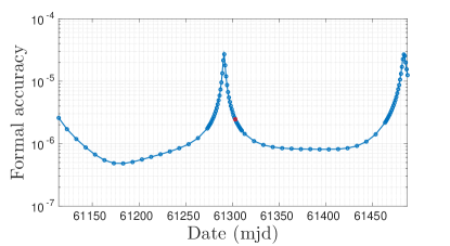
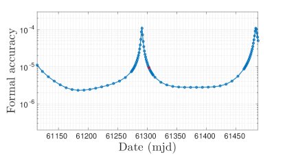
Figure 1: Formal accuracy of $\beta$ (left) and $\eta$ (right) as a function of the epoch of the estimate (in MJD) over the mission time span. In red the value of the accuracy for the estimate at central epoch.

The value of the formal accuracy at the central epoch (MJD 61303, corresponding to 20 September 2026) is highlighted in red. It is clear that there is a strong dependency of the achievable accuracy on the epoch of the estimate. If the planetary orbits are determined at MJD 61183 (23 May 2026), the accuracy of $\eta$ turns out to be $\sigma(\eta)\simeq 2.3\times 10^{-6}$, whereas estimating at MJD 61291 (8 September 2026) results in $\sigma(\eta)\simeq 1.1\times 10^{-4}$, almost two orders of magnitude larger. On the contrary, the uncertainty of the other PN parameters showed very little variability with the epoch of the estimate.

Such behaviour indicates the presence of some weak directions in orbit determination, possibly connected to the strategy adopted until now for the MORE Relativity Experiment: we determine only 8 out of 12 components of the initial conditions of Mercury and EMB. This assumption, first introduced in [19], is a solution to the presence of an approximate rank deficiency of order 4, arising when we try to determine the orbits of Mercury and the Earth (or, similarly, the EMB as in our problem) w.r.t. the Sun only by means of relative observations. Indeed, if there were only the Sun, Mercury and the Earth, and the Sun was perfectly spherical ($J_{2\odot}=0$), there would be an exact symmetry of order 3 represented by the rotation group $SO(3)$ applied to the state vectors of Mercury and the Earth. Because of the coupling with the other planets and due to the non-zero oblateness of the Sun, the symmetry is broken but only by a small amount, of the order of the relative size of the perturbations of the other planets on the orbits of Mercury and the Earth and of the order of $J_{2\odot}$.

Moreover, there is another approximate symmetry for scaling. The symmetry would be exact if there were only the Sun, Mercury and the Earth: if we change all the lengths involved in the problem by a factor $\lambda$, all the masses by a factor $\mu$ and all the times by a factor $\tau$, with the factors related by $\lambda^{3}=\tau^{2}\mu$ (Kepler’s third law), then the equation of motion of the gravitational 3-body problem would remain unchanged. Since we can assume that $\tau=1$, the symmetry for scaling involves the state vectors of Mercury and the Earth (i.e. the “lengths” involved in the problem) and the gravitational mass of the Sun, which is among the solve-for parameters. The symmetry for scaling can also be expressed by the well known fact that it is not possible to solve simultaneously for the mass of the Sun and the value of the astronomical unit. Since the state vectors of the other planets, perturbing the orbits of Mercury and the Earth, are given by the planetary ephemerides and thus they cannot be rescaled, the symmetry is broken but, again, only by a small amount. In conclusion, an approximate rank deficiency of order 4 occurs in the orbit determination problem we want to solve. Solving for all the 12 components of the initial conditions and the mass of the Sun would result in considerable loss of accuracy for all the parameters of the relativity experiment, as will be quantified in Sect. 4.

The only solution in case of rank deficiency is to change the problem. When no additional observations breaking the symmetry are available, a convenient solution is to remove some parameters from the solve-for list. Starting from $N$ parameters to be solved, in case of a rank deficiency of order $d$, we can select a new set of $N-d$ parameters to be solved, in such a way that the new normal matrix $\bar{C}$, with dimensions $(N-d)\times(N-d)$ instead of $N\times N$, has rank $N-d$. The remaining $d$ parameters can be set at some nominal value (consider parameters). This solution has been applied up to now in the MORE relativity experiment (see, e.g., [32]): the three position components and the out-of-plane velocity component of the EMB orbit, for a total of 4 parameters, have been removed from the solve-for list, curing in this way the rank deficiency of order 4.

Another option can be investigated: the use of a priori observations. When some information on one or more of the parameters involved in the symmetry is already available – for instance from previous experiments – it can be taken into account in our experiment and could lead to an improvement of the results. In this case the search for the minimum of the target function is restricted to the vector of parameters fulfilling a set of a priori equations. In practice, we add to the observations a set of a priori constraints, $\mathbf{u}=\mathbf{u}^{P}$, on the value of the parameters, with given a priori standard deviation $\sigma_{i}$ ($i=1,..N$) on each constraint $u_{i}=u_{i}^{P}$. This is equivalent to add to the normal equation in Eq. (1) an a priori normal equation of the form:

$$C^{P}\mathbf{u}=C^{P}\mathbf{u}^{P}\,,$$

with $C^{P}=\mbox{diag}[\sigma_{i}^{-1}]$. In this way, an “a priori penalty” is added to the target function:

$$Q(\mathbf{u})=\frac{1}{N+m}[(\mathbf{u}-\mathbf{u}^{P})^{T}C^{P}(\mathbf{u}-\mathbf{u}^{P})+\boldsymbol{\xi}^{T}(\mathbf{u})W\boldsymbol{\xi}(\mathbf{u})]$$

and the complete normal equation becomes:

$$(C^{P}+C)\Delta\mathbf{u}=-B^{T}W\boldsymbol{\xi}+C^{P}(\mathbf{u}^{P}-\mathbf{u}_{k})\,.$$

If the a priori uncertainties $\sigma_{i}$ are small enough, the new normal matrix $\bar{C}=C^{P}+C$ has rank $N$ and the complete orbit determination problem can be solved.

In our problem, the a priori information is represented by four constraint equations which inhibit the symmetry for rotation and scaling, to be added to the LS fit as a priori observations. A complete description of the form that the constraint equations assume will be given in Sect. 3.1.

2.4 The solar Lense-Thirring effect

In [32] we pointed out that the Lense-Thirring (LT) effect on the orbit of Mercury due to the angular momentum of the Sun has been neglected, in order to simplify the development and implementation of the dynamical model. In fact the solar LT effect is expected to be relevant at the level of accuracy of our tests [12]. As it will be clear in Sect. 4.2, the mismodelling resulting from neglecting this effect affects specifically the determination of the oblateness of the Sun, $J_{2\odot}$.

More specifically, the general relativistic LT effect induces a precession of the argument of the pericenter of Mercury in the gravity field of the Sun at the level of $\dot{\omega}_{\mathrm{LT}}=-2\,$milliarcsec/century, according to GR [15]. We modelled the effect as an additional perturbative acceleration in the heliocentric equation of motion of Mercury (see, e.g. [22]):

$$\mathbf{a}_{\mathrm{LT}}=\frac{(1+\gamma)\,GS_{\odot}}{c^{2}\,r^{3}}\left[-\hat{\mathbf{s}}\times\dot{\mathbf{r}}+3\,\frac{(\hat{\mathbf{s}}\cdot\mathbf{r})\,(\mathbf{r}\times\dot{\mathbf{r}})}{r^{2}}\right]\,,$$ (2)

where $\mathbf{S}_{\odot}=S_{\odot}\hat{\mathbf{s}}$ is the angular momentum of the Sun ($\hat{\mathbf{s}}$ is assumed along the rotation axis of the Sun). To assess the role of the solar LT in the dynamics, in Figure 2 we plot the effect of the solar LT acceleration, given by Eq. (2), on the simulated range of the orbiter. In other words, this is the difference between simulated range with and without LT effect over the one-year mission time span. As it can be seen, the mismodelling due to the lack of the solar LT perturbation in the dynamical model can be as high as some meters. This result is in very good agreement with Fig. 1 in [12], which shows the numerically integrated EMB-Mercury ranges with and without the perturbation due to the solar Lense-Thirring field over two years in the ICRF/J2000.0 reference frame, with the mean equinox of the reference epoch and the reference $x-y$ plane rotated from the mean ecliptic of the epoch to the Sun’s equator, centered at the SSB.

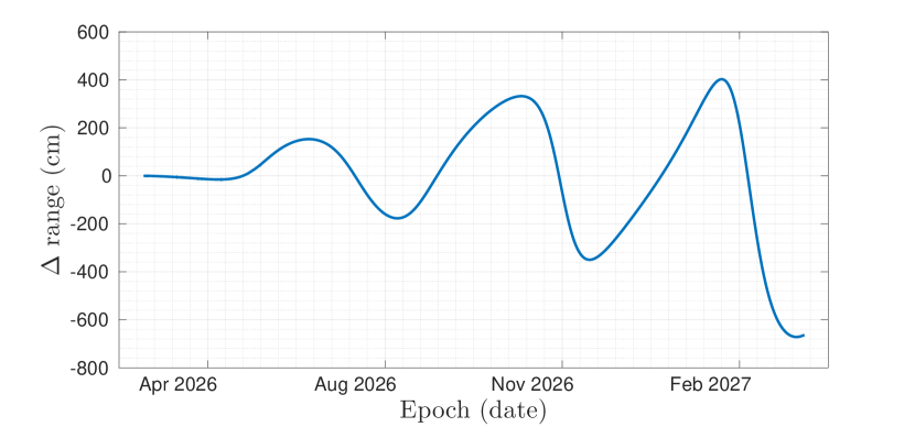
Figure 2: Difference (in cm) of simulated spacecraft range with and without solar LT perturbation in the dynamical model, over one-year mission time span.

3 The ORBIT14 software

Since 2007, the Celestial Mechanics Group of the University of Pisa has developed a complete software, ORBIT14, dedicated to the BepiColombo and Juno radio science experiments [38, 35], which is now ready for use. All the code is written in Fortran90. The software includes a data simulator, which generates the simulated observables and the nominal value for the orbital elements of the Mercury-centric orbit of the MPO and the heliocentric orbits of Mercury and the EMB, and the differential corrector, which is the core of the code, solving for the parameters of interest by a global non-linear LS fit, within a constrained multi-arc strategy [1]. The general structure of the software is described, e.g., in [32].

3.1 Handling the a priori constraints

The equations needed to a priori constrain the LS solution are given as an input to the differential corrector. In general, the $n$-th constraint has the expression: $f_{n}(\mathbf{u})=0$. ORBIT14 has been designed to handle only linear constraints. Thus, the equation for the $n$-th constraint, involving $d$ parameters to be determined, reads:

$$f_{n}(\mathbf{u})=\sum_{i=1}^{d}a_{i}(x_{i}-\theta_{i})=N(0,\mbox{diag}[\sigma_{i}])\,,$$

where $\sigma_{i}$ are the weights associated to each parameter involved in the constraint, assuming a Gaussian distribution with zero mean. Following the notation of Sect. 2.3, its contribution to the normal matrix is given by:

$$C_{n}^{P}=\left(\frac{\partial f_{n}}{\partial\mathbf{u}}\right)^{T}\,W\,\frac{\partial f_{n}}{\partial\mathbf{u}}\,,$$

and to the right hand side of the equations of motion by:

$$D_{n}^{P}=\left(\frac{\partial f_{n}}{\partial\mathbf{u}}\right)^{T}\,W\,f_{n}\,,$$

where $W=\mbox{diag}[\sigma_{i}^{-2}]$

In order to write the linear constraint equations of our orbit determination problem, let us introduce the following notation for the components of the state vectors of Mercury and the EMB:

• $\bf{M}$, $\dot{\bf{M}}$: position and velocity of Mercury at the reference epoch from ephemerides (nominal values); $\bf{m}$, $\dot{\bf{m}}$: estimated position and velocity of Mercury; $\Delta\bf{M}=\bf{M}-\bf{m}$, $\Delta\dot{\bf{M}}=\dot{\bf{M}}-\dot{\bf{m}}$: deviation between ephemerides and estimate.

• $\bf{E}$, $\dot{\bf{E}}$: position and velocity of EMB at the reference epoch from ephemerides; $\bf{e}$, $\dot{\bf{e}}$: estimated position and velocity of EMB; $\Delta\bf{E}=\bf{E}-\bf{e}$, $\Delta\dot{\bf{E}}=\dot{\bf{E}}-\dot{\bf{e}}$: deviation between ephemerides and estimate.

Symmetry for rotations.

The symmetry for rotation is described by a three-parameter group, whose generators are for example the rotations around three orthogonal axis $(x,y,z)$ of the reference frame used for orbit propagation. The constraint equation which inhibits an infinitesimal rotation by an angle $s$ around the $x$-axis has the expression:

$$\begin{split}&\left.\frac{\Delta\mathbf{M}}{|\mathbf{m}|}\cdot\frac{\partial(R_{s,\hat{x}}\hat{\mathbf{M}})}{\partial s}\right\arrowvert_{s=0}+\left.\frac{\Delta\mathbf{E}}{|\mathbf{e}|}\cdot\frac{\partial(R_{s,\hat{x}}\hat{\mathbf{E}})}{\partial s}\right\arrowvert_{s=0}+\left.\frac{\Delta\dot{\mathbf{M}}}{|\dot{\mathbf{m}}|}\cdot\frac{\partial(R_{s,\hat{x}}\hat{\dot{\mathbf{M}}})}{\partial s}\right\arrowvert_{s=0}+\\ &+\left.\frac{\Delta\dot{\mathbf{E}}}{|\dot{\mathbf{e}}|}\cdot\frac{\partial(R_{s,\hat{x}}\hat{\dot{\mathbf{E}}})}{\partial s}\right\arrowvert_{s=0}=N(\mbox{diag}[\sigma_{i}],0)\,,\end{split}$$ (3)

where $\sigma_{i}$ are the weights for the state vectors components, $N$ represents a Gaussian distribution with zero mean, $R_{s,\hat{x}}$ is the rotation matrix by an angle $s$ around the $x$-axis:

$$R_{s,\hat{x}}=\begin{pmatrix}1&0&0\\ 0&\cos s&-\sin s\\ 0&\sin s&\cos s\\ \end{pmatrix}$$

and $(\partial R_{s}/\partial s)\arrowvert_{s=0}$ is a generator of the Lie algebra of the rotations $SO(3)$. Two similar equations hold for the rotations by an angle $s$ around the $y$ and $z$ axes.

Symmetry for scaling.

To find the equation to constrain for scaling, we can start from the simple planar two-body problem of a planet around the Sun, with the non-linear dependency of the mean motion $n$ upon the semi-major axis $a$, in the hypothesis of circular motion:

$$\frac{da}{dt}=0,\,\,\,\,\,\frac{d\lambda}{dt}=n(a)=\frac{k}{a^{3/2}}\,,$$ (4)

where $k^{2}=GM_{\odot}=\mu_{\odot}$, with solution given by:

$$a(t)=a_{0},\,\,\,\,\,\lambda(t)=\frac{k}{a_{0}^{3/2}}t+\lambda_{0}\,.$$ (5)

This problem has a symmetry with multiplicative parameter $w\in\mathbb{R}^{+}$:

$$k\mapsto w^{3}k,\,\,\,\,\,a_{0}\mapsto w^{2}a_{0}\,,$$ (6)

leaving $n=k/a^{3/2}$ invariant. The symmetry can be represented by means of an additive parameter $s$ by setting $w=e^{s}$. The derivative of the symmetry group action with respect to $s$ is:

$$\frac{da_{0}}{ds}=2w^{2}a_{0},\,\,\,\,\,\frac{dk}{ds}=3w^{3}k\,.$$ (7)

Finally, the constraint takes the form:

$$-3\,\frac{\Delta a}{a_{0}}\,\left.\frac{da_{0}}{ds}\right\arrowvert_{s=0}+2\,\frac{\Delta k}{k_{0}}\,\left.\frac{dk}{ds}\right\arrowvert_{s=0}=0\,.$$ (8)

In our fit, we estimate the parameter $\mu_{\odot}$, that is $k^{1/2}$. Since we need to deal with linear constraints, we can linearize the problem by expanding the non-linear equation up to the first order around the nominal value. In this way, the final expression adopted for the scaling constraint reads:

$$\sum_{j=1}^{3}\left[\frac{\Delta M_{j}}{|\mathbf{M}|}\,M_{j}+\frac{\Delta\dot{M}_{j}}{|\dot{\mathbf{M}}|}\,\dot{M}_{j}+\frac{\Delta E_{j}}{|\mathbf{E}|}\,E_{j}+\frac{\Delta\dot{E}_{j}}{|\dot{\mathbf{E}}|}\,\dot{E}_{j}\right]+3\Delta\mu_{\odot}=N(\mbox{diag}[\sigma_{i}],0)\,,$$ (9)

where $j=1,2,3$ refers to the three orthogonal directions $x,y,z$.

Setting the weights $\sigma_{i}$.

Together with the constraint equations given in input to the differential corrector, it is necessary to provide also the a priori standard deviations $\sigma_{i}$ by which the involved parameters are constrained. The strength of the weights $\sigma_{i}$ is the result of a trade-off between two opposite trends: on the one hand, the tighter the constraint the less the solution is affected by the corresponding rank deficiency; on the other hand, if the constraint is too tight, the approach becomes equivalent to descoping, i.e. the involved parameters are handled as consider parameters.

The formulation given in Eqs. (3) and (9) implies the employment of adimensional weights, which constrain the relative accuracy of each involved parameter. To find a suitable value for the weights, we start from a standard simulation of the relativity experiment, obtained by estimating only 8 out of the 12 components of the orbits of Mercury and the EMB, and we consider the ratio between the formal accuracy of each component and the corresponding estimated value. The results are shown in Table 1, where we included also the ratio of the accuracy over the estimated value of $\mu_{\odot}$.

Table 1: Ratio between the formal accuracy and the estimated value for the 8 components of Mercury and the EMB orbits and for $\mu_{\odot}$. All values are normalised to $10^{-12}$.

$\frac{\sigma(x_{M})}{x_{M}}$	$\frac{\sigma(y_{M})}{y_{M}}$	$\frac{\sigma(z_{M})}{z_{M}}$	$\frac{\sigma(\dot{x}_{M})}{\dot{x}_{M}}$	$\frac{\sigma(\dot{y}_{M})}{\dot{y}_{M}}$	$\frac{\sigma(\dot{z}_{M})}{\dot{z}_{M}}$	$\frac{\sigma(\dot{x}_{E})}{\dot{x}_{E}}$	$\frac{\sigma(\dot{y}_{E})}{\dot{y}_{E}}$	$\frac{\sigma(\mu_{\odot})}{\mu_{\odot}}$
$0.22$	$0.61$	$3.1$	$0.23$	$0.26$	$3.2$	$4.4$	$0.29$	$0.78$

All the values range between $10^{-12}$ and $10^{-13}$, thus suitable values to be adopted are $\sigma_{i}\sim 10^{-13}-10^{-14}$. In the following, we will adopt a relative weight $\sigma_{i}=10^{-14}$ for each parameter involved in the a priori constraints. Nevertheless, we checked that adopting $\sigma_{i}=10^{-13}$ for each parameter, the worsening of the global solution is negligible.

3.2 Simulation scenario

To perform a global simulation of the radio science experiment, we make use of some assumptions both at simulation stage and during the differential correction process, which are briefly described in the following.

Error models.

To simulate the observables in a realistic way, we need to make some assumptions concerning the error sources which unavoidably affect the observations. We assume that the radio tracking observables are affected only by random effects with a standard deviation of $\sigma_{r}=15\,$cm at 300 s and $\sigma_{\dot{r}}=1.5\times 10^{-4}\,$cm/s at 1000 s, respectively, for Ka-band observations. The software is capable of including also a possible systematic component to the range error model and to calibrate for it, but we did not account for this detrimental effect in the present work, which has been partially discussed in [31].

The accelerometer readings themselves suffer from errors of both random and systematic origin, which can significantly bias the results of the orbit determination. Systematic effects due to the accelerometer readings turn out to be particularly detrimental for the purposes of gravimetry and rotation (see, e.g., the discussion in [6]), while they induce a minor loss in accuracy for what concerns the relativity experiment (see, e.g., [29] and [31]). The adopted accelerometer error model, provided by the ISA team (private communications) and the digital calibration method applied during the differential correction process have been extensively discussed in [6].

Additional rank deficiencies in the problem.

A critical issue which significantly affects the success of the relativity experiment concerns the high correlation between the Eddington parameter $\beta$ and the solar oblateness $J_{2\odot}$. Indeed, from a geometrical point of view the main orbital effect of $\beta$ is a precession of the argument of perihelion, which is a displacement taking place in the plane of the orbit of Mercury, while $J_{2\odot}$ affects the precession of the longitude of the node, producing a displacement in the plane of the solar equator. Since the angle between the two planes is almost zero, the two effects blend each other and the parameters turn out to be highly correlated, causing a deterioration of the solution. A meaningful solution to the problem is to link the PN parameters through the Nordtvedt equation [24]:

$$\eta=4(\beta-1)-(\gamma-1)-\alpha_{1}-\frac{2}{3}\alpha_{2}\,$$ (10)

and add such relation as an a priori constraint to the LS fit. In such a way, the knowledge of $\beta$ is mainly determined from the value of $\eta$ and $\gamma$, removing the correlation with $J_{2\odot}$. This assumption corresponds to hypothesise that gravity is a metric theory.

Moreover, a solar superior conjunction experiment (SCE) for the determination of the PN parameter $\gamma$ is expected during the cruise phase of the BepiColombo mission (see, e.g., the description in [19]), similar to the one performed by Cassini [4]. The resulting estimate of $\gamma$ will be adopted as an a priori constraint on the parameter in the experiment in orbit. The complete results and a thorough discussion on the simulations of SCE with ORBIT14 will be presented in a future paper; however, we include in the fit a constraint on the value of $\gamma$ given by: $\gamma=1\pm 5\times 10^{-6}$, coming from our cruise simulations. In this way, from Eq. (10) it turns out that $\beta$ is mainly determined from $\eta$, with a ratio $1:4$ in the corresponding accuracies and a near-one correlation between the two parameters. Indeed, this fact was already clear from Fig. 1: the accuracy of the two parameters shows exactly the same behaviour as a function of the epoch of the estimate and, at each given epoch, the ratio of the accuracies is around 4.

Solve-for list.

The latest mission scenario consists of a one-year orbital phase, with a possible extension to another year, starting from 15 March 2026. The orbital elements of the initial Mercury-centric orbit of the MPO orbiter are:

$$1500\times 480\,\mbox{km},\,\,\,i=90^{\circ},\,\,\,\Omega=67.8^{\circ},\,\,\,\omega=16^{\circ}.$$

We assume that only one ground station is available for tracking, at the Goldstone Deep Space Communications Complex in California (USA), providing observations in the Ka-band. We solved for a total of almost 5000 parameters simultaneously in the non-linear LS fit adopting a constrained multi-arc strategy and accounting for the correlations. The list of solve-for parameters includes:

• state vector (position and velocity) of the Mercury-centric orbit of the spacecraft at each arc and of Mercury and Earth-Moon barycenter at the central epoch of the mission, in the Ecliptic Reference frame at epoch J2000;

• the PN parameters $\beta$, $\gamma$, $\eta$, $\alpha_{1}$, $\alpha_{2}$ and the related parameters $J_{2\odot}$, $\mu_{\odot}$, $\zeta$ and $GS_{\odot}$ of the Sun;

• the calibration coefficients for the accelerometer readings at each arc (six parameters per arc).

4 Numerical results

In this Section we describe the results of the numerical simulations of the MORE relativity experiment. In Sect. 4.1 we compare the two possible strategies described in Sect. 2.3 to remove the rank deficiency of order 4 due to the symmetry for rotation and scaling. Then, in Sect. 4.2 we discuss the effects on the solution due to the addition of the solar LT effect in the dynamical model, with a particular attention on the estimate of $J_{2\odot}$.

4.1 Removing the planetary rank deficiency

We briefly recall the two possible strategies to remove the approximate rank deficiency of order 4 found when we try to solve simultaneously for the orbits of Mercury and the EMB (12 parameters) and the solar gravitational mass $\mu_{\odot}$:

• strategy I (descoping): we remove 4 out of the 13 parameters from the solve-for list (the three position components of the EMB and the $z$-component of the velocity of the EMB);

• strategy II: we solve simultaneously for the 13 parameters by adding 4 a priori constraint equations in the LS fit.

In Table 2 the expected accuracies for the PN and related parameters obtained following both strategies are compared with the current knowledge of the same parameters. Table 3 provides the achievable accuracies for the state vectors components. For all parameters, the reference date for the estimate is the central epoch of the mission. In both tables, the last column contains the accuracies that would be obtained if all the state vectors components and $\mu_{\odot}$ are determined simultaneously without any a priori constraint whatsoever. Because of the approximate rank deficiency of order 4 (described in Sect. 2.3), the normal matrix is still invertible, yet the global solution is highly downgraded. We note indeed a loss in accuracy up to 2-3 orders of magnitude in the components of the planetary state vectors, while an order of magnitude is lost in the solution for $\beta$ and $\eta$. As far as the other relativistic parameters are concerned, it turns out that knowing the orbits of Mercury and the EMB at the level of some meters is sufficient to determine their value at the goal level of accuracy of MORE.

Table 2: Comparison of the accuracies of PN and related parameters following the two possible strategies; the fourth column contains the current knowledge of each parameter; the last column shows the solution achieved by solving for all the parameters without a priori constraints on Mercury and EMB state vector. The accuracy of $\mu_{\odot}$ is in cm³/s², of $\zeta$ in y^-1.

Parameter	Strategy I	Strategy II	Current knowledge	No constraints
$\beta$	$2.4\times 10^{-6}$	$2.9\times 10^{-6}$	$7\times 10^{-5}$[8],$\ 3.9\times 10^{-5}$[25]	$2.7\times 10^{-5}$
$\gamma$	$7.6\times 10^{-7}$	$7.6\times 10^{-7}$	$2.3\times 10^{-5}$[4]	$\ 7.7\times 10^{-7}$
$\eta$	$9.3\times 10^{-6}$	$1.1\times 10^{-5}$	$4.5\times 10^{-4}$[41]	$1.1\times 10^{-4}$
$\alpha_{1}$	$4.9\times 10^{-7}$	$4.8\times 10^{-7}$	$6.0\times 10^{-6}$[14]	$7.5\times 10^{-7}$
$\alpha_{2}$	$1.1\times 10^{-7}$	$1.1\times 10^{-7}$	$3.5\times 10^{-5}$[14]	$1.2\times 10^{-7}$
$\mu_{\odot}$	$1.0\times 10^{14}$	$1.1\times 10^{14}$	$8\times 10^{15}$ [42]	$1.9\times 10^{14}$
$J_{2\odot}$	$4.9\times 10^{-9}$	$5.0\times 10^{-9}$	$1.2\times 10^{-8}$[8],$\,9\times 10^{-9}$[25]	$5.5\times 10^{-9}$
$\zeta$	$3.2\times 10^{-14}$	$3.3\times 10^{-14}$	$4.3\times 10^{-14}$ [27]	$3.5\times 10^{-14}$

Table 3: Comparison of the accuracies of the state vectors components following the two possible strategies and solving for all the parameters without a priori constraints. Accuracies in position are in cm, in velocity in cm/s.

Parameter	Strategy I	Strategy II	No constraints
$x_{M}$	0.81	0.65	$4.50\times 10^{2}$
$y_{M}$	3.6	3.0	$2.68\times 10^{2}$
$z_{M}$	4.2	2.2	$1.633\times 10^{3}$
$x_{E}$	–	0.70	$5.89\times 10^{1}$
$y_{E}$	–	2.8	$1.093\times 10^{3}$
$z_{E}$	–	4.3	$4.275\times 10^{3}$
$\dot{x}_{M}$	$7.3\times 10^{-7}$	$3.6\times 10^{-7}$	$2.83\times 10^{-4}$
$\dot{y}_{M}$	$6.1\times 10^{-7}$	$2.4\times 10^{-7}$	$2.58\times 10^{-4}$
$\dot{z}_{M}$	$1.5\times 10^{-6}$	$8.1\times 10^{-7}$	$1.01\times 10^{-3}$
$\dot{x}_{E}$	$5.0\times 10^{-7}$	$1.2\times 10^{-7}$	$2.16\times 10^{-4}$
$\dot{y}_{E}$	$8.6\times 10^{-7}$	$9.2\times 10^{-7}$	$8.26\times 10^{-6}$
$\dot{z}_{E}$	–	$7.3\times 10^{-7}$	$6.27\times 10^{-4}$

The results achievable with strategies I and II are almost comparable and represent a significant improvement with respect to the current knowledge (see the discussion in [32] for a comparison with the actual knowledge). This is true if orbit determination is performed at the central epoch of the orbital mission. Indeed, from Fig. 1 we have seen that, adopting strategy I, there is a strong dependency of the solution from the epoch. In Fig. 3 we compare the behaviour of the formal accuracy of $\beta$ (on the left) and $\eta$ (on the right) adopting strategy I (blue curve) and strategy II (green curve). The red circle refers to the estimate at the central epoch (MJD 61303).

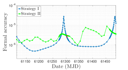
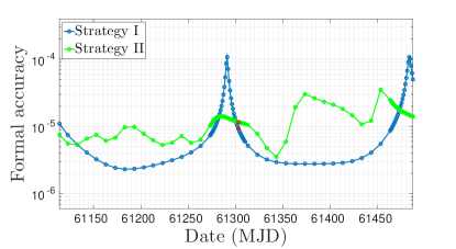
Figure 3: Comparison of the formal accuracy of $\beta$ (left) and $\eta$ (right) as a function of the epoch of the estimate (in MJD) over the mission time span adopting strategy I (blue curve) and strategy II (green curve). In red the value of the accuracy for the estimate at central epoch.

Choosing the second strategy, we observe that the dependency of the accuracy from the epoch of the estimate is definitely reduced. If we consider the evolution of the formal of $\eta$ from the beginning of the orbital mission up to MJD 61350, the variability in case of strategy I spans from a minimum of $\sigma(\eta)=2.3\times 10^{-6}$ to a maximum of $\sigma(\eta)=1.1\times 10^{-4}$, while adopting strategy II the formal accuracy ranges from a minimum of $\sigma(\eta)=3.5\times 10^{-6}$ to a maximum of $\sigma(\eta)=1.4\times 10^{-5}$, with a net variability of only a factor 4 instead of a factor 50. If the orbits of Mercury and the EMB are determined in the second part of the mission, we observe a stronger variability in the accuracies adopting the second approach. Such behaviour could suggest that some degeneracy is still affecting the orbit determination problem. This issue will be investigated in the future. Nevertheless, the standard strategy of orbit determination codes is to adopt, as the reference epoch, the initial or the central date, thus for the purpose of our simulations we can ignore the behaviour of the curves in the second half of the mission time span.

Of course, if the mission scenario is exactly the one adopted in our simulations, i.e. assuming the beginning of scientific operations on 15 March 2026 and the end on 21 March 2027 (corresponding to 365 observed arcs), choosing strategy I or II does not lead to significant differences in the solution. However, Fig. 3 states that strategy II provides a more stable solution. Indeed, as an example, in Table 4 we show the results for the accuracy of relativity parameters in the hypothesis of moving up the beginning of the orbital experiment by approximately two weeks, on 3 March 2026, still keeping the one-year duration.

Table 4: Comparison of the accuracies of PN and related parameters following the two possible strategies in the hypothesis of beginning of scientific operations in orbit on 3 March 2026 instead of 15 March 2026. The last two columns show the ratio of accuracy attained, for each parameter, on the scenario of 3 March over that achieved on the scenario of 15 March, in the case of strategy I and II, respectively. The accuracy of $\mu_{\odot}$ is in cm³/s², of $\zeta$ in y^-1.

Parameter	Strategy I	Strategy II	Ratio I	Ratio II
$\beta$	$3.0\times 10^{-5}$	$2.3\times 10^{-6}$	$12.5$	$0.79$
$\gamma$	$6.4\times 10^{-7}$	$7.7\times 10^{-7}$	$0.84$	$1.0$
$\eta$	$1.2\times 10^{-4}$	$8.7\times 10^{-6}$	$12.5$	$0.79$
$\alpha_{1}$	$7.6\times 10^{-7}$	$4.4\times 10^{-7}$	$1.5$	$0.92$
$\alpha_{2}$	$9.6\times 10^{-8}$	$8.0\times 10^{-8}$	$0.87$	$0.73$
$\mu_{\odot}$	$1.8\times 10^{14}$	$7.9\times 10^{13}$	$1.8$	$0.72$
$J_{2\odot}$	$4.7\times 10^{-9}$	$4.3\times 10^{-9}$	$0.9$	$0.86$
$\zeta$	$2.6\times 10^{-14}$	$2.7\times 10^{-14}$	$0.81$	$0.82$

The last two columns of Table 4 shows the ratio between the accuracy achieved for each parameter in the scenario of 3 March 2026 and the one of the 15 March 2026 scenario, for strategies I and II, respectively. It is clear that adopting the second approach, a slight variation in the initial date of the mission in orbit leads only to slight variations in the accuracy of the relativity parameters, as it has to be. Conversely, in the case of the first strategy the solution turns out to be less stable. Indeed, the accuracy of $\beta$ and $\eta$ varies by an order of magnitude between the two scenarios, weakening the reliability of the achieved results.

For completeness, Table 5 shows the correlations between PN and related parameters in the case of strategy I (top) and strategy II (bottom). Values higher than 0.8 have been highlighted.

Table 5: Correlations between PN and related parameters in the case of strategy I (top) and strategy II (bottom). Values higher than 0.8 have been highlighted.

	$\beta$	$\gamma$	$\eta$	$\alpha_{1}$	$\alpha_{2}$	$\mu_{\odot}$	$J_{2\odot}$	$\zeta$
$\zeta$	$<0.1$	$0.12$	$<0.1$	$0.12$	$0.49$	$0.74$	$0.76$	–
$J_{2\odot}$	$<0.1$	$<0.1$	$<0.1$	$<0.1$	$0.26$	$\mathbf{0.86}$	–
$\mu_{\odot}$	$0.22$	$<0.1$	$0.22$	$0.42$	$0.38$	–
$\alpha_{2}$	$0.44$	$0.14$	$0.46$	$0.28$	–
$\alpha_{1}$	$0.25$	$0.12$	$0.21$	–
$\eta$	$\mathbf{0.99}$	$0.56$	–
$\gamma$	$0.62$	–
$\beta$	–
	$\beta$	$\gamma$	$\eta$	$\alpha_{1}$	$\alpha_{2}$	$\mu_{\odot}$	$J_{2\odot}$	$\zeta$
$\zeta$	$0.63$	$0.11$	$0.64$	$<0.1$	$0.51$	$0.76$	$0.77$	–
$J_{2\odot}$	$0.54$	$<0.1$	$0.55$	$0.11$	$0.29$	$\mathbf{0.86}$	–
$\mu_{\odot}$	$0.76$	$<0.1$	$0.76$	$0.35$	$0.42$	–
$\alpha_{2}$	$0.73$	$0.13$	$0.73$	$0.24$	–
$\alpha_{1}$	$0.36$	$0.17$	$0.31$	–
$\eta$	$\mathbf{0.99}$	$<0.1$	–
$\gamma$	$0.16$	–
$\beta$	–

In both cases we find a high correlation only between the two physical parameters of the Sun, i.e. $\mu_{\odot}$ and $J_{2\odot}$, and between $\beta$ and $\eta$, whose correlation is near 1 due to the assumption that PN parameters are linked through the Nordtvedt equation. In general, correlations between the parameters, although restrained, are higher in the case of strategy II. This fact was expected since, from Table 2, formal accuracies at the central epoch are slightly worse than adopting strategy I. Nevertheless, except the correlation between $\mu_{\odot}$-$J_{2\odot}$ and $\beta$-$\eta$, they are always lower than 0.8.

4.2 Solar LT effect and the determination of $J_{2\odot}$

In Sect. 2.4 we showed that the solar LT effect on Mercury produces a signal with a peak-to-peak amplitude up to about ten meters after one year, hence it should be taken into account in the BepiColombo radio science data processing, otherwise it would alias the recovery of other effects, as already pointed out in [12]. In that paper it was also underlined that the measurement of the solar quadrupole $J_{2\odot}$ at the $1\%$ level or better, which is one of the goals of MORE, cannot be performed aside from accounting for the solar LT effect; the impact of neglecting the gravitomagnetic field of the Sun may affect indeed the determination of $J_{2\odot}$ at the $12\%$ level. Moreover, in [25] the authors observe that, processing three years of ranging data to MESSENGER by explicitly modelling the gravitomagnetic field of the Sun, the small precession of the perihelion of Mercury induced by solar LT turns out to be highly correlated with the precession due to $J_{2\odot}$.

In this section we investigate two different aspects of the problem with BepiColombo MORE: firstly, we measure the impact on the estimated value of $J_{2\odot}$ if we do not include the solar LT in the dynamical model; secondly, we check whether solving for $GS_{\odot}$ introduces some weakness in the orbit determination problem, for instance deteriorating the formal uncertainties of the other parameters, especially $J_{2\odot}$.

In order to address the first matter, we simulated one year of BepiColombo observations including the solar LT effect and then we applied the differential corrections in two different cases: (i) we included solar LT in the corrector model; (ii) we did not include solar LT in differential corrections. The set of estimated parameters is the same of Sect 3.2, except for the solar angular momentum, which is assumed at the nominal value $S_{\odot}=1.92\times 10^{48}\,$g cm²/s [13]. The results for the estimated value and formal accuracy of $J_{2\odot}$ in the two cases are shown in Table 6.

Table 6: Estimated value and formal accuracy of $J_{2\odot}$ with solar LT on and off, respectively, in differential correction stage. The parameter $GS_{\odot}$ is not determined and it is assumed at its nominal value.

Case	Estimated value	$\sigma(J_{2\odot})$
LT ON	$1.992\times 10^{-7}$	$6.0\times 10^{-10}$
LT OFF	$1.837\times 10^{-7}$	$6.0\times 10^{-10}$

As expected, the formal accuracy is the same in both cases, while the estimated value of $J_{2\odot}$ at convergence is different. More precisely, we observe that neglecting the solar LT effect on the orbit of Mercury (second simulation) introduces a bias in the estimated value of $J_{2\odot}$ as large as $27\sigma$. The effect on the other parameters is only marginally relevant: we remarked a bias in $\mu_{\odot}$ of $\sim 5\sigma$ and in some components of the orbit of Mercury, of the same amount. On the contrary, in the first simulation the estimated value of $J_{2\odot}$ lies within $1.3\sigma$ with respect to the nominal value. In conclusion, this test confirms that the solar LT acceleration produces effects on the orbit of Mercury which can be absorbed by $J_{2\odot}$, if not properly modelled. Under no circumstances should the LT effect be neglected for the BepiColombo MORE experiment.

Now that we proved that it is crucial to include the gravitomagnetic acceleration due to the Sun in the dynamical model, we go on to discuss the second point. We introduce the Lense-Thirring parameter $GS_{\odot}$ in the solve-for list: due to the high correlation with $J_{2\odot}$, we expect to find a significant worsening in the solution for the solar oblateness. A similar behaviour was already found in the case of the mission Juno and described in [35]. We considered three explanatory cases: (i) $J_{2\odot}$ and $GS_{\odot}$ are determined simultaneously without any a priori information on their values (same setup of Sect. 3.2); (ii) the value of $J_{2\odot}$ is a priori constrained to its present knowledge $2\pm 0.12\times 10^{-7}$ (cf. [8]); (iii) the value of $GS_{\odot}$ is a priori constrained to $10\%$ level.

Table 7: Achievable accuracy on $J_{2\odot}$ and correlation with $GS_{\odot}$ in the following cases: (i) $J_{2\odot}$ and $GS_{\odot}$ are determined assuming no a priori information on their value; (ii) $J_{2\odot}$ is constrained to the a priori value $2\pm 0.12\times 10^{-7}$ (present knowledge); (iii) $GS_{\odot}$ is a priori constrained to $10\%$ of its value.

	Case (i)	Case (ii)	Case (iii)
$\sigma(J_{2\odot})$	$5.0\times 10^{-9}$	$4.6\times 10^{-9}$	$1.7\times 10^{-9}$
correlation with $GS_{\odot}$	0.9928	0.9919	0.9354

The results are shown in Table 7. The simultaneous determination of $J_{2\odot}$ and $GS_{\odot}$ without any a priori (case (i)) leads to a 0.99 correlation between the two parameters, as expected. As a result, the solution with respect to the first row of Table 6 is downgraded by almost an order of magnitude. Add an a priori on $J_{2\odot}$ at the level of the current knowledge (case (ii)) does not change much the result, as the correlation between $J_{2\odot}$ and $GS_{\odot}$ does not decrease significantly. Conversely, a rather weak constraint on $GS_{\odot}$ (case (iii)) is capable of significantly improving the solution, breaking the correlation between the two parameters (from 0.99 to 0.93). A tighter constraint on $GS_{\odot}$ would provide a further improvement of the results. As a conclusion, we can state that the achievable accuracy on $J_{2\odot}$ will be mainly limited by the knowledge of the solar angular momentum.

5 Conclusions and remarks

The present paper addresses two critical aspects of the BepiColombo relativity experiment we aim to solve. The first one concerns the approximate rank deficiency of order 4 found in the Earth and Mercury orbit determination problem. In particular, we highlighted that, according on how the rank deficiency is cured, the dependency of the PN parameters $\beta$ and $\eta$ from the epoch of the estimate can be highly pronounced. As a consequence, the reliability of the solution can be compromised. We considered two possible strategies: the set of 13 critical parameters (initial conditions of Mercury and EMB and the gravitational mass of the Sun) can be reduced to only 9 parameters to be determined, as done up to now in the relativity experiment settings, or we can solve for the whole set of parameters providing 4 a priori constraint equations in input to the differential correction process. We concluded that, although by chance the present mission scenario does not imply considerable differences between the two strategies, the second strategy leads to a more stable solution and, thus, is the more advisable approach.

Secondly, we studied the impact on the determination of the solar oblateness parameter $J_{2\odot}$ of a failure to include the solar LT perturbation in Mercury’s dynamical model. The parameter $J_{2\odot}$ turns out to be highly correlated with the LT parameter $GS_{\odot}$, containing the solar angular momentum. We pointed out that neglecting the solar LT effect leads to a considerable bias in the estimated value of $J_{2\odot}$, and to an illusory high accuracy in the determination of the same parameter. Nevertheless, we have shown that including in the LS fit some reasonable a priori information on $GS_{\odot}$ can help contain the deterioration of the solution for $J_{2\odot}$.

The results of the research presented in this paper have been performed within the scope of the Addendum n. I/080/09/1 of the contract n. I/080/09/0 with the Italian Space Agency.

References

- [1] E.M. Alessi, S. Cicaló, A. Milani and G. Tommei, Desaturation manoeuvers and precise orbit determination for the BepiColombo mission, Mon. Not. R. Astron. Soc., 423, 2270-2278 (2012).
- [2] N. Ashby. P.L. Bender and J.M Wahr, Future gravitational physics tests from ranging to the BepiColombo Mercury planetary orbiter, Phys. Rev. D, 75, 022001 (2007).
- [3] J. Benkhoff et al., BepiColombo - Comprehensive exploration of Mercury: Mission overview and science goals, Plan. Space. Sci., 58, 2-10 (2010).
- [4] B. Bertotti, L. Iess and P. Tortora, A test of general relativity using radio links with the Cassini spacecraft, Nature, 425, 374-376 (2003).
- [5] S. Cicalò and A. Milani, Determination of the rotation of Mercury from satellite gravimetry, Mon. Not. R. Astron. Soc., 427, 468-482 (2012).
- [6] S. Cicalò et al., The BepiColombo MORE gravimetry and rotation experiments with the ORBIT14 software, Mon. Not. R. Astron. Soc., 457, 1507-1521 (2016).
- [7] F. De Marchi, G. Tommei, A. Milani and G. Schettino, Constraining the Nordtvedt parameter with the BepiColombo Radioscience experiment, Phys. Rev. D, 93, 1230014 (2016).
- [8] A. Fienga, J. Laskar, P. Exertier, H. Manche and M. Gastineus, Numerical estimation of the sensitivity of INPOP planetary ephemerides to general relativity parameters, Celest. Mech. Dyn. Astron., 123, 325-349 (2015).
- [9] V. Iafolla et al., Italian Spring Accelerometer (ISA): A fundamental support to BepiColombo Radio Science Experiments, Planet. Space Sci., 58 300-308, (2010).
- [10] L. Iess and G. Boscagli, Advanced radio science instrumentation for the mission BepiColombo to Mercury, Planet. Space Sci., 49, 1597-1608 (2001).
- [11] L. Iess, S. Asmar and P. Tortora, MORE: An advanced tracking experiment for the exploration of Mercury with the mission BepiColombo, Acta Astron., 65, 666-675 (2009).
- [12] L. Iorio, H.I.M. Lichtenegger, M.L. Ruggiero and C. Corda, Phenomenology of the Lense-Thirring effect in the solar system, Astrophys. Space Sci., 31, 351-395 (2011).
- [13] L. Iorio, Constraining the Angular Momentum of the Sun with Planetary Orbital Motions and General Relativity, Solar Phys., 281, 815–826 (2012).
- [14] L. Iorio, Constraining the Preferred-Frame , Parameters from Solar System Planetary Precessions , Int. J. Mod. Phys. D, 23, 1450006 (2014).
- [15] L. Iorio, arXiv:1601.01382 (2016).
- [16] Y. Kozai, Effects of the Tidal Deformation of the Earth on the Motion of Close Earth Satellites, Publ. Astron. Soc. Jpn., 17, 395-402 (1965).
- [17] J. Lense, H. Thirring, Über den Einflußder Eigenrotation der Zentralkörper auf die Bewegung der Planeten und Monde nach der Einsteinschen Gravitationstheorie, Phys. Z., 19, 156 (1918).
- [18] A. Milani et al., Gravity field and rotation state of Mercury from the BepiColombo Radio Science Experiments, Plan. Space Sci., 49, 1579-1596 (2001).
- [19] A. Milani et al., Testing general relativity with the BepiColombo radio science experiment, Phys. Rev. D, 66, 082001 (2002).
- [20] A. Milani et al., Relativistic models for the BepiColombo radioscience experiment, in Relativity in Fundamental Astronomy: Dynamics, Reference Frames, and Data Analysis, Proceedings of the International Astronomical Union, IAU Symposium, 261, 356-365 (2010).
- [21] A. Milani and G.F. Gronchi, Theory of orbit determination, Cambridge Univ. Press, Cambridge, UK (2010).
- [22] T.D. Moyer, Formulation for Observed and Computed Values of Deep Space Network Data Types of Navigation, NASA JPL, Deep Space Communications and Navigation Series, Monograph 2 (2000).
- [23] T. Mukai et al., Present status of the BepiColombo/Mercury magnetospheric orbiter, Adv. Space Res., 38 578-582 (2006).
- [24] K.J. Nordtvedt, Post-Newtonian Metric for a General Class of Scalar-Tensor Gravitational Theories and Observational Consequences, Astrophys. Journal, 161, 1059-1067 (1960).
- [25] R.S. Park et al., Precession of Mercury’s Perihelion from Ranging to the MESSENGER Spacecraft, Astron. J., 153, 121 1-7 (2017).
- [26] F.P. Pijpers, Helioseismic determination of the solar gravitational quadrupole moment, Mon. Not. R. Astron. Soc., 297, L76-L80 (1998).
- [27] E.V. Pitjeva and N.P. Pitjev, Relativistic effects and dark matter in the Solar system from observations of planets and spacecraft, Mon. Not. R. Astron. Soc., 432, 3431-3437 (2013).
- [28] N. Sanchez Ortiz, M. Belló Mora and R. Jehn, BepiColombo mission: Estimation of Mercury gravity field and rotation parameters, Acta Astron., 58, 236-242 (2006).
- [29] G. Schettino, S. Cicaló, S. Di Ruzza and G. Tommei, The relativity experiment of MORE: global full-cycle simulation and results, in Proceedings of the IEEE Metrology for Aerospace (MetroAeroSpace), Benevento, Italy, 2015, 4-5 June, pp. 141-145.
- [30] G. Schettino et al., The radio science experiment with BepiColombo mission to Mercury, Mem. SAIt, 87, 24-29 (2016).
- [31] G. Schettino, L. Imperi, L. Iess and G. Tommei, Sensitivity study of systematic errors in the BepiColombo relativity experiment, in Proceedings of the IEEE Metrology for Aerospace (MetroAeroSpace), Florence, Italy, 2016, 22-23 June, pp. 533-537.
- [32] G. Schettino and G. Tommei, Testing General Relativity with the Radio Science Experiment of the BepiColombo mission to Mercury, Universe, 2, 21 (2016).
- [33] G. Schettino, S. Cicaló, G. Tommei and A. Milani, Determining the amplitude of Mercury’s long period librations with the BepiColombo radio science experiment, Eur. Phys. J. Plus, 132, 218, 6 pp (2017).
- [34] A.K. Schuster, R. Jehn and E. Montagnon, Spacecraft design impacts on the post-Newtonian parameter estimation, in Proceedings of the IEEE Metrology for Aerospace (MetroAeroSpace), Benevento, Italy, 2015, 4-5 June, pp. 82-87.
- [35] D. Serra, L. Dimare, G. Tommei and A. Milani, Gravimetry, rotation and angular momentus of Jupiter from the Juno Radio Science Experiment, Plan. Space Sci., 134, 100-111 (2016).
- [36] I.I. Shapiro, Forth Test of General Relativity, Phys. Rev. Lett., 13, 789-791 (1964).
- [37] G. Tommei, A. Milani and D. Vokrouhlicky, Light-time computations for the BepiColombo Radio Science Experiment, Celest. Mech. Dyn. Astron., 107, 285-298 (2010).
- [38] G. Tommei, L. Dimare, D. Serra and A. Milani, On the Juno Radio Science Experiment: models, algorithms and sensitivity analysis”, Mon. Not. R. Astron. Soc., 446, 3089-3099 (2015).
- [39] C.M. Will, Theory and Experiment in Gravitational Physics, Cambridge Univ. Press, Cambridge, UK (1993).
- [40] C.M. Will, The Confrontation between General Relativity and Experiment, Living Rev. Relativ., 17, 1-117 (2014).
- [41] J.G. Williams, S.G. Turyshev and D.H. Boggs ,Lunar Laser Ranging Tests of the Equivalence Principle with the Earth and Moon, Int. J. Mod. Phys. D, 18, 1129-1175 (2009).
- [42] Value from latest JPL ephemerides publicly available online at: http://ssd.jpl.nasa.gov/?constants (accessed 22.08.2017).