Model selection and constraints from Holographic dark energy scenarios

Abstract

In this study we combine the expansion and the growth data in order to investigate the ability of the three most popular holographic dark energy models, namely event future horizon, Ricci scale and Granda-Oliveros IR cutoffs, to fit the data. Using a standard $\chi^{2}$ minimization method we place tight constraints on the free parameters of the models. Based on the values of the Akaike and Bayesian information criteria we find that two out of three holographic dark energy models are disfavored by the data, because they predict a non-negligible amount of dark energy density at early enough times. Although the growth rate data are relatively consistent with the holographic dark energy models which are based on Ricci scale and Granda-Oliveros IR cutoffs, the combined analysis provides strong indications against these models. Finally, we find that the model for which the holographic dark energy is related with the future horizon is consistent with the combined observational data.

1 Introduction

Since the discovery of the accelerated expansion of the universe in 1998 (Riess et al., 1998; Perlmutter et al., 1999), the role of dark energy (DE) in cosmic history has become one of the most complicated challenges in modern cosmology. Although the current cosmological data favor the Einstein cosmological constant model $\Lambda$ with the constant equation of state $w_{\rm\Lambda}=-1$ as the origin of the current accelerated expansion of the universe, this model suffers from two well known theoretical problems the so-called fine-tuning and cosmic coincidence issues (Carroll, 2001; Peebles & Ratra, 2003; Padmanabhan, 2003; Copeland et al., 2006; Frieman et al., 2008; Li et al., 2011; Bamba et al., 2012). In the last two decades, a large family of DE models with a time varying equation of state $w_{\rm de}(z)$ has been proposed to solve or at least to alleviate these problems. Unfortunately, in most of the cases the nature of DE is a big mystery in cosmology. The latter has given rise to some cosmologists to propose that the origin of DE is based on first principles, namely it is related with the effects of quantum gravity. Following this ideology one may consider that the holographic principle, which is one of the most fundamental principle of quantum gravity, may play an important role towards solving the DE problem.

The holographic principle states that all information contained in a volume of space can be represented as a hologram which corresponds to a theory locating on the boundary of that space (’t Hooft, 1993; Susskind, 1995). In particular, according to the holographic principle, the number of degrees of freedom for a finite-size system is finite and bounded by the corresponding area of its boundary (Cohen et al., 1999). For a physical system with size $L$ the following relation is satisfied $L^{3}\rho_{\Lambda}\leq LM^{2}_{\rm P}$, where $\rho_{\Lambda}$ is the quantum zero-point energy density caused by the UV cutoff $\Lambda$ and $M_{\rm P}$ is the Planck mass ($M^{2}_{\rm P}=1/8\pi G$). In the context of cosmology, based on the holographic principle, Li (2004b) proposed a new model of DE the so-called holographic dark energy (HDE) model to interpret the positive acceleration of the universe. The DE density in HDE models is given by Li (2004b)

$$\rho_{\rm de}=3n^{2}M_{\rm P}^{2}L^{-2}\;,$$ (1)

where $n$ is a positive numerical constant. The important point is that the HDE model is defined in terms of the IR cutoff $L$. In the literature, there is an intense debate regarding scale of the IR cutoff. The basic cases are the following.

• Hubble horizon: The simplest choice is the Hubble length, i.e., $L=H^{-1}$. In fact in this case the holographic principle suggests that the energy density of DE is proportional to the square of the Hubble parameter, i.e., $\rho_{\rm de}\propto H^{2}$. In principle this choice solves the fine-tuning problem, but the equation of state of DE is zero and thus the current accelerated expansion is impossible to take place (Hořava & Minic, 2000; Cataldo et al., 2001; Thomas, 2002; Hsu, 2004).
  

• Particle horizon: if we select the particle horizon to be the IR cutoff then there is again a problem because it is impossible for this particular HDE model to provide an accelerated expansion of the universe (Li, 2004b).
  

• Future event horizon: Here we choose $L$ to be the future event horizon Li (2004b) which is given by

  $$R_{\rm h}=a\int^{\infty}_{t}{\frac{dt}{a(t)}}=a\int_{a}^{\infty}{\frac{da}{Ha^{2}(t)}}\;,$$ (2)

  where $a$ is the scale factor, $H$ is the Hubble parameter and $t$ is the cosmic time. In this case the DE energy density is written as

  $$\rho_{\rm de}=3n^{2}M_{\rm P}^{2}R_{\rm h}^{-2}\;.$$ (3)

  It has been found that the current HDE model accommodates the late time acceleration and it is consistent with the cosmological observations (Pavón & Zimdahl, 2005; Zimdahl & Pavón, 2007). Also, the coincidence and the fine-tuning problems are typically alleviated at this length scale (Li, 2004b). The HDE model with the event horizon IR cutoff has been widely studied and constrained using cosmological data (Huang & Gong, 2004; Kao et al., 2005; Zhang & Wu, 2005; Wang et al., 2006; Chang et al., 2006; Zhang & Wu, 2007; Micheletti, 2010; Xu, 2012; Zhang et al., 2013; Li et al., 2013; Zhang et al., 2014b, 2015).
  

• Ricci scale cutoff : In this model, the IR scale of the universe is the curvature of spacetime, namely the Ricci scalar (Nojiri & Odintsov, 2006; Gao et al., 2009; Zhang, 2009). For a spatially flat FRW universe, the Ricci scalar reads $R=-6(\dot{H}+H^{2})$ which implies that the DE energy density becomes $\rho_{\rm de}=-(\kappa/16\pi)R$, where $\kappa$ is a numerical constant. Considering $R\sim L^{-2}$, the DE energy density of Ricci HDE model is given by

  $$\rho_{\rm de}=\frac{3\kappa}{8\pi}(\dot{H}+2H^{2}).$$ (4)

  It has been found that the Ricci HDE model is consistent with the supernova type Ia data (Zhang, 2009; Easson et al., 2011).

• Granda & Oliveros (GO) cutoff: As we have already mentioned above, the Hubble scale alone cannot justify the current acceleration of the universe and therefore it cannot be considered as an IR cutoff for HDE models. The simplest generalization that produces cosmic acceleration is to combine the Hubble parameter together with its time derivative (see Granda & Oliveros, 2008). In this case the energy density of DE takes the form

  $$\rho_{\rm de}=3(\alpha H^{2}+\beta\dot{H})\;,$$ (5)

  where $\alpha$ and $\beta$ are the numerical constants of the model . Notice, that similar considerations regarding the functional form of Eq.(5) can be found in (Easson et al., 2011, 2012; Basilakos & Sola, 2014). Obviously, the DE density (4) can be seen as a particular case of Eq.(5).

In this work we attempt to test the performance of the most popular HDE models against the latest cosmological data. Notice that in the current study we decide to ignore those HDE models for which the particle horizon IR cutoff is equal to $H^{-1}$, since they do not recover the correct equation of state for DE. In addition to background evolution, we also explore the HDE models at the perturbation level using the growth rate of large scale structures in the linear regime (Tegmark et al., 2004). It is well known that DE not only accelerates the expansion of the universe but also it affects the growth of matter perturbations. Interestingly, in the context HDE models, for which the EoS parameter varies with time, one can consider that DE clumps in a similar fashion to dark matter (Abramo et al., 2007, 2009; Batista & Pace, 2013; Batista, 2014; Armendariz-Picon et al., 1999, 2000; Mehrabi et al., 2015a, b; Mehrabi et al., 2015c; Malekjani et al., 2017). Indeed, the key quantity that describes the clustering of DE is the so called effective sound speed $c^{2}_{\rm eff}=\delta p_{\rm de}/\delta\rho_{\rm de}$. Specifically, in the case of $c^{2}_{\rm eff}=1$ (in units of the speed of light), the sound horizon of DE is larger than the Hubble length which implies that DE perturbations inside the Hubble scale cannot grow (homogeneous DE models). On the other hand, for $c^{2}_{\rm eff}=0$ the sound horizon is quite small with respect to the Hubble radius and thus the fluctuations of DE can grow due to gravitational instability in a similar fashion to matter perturbation (Armendariz-Picon et al., 1999, 2000; Garriga & Mukhanov, 1999; Akhoury et al., 2011). Notice, that the clustered DE scenario has been extensively studied in the literature (Erickson et al., 2002; Bean & Doré, 2004; Bal, ; de Putter et al., 2010; Sapone & Majerotto, 2012; Dossett & Ishak, 2013; Basse et al., 2014; Batista & Pace, 2013; Batista, 2014; Pace et al., 2014a; Pace et al., 2014c; Malekjani et al., 2017; Mehrabi et al., 2015a, b; Mehrabi et al., 2015c; Nazari-Pooya et al., 2016). Although it is difficult to directly measure the amount of DE clustering, it has been shown that the clustered DE models fit the growth data equally well to homogeneous DE scenarios (Mehrabi et al., 2015a; Basilakos, 2015; Mehrabi et al., 2015c; Malekjani et al., 2017).

In order to study DE at the background and perturbation levels, we need to set up a general formalism where the background geometrical data including SnIa, baryonic acoustic oscillation (BAO), cosmic microwave background (CMB) shift parameter, Hubble expansion $H(z)$, and big bang nucleosynthesis (BBN) are combined with the growth rate data, namely $f(z)\sigma_{8}$ (for more details, see Cooray et al., 2004; Corasaniti et al., 2005; Basilakos et al., 2010; Blake et al., 2011a; Nesseris et al., 2011; Basilakos & Pouri, 2012; Yang et al., 2014; Koivisto & Mota, 2007; Mota et al., 2007; Gannouji et al., 2010; Mota et al., 2008; Llinares et al., 2014; Llinares & Mota, 2013; Contreras et al., 2013; Chuang et al., 2013; Li et al., 2014; Basilakos, 2015; Mehrabi et al., 2015c; Mehrabi et al., 2015b; Basilakos, 2016; Mota et al., 2010; Malekjani et al., 2017; Fay, 2016; Bonilla Rivera & Farieta, 2016). In particular, Mehrabi et al. (2015c) studied the HDE model with future event horizon by applying an overall likelihood analysis using the Markov chain Monte Carlo (MCMC) technique in order to quantify the free parameters of the model. Mehrabi et al. (2015c) found that in the framework of the above HDE model both clustered and homogeneous scenarios fit the observational data equally well with respect to that of the concordance $\Lambda$CDM model.

In this article we extend the work of Mehrabi et al. (2015c) to a more general case, namely the explored HDE models are considered with different IR cutoffs (see Table 1). We organize the paper as follows. In section (2) we present the main cosmological ingredients of the HDE models at the background and perturbation levels. In section (3), we perform a joint statistical analysis in order to place constraints on the free parameters of the HDE models using solely expansion data (SnIa, BAO, CMB, $H(z)$ and BBN). Then, using the growth rate data we check the performance of the current HDE models at the perturbation level. Finally, based on Akaike and Bayesian information criteria we study the ability of the combined (expansion+growth) data in constraining the cosmological parameters of HDE models, including that of $\Lambda$CDM. Finally, in section (4) we provide the conclusions of our study.

Table 1: Different HDE models based on various IR cutoffs considered in this work.

Model (1):	HDE with event horizon IR cutoff
Model (2):	HDE with Ricci scale IR cutoff
Model (3):	HDE with GO IR cutoff

2 Cosmology in HDE models

In this section we present the main elements of the HDE models introduced in Table (1). In particular, we briefly present the main ingredients of the models at the expansion and perturbation levels respectively.

2.1 Background cosmology

In the framework of spatially flat FRW metric if we consider that the universe is filled by radiation, pressure-less matter and DE then the Hubble parameter $H$ is given by

$$H^{2}=\frac{1}{3M_{Pl}^{2}}(\rho_{\rm r}+\rho_{\rm m}+\rho_{\rm de})\;,$$ (6)

where $\rho_{\rm r}$, $\rho_{\rm m}$ and $\rho_{\rm de}$ are the corresponding densities of radiation, pressure-less matter and DE. In the case of a simple non-interacting system for which the cosmic fluids evolve separately, we can write the following continuity equations which describe the density evolution of each cosmic fluid

$$\dot{\rho}_{\rm r}+4H\rho_{\rm r}=0,$$ (7)

$$\dot{\rho}_{\rm m}+3H\rho_{\rm m}=0,$$ (8)

$$\dot{\rho}_{\rm de}+3H(1+w_{\rm de})\rho_{\rm de}=0\;,$$ (9)

where the over dot is the derivative with respect to cosmic time and $w_{\rm de}$ is the EoS parameter of DE. Bellow, for the current HDE models we derive the functional form of the Hubble parameter.

• Model 1: Taking the time derivative of Eq. (6) using Eqs. (1), (7,8 9) and the relation $\dot{R}_{\rm h}=1+HR_{\rm h}$ the corresponding EoS parameter can be easily obtained as (Li, 2004a)

  $$w_{\rm de}(z)=-\frac{1}{3}-\frac{2\sqrt{\Omega_{\rm de}(z)}}{3n}\;,$$ (10)

  where $\Omega_{\rm de}$ is the dimensionless density parameter of the DE component. Now, taking the time derivative of $\Omega_{\rm de}/\Omega_{\rm c}=1/(HR_{\rm h})^{2}$ and using the relation between redshift and scale factor $z=a^{-1}-1$, we can obtain the following differential equation

  $$\frac{d\Omega_{\rm de}(z)}{dz}=\frac{3w_{\rm de}(z)\Omega_{\rm de}(z)[1-\Omega_{\rm de}(z)]}{(1+z)}\;.$$ (11)

  Also, using the Friedmann Eq.(6) and the continuity Eqs. (7,8 and 9), the dimensionless Hubble parameter $E(z)=H(z)/H_{0}$ of the current HDE model is written as

  $$E^{2}(z)=\frac{\Omega_{\rm r0}(1+z)^{4}+\Omega_{\rm m0}(1+z)^{3}}{1-\Omega_{\rm de}(z)}\;,$$ (12)

  where $\Omega_{\rm r0}$ and $\Omega_{\rm m0}$ are the present values of the dimensionless densities, namely radiation and matter. Note that equations (10, 11 & 12) form a system of equations a solution of which provides the evolution of the main cosmological quantities $w_{\rm de}$, $\Omega_{\rm de}$ and $E(z)$. Moreover, the free parameter $n$ plays an essential role in order to determine the cosmic evolution of DE in this model. Indeed, in the case of $n=1$, the EoS parameter asymptotically tends to $w_{\rm\Lambda}=-1$ in the far future. For $n>1$, the EoS parameter is always greater than $-1$ so the current HDE model behaves as a quintessence DE scenario. On the other hand, if $n<1$ then the EoS parameter can cross the phantom line $w=-1$, leading to a phantom universe with a big-rip as its ultimate fate. Clearly, the latter discussion points that it is crucial to constrain the value of $n$.

• Model 2: Inserting Eq.(4) into Friedmann Eq. (6), we can obtain the following equation of the dimensionless Hubble parameter

  $$E^{2}(z)=\Omega_{\rm m0}(1+z)^{3}+\Omega_{\rm r0}(1+z)^{4}$$

  $$+(\frac{\kappa}{2-\kappa})\Omega_{\rm m0}(1+z)^{3}+f_{0}(1+z)^{4-\frac{2}{\kappa}}\;$$ (13)

  where $f_{0}=1-\Omega_{\rm r0}-2\Omega_{\rm m0}/(2-\kappa)$. From Eq.(• ‣ 2.1), we may obtain

  $$\Omega_{\rm de}(z)=(\frac{\kappa}{2-\kappa})\Omega_{\rm m0}(1+z)^{3}+f_{0}(1+z)^{4-\frac{2}{\kappa}}\;.$$ (14)

  It is interesting to mention that in the case of $\kappa=1/2$, model (2) reduces to cosmological constant $\Lambda$ plus the component of pressureless matter. We will show that the parameter $\kappa$ is not a free parameter but it is related to energy densities of radiation and matter ( see Eq.21). Generally, based on Eq.(9), the EoS parameter of DE reads

  $$w_{\rm de}(z)=-1+\frac{1+z}{3}\frac{d\ln{\Omega_{\rm de}(z)}}{dz}\;,$$ (15)

  where in this case the evolution of $\Omega_{\rm de}$ is given Eq.(14). Therefore, for the current HDE model we consider the coupled system of Eqs. (• ‣ 2.1, 14 & 15) in order to study the expansion history of the universe.

• Model 3: Substituting Eq.(5) into Friedmann Eq. (6) and after some calculations we arrive at

  $$E^{2}(z)=\Omega_{\rm r0}(1+z)^{4}+\Omega_{\rm m0}(1+z)^{3}+\Omega_{\rm de}(z),$$ (16)

  where the quantity $\Omega_{\rm de}(z)$ is given by

  $$\Omega_{\rm de}(z)=\frac{2\alpha-3\beta}{-2\alpha+3\beta+2}[\Omega_{\rm m0}(1+z)^{3}+\Omega_{\rm r0}(1+z)^{4}]$$

  $$+[1-\frac{2}{-2\alpha+3\beta+2}(\Omega_{\rm m0}+\Omega_{\rm r0})](1+z)^{\frac{2(\alpha-1)}{\beta}}.$$ (17)

  Similar to model (2), we see that in the case of $\alpha=1$, model (3) contains a cosmological constant $\Lambda$ plus a pressure less matter. Notice, that the parameter $\alpha$ is not a free parameter, namely it can be fixed by the following relation (see Granda & Oliveros, 2008)

  $$\alpha=\frac{1}{2}\left(2\Omega_{\rm de0}+\beta[3\Omega_{\rm m0}+4\Omega_{\rm r0}+3(1+w_{\rm de}(z=0))\Omega_{\rm de0}]\right)\;,$$ (18)

  where for a spatially flat universe we have $\Omega_{\rm de0}=1-\Omega_{\rm m0}+\Omega_{\rm r0}$. Now, using Eqs. (15, 16 & • ‣ 2.1) and after some calculations, we obtain the following relation

  $$w_{\rm de}(z=0)=\frac{2(\Omega_{\rm m0}+\Omega_{\rm r0})[1-\Omega_{\rm m0}-\Omega_{\rm r0}-\alpha]+3\beta}{3\beta(\Omega_{\rm m0}+\Omega_{\rm r0}-1)}\;.$$ (19)

  Inserting Eq.(19) into (18) the parameter $\alpha$ is written in terms of the other cosmological parameters as follows

  $$\alpha=1-\Omega_{\rm r0}-\Omega_{\rm m0}.$$ (20)

  We observe that for $\beta=\kappa$ and $\alpha=2\kappa$, model (3) boils down to model (2). Hence, the parameter $\kappa$ of model (2) is not a free parameter but it is given by

  $$\kappa=\frac{1-\Omega_{\rm r0}-\Omega_{\rm m0}}{2}\;.$$ (21)

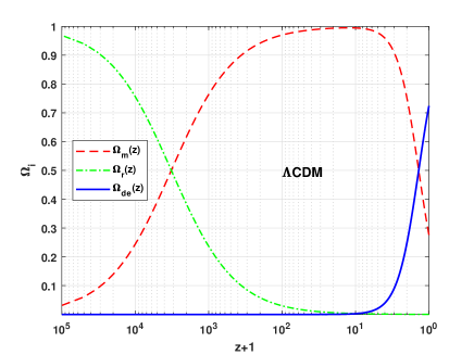
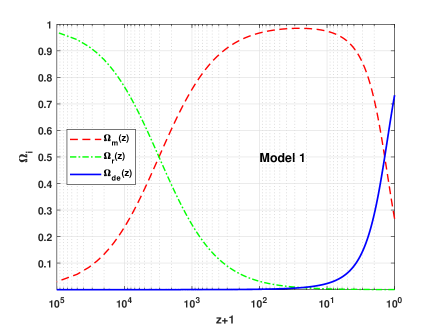
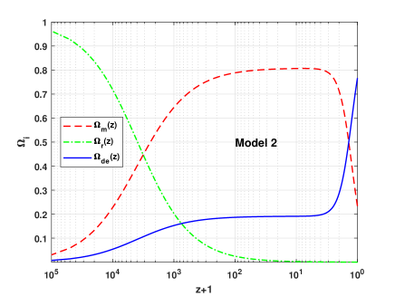
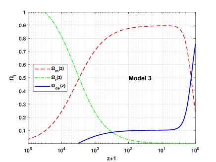
Figure 1: Redshift Evolution of radiation energy density $\Omega_{\rm r}(z)$, matter energy density $\Omega_{\rm m}(z)$ and DE density $\Omega_{\rm de}(z)$ for different cosmological models explored in this work. The style of the curves are presented in the inner panels.

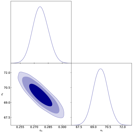
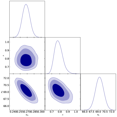
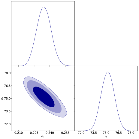
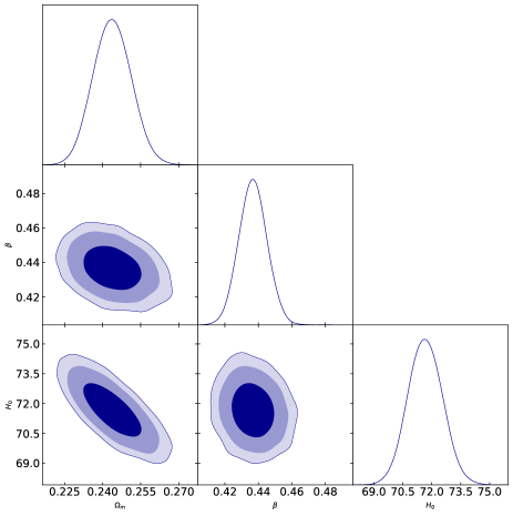
Figure 2: The $1\sigma$,$2\sigma$ and $3\sigma$ contours for various cosmological parameters using the background data. Different panels correspond to $\Lambda$CDM model (up-left), HDE model 1 (up-right), model 2 (bottom-left) and model 3 (bottom-right).

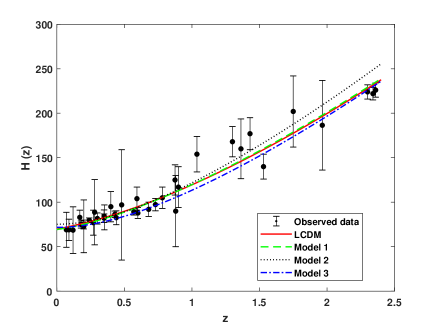
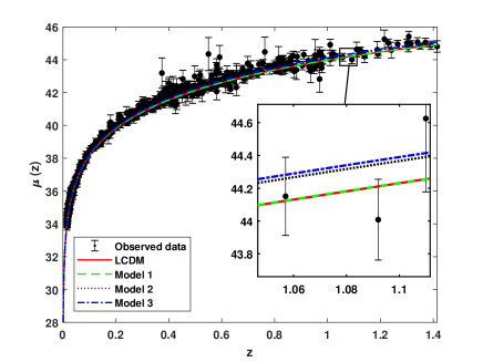
Figure 3: Comparison of the theoretical Hubble parameter (left panel) and the Supernova distance modulus (right panel) computed for different HDE and $\Lambda$CDM models respectively. On top of that we plot the corresponding data. The cosmological parameters are provided in Table (5). The style of the different lines are explained in the inner panel of the figure.

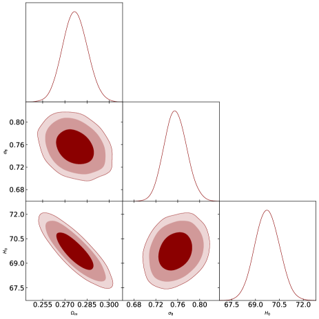
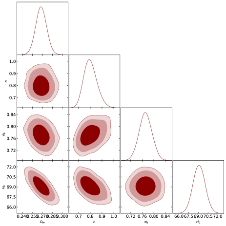
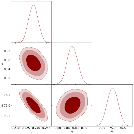
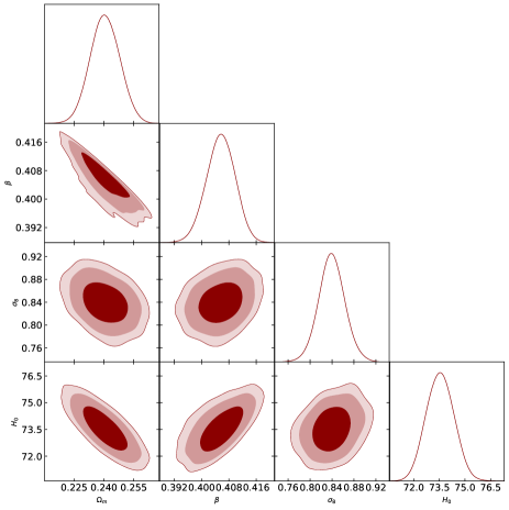
Figure 4: The $1\sigma$, $2\sigma$ and $3\sigma$ contours for various cosmological parameters. Here we used the combined background and growth rate data, assuming the HDE is homogeneous (see model 1: up-right, model 2: bottom-left and model 3: bottom right). The concordance $\Lambda$CDM is shown in up-left panel.

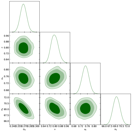
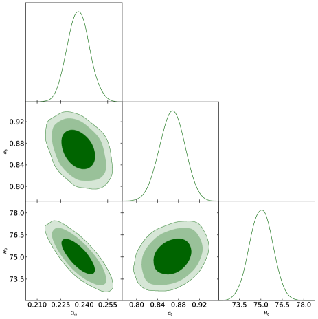
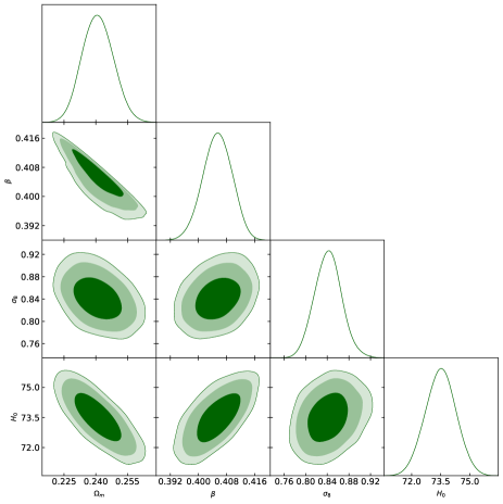
Figure 5: The $1\sigma$, $2\sigma$ and $3\sigma$ contours, considering that the HDE is allowed to cluster (see model 1: up-left panel, model 2: up-right panel and model 3: bottom).

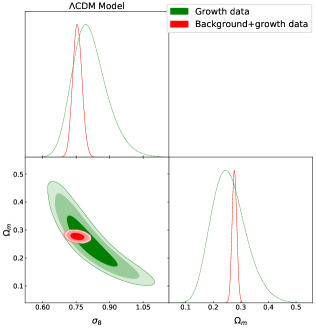
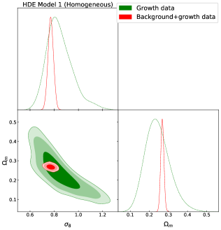
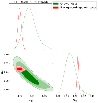
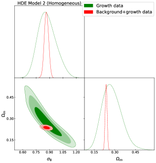
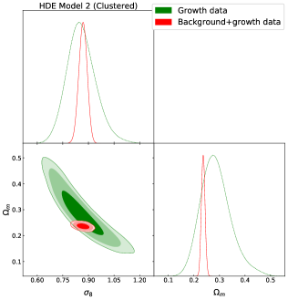
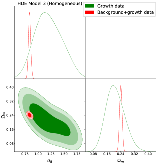
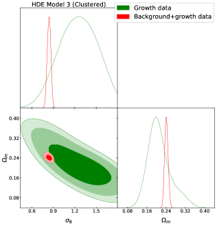
Figure 6: The $1\sigma$, $2\sigma$ and $3\sigma$ likelihood contours in $\sigma_{8}$- $\Omega_{\rm m}$ plane for different HDE models, including the concordance $\Lambda$CDM. The green contours correspond to the growth rate data, while the red contours obtained using the combination of expansion and growth data.

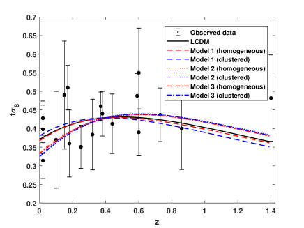
Figure 7: Comparison of the theoretical growth rate for different homogeneous HDE models. On top of that we plot the growth rate data ( see Table 3). For comparison we also include the predictions of the $\Lambda$CDM model. Line styles are explained in the inner plot of the figure.

2.2 Growth of perturbations

Here, we briefly review the basic features of the growth of linear matter perturbations in DE cosmologies. We focus our analysis at sub-horizon scales, where the results of Pseudo Newtonian dynamics are well consistent with those of General Relativity (GR) paradigm (see Abramo et al., 2007). In this context, two different scenarios have been studied in literature (Armendariz-Picon et al., 1999; Garriga & Mukhanov, 1999; Armendariz-Picon et al., 2000; Erickson et al., 2002; Bean & Doré, 2004; Hu & Scranton, 2004; Abramo et al., 2007, 2008; Bal, ; Abramo et al., 2009; Basilakos et al., 2009a; de Putter et al., 2010; Pace et al., 2010; Akhoury et al., 2011; Sapone & Majerotto, 2012; Pace et al., 2012; Batista & Pace, 2013; Dossett & Ishak, 2013; Batista, 2014; Basse et al., 2014; Pace et al., 2014b; Pace et al., 2014a; Pace et al., 2014c; Malekjani et al., 2015; Naderi et al., 2015; Mehrabi et al., 2015a, b; Mehrabi et al., 2015c; Nazari-Pooya et al., 2016; Malekjani et al., 2017). In the first scenario the DE component is homogeneous and only the corresponding non-relativistic matter is allowed to clump, while in the second scenario the whole system clusters (both matter and DE). For both treatments, we refer the reader to follow our previous articles (Mehrabi et al., 2015c; Malekjani et al., 2017) in which we have provided the basic differential equations which describe the situation at the perturbation level. Concerning the initial conditions, we use those provided by Batista & Pace (2013) (see also Mehrabi et al., 2015c; Malekjani et al., 2017). Here we study the growth of matter perturbations from the epoch of matter-radiation equality to the present time.

In the case of homogeneous DE models, DE affects the growth of matter perturbations via the Hubble parameter, while for clustered DE models, DE affects the growth of matter fluctuations through: (i) the modification of the Hubble rate and (ii) the direct influence of DE perturbations on the matter perturbations. Notice, that the DE fluctuations can grow in a similar way to matter perturbations. Of course, due to the impact of negative pressure the amplitude of DE perturbations is much smaller with respect to that of matter perturbations. Moreover, the influence of DE perturbations on the growth of matter fluctuations depends on the EoS parameter of DE. Indeed in the case of DE models with quintessence like EoS $-1<w_{\rm de}<-1/3$, DE perturbations causes the decrement of the amplitude of matter fluctuations (Abramo et al., 2007). On the other hand for phantom DE models ($w_{\rm de}<-1$), DE perturbations enhance the process of matter fluctuations growth (Abramo et al., 2007). In the following section, we consider both clustered and homogeneous HDE models and we compare the predicted growth rate of matter perturbations against the data.

Table 2: The $H(z)$ data. Notice that the values of $H(z)$ are in units [km/s/Mpc]

z	H(z)	References
$0.07$	$69.0^{+19.6}_{-19.6}$	Zhang et al. (2014a)
$0.09$	$69.0^{+12.0}_{-12.0}$	Jimenez et al. (2003)
$0.12$	$69.0^{+12.0}_{-12.0}$	Zhang et al. (2014a)
$0.17$	$83.0^{+8.0}_{-8.0}$	Simon et al. (2005)
$0.1791$	$75.0^{+4.0}_{-4.0}$	Moresco et al. (2012)
$0.1993$	$75.0^{+5.0}_{-5.0}$	Moresco et al. (2012)
$0.2$	$72.9^{+29.6}_{-29.6}$	Zhang et al. (2014a)
$0.27$	$77.0^{+14}_{-14}$	Simon et al. (2005)
$0.28$	$88.8^{+36.6}_{-36.6}$	Zhang et al. (2014a)
$0.3519$	$83.0^{+14.0}_{-14.0}$	Moresco et al. (2012)
$0.3802$	$83.0^{+13.5}_{-13.5}$	Moresco et al. (2016)
$0.4$	$95.0^{+17.0}_{-17.0}$	Simon et al. (2005)
$0.4004$	$77.0^{+10.2}_{-10.2}$	Moresco et al. (2016)
$0.4247$	$87.1^{+11.2}_{-11.2}$	Moresco et al. (2016)
$0.4497$	$92.8^{+12.9}_{-12.9}$	Moresco et al. (2016)
$0.4783$	$80.9^{+9.0}_{-9.0}$	Moresco et al. (2016)
$0.48$	$97.0^{+62.0}_{-62.0}$	Stern et al. (2010)
$0.5929$	$104.0^{+13.0}_{-13.0}$	Moresco et al. (2012)
$0.6797$	$92.0^{+8.0}_{-8.0}$	Moresco et al. (2012)
$0.7812$	$105.0^{+12.0}_{-12.0}$	Moresco et al. (2012)
$0.8754$	$125.0^{+17.0}_{-17.0}$	Moresco et al. (2012)
$0.88$	$90.0^{+40.0}_{-40.0}$	Stern et al. (2010)
$0.90$	$117.0^{+23.0}_{-23.0}$	Simon et al. (2005)
$1.037$	$154.0^{+20.0}_{-20.0}$	Moresco et al. (2012)
$1.3$	$168.0^{+17.0}_{-17.0}$	Moresco et al. (2012)
$1.363$	$160.0^{+33.0}_{-33.0}$	Moresco (2015)
$1.43$	$177.0^{+18.0}_{-18.0}$	Simon et al. (2005)
$1.53$	$140.0^{+14.0}_{-14.0}$	Simon et al. (2005)
$1.75$	$202.0^{+40.0}_{-40.0}$	Simon et al. (2005)
$1.965$	$186.0^{+50.4}_{-50.4}$	Moresco (2015)

Table 3: The growth rate $f(z)\sigma_{8}(z)$ data.

$z$	$f(z)\sigma_{8}(z)$	References
$0.02$	$0.428^{+0.0465}_{-0.0465}$	Huterer et al. (2017)
$0.02$	$0.398^{+0.065}_{-0.065}$	Hudson & Turnbull (2013),Turnbull et al. (2012)
$0.02$	$0.314^{+0.048}_{-0.048}$	Hudson & Turnbull (2013),Davis et al. (2011)
$0.10$	$0.370^{+0.130}_{-0.130}$	Feix et al. (2015)
$0.15$	$0.490^{+0.145}_{-0.145}$	Howlett et al. (2015)
$0.17$	$0.510^{+0.060}_{-0.060}$	Song & Percival (2009)
$0.18$	$0.360^{+0.090}_{-0.090}$	Blake et al. (2013)
$0.38$	$0.440^{+0.060}_{-0.060}$	Blake et al. (2013)
$0.25$	$0.3512^{+0.0583}_{-0.0583}$	Samushia et al. (2012)
$0.37$	$0.4602^{+0.0378}_{-0.0378}$	Samushia et al. (2012)
$0.32$	$0.384^{+0.095}_{-0.095}$	Sanchez et al. (2014)
$0.59$	$0.488^{+0.060}_{-0.060}$	Chuang et al. (2016)
$0.44$	$0.413^{+0.080}_{-0.080}$	Blake et al. (2012)
$0.60$	$0.390^{+0.063}_{-0.063}$	Blake et al. (2012)
$0.73$	$0.437^{+0.072}_{-0.072}$	Blake et al. (2012)
$0.60$	$0.550^{+0.120}_{-0.120}$	Pezzotta et al. (2017)
$0.86$	$0.400^{+0.110}_{-0.110}$	Pezzotta et al. (2017)
$1.40$	$0.482^{+0.116}_{-0.116}$	Okumura et al. (2016)

Table 4: Results of statistical likelihood analysis using different sets of background data for various HDE models and standard $\Lambda$CDM universe.

Model	Model (1)	Model (2)	Model (3)	$\Lambda$CDM
$k$	4	3	4	3
$\chi^{2}_{\rm min}$(total)	591.28	728.52	657.56	587.64
$\chi^{2}_{\rm best}$(SNIa)	562.43	600.53	609.09	562.23
$\chi^{2}_{\rm best}$(Hubble)	22.04	48.17	28.85	20.63
$\chi^{2}_{\rm best}$(BBN)	0.18	3.84	0.68	0.02
$\chi^{2}_{\rm best}$(CMB: WMAP data)	2.25	50.98	6.66	0.59
$\chi^{2}_{\rm best}$(BAO)	4.37	25.00	12.29	4.17
AIC	599.28	734.52	665.56	593.64
BIC	616.04	747.84	683.32	606.96

Table 5: Best-fit parameters for the various HDE models using the cosmological data at background level.

Model	Model(1)	Model(2)	Model(3)	$\Lambda$CDM
$\Omega_{\rm m}$	$0.2677_{-0.0082,-0.016,-0.021}^{+0.0082,+0.016,+0.022}$	$\Omega_{m}=0.2344_{-0.0070,-0.013,-0.017}^{+0.0070,+0.014,+0.019}$	$0.2438_{-0.0075,-0.014,-0.019}^{+0.0075,+0.015,+0.020}$	$0.2767_{-0.0083,-0.016,-0.021}^{+0.0083,+0.017,+0.022}$
$H_{0}$	$69.29_{-0.92,-1.80,-2.40}^{+0.92,+1.80,+2.30}$	$75.20_{-0.79,-1.50,-2.10}^{+0.79,+1.50,+2.00}$	$71.66_{-0.90,-1.70,-2.30}^{+0.90,+1.80,2.40}$	$69.74_{-0.77,+1.50,+1.90}^{+0.77,-1.50,-1.90}$
$n$	$0.785^{+0.042,+0.10,+0.15}_{-0.056,-0.094,-0.11}$	–	–	–
$\beta$	–	–	$0.4369_{-0.0090,-0.016,-0.022}^{+0.0090,+0.017,+0.023}$	–
$w_{\rm de}(z=0)$	-1.10	-1.29	-1.32	-1.00
$\Omega_{\rm de}(z=0)$	0.71372	0.77314	0.75447	0.72627

Table 6: Numerical results for different homogeneous HDE models (part A) and clustered HDE models (part B) using the growth rate data. The results for concordance $\Lambda$CDM universe are shown for comparison.

Part (A)	Model 1 (homogeneous)	Model 2 (homogeneous)	Model 3 (homogeneous)	$\Lambda$CDM
$\chi^{2}_{\rm min}(gr)$	11.2	11.9	11.1	11.5
AIC (BIC)	19.2 (19.6)	17.9 (18.8)	19.1 (19.5)	17.5 (18.4)
$\Omega_{\rm m}$	$0.242_{-0.070,-0.12,-0.14}^{+0.055,+0.13,+0.20}$	$0.277_{-0.077,-0.013,-0.016}^{+0.061,+0.14,+0.20}$	$0.216_{-0.083,-0.12,-0.14}^{+0.052,+0.14,+0.22}$	$0.257_{-0.07,-0.12,-0.13}^{+0.052,+0.13,+0.18}$
$\sigma_{8}$	$0.844_{-0.12,-0.20,-0.22}^{+0.080,+0.23,+0.35}$	$0.872_{-0.11,-0.18,-0.20}^{+0.089,+0.21,+0.26}$	$1.27_{-0.48,-0.54,-0.57}^{+0.24,+0.78,+0.87}$	$0.813_{-0.087,-0.14,-0.16}^{+0.061,+0.16,+0.24}$
Part (B)	Model 1 (clustered)	Model 2 (clustered)	Model 3 (clustered)
$\chi^{2}_{\rm min}(gr)$	11.2	12.0	11.1
AIC (BIC)	19.2(19.6)	18.0 (18.9)	19.1 (19.6)
$\Omega_{\rm m}$	$0.198^{+0.046,+0.10,+0.15}_{-0.054,-0.096,-0.12}$	$0.285^{+0.048,+0.12,+0.18}_{-0.065,-0.11,-0.13}$	$0.212^{+0.034,+0.12,+0.15}_{-0.056-0.84,-0.094}$
$\sigma_{8}$	$0.873^{+0.064,+0.17,+0.22}_{-0.085,-0.15,-0.17}$	$0.858^{+0.074,+0.18,+0.26}_{-0.089,-0.16,-0.19}$	$1.25^{+0.32,+0.52,+0.64}_{-0.28,-0.51,-0.63}$

Table 7: Results of statistical likelihood analysis using different sets of background data combined with growth rate data $f(z)\sigma_{8}(z)$ for various homogeneous and clustered HDE models. The standard $\Lambda$CDM universe is shown for comparison. Values inside the parenthesis belong to clustered HDE models.

Model	Model 1	Model 2	Model 3	$\Lambda$CDM
$k$	5	4	5	4
$\chi^{2}_{\rm min}${total}	599.61 (599.34)	739.90 (740.75)	687.15 (688.20)	596.08
AIC {total}	609.61 (609.34)	747.90 (748.75)	697.15 (798.20)	604.08
BIC {total}	630.96 (631.69)	765.78 (766.63)	719.50 (720.55)	621.96

Table 8: Best-fit parameters for the various homogeneous HDE models and concordance $\Lambda$CDM universe using the combined background and growth rate data.

Model	Model(1)	Model(2)	Model(3)	$\Lambda$CDM
$\Omega_{\rm m}$	$0.2680_{-0.0084,-0.016,-0.022}^{+0.0084,+0.017,+0.023}$	$0.2361_{-0.0069,-0.013,-0.017}^{+0.0069,+0.014,+0.018}$	$0.2405_{-0.0073,-0.014,-0.019}^{+0.0073,+0.014,+0.019}$	$0.2769_{-0.0084,-0.016,-0.022}^{+0.0084,+0.017,+0.022}$
$H_{0}$	$69.12_{-0.94,-1.8,-2.4}^{+0.94,+1.9,+2.4}$	$75.05_{-0.78,-1.5,-1.9}^{+0.78,+1.5,+1.9}$	$73.56_{-0.79,-1.5,-1.9}^{+0.79,+1.5,+2.1}$	$69.74_{-0.77,-1.5,-2.0}^{+0.77,+1.5,+2.0}$
$\sigma_{8}$	$0.771_{-0.023,-0.044,-0.057}^{+0.023,+0.044,+0.058}$	$0.866_{-0.024,-0.047,-0.063}^{+0.024,+0.047,+0.061}$	$0.840_{-0.025,-0.050,-0.069}^{+0.025,+0.047,+0.066}$	$0.756_{-0.020,-0.039,-0.050}^{+0.020,+0.041,+0.054}$
$n$	$0.801^{+0.049,+0.11,+0.16}_{-0.061,-0.10,-0.12}$	–	–	–
$\beta$	–	–	$0.4057_{-0.0041,-0.0080,-0.010}^{+0.0041,+0.0080,+0.010}$	–

Table 9: Best-fit parameters for the various clustered HDE models using the cosmological data for background+growth analysis.

Model	Model(1)	Model(2)	Model(3)	$\Lambda$CDM
$\Omega_{\rm m}$	$0.2673_{-0.0083,-0.016,-0.021}^{+0.0083,+0.017,+0.023}$	$0.2364_{-0.0071,-0.013,-0.017}^{+0.0071,+0.014,+0.019}$	$0.2413^{+0.0067,+0.015,+0.019}_{-0.0078,-0.014,-0.018}$	$-$
$H_{0}$	$69.21_{-0.91,-1.7,-2.3}^{0.91,+1.8,+2.4}$	$75.03_{-0.80,-1.6,-2.0}^{+0.80,+1.6,+2.1}$	$73.48_{-0.79,-1.6,-2.0}^{+0.79,+1.5,+2.0}$	$-$
$\sigma_{8}$	$0.749_{-0.021,-0.041,-0.053}^{+0.021,+0.041,+0.057}$	$0.868_{-0.024,-0.048,-0.063}^{+0.024,+0.046,+0.059}$	$0.839_{-0.025,-0.049,-0.060}^{+0.025,+0.048,+0.062}$	$-$
$n$	$0.797^{+0.047,+0.10,+0.14}_{-0.054,-0.096,-0.12}$	–	–	–
$\beta$	–	–	$0.4052_{-0.0041,-0.0084,-0.010}^{+0.0041,+0.0075,+0.0097}$	–

3 HDE models against observational data

In this section, we first implement a likelihood statistical analysis in order to place constraints on the free parameters of the current HDE models using solely expansion data. Second, utilizing the growth rate data we check the performance of the current HDE models at the perturbation level. Finally, based on the Akaike and Bayesian information criteria we study the ability of the combined (expansion+growth) data in constraining the cosmological parameters of HDE models and we statistically compare them against the $\Lambda$CDM model.

3.1 Expansion data

Let us start with a brief description of the expansion data. Specifically, the latest expansion data used in our analysis are SnIa (Suzuki et al., 2012), BAO (Beutler et al., 2011; Padmanabhan et al., 2012; Anderson et al., 2013; Blake et al., 2011b), CMB (Hinshaw et al., 2013), BBN (Serra et al., 2009; Burles et al., 2001), Hubble data (Moresco et al., 2012; Gaztanaga et al., 2009; Blake et al., 2012; Anderson et al., 2014). In order to trace the Hubble relation we use 580 SnIa provided by the Union2.1 sample (Suzuki et al., 2012) and 37 $H(z)$ measurements from the Hubble data (see Table 2). Moreover, we include in the analysis the BAO data based on 6 distinct measurements of the baryon acoustic scale (see Tab.1 of Mehrabi et al., 2015b, and references therein). and the WMAP data concerning the position of CMB acoustic peak as described in Shafer & Huterer (2014) (see also Mehrabi et al., 2015b). Lastly, we utilize the Big Bang Nucleosynthesis (BBN) point which constrains the value of $\Omega_{\rm b0}$ (Serra et al., 2009). For more details regarding the MCMC technique used, we refer the reader to Mehrabi et al. (2015b) (see also Basilakos et al., 2009b; Hinshaw et al., 2013; Mehrabi et al., 2015c, 2017; Malekjani et al., 2017).

Following standard lines the overall likelihood function is written as the product of the individual likelihoods:

$${\cal L}_{\rm tot}({\bf p})={\cal L}_{\rm sn}\times{\cal L}_{\rm bao}\times{\cal L}_{\rm cmb}\times{\cal L}_{\rm h}\times{\cal L}_{\rm bbn}\;,$$ (22)

and thus the total chi-square $\chi^{2}_{\rm tot}$ is given by:

$$\chi^{2}_{\rm tot}({\bf p})=\chi^{2}_{\rm sn}+\chi^{2}_{\rm bao}+\chi^{2}_{\rm cmb}+\chi^{2}_{\rm h}+\chi^{2}_{\rm bbn}\;,$$ (23)

where the statistical vector ${\bf p}$ includes the free parameters that we want to constrain. In our case this vector becomes: (a) ${\bf p}=\{\Omega_{\rm DM0},\Omega_{\rm b0},H_{0},n\}$ for model (1), (b) ${\bf p}=\{\Omega_{\rm DM0},\Omega_{\rm b0},H_{0}\}$ for model (2) and (c) ${\bf p}=\{\Omega_{\rm DM0},\Omega_{\rm b0},H_{0},\beta\}$ in the case of model (3). Notice that regarding the value of $\Omega_{\rm r0}$ we have set it to $\Omega_{\rm r0}=2.469\times 10^{-5}h^{-2}(1.6903)$ where $h=H_{0}/100$ (Hinshaw et al., 2013).

Furthermore, in order to identify the statistical significance of our results we utilize the well known AIC and BIC criteria. Assuming Gaussian errors the AIC (Akaike, 1974) and BIC (Schwarz, 1978) estimators are given by

$${\rm AIC}=-2\ln{\cal L}_{\rm max}+2k+\frac{2k(k+1)}{N-k-1}\;,$$ (24)

$${\rm BIC}=-2\ln{\cal L}_{\rm max}+k\ln{N}\;,$$ (25)

where $N$ is the total number of data and $k$ is the number of free parameters (see also Liddle, 2007). Our main statistical results are shown in Tables (4) and (5), in which we provide the goodness of fit statistics ($\chi_{\rm min}^{2}$, AIC, BIC) and the fitted cosmological parameters with the corresponding $\sigma$ uncertainties, for three different HDE models (see section 2.1). For comparison we also present the results of the concordance $\Lambda$CDM model. From the viewpoint of AIC analysis, it is clear that a smaller value of AIC implies a better model-data fit. Also, in order to test, the statistical performance of the different models in reproducing the observational data, we need to utilize the model pair difference $\Delta{\rm AIC}={\rm AIC}_{\rm model}-{\rm AIC}_{\rm min}$. It has been found that the restriction $4<\Delta{\rm AIC}<7$ suggests a positive evidence against the model with higher value of ${\rm AIC}_{\rm model}$ (Anderson, 2002, 2004), while the inequality $\Delta{\rm AIC}\geq 10$ suggests a strong such evidence. In this framework, for $\Delta{\rm AIC}\leq 2$ we have an indication of consistency between the two comparison models. Concerning the BIC criterion, the model with the lowest BIC value is the best model. The model pair difference $\Delta{\rm BIC}={\rm BIC}_{\rm model}-{\rm BIC}_{\rm min}$ provides the following situations: (i) $\Delta{\rm BIC}\leq 2$ indicates that the comparison model is consistent with the best model, (ii) the inequality $2<\Delta{\rm BIC}<6$ points positive evidence against the comparison model, while for $\Delta{\rm BIC}>10$ such evidence becomes strong.

As expected, after considering the aforementioned arguments we find that the best model is the $\Lambda$CDM model and thus ${\rm AIC}_{\rm min}\equiv{\rm AIC}_{\Lambda}$. ${\rm BIC}_{\rm min}\equiv{\rm BIC}_{\Lambda}$. We also find a strong evidence against HDE models (2) and (3), since the corresponding pair difference is $\Delta{\rm AIC}>10$ and $\Delta{\rm BIC}>10$. Moreover, we observe a relative weak evidence against the HDE model (1), $\Delta{\rm AIC}\simeq 5.6$ and $\Delta{\rm BIC}\simeq 9$. It is interesting to mention that our results are in agreement with the theoretical results of (Basilakos & Sola, 2014) (see also Xu & Zhang, 2016). Basilakos & Sola (2014) who proved that the HDE models (2) and (3) for which both kind of Hubble terms $H$ and ${\dot{H}}$ appear in the effective dark energy $\rho_{\rm de}$ are not viable neither at the background nor at the cosmic perturbations level. But let us try to understand the reason that HDE models (2) and (3) are disfavored by the expansion data.

Using the best fit values of Table (5), we show in Fig.(1) the evolution of energy densities, namely radiation $\Omega_{\rm r}$, pressureless matter $\Omega_{\rm m}$ and dark energy $\Omega_{\rm de}$ for the current HDE models. As far as the dark energy density is concerned we utilize the relations (11, 14 & • ‣ 2.1) that correspond to HDE model (1), model (2) and model (3), respectively. On top of that we also plot the evolution of energy densities of the $\Lambda$CDM model for comparison. As expected in the case of $\Lambda$CDM model, we see that in the early matter dominated era the DE density is negligible with respect to the other components. However, for HDE models (2) & (3) we find that the DE component affects the cosmic expansion at early times. For example, prior to $z\simeq 1100$ we find that $\Omega_{d}$ tends to 0.18 and 0.06 for HDE models (2) and (3) respectively. The latter has an impact on the cosmic expansion and eventually it leads to the aforementioned statistical result, namely HDE models (2) and (3) are ruled out by the expansion data. Therefore, for the rest of the current sub-section we focus on HDE model (1). In this case we obtain $n=0.785^{+0.042,+0.10,+0.15}_{-0.056,-0.094,-0.11}$ which implies that the present value of the EoS parameter of this model can cross the phantom line $w(z=0)\simeq-1.06$. Notice, that similar results can be found in previous works (Shen et al., 2005; Kao et al., 2005; Yi & Zhang, 2007; Zhang et al., 2012; Huang & Gong, 2004; Zhang & Wu, 2005; Chang et al., 2006; Zhang & Wu, 2007; Ma et al., 2009; Xu, 2012, 2013; Li et al., 2013; Mehrabi et al., 2015c). In Fig. (2) we plot the $1\sigma$, $2\sigma$ and $3\sigma$ confidence regions in various planes for HDE and $\Lambda$CDM models respectively. The negative correlation between the Hubble constant $H_{0}$ and the matter energy density $\Omega_{\rm m}$ (baryons+dark matter) implies that if we increase the amount of the present energy density of matter then the Hubble constant decreases. In the case of HDE model (1), the negative correlation between model parameter $n$ and $H_{0}$ is also present. Now, utilizing the cosmological parameters of Table (5) we plot the Hubble parameter $H(z)$ (left panel) and the distance modulus $\mu(z)=m-M$ of SNIa (right panel) as a function of redshift in Fig.(3). The predictions of the concordance $\Lambda$CDM are also shown for comparison (solid curve). From both diagrams, we observe that HDE model (1) is relatively close to that of the standard $\Lambda$CDM model.

3.2 Growth rate data

Now we focus our analysis at the perturbation level, namely we use only the growth rate data. Since the growth data are given in terms of $f(z)\sigma_{8}(z)$ the first step is to theoretically calculate the latter quantity for the HDE models. Notice, that $f=d\ln{\delta_{m}}/d\ln{a}$ is the growth rate of matter perturbations and $\sigma_{8}(z)=D(z)\sigma_{8}(z=0)$ is the r.m.s. mass fluctuations within $R=8h^{-1}$Mpc at redshift $z$, where $D(z)=\delta_{\rm m}(z)/\delta_{\rm m}(z=0)$ is the linear growth factor. Using 18 robust and independent $f\sigma_{8}$ measurements ( see Table 3), we perform a likelihood analysis involving the growth data. Note, that even though the number of growth data has increased greatly since 2010, the data are not independent from each other and thus they should not be used all together at the same time ( for mode details see Nesseris et al., 2017). For the growth rate data the corresponding likelihood function ${\cal L}_{\rm gr}({\bf p})$ is written as

$$\chi^{2}_{\rm gr}({\bf p})=\sum_{i}\frac{\left([f(z_{i},{\bf p})\sigma_{8}(z_{i},{\bf p})]_{theor}-[f(z_{i})\sigma_{8}(z_{i})]_{obs}\right)^{2}}{\sigma_{\rm i}^{2}}\;,$$ (26)

where the subscript "theor" indicates the theoretical value, "obs" stands for observational value and $\sigma_{i}$ is the uncertainty of the growth data. Here the statistical vector ${\bf p}$ includes an additional free parameter, namely $\sigma_{8}$ which is the present value of the rms fluctuations. The statistical results of this section are summarized in Tab.(6). Notice, that this table does not include the Hubble constant, since $H_{0}$ enters only in the radiation density parameter $\Omega_{\rm r0}=2.469\times 10^{-5}h^{-2}(1.6903)$ (Hinshaw et al., 2013), hence it is not really affect the cosmic expansion at relatively low redshifts. Also, in Fig. 6 (green contours) we visualize $1\sigma$, $2\sigma$ and $3\sigma$ confidence levels in the $\sigma_{8}-\Omega_{\rm m}$ plane. It becomes clear that the growth data can not place strong constraints on the cosmological models. Moreover, AIC and BIC tests suggest that $\Lambda$CDM is the best model. However, we find that using the growth data alone the corresponding pair differences of all HDE models are: $\Delta{\rm AIC}\leq 2$ and $\Delta{\rm BIC}\leq 3$. The latter implies that the current HDE models are statistically equivalent with that of $\Lambda$CDM at the perturbation level, regards-less the status of the DE.

3.3 Combined expansion and growth data

In this section using the MCMC algorithm we implement an overall statistical analysis combining the expansion and the growth rate data. The statistical results concerning the clustered and homogeneous HDE models are presented in Tables (8 & 9). Notice, that in the case of $\Lambda$CDM model DE does not cluster. Comparing the expansion and the growth rate data we find that the best fit parameters are roughly the same (within $1\sigma$ errors) to those provided by the background data. In Figs.(4 & 5), we present the $1\sigma$, $2\sigma$ and $3\sigma$ confidence contours for different types of DE, namely homogeneous and clustered. Based on the joint (background+growth) analysis the AIC and BIC tests show that the $\Lambda$CDM model is the best model, while they indicate that the cosmological data disfavor HDE models (2 & 3). Moreover, AIC suggests weak evidence against HDE model (1) ($\Delta{\rm AIC}\simeq 5.5$), while BIC indicates strong such evidence ($\Delta{\rm BIC}\simeq 8$). Therefore, based on the latter comparison we cannot reject this model. In Fig.(6), we plot the likelihood contours (red plots) in the $\sigma_{8}-\Omega_{\rm m}$ plane. Evidently, the combined analysis of expansion and growth rate data reduces significantly the parameter space, providing tight constraints on the cosmological parameters. Finally, with the aid of the best fit solutions provided in Tables (8 & 9), we plot in Fig.(7) the evolution of $f(z)\sigma_{(}z)$ for homogeneous and clustered HDE models respectively. Notice that the solid points correspond to the growth data. As we have already described above the explored cosmological models are in agreement with the growth rate data.

4 conclusion

In this work we compared the most popular Holographic dark energy models with the latest observational data. These HDE models were constructed on the basis of the event horizon IR cutoff (model 1), the Ricci scale IR cutoff (model 2) and the Granda & Oliveros (GO) IR cutoff (model 3), respectively. Initially, we implemented a standard likelihood analysis using the latest expansion data (SNIa, BBN, BAO, CMB and $H(z)$) and we placed constraints on the free parameters of the HDE models. Combining the well known Akaike and Bayesian information criteria we found that the data disfavor the HDE models (2) and (3). We also found that the HDE model (1) cannot be rejected by the geometrical data. The latter result can be understood in the context of early dark energy, namely unlike HDE model (1), the rest of the HDE models predict a small but non-negligible amount of DE at early enough times. As expected, after considering the aforementioned statistical tests we verified that the best model is the $\Lambda$CDM model. Moreover, we found that the latter results remains unaltered if we combine the growth rate data with those of the expansion data. Finally, focusing at the perturbation level, namely using only the growth rate data we found that the current HDE models are in agreement with the data, regard-less the status of the DE component (homogeneous or clustered). However, we found that the growth rate data alone can not be used toward constraining the HDE models.

References

- Abramo et al. (2007) Abramo L. R., Batista R. C., Liberato L., Rosenfeld R., 2007, JCAP, 11, 12
- Abramo et al. (2008) Abramo L. R., Batista R. C., Liberato L., Rosenfeld R., 2008, Phys. Rev. D, 77, 067301
- Abramo et al. (2009) Abramo L. R., Batista R. C., Liberato L., Rosenfeld R., 2009, Phys. Rev., D79, 023516
- Akaike (1974) Akaike H., 1974, ITAC, 19, 716
- Akhoury et al. (2011) Akhoury R., Garfinkle D., Saotome R., 2011, JHEP, 04, 096
- Anderson (2002) Anderson K. . P. B. . D. R., 2002, Model selection and multimodel inference: a practical information-theoretic approach, 2nd edn. Springer, New York
- Anderson (2004) Anderson K. . P. B. . D. R., 2004, Sociological Methods & Research, 33, 261
- Anderson et al. (2013) Anderson L., et al., 2013, Mon. Not. Roy. Astron. Soc., 427, 3435
- Anderson et al. (2014) Anderson L., et al., 2014, Mon. Not. Roy. Astron. Soc., 441, 24
- Armendariz-Picon et al. (1999) Armendariz-Picon C., Damour T., Mukhanov V. F., 1999, Phys. Lett., B458, 209
- Armendariz-Picon et al. (2000) Armendariz-Picon C., Mukhanov V. F., Steinhardt P. J., 2000, Phys. Rev. Lett., 85, 4438
- (12)
- Bamba et al. (2012) Bamba K., Myrzakulov R., Nojiri S., Odintsov S. D., 2012, Phys. Rev., D85, 104036
- Basilakos (2015) Basilakos S., 2015, Mon. Not. Roy. Astron. Soc., 449, 2151
- Basilakos (2016) Basilakos S., 2016, Phys. Rev., D93, 083007
- Basilakos & Pouri (2012) Basilakos S., Pouri A., 2012, MNRAS, 423, 3761
- Basilakos & Sola (2014) Basilakos S., Sola J., 2014, Phys. Rev., D90, 023008
- Basilakos et al. (2009a) Basilakos S., Bueno Sanchez J. C., Perivolaropoulos L., 2009a, Phys. Rev., D80, 043530
- Basilakos et al. (2009b) Basilakos S., Plionis M., Sola J., 2009b, Phys. Rev., D80, 083511
- Basilakos et al. (2010) Basilakos S., Plionis M., Lima J. A. S., 2010, Phys. Rev., D82, 083517
- Basse et al. (2014) Basse T., Bjaelde O. E., Hamann J., Hannestad S., Wong Y. Y. Y., 2014, JCAP, 1405, 021
- Batista (2014) Batista R. C., 2014, Phys. Rev., D89, 123508
- Batista & Pace (2013) Batista R. C., Pace F., 2013, JCAP, 1306, 044
- Bean & Doré (2004) Bean R., Doré O., 2004, Phys. Rev. D, 69, 083503
- Beutler et al. (2011) Beutler F., Blake C., Colless M., Jones D. H., Staveley-Smith L., et al., 2011, MNRAS, 416, 3017
- Blake et al. (2011a) Blake C., et al., 2011a, Mon. Not. Roy. Astron. Soc., 415, 2876
- Blake et al. (2011b) Blake C., Kazin E., Beutler F., Davis T., Parkinson D., et al., 2011b, MNRAS, 418, 1707
- Blake et al. (2012) Blake C., et al., 2012, Mon. Not. Roy. Astron. Soc., 425, 405
- Blake et al. (2013) Blake C., et al., 2013, Mon. Not. Roy. Astron. Soc., 436, 3089
- Bonilla Rivera & Farieta (2016) Bonilla Rivera A., Farieta J. G., 2016
- Burles et al. (2001) Burles S., Nollett K. M., Turner M. S., 2001, ApJ, 552, L1
- Carroll (2001) Carroll S. M., 2001, Living Reviews in Relativity, 380, 1
- Cataldo et al. (2001) Cataldo M., Cruz N., del Campo S., Lepe S., 2001, Physics Letters B, 509, 138
- Chang et al. (2006) Chang Z., Wu F.-Q., Zhang X., 2006, Phys. Lett., B633, 14
- Chuang et al. (2013) Chuang C.-H., et al., 2013, Mon. Not. Roy. Astron. Soc., 433, 3559
- Chuang et al. (2016) Chuang C.-H., et al., 2016, Mon. Not. Roy. Astron. Soc., 461, 3781
- Cohen et al. (1999) Cohen A. G., Kaplan D. B., Nelson A. E., 1999, Physical Review Letters, 82, 4971
- Contreras et al. (2013) Contreras C., et al., 2013, ] 10.1093/mnras/sts608
- Cooray et al. (2004) Cooray A., Huterer D., Baumann D., 2004, Phys. Rev., D69, 027301
- Copeland et al. (2006) Copeland E. J., Sami M., Tsujikawa S., 2006, IJMP, D15, 1753
- Corasaniti et al. (2005) Corasaniti P.-S., Giannantonio T., Melchiorri A., 2005, Phys. Rev., D71, 123521
- Davis et al. (2011) Davis M., Nusser A., Masters K., Springob C., Huchra J. P., Lemson G., 2011, Mon. Not. Roy. Astron. Soc., 413, 2906
- Dossett & Ishak (2013) Dossett J., Ishak M., 2013, Phys. Rev., D88, 103008
- Easson et al. (2011) Easson D. A., Frampton P. H., Smoot G. F., 2011, Phys. Lett., B696, 273
- Easson et al. (2012) Easson D. A., Frampton P. H., Smoot G. F., 2012, Int. J. Mod. Phys., A27, 1250066
- Erickson et al. (2002) Erickson J. K., Caldwell R., Steinhardt P. J., Armendariz-Picon C., Mukhanov V. F., 2002, Phys. Rev. Lett., 88, 121301
- Fay (2016) Fay S., 2016, ] 10.1093/mnras/stw1087
- Feix et al. (2015) Feix M., Nusser A., Branchini E., 2015, Phys. Rev. Lett., 115, 011301
- Frieman et al. (2008) Frieman J., Turner M., Huterer D., 2008, Ann. Rev. Astron. Astrophys., 46, 385
- Gannouji et al. (2010) Gannouji R., Moraes B., Mota D. F., Polarski D., Tsujikawa S., Winther H. A., 2010, Phys. Rev., D82, 124006
- Gao et al. (2009) Gao C., Chen X., Shen Y.-G., 2009, Phys. Rev., D79, 043511
- Garriga & Mukhanov (1999) Garriga J., Mukhanov V. F., 1999, Phys. Lett., B458, 219
- Gaztanaga et al. (2009) Gaztanaga E., Cabre A., Hui L., 2009, Mon. Not. Roy. Astron. Soc., 399, 1663
- Granda & Oliveros (2008) Granda L. N., Oliveros A., 2008, Phys. Lett., B669, 275
- Hinshaw et al. (2013) Hinshaw G., et al., 2013, Astrophys. J. Suppl., 208, 19
- Hořava & Minic (2000) Hořava P., Minic D., 2000, Physical Review Letters, 85, 1610
- Howlett et al. (2015) Howlett C., Ross A., Samushia L., Percival W., Manera M., 2015, Mon. Not. Roy. Astron. Soc., 449, 848
- Hsu (2004) Hsu S. D. H., 2004, Physical Letters B, 594, 13
- Hu & Scranton (2004) Hu W., Scranton R., 2004, Phys. Rev. D, 70, 123002
- Huang & Gong (2004) Huang Q.-G., Gong Y.-G., 2004, JCAP, 0408, 006
- Hudson & Turnbull (2013) Hudson M. J., Turnbull S. J., 2013, Astrophys. J., 751, L30
- Huterer et al. (2017) Huterer D., Shafer D., Scolnic D., Schmidt F., 2017, JCAP, 1705, 015
- Jimenez et al. (2003) Jimenez R., Verde L., Treu T., Stern D., 2003, Astrophys. J., 593, 622
- Kao et al. (2005) Kao H.-C., Lee W.-L., Lin F.-L., 2005, Phys. Rev., D71, 123518
- Koivisto & Mota (2007) Koivisto T., Mota D. F., 2007, Phys. Lett., B644, 104
- Li (2004a) Li M., 2004a, Physics Letters B, 603, 1
- Li (2004b) Li M., 2004b, Phys. Lett., B603, 1
- Li et al. (2011) Li B., Sotiriou T. P., Barrow J. D., 2011, Phys. Rev., D83, 104017
- Li et al. (2013) Li M., Li X.-D., Ma Y.-Z., Zhang X., Zhang Z., 2013, JCAP, 1309, 021
- Li et al. (2014) Li J., Yang R., Chen B., 2014, JCAP, 1412, 043
- Liddle (2007) Liddle A. R., 2007, Mon. Not. Roy. Astron. Soc., 377, L74
- Llinares & Mota (2013) Llinares C., Mota D., 2013, Phys. Rev. Lett., 110, 161101
- Llinares et al. (2014) Llinares C., Mota D. F., Winther H. A., 2014, Astron. Astrophys., 562, A78
- Ma et al. (2009) Ma Y. Z., Gong Y., Chen X., 2009, European Physical Journal C, 60, 303
- Malekjani et al. (2015) Malekjani M., Naderi T., Pace F., 2015, Mon. Not. Roy. Astron. Soc., 453, 4148
- Malekjani et al. (2017) Malekjani M., Basilakos S., Davari Z., Mehrabi A., Rezaei M., 2017, Mon. Not. Roy. Astron. Soc., 464, 1192
- Mehrabi et al. (2015a) Mehrabi A., Malekjani M., Pace F., 2015a, Astrophys. Space Sci., 356, 129
- Mehrabi et al. (2015b) Mehrabi A., Basilakos S., Pace F., 2015b, MNRAS, 452, 2930
- Mehrabi et al. (2015c) Mehrabi A., Basilakos S., Malekjani M., Davari Z., 2015c, Phys. Rev., D92, 123513
- Mehrabi et al. (2017) Mehrabi A., Pace F., Malekjani M., Del Popolo A., 2017, Mon. Not. Roy. Astron. Soc., 465(3), 2687
- Micheletti (2010) Micheletti S. M. R., 2010, JCAP, 1005, 009
- Moresco (2015) Moresco M., 2015, Mon. Not. Roy. Astron. Soc., 450, L16
- Moresco et al. (2012) Moresco M., et al., 2012, JCAP, 1208, 006
- Moresco et al. (2016) Moresco M., et al., 2016, JCAP, 1605, 014
- Mota et al. (2007) Mota D. F., Kristiansen J. R., Koivisto T., Groeneboom N. E., 2007, Mon. Not. Roy. Astron. Soc., 382, 793
- Mota et al. (2008) Mota D. F., Shaw D. J., Silk J., 2008, Astrophys. J., 675, 29
- Mota et al. (2010) Mota D. F., Sandstad M., Zlosnik T., 2010, JHEP, 12, 051
- Naderi et al. (2015) Naderi T., Malekjani M., Pace F., 2015, MNRAS, 447, 1873
- Nazari-Pooya et al. (2016) Nazari-Pooya N., Malekjani M., Pace F., Jassur D. M.-Z., 2016, Mon. Not. Roy. Astron. Soc., 458, 3795
- Nesseris et al. (2011) Nesseris S., Blake C., Davis T., Parkinson D., 2011, JCAP, 1107, 037
- Nesseris et al. (2017) Nesseris S., Pantazis G., Perivolaropoulos L., 2017, Phys. Rev., D96, 023542
- Nojiri & Odintsov (2006) Nojiri S., Odintsov S. D., 2006, Gen. Rel. Grav., 38, 1285
- Okumura et al. (2016) Okumura T., et al., 2016, Publ. Astron. Soc. Jap., 68, 24
- Pace et al. (2010) Pace F., Waizmann J. C., Bartelmann M., 2010, MNRAS, 406, 1865
- Pace et al. (2012) Pace F., Fedeli C., Moscardini L., Bartelmann M., 2012, MNRAS, 422, 1186
- Pace et al. (2014a) Pace F., Moscardini L., Crittenden R., Bartelmann M., Pettorino V., 2014a, Mon. Not. Roy. Astron. Soc., 437, 547
- Pace et al. (2014b) Pace F., Batista R. C., Popolo A. D., 2014b, MNRAS, 445, 648
- Pace et al. (2014c) Pace F., Batista R. C., Del Popolo A., 2014c, Mon. Not. Roy. Astron. Soc., 445, 648
- Padmanabhan (2003) Padmanabhan T., 2003, Phys. Rep., 380, 235
- Padmanabhan et al. (2012) Padmanabhan N., Xu X., Eisenstein D. J., Scalzo R., Cuesta A. J., Mehta K. T., Kazin E., 2012, Mon. Not. Roy. Astron. Soc., 427, 2132
- Pavón & Zimdahl (2005) Pavón D., Zimdahl W., 2005, Physical Letters B, 628, 206
- Peebles & Ratra (2003) Peebles P., Ratra B., 2003, Rev. Mod. Phys., 75, 559
- Perlmutter et al. (1999) Perlmutter S., et al., 1999, ApJ, 517, 565
- Pezzotta et al. (2017) Pezzotta A., et al., 2017, Astron. Astrophys., 604, A33
- Riess et al. (1998) Riess A. G., Filippenko A. V., Challis P., et al. 1998, AJ, 116, 1009
- Samushia et al. (2012) Samushia L., Percival W. J., Raccanelli A., 2012, Mon. Not. Roy. Astron. Soc., 420, 2102
- Sanchez et al. (2014) Sanchez A. G., et al., 2014, Mon. Not. Roy. Astron. Soc., 440, 2692
- Sapone & Majerotto (2012) Sapone D., Majerotto E., 2012, Phys. Rev., D85, 123529
- Schwarz (1978) Schwarz G., 1978, Annals of Statistics, 6, 461
- Serra et al. (2009) Serra P., Cooray A., Holz D. E., Melchiorri A., Pandolfi S., et al., 2009, Phys. Rev. D, 80, 121302
- Shafer & Huterer (2014) Shafer D. L., Huterer D., 2014, Phys. Rev., D89, 063510
- Shen et al. (2005) Shen J.-y., Wang B., Abdalla E., Su R.-K., 2005, Phys. Lett., B609, 200
- Simon et al. (2005) Simon J., Verde L., Jimenez R., 2005, Phys. Rev., D71, 123001
- Song & Percival (2009) Song Y.-S., Percival W. J., 2009, JCAP, 0910, 004
- Stern et al. (2010) Stern D., Jimenez R., Verde L., Kamionkowski M., Stanford S. A., 2010, JCAP, 1002, 008
- Susskind (1995) Susskind L., 1995, Journal of Mathematical Physics, 36, 6377
- Suzuki et al. (2012) Suzuki N., Rubin D., Lidman C., Aldering G., et.al 2012, ApJ, 746, 85
- Tegmark et al. (2004) Tegmark M., et al., 2004, Phys. Rev. D, 69, 103501
- Thomas (2002) Thomas S., 2002, Physical Review Letters, 89, 081301
- Turnbull et al. (2012) Turnbull S. J., Hudson M. J., Feldman H. A., Hicken M., Kirshner R. P., Watkins R., 2012, Mon. Not. Roy. Astron. Soc., 420, 447
- Wang et al. (2006) Wang B., Lin C.-Y., Abdalla E., 2006, Phys. Lett., B637, 357
- Xu (2012) Xu L., 2012, Phys. Rev., D85, 123505
- Xu (2013) Xu L., 2013, Phys.Rev., D87, 043525
- Xu & Zhang (2016) Xu Y.-Y., Zhang X., 2016, Eur. Phys. J., C76, 588
- Yang et al. (2014) Yang W., Xu L., Wang Y., Wu Y., 2014, Phys. Rev., D89, 043511
- Yi & Zhang (2007) Yi Z.-L., Zhang T.-J., 2007, Mod. Phys. Lett., A22, 41
- Zhang (2009) Zhang X., 2009, Phys. Rev., D79, 103509
- Zhang & Wu (2005) Zhang X., Wu F.-Q., 2005, Phys. Rev., D72, 043524
- Zhang & Wu (2007) Zhang X., Wu F.-Q., 2007, Phys. Rev., D76, 023502
- Zhang et al. (2012) Zhang Z., Li M., Li X.-D., Wang S., Zhang W.-S., 2012, Mod. Phys. Lett., A27, 1250115
- Zhang et al. (2013) Zhang M.-J., Ma C., Zhang Z.-S., Zhai Z.-X., Zhang T.-J., 2013, Phys.Rev., D88, 063534
- Zhang et al. (2014a) Zhang C., Zhang H., Yuan S., Zhang T.-J., Sun Y.-C., 2014a, Res. Astron. Astrophys., 14, 1221
- Zhang et al. (2014b) Zhang J.-F., Zhao M.-M., Cui J.-L., Zhang X., 2014b, Eur. Phys. J., C74, 3178
- Zhang et al. (2015) Zhang J.-F., Zhao M.-M., Li Y.-H., Zhang X., 2015, JCAP, 1504, 038
- Zimdahl & Pavón (2007) Zimdahl W., Pavón D., 2007, Classical and Quantum Gravity, 24, 5461
- de Putter et al. (2010) de Putter R., Huterer D., Linder E. V., 2010, Phys. Rev. D, 81, 103513
- ’t Hooft (1993) ’t Hooft G., 1993, ArXiv General Relativity and Quantum Cosmology e-prints