Tsallis Holographic Dark Energy

Abstract

Employing the modified entropy-area relation suggested by Tsallis and Cirto non3 , and the holographic hypothesis, a new holographic dark energy (HDE) model is proposed. Considering a flat Friedmann-Robertson-Walker (FRW) universe in which there is no interaction between the cosmos sectors, the cosmic implications of the proposed HDE are investigated. Interestingly enough, we find that the identification of IR-cutoff with the Hubble radius, can lead to the late time accelerated Universe even in the absence of interaction between two dark sectors of the Universe. This is in contrast to the standard HDE model with Hubble cutoff, which does not imply the accelerated expansion, unless the interaction is taken into account.

I Introduction

The last few decades have seen remarkable progress in our understanding of the Universe. It is almost a general belief that about ninety five percent of our Universe are composed of two mysterious components called Dark Matter (DM) and Dark Energy (DE). The unknown nature of these two components represents some fundamental questions and indicates that there is radically new physics to be discovered. In particular, DM constitutes about $25$ percent of the total energy density of the Universe. While the existence of DM is firmly established by astrophysical observations on a wide range of scales, the nature of DM is still unknown. DE is an even more mysterious component of our Universe. DE is responsible for the current accelerated Universe, and it is very different from ordinary baryonic matter (DE must have a strong negative pressure). DE contributes nearly $70$ percent of the energy density of the present Universe. One possibility is that DE is modeled by the cosmological constant as introduced by Einstein. However, the required amplitude is very difficult to reconcile with our understanding of the quantum properties of the vacuum. Other possibilities are that DE arises from the evolution of dynamical fields of an unknown origin or it is due to the modifications of General Relativity. In order to distinguish observationally between these hypotheses, a sustained worldwide effort is ongoing to measure the effective equation of state of DE and its clustering properties using wide field cosmological surveys Rev1 ; Rev2 .

The origin of the current acceleration of the Universe expansion is a controversial problem in the modern physics Rev1 ; Rev2 . As we mentioned DE theory and modified gravity are two approaches to explain the late time accelerated expansion investigated widely in the literatures. For reviews on the DE and theories of modified gravity to explain the late-time cosmic acceleration, see Nojiri:2010wj ; Nojiri:2006ri ; Book-Capozziello-Faraoni ; Capozziello:2011et ; Bamba:2012cp ; Joyce:2014kja ; Koyama:2015vza ; Bamba:2015uma ; Nojiri:2017ncd and references therein. HDE hypothesis is also a promising approach for solving the DE puzzle which has arisen a lot of attentions HDE ; HDE5 ; shenwang2005 ; sheykhiphlet2009 ; zhang2006 ; sheykhi2012 ; setarej2010a ; sheykhi2009ph ; sheykhi2010physlet ; karamikhaled20011 ; HDE17 ; HDE01 ; HDE1 ; HDE2 ; HDE3 ; RevH ; wang ; stab . In addition, the primary model of HDE, based on the Bekenstein entropy and the Hubble horizon as its IR cutoff, cannot provide suitable description for the history of a flat Friedmann-Robertson-Walker (FRW) universe HDE01 ; HDE1 ; HDE2 ; HDE3 ; HDE5 . Physicists try to solve these failures by considering $i$) other cutoffs, $ii$) probable interactions between the cosmos sectors, $iii$) various entropies or even, a combination of the mentioned approaches RevH ; wang .

Due to the long-range aspect of gravity and in the shadow of the unknown nature of spacetime, various generalized entropy formalisms have been employed to study gravitational and cosmological phenomena non2 ; non15 ; non16 ; non17 ; non18 ; non19 ; non20 ; non21 ; non22 ; non23 ; non13 ; non4 ; non5 ; non6 ; non7 ; non8 ; non9 ; non10 ; non11 ; non12 ; non14 ; eb ; eb1 ; 3 ; 4 ; 5 ; 6 ; 7 ; 8 ; 9 ; 10 ; 11 ; cite1 ; cite2 . The results of these studies indicate that the power-law distributions of probability (generalized entropy formalisms) have acceptable agreement with gravity and its related issues.

Attributing various generalized entropies to the horizon of FRW universe, two new HDE models have recently been proposed smm ; me . The backbone of these attempts comes from the fact that the Bekenstein entropy can be obtained by applying the Tsallis statistics to the system horizon 5 ; abe ; nn1 ; nn2 . The obtained models also show satisfactory stability by themselves smm ; me .

Indeed, the Tsallis’s definition of entropy non1 plays a crucial role in studying the gravitational and cosmological systems in the framework of the generalized statistical mechanics non2 ; non15 ; non16 ; non17 ; non18 ; non19 ; non20 ; non21 ; non22 ; non23 ; non3 ; non13 ; non4 ; non5 ; non6 ; non7 ; non8 ; non9 ; non10 ; non11 ; non12 ; non14 ; eb ; eb1 ; 3 ; 4 ; 5 ; 6 ; 7 ; 8 ; 9 ; 10 ; 11 ; cite1 ; cite2 ; smm ; me . As it has been shown by Tsallis and Cirto non3 , the Bekenstein entropy is not the only result of applying the Tsallis statistics to the system. In general, the Tsallis entropy content of system is a power-law function of the system’s area non3 , a result which is confirmed by the quantum gravity considerations jalal .

In the present work, using the general model of the Tsallis’s entropy expression non3 , and taking the holographic hypothesis into account, we propose a new HDE model for describing the late time accelerated Universe in sec. II. We also investigate the evolution of a flat FRW universe, filled by this new HDE and a pressureless DM in sec. III, by assuming that there is no mutual interaction between HDE and DM. The age of the present Universe in our model has also been addressed in sec. IV. The last section is devoted to conclusions.

II The Model

Let us remind that the definition and derivation of standard holographic energy density ($\rho_{D}=3c^{2}m^{2}_{p}/L^{2}$) depends on the entropy-area relationship $S\sim A\sim L^{2}$ of black holes, where $A=4\pi L^{2}$ represents the area of the horizon HDE . However, this definition of HDE can be modified due to the quantum considerations RevH ; wang . It was shown by Tsallis and Cirto that the horizon entropy of a black hole may be modified as non3

$$S_{\delta}=\gamma A^{\delta},$$ (1)

where $\gamma$ is an unknown constant and $\delta$ denotes the non-additivity parameter non3 . It is obvious that the Bekenstein entropy is recovered at the appropriate limit of $\delta=1$ and $\gamma=1/4G$ (in the unit where $\hbar=k_{B}=c=1$). In fact, at this limit, the power-law distribution of probability becomes useless, and the system is describable by the ordinary probability distribution of probability non3 . This relation is also confirmed by the quantum gravity jalal , and leads to interesting results in the cosmological and holographical setups non13 ; non8 ; non9 ; non10 ; non14 .

Based on the holographic principle which states that the number of degrees of freedom of a physical system should scale with its bounding area rather than with its volume Suss1 and it should be constrained by an infrared cutoff, Cohen et al., proposed a relation between the system entropy ($S$) and the IR ($L$) and UV ($\Lambda$) cutoffs as HDE

$$L^{3}\Lambda^{3}\leq\left(S\right)^{3/4},$$ (2)

which after combining with Eq. (1) leads to HDE

$$\Lambda^{4}\leq\left(\gamma(4\pi)^{\delta}\right)L^{2\delta-4}.$$ (3)

where $\Lambda^{4}$ denotes the vacuum energy density, the energy density of DE ($\rho_{D}$) in the HDE hypothesis HDE5 ; HDE17 ; smm . Using the above inequality, we can propose the Tsallis holographic dark energy density (THDE) as

$$\rho_{D}=BL^{2\delta-4},$$ (4)

where $B$ is an unknown parameter HDE5 ; HDE17 ; smm . Let us consider a flat FRW universe for which the Hubble horizon, is a proper candidate for the IR cutoff, and there is no interaction between the DE candidate and other parts of cosmos. In this manner ($L=H^{-1}$), the energy density and conservation law corresponding to THDE are obtained as

$$\rho_{D}=BH^{-2\delta+4},$$ (6)

$$\dot{\rho}_{D}+3H\rho_{D}(1+\omega_{D})=0,$$

where $\omega_{D}={P_{D}}/{\rho_{D}}$ and $P_{D}$ denote the equation of state parameter and pressure of THDE, respectively.

III The universe evolution

For a flat FRW universe filled by THDE and pressureless DM, the first Friedmann equation takes the form

$$H^{2}=\frac{1}{3m_{p}^{2}}\left(\rho_{D}+\rho_{m}\right),$$ (7)

where $\rho_{m}$ is the energy density of pressureless matter. Defining the dimensionless density parameter as $\Omega_{i}={\rho_{i}}/{\rho_{c}}$, where $\rho_{c}=3m_{p}^{2}H^{2}$ is called the critical energy density HDE5 ; HDE17 , we can easily find that

$$\Omega_{D}=\frac{\rho_{D}}{3m_{p}^{2}H^{2}}=\frac{B}{3m_{p}^{2}}H^{-2\delta+2},\ \ \Omega_{m}=\frac{\rho_{m}}{3m_{p}^{2}H^{2}},$$ (8)

helping us in rewriting Eq. (7) as

$$\Omega_{m}+\Omega_{D}=\Omega_{D}(1+u)=1,$$ (9)

in which $u=\frac{\rho_{m}}{\rho_{D}}=\frac{\Omega_{m}}{\Omega_{D}}$. Since THDE does not interact with other parts of cosmos (DM), the conservation equation of dust is

$$\dot{\rho}_{m}+3H\rho_{m}=0.$$ (10)

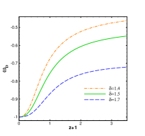
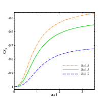
Figure 1: $\omega_{D}$ for some values of $\delta$ as a function of $z$, whenever $\Omega_{D}(z=0)=0.70$ (the upper panel) and $\Omega_{D}(z=0)=0.73$ (the lower panel).

Taking the time derivative of Eq. (7), using Eqs. (10) and (6), and combining the result with Eq. (8), one can obtain

$$\frac{\dot{H}}{H^{2}}=-\frac{3}{2}(1+\omega_{D}+u)\Omega_{D}.$$ (11)

On the other hand, inserting Eq. (6) into Eq. (6), we find that

$$\frac{\dot{H}}{H^{2}}=(1+\omega_{D})\dfrac{3}{2\delta-4},$$ (12)

compared with Eq. (11) to reach at

$$\omega_{D}=\dfrac{u(2-\delta)\Omega_{D}}{1-(2-\delta)\Omega_{D}}-1.$$ (13)

Now, bearing Eq. (9) in mind, this result takes finally the form

$$\omega_{D}=\dfrac{\delta-1}{(2-\delta)\Omega_{D}-1}.$$ (14)

For $\delta<1$, we have $2-\delta>1$ meaning that there is a divergence in the behavior of $\omega_{D}$ happen at the redshift for which $\Omega_{D}=\frac{1}{2-\delta}$. Therefore, the $\delta<1$ case is not suitable in our setup. From Eq. (8), we can easily find that

$$\Omega_{D}^{\prime} =\frac{d\Omega_{D}}{d(\ln a)}=(-2\delta+2)\Omega_{D}\frac{\dot{H}}{H^{2}}.$$ (15)

Combining this result with Eqs. (12) and (14), one obtains

$$\Omega_{D}^{\prime}=3(\delta-1)\Omega_{D}\left(\dfrac{1-\Omega_{D}}{1-(2-\delta)\Omega_{D}}\right),$$ (16)

which finally leads to

$$\Omega_{D}(1-\Omega_{D})^{1-\delta}=\mathcal{C}a^{3(\delta-1)}=\mathcal{C}(1+z)^{3(1-\delta)},$$ (17)

where $\mathcal{C}$ is the integration constant determined by initial conditions. We also used the $1+z=\frac{1}{a}$ relation, where $z$ denotes the redshift, in order to obtain the last equality.

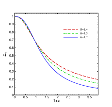
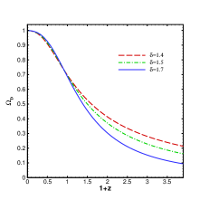
Figure 2: $\Omega_{D}$ for some values of $\delta$. The $\Omega_{D}(z=0)=0.70$ and $\Omega_{D}(z=0)=0.73$ conditions have been used to plot the upper and lower panels, respectively.

Considering some values of $\delta$, the $\omega_{D}$ and $\Omega_{D}$ parameters have been plotted as the functions of the redshift $z$ in Figs. 1 and 2 for the $\Omega_{D}(z=0)=0.70$ (the upper panel) and $\Omega_{D}(z=0)=0.73$ (the lower panel) initial conditions, where $z=0$(or equally a=1) represents the current era. It is easy to see that for $\Omega_{D}\rightarrow 0$ ($\Omega_{D}\rightarrow 1$), we have $\omega_{D}\rightarrow 1-\delta$ ($\omega_{D}\rightarrow-1$). Moreover, if $\delta=2$, then $w_{D}=-1$, a result independent of the value of $\Omega_{D}$. In fact, as it is apparent from Eqs. (6) and (6), this case is mathematically equivalent to the famous cosmological constant model of DE.

We can also calculate the deceleration parameter, defined as

$$q=-1-\frac{\dot{H}}{H^{2}},$$ (18)

by substituting Eq. (14) into Eq. (12) as

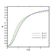
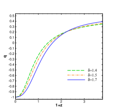
Figure 3: $q$ for some values of $\delta$, when $\Omega_{D}(z=0)=0.70$ (the upper panel) and $\Omega_{D}(z=0)=0.73$ (the lower panel).

$$q=\left(\frac{1}{2}\right)\left[\dfrac{(1-2\delta)\Omega_{D}+1}{1-(2-\delta)\Omega_{D}}\right].$$ (19)

The deceleration parameter $q$ has been plotted for some values of $\delta$ in Fig. 19, where $\Omega_{D}(z=0)=0.70$ (the upper panel) and $\Omega_{D}(z=0)=0.73$ (the lower panel). It is obvious that at $\Omega_{D}\rightarrow 1$ ($\Omega_{D}\rightarrow 0$) limit, we have $q=-1$ ($q=1/2$), a desired asymptotic behavior independent of the value of $\delta$. It is also apparent that, depending on the value of $\delta$, a suitable range for the transition redshift $z_{t}$ (from a decelerated to an accelerated universe) is obtainable ($0.48\leq z_{t}<1$) Riess0 ; Riess ; Riess1 ; Riess2 ; Riess3 ; COL2001 ; COL20011 ; COL20012 ; COL20013 ; HAN2000 ; HAN20001 ; HAN20002 .

The total equation of state parameter is defined as $\omega=P_{D}/(\rho_{D}+\rho_{m})$ leading to

$$\omega=\left(\dfrac{1}{1+u}\right)\omega_{D}=\Omega_{D}\omega_{D},$$ (20)

plotted versus $z$ in Fig. 4. As a desired result, we see that $\omega\rightarrow 0$ ($\omega\rightarrow-1$) with increasing (decreasing) $z$ in full agreement with this fact that the pressureless DM was dominant at the early time in our model.

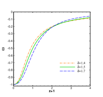
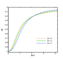
Figure 4: $\omega$ for some values of $\delta$ as a function of $z$, whenever $\Omega_{D}(z=0)=0.70$ (the upper panel) and $\Omega_{D}(z=0)=0.73$ (the lower panel).

Finally, we explore the stability of the THDE model against perturbation by considering its squared sound speed $v_{s}^{2}=\frac{dP_{D}}{d\rho_{D}}$ whose sign determines the stability of the model Peebles20031 . When $v_{s}^{2}<0$ the model is unstable against perturbation. The squared sound speed is written as

$$v_{s}^{2}=\frac{dP_{D}}{d\rho_{D}}=\frac{\dot{P}_{D}}{\dot{\rho}_{D}}=\dfrac{\rho_{D}}{\dot{\rho}_{D}}\dot{\omega}_{D}+\omega_{D}.$$ (21)

Now, using Eqs. (6), (15) and (14), one easily finds

$$\frac{\rho_{D}}{\dot{\rho}_{D}}=\frac{-1}{3H}\left(\dfrac{1-(2-\delta)\Omega_{D}}{2-\delta-(2-\delta)\Omega_{D}}\right).$$ (22)

Taking the time derivative of Eq. (14), we reach

$$\dot{\omega}_{D}=\dfrac{(2-\delta)(1-\delta)H\Omega_{D}^{\prime}}{\left[1-(2-\delta)\Omega_{D}\right]^{2}},$$ (23)

where we used the $\dot{\Omega}_{D}=H\Omega_{D}^{\prime}$ relation obtained from Eq. (15). It can be combined with Eqs. (16), (21) and (22) to reach at

$$v_{s}^{2}=\dfrac{(\delta-1)(\Omega_{D}-1)}{\left[1-(2-\delta)\Omega_{D}\right]^{2}}.$$ (24)

Since $0<\Omega_{D}<1$, the sign of $v_{s}^{2}$ depends on the value of $\delta$. For $\delta>1$, it is clear that $v_{s}^{2}<0$, and the THDE is unstable, while for $\delta\leq 1$ we have $v_{s}^{2}\geq 0$ which implies that THDE with Hubble cutoff is stable against perturbation. But, as it has been argued, the latter leads to a singularity in the behavior of $\omega_{D}$ in our setup.

IV The Universe age

The age of the present universe can be evaluated as

$$t=\int\frac{dtdH}{dH}=\int\frac{1}{\frac{\dot{H}}{H^{2}}}\frac{dH}{H^{2}}$$ (25)

$$=\frac{(\frac{B}{3m_{p}^{2}})^{\frac{1}{2\delta-2}}}{3(1-\delta)}\int\frac{(2-\delta)\Omega_{D}-1}{\Omega_{D}^{\frac{3-2\delta}{2-2\delta}}[1-\Omega_{D}]}d\Omega_{D},$$

where we used the $\frac{dH}{H^{2}}=\frac{(\frac{B}{3m_{p}^{2}})^{\frac{1}{2\delta-2}}d\Omega_{D}}{2(1-\delta)\Omega_{D}^{\frac{3-2\delta}{2-2\delta}}}$ relation as well as Eqs. (12) and (14) to obtain the above result. It finally leads to

$$t=\frac{2(2-\delta)}{3H}\times$$ (26)

$$[1+\big{(}\frac{\delta-1}{2-\delta}\big{)}\ _{2}F_{1}(1,\frac{1}{2(\delta-1)};1+\frac{1}{2(\delta-1)};\frac{BH^{2-2\delta}}{3m_{p}^{2}})],$$

in which ${}_{2}F_{1}(a,b;c;d)$ is the hypergeometric function of the $1$st kind. In order to have an estimation for the order of the age of the current universe ($z=0$), using the second equality of Eq. (25), and Eq. (12), one may write

$$t=\int\frac{1}{\frac{\dot{H}}{H^{2}}}\frac{dH}{H^{2}}\approx\big{(}\frac{1}{\frac{\dot{H}}{H^{2}}}\big{)}\bigg{|}_{z=0}\int\frac{dH}{H^{2}}$$ (27)

$$=\frac{2(2-\delta)}{3H_{0}}\big{(}1-\frac{\omega_{D}(z=0)}{1+\omega_{D}(z=0)}\big{)},$$

where $H_{0}$ is the current value of the Hubble parameter. In this manner, if we consider the initial condition $\omega_{D}(z=0)=-2/3$, then we have $t=1/H_{0}$ for $\delta=3/2$. As another example, for $\Omega_{D}(z=0)=0.70$ and $\delta=1.7$, we have $\omega_{D}\simeq-0.87$ (from the upper panel of Fig. 1) and thus $t\approx 1.5/H_{0}$. A more accurate calculation by using Eq. (25) leads to $t\simeq 0.92/H_{0}$ for this case meaning that Eq. (27) gives true order ($1/H_{0}$) for the universe age. Eq. (27) may also be modified by considering $i$) possible interactions between the cosmos sectors $ii$) other IR cutoffs $iii$) various corrections to the entropy or even $iv$) a combination of the mentioned ways.

V Conclusions

Using the new entropy expression suggested by Tsallis and Cirto non3 , and taking the HDE hypothesis into account HDE ; HDE5 ; HDE17 , we proposed a new holographic dark energy, namely THDE. In addition, we considered a non-interacting flat FRW universe and studied the evolution of the system. $q$, the total equation of state ($\omega$), the equation of state of THDE ($\omega_{D}$), and $\Omega_{D}$ were studied. It has been found out that this model can describe the late time acceleration of the Universe expansion for some values of $\delta$($>1$). It should also be noted that, for $\delta>1$, the model is not stable at the classical level during the cosmic evolution (for all values of $z$). This may be resolved by considering $i$) probable interactions between the cosmos sectors $ii$) other IR cutoffs $iii$) various corrections to the entropy or even $iv$) a combination of the these ways RevH ; wang ; stab . In fact, these considerations may also increase and modify the behavior and predictions (such as the present universe age) of THDE. They are subjects studied at the next steps to become more close to the various properties of THDE, and thus the origin of dark energy.