Self-assembly of polymeric particles in Poiseuille flow: A hybrid Lattice Boltzmann / External Potential Dynamics simulation study

Abstract

We present a hybrid simulation method which allows one to study the dynamical evolution of self-assembling (co)polymer solutions in the presence of hydrodynamic interactions. The method combines an established dynamic density functional theory for polymers that accounts for the nonlocal character of chain dynamics at the level of the Rouse model, the external potential dynamics (EPD) model, with an established Navier-Stokes solver, the Lattice Boltzmann (LB) method. We apply the method to study the self-assembly of nanoparticles and vesicles in two-dimensional copolymer solutions in a typical microchannel Poiseuille flow profile. The simulations start from fully mixed systems which are suddenly quenched below the spinodal line. In order to isolate effects caused by walls, we use a reverse Poiseuille flow geometry with periodic boundary conditions. We identify three stages of self assembly, i.e., initial spinodal decomposition, particle nucleation, and particle growth (ripening). We find that (i) In the presence of shear, the nucleation of droplets is delayed by an amount roughly proportional to the shear rate, (ii) Shear flow greatly increases the rates of particle fusions, (iii) in later stages of self-assembly, stronger shear flows may induce irreversible shape transformation via finger formation, in particular in vesicle systems. The combination of these effects lead to an accumulation of particles close to the center of the Poiseuille flow profile, and the polymeric matter has a double peak distribution centered around the flow maximum.

I Introduction

The study of inhomogeneous polymer systems is a central research field in materials science ^{1; 2}. In particular, systems of diblock copolymers have been studied intensely in the last decades as they exhibit interesting morphologies on the mesoscale ^{3; 4}. Theoretical investigations, numerical studies and computer simulations have led to a good understanding of polymer melts of diblock copolymers and their phase behavior ^{5; 6; 7; 8; 9; 10}.

Specifically, the self-assembly of copolymers in solutions has received increasing interest in the last years. Depending on the polymer structure in copolymer systems, mesoscale structures like lamellae, micelles, vesicles or even more complex structures may assemble ^{11; 12; 13; 14; 15}. Such structures occur in nature and have an important function in cells ¹⁶, and they have a variety of potential applications in (bio)technology, e.g. for encapsulation and transport ¹⁷.

Modeling the self-assembly of such structures on mesoscales is non-trivial and requires coarse-graining techniques ¹⁸. Whereas the self-assembly of single small vesicles from surfactant solutions can be studied by classical all-atom molecular dynamics (MD) ¹⁹, this is not feasible for larger systems. Simulations of the spontaneous self-assembly of surfactant vesicles have resorted to coarse-grained MD ²⁰, Brownian dynamics (BD) ^{21; 22; 23}, dynamic Monte Carlo (MC) ^{24; 25; 26; 27; 28}, dissipative particle dynamics ²⁹ and hybrid MD/multiparticle collision dynamics (MPCD) ³⁰. DPD has also been used to investigate polymersomes ^{31; 32; 33; 34}, however, these studies were restricted to rather short polymers. On the other side of the spectrum, field-based methods such as density functional theory ^{35; 36} and self consistent field theory ^{37; 38} are powerful tools to study self-organizing inhomogeneous polymer systems. Dynamic extensions of these field models ^{39; 40; 41; 42; 15} have given useful insight into the mechanisms of nanoparticle self assembly in polymeric systems ^{43; 44; 14; 45; 46; 47}. However, including fluid flow and hydrodynamic interactions in such studies has remained a challenge.

A number of studies have considered the behavior of vesicles in external flows such as Poiseuille flow or shear flow. They have typically focussed on the deformations of droplets and vesicles in shear flow ^{48; 49; 50; 51; 52; 53; 54; 55} and on lifting forces that determine their lateral position in the channel ^{56; 57; 58; 59; 60}. Most of them were based on a particle description, where the droplets/vesicles are treated as individual (possibly deformable) objects, and they did not address self-assembly.

Other authors have studied the self-assembly of block copolymer melts under shear ^{61; 62; 63}. In agreement with recent dissipative particle dynamics (DPD) simulations ⁶⁴, they found that the shear flow induces morphological rearrangements and favors cylindrical structures that are parallel to the flow ⁶⁴. In these studies, the flow field was imposed and the feedback effect of self-assembly on the instantaneous flow profile was neglected, i.e., hydrodynamic interactions were ignored. However, it is well known that hydrodynamic interactions can influence structure formation in soft matter quite dramatically ⁶⁵, the kinetics is often accelerated and kinetic traps can be avoided ^{66; 67; 15}. To account for such effects, one must use a simulation method that couples, in both directions, the field-based description of the free energy in complex fluids with a hydrodynamic description of fluid flow in a consistent manner.

One such method was recently developed by Zhang and two of us ¹⁵. Unfortunately, the dynamical model did not properly account for the connectivity of the polymers, i.e., monomers were treated as if they moved independently from one another. As a result, kinetic pathways of vesicle self-assembly were observed in simulations that are suppressed in reality. For example, block copolymer vesicles in solutions easily merged by fusion in the simulations ¹⁵, whereas fusions are very rare in reality and in simulations that use a more realistic, albeit purely diffusive dynamical model ^{46; 14; 45}.

In the present study, we propose a hybrid simulation method that combines a nonlocal model for the polymer diffusion, the so-called external potential dynamics (EPD) model ⁴⁰, with the Lattice Boltzmann (LB) method for fluid dynamics ⁶⁸. With this new method we investigate the assembly of mesoscale structures, namely internally structured droplets and vesicles, in a shear flow in the form of two opposite Poiseuille flows.

At equilibrium, several pathways of vesicle formation have been reported from simulations ^{29; 46; 14; 33; 27} and experiments ^{69; 70; 27; 71; 72}. Here, we focus on the nucleation-and-growth pathway which has been observed at low polymer concentration in field-based simulations ^{46; 14}, DPD ³³ and experiments ^{70; 71}. We study the effect of Poiseuille flow on nucleation and ripening of the droplets and vesicles, and on the distribution of polymeric matter across the channel.

By using EPD, which approximates non-local Rouse dynamics (chains move as a whole), we expect to obtain more realistic results for the kinetic pathways of self-assembly, which allows us to identify relevant metastable states. Such transient states could be stabilized, e.g., by crosslinking ”on the fly”. Hence simulations based on the new method not only give insights into the mechanisms of self-assembly under conditions far from equilibrium, but may also help to design experimental strategies for making novel types of nanoparticles which do not correspond to stable equilibrium structures.

The rest of the paper is organized as follows. In Sec. II, we explain the phyiscal background of our new method and how it is implemented. Then we present results of the assembly of droplets and vesicles in polymer solutions in a closed system in Sec. III and in Poiseuille flow in Sec. IV, focussing on nucleation in Sec. IV.1 and on ripening in Sec. IV.2. Our results are summarized in Sec. V.

II Simulation Model and Method

We consider diblock A:B copolymers with A-fraction $q_{A}$, immersed in an explicit solvent S. The copolymers are modeled by Gaussian chains.

The system is treated within polymer density functional theory, hence the free energy is written as a functional of the dimensionless local composition fields $\Phi_{I}(\mathbf{r})$ of species $I$ with $I=A,B,S$ for A-monomers, B-monomers, and solvent particles, respectively. The composition fields $\Phi_{I}$ are normalized such that the actual number density is given by $\Phi_{I}/v$ with the average particle volume $v$ (which is taken to be identical for monomers A,B and solvent). The free energy is then written as ${\cal F}[\Phi]=F[\Phi]/(\beta v)$ ($\beta=1/k_{B}T$ is the Boltzmann constant) with ^{37; 46}

$$F[\Phi] =-\bar{\Phi}_{S}V\ln{(Q_{S}/V\bar{\Phi}_{S})}-\frac{\bar{\Phi}_{P}}{N}V\ln{(Q_{P}N/V\bar{\Phi}_{P})}$$

$$+\int\mathrm{d}\mathbf{r}\>\Big{[}\>\frac{1}{2}\sum_{I,J\neq I}\chi_{IJ}\Phi_{I}\Phi_{J}$$ (1)

$$-\sum_{I}\omega_{I}\Phi_{I}+\frac{\kappa_{H}}{2}(\sum_{I}\Phi_{I}-1)^{2}\Big{]}.$$

Here, $N$ denotes the number of segments per chain, $\bar{\Phi}_{P}$ and $\bar{\Phi}_{S}$ are the average volume fractions of polymer and solvent, $Q_{P}$ and $Q_{S}$ are the partition function for a single polymer chain and the solvent, and the $\omega_{I}$ represent auxiliary ”potential” fields which would generate the same composition fields $\{\Phi_{J}(\mathbf{r})\}$ in a reference system of noninteracting polymers. The last term in Eq. (1) ensures that $\sum_{I}\Phi_{I}\approx 1$ everywhere. For reasons of numerical stability we allow for small deviations and introduce a finite Helfand parameter $\kappa_{H}$. The most important control parameters are the Flory-Huggins parameters $\chi_{IJ}$, which control the interaction strength between different species.

The composition fields $\Phi_{I}$ propagate according to a convection diffusion equation

$$\partial_{t}\Phi_{I}=-\nabla\cdot\textbf{j}_{I}^{D}-\nabla\cdot(\textbf{v}\;\Phi_{I})=:(\partial_{t}\Phi_{I})^{D}+(\partial_{t}\Phi_{I})^{C}$$ (2)

(superscripts $D,C$ refer to the diffusion and convection, respectively), where v is the velocity of the hydrodynamic flow field. We take the flow field to be the same for all components (in contrast to two-fluid models such as Ref. ⁷³). For the first term, the diffusive part, we adopt an adiabatic approximation, according to which the characteristic time scales of internal chain relaxations are much smaller than the relevant diffusive time scales of the system. Hence chains are taken to diffuse as a whole and the diffusive current $\textbf{j}_{I}^{D}$ has the form (originally derived by Maurits et al. )⁴⁰:

$$\textbf{j}_{I}^{D}(\textbf{r})=-D_{I}\sum_{J}\int\mathrm{d}\textbf{r}^{\prime}P_{IJ}(\textbf{r},\textbf{r}^{\prime})\nabla_{\textbf{r}^{\prime}}\frac{\delta F}{\delta\Phi_{J}(\textbf{r}^{\prime})},$$ (3)

Here, $D_{I}$ denotes the diffusion coefficient of species $I$, and the two-body correlator is given by ⁴⁰

$$P_{IJ}(\textbf{r},\textbf{r}^{\prime})=-\frac{\delta\Phi_{I}(\textbf{r})}{\delta\omega_{J}(\textbf{r}^{\prime})}.$$ (4)

To avoid the explicit evaluation of the two-body correlator, we adopt the EPD approximation of Maurits et al. ⁴⁰ and assume that $\nabla_{\textbf{r}}P_{IJ}(\textbf{r},\textbf{r}^{\prime})=-\nabla_{\textbf{r}^{\prime}}P_{IJ}(\textbf{r},\textbf{r}^{\prime})$, which is definitely true in a homogeneous system with $P_{IJ}(\textbf{r},\textbf{r}^{\prime})=P_{IJ}(\textbf{r}-\textbf{r}^{\prime})$. Then the diffusive part of Eq. (2) (the first term on the r.h.s.) can conveniently be rewritten as a local equation for the ”external potentials” $\omega_{I}$ ^{40; 46}. More specifically, we exploit the fact that there exists a unique relation between $\Phi_{J}$ and $\omega_{J}$, hence the time evolution equation (2) can equivalently be written as an equation for $\omega_{I}$, i.e., $\partial_{t}\omega_{I}=(\partial_{t}\omega_{I})^{D}+(\partial_{t}\omega_{I})^{C}$ with

$$\Big{[}\partial_{t}\omega_{I}(\textbf{r})\Big{]}^{D}=-D_{I}\nabla^{2}\frac{\delta F}{\delta\Phi_{I}}.$$ (5)

In our previous work (Zhang et al. ¹⁵), we have used a much simpler Ansatz for the diffusive flow, $\textbf{j}_{I}^{D}=-D_{I}\Phi_{I}(\textbf{r})\nabla\frac{\delta F}{\delta\Phi_{I}(\textbf{r})}$ (local dynamics). This describes a situation where monomers move independently from each other. The present nonlocal model accounts for the fact that monomers in a chain move cooperatively. It should be noted that in systems containing sharp interfaces, the EPD approximation may produce artefacts compared to explicit particle simulations and more sophisticated schemes must be used (S. Qi et al., manuscript in preparation). At weak segregations, however, a systematic study by Reister and Müller has showed that the EPD simulation scheme is superior to the local dynamics scheme and could reproduce the time evolution of structure factors in reference particle simulations on polymer demixing at a quantitative level ^{74; 41}.

In practice, the composition fields $\Phi$ are calculated from the auxiliary potentials $\omega$ as follows ^{37; 41}: One introduces partial partition functions $g(\textbf{r},s)$, which fulfill the modified diffusion equations

$$\partial_{s}g(\textbf{r},s)=R_{G}^{2}\Delta g(\textbf{r},s)-N\omega(\textbf{r},s)g(s,\textbf{r})$$ (6)

$$\partial_{s}g^{\prime}(\textbf{r},s)=R_{G}^{2}\Delta g^{\prime}(\textbf{r},s)-N\omega(\textbf{r},s)g^{\prime}(s,\textbf{r})$$ (7)

Here $s\in[0:1]$ parametrizes the position within a chain, the function $\omega(\textbf{r},s)$ is equal to $\omega_{A}(\textbf{r})$ for $s<q_{A}$, and to $\omega_{B}(\textbf{r})$ otherwise, and $R_{G}$ is the gyration radius of one chain. We solve these equations numerically using a pseudo-spectral method introduced by Tzeremes et al. ⁷⁵

$$g(\textbf{r},s+\mathrm{d}s) =\exp{\left[-\frac{N\omega(\textbf{r},s+\mathrm{d}s)}{2}\mathrm{d}s\right]}\exp{\left[R_{G}^{2}\,\Delta\>\mathrm{d}s\right]}$$ (8)

$$\times\exp{\left[-\frac{N\omega(\textbf{r},s)}{2}\mathrm{d}s\right]}g(\textbf{r},s).$$

The $\exp{\left[\Delta\>\mathrm{d}s\right]}$-part is evaluated in Fourier space (here $\Delta$ is the Laplacian), and the other part is evaluated in real space.

The polymer densities are calculated by integrating the partial partition functions over $s$:

$$\Phi_{A}(\textbf{r}) =\frac{V\>\bar{\Phi}_{P}}{Q_{P}}\int_{0}^{q_{A}}\mathrm{d}s\>g(\textbf{r},s)g^{\prime}(\textbf{r},1-s)$$ (9)

$$\Phi_{B}(\textbf{r}) =\frac{V\>\bar{\Phi}_{P}}{Q_{P}}\int_{q_{A}}^{1}\mathrm{d}s\>g(\textbf{r},s)g^{\prime}(\textbf{r},1-s)$$ (10)

$$\Phi_{S}(\textbf{r}) =\frac{V\>\bar{\Phi}_{S}}{Q_{S}}\exp{\left[-\omega_{S}(\textbf{r})\right]},$$ (11)

where the densities are normalized by the partition functions $Q_{P}=\int\mathrm{d}\textbf{r}\>g(\textbf{r},1)$ and $Q_{S}=\int\mathrm{d}\textbf{r}\>\exp{\left[-\omega_{S}(\textbf{r})\right]}$.

The full convection-diffusion equation (2) is solved by a simple Euler-forward scheme with alternating convection and diffusion steps. The convection steps are most conveniently performed in terms of the composition fields $\Phi$, and the diffusion steps in terms of the auxiliary fields $\omega$ (via Eq. (5)). The calculation of $\phi$ from $\omega$ via Eqs. (6)-(11) is straightforward. The calculation of $\omega$ from $\Phi$ is done iteratively with the conjugate gradients method ⁷⁶.

The fluid dynamics is modeled with a D2Q9 Lattice Boltzmann (LB) environment ^{68; 77}, which is based on a set of discrete velocities $\textbf{c}_{i}$, and a lattice with lattice sites r, populated by a number of fluid particles $n_{i}(\textbf{r})$ with velocities $\textbf{c}_{i}$. The local mass density of the fluid $\rho$ and the flow velocity v are then calculated as $\rho=\sum_{i}n_{i}$ and $\rho\textbf{v}=\sum_{i}n_{i}\textbf{c}_{i}$. The populations $n_{i}$ are propagated with a streaming and a collision step according to

$$n_{i}(\textbf{r}+\textbf{c}_{i}\Delta t,t+\Delta t)=n_{i}(\textbf{r},t)+\Delta_{i}(\textbf{r},t).$$ (12)

In our implementation, we use a multi-relaxation time LB algorithm ^{78; 79}. Since our dynamical model is a mean-field model and thermal fluctuations are not included in the convection-diffusion equation (2), we also do not thermalize the LB modes for consistency.

The thermodynamically driven diffusive flow of the polymers in solution induces fluid flow. To account for this effect, the Navier Stokes equations for a Newtonian fluid have to be extended, either by including an additional stress term of the form $\nabla\tilde{\sigma}$ or, equivalently, a corresponding bulk force term f. We choose the second variant ¹⁵ and write the flow equation in the form

$$\rho\left(\partial_{t}\textbf{v}+\textbf{v}\cdot\nabla\textbf{v}\right)=\textbf{f}-\nabla p+\nabla\sigma^{\prime}.$$ (13)

where $\sigma^{\prime}$ denotes the viscous stress tensor of a Newtonian fluid and $p$ is the pressure. To implement the force coupling in the LB scheme, we follow Ref. ⁷⁹ and extend the collision operator by adding a force contribution

$$\Delta_{i}^{\prime\prime}=a^{c_{i}}\left[\frac{\Delta t}{c_{s}^{2}}f_{\alpha}c_{i\alpha}+\frac{\Delta t}{2c_{s}^{4}}\Sigma_{\alpha\beta}\left(c_{i\alpha}c_{i\beta}-c_{s}^{2}\delta_{\alpha\beta}\right)\right]$$ (14)

with

$$\Sigma_{\alpha\beta} =\frac{1}{2}\left(1+\gamma_{s}\right)\left[\text{v}_{\alpha}f_{\beta}+\text{v}_{\beta}f_{\alpha}-\frac{2}{3}\text{v}_{\gamma}f_{\gamma}\delta_{\alpha\beta}\right]$$ (15)

$$+\frac{1}{3}\left(1+\gamma_{b}\right)\text{v}_{\gamma}f_{\gamma}\delta_{\alpha\beta},$$

where the prefactors $a^{c_{i}}$ are the weight factors of the D2Q9 model ⁶⁸, $c_{s}=\Delta x/\Delta t\sqrt{3}$ is the speed of sound, $\Delta x$ and $\Delta t$ are the lattice constant and the LB time step, and $\gamma_{s},\gamma_{b}$ are the relaxation parameters of the multi-relaxation LB algorithm, which set the shear and bulk viscosity, $\eta$ and $\eta_{B}$, via ⁸⁰

$$\eta=\frac{\Delta t\rho c_{s}^{2}}{2}\frac{1+\gamma_{s}}{1-\gamma_{s}},\qquad\eta_{B}=\frac{\Delta t\rho c_{s}^{2}}{d}\frac{1+\gamma_{b}}{1-\gamma_{b}},$$ (16)

where $d$ is the spatial dimension.

The mechanical force density field $\mathbf{f}$ in Eq. (13), which is to be coupled to LB, is transmitted to the fluid by the monomer segments or solvent particles and should be identical to the force driving the diffusive monomer currents. However, the adiabatic approximation, Eq. (3), creates some ambiguity. From a thermodynamic point of view, the force density should be evaluated directly from the free energy according to ^{81; 42} $\textbf{f}^{\mbox{\tiny TD}}=\sum_{I}\textbf{f}^{\mbox{\tiny TD}}_{I}$ with

$$\textbf{f}_{I}^{\mbox{\tiny TD}}(\textbf{r})=-\frac{1}{\beta v}\Phi_{I}\>\nabla\frac{\delta F}{\delta\Phi_{I}}.$$ (17)

This thermodynamic force drives the local diffusive motion of monomers on very short time scales. In the adiabatic approximation, however, monomers of a chain are taken to move together. Rapid internal chain motions are averaged out, and chains move as a whole, like rigid bodies, driven by the total thermodynamic force acting on each chain. Comparing Eq. (3) with the relation $\mathbf{j}_{I}^{D}/v=\beta D_{I}\mathbf{f}_{I}$ between forces and currents, one finds that this corresponds to an independent monomer motion in an effective force field $\textbf{f}^{\mbox{\tiny eff}}=\sum_{I}\textbf{f}^{\mbox{\tiny eff}}_{I}$ with

$$\textbf{f}_{I}^{\mbox{\tiny eff}}(\textbf{r})=-\frac{1}{\beta v}\sum_{J}\int\mathrm{d}\textbf{r}^{\prime}P_{IJ}(\textbf{r},\textbf{r}^{\prime})\nabla_{\textbf{r}^{\prime}}\frac{\delta F}{\delta\Phi_{J}}(\textbf{r}^{\prime}),$$ (18)

In a mechanically consistent model, the force entering (13) should thus be given by the effective force, Eq. (18), which is the thermodynamic force averaged over the gyration radius. In the present work, we choose this second, mechanically consistent type of force coupling. Similarly, we disregard solenoidal part of $\textbf{f}_{I}(\textbf{r})$ in Eq. (18), since solenoidal contributions to $\mathbf{f}_{I}\propto\mathbf{j}_{I}^{D}$ have no effect on the convection-diffusion dynamics, Eq. (2). In Appendix A, we show that the force fields $\mathbf{f}_{I}$ are in fact purely irrotational within the EPD approximation $\nabla_{\textbf{r}}P_{IJ}(\textbf{r},\textbf{r}^{\prime})=-\nabla_{\textbf{r}^{\prime}}P_{IJ}(\textbf{r},\textbf{r}^{\prime})$ and in particular in homogeneous fluids.

In practice, the force fields are evaluated as follows. We reconstruct the irrotational part of $\mathbf{f}_{I}$ from the change in the composition field resulting from the diffusion step.

$$\big{[}\delta\Phi_{I}(\textbf{r},t)\big{]}^{D} = \Big{[}\Phi_{I}(\textbf{r},t)\!-\!\Phi_{I}(\textbf{r},t-\delta t)\Big{]}^{D}\!\!$$ (19)

$$= -v\beta D_{I}\nabla\cdot\textbf{f}_{I}(\textbf{r},t)\delta t$$

After Fourier transformation (k-space), we obtain an explicit expression for the force

$$\hat{\textbf{f}}_{I}(\textbf{k},t)=\frac{1}{\beta v}\frac{\big{[}\delta\hat{\Phi}_{I}(\textbf{k},t)\big{]}^{D}}{D_{I}\delta t}\frac{i\textbf{k}}{|\textbf{k}|^{2}}$$ (20)

This completes the formulation of our model. The diffusive dynamics of the polymer composition fields is coupled to the fluid flow via the force $\mathbf{f}=\sum_{I}\mathbf{f}_{I}$ in the Navier-Stokes equations, Eq. (13), and the fluid flow is coupled to the polymer dynamics via the convection term in the convection-diffusion equation, Eq. (2). We note that these are the only two couplings between the composition fields and the flow fields in the model. In particular, we do not impose a strict relation between the number densities and the mass density. Instead, the total number density $\sum_{I}\Phi_{I}$ and the mass density $\rho$ are approximately kept constant by separate compressibility terms. This represents an approximation which can be applied in fluids that are roughly incompressible, and where the local mass density is roughly independent of the local composition. A flow chart of the simulation algorithm and additional explanations are given in Appendix C.

Our mean-field scheme does not include thermal fluctuations. Formally, they can be included as in Ref. ¹⁵ by adding Gaussian noise terms in the convection-diffusion equation (2) and in the Navier-Stokes equations (13), which satisfy the fluctuation-dissipation theorem. The noise in the hydrodynamic equations can be implemented in the Lattice Boltzmann framework as described in Refs. ^{15; 79}. The thermodynamically consistent implementation of noise in the convection diffusion equation within the EPD approximation, however, is not trivial and requires special efforts ⁴¹. One can mimick the disordering effect of thermal noise by adding a simplified noise term that just guarantees mass conservation, but violates the fluctuation dissipation theorem ⁴⁶. However, such an approximation should only be used to study the mostly deterministic time evolution of a non-equilibrium systems in the mean-field regime, where the exact structure of the noise does not matter too much. It is not suitable for studying equilibrium distributions and thermally driven processes.

In the next sections, we apply our method to study particle self-assembly in closed systems and in shear flow. These calculations are done in two dimensions. This allows us to cover a large range of shear rates with good statistics (many independent simulation runs), and to study large systems over long times in order to investigate flow-induced shape deformations in late stages of self-assembly. In principle, however, the method is not restricted to two dimensions. In three dimensions, the D2Q9 LB scheme must be replaced by a threedimensional scheme such as the D3Q19 scheme ⁶⁸.

III Particle Self-assembly in Closed Systems

We first consider the self-assembly of copolymeric droplets and vesicles in closed systems without external flows. We choose the units of length, time, and mass such that the radius of gyration $R_{G}$, the diffusion coefficient of the solvent $D_{S}$, and the mass of the solvent $m_{S}$ are unity, which gives the time unit $\tau=R_{G}^{2}/D_{S}$. Furthermore, we set the shear and bulk viscosity to $\eta=\eta_{B}=1R_{G}^{2}/\tau\cdot\rho$ and take the masses of particles to be equal for all species, hence the mass density is $\rho=m_{S}/v$. The parameter combination $1/(\beta v)$ (with the Boltzmann factor $\beta$) would set the noise level in a simulation that includes fluctuations ¹⁵. At the mean-field level considered here, where fluctuations are neglected, the parameters $v$ and $\beta$ do not enter the results. Hence we do not need to specify them here.

To isolate the effect of hydrodynamics, we choose the other model parameters according to a previous study by He et al. ⁴⁶, i.e., $N=17$ with a length fraction $q_{A}=0.882$ of (hydrophobic) A-monomers, $D_{A,B}=D_{S}/N$, $\bar{\Phi}_{P}=0.1$, and the interaction parameters $\kappa_{H}=1.176$, $\chi_{AB}=1.05$, $\chi_{AS}=1.20$. Two values of Flory-Huggins parameters $\chi_{BS}$ are considered, namely $\chi_{BS}=0.75$, which leads to systems of droplets, and $\chi_{BS}=-0.15$, which leads to the assembly of vesicles ^{46; 14}. As the droplets in the first case show structural resemblance to micelles, we will call these particles micelle-shaped droplets and refer to the first case as ”droplet systems”. Systems of the second kind will be called ”vesicle systems”.

The grid spacing $\Delta x$ is chosen $R_{G}/3$ both for the LB part and the solution of the convection-diffusion equation, and the timestep is set to $\Delta t=0.002\tau$. The time step determines the ”lattice velocity” $c=\Delta x/\Delta t$ in the LB system, which is proportional to the speed of sound $c_{s}$, and must hence be chosen small enough that the processes of interest are slow compared to $c$. In our system, we have $R_{g}/c\approx 0.006\tau$, which is much shorter than the time scale of diffusion, $R_{g}^{2}/D_{S}=1\tau$.

The system size is chosen $50R_{G}\times 50R_{G}$ with periodic boundary conditions. The simulation runs start from a perfectly mixed system, which is homogeneous except for a very small random noise which varies from system to system. Apart from this small initial inhomogeneity, there is no further source of noise. Thermal fluctuations are not included, and the simulation runs are completely deterministic. This choice of system setup allows us to make a precise comparison of the evolution of a configuration with and without hydrodynamics, i.e., with and without coupling to the LB simulation.

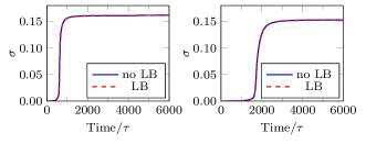
Figure 1: Evolution of $\sigma$ with time $t$ (units $\tau$) in a system with hydrodynamics (dashed red curve: EPD convection-diffusion equation coupled to LB simulation), and a corresponding system (same initial conditions) without hydrodynamics (full blue curve: pure EPD simulation). Left: droplet system ($\chi_{BS}=0.75$), right: vesicle system ($\chi_{BS}=-0.15$)

Following Ref. ⁴⁶, we introduce a quantity which quantifies the mixing of solvent and polymers:

$$\sigma(t)=\frac{1}{V}\int\mathrm{d}\textbf{r}|\Phi_{P}(\textbf{r},t)-\bar{\Phi}_{P}|,$$ (21)

where $V$ is the volume of the system and $\Phi_{P}=\Phi_{A}+\Phi_{B}$ the volume fraction of polymers. The state $\sigma=0$ corresponds to a perfectly mixed system, and increasing $\sigma$ signalizes segregation. 1 shows a typical time evolution $\sigma(t)$ in systems set up as described above. At the beginning, the system decomposes slowly from an initially almost perfectly mixed state. The speed of the segregation process increases until the system reaches a ”nucleation stage”, at which $\sigma$ shows a sudden increase. Finally $\sigma$ saturates, which denotes the ripening stage. In agreement with the results from He et al. ⁴⁶, we find that nucleation takes place much earlier in systems with $\chi_{BS}=0.75$, where the final structures are micelle-shaped droplets, compared to systems with $\chi_{BS}=-0.15$, where vesicles can emerge.

We have also analyzed how the number of particles changes with time after the initial nucleation stage (data not shown). Both in the systems with and without hydrodynamics, it remains roughly constant in the vesicles systems with $\chi_{BS}=-0.15$, and decreases in the droplet systems with $\chi_{BS}=0.75$. In the latter case, large particles are found to grow at the expense of smaller ones until some of the smaller ones completely dissolved. Fusions of particles are never observed, neither in systems without nor with hydrodynamics.

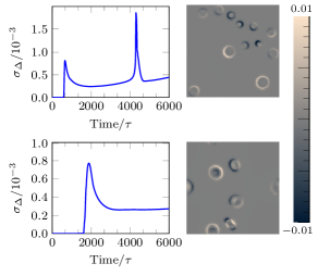
Figure 2: Evolution of $\sigma_{\Delta}$ with time $t$ (left, units $\tau$) in droplet systems ($\chi_{BS}=0.75$, top) and vesicle systems ($\chi_{BS}=-0.15$, bottom) with corresponding difference snapshots of $\Phi_{P}^{LB}(\textbf{r})-\Phi_{P}^{NLB}(\textbf{r})$ (right) at $t=2000\tau$ in the droplet system and $t=3000\tau$ in the vesicle system. The values of the difference are confined to a very narrow regime between from $-0.01$ (blue) and $0.01$ (beige).

In 1, the curves of $\sigma(t)$ for systems with hydrodynamic interactions (where the EPD simulation is coupled to a LB simulation) and without (no coupling) are practically indistinguishable. To further quantify the influence of hydrodynamics on self-assembly, we have examined the polymer structure factor at different times (data not shown). However, in the time range covered by the simulation, the structure factors of systems with and without hydrodynamic coupling were practically identical. Hence we introduce another, more sensitive quantity $\sigma_{\Delta}$, which allows to elucidate local effects of hydrodynamic flows. It integrates over the local absolute difference of the dimensionless polymer distribution $\Phi_{P}^{LB}(\textbf{r})$ in systems with coupled LB simulation, and the corresponding distribution $\Phi_{P}^{NLB}$ in systems without LB coupling (but identical initial conditions) and is defined as

$$\sigma_{\Delta}=\frac{1}{V}\int\mathrm{d}\textbf{r}|\Phi_{P}^{LB}(\textbf{r})-\Phi_{P}^{NLB}(\textbf{r})|.$$ (22)

Results for an example of a droplet and vesicle system are shown in 2. Over all, $\sigma_{\Delta}$ is very small (of order $10^{-3}$). It starts at zero and then exhibits a first peak up to around $0.001$ around the time where nucleation sets in. Then, $\sigma_{\Delta}$ decreases to values below $0.0005$ and levels off, but may occasionally show further peaks which correspond to singular events. For example, the second peak in 2, top, coincides with the dissolution of a droplet.

The local difference plots on the right side of 2 give further insight into the effect of hydrodynamics on phase separation. In the droplet system, the larger droplets are surrounded by beige coronae and the smaller systems by blue coronae, indicating that the growth of large droplets and the shrinking of smaller droplets is slightly accelerated in the presence of hydrodynamics. A more quantitative analysis of difference plots such as 2 showed that fluid dynamics generates a speedup of the order of one percent. This is much less than in our previous study using local dynamics ¹⁵, and in a recent study of self-assembly of small molecules ⁶⁷. Hence, we conclude that hydrodynamic flows have no significant effect on structure formation in our polymer solutions. The flow fields generated by the polymer diffusion seem to be too small to have large feedback effects on the polymer concentration fields.

As already mentioned earlier, the self-assembly of vesicles in the absence of hydrodynamic flows had been studied earlier by He et al. ⁴⁶ using nonlocal, cooperative dynamics, and by Zhang et al. ¹⁵ using local dynamics. Our results here agree with those of He et al. ⁴⁶, who found that fusion of particles is suppressed once the particles have reorganized themselves internally such that they are surrounded by a hydrophilic corona of B-monomers. In contrast, Zhang et al. ¹⁵ did observe particle fusion events, hence the corona seems to affect the kinetics only if the monomers move cooperatively.

Zhang et al. ¹⁵ also studied the effect of hydrodynamic interactions and found that self-assembly was accelerated particularly in the late stages. The main effect seemed to be the acceleration of fusion events. Our present results show that hydrodynamic flows have only a very small effect on the kinetics of particle assembly, if particle fusion is kinetically suppressed.

IV Particle Self-assembly in Poiseuille Flow

Next we investigate the effect of shear flow on the kinetics of self-assembly. We mimick an experimental situation where micelle-shaped droplets and vesicles self-assemble in thin channels, e.g., in a microfluidic device. However, we are not interested in boundary effects here. To eliminate them, we follow Refs. ^{82; 83} and create a system of opposite Poiseuille flows with periodic boundary conditions (reverse Poiseuille flow). This is done by applying a bulk force of the form

$$f_{x}(y)=\begin{cases}-\mbox{$f_{0}$}\qquad y<L_{y}/2\\ +\mbox{$f_{0}$}\qquad y\geq L_{y}/2\end{cases}$$ (23)

in $x$-direction to the fluid. The theoretical prediction for the resulting velocity field (from the Navier Stokes equations) is:

$$v_{x}(y)=-\frac{\mbox{$f_{0}$}}{2\eta}\left(y-\frac{L_{y}}{2}\right)\left(\left|y-\frac{L_{y}}{2}\right|-\frac{L_{y}}{2}\right)$$ (24)

Here $L_{y}$ denotes the $y$-size of the system and $\eta$ is the shear viscosity. The resulting shear rate $\dot{\gamma}=\frac{\partial v_{x}}{\partial y}$ is a linear function in $y$ with the form

$$\dot{\gamma}=\frac{\mbox{$f_{0}$}}{2\eta}\left(\frac{L_{y}}{2}-2\left|y-\frac{L_{y}}{2}\right|\right)$$ (25)

In the following, forces will be given in units of $f^{*}=\rho R_{G}\tau^{-2}$. The amplitude of the force field in our simulations ranges from $\mbox{$f_{0}$}=1\cdot 10^{-5}f^{*}$ to $\mbox{$f_{0}$}=1\cdot 10^{-3}f^{*}$. With these forces, we reach Reynolds numbers up to $2$ and stay in the regime of low Reynolds numbers. Moreover, the shear rate is sufficiently small that real polymers with radius of gyration $R_{G}$ and diffusion constant $D_{P}$ would not deform, which provides a justification for our adiabatic approximation. (Real polymers with Rouse time $\tau_{R}=\frac{2}{\pi^{2}}\frac{R_{G}^{2}}{D_{P}}$ would have Weissenberg numbers below $Wi=\tau_{R}\dot{\gamma}<0.04$ in our shear flows, and polymer deformations become important for $Wi>1.3$ ⁸⁴.)

We will refer to systems with $\mbox{$f_{0}$}<3\cdot 10^{-5}f^{*}$ as ”weakly sheared”, systems with $3\cdot 10^{-5}f^{*}\leq\mbox{$f_{0}$}\leq 3\cdot 10^{-4}f^{*}$ as ”moderately sheared”, and even higher $f_{0}$ as ”strongly sheared”. The model parameters and the initial simulation setup are the same as in the previous section. We will again compare ”droplet systems” with $\chi_{BS}=0.75$ with ”vesicle systems” with $\chi_{BS}=-0.15$ and use simulation boxes of size $50R_{G}\times 50R_{G}$. For bulk forces up to $\mbox{$f_{0}$}=5\cdot 10^{-5}f^{*}$, we average over 100 independent runs per parameter set and otherwise, over 50 runs. The systems were initialized with the flow field defined by Eq. (24). Hence the force field just has to conserve the flow field during the simulation run.

We will first discuss the initial stage of self-assembly where the first nuclei appear (nucleation stage, Sec. IV.1), then analyze the effect of shear on the ripening stage (Sec. IV.2), examine the development of the particle shapes (Sec. IV.3) and the characteristic relaxation times (Sec. IV.4), and finally study the lateral migration of particles and/or polymeric matter across the channel (Sec. IV.5).

IV.1 Nucleation Stage

We begin with investigating the first stage of particle assembly, where nuclei initially form. We call this stage ”nucleation stage”, even though the process of self-assembly is deterministic in our system and not driven by random thermal fluctuations (which are not included in our mean-field treatment). As discussed in earlier work, the nuclei formation is triggered by spinodal decomposition in this case ^{46; 85}. During an initial ”incubation time”, spinodal concentration fluctuations build up until they become large enough that nuclei start to form throughout the system almost simultaneously. Here we study how the number of these nuclei depends on the strength of the shear flow. Thus we count the number of particles right after the nucleation stage, where ”particles” are defined as connected clusters of lattice sites with local polymer volume fractions above $\Phi_{P}\geq 0.5$. Specifically, we determine the particle density $n_{p}$, i.e., the average number of particles per system divided by the system size. The results are shown as a function of $f_{0}$ in 3.

Figure 3: Maximum average particle density during the self-assembly process vs. bulk driving force $f_{0}$ in units of $f^{*}$. Left: vesicle systems ($\chi_{BS}=-0.15$), right: droplet systems ($\chi_{BS}=0.75$)

Small shear flows have little influence on the densities of nuclei. If the force amplitude $f_{0}$ exceeds a certain threshold $f_{0,c}$, the particle densities start to decrease significantly with increasing $f_{0}$. The threshold is much smaller in the ”vesicle systems” with $\chi_{BS}=-0.15$ ($\mbox{$f_{0,c}$}\sim 1\cdot 10^{-4}f^{*}$) than in the ”droplet systems” with $\chi_{BS}=0.75$ ($\mbox{$f_{0,c}$}\sim 2.5\cdot 10^{-4}f^{*}$). Thus, the nucleation of compact particles made of hydrophobic polymers is less affected by shear flow than the nucleation of more open particles made of polymers that also contain strongly hydrophilic blocks.

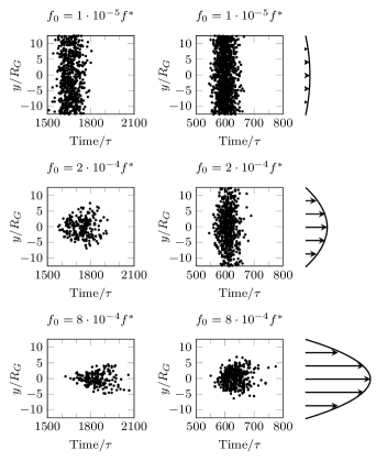
Figure 4: Scatter plot of nucleation events (in all simulations) in the coordinate plane of time vs. $y$ ($y=0$ corresponds to the center of the Poiseuille flow – see the flow profiles in the outer right column) for examples of weakly sheared systems (top), moderately sheared systems (middle), and strongly sheared systems (bottom) with bulk force amplitudes $f_{0}$ as indicated. Left column: vesicle systems ($\chi_{BS}=-0.15$), right column: droplet systems ($\chi_{BS}=0.75$).

Next we examine the distribution of nucleation events across the channel (in the $y$-direction perpendicular to the flow). 4 shows scatter plots of nucleation events in the plane of time vs. $y$-coordinate relative to the center of the Poiseuille flow (denoted $y=0$) for different force amplitudes $f_{0}$ and our two choices of $\chi_{BS}$. Here nucleation events in the upper and lower regions of the simulation box with opposite Poiseuille flows are shown together in one graph. For small $f_{0}$, nucleation events are distributed evenly across the channel. For larger $f_{0}$, nucleation preferably takes place in the area of lowest shear rate close to $y=0$. 5 shows examples of simulation snapshots (polymer density plots) for weak and strong shear flow right after the nucleation stage. In the case of strong shear flow, the nuclei are close to the center of the Poiseuille flow. In systems with weak shear flow, no such preference can be observed.

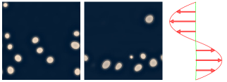
Figure 5: Polymer density plot right after the nucleation stage at $t=700\tau$ in droplet systems ($\chi_{BS}=0.75$) and force amplitude $\mbox{$f_{0}$}=1\cdot 10^{-5}f^{*}$ (left snapshot) and $\mbox{$f_{0}$}=8\cdot 10^{-4}f^{*}$ (right snapshot). Corresponding flow profile is shown on the right.

4 also shows that nucleation events are more focussed at the center of the flow in vesicle systems (left) than in droplet systems (right). Let us consider, for example, the histogram of nucleation events in vesicle systems at force amplitude $\mbox{$f_{0}$}=2\cdot 10^{-4}f^{*}$, which features a broad peak at the center and almost no counts at positions $|y|>7R_{G}$. To reach a similar level of focussing in the micellar systems, one has to increase the force amplitude by roughly a factor of four up to $\mbox{$f_{0}$}\sim 8\cdot 10^{-4}f^{*}$. Hence droplets can also assemble in regions of higher local shear, whereas for vesicles this is unlikely.

Below we will see that the polymer composition profile in the $y$-direction changes during the ripening stage and a double-peak structure emerges at late times. During the nucleation stage, this structure cannot yet be seen.

Next we examine the distribution of nucleation events in time. Already 4 shows clearly that the nucleation stage is delayed if the shear flow is increased. Furthermore, the width of the distribution of the nucleation events in time is much broader in the vesicle systems than in the droplet systems. To quantify this observation, we fit the distribution of nucleation events in time by a Gaussian distribution. The fit matches the data quite well, especially in systems with higher force amplitudes $f_{0}$, where we get reduced $\chi^{2}$ values of the order 1-5. The first moment of the Gaussian gives the characteristic time of the nucleation stage and is shown as a function of $f_{0}$ in 6. Both in vesicle and droplet systems, the nucleation stage is shifted to later times if shear flow is applied. The shift first increases with $f_{0}$ and then saturates at large $f_{0}$, due to the fact that nucleation events are confined to the low-shear center of the flow profile at such force amplitudes.

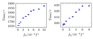
Figure 6: Time of the nucleation stage as a function of force amplitude $f_{0}$ in units of $f^{*}$. Left: vesicle systems ($\chi_{BS}=-0.15$), right: droplet systems ($\chi_{BS}=0.75$)

Looking at 4 more closely, it is apparent that the time and $y$-coordinate of nucleation events are correlated. For weak shear flow, nucleation is homogeneous in $y$. For moderate shear flow, the scatter plots have some resemblance with arrowheads pointing in the direction of small times, i.e., nucleation events first take place close to the center of the Poiseuille flow, and then become increasingly likely in areas with higher local shear stress. To discuss these correlations more quantitatively, we calculate the correlation coefficient of the coordinates $(t,y)$ of nucleation events, defined as

$$c_{t,y}=\frac{\langle(t-\langle t\rangle)(|y|-\langle|y|\rangle)\rangle}{\sqrt{\langle(t-\langle t\rangle)^{2}\rangle\langle(|y|-\langle|y|\rangle)^{2}\rangle}}$$ (26)

Here, $\langle...\rangle$ denotes the statistical average. $c_{t,y}$ is equal to $1$ if $t$ and $y$ are perfectly correlated and zero if there is no correlation. 7 shows the results as a function of force amplitude $f_{0}$. We find that the time and position of nucleation events in Poiseuille flow are uncorrelated for small shear flows, but they become correlated as the force amplitude $f_{0}$ increases. In practice, this means that the distribution of nucleations gradually broadens with time (see 4). The correlation for vesicle systems and droplet systems is comparable.

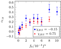
Figure 7: Correlation coefficient of time and $y$-coordinate of nucleation events as a function of force amplitude $f_{0}$ in units of $f^{*}$. Blue: vesicle systems ($\chi_{BS}=-0.15$), red: droplet systems ($\chi_{BS}=0.75$)

We can also use our simulation data to investigate the relation between the local shear rate of nucleation and the local delay time. To this end, we bin the histograms in 4 in the $y$-direction and determine the mean delay time as a function of the local shear rate, for all considered force amplitudes $f_{0}$, in the vesicle and droplet systems. The results are combined in 8. Especially for larger shear rates and in the vesicle systems, the data roughly collapse on a single almost straight line, i.e., the local nucleation time is roughly a linear function of the local shear rate. At low shear rates, the data spread out due to the effect of lateral polymer diffusion. In the droplet systems where the effect of local shear on the nucleation time is much weaker, the collapse is less clear. Nevertheless, the local shear and the local nucleation time are still strongly correlated.

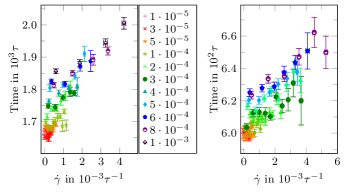
Figure 8: Mean time of nucleation events vs. local shear rate in Poiseuille profiles for different driving force amplitudes $f_{0}$ as indicated (in units of $f^{*}$) in vesicle systems with $\chi_{BS}=-0.15$ (left) and droplet systems with $\chi_{BS}=0.75$ (right).

These findings are consistent with experimental studies on spinodal decomposition and structure formation in polymer mixtures in Couette flows ^{86; 87; 88}. Here, it was found that applying shear flows has a similar effect on the length and time scales of spinodal decomposition than shifting the spinodal line towards lower temperatures ⁸⁸. If we adopt this interpretation, it follows that local shear effectively shifts our system closer to the spinodal line, which in turn increases the characteristic time scale of spinodal decomposition ⁸⁹ and hence the ”incubation” time for nucleation ⁴⁶.

In sum, we find that shear flow significantly affects the droplet and vesicle self-assembly in the nucleation stage. It affects both the time frame and the preferred location of nucleation events. The central observation is that nucleation is delayed in the presence of shear. This observation can account for all findings reported here at a qualitative level: Due to the shear-dependent delay, nucleation events are unevenly distributed in Poiseuille flow. They first emerge in regions of low shear stress (the center of the flow profile), and then gradually also populate regions with higher local stress. At the same time, the existing nuclei grow by incorporating copolymers from solution. The process stops when the remaining level of free copolymers is so low that no further nucleation events take place. If the force amplitude is strong, the nucleation stage is completed before any nucleation events have taken place in the outer regions of the profile. As a result, strongly sheared systems contain fewer nuclei than weakly sheared systems ( 3) and their nuclei are concentrated around the center of the profile (4). These effects are more pronounced in vesicle systems than in droplet systems.

IV.2 Ripening stage: Evolution of particle number

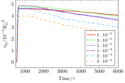
Figure 9: Average particle number density in droplet systems ($\chi_{BS}=0.75$) as a function of time in units of $\tau$ for different force amplitudes $f_{0}$ as indicated (units $f^{*}$).

After the initial nucleation stage, the particle number remains constant or decreases steadily. We will now focus on the evolution of the particle number in this second, ”ripening” stage. We first consider the droplet systems with $\chi_{BS}=0.75$ (9). In these systems, a ripening process reminiscent of classical Ostwald ripening takes place: Large particles tend to grow at the cost of smaller ones, since they have an energetically more favorable surface to volume ratio. The equilibrium state in these systems (close systems without flows) is a single phase separated droplet in solution. Already in the absence of shear, the system evolves slowly towards this final state.

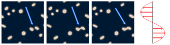
Figure 10: Series of snapshots in a droplet system ($\chi_{BS}=0.75$) with force amplitude $\mbox{$f_{0}$}=2\cdot 10^{-4}f^{*}$ at times $t=3350\tau$, $t=3450\tau$ and $t=3550\tau$, showing the fusion of two particles with almost equal size (see blue arrows). Right panel indicates the shape of the flow profile.

If shear flow is applied, the particle number decreases more rapidly. A closer inspection shows that this is not due to an acceleration of ripening, but due to particle fusions. As discussed in Sec. III, fusion is suppressed in fluids at rest. Under the influence of shear, fusion events become possible. An example is shown in 10.

To analyze the ratio of particle fusions and particle dissolutions as a function of shear strength, we must define criteria that distinguish between two types of event – particle traces getting lost due to particle dissolution or due to fusion. This is done as follows: First, we exploit the fact that only particles close to each other can fuse. Therefore, one criterion for a fusion event is that two particles $i$ and $j$ with a distance less than a threshold $d_{ij}$ must vanish at the same time. The threshold is chosen $d_{ij}=2.5(R_{i}+R_{j})$, where $R_{i,j}$ is the radius of a spherical particle with the same polymer content as particle $i,j$, and the factor $2.5$ accounts for the fact that particles may be deformed in shear flow.

In some rare cases it may happen that the sizes of two fusion partners are so different, that only one of them vanishes and the other one remains nearly unaffected. To distinguish between fusion and dissolution of particles in such cases, we apply the second criterion that only those events are counted as fusion, where the vanishing particles have an area larger than $3.3\>R_{G}^{2}$. If a particle has an area below this threshold before disappearing, we assume that it has dissolved.

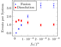
Figure 11: Average number of fusions (blue) and average number of particle dissolutions per system (red) as function of $f_{0}$ (units $f^{*}$) in droplet systems ($\chi_{BS}=0.75$).

Using these criteria, we have determined the fusion and dissolution events in droplet systems ($\chi_{BS}=0.75$) at low and moderate shear rates. The results are shown in 11. We find that the number of particle dissolutions is almost independent of $f_{0}$. In contrast, the number of particle fusions increases with $f_{0}$ and dominates for $\mbox{$f_{0}$}>5\cdot 10^{-5}f^{*}$. In systems with moderate shear, it is 3-4 times larger than the number of particle dissolutions.

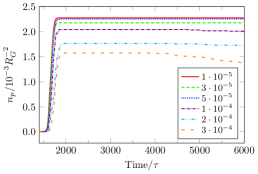
Figure 12: Average particle number density in vesicle systems ($\chi_{BS}=-0.15$) as a function of time in units of $\tau$ for different force amplitudes $f_{0}$ (units $f^{*}$).

Next we examine the evolution of the number of particles in the vesicle system ($\chi_{BS}=-0.15$). The results are shown in 12. In contrast to the droplet system, ripening is not observed in these systems (as already noted in Ref. ⁴⁶). In the absence of shear, the particle number does not change with time. Under the influence of shear, it decreases, and this is the result of particle fusions.

As discussed earlier and in Ref. ⁴⁶, fusion of micelle-shaped droplets and vesicles is prevented in fluids at rest by the hydrophilic corona surrounding the particles. Shear distorts the particles and disrupts the corona, and as a result, fusion becomes possible. We find that even weak shear flows can deform particles significantly. This will be discussed in the next section.

IV.3 Particle Shape

Next we consider the influence of shear on the shapes of particles. In our systems with our model parameters, isolated particles at equilibrium tend to be perfectly round. In systems with more than one particle, the particles influence and deform each other even without getting into contact. In this section, we study how the particle shapes change if the particles are exposed to external shear flow.

The shape of a particle can be characterized by the tensor of gyration ⁹⁰. As the polymer distributions inside a particle are not perfectly uniform in our case, we weight the distances between the different lattice sites $i$ and $j$, which belong to a particle, with their polymer densities $\Phi_{P}(\textbf{r}^{i})$ and $\Phi_{P}(\textbf{r}^{j})$:

$$G_{nm}=\frac{1}{2{\cal N}^{2}}\sum_{i}\sum_{j}\Phi_{P}(\textbf{r}^{i})\Phi_{P}(\textbf{r}^{j})(r_{n}^{i}-r_{n}^{j})(r_{m}^{i}-r_{m}^{j})$$ (27)

Here, $\cal N$ denotes the polymer content of the particle, and the sum runs over all lattice sites $i,j$ with $\Phi_{P}(\textbf{r}_{i,j})\geq 0.5$. By diagonalizing the tensor one obtains the eigenvalues $\lambda_{-}$ and $\lambda_{+}$, from which the acircularity $c$ and the radius of gyration $R$ can be derived,

$$c=\lambda_{+}-\lambda_{-},\quad R=\sqrt{\lambda_{+}+\lambda_{-}}$$ (28)

Here, we will consider the relative acircularity, defined as ⁹⁰:

$$c_{rel}=\frac{c^{2}}{R^{4}}$$ (29)

The relative acircularity is zero for perfectly circular particles and one if the long axis is infinitely longer than the short axis. Thus, it can be interpreted as the level of the particle deformation in shear flow, and used to characterize both droplets and vesicles.

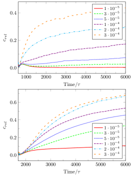
Figure 13: Average relative acircularity of particles as a function of time (units $\tau$) in droplet systems with $\chi_{BS}=0.75$ (top) and vesicle systems with $\chi_{BS}=-0.15$ (bottom) for different force amplitudes $f_{0}$ (units $f^{*}$) as indicated.

In weakly sheared droplet systems (13 top, $\mbox{$f_{0}$}<3\cdot 10^{-5}f^{*}$), the relative acircularity first increases and then drops again. It reaches a maximum during the nucleation stage. This is because freshly nucleated particles cannot grow isotropically if they are close to each other, hence they deform slightly. At later times, they gradually drift away from each other and become more spherical, which lowers the relative circularity again. At the lowest force amplitude, $\mbox{$f_{0}$}=1\cdot 10^{-5}f^{*}$, the final relative acircularity of the particles stays at a very low level. Thus we can conclude that weak shear flow has no significant effect on the shape of droplets in systems where the A- and B-monomers are both strongly solvophobic. At moderate shear, the relative acircularity becomes more pronounced and the shape of the curve changes (13 top, $\mbox{$f_{0}$}>3\cdot 10^{-5}f^{*}$). After an initial relatively rapid increase in the nucleation stage, $c_{rel}$ continues to grow more slowly at later times.

In the vesicle systems, shear flow is found to have a pronounced effect on $c_{rel}$ of particles for all considered shear rates, and $c_{rel}$ keeps increasing steadily at late times even in the system with lowest shear ($\mbox{$f_{0}$}=1\cdot 10^{-5}f^{*}$). Hence particles in vesicle systems can be deformed much more easily than particles in droplet systems. We will now analyze this in more detail.

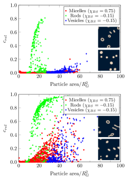
Figure 14: Scatter plot of particle characteristics in the plane of particle area (units $R_{g}^{2}$) vs. relative acircularity in vesicle systems with $\chi_{BS}=-0.15$ (green: rods, blue: vesicles) and droplet systems with $\chi_{BS}=0.75$ (red: micelle-shaped droplets) at time $t=6000\tau$ for force amplitude $\mbox{$f_{0}$}=1\cdot 10^{-5}f^{*}$ (top) and $\mbox{$f_{0}$}=5\cdot 10^{-5}f^{*}$ (bottom). The inset shows snapshots from corresponding simulations at $\chi_{BS}=-0.15$ (top) and $\chi_{BS}=0.75$ (bottom)

One quantity that clearly influences the relative deformability of a particle is its size. Here we will examine the particle area, which we define as the area covered by a particle (interiors of hollow particles excluded), and calculate it according to a procedure described in Appendix B. The average particle area is much larger in vesicle systems than in droplet systems. One might suspect that this is the main reason for their higher deformability. To investigate this possibility, we have constructed scatter plots of particle size vs. relative particle acircularity for fixed (late) simulation time and force amplitude $f_{0}$. Two examples are shown in 14. Each symbol corresponds to one particle in either a droplet or a vesicle system. In addition, we distinguish between hollow and filled particles in the vesicle systems. For reasons that will become clear below, we will refer to the latter ones as ”rods”.

In systems with small or moderate $f_{0}$, the regions in the area-acircularity plane where certain particles exist and regions where they apparently cannot exist are clearly separated. If particles are very small, the range of accessible acircularities is generally very limited, i.e., they remain close to spherical. This observation is in good agreement with early work on fluid droplets immersed in another fluid ⁹¹. For larger particle areas, the diagram displays a steep transition, beyond which the acircularity limit is close to one. This limit is reached by a special class of particles in the vesicle systems, which differ from regular vesicles in that they do not enclose solvent (green triangles in 14), indicating that they correspond to elongated micelles (see also the snapshots in 14). In three dimensions, they could correspond to either wormlike or disklike micelles. Experimental observations suggest that shear flows with uniform shear rate can induce shape transformations from vesicles into wormlike micelles ⁵⁵. Therefore, we will call these elongated structures ”rods” hereafter.

The other categories of particles (red spheres and blue diamonds) have much lower acircularity. A very small number of symbols lie outside the domain of typically ”allowed” acircularities. They correspond to particles that have just emerged from a fusion event and are still highly non-circular. At later times, they relax and become circular again. Interestingly, the accessible range of acircularities for vesicles is smaller than that for droplets with comparable area. Hence, contrary to expectations, we find that vesicles show more resistance to deformations than micelle-shaped droplets. Nevertheless, the total relative acircularity of particles is higher for vesicle systems than for droplet systems (13) due to the contribution of the rods.

The acircularity limits for vesicles and micelle-shaped droplets are found to depend strongly on the force amplitude $f_{0}$. If $f_{0}$ is very small, as in 14 (top), all particles except the rods are close to spherical. If $f_{0}$ is moderate, as in 14 (bottom), the particles can deform more strongly. Moreover, vesicles may develop ”fingers” (see the snapshots in 14 (bottom)). For large shear flows, i.e., large $f_{0}$, there are almost no limitations on acircularity (15). Only very small particles remain circular.

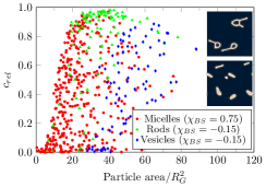
Figure 15: Same as 14 for force amplitude $\mbox{$f_{0}$}=3\cdot 10^{-4}f^{*}$ at time $t=3000\tau$ for droplet systems ($\chi_{BS}=0.75$) and $t=4500\tau$ for vesicle systems ($\chi_{BS}=-0.15$).

We should note that 15 differs from 14 in that it does not show the size-acircularity distribution at the end of a simulation, but at an earlier time where the average acircularity still evolves strongly with time, especially in the vesicle system. This is because at later times, more and more vesicles turn into rod particles via an intermediate state of vesicles with fingers (see inset of 15), such that there are no vesicles left for the analysis. The rod particles then simply maximize the relative acircularity. Similar shape transformations of vesicles are also observed at lower shear rates.

To analyze this more quantitatively, we will now focus on the vesicle systems and investigate the fraction of vesicles with respect to the total number of particles (vesicles and rods) as a function of time. The data are shown in 16. In weakly sheared systems ($\mbox{$f_{0}$}\leq 3\cdot 10^{-5}f^{*}$), the fraction of vesicles in the system rises monotonically and reaches a plateau at late times at around 0.6. A small increase of the shear rate shifts the plateau to slightly lower values, but does not destroy it. Once formed, most vesicles hence tend to remain vesicular. However, this is no longer true in moderately or strongly sheared system. Here, the fraction of vesicles reaches a peak shortly after the nucleation stage, whose height may even exceed the value of 0.6 reached in the weakly sheared systems: Since the number of nuclei is reduced in the presence of shear flow (see Sec. IV.1), particles grow larger and are more likely to turn into vesicles. At later times, the fraction of vesicles drops. This is because the existing vesicles first develop fingers and then eventually turn into rodlike particles. For even more strongly sheared systems (data not shown), the height of the maximum decreases and the rate with which vesicles disappear increases further.

Thus we conclude that in the vesicle system, the particle assembly in Poiseuille flow proceeds in three stages: (i) Nuclei form. (ii) Nuclei grow and turn into vesicles, much like in the closed system without flow ⁴⁶. (iii) Vesicles may develop fingers which then grow and may eventually transform the vesicle into a rod. The rate at which such fingers appear increases with increasing shear rate. However, fingering was observed for all shear rates, even (rarely) in the most weakly sheared systems. At the end of an infinitely long simulation, strongly sheared systems will presumably only contain rods. At finite times, one has a mixture of droplets, vesicles, and rods.

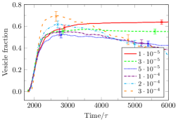
Figure 16: Vesicle fraction in systems with $\chi_{BS}=-0.15$ vs. time (in units of $\tau$) for different force amplitudes $f_{0}$ (in units of $f^{*}$) as indicated. The total number of particles entering this statistics is about $200$ for $\mbox{$f_{0}$}\geq 1\cdot 10^{-4}f^{*}$ and $400$ for $\mbox{$f_{0}$}\leq 5\cdot 10^{-5}f^{*}$.

IV.4 Characteristic relaxation times

The deformability of particles in shear flow should depend on their relaxation time $\tau_{d}$, which sets the relevant mesoscopic timescale in the system. More specifically, we expect that shear flow starts to have a significant effect on particles once the dimensionless shear rate, $\tau_{d}\dot{\gamma}$, becomes of order unity. Assuming that $\tau_{d}$ increases with particle size, this would explain why larger particles deform more easily than smaller particles. To test this assumption, we will now examine the characteristic relaxation times $\tau_{d}$ of the self-assembled particles in our systems. They were measured by taking configurations of moderately sheared systems, stopping the flow in an instant, and letting the particles relax. The relaxation of the acircularity with time was then fitted to a single exponential, $c(t)=c_{0}\exp(-t/\tau_{d})$.

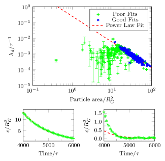
Figure 17: Top: relaxation parameter $\lambda_{d}$ (in units of $1/\tau$) in droplet systems ($\chi_{BS}=0.75$) obtained from exponential fits to the time evolution of the particle acircularity after suddenly stopping a Poiseuille flow, as a function of particle area (units $R_{g}^{2}$). Red: power law fit, blue: points used in the power law fit, green: points not used for the fit. Bottom: example for a good fit (left) and bad fit (right). Symbols show data, red lines show fitted exponential.

We begin with discussing the droplet systems with $\chi_{BS}=0.75$. For large particles, the data for $c(t)$ are mostly well-described by a single exponential law. In some cases, the fit fails (see 17), in which case the data are not included in the further analysis. Small particles generally show a more complex relaxation behavior due to the fact that their size also varies with time and they sometimes even dissolve.

Specifically, we only consider particles that exceed a minimum area and whose relaxation times can be fitted well enough that the uncertainty of $\lambda_{d}=1/\tau_{d}$ in the exponential fit is less than 2 percent. A selection of such points is shown in 17 (top) for the droplet system and an initial force amplitude of $\mbox{$f_{0}$}=3\cdot 10^{-4}f^{*}$. For comparison, the green symbols show the fit values for particles that do not fulfill the selection criteria. The double logarithmic plot in 17 suggests that the relaxation time $\tau_{d}=1/\lambda_{d}$ increases algebraically as a function of particle area. Fitting the data to a power law of the form $\tau_{d}=\tau_{d}^{0}(A/R_{G}^{2})^{b}$ (where $A$ is the particle area), we obtain the fit parameters $\tau_{d}^{0}$ and $b$ shown in 1. The values for the relaxation time are almost independent of $f_{0}$ (they increases slightly for larger $f_{0}$), and scale approximately as $\tau_{d}\sim A^{3/2}$, or $\tau_{d}\sim R_{d}^{3}$, where $R_{d}\sim\sqrt{A}$ is the equivalent particle radius. Hence, $\tau_{d}$ indeed increases with $R_{d}$ as expected. Inserting the data from 1 for particles of radius $R_{d}\sim 5R_{G}$, we find that the relaxation time should be in the range of $\tau_{d}\sim 1000\tau$. For such particles, the regime $\tau_{d}\dot{\gamma}\sim 1$ is reached at force amplitudes $\mbox{$f_{0}$}\sim 10^{-4}f^{*}$, in the regime that we call ”moderate”.

Table 1: Fit parameters for $\tau_{d}(A)=\tau_{d}^{0}\cdot A^{b}$ for droplet systems ($\chi_{BS}=0.75$)

$\mbox{$f_{0}$}\>[f^{*}]$	$1\cdot 10^{-4}$	$2\cdot 10^{-4}$	$3\cdot 10^{-4}$
$b$	$1.50\pm 0.06$	$1.60\pm 0.05$	$1.63\pm 0.04$
$\tau_{d}^{0}\>[\tau]$	$6.0\pm 2.2$	$4.6\pm 1.3$	$4.1\pm 0.9$

In vesicle systems the determination of a law for the relaxation time is much more difficult, since the two different types of particles, vesicles and rods, show different behaviour. In addition, vesicles develop fingers, which is an irreversible shape transformation. The dominant relaxation process for rods is the restoration of the equilibrium thickness, and for deformed vesicles, the restoration of the circular shape. For vesicles with fingers, one has a superposition of both. Due to the diversity of particle shapes, the results for the relaxation of the acircularity $c$ (data not shown) do not follow a clear trend, except that larger particles tend to have longer relaxation times than smaller ones. The relaxation times of particles with size $R_{d}\sim 3-5R_{G}$ in vesicle systems ($\chi_{BS}=-0.15$) range from values around $\tau_{d}\sim 1000-4000\tau$, which is comparable to the relaxation times in droplet systems.

In the literature, the deformability of particles is often described in terms of the so-called capillary number ^{51; 56; 50; 49; 91} Ca, which depends on the shear rate, the viscosity inside the particle, the radius, and the interfacial tension. Here, the particles were so small that an interpretation in terms of Ca was not possible.

IV.5 Lateral Migration of Polymeric Matter in Poiseuille Flow

Finally in this section, we discuss the distribution of polymeric matter in the Poiseuille flow. Right after the nucleation stage, the polymer distribution basically reflects the distribution of nucleation events discussed in Sec. IV.1, and it has a single maximum in the region of lowest shear. Later, the polymer particles redistribute within the flow profile.

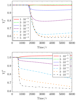
Figure 18: $Y_{2}^{P}$ as defined in Eq. (30) vs. time (in units of $\tau$) in vesicle systems (top: $\chi_{BS}=-0.15$) and droplet systems (bottom: $\chi_{BS}=0.75$) for different force amplitudes $f_{0}$ (units $f^{*}$) as indicated.

To analyze this effect, we introduce a quantity $Y_{2}^{P}$, which can be interpreted as the normalized variance of the polymer distribution in the direction perpendicular to the flow under the idealized assumption that the polymers are symmetrically distributed around $y=0$.

$$Y_{2}^{P}=\sqrt{\frac{\int_{-L_{y}/2}^{L_{y}/2}\mathrm{d}y\,y^{2}\Phi_{P}(y)}{\bar{\Phi}_{P}\int_{-L_{y}/2}^{L_{y}/2}\mathrm{d}y\,y^{2}}},$$ (30)

Here, $Y_{2}^{P}$ has been normalized such that a value of one corresponds to a uniform distribution, values above one correspond to situations where the polymeric matter preferably stays away from the center of the Poiseuille flow, and values below one indicate that the polymeric matter is focussed near the center. Results for the time evolution of this quantity are shown in 18. Both in vesicle and droplet systems, the polymeric matter is distributed uniformly across the systems in the initial stage prior to the first nucleation events. As nucleation sets in, $Y_{2}^{P}$ starts to deviate from unity.

We first examine the behavior for vesicle systems (18, top). For weak shear rates, $Y_{2}^{P}$ stays close to one at all times. For moderate shear rates, it drops down rapidly, until it reaches a shallow minimum. The level of the minimum decreases with increasing shear rates. Its position, $t\sim 2000-3000\tau$, roughly corresponds to the time where the vesicle fraction is largest according to 16, suggesting that the subsequent very slight increase of $Y_{2}^{P}$ is associated with the disruption of vesicles. Finally, at strong shear rates, $Y_{2}^{P}$ initially drops sharply and then saturates at a value around 0.6, which no longer depends on the strength of the shear force. In droplet systems (18, bottom), the initial drop of $Y_{2}^{P}$ at intermediate and strong shear rates is steeper than in the vesicle systems, almost instantaneous, and it ends in a sharp crossover to a second regime where $Y_{2}^{P}$ continues to decrease more slowly. A minimum is not encountered.

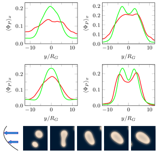
Figure 19: Polymer composition profile in $y$ direction for vesicle systems (green: $\chi_{BS}=-0.15$) and droplet systems (red: $\chi_{BS}=0.75$) at force amplitude $\mbox{$f_{0}$}=2\cdot 10^{-4}f^{*}$ (top) and $\mbox{$f_{0}$}=4\cdot 10^{-4}f^{*}$ (middle) shortly after the nucleation stage (left: $t=700\tau$ for droplet systems and $t=2200\tau$ for vesicle systems) and during the ripening stage (right: $t=6000\tau$). Bottom: Snapshots of a typical fusion process in a droplet system ($\chi_{BS}=0.75$) at $\mbox{$f_{0}$}=2\cdot 10^{-4}f^{*}$ and times $t=\{1500\tau,1900\tau,2800\tau,4000\tau,6000\tau\}$

19 shows actual monomer density profiles shortly after the nucleation stage (left) and at late times (right) for two different shear rates (top and bottom) both for vesicle and droplet systems (green and red lines). At a qualitative level, the behavior of vesicle and droplet systems is similar: Shortly after the nucleation stage, the profiles feature a single peak close to the center of the profile. At later times, a symmetric double peak structure emerges.

We will now discuss the origin of this twin peak structure in more detail. We first focus on the droplet systems. Here, the monomer density distribution at late times is governed by the interplay of ripening and particle fusions. The ripening is driven by the competition of bulk and surface energy, hence spherical particles at the center of the flow should grow at the expense of more elongated particles in the outskirts of the profile. This effect thus focusses matter to the center of the profile. However, it must be small, since the particle dissolution rate depends only weakly on the shear in the system according to 11. On the other hand, particle fusions typically drive matter away from the center of flow, as demonstrated in 19, bottom. As discussed in Sec. IV.2, shear enables fusion events. Hence the center of mass of two fusing particles will typically be located at a region of shear, $y\neq 0$, and the fusion event will drag matter to the periphery from the particle which is closer to the center.

In vesicle systems, the main mechanism responsible for the development of the characteristic twin-peak structure is the fingering instability which transforms the vesicles into rodlike particles as described in Sec. IV.3. This mechanism leads to a net transfer of polymeric matter from the vesicle in the flow maximum towards its ”fingers” outside the flow maximum. The alignment of the newly developed rods in the shear flow also contributes to the focussing of polymeric matter at some distance to the flow maximum.

The lateral drift and the equilibrium position of particles or droplets in Poiseuille flow has already been subject to many studies. In most of these studies, the droplets were introduced as a separate fluid, which did not mix with the solvent ^{56; 60; 54; 57} and had a conserved volume and in some cases even a conserved surface area. Therefore, hydrodynamic boundaries played an important role. Even more importantly, the systems under consideration also contained walls, which played a crucial role for the lateral migration behavior of the droplets.

In our example we deliberately eliminated the effect of walls and did not impose special hydrodynamic boundaries between particle and fluid. The particle is considered a part of the fluid, it has the same viscosity, and its only effect on the fluid dynamics is to impose surface forces generated by the solvent-particle interfaces. This allows us to extract the pure effect of the kinetics of self-assembly on the lateral distribution of particles. The observed lateral drifts are caused by the remodelling of polymeric matter, which is driven by the free energy landscape and guided by the non-local diffusive dynamics of the polymers. This kind of particle deformation and reformation of polymeric matter has already been observed before in simulations of polymer solutions or melts under shear flow ^{61; 62} or in nanotubes ⁶⁴.

V Discussion and Conclusions

The two main messages of the present paper can be summarized as follows:

First, we have presented a new mesoscale simulation method for polymer solutions, which couples a field-based dynamical model for diffusive polymer motion with a nonlocal mobility function accounting for the chain connectivity with a Lattice-Boltzmann scheme describing the hydrodynamic flows. It extends a method proposed previously by Zhang et al. ¹¹, which relied on a local dynamics assumption (monomers move independently). We have shown that the new model reproduces experimental observations such as the absence of vesicle fusions in closed systems. In previous simulations based on local dynamics ¹¹, fusions had been much too frequent.

The method allows us to study the dynamic evolution of inhomogeneous polymer systems on length scales in the range of $\sim$ 10 nanometers to micrometers and on time scales in the range of microseconds up to milliseconds. For example, in the present study, we can map the simulation units for length and time, $R_{G}$ and $\tau$, to real SI-units by mapping the radius of gyration of polymers (typically of order $R_{G}\sim 10\mbox{nm}$) and the diffusion constant of polymers in solution (typically of order $D_{p}\sim 10^{-6}\mbox{cm}^{2}/\mbox{s}$), giving the time unit $\tau=R_{G}^{2}/ND_{P}\sim 0.1\mu\mbox{s}$. Hence we simulated systems of size around $0.5$ micrometers over a time of around $0.5$ milliseconds.

Second, we have used our method to study the effect of shear flow on the self-assembly of droplets or vesicles after a sudden quench from a homogeneous copolymer solution. We have shown in Sec. IV that shear flow can be used to manipulate and control self-assembly in various ways. In the following we recapitulate and discuss mainly those aspects that may turn out relevant in particle design.

(i) Particle number and particle size.

Poiseuille flow was found to affect the final number of particles in two ways. First, shear flow increases the ”nucleation time”, i.e. , the characteristic time when the first nuclei emerge after the quench. During the narrow time window of the ”nucleation stage” (which ends when most copolymers from solution have been consumed), nucleation is therefore mostly restricted to the central low-shear part of the Poiseuille flow profile. As a result, fewer particles are nucleated in strong Poiseuille flow than in unsheared systems. A second effect of shear flow effect which further reduces the particle number at later times is the enhanced rate of particle fusions. Whereas particle fusions are almost fully suppressed in the absence of shear, they become possible and sometimes even dominate over particle dissolutions in the presence of shear. Hence sheared systems contain fewer particles than closed systems.

This has consequences for the size of the self-assembled particles. At given copolymer volume fraction, the average particle size is inversely proportional to the number of particles. Hence the average size of self-assembled particles should increase with the shear rate if self-assembly takes place in Poiseuille flow, due to the fact that fewer particles are nucleated and they merge more easily.

It should be noted that in reality, the size of nanoparticles that are assembled in microreactors is often found to decrease with increasing flow rate ⁹². The reason is that the quench rate in microreactor setups is gradual and coupled to the flow rate – for example, a microfluidic device may be used to mix a component into a (co)polymer solution, which induces (co)polymer aggregation. In such cases, the flow rate controls the particle size also via the quench rate ^{93; 85}, and as a result, particle sizes are smaller at larger flow rate.

Hence the influence of shear on the particle size depends on the experimental conditions. However, we can generally conclude that shear rates can be used to control the size of particles via a variety of (sometimes competing) mechanisms.

(ii) Shape transformations.

Under shear, both micelle-shaped droplets and vesicles elongate. The elongation disappears if the flow is stopped, and the particles become spherical again. However, irreversible shape changes were also observed. In particular, vesicles were found to develop fingering instabilities and to turn into rod micelles at late times. Such irreversible shape changes under shear could be used to design particle structures that cannot be assembled under equilibrium conditions.

(iii) Distribution of particles in Poiseuille flow.

We found that self-assembled particles tend to be distributed in a twin peak structure around the center of the Poiseuille flow profile. This can be used to design particle distributions through inhomogeneous shear flows.

Outlook.

It should be noted that all the results presented in the present paper were obtained in two dimensional simulations. Some of the results are presumably also valid in three dimensions. For example, we expect that the emergence of nuclei after a sudden quench is still delayed in the presence of shear, and that particle fusions are still facilitated by shear. In other respect, the scenario in three dimensions can be expected to be quite different. In particular, we can expect a much richer spectrum of irreversible shape transitions under shear. According to recent studies of vesicles in Poiseuille flow one might expect parachutes or, in case the vesicles are not in the flow maximum, slipper shapes ^{57; 56}. In strong shear flows it seems likely, that, according to ^{61; 62; 63; 64}, fingers will develop and lead to long rods as in two dimensions. Hence an extension of our study to three dimensions should be promising.

In real micro- and nanochannels, the presence of side walls also significantly affects both the self-assembly and the flow effects. The present study was deliberately set up to eliminate confinement effects and focus on the effect of a spatially varying shear flow. In reality, the interplay of flow and confinement should provide even more possibilities to design optimal flow geometries for nanoparticle synthesis. Mesoscale simulation methods such as the one proposed here should be useful to develop and assess such designs.

Appendix A Rotation of the force field

In this appendix, we show that the force field $\textbf{f}_{I}(\textbf{r})$ defined by Eq. (18) is indeed irrotational within the EPD approximation. Starting from Eq. (18), the rotation of the force field can be calculated according to

$$\nabla_{\textbf{r}}\times\textbf{f}_{I}(\textbf{r}) =-\nabla_{\textbf{r}}\times\sum_{J}\int\mathrm{d}\textbf{r}^{\prime}P_{IJ}(\textbf{r},\textbf{r}^{\prime})\nabla_{\textbf{r}^{\prime}}\mu_{J}(\textbf{r}^{\prime})$$

$$=\sum_{J}\int\mathrm{d}\textbf{r}^{\prime}\nabla_{\textbf{r}^{\prime}}P_{IJ}(\textbf{r},\textbf{r}^{\prime})\times\nabla_{\textbf{r}^{\prime}}\mu_{J}(\textbf{r}^{\prime})$$

Here, we have used the EPD approximation $\nabla_{\textbf{r}}P_{IJ}(\textbf{r},\textbf{r}^{\prime})=-\nabla_{\textbf{r}^{\prime}}P_{IJ}(\textbf{r},\textbf{r}^{\prime})$ ⁴⁰. From ⁹⁵ and ⁴⁰ we know the explicit form of the two-body correlator.

$$P_{IJ}(\textbf{r},\textbf{r}^{\prime})=\sum_{s,s^{\prime}}P_{ss^{\prime}}(\textbf{r},\textbf{r}^{\prime})\delta_{sI}^{K}\delta_{s^{\prime}J}^{K}$$

$$=\sum_{s,s^{\prime}}n\langle\delta(\textbf{r}-\textbf{R}_{s})\delta(\textbf{r}^{\prime}-\textbf{R}_{s^{\prime}})\rangle\delta_{sI}^{K}\delta_{s^{\prime}J}^{K}$$

$$=\sum_{s,s^{\prime}}n\int_{V^{N}}\mathrm{d}\textbf{R}_{1}...\mathrm{d}\textbf{R}_{N}\Psi\delta(\textbf{r}-\textbf{R}_{s})\delta(\textbf{r}^{\prime}-\textbf{R}_{s^{\prime}})\delta_{sI}^{K}\delta_{s^{\prime}J}^{K}$$

Here, $s$ and $s^{\prime}$ denote the index of the chain segment and $R_{s}$ is the position of monomer $s$ and $\psi$ the single chain distribution function. Hence we obtain

$$\nabla_{\textbf{r}}\times\textbf{f}_{I}(\textbf{r})$$

$$=\sum_{J}\epsilon_{ijk}\int\mathrm{d}\textbf{r}^{\prime}\big{(}\partial^{\prime}_{i}P_{IJ}(\textbf{r},\textbf{r}^{\prime})\big{)}\big{(}\partial^{\prime}_{j}\mu_{J}(\textbf{r}^{\prime})\big{)}\hat{\textbf{e}}_{k}\delta_{sI}^{K}\delta_{s^{\prime}J}^{K}$$

$$=\sum_{J}\epsilon_{ijk}\sum_{s,s^{\prime}}\int_{V^{N}}\mathrm{d}\textbf{R}_{1}...\mathrm{d}\textbf{R}_{N}\Psi\delta(\textbf{r}-\textbf{R}_{s})$$

$$\quad\times\int\mathrm{d}\textbf{r}^{\prime}\big{(}\partial^{\prime}_{i}\delta(\textbf{r}^{\prime}-\textbf{R}_{s^{\prime}})\big{)}\big{(}\partial^{\prime}_{j}\mu_{J}(\textbf{r}^{\prime})\big{)}\delta_{sI}^{K}\delta_{s^{\prime}J}^{K}\hat{\textbf{e}}_{k}$$

Now, we can apply partial integration to obtain

$$\nabla_{\textbf{r}}\times\textbf{f}_{I}(\textbf{r}) =-\sum_{J}\epsilon_{ijk}\sum_{s,s^{\prime}}\int_{V^{N}}\mathrm{d}\textbf{R}_{1}...\mathrm{d}\textbf{R}_{N}\Psi\delta(\textbf{r}-\textbf{R}_{s})$$

$$\quad\times\int\mathrm{d}\textbf{r}^{\prime}\delta(\textbf{r}^{\prime}-\textbf{R}_{s^{\prime}})\big{(}\partial^{\prime}_{i}\partial^{\prime}_{j}\mu_{J}(\textbf{r}^{\prime})\big{)}\delta_{sI}^{K}\delta_{s^{\prime}J}^{K}\hat{\textbf{e}}_{k}$$

$$=-\sum_{J}\int\mathrm{d}\textbf{r}^{\prime}\epsilon_{ijk}P_{IJ}(\textbf{r},\textbf{r}^{\prime})\big{(}\partial^{\prime}_{i}\partial^{\prime}_{j}\mu_{J}(\textbf{r}^{\prime})\big{)}$$

$$=-\sum_{J}\int\mathrm{d}\textbf{r}^{\prime}P_{IJ}(\textbf{r},\textbf{r}^{\prime})(\nabla\times\nabla\mu_{J}(\textbf{r}^{\prime}))=\textbf{0}$$

Appendix B Determination of the particle area

In Sec. IV.3 we introduced the particle area. Here, we explain briefly how it is determined from a composition distribution on a grid. First, we classify every lattice site with a polymer content of $\Phi_{P}\geq 0.5$ as a particle site. The contribution of particle sites to the total particle size depend on their local environment. Particle sites which are fully surrounded by particle sites count as one, the others count partially as illustrated in 20. We emphasize that the particle area describes the area covered by the polymers of the particle, and not its polymer content.

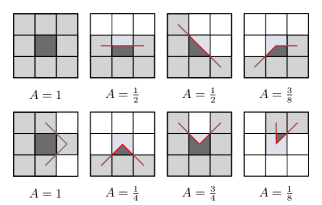
Figure 20: Weight factors $A$ with which a particle site (the central site) contributes to the total particle area for different local environments. Particle sites are shown in grey, ”empty” sites (with polymer content $\Phi_{P}<0.5$ are shown in white.

Appendix C Implementation of the simulation method

The simulation method combines two algorithms, which run in parallel and pass information to each other when ever needed. The work flow of the code is illustrated in the flow chart in 21. Here we use the short cut notation $\underline{\omega}$ and $\underline{\Phi}$ for the set of fields $\omega_{I},\Phi_{I}$ (with $I=A,B,S$), and $\underline{\underline{P}}$ for $P_{IJ}$. The operations (red boxes) are divided into an EPD and a LB column. The EPD column shows the evolution of the polymer-related fields $\underline{\Phi}$ and $\underline{\omega}$, and the LB column the evolution of the fluid-related fields $\rho$ (mass density) and $\mathbf{v}$ (fluid velocity). The dashed black lines show the work flow within each columns and mark the communication points. The blue boxes show the status of the fields at the beginning and end of a time step, and at selected intermediate states. The continuous red arrow indicates the serial processing of the single operations in our actual simulation program.

Four aspects in 21 need to be explained in more detail:

• ⁽¹⁾ The auxiliary convection step of $\omega$ is introduced in order to avoid a pinning of polymeric structures in cases where the fluid flow is so small that the changes of $\omega$ associated with the convection of $\Phi$ are below the accuracy threshold of the iteration loop ($10^{-8}$ in our simulations, see below).

• ⁽²⁾ $\tilde{\underline{\phi}}_{g}$ and the desired $\tilde{\underline{\phi}}$ are considered equal if $\sqrt{\frac{1}{V}\int\mathrm{d}\textbf{r}(\tilde{\underline{\phi}}-\tilde{\underline{\phi}}_{g})^{2}}<N_{tr}$, where $N_{tr}=1\cdot 10^{-8}$ in all simulation runs.

• ⁽³⁾ To estimate $\tilde{\underline{\omega}_{g}}$, the Fletcher-Reaves algorithm ⁷⁶ has been used.

• In the diffusion step, the current $\mathbf{j}^{D}$ is calculated from the $\delta F/\underline{\delta\Phi}$ as evaluated at the intermediate values of the composition field $\underline{\tilde{\phi}}$. Alternatively, one could also evaluate $\delta F/\underline{\delta\Phi}$ at the original values $\underline{\tilde{\phi}}(t)$. The resulting algorithm would have the same order (order one) as the present one. We have not compared the two algorithms. It will also be interesting to test more sophisticated, e.g., semi-implicit schemes.

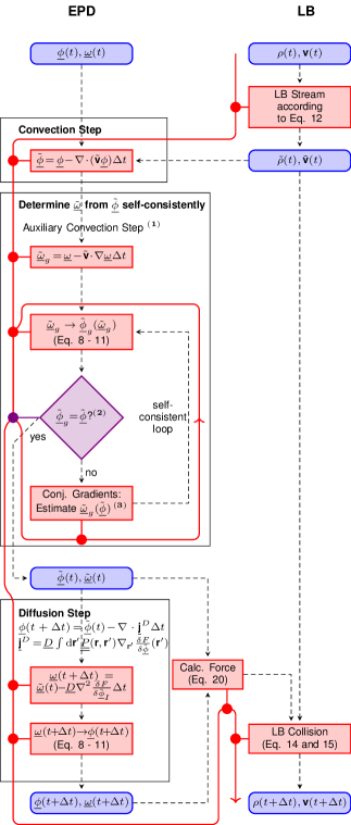
Figure 21: Flow chart diagram of the simulation program (one time step). See text for the comments (1,2,3) and for further explanation.

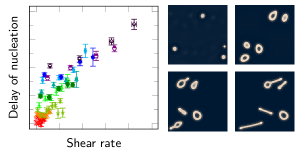
Figure 22: FOR TABLE OF CONTENTS ONLY. Title: Self-assembly of polymeric particles in Poiseuille flow: A hybrid Lattice Boltzmann / External Potential Dynamics simulation study. Authors: Johannes Heuser, G. J. Agur Sevink, Friederike Schmid

References

- Fredrickson (2013) Fredrickson, G. H. The Equilibrium Theory of Inhomogeneous Polymers; Oxford University Press: New York, 2013.
- Boudenne et al. (2011) Handbook of Multiphase Polymer Systems; Boudenne, A., Ibos, L., Candau, Y., Thomas, S., Eds.; Wiley, 2011.
- Bates and Fredrickson (1999) Bates, F. S.; Fredrickson, G. H. Physics Today 1999, 52, 32.
- Förster and Plantenberg (2002) Förster, S.; Plantenberg, T. Angew. Chemie Intnl. Ed. 2002, 41, 688–714.
- Schmid (2011) Schmid, F. Theory and simulation of multiphase polymer systems. In Handbook of Multiphase Polymer Systems; Boudenne, A., Ibos, L., Candau, Y., Thomas, S., Eds.; Wiley, 2011; Chapter 3, pp 31–80.
- Matsen and Schick (1994) Matsen, M. W.; Schick, M. Phys. Rev. Lett. 1994, 72, 2660.
- Matsen and Bates (1996) Matsen, M. W.; Bates, F. S. Macromolecules 1996, 29, 1091–1098.
- Tyler and Morse (2005) Tyler, C.; Morse, D. Phys. Rev. Lett. 2005, 94, 208302.
- Liu et al. (2016) Liu, M.; Qiang, Y.; Li, W.; Qiu, F.; Shi, A.-C. ACS Macro Lett. 2016, 5, 1167–1171.
- Arora et al. (2016) Arora, A.; Qian, J.; Morse, D. C.; Delaney, K. T.; Fredrickson, G. H.; Bates, F. S.; Dorfman, K. D. Macromolecules 2016, 49, 4675–4690.
- Zhang and Eisenberg (1995) Zhang, L.; Eisenberg, A. Science 1995, 268, 1728–1731.
- Antonietti and Förster (2003) Antonietti, M.; Förster, S. Adv. Mater. 2003, 15, 1323.
- Uneyama (2007) Uneyama, T. J. Chem. Phys. 2007, 126, 114902.
- He and Schmid (2008) He, X.; Schmid, F. Phys. Rev. Lett. 2008, 100, 137802.
- Zhang et al. (2011) Zhang, L.; Sevink, A.; Schmid, F. Macromolecules 2011, 44, 9434–9447.
- Seifert (1997) Seifert, U. Adv. in Phys. 1997, 46, 13–137.
- Discher and Eisenberg (2002) Discher, D. E.; Eisenberg, A. Science 2002, 297, 967–973.
- Langner and Sevink (2012) Langner, K. M.; Sevink, G. J. A. Soft Matter 2012, 8, 5102.
- de Vries et al. (2004) de Vries, A. H.; Mark, A. E.; Marrink, S. J. J. Am. Chem. Soc. 2004, 126, 4488–4489.
- Marrink and Mark (2003) Marrink, S. J.; Mark, A. E. J. Am. Chem. Soc. 2003, 125, 15233–15242.
- Noguchi and Takasu (2001) Noguchi, H.; Takasu, M. Phys. Rev. E 2001, 64, 041913.
- Noguchi and Takasu (2001) Noguchi, H.; Takasu, M. J. Chem. Phys. 2001, 115, 9547.
- Sevink et al. (2013) Sevink, G. J. A.; Charlaganov, M.; Fraaije, J. G. E. M. Soft matter 2013, 9, 2816–2831.
- Bernardes (1996) Bernardes, A. T. Langmuir 1996, 12, 5763–5767.
- Bernardes (1996) Bernardes, A. T. J. Phys. II 1996, 6, 169.
- Huang et al. (2009) Huang, J.; Wang, Y.; Qian, C. J. Chem. Phys. 2009, 131, 234902.
- Han et al. (2010) Han, Y.; Yu, H.; Du, H.; Jiang, W. J. Am. Chem. Soc. 2010, 132, 1144–1150.
- Han et al. (2012) Han, Y.; Cui, J.; Jiang, W. J. Phys. Chem. B 2012, 116, 9208–9214.
- Yamamoto et al. (2002) Yamamoto, S.; Maruyama, Y.; Hyodo, S.-A. J. Chem. Phys. 2002, 116, 5842–5849.
- Sevink et al. (2017) Sevink, G. J. A.; Schmid, F.; Kawakatsu, T.; Milano, G. Soft Matter 2017, 13, 1594–1623.
- Ortiz et al. (2005) Ortiz, V.; Nielsen, S. O.; Discher, D. E.; Klein, M. L.; Lipowsky, R.; Shillcock, J. J. Phys. Chem. B 2005, 109, 17708–17714.
- He et al. (2010) He, P.; Li, X.; Kou, D.; Deng, M.; Liang, H. J. Chem. Phys. 2010, 132, 204905.
- Xiao et al. (2012) Xiao, M.; Xia, G.; Wang, R.; Xie, D. Soft matter 2012, 8, 7865–7874.
- Guo et al. (2013) Guo, Y.; Ma, Z.; Ding, Z.; Li, R. K. Y. Langmuir 2013, 29, 12811–12817.
- Freed (1995) Freed, K. J. Chem. Phys. 1995, 103, 3230–3239.
- Uneyama and Doi (2005) Uneyama, T.; Doi, M. Macromolecules 2005, 38, 196.
- Schmid (1998) Schmid, F. J. Phys.: Condens. Matter 1998, 10, 8105–8138.
- Matsen (2002) Matsen, M. W. J. Phys.: Cond. Matter 2002, 14, R21–R47.
- Fraaije (1993) Fraaije, J. G. E. M. J. Chem. Phys. 1993, 99, 9202.
- Maurits and Fraaije (1997) Maurits, N. M.; Fraaije, J. G. E. M. J. Chem. Phys. 1997, 107, 5879–5889.
- Müller and Schmid (2005) Müller, M.; Schmid, F. Advances in Polymer Science 2005, 185, 1–58.
- Honda and Kawakatsu (2008) Honda, T.; Kawakatsu, T. J. Chem. Phys. 2008, 129, 114904.
- Sevink and Zvelindovsky (2005) Sevink, G. J. A.; Zvelindovsky, A. V. M. Macromolecules 2005, 38, 7502.
- Sevink and Zvelindovsky (2007) Sevink, G. J. A.; Zvelindovsky, A. V. M. Mol. Sim. 2007, 33, 405–415.
- He et al. (2004) He, X.; Liang, H.; Huang, L.; Pan, C. J. Phys. Chem. B 2004, 108, 1731–1735.
- He and Schmid (2006) He, X.; Schmid, F. Macromolecules 2006, 39, 2654–2662.
- He and Schmid (2006) He, X.; Schmid, F. Macromolecules 2006, 39, 8908–8910.
- Rallison (1984) Rallison, J. M. Ann. Rev. Fluid Mech. 1984, 16, 45.
- Kraus et al. (1996) Kraus, M.; Wintz, W.; Seifert, U.; Lipowsky, R. Phys. Rev. Lett. 1996, 77, 3685.
- Guido and Preziosi (2010) Guido, S.; Preziosi, V. Adv. Colloid Interface Sci. 2010, 161, 89–101.
- Vananroye et al. (2008) Vananroye, A.; Janssen, P. J. A.; Anderson, P. D.; Puyvelde, P. V.; Moldenaers, P. Phys. Fluids 2008, 20, 013101.
- Noguchi and Gompper (2005) Noguchi, H.; Gompper, G. Proc. Natl. Acad. Sci. USA 2005, 102, 14159–14164.
- Coupier et al. (2012) Coupier, G.; Farutin, A.; Minetti, C.; Podgorski, T.; Misbah, C. Phys. Rev. Lett. 2012, 108, 178106.
- Doddi and Bagchi (2008) Doddi, S. K.; Bagchi, P. International Journal of Multiphase Flow 2008, 34, 966.
- Mendes et al. (1997) Mendes, E.; Narayanan, J.; Oda, R.; Kern, F.; Candau, S. J.; Manohar, C. J. Phys. Chem. B 1997, 101, 2256–2258.
- Kaoui et al. (2008) Kaoui, B.; Ristow, G. H.; Cantat, I.; Misbah, C.; Zimmermann, W. Phys. Rev. E 2008, 77, 021903.
- Farutin and Misbah (2013) Farutin, A.; Misbah, C. Phys. Rev. Lett. 2013, 110, 108104.
- Segre and Silberberg (1961) Segre, G.; Silberberg, A. Nature 1961, 189, 209.
- Farutin and Misbah (2014) Farutin, A.; Misbah, C. Phys. Rev. E 2014, 89, 042709.
- Mortazavi and Tryggvason (2000) Mortazavi, S.; Tryggvason, G. J. Fluid Mech. 2000, 411, 325.
- Zvelindovsky et al. (1998) Zvelindovsky, A. V. M.; van Vlimmeren, B. A. C.; Sevink, G. J. A.; Maurits, N. M.; Fraaije, J. G. E. M. J. Chem. Phys. 1998, 109, 8751.
- Zvelindovsky and Sevink (2003) Zvelindovsky, A. V. M.; Sevink, G. J. A. Europhys. Lett. 2003, 62, 370.
- J. Cui and W. Li (2011) J. Cui, Z. M.; W. Li, W. J. Chem. Phys. 2011, 386, 81.
- Feng et al. (2008) Feng, J.; Liu, H.; Hu, Y.; Jiang, J. Macromol. Theory Simul. 2008, 17, 163.
- Tanaka (2005) Tanaka, H. J. Phys.: Cond. Matt 2005, 17, S2795–S2803.
- Groot et al. (1999) Groot, R. D.; Madden, T. J.; Tildesley, D. J. Chem. Phys. 1999, 110, 9739.
- Noguchi and Gompper (2006) Noguchi, H.; Gompper, G. J. Chem. Phys. 2006, 125, 164908.
- Succi (2001) Succi, S. The Lattice Boltzmann Equation for Fluid Dynamics and Beyond; Oxford University Press: New York, 2001.
- Weiss et al. (2008) Weiss, T. M.; Narayanan, T.; Gradzielski, M. Langmuir 2008, 24, 3759–3766.
- Adams et al. (2008) Adams, D. J.; Adams, S.; Atkins, D.; Butler, M. F.; Furzeland, S. J. Contr. Release 2008, 128, 165–170.
- Gummel et al. (2011) Gummel, J.; Sztucki, M.; Narayanan, T.; Gradzielski, M. Soft matter 2011, 7, 5731–5738.
- Qian et al. (2012) Qian, H.; Yao, W.; Yu, S.; Chen, Y.; Wu, W.; Jiang, X. Chemistry-An Asian Journal 2012, 7, 1875–1880.
- Doi and Onuki (1992) Doi, M.; Onuki, A. Journal De Physique II 1992, 2, 1631–1656.
- E. Reister (2001) E. Reister, K. B., M. Müller Phys. Rev. E 2001, 64, 041804.
- Tzeremes et al. (2002) Tzeremes, G.; Rasmussen, K. O.; Lookman, T.; Saxena, A. Phys. Rev. E 2002, 65, 041806.
- Fletcher and Reeves (1964) Fletcher, R.; Reeves, C. M. The Computer Journal 1964, 7, 149–154.
- Gross et al. (2010) Gross, M.; Adhikari, R.; Cates, M.; Varnik, F. Phys. Rev. E 2010, 82, 056714.
- d’Humières et al. (2002) d’Humières, D.; Ginzburg, I.; Krafczyk, M.; Lallemand, P.; Luo, L.-S. Phil. Trans. R. Soc. Lond. A 2002, 360, 437–451.
- Dünweg and Ladd (2009) Dünweg, B.; Ladd, A. J. C. Advances in Polymer Science 2009, 221, 89–166.
- Dünweg et al. (2007) Dünweg, B.; Schiller, U.; Ladd, A. J. C. Phys. Rev. E 2007, 76, 036704.
- Maurits et al. (1998) Maurits, N. M.; Zvelindovsky, A. V.; Sevink, G. J. A.; van Vlimmeren, B. A. C.; Fraaije, J. G. E. M. J. Chem. Phys. 1998, 108, 9150–9154.
- Backer et al. (2005) Backer, J. A.; Lowe, C. P.; Hoefsloot, H. C. J.; Iedema, P. D. J. Chem. Phys. 2005, 122, 154503.
- Fedosov et al. (2010) Fedosov, D. A.; Karniadakis, G. E.; Caswell, B. J. Chem. Phys. 2010, 132, 144103.
- Smith et al. (1999) Smith, D. E.; Babcock, H. P.; Chu, S. Science 1999, 283, 1724–1727.
- Keßler et al. (2005) Keßler, S.; Schmid, F.; Drese, K. Soft Matter 2005, 12, 7231.
- Takebe et al. (1989) Takebe, T.; Sawaoka, R.; Hashimoto, T. J. Chem. Phys. 1989, 91, 4369–4379.
- Takebe et al. (1990) Takebe, T.; Fujioka, K.; Sawaoka, R.; Hashimoto, T. J. Chem. Phys. 1990, 93, 5271–5280.
- Hashimoto et al. (1993) Hashimoto, T.; Takebe, T.; Asakawa, K. Physica A 1993, 194, 338–351.
- J. W. Cahn (1958) J. W. Cahn, J. E. H. J. Chem. Phys. 1958, 28, 258–267.
- Theodorou and Suter (1985) Theodorou, D. N.; Suter, U. W. Macromolecules 1985, 18, 1206–1214.
- Taylor (1932) Taylor, G. I. Proc. R. Soc. London, Ser. A 1932, 138, 41.
- Thiermann et al. (2012) Thiermann, R.; Müller, W.; Montesions-Castellanos, A.; Metzke, D.; Löb, P.; Hessel, V.; Maskos, M. Polymer 2012, 53, 2205–2210.
- Nikoubashman et al. (2016) Nikoubashman, A.; Lee, V. E.; Sosa, C.; Prud’homme, R. K.; Priestley, R. D.; Panagiotopoulos, A. Z. ACS Nano 2016, 10, 1425–1433.
- Wagner (2016) Wagner, A. Graphical User Interface, https://www.ndsu.edu/pubweb/~carswagn/GUI/index.html, 2016, accessed 2016-12-02.
- Kawasaki and Sekimoto (1988) Kawasaki, K.; Sekimoto, K. Physica 1988, 148A, 361–413.