Simulating Copolymeric Nanoparticle Assembly in the Co-solvent Method: How Mixing Rates Control Final Particle Sizes and Morphologies

Abstract

The self-assembly of copolymeric vesicles and micelles in micromixers is studied by External Potential Dynamics (EPD) simulations – a dynamic density functional approach that explicitly accounts for the polymer architecture both at the level of thermodynamics and dynamics. Specifically, we focus on the co-solvent method, where nanoparticle precipitation is triggered by mixing a poor co-solvent into a homogeneous copolymer solution in a micromixer. Experimentally, it has been reported that the flow rate in the micromixers influences the size of the resulting particles as well as their morphology: At small flow rates, vesicles dominate; with increasing flow rate, more and more micelles form, and the size of the particles decreases. Our simulation model is based on the assumption that the flow rate mainly sets the rate of mixing of solvent and co-solvent. The simulations reproduce the experimental observations at an almost quantitative level and provide insight into the underlying physical mechanisms: First, they confirm an earlier conjecture according to which the size control takes place in the earliest stage of the particle self-assembly, during the spinodal decomposition of polymers and solvent. Second, they reveal a crossover between different morphological regimes as a function of mixing rate. Hence they demonstrate that varying the mixing rate in a co-solvent setup is an effective way to control two key properties of drug delivery systems, their mean size and their morphology.

I INTRODUCTION

Nanoparticles are molecule aggregates with spatial extensions on scales of $\sim$ 10 to 100 nm. They have attracted growing interest during the last decades due to improved technologies for visualization and manipulation of nanoscale structures that have revealed their great potential for a wide range of applications. Depending on the chemical composition of the nanoparticles, these applications include mesoscopic models for atomic systems Herlach.2010 ; Smallenburg.2011 , optoelectronic devices Bucaro.2009 , nanoreactors, models for biological cells Lensen.2008 ; Discher.2002 , and most prominently, transport vehicles for medication, i.e. drug delivery systems Zhang.2008 ; Gindy.2009 ; Vartholomeos.2011 .

Most commercially available drug delivery systems are liposomes Allen.2004 ; Bleul.2014 , which are vesicular particles made of amphiphilic lipids. Biocompatible amphiphilic (diblock) copolymers represent promising alternatives to the lipids, since they are more stable and can be synthesized and modified more easily Discher.1999 ; Thiermann.2014 ; Thiermann.2012 . In analogy to their lipid counterparts, vesicles built from amphiphilic diblock-copolymers are often called polymersomes Discher.1999 . In the context of drug delivery systems one key property of nanoparticles is their size, since it not only determines their loading capacity, but also the composition of their protein corona in blood Tenzer.2011 , which in turn affects retention times in the circulatory system. In addition, the nanoparticle size plays a critical role in passive targeting of tumors based on the Enhanced Permeability and Retention effect Maeda.2000 .

A method to manufacture nanoparticle populations with a specific mean size is the co-solvent method, also known as flash nanoprecipitation Zhang.2012 . In this method, an initial solution containing the molecular constituents of the nanoparticles (e.g., the copolymers) in good solvent is mixed with a selective or bad solvent. The mixing eventually triggers the precipitation of the constituents and the aggregation to particles. One way to tune the sizes of the particles is to vary the rate of solvent mixing Mueller.2009 ; Thiermann.2012 ; Thiermann.2014 ; Nikoubashman.2016 . In experiments, solvent mixing is often implemented by continuous flow mixing devices, called passive micromixers Mueller.2009 ; Thiermann.2012 ; Thiermann.2014 ; Nikoubashman.2016 . Mixing rates in passive micromixers increase with increasing flow rates $v$ Falk.2010 ; Drese.2004 ; Schonfeld.2004.2 , and in turn, particle sizes are found to decrease with increasing $v$. Thiermann et al. Thiermann.2012 ; Thiermann.2014 have recently carried out an extensive study on the relation between flow rates and particle size in such a micromixer setup. The constituents of their nanoparticles were amphiphilic diblock-copolymers with a hydrophobic polybutadiene block and a hydrophilic polyethylene-oxide block, and they used tetrahydrofuran as good solvent and water as selective co-solvent. They found that variations of $v$ for symmetric flow conditions in passive micromixers enable a reproducible control over the mean size $R$ of a particle population with relatively low polydispersity. The experimental data for $R$ could be described reasonably well by scaling laws $R\propto v^{\alpha}$, where the exponent $\alpha$ differs from measurement to measurement, but scatters around a mean value of $\alpha=-0.158$ with a standard deviation $\sigma_{\alpha}=0.058$ simon_diss .

In a recent publication we proposed an explanation for the experimentally observed nanoparticle size dependence on flow rates or equivalently, mixing times meinArtikel1 . We combined a simple Cahn-Hilliard equation with a Flory-Huggins-de Gennes free energy functional for homopolymers and implemented solvent mixing by a time dependent interaction parameter. The simulation results for the size of homopolymer aggregates at the (relatively well-defined) crossover between spinodal decomposition and subsequent coarsening were in good semiquantitative agreement with the experimentally determined sizes for stabilized copolymer particles from Thiermann et al Thiermann.2012 ; Thiermann.2014 (apart from a factor of two). This lead us to hypothesize that particle sizes in the co-solvent method are determined during the very early stages of phase separation. The description also provided an explanation for the typical scaling laws observed in experiments and predicted an analytical expression, $R\sim v^{-\alpha}$ with the exponent $\alpha=1/6$, which is in good agreement with the experimentally observed exponents. According to this theory, the particle sizes at different $v$ result from a competition of the repulsion between solvent molecules and monomers of the solvent-phobic block with the interfacial tension of diffuse interfaces in the very early stages of phase separation, during spinodal decomposition. With respect to the entire particle growth process the description in terms of the Cahn-Hilliard model is, however, incomplete. The Flory-Huggins-de Gennes free energy functional for homopolymers can only be applied in the early segregation regime, it does not describe the internal reorganization of copolymers inside the particles at later stages. In particular, it does not include a mechanism that physically stabilizes particles of finite size, and cannot be used to describe particles with more complex morphologies as can be observed in copolymeric systems.

Amphiphilic molecules may form particles of different morphologies in solution, including spherical micelles or vesicles Discher.2002 . Apart from the size, particle morphology is another key property of drug delivery systems because it affects the loading possibilities. Spherical micelles consist of a hydrophobic core surrounded by a shell of hydrophilic blocks and they can only be loaded with hydrophobic substances. Vesicles allow both hydrophilic and hydrophobic loading, which makes them appealing canditates for multifunctional drug delivery systems: Hydrophilic substances can be enclosed in their solvent containing core, while the hydrophobic part of the bilayer shell can be loaded with hydrophobic substances. These loading possibilities are important because some therapeutic substances are hydrophilic and others hydrophobic. An example for a hydrophilic substance is the toxic anti-cancer drug camptothecin Wall.1966 . Hydrophilic materials are, for instance, the anti-cancer drug doxorubicin Torchilin.2005 or the dye pholoxine B, which can be used to trace particles in in vitro cell binding studies or studies on (hydrophilic) loading efficiencies WMueller.2011 . Although vesicles are more versatile when it comes to loading possibilities, micelles have the advantage that, due to their smaller size compared to vesicles, they may enable ways of cellular uptake that bypass the drug efflux mechanism of cancer cells in order to treat multiresistant cancer Bleul.2014 ; Kabanov.2002 .

The experiments by Thiermann et al. Thiermann.2012 ; Thiermann.2014 clearly show that the flow rates in micromixers also affect the morphologies of the resulting particles. At small flow rates, vesicles dominate, while at larger flow rates, micelles become more frequent. Motivated by these observations, we here present a numerical study of copolymer aggregation in a co-solvent setup for different mixing rates, using a dynamic density functional approach that explicitly accounts for the molecular architecture of copolymers. To this end, we implement time dependent interaction parameters into the established ’External Potential Dynamics” (EPD) model Maurits.1997b , which has been successfully used to study spontaneous self-assembly of amphiphilic diblock-copolymers to nanoparticles He.2006 ; He.2008 . We focus specifically on the effect of mixing rates on particle morphologies, and how the existence of different particle morphologies affects the typical scaling behavior $R\propto v^{\alpha}$.

The article is organized as follows. In section II we present the theoretical model. In section III we specify the input parameters used in the current article. The results and the discussion is presented in section IV, and the summary is given in V. In the A, we discuss technical issues and describe a novel integration scheme which was used to perform the simulations.

II THEORETICAL MODEL

We consider a solution of an amphiphilic AB-diblock copolymer P and a single solvent S in a volume $V$ at temperature $T$. To describe the phase separation dynamics we apply the EPD model Maurits.1997b ; Muller.2005 ; He.2006 , which is based on the free energy functional of the popular Self Consistent Field (SCF) Theory for polymers Edwards.1965 ; Schmid.1998 :

$$\begin{split}\frac{\beta\>F}{n}=&-f_{S}\ln\left(\frac{Q_{S}}{Vf_{S}}\right)-\frac{f_{P}}{N}\ln\left(\frac{Q_{P}N}{V\,f_{P}}\right)+\frac{1}{V}\int_{V}\Big{[}-\omega_{A}\phi_{A}\\ &-\omega_{B}\phi_{B}-\omega_{S}\phi_{S}+\chi_{AB}\phi_{A}\phi_{B}+\chi_{AS}\phi_{A}\phi_{S}\\ &+\chi_{BS}\phi_{B}\phi_{S}+\frac{\kappa_{H}}{2}\left(\phi_{A}+\phi_{B}+\phi_{S}-1\right)^{2}\Big{]}\,d\vec{r}.\end{split}$$ (1)

Here $f_{P}$ and $f_{S}$ are the mean polymer and solvent volume fractions, $N$ is the number of monomers per polymer chain, $\kappa_{H}$ a mean compressive modulus of the solution Schmid.1998 ; Helfand.1975 , $\chi_{ij}$ the Flory-Huggins interaction parameter between species $i$ and $j$, and $\beta=1/k_{B}T$ the Boltzmann factor. The fields $\omega_{i}$ for $i=A$, $B$, $S$ are potentials in units of $\beta^{-1}=k_{B}T$ that act on the respective monomer species $i$, and $\phi_{i}=\nicefrac{{\rho_{i}}}{{\rho_{0}}}$ with $\rho_{0}=\nicefrac{{n}}{{V}}$ are normalized number densities, where $n=n_{S}+Nn_{P}$ is the total number of monomers and solvent molecules in the system. $n_{S}$ is the number of solvent molecules and $n_{P}$ the number of polymer chains. $Q_{P}$ is the partition function of a polymer chain subject to $\omega_{A}$ and $\omega_{B}$, while $Q_{S}$ is the partition function of a single solvent molecule exposed to $\omega_{S}$. These single chain partition functions are given by

$$Q_{P}=\int_{V}g(\vec{r},1)\,d\vec{r}\text{ and }Q_{S}=\int_{V}e^{-\omega_{S}(\vec{r})}\,d\vec{r}.$$ (2)

$g(\vec{r},s)$ is the end-segment distribution function and describes the probability that one end of a polymer chain segment of length $s$ is located at position $\vec{r}$. It obeys the inhomogeneous diffusion equation

$$\frac{\partial g}{\partial s}(\vec{r},s)=\Delta g(\vec{r},s)-N\omega g(\vec{r},s)\text{ with }g(\vec{r},0)=1$$ (3)

Helfand.1972 ; Fredrickson.2006 , where omega is defined by

$$\omega=\begin{dcases*}\omega_{A}&$0<s<c_{A}$\\ \omega_{B}&$c_{A}<s<1$\\ \end{dcases*}.$$ (4)

$\vec{r}$ denotes the position in units of the polymer’s radius of gyration $R_{g}$, $s\in[0,1]$ represents the position along a polymer chain in units of $N$, and $c_{A}$ specifies the fraction of $A$-monomers in the diblock copolymer. If the polymer chain contains $N_{A}$ monomers of type $A$, one has $c_{A}=\nicefrac{{N_{A}}}{{N}}$. Since the potential fields in the SCF Theory mimic mean interactions between different species, they depend on the densities. Introducing a second distribution function $g^{\prime}$, which also solves equation (3) with

$$\omega=\begin{dcases*}\omega_{B}&$0<s<c_{B}$\\ \omega_{A}&$c_{B}<s<1$\\ \end{dcases*}$$ (5)

and $c_{B}=\nicefrac{{N_{B}}}{{N}}=1-c_{A}$, the relation between the potential fields $\omega_{i}$ and the densities $\phi_{i}$ from the SCF Theory can be cast into the form

$$\phi_{A}(\vec{r})[\omega_{A}]=\frac{Vf_{P}}{Q_{P}}\int_{0}^{c_{A}}g(\vec{r},s)g^{\prime}(\vec{r},1-s)\,ds,$$ (6)

$$\phi_{B}(\vec{r})[\omega_{B}]=\frac{Vf_{P}}{Q_{P}}\int_{c_{A}}^{1}g(\vec{r},s)g^{\prime}(\vec{r},1-s)\,ds,$$ (7)

and

$$\phi_{S}(\vec{r})[\omega_{S}]=\frac{Vf_{S}}{Q_{S}}e^{-\omega_{S}(\vec{r})}.$$ (8)

In the EPD formalism the dynamical equations for the potential fields are given by

$$\begin{split}\frac{\partial\omega_{i}}{\partial t}(\vec{r},t)=-D_{i}\Delta\left(\mu_{i}(\vec{r},t)+\eta_{i}(\vec{r},t)\right)\text{ with }i=A,B,S,\\ \mu_{i}(\vec{r})=\frac{1}{\rho_{0}}\frac{\delta\beta F}{\delta\phi_{i}(\vec{r})}\text{, and }D_{i}=\begin{dcases*}D_{P}=\frac{D_{0}}{N}&$i=A,B$\\ D_{S}=D_{0}&$i=S$\\ \end{dcases*},\end{split}$$ (9)

where $\eta_{i}$ is a random noise and $\frac{\delta\beta F}{\delta\phi_{i}}$ is the variational derivative of $\beta F$ with respect to $\phi_{i}$. Equation 9 is equivalent to the dynamical master equation for monomer densitiy fields derived by Kawasaki and Sekimoto Kawasaki.1987 with a non-local kinetic coupling in a copolymer solution. The EPD formalism dramatically reduces the computational cost of the non-local coupling model and was first introduced by Maurits and Fraaije Maurits.1997b . Taking into account the density-field relations from the SCF Theory and that $Q_{P}=Q_{P}[\omega_{A},\omega_{B}]$ as well as $Q_{S}=Q_{S}[\omega]$, the chemical potentials $\mu_{i}$ can be calculated as

$$\mu_{A}=\chi_{AB}\phi_{B}+\chi_{AS}\phi_{S}+\kappa_{H}\left(\phi_{A}+\phi_{B}+\phi_{S}-1\right)-\omega_{A},$$ (10)

$$\mu_{B}=\chi_{AB}\phi_{A}+\chi_{BS}\phi_{S}+\kappa_{H}(\phi_{A}+\phi_{B}+\phi_{S}-1)-\omega_{B},$$ (11)

$$\mu_{S}=\chi_{AS}\phi_{A}+\chi_{BS}\phi_{B}+\kappa_{H}(\phi_{A}+\phi_{B}+\phi_{S}-1)-\omega_{S}.$$ (12)

Equations 3, 6 – 8, and 9 constitute a SCF-EPD model that has been used to successfully study self-assembly of particles with various morphologies He.2006 ; He.2008 .

In our previous publication we have shown that spinodal decomposition under time-dependent quenches into the spinodal area reproduce experimental trends meinArtikel1 . Therefore, solvent mixing in the present work is described in a very similar manner. We model solvent mixing by a time dependent interaction parameter between the solvent and the B-block, which is from now on considered to be the solvent-phobic one. If not stated otherwise, its time dependence is linear and given by

$$\chi_{BS}(t)=\begin{dcases*}\chi_{BS}^{(0)}+s_{\chi}t,&$t\leq t_{max}$\\ \chi_{BS}^{(max)},&$t>t_{max}$\\ \end{dcases*}.$$ (13)

The cutoff time $t_{max}=\nicefrac{{\left(\chi_{BS}^{(max)}-\chi_{BS}^{(0)}\right)}}{{s_{\chi}}}$ can be interpreted as a mixing time, and the parameter

$$\chi_{BS}^{(0)}=\frac{1}{2Nc_{B}f_{P}}+\frac{1}{2c_{B}(1-f_{P})}+\chi_{AB}c_{A}-\chi_{AS}\frac{c_{A}}{c_{B}}$$ (14)

is the spinodal solvent-phobic interaction for which ${\partial^{2}F_{FH}}/{\partial f_{P}^{2}}=0$, where $F_{FH}$ is the Flory-Huggins approximation to $F$ from equation (1) He.2006 .

III SIMULATION SETUP

Simulations start from randomly perturbed homogeneous initial states. All simulation results are averaged over five simulation runs with different initial conditions. We consider a volume fraction $f_{P}=0.1$ of a model polymer with a solvent-philic block length $N_{A}=3$ and an incompatible solvent-phobic block containing $N_{B}=14$ monomers. The incompatibility is described by an interaction parameter $\chi_{AB}=1.05$, and to keep $\phi_{A}+\phi_{B}+\phi_{S}$ close to 1, the compressive modulus is set to $\kappa_{H}=100$. The mean volume fraction of selective solvent is $f_{S}=1-f_{P}=0.9$. The diffusion coefficient $D_{0}$ in equation (9) can be substituted by $1$ without loss of generality as lengths are given in units of $l_{0}=R_{g}$ and times in units of $t_{0}=\nicefrac{{R_{g}^{2}}}{{D_{0}}}$. The solvent-philic interaction is kept at a constant value $\chi_{AS}=-0.15$, and the solvent-phobic one is varied from its spinodal value $\chi_{BS}^{(0)}=\chi_{BS}^{(Spin)}=1.249$ to $\chi_{BS}^{(max)}=2.25$, which corresponds to a maximum quench depth of approximately 1 like in reference meinArtikel1 . As in reference meinArtikel1 , the random noise is turned off, i.e. $\eta_{i}=0$.

The number of spatial grid points is set to $m=256\times 256$ with a lattice constant $\Delta l=0.25R_{g}$. The time step $h$ varies during the simulation as described in A. Unless stated otherwise, we use an initial (and maximum) time step of $h=0.05t_{0}$. The segment length in a polymer chain is $ds=\nicefrac{{1}}{{N}}$. Simulations are restricted to two dimensions (2D) because the qualitative size dependence was shown to be independent of the dimension in meinArtikel1 . In 2D, much larger systems can be simulated over longer time periods.

The set of equations (3) and (6 – 8) is solved with the same solvers as in Ref. He.2006 . The evolution equations for the potential fields (9) is solved by a newly developed semi-implicit integration scheme, which is presented in A.

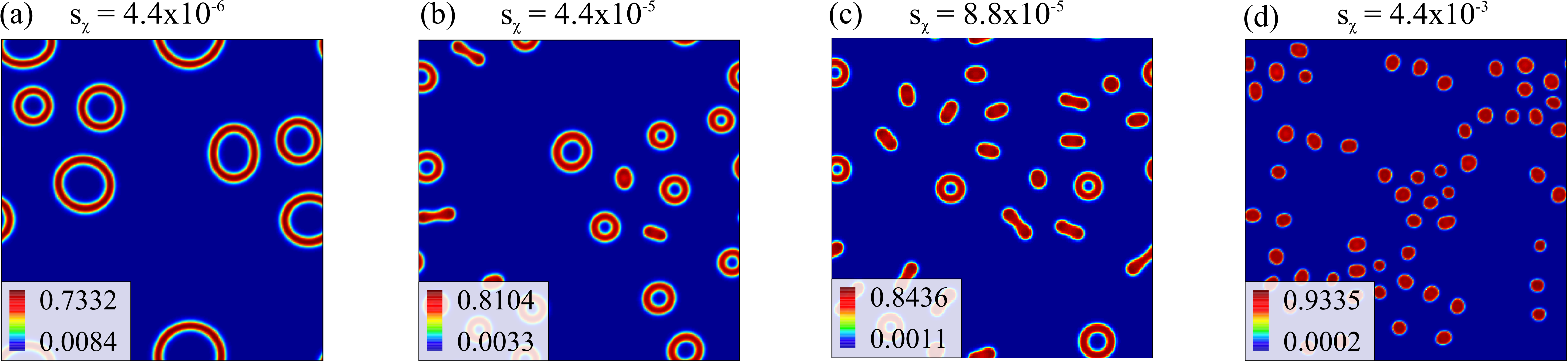
Figure 1: Color coded solvent-phobic density profiles $\phi_{B}$. (a) shows simulation results at a mixing rate of $s_{\chi}=4.4\times 10^{-6}$ (b) at $s_{\chi}=4.4\times 10^{-5}$, (c) at $s_{\chi}=8.8\times 10^{-5}$, and (d) at $s_{\chi}=4.4\times 10^{-3}$. An increase of mixing rates does not only affect particle sizes but also induces a morphological vesicle-to-micelle transition.

IV RESULTS AND DISCUSSION

IV.1 Morphological transition and qualitative discussion of particle size dependencies on mixing speeds

Figure 1 depicts simulated polymer particles for different mixing speeds $s_{\chi}$. Strictly speaking, only the density of solvent-phobic B-monomers $\phi_{B}$ is shown, but since the A-monomers accumulate approximately at green to yellow $\phi_{B}$-values, these colors can be imagined to represent the solvent-philic A-block. It is evident that an increase of the mixing rate leads to a decrease of the typical particle size and induces a morphological vesicle-to-micelle transition: From figure 1 (a) to (d), the number of vesicles decreases while the number of micelles increases until only spherical micelles are left. For every $s_{\chi}$, the $\phi_{B}$-profiles in the early stages of phase separation (not shown) closely resemble the profiles obtained in our earlier work based on the Cahn-Hilliard equation for homopolymers meinArtikel1 . Once the polymer content inside polymer aggregates is sufficiently high, the block incompatibility leads to an internal rearrangement of copolymer chains inside the aggregates, which eventually leads to the formation of different morphologies. In the literature, different pathways of vesicle formation have been described theoretically and observed experimentally He.2006 ; Uneyama.2007 ; He.2008 ; weiss1 ; adams1 ; gummel1 . In the present simulations, they form by nucleation and growth (mechanism II according to Ref. He.2008 ). The solvent-philic A-block, ultimately oriented towards the solvent, sterically stabilizes the particles by suppressing further ripening (where large particles grow and smaller particles dissolve) and preventing macrophase separation He.2006 .

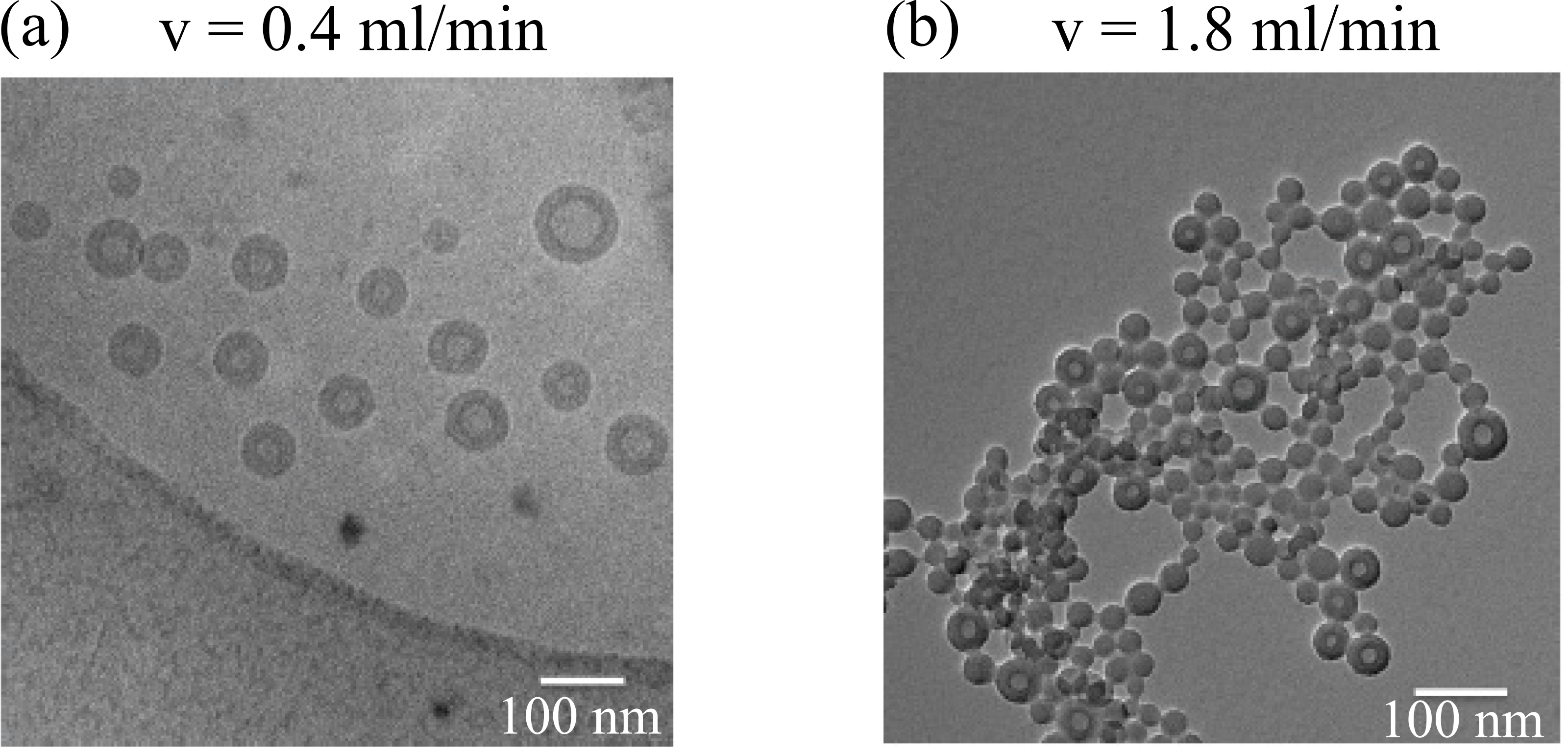
Figure 2: Transmission Electron Microscopy images of cross-linked nanoparticles made of polybutadiene-polythyleneoxide diblock copolymers obtained in the Caterpillar Micromixer at two different flow rates as indicated and otherwise identical experimental parameters under symmetric flow conditions. After Ref. Thiermann.2014 (samples Cd10 and Cd11), courtesy of R. Thiermann.

An enrichment of micelles with increasing flow rate comparable to figure 1 (a) to (c) is also observed experimentally. Transmission Electron Microscopy (TEM) images from experiments are shown in figure 2. Figure 2 (a) and (b) provide a direct comparison of identically prepared polymer solution samples for two different flow rates Thiermann.2014 in the Caterpillar Micromixer Schonfeld.2004.2 , i.e. for two different mixing rates. The particle morphologies resemble the simulation results from figure 1 (a) and (c), except that the TEM images lack cylindrical micelles while the simulation results contain a few. In other experimental work Mueller.2009 , such cylindrical micelles have also been found to coexist with spherical micelles and vesicles. Whether or not cylindrical micelles appear in simulations likely depends on the interaction parameters $\chi_{AB}$ and $\chi_{AS}$. We conclude that qualitatively, the dependence of morphologies on mixing rates is in good agreement with experiments. Furthermore, the simulations indicate that the enrichment of micelles only marks the onset of a complete morphological transition from vesicular to micellar.

IV.2 Minkowski measures and determination of particle sizes

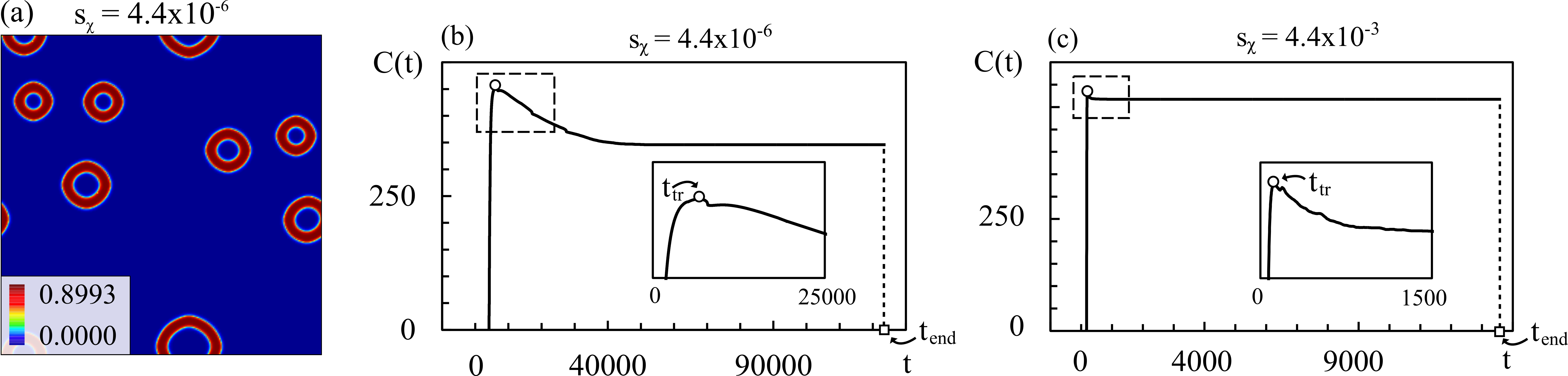
Figure 3: Vesicles at $t_{end}>t_{tr}$ (a) and time series of the Minkowski measure $C(t)$ for $s_{\chi}=4.4\times 10^{-6}$ (b) and $s_{\chi}=4.4\times 10^{-3}$ (c). The transition time $t_{tr}$ is labeled by a circle. $t_{end}$ denotes the end of a simulation run and is marked by a rectangle. The insets in (b) and (c) show a magnification of the respective part framed by the rectangle.

The snapshots in figure 1 are taken at the so-called transition time $t_{tr}$ Sofonea.1999 . In the Cahn-Hilliard model, the transition time separates a regime of spinodal decomposition and initial droplet nucleation and growth, where polymer aggregates form and concentrate, from a comparatively slow ripening regime, where small aggregates grow at the expense of smaller ones until only one single polymer aggregate remains. The transition time $t_{tr}$ can be determined by inspecting, for instance, the Minkowski measure $C$ Sofonea.1999 . Here $C$ denotes the total boundary length of the union over all subsets where $\phi_{B}$ exceeds a predefined threshold $\phi_{B}^{(th)}$. The rapid concentration of solvent-phobic monomers in the spinodal decomposition stage leads to a very fast temporal increase of $C$, while ripening is characterized by a slow but steady decrease of $C$. This opposite behavior leads to a clear maximum in $C(t)$, which marks the transition time. Time series of $C$ in the SCF-EPD copolymer model are shown in figure 3. They look very similar to the Cahn-Hilliard model in our earlier studies meinArtikel1 . We still find the distinct maximum that allows an analogous definition of the transition time $t_{tr}$. As in the Cahn-Hilliard model, the steep rise at $t<t_{tr}$ is caused by a rapid initial polymer aggregation, which is already associated with the formation of different morphologies (see figure 1). The subsequent slow decrease of $C(t)$ is not caused by Ostwald Ripening, but mainly by a shrinking of particles. In the simulations from figure 1, this shrinking is most pronounced at $s_{\chi}=4.4\times 10^{-6}$. To give an impression of the extent of the shrinking, figure 3 (a) shows the density profiles from figure 1 (a) at the end of the simulation run, $t=t_{end}$. The shrinking and the increase of $\phi_{B}$-values between $t_{tr}$ and $t_{end}$ is most likely caused by the increase of $\chi_{BS}$ during this time interval. Finally, $C(t)$reaches a plateau at late times (see figure 3 (b) and (c)). This is in contrast to the Cahn-Hilliard model, where $C(t)$ continues to decay at late times. The plateau corresponds to a state where multiple stabilized particles are present.

We measure particle sizes at transition time because the shrinking is not very pronounced, and because a maximum of $C$ can be defined more precisely than a plateau. To this end, pictures such as those shown in figure 1 are converted into binary images with a threshold value of $\phi_{B}^{(th)}$. Then a standard 4-connected-component image labeling algorithm Nielsen.2014 is used to count and isolate single particles. Afterwards, the area $A_{i}$ and circumference $U_{i}$ is determined for every single particle $i=1,...,p$ in a picture with the Minkowski functional algorithm from Mantz et al. Mantz.2008 . We define the sphere equivalent radius $R_{s,i}$ and the vesicle equivalent radius $R_{v,i}$ of particle $i$ by

$$R_{s,i}=\sqrt{\frac{A_{i}}{\pi}}\text{ and }R_{v,i}=\frac{A_{i}}{U_{i}}+\frac{U_{i}}{4\pi},$$ (15)

respectively. The vesicle equivalent radius is the outer radius of the spherical shell with area $A_{i}$ and total perimeter $U_{i}$. In case a spherical micelle is processed, $R_{s,i}$ and $R_{v,i}$ are equal to its radius $R$, which can be verified by insertion of $A_{i}=\pi R^{2}$ and $U_{i}=2\pi R$. Mean particle sizes are estimated by the mean values

$$R_{s}=\frac{1}{p}\sum_{i=1}^{p}R_{s,i}\text{ and }R_{v}=\frac{1}{p}\sum_{i=1}^{p}R_{v,i}.$$ (16)

As a measure for polydispersity of a nanoparticle population we use the standard deviation

$$\Delta R_{j}=\sqrt{\frac{1}{p}\sum_{i=1}^{p}\left(R_{j}-R_{j,i}\right)^{2}}.$$ (17)

for $j=s,v$.

IV.3 Simulation results for particle sizes and morphological regimes

Figure 4 shows simulation results for particle sizes and transition times. Particle sizes are given in units of the polymer’s radius of gyration $l_{0}=R_{g}$ and times in units of $t_{0}=\nicefrac{{R_{g}^{2}}}{{D_{0}}}$. The dependence of particle sizes and transition times on quench rates also resembles the results from the Cahn-Hilliard model for homopolymers: There is an asymptotic regime, where particle sizes converge to results for a constant quench depth $\chi_{BS}(t)\equiv\chi_{BS}^{(max)}$, and there is a non-asymptotic regime, where particle sizes follow scaling laws $R\propto s_{\chi}^{\alpha}$ with $\alpha\approx-\nicefrac{{1}}{{6}}$, while transition times can be approximated by $t_{tr}\propto s_{\chi}^{-\nicefrac{{2}}{{3}}}$ meinArtikel1 . As in reference meinArtikel1 , the asymptotic and the non-asymptotic regime are separated by the time when $t_{max}$ in figure 4 intersects $t_{tr}$. The similarity of the data curves in figure 4 to our earlier Cahn-Hilliard results for homopolymers meinArtikel1 confirms the hypothesis that particle sizes are determined during the very early stages of phase separation, where the specific sequence of polymers (block copolymers vs. homopolymers) is not yet important. In particular, the predictions of the simple Cahn-Hilliard model meinArtikel1 can still be applied.

For diblock-copolymers, however, the non-asymptotic regime splits into three different morphological regimes. We call a morphological regime an interval of mixing rates with specific predominant particle morphologies. In figure 4 (a) the morphological regimes are separated by the vertical lines. At low mixing rates only vesicles form. Figure 1 (a) shows a corresponding snapshot of particles. At intermediate mixing rates one gets a mixture of vesicles, cylindrical micelles and spherical micelles. In the intermediate regime the number of vesicles decreases with increasing mixing rates while the number of micelles increases. Corresponding snapshots of particles can be found in figure 1 (b) and (c). At large mixing rates there are only micelles as seen in figure 1 (d). Because every morphological regime covers a certain interval of particle sizes, particle morphologies are directly coupled to their size. With respect to the co-solvent method this means that it should be possible to produce pure vesicular or micellar populations at ’extremely’ large or low flow rates, but intermediate ones typically result in heterogeneous morphologies. As long as the micelles are not exclusively spherical, $R_{v}$ is larger than $R_{s}$ because the formation of vesicles from a polymer aggregate increases the perimeter $U_{i}$ of a spherical shell, while it keeps the volume $A_{i}$ constant.

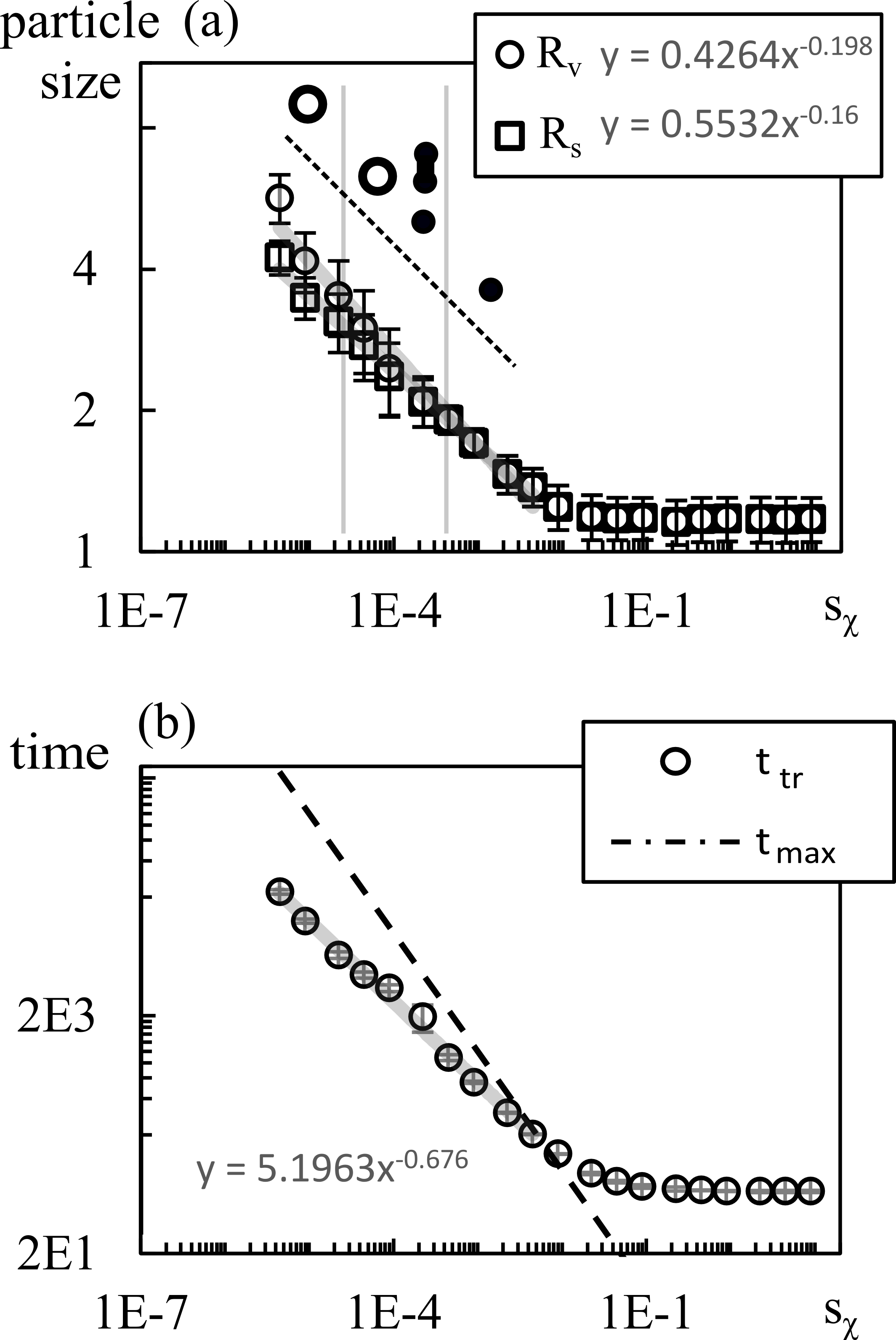
Figure 4: Simulation results for particle sizes (a) and transition times (b) in dependence on the quench rate $s_{\chi}$. The data points in (a) represent the simulation results for the sphere and vesicle equivalent radius from equation (16) and the error bars are the standard deviation from equation (17). Trend line equations are given in the legend. The vertical lines separate three different morphological regimes, where the corresponding morphologies above the dashed line appear. Empty circles symbolize vesicles, solid black dots spherical micelles and the dumbbell cylindrical micelles. The data points in (b) are the transition times $t_{tr}$ (cp. figure 3) and the dashed line is $t_{max}$ from equation (13). The trend line equation refers to the transition time. Error bars are standard deviations over five different simulation runs.

It should be noted though that the simulated ”micelles” from the rightmost morphological regime in figure 4 (a) are, strictly speaking, actually no ’real’ micelles. Real micelles are equilibrium structures with a well-defined size distribution and composition that does not depend on the history of the system. Here, we consider ’micelle-like’ spheres with the typical core-shell structure that would be characteristic for a micelle, but they are not equilibrated.

IV.4 Comparison of particle sizes to experimental results

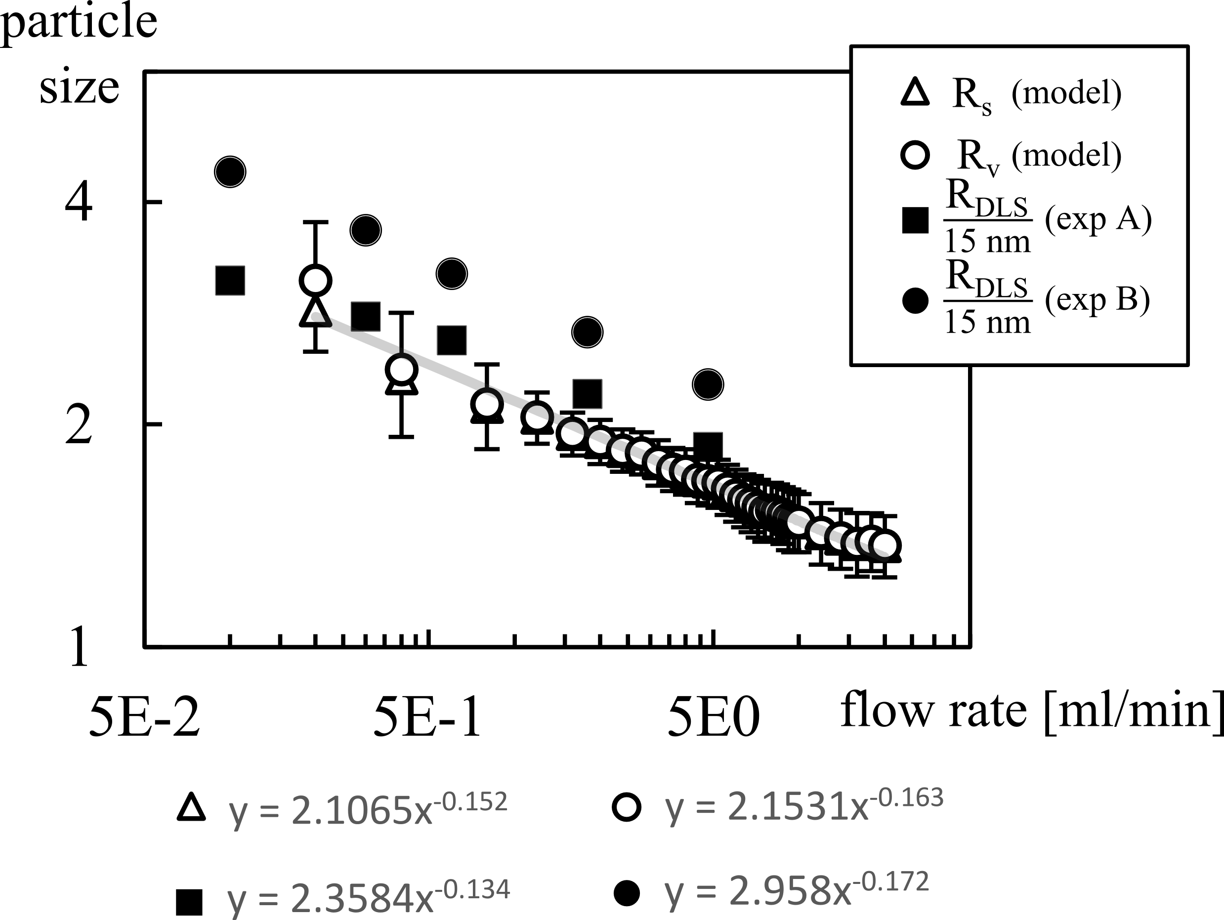
Figure 5: Particle sizes in units of $R_{g}$ versus flow rates $v$ in ml/min in the Caterpillar Micromixer. The open symbols represent simulation results and the solid symbols experimental results from Thiermann et al. Thiermann.2012 . A ($\hat{=}$ H) and B ($\hat{=}\text{CO}\text{--CH}_{2}\text{--CH}_{2}\text{--COOH}$ ) denote different end groups attached to the polymer. Trend line equations are shown beneath the diagram at the corresponding symbols. For the sake of simplicity only the regression line to $R_{s}$ is shown (thick light grey line). Error bars mark the polydispersity as determined from Eq. 17 and are again only shown for $R_{s}$ for the sake of clarity. $\Delta R_{v}$ looks very similar.

After having studied the idealized situation where the solvent mixing is described by the simple linear increase of $\chi_{BS}(t)$ with time, (Eq. (13)), we will now introduce a more general Ansatz which allows us to compare simulation results directly to experiments: We assume that $\chi_{BS}(t)$ is a linear function of the volume fraction of selective solvent $\varphi_{SS}(t)$, which we take to be homogeneous throughout the system. Specifically, we assume

$$\chi_{BS}(t)=\chi_{BGS}+\frac{\chi_{BSS}-\chi_{BGS}}{1-f_{P}}\varphi_{SS}(t),$$ (18)

where $\chi_{BGS}$ is the interaction parameter between the B-monomers and the good solvent, while $\chi_{BSS}$ describes the interaction of the B-monomers and the selective solvent. The Ansatz ensures that $\chi_{BS}=\chi_{BGS}$ if no selective solvent is present and $\chi_{BS}=\chi_{BSS}$ if only selective solvent is present, i.e. if $\varphi_{SS}=1-f_{P}$.

We assume that $\varphi_{SS}(t)$ can be calculated independently of the particle self-assembly simply by considering the mixing of simple fluids in a given micromixer geometry. This Ansatz allows a direct coupling of mixer geometries and flow rates into the description of particle growth. Here we specifically consider the case of the Caterpillar Micromixer (CPMM), where analytical expressions for $\varphi_{SS}(t)$ have been derived by Schoenfeld et al. Schonfeld.2004.2 . Simulation results for particle sizes with the mixing profile $\varphi_{SS}(t)$ from the Caterpillar micromixer are shown in figure 5. Even with this Ansatz, the data still show scaling behavior.

If we normalize the experimental data with 15 nm, i.e., we assume the gyration radius of the polymers to be around $R_{g}=$15 nm, we get almost quantitative agreement between simulation data and experiments. In reality, the radius of gyration is probably smaller, in the range of 5-10 nm meinArtikel1 ; simon_diss , hence the simulations probably underestimate the particle size. The simulations also reproduce the experimentally observed morphological transition from vesicles to micelles upon reducing the flow rate, but here again, the absolute values of flow rates where the morphological transition is observed in experiments and simulations do not match quantitatively. In the experiments pure vesicular populations are observed up to flow rates of approximately 1.8 ml/min, while in the simulations, micelles dominate already at flow rates above approximately 0.8 ml/min. The specific flow rate values of the vesicle to micelle transition as well as the final particle sizes are likely to depend strongly on $\chi_{AB}$ and $\chi_{AS}$. Since the material parameters of the experimental systems studied by Thiermann et al. Thiermann.2012 ; Thiermann.2014 were not determined, a direct quantitative comparison between model and experiments is difficult.

Nevertheless, our results show that the simulations reproduce the experimental trends and the order of magnitude of simulated particle sizes matches the experimentally observed sizes. This suggests that the main mechanism determining particle sizes is captured by our mean field model, even though it does not account for Brownian motion of particles and thereby induced collision induced coagulation and growth of particles.

To conclude, the results show that the combination of established methods for calculating solvent mixing in complex geometries on large scales with mean field theories for aggregation on mesoscales, coupled through an Ansatz like equation (18), represent a promising multiscale approach for describing flow controlled particle assembly in micromixers.

V SUMMARY AND OUTLOOK

We have implemented time dependent interaction parameters into a Dynamic Self Consistent Field Theory for copolymer simulations in order to describe the nonequilibrium assembly of amphiphilic diblock-copolymers in micromixers.

Experimental observations show that the final morphologies of particles are mostly vesicular at low mixing rates, and mostly micellar at high mixing rates Mueller.2009 ; Thiermann.2012 ; Thiermann.2014 . Our simulations indicate that these changes in morphologies are the signature of an incomplete vesicle-to-micelle transition, and that nanoparticle populations should be purely micellar if the flow rates are sufficiently large. We conclude that it should be possible to produce both pure vesicular and pure micellar nanoparticle populations with the co-solvent method. In the morphological regime at low flow rates, one can tune the size of vesicles, while in the regime at high flow rates the size of micelles can be adapted. The intermediate regime, however, excludes certain mean sizes if one wants to produce particles with only one morphology.

The rate of solvent mixing qualitatively affects particle sizes in the same way in the SCF-EPD model as in the Cahn Hilliard model for homopolymers. The present work hence confirms our conjecture in Ref. meinArtikel1 , that the sizes of particles that are aggregated from amphiphilic copolymer solutions are determined during the very early stages of phase separation by a competition between the interfacial tension of diffuse interfaces and the decreasing solvent quality for the solvent-phobic block. Furthermore, figure 4 shows that the rate-dependent morphological changes do not affect the typical scaling behavior $R\mathrel{\vbox{ \offinterlineskip\halign{\hfil$#$\cr\propto\cr\kern 2.0pt\cr\sim\cr\kern-2.0pt\cr}}}v^{-\nicefrac{{1}}{{6}}}$ in the non-asymptotic regime, which is observed here in copolymer solutions as well as in Ref. meinArtikel1 in homopolymer solutions.

As we have mentioned above, vesicles form via a nucleation-and-growth pathway in the simulations considered here (pathway II in Ref. He.2006 ), which is typical for the aggregation of particles from solutions with relatively low copolymer densities and/or relatively weak incompatibilities He.2008 . At higher copolymer concentrations He.2008 ; gummel1 , one observes an alternative aggregation-and-bending pathway (pathway I), where micellar particles first aggregate to platelets and these platelets then bend around, driven by a competition of bending energy and line tension, to form closed vesicles. In future work, it will be interesting to study the influence of the mixing rate on particle aggregation in the regime where pathway I is dominant. (These simulations would have to be done in three dimensions, since in two dimensions, the final step of platelet bending does not take place). In particular, it will be interesting to investigate whether the scaling law for the particle sizes, $R\mathrel{\vbox{ \offinterlineskip\halign{\hfil$#$\cr\propto\cr\kern 2.0pt\cr\sim\cr\kern-2.0pt\cr}}}s_{\chi}^{-\nicefrac{{1}}{{6}}}$, still persists in that regime. If the scaling law is destroyed, this would provide indirect evidence that the vesicle formation in the micromixers that have studied experimentally proceeds predominantly via mechanism II.

To implement mixer geometries into solvent mixing, we have coupled an established description for the Caterpillar Micromixer (CPMM) Schonfeld.2004.2 into the SCF-EPD model. Here, the interaction between the solvent and the solvent-phobic monomers was assumed to be a linear function of the volume fraction of selective solvent (cf. Eq. 18). This Ansatz allowed us to perform simulations of particle assembly with realistic mixing times and to compare directly the particle sizes obtained in experiments and simulations. The scale of the simulated particle sizes matches experimentally determined particle sizes, and the scaling behavior $R\mathrel{\vbox{ \offinterlineskip\halign{\hfil$#$\cr\propto\cr\kern 2.0pt\cr\sim\cr\kern-2.0pt\cr}}}v^{-\nicefrac{{1}}{{6}}}$ was also reproduced, which implies that the mean field theories are suited to capture the self-assembly process in the co-solvent method.

More generally, our Ansatz represents a computationally very efficient multiscale approach to describe the nanoparticle formation in mixer geometries on millimeter or centimeter scales over realistic mixing times. It is not restricted to the CPMM geometry, other micromixers can be implemented as well - even though, in most cases, the resulting mixing behavior would have to be calculated numerically if approximate analytical solutions are not available. The mesoscale model can also be refined. For example, it can can be extended such that it allows for spatial variations of the selective solvent volume fraction $\phi_{SS}(t)$ simon_diss . In the present work, we have assumed $\phi_{SS}=\varphi_{SS}$ to be constant everywhere; in reality, one would expect that the selective solvent preferably accumulates outside of the particles, and this may influence the particle assembly. Extending the model to more complex copolymer architectures, and to copolymer mixtures, is also possible and quite straightforward. In the future, it will be particularly challenging to use our methods to model the self-assembly of complex structured nanoparticles.

We should however, also point out some limitations of the approach. The main advantage of using mean field continuum theories like the SCF-EPD model rather than detailed particle models is the possibility to simulate self-assembly on realistic mixing times in micromixers. This comes at the prize that the simulations lack detail on a molecular level. The SCF-EPD model makes a local equilibrium assumption and thus cannot capture situations where chains freeze or crystallize partially and chain conformations can no longer equilibrate. The scaling law $R\propto s_{\chi}^{-\nicefrac{{1}}{{6}}}$ is typical for liquid-liquid demixing as particle sizes are reported to depend differently on mixing rates when particle growth interferes with solidification Franeker.2015 . Hence the SCF-EPD model should only be applied if particles initially form during liquid-liquid demixing.

Furthermore, so far, we have not investigated the direct effect of flow on self-assembly. Although the size control appears to be dominated by solvent mixing rates, flow effects might still affect the particle size dependence on flow rates to some degree. This is particularly relevant in shear flows at high shear rates. In a recent study it was found that shear flow in micro channels may delay nucleation JohannesArtikel and thus, growing shear rates could directly increase the transition times $t_{tr}$. Furthermore, it was found that strong shear flows may induce irreversible changes in the final shapes of particles. Studying the effect of solvent mixing in the presence of shear flow by coupling solvent mixing into the hybrid EPD-LB model by Heuser et al. JohannesArtikel will be an interesting topic for future work as well. If the shear rate is so high that it becomes comparable to the inverse Zimm time of polymers, polymers will deform, which will further influence the self-assembly. However, in micromixers, such high shear rates are usually not applied.

Appendix A NUMERICAL INTEGRATION SCHEME

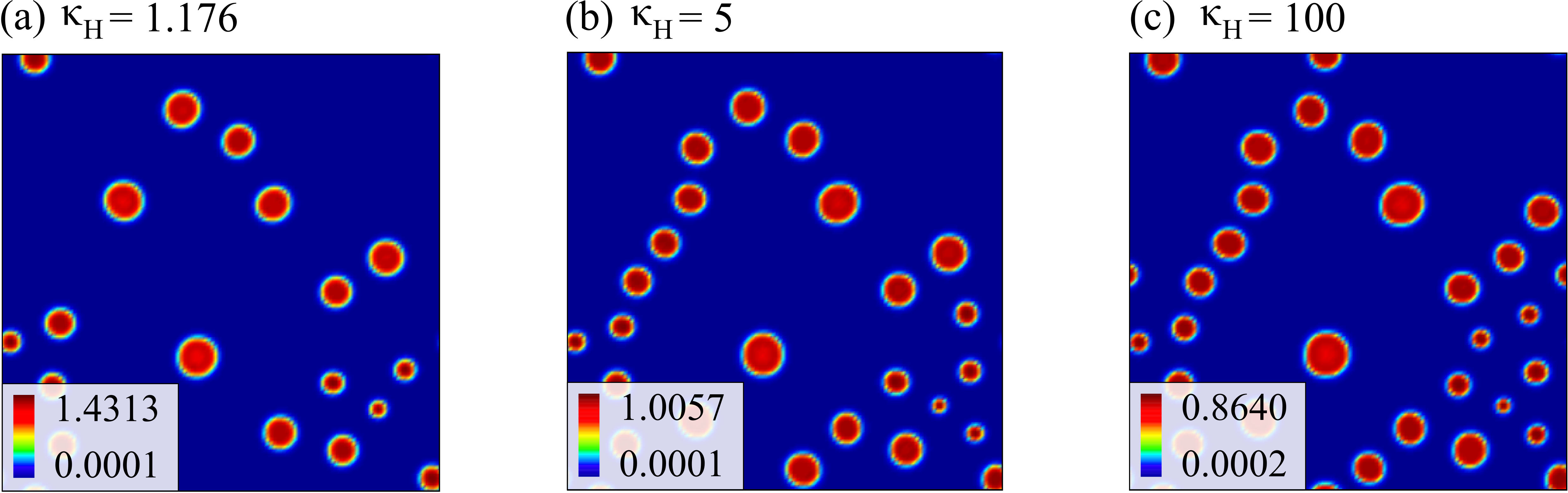
Figure 6: Color coded two-dimensional solvent-phobic density profiles $\phi_{B}$ of stable micelles for different compressive moduli $\kappa_{H}=1.176$ (a), $\kappa_{H}=5$ (b) and $\kappa_{H}=100$ (c). Simulations were performed on a $128\times 128$ grid with a lattice constant $\Delta l=\nicefrac{{1}}{{3}}$ and a fixed time step of $h=0.002$. The values of the remaining parameters are $\chi_{BS}=1.6$, $f_{P}=0.1$, $N_{A}=2$, $N_{B}=15$, $\chi_{AB}=1.05$, $\chi_{AS}=0.0375$, $D_{P}=\nicefrac{{1}}{{N}}$, and $D_{S}=1$. All snapshots are taken at time step $n=200000$.

The value of the compressive modulus $\kappa_{H}$ affects the number, the mean size, and the polymer content of simulated nanoparticles as shown in figure 6.

 

$$\left[1-hD_{P}\left((1+2\tilde{\kappa}_{H}\phi_{A}^{(n)})\Delta-4\beta_{A}\tilde{\kappa}_{H}\phi_{A}^{(n)}\nabla\omega_{A}^{(n)}\cdot\nabla\right)\right]\omega_{A}^{(n+1)}-\left[hD_{P}\tilde{\kappa}_{H}2\phi_{B}^{(n)}\left(\Delta-2\beta_{B}\nabla\omega_{B}^{(n)}\cdot\nabla\right)\right]\omega_{B}^{(n+1)}$$

$$-\left[hD_{P}\tilde{\kappa}_{H}\phi_{S}^{(n)}(\Delta-\beta_{S}\nabla\omega_{S}^{(n)}\cdot\nabla)\right]\omega_{S}^{(n+1)}=\omega_{A}^{(n)}-hD_{P}E_{A}^{(n)},$$ (19)

$$-\left[hD_{P}\tilde{\kappa}_{H}2\phi_{A}^{(n)}\left(\Delta-2\beta_{A}\nabla\omega_{A}^{(n)}\cdot\nabla\right)\right]\omega_{A}^{(n+1)}+\left[1-hD_{P}\left((1+2\tilde{\kappa}_{H}\phi_{B}^{(n)})\Delta-4\beta_{B}\tilde{\kappa}_{H}\phi_{B}^{(n)}\nabla\omega_{B}^{(n)}\cdot\nabla\right)\right]\omega_{B}^{(n+1)}$$

$$-\left[hD_{P}\tilde{\kappa}_{H}\phi_{S}^{(n)}\left(\Delta-\beta_{S}\nabla\omega_{S}^{(n)}\cdot\nabla\right)\right]\omega_{S}^{(n+1)}=\omega_{B}^{(n)}-hD_{P}E_{B}^{(n)},$$ (20)

$$-\left[hD_{S}\tilde{\kappa}_{H}2\phi_{A}^{(n)}\left(\Delta-2\beta_{A}\nabla\omega_{A}^{(n)}\cdot\nabla\right)\right]\omega_{A}^{(n+1)}-\left[hD_{S}\tilde{\kappa}_{H}2\phi_{B}^{(n)}\left(\Delta-2\beta_{B}\nabla\omega_{B}^{(n)}\cdot\nabla\right)\right]\omega_{B}^{(n+1)}$$

$$+\left[1-hD_{S}\left((1+\tilde{\kappa}_{H}\phi_{S}^{(n)})\Delta-\beta_{S}\tilde{\kappa}_{H}\phi_{S}^{(n)}\nabla\omega_{S}^{(n)}\cdot\nabla\right)\right]\omega_{S}^{(n+1)}=\omega_{S}^{(n)}-hD_{S}E_{S}^{(n)}.$$ (21)

 

Figure 7: Semi-implicit integrator for the potential field equations 9 to increase stability regions at high $\kappa_{H}$.

Polymer solutions typically possess a liquid-like compressive modulus Freed.1995 , so simulations should be performed at high $\kappa_{H}$. If the chemical potentials $\mu_{i}$ from equations 10 – 12 are inserted into the dynamical equations 9, $\kappa_{H}$ appears as a prefactor of Laplacian terms $\Delta\phi_{i}$. Hence, the stiffness of the dynamical equations increases with $\kappa_{H}$. Stiffness of differential equations can be tackled by applying implicit or semi-implicit numerical integration schemes Dahlquist.1963 ; Zhu.1999 ; Ascher.1995 ; Uneyama.2007 .

A standard approach Dahlquist.1963 ; Zhu.1999 ; Ascher.1995 to cope with the stiffness caused by high $\kappa_{H}$ in equation (9) is to carry out a direct implicit quadrature of the term $\int_{t_{n}}^{t_{n+1}}\kappa_{H}\left(\Delta\phi_{A}(t)+\Delta\phi_{B}(t)+\Delta\phi_{S}(t)\right)\,dt$ upon integrating the equation over a time step $h=t_{n+1}-t_{n}$. Hence, the right hand side of the time discrete version of equation (9) depends on $\phi_{i}^{(n+1)}$, which in turn depends on $\omega_{i}^{(n+1)}$ via the (discretized) equations (3) and (6 – 8). Here $\phi_{i}^{(n)}\approx\phi_{i}(t_{n})$ and $\omega_{i}^{(n+1)}\approx\omega_{i}(t_{n+1})$ describe the discrete evolution of $\phi_{i},\omega_{i}$ in the time discrete dynamics. In order to solve equation (9) for $\omega_{i}^{(n+1)}$, one must thus solve the whole complexly nested non-linear system of the discretized equations (3), (6 – 8), and (9) by an interative method. The unknowns of the SCF-EPD model are $\omega_{i}^{(n+1)}(\vec{r})$, $\phi_{i}^{(n+1)}(\vec{r})$, $g^{(n+1)}(\vec{r},s)$, and $g^{\prime(n+1)}(\vec{r},s)$ with $i=A,B,S$ at all $m$ spatial grid points and discretized positions $s=n\,ds$ of distance $ds=\nicefrac{{1}}{{N}}$ along a polymer chain with $n\in\{0,...,N\}$. It is evident that the number of unknowns and thus, the dimension of the discretized system of equations, increases dramatically with the polymer chain length $N$. In fact, the iteration along the polymer chain for every $\vec{r}$ to calculate $g$ and $g^{\prime}$ typically consumes by far the most part of the computation time even for algebraic update rules from explicit integrators for equation (3). Therefore, solving the complete set of equations (3), 6 – 8, and 9 by an iterative method would lead to a particularly dramatic increase of simulation times with growing $N$.

Hence, implicit iterative schemes that involve multiple calculations of $\phi_{i}^{(n+1)}$ help to overcome stiffness instabilities at high values of $\kappa_{H}$, but they come at the cost of a dramatic increase in computation times. To avoid this problem while still enlarging the $\kappa_{H}$-region where the the algorithm runs stably, we have developed a semi-implicit integrator for equation (9) that does not require the computation of $\phi_{i}^{(n+1)}$. The main equations are summarized in figure 7 (equations (19–21)), the derivation will be shown below. In this scheme, the potential fields $\omega_{i}^{(n+1)}(\vec{r})$ are decoupled from the other unkown variables $\phi_{i}^{(n+1)}(\vec{r})$, $g^{(n+1)}(\vec{r},s)$, and $g^{\prime(n+1)}(\vec{r},s)$. This decoupling allows one to selectively deal with $\kappa_{H}$-induced stiffness of the dynamical equations while keeping the computational effort per time step as close to efficient explicit schemes as possible. In other words, it guarantees that, in particular, $g^{(n+1)}(\vec{r},s)$ and $g^{\prime(n+1)}(\vec{r},s)$ can still be calculated by cost-efficient explicit schemes, whereas the iterative methods are only applied to a $3m$-dimensional system of equations for $\omega_{i}(\vec{r},t_{n+1})$. At $\kappa_{H}=100$, our semi-implicit integration scheme allows us to use much larger time steps than, e.g., the explicit scheme used in earlier work He.2006 , and as a result, the simulations are up to 100 times faster simon_diss . We solve equation (3) with the explicit scheme from Tzemeres et al. Tzeremes.2002 and to calculate $\phi_{i}$, the integrals in equations (6 – 8) are approximated by a standard Euler method.

The first step in the derivation of this integrator from equation (9) is to extract explicit $\omega_{i}$-expressions from $\Delta\phi_{i}$. Equation (8) directly yields the exact relation

$$\Delta\phi_{S}=\phi_{S}\left[\nabla\omega_{S}\cdot\nabla\omega_{S}-\Delta\omega_{S}\right].$$ (22)

To obtain analogous expressions for $\Delta\phi_{A}$ and $\Delta\phi_{B}$ we apply the Feynman-Kac formula. It states that solutions to equation (3) can be defined recursively by

$$\begin{split}g[\omega](\vec{r},s)=&\exp\left(-dsN\omega(\vec{r})\right)\int_{V}\Phi(\vec{r}-\vec{r}\,^{\prime})g[\omega](\vec{r}\,^{\prime},s-ds)d\vec{r}\,^{\prime}\\ \eqqcolon&\exp\left(-dsN\omega(\vec{r})\right)\,I[\omega](\vec{r}),\end{split}$$ (23)

where $\Phi$ is proportional to the bond transition probability of a Gaussian chain Fredrickson.2006 and $\omega$ is given by equation (4). Likewise, one has

$$g^{\prime}[\omega](\vec{r})=\exp(-dsN\omega)\,I^{\prime}[\omega](\vec{r})$$ (24)

with $\omega$ from equation (5). Inserting the recursive definitions of the end segment distribution functions from equations (23) and (24) into the respective equation (6) or (7) yields

$$\Delta\phi_{i}=\phi_{i}\left[4dsN\nabla\omega_{i}\cdot\nabla\omega_{i}-2dsN\Delta\omega_{i}\right]+R_{i}$$ (25)

for $i=A\text{, }B$. The remainder $R_{i}$ summarizes all non-leading stiffness contributions, which in this case are all terms that contain derivatives of the integrals $I$ and $I^{\prime}$ with respect to the entries $r_{j}$ of $\vec{r}=(r_{1},r_{2},r_{3})^{T}$. Since we use $ds=\nicefrac{{1}}{{N}}$ in our simulations, we set $dsN=1$. In the following we use the short hand notations

$$X_{S}=\Delta\omega_{S}-\beta_{S}\nabla\omega_{S}\cdot\nabla\omega_{S}$$ (26)

and

$$X_{i}=2\Delta\omega_{i}-\beta_{i}4\nabla\omega_{i}\cdot\nabla\omega_{i}$$ (27)

for $i=A\text{, }B$, where $\beta_{A}$, $\beta_{B}$, $\beta_{S}\in[0,1]$ are damping coefficients to adjust the ’degree’ of the implicit treatment and to regulate truncation errors: the smaller the damping coefficients, the smaller are truncation errors. To prepare the dynamical equations (9) for the semi-implicit integrator we define $\tilde{\kappa}_{H}=\alpha\kappa_{H}$ with another damping coefficient $\alpha\in[0,1]$ and zero-pad their time integrals according to

$$\begin{split}\omega_{i}(t_{n+1})&=\,\omega_{i}(t_{n})-D_{i}\int_{t_{n}}^{t_{n+1}}\Big{\{}\Delta\mu_{i}\\ &+\Delta\omega_{i}+\tilde{\kappa}_{H}\left(\phi_{A}X_{A}+\phi_{B}X_{B}+\phi_{S}X_{S}\right)\Big{\}}\,dt\\ &+D_{i}\int_{t_{n}}^{t_{n+1}}\Big{\{}\Delta\omega_{i}+\tilde{\kappa}_{H}\left(\phi_{A}X_{A}+\phi_{B}X_{B}+\phi_{S}X_{S}\right)\Big{\}}\,dt\end{split}$$ (28)

Since the first integral on the right hand side of equation (28) contains the chemical potential minus the leading stiffness contributions, we approximate it by an explicit Euler formula, i.e.

$$\begin{split}&\int_{t_{n}}^{t_{n+1}}\Big{\{}\Delta\mu_{i}+\Delta\omega_{i}+\tilde{\kappa}_{H}\left(\phi_{A}X_{A}+\phi_{B}X_{B}+\phi_{S}X_{S}\right)\Big{\}}\,dt=\\ &h\Big{\{}\Delta\mu_{i}^{(n)}+\Delta\omega_{i}^{(n)}+\tilde{\kappa}_{H}\left(\phi_{A}^{(n)}X_{A}^{(n)}+\phi_{B}^{(n)}X_{B}^{(n)}+\phi_{S}^{(n)}X_{S}^{(n)}\right)\Big{\}}\\ &\eqqcolon hE_{i}^{(n)}.\end{split}$$ (29)

The second integral on the right hand side of equation (28) is treated semi-implicitly. To approximate the included integrals $\int\phi_{i}X_{i}\,dt$ we use the quadrature formulas

$$\int_{t_{n}}^{t_{n+1}}\phi_{i}\Delta\omega_{i}\,dt\approx\phi^{(n)}\Delta\omega_{i}^{(n+1)}h$$ (30)

and

$$\int_{t_{n}}^{t_{n+1}}\phi_{i}\nabla\omega_{i}\cdot\nabla\omega_{i}\,dt\approx\phi_{i}^{(n)}\nabla\omega_{i}^{(n)}\cdot\nabla\omega_{i}^{(n+1)}h,$$ (31)

which are first order time accurate. The first $\nabla\omega_{i}$ on the right hand side of equation (31) is treated explicitly to obtain a linear system of equations for $\omega_{i}^{(n+1)}$. Inserting the short hand notations from equations (26), (27), and (29) together with the quadrature formulas (30) and (31) into equation (28) yields the semi-implicit integration scheme shown in figure 7, equations (19), (20), and (21)).

Spatial derivatives are discretized by a second order finite differences. To solve the resulting discrete linear system of equations for $\omega_{i}^{(n+1)}(\vec{r})$ we use the Generalized Minimal Residual Method (GMRES), which is a Krylow subspace iteration method for linear systems with positive semidefinite matrices and known to be efficient and robust Saad.1986 . In our particular implementation a Krylow iteration is considered to have converged once the residual drops below $10^{-10}$ or the maximum number of 50 iterative steps is reached. In case the residual is still above $10^{-8}$ after 50 steps, we decrease the width of subsequent time steps by multiplication with $1/1.5$. Further details on the implementation of the algorithm can be found in simon_diss . We set the damping coefficients to $\alpha=0.5$ and $\beta_{A}=\beta_{B}=\beta_{S}=0$. For this choice, the simulations in the present work are found to be sufficiently stable.

REFERENCES

REFERENCES

- (1) D. M. Herlach, I. Klassen, P. Wette, and D. Holland-Moritz. Colloids as model systems for metals and alloys: A case study of crystallization. Journal of Physics: Condensed Matter, 22(15):153101, 2010.
- (2) F. Smallenburg, N. Boon, M. Kater, M. Dijkstra, and R. Roij. Phase Diagrams of Colloidal Spheres with a Constant Zeta-Potential. Journal of Chemical Physics, 134:074505, 2011.
- (3) M. A. Bucaro, P. R. Kolodner, J. A. Taylor, A. Sidorenko, J. Aizenberg, and T. N. Krupenkin. Tunable Liquid Optics: Electrowetting-Controlled Liquid Mirrors Based on Self-Assembled Janus Tiles. Langmuir, 25(6):3876–3879, 2009.
- (4) D. Lensen, D. M. Vriezema, and van Hest, J. C. M. Polymeric Microcapsules for Synthetic Applications. Macromolecular Bioscience, 8(11):991–1005, 2008.
- (5) D. E. Discher and A. Eisenberg. Polymer Vesicles. Science, 297:967–972, 2002.
- (6) L. Zhang, F. X. Gu, J. Chan, A. Z. Wang, R. S. Langer, and O. Farokhzad. Nanoparticles in Medicine: Therapeutic Applications and Developments. Clinical Pharmacology and Therapeutics, 83:761–769, 2008.
- (7) M. E. Gindy and R. K. Prud’homme. Multifunctional nanoparticles for imaging, delivery and targeting in cancer therapy. Expert Opinion on Drug Delivery, 6(8):865–878, 2009.
- (8) P. Vartholomeos, M. Fruchard, A. Ferreira, and C. Mavroidis. MRI-Guided Nanorobotic Systems for Therapeutic and Diagnostic Applications. Annual Review of Biomedical Engineering, 13(1):157–184, 2011.
- (9) T. M. Allen and P. R. Cullis. Drug Delivery Systems: Entering the Mainstream. Science, 303:1818–1822, 2004.
- (10) R. Bleul. Herstellung, Characterisierung und Funktionalisierung polymerer Nanopartikel und Untersuchung der Wechselwirkung mit biologischen Systemen. Dissertation, Freie Universität Berlin, 2014.
- (11) B. M. Discher, Y. Y. Won, D. S. Ege, J. C. M. Lee, F. S. Bates, D. E. Discher, and D. A. Hammer. Polymersomes: Tough Vesicles Made from Diblock Copolymers. Science, 284:1143–1146, 1999.
- (12) R. Thiermann. Selbstorganisation amphiphiler Block-Copolymere in Mikromischern. Dissertation, Berlin University of Technology, 2014.
- (13) R. Thiermann, W. Müller, A. Montesinos-Castellanos, D. Metzke, P. Löb, V. Hessel, and M. Maskos. Size controlled polymersomes by continuous self-assembly in micromixers. Polymer, 53(11):2205–2210, 2012.
- (14) S. Tenzer, D. Docter, S. Rosfa, A. Wlodarski, J. Kuharev, A. Rekik, S. K. Knauer, C. Bantz, T. Nawroth, C. Bier, J. Sirirattanapan, W. Mann, L. Treuel, R. Zellner, M. Maskos, H. Schild, and R. H. Stauber. Nanoparticle Size Is a Critical Physicochemical Determinant of the Human Blood Plasma Corona: A Comprehensive Quantitative Proteomic Analysis. ACS Nano, 5(9):7155–7167, 2011.
- (15) H. Maeda, J. Wu, T. Sawa, Y. Matsumura, and K. Hori. Tumor vascular permeability and the epr effect in macromolecular therapeutics: a review. Journal of Controlled Release, 65:271–284, 2000.
- (16) C. Zhang, V. J. Pansare, R .K. Prud’homme, and R. D. Priestley. Flash nanoprecipitation of polysterene nanoparticles. Soft Matter, 8:86–93, 2012.
- (17) W. Müller. Hydrophobe und hydrophile Beladung polymerer Vesikel. Dissertation, Johannes Gutenberg University Mainz, 2009.
- (18) A. Nikoubashman, V. E. Lee, C. Sosa, R. K. Prud’homme, R. D. Priestley, and A. Z. Panagiotopoulos. Directed Assembly of Soft Colloids through Rapid Solvent Exchange. ACS Nano, 10:1425–1433, 2016.
- (19) L. Falk and J. M. Commenge. Performance comparison of micromixers. Chemical Engineering Science, 65(1):405–411, 2010.
- (20) K. S. Drese. Optimization of interdigital micromixers via analytical modeling—exemplified with the SuperFocus mixer. Chemical Engineering Journal, 101(1-3):403–407, 2004.
- (21) F. Schönfeld, K. S. Drese, S. Hardt, V. Hessel, and C. Hofman. Optimized distributive -mixing by ’chaotic’ multilamination. NSTI-Nanotech, 1:378–381, 2004.
- (22) S. Keßler. Dissertation Universität Mainz, 2017. in preparation.
- (23) S. Keßler, F. Schmid, and K. Drese. Modeling size controlled nanoparticle precipitation with the co-solvency method by spinodal decomposition. Soft Matter, 12:7231 – 7240, 2016.
- (24) M. E. Wall, M. C. Wani, C. E. Cook, K. H. Palmer, McPhail A. T., and G. A. Sim. Plant Antitumor Agents. I. The Isolation and Structure of Camptothecin, a Novel Alkaloidal Leukemia and Tumor Inhibitor from Camptotheca acuminata. Journal of American Chemical Society, 88:3888 – 3890, 1966.
- (25) V. P. Torchilin. Recent advances with liposomes as pharmaceutical carriers. Nature Review Drug Discovery, 4:145 – 160, 2005.
- (26) W. Müller, K. Koynov, S. Pierrat, R. Thiermann, C. Fischer, and M. Maskos. pH-change protective PB-b-PEO polymersomes. Polymer, 52:1263 – 1267, 2011.
- (27) A. V. Kabanov, E. V. Batrakova, and V. Y. Alakhov. Pluronic((R)) block copolymers for overcoming drug resistance in cancer. Advanced Drug Delivery Reviews, 54:759 – 779, 2002.
- (28) N. M. Maurits and J. G. E. M. Fraaije. Mesoscopic dynamics of copolymer melts: From density dynamics to external potential dynamics using nonlocal kinetic coupling. The Journal of Chemical Physics, 107(15):5879, 1997.
- (29) X. He and F. Schmid. Dynamics of Spontaneous Vesicle Formation in Dilute Solutions of Amphiphilic Diblock Copolymers. Macromolecules, 39(7):2654–2662, 2006.
- (30) X. He and F. Schmid. Spontaneous Formation of Complex Micelles from a Homogeneous Solution. Physical Review Letters, 100(13), 2008.
- (31) M. Müller and F. Schmid. Incorporating Fluctuations and Dynamics in Self-Consistent Field Theories for Polymer Blends. In Advances in Polymer Science, volume 185, pages 1–85. Springer Verlag, 2005.
- (32) S. F. Edwards. The statistical mechanics of polymers with excluded volume. Proceedings of the Physical Society, 85:613 – 624, 1965.
- (33) F. Schmid. Self-consistent-field theories for complex fluids. Journal of Physics: Condensed Matter, 10:8105–8138, 1998.
- (34) E. Helfand. Theory of inhomogeneous polymers: Fundamentals of the Gaussian random-walk model. The Journal of Chemical Physics, 62(3):999, 1975.
- (35) E. Helfand and Y. Tagami. Theory of the Interface between Immiscible Polymers. II. The Journal of Chemical Physics, 56(7):3592, 1972.
- (36) G. H. Fredrickson. The Equilibrium Theory of Inhomogeneous Polymers. Oxford University Press, 2006.
- (37) K. Kawasaki and K. Sekimoto. Dynamical Theory of Polymer Melt Morphology. Physica, 143A:349–413, 1987.
- (38) T. Uneyama. Density functional simulation of spontaneous formation of vesicle in block copolymer solutions. The Journal of Chemical Physics, 126(11):114920, 2007.
- (39) T. M. Weiss, T. Narayanan, and M. Gradzielski. Dynamics of spontaneous vesicle formation in fluorocarbon and hydrocarbon surfactant mixtures. Langmuir, 24(8):3759–3766, APR 15 2008.
- (40) D. J. Adams, S. Adams, D. Atkins, M. F. Butler, and S. Furzeland. Impact of mechanism of formation on encapsulation in block copolymer vesicles. J. Contr. Release, 128(2):165–170, 2008.
- (41) J. Gummel, M. Sztucki, T. Narayanan, and M. Gradzielski. Concentration dependent pathways in spontaneous self-assembly of unilamellar vesicles. Soft matter, 7(12):5731–5738, 2011.
- (42) V. Sofonea and K. R. Mecke. Morphological characterization of spinodal decomposition kinetics. The European Physical Journal B, 8(1):99–112, 1999.
- (43) T. T. Nielsen. An Implementation Of The Connected Component Labelling Algorithm. https://www.codeproject.com/articles/825200/an-implementation-of-the-connected-component-label, 2014.
- (44) H. Mantz, K. Jacobs, and K. Mecke. Utilizing Minkowski functionals for image analysis: A marching square algorithm. Journal of Statistical Mechanics: Theory and Experiment, 2008(12):P12015, 2008.
- (45) J. Heuser, G. J. A. Sevink, and F. Schmid. Self-assembly of polymeric particles in poiseuille flow: A hybrid lattice boltzmann/external potential dynamics simulation study. Macromolecules, 50(11):4474–4490, 2017.
- (46) J. J. van Franeker, G. H. L. Heintges, C. Schaefer, G. Portale, W. Li, M. M. Wienk, P. van der Schoot, and R. A. J. Janssen. Polymer Solar Cells: Solubility Controls Fiber Network Formation. Journal of the American Chemical Society, 137:11783–11794, 2015.
- (47) K. F. Freed. Interrelation between density functional and self-consistent-field formulations for inhomogeneous polymer systems. The Journal of Chemical Physics, 103(8):3230, 1995.
- (48) G. Dahlquist. A special stability problem for linear multistep methods. Communications of the ACM, 14(3):176–179, 1963.
- (49) J. Zhu, L. Q. Shen, J. Shen, and V. Tikare. Coarsening kinetics from a variable-mobility Cahn-Hilliard equation: Application o fa semi-implicit Fourier spectral method. Physical Review E, 60(4):3564–3572, 1999.
- (50) U. M. Ascher, S. J. Ruuth, and B. T. R. Wetton. Implicit-explicit methods for time-dependent partial differential equations. SIAM Journal on Numerical Analysis, 32(3):797–823, 1995.
- (51) G. Tzeremes, K. O. Rasmussen, T. Lookman, and A. Saxena. Efficient computation of the structural phase behavior of block copolymers. Physical Review E, 65:041806 1–5, 2002.
- (52) Y. Saad and M. H. Schlutz. GMRES: A generalized minimal residual algorithm for solving nonsymmetric linear systems. SIAM Journal on Scientific and Statistical Computing, 7:856–869, 1986.