Variational 3D-PIV with Sparse Descriptors

Abstract

3D Particle Imaging Velocimetry (3D-PIV) aim to recover the flow field in a volume of fluid, which has been seeded with tracer particles and observed from multiple camera viewpoints.

The first step of 3D-PIV is to reconstruct the 3D locations of the tracer particles from synchronous views of the volume. We propose a new method for iterative particle reconstruction (IPR), in which the locations and intensities of all particles are inferred in one joint energy minimization. The energy function is designed to penalize deviations between the reconstructed 3D particles and the image evidence, while at the same time aiming for a sparse set of particles. We find that the new method, without any post-processing, achieves significantly cleaner particle volumes than a conventional, tomographic MART reconstruction, and can handle a wide range of particle densities.

The second step of 3D-PIV is to then recover the dense motion field from two consecutive particle reconstructions. We propose a variational model, which makes it possible to directly include physical properties, such as incompressibility and viscosity, in the estimation of the motion field. To further exploit the sparse nature of the input data, we propose a novel, compact descriptor of the local particle layout. Hence, we avoid the memory-intensive storage of high-resolution intensity volumes. Our framework is generic and allows for a variety of different data costs (correlation measures) and regularizers. We quantitatively evaluate it with both the sum of squared differences (SSD) and the normalized cross-correlation (NCC), respectively with both a hard and a soft version of the incompressibility constraint.

1 Introduction

Experimental fluid dynamics requires a measurement system to observe the flow in a fluid. The main method to reconstruct the dense flow field in a (transparent) volume of fluid is to inject neutral-buoyancy tracer particles, tune the illumination to obtain high contrast at particle silhouettes, and record their motion with multiple high-speed cameras. The flow is then reconstructed either by Particle Tracking Velocimetry (PTV) [1], meaning that one follows the trajectories of individual particles and interpolates the motion in the rest of the volume; or by Particle Imaging Velocimetry (PIV) [2, 3], where one directly estimates the local motion everywhere in the volume from the displacements of nearby particle constellations.

Early approaches operated essentially in 2D, focusing on a thin slice of the volume that is selectively illuminated with a laser light-sheet. More recently, it has become common practice to process entire volumes and recover actual 3D fluid motion. A popular variant is to directly lift the problem to 3D by discretizing the volumetric domain into voxels. The standard approach is to process the multi-view video in two steps. First, a 3D particle distribution is reconstructed independently for each frame, often by means of tomographic PIV (Tomo-PIV) [4, 5, 6, 7], and stored as an intensity/probability volume, representing the particle-in-voxel likelihood. A second step then recovers motion vectors, by densely matching the reconstructed 3D particles (respectively, particle likelihoods) between consecutive time frames. The most widely used approach for the latter step is local matching of relatively large interrogation volumes, followed by various post-processing steps, e.g. [4, 8, 9]. In computer vision terminology, this corresponds to the classic Lucas-Kanade (LK) scheme for optical flow computation [10]. While LK is no longer state-of-the-art for 2D flow, it is still attractive in the 3D setting, due to its simplicity, and to the efficiency inherent in a purely local model that lends itself to parallel computation. Optical flow, i.e., dense reconstruction of apparent motion in the 2D image plane, is one of the most deeply studied problems in computer vision. Countless variants have been developed and have found their way into practical applications, such as medical image registration, human motion analysis and driver assistance. The seminal work of Horn and Schunk [11], and its contemporary descendants, e.g. [12, 13, 14], address the problem from a variational perspective. A setting we also follow here. Flow estimation from images is locally underconstrained (aperture problem). Imperfect particle reconstructions and the ambiguity between different, visually indistinguishable, particles further complicate the task. The normal solution for such an ill-posed, inverse problem is to introduce prior knowledge that further constrains the result and acts as a regularizer.

Indeed, modeling the problem in the volumetric domain opens up the possibility to incorporate physical constraints into the model, e.g., one can impose incompressibility of the fluid. These advantages were first pointed out in [15]. [16] were among the first to exploit physical properties of fluids, however, only as a post-process to refine an initial solution obtained with taking into account the physics. Following our own previous work [17], we base regularization on the specific properties of liquids and propose an energy, whose optimality conditions correspond to the stationary Stokes equations of fluid dynamics. This strictly enforces a divergence-free flow field and additionally penalizes the squared gradient of the flow, making explicit the viscosity of the fluid.

Figure 1 depicts our basic setup, a 2-pulse variational flow estimation approach from initial 3d reconstructions.

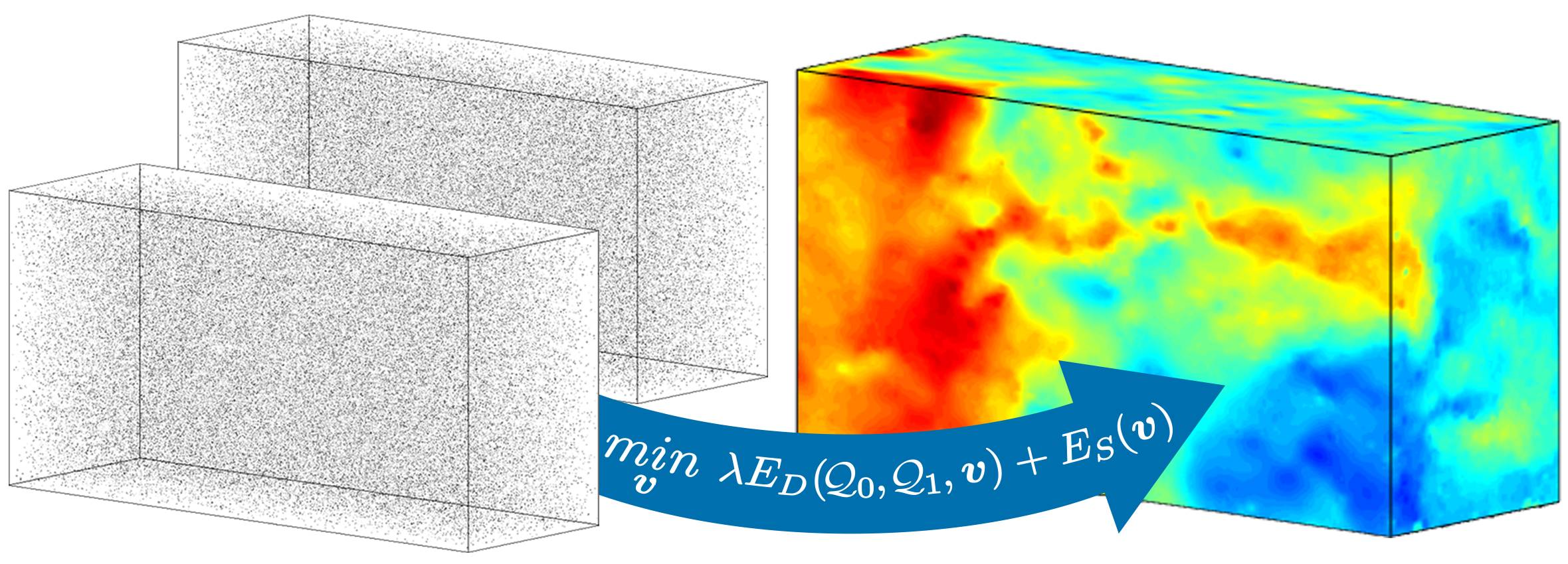
Figure 1: Variational flow estimation from 3d particle reconstructions of two time steps.

By operating densely in the 3D domain, our approach stands in stark contrast with methods that build sparse particle trajectories over multiple time-steps from image domain data [18]. Here, 3D information is used only for matching, in particular to constrain the local search for matching particles in the temporal domain, while regularization is introduced by demanding for smooth 2D trajectories. Physical properties like incompressibility are much harder to model without the consideration of 3D spatial proximity. Hence, these methods have to fit a dense, volumetric representation to the discovered, sparse particle tracks in a separate step. There, relevant physical constraints [19, 20] can be included, yet cannot influence the particles’ 3D motion any more. While multi-frame analysis is certainly well-suited to improve the accuracy and robustness of PIV over long observation times, we argue that the basic case of two (or generally, few) frames is better captured by dense flow estimation in 3D.

The proposed variational energy naturally fits well with modern proximal optimization algorithms [17], and it produces only little memory overhead, compared to conventional window-based tracking in 3D [4, 8] without a-priori constraints. In particular, we have shown in [17] that the sparsity of the particle data and the relative smoothness of the 3D motion field requires highest resolution only for matching. The 3D motion field can therefore be parameterized at a lower resolution, such that the whole optimization part requires about one order of magnitude less memory than storing the intensity volume.

According to the classical variational formulation [11], matching should directly consider the smallest entities (pixel in 2D, voxel in 3D) in the scene. However, particles are sparsely distributed and of high ambiguity, such that one rather compares a constellation of particles in a larger interrogation volume, trading off robustness for matching accuracy. Note that, compared to purely local methods [4, 8], our global model also allows us to consider a smaller neighborhood size for matching.

A popular alternative to matching raw spatial windows is to compress the local intensity patterns into descriptors, e.g. [21, 22]. A descriptor can be designed to support robust matching of different entities, like key-points in different views [23], pedestrians [22] or to provide robustness against illumination changes [24]. Descriptors also improve optical flow computation in several real-world settings [25]. Here, we construct our own descriptor specifically for 3D-PIV, that seeks to balance precision and robustness.

Our descriptor can be constructed on-the-fly and does not require storage of a high-resolution intensity volume, rather it works directly on the locations and intensities of individual particles. Recall that the resolution of the intensity voxel grid [4, 8, 17], is directly coupled to the maximal precision of the estimated motion – this dependency is overcome by the new descriptor. At typical particle densities, constructing descriptors on-the-fly saves about three orders of magnitude in memory (compared to a conventional voxel volume), but obtains comparable precision of the motion field. Moreover, it allows one to fully exploit our memory-efficient optimization procedure.

Although a particle-based representation can also be extracted from tomographic methods [26], it appears more natural to directly reconstruct the particles from the multi-view image data. Iterative particle reconstruction methods (IPR), e.g. [27], deliver exactly that, and often outperform Tomo-PIV methods especially in particle localization accuracy [27]. Building on these ideas, we pose IPR as an optimization problem. Since such a direct energy formulation is highly non-convex, we add a proposal generation step that instantiates new candidate particles. That step is alternated with energy optimization. The energy is designed to explain intensity peaks that are consistent across all views; while at the same time discarding spurious particles that are not supported by sufficient evidence, with the help of a sparsity prior. Especially at large particle densities, our novel IPR-based technique outperforms a tomographic baseline in terms of recall as well as precision of particles (respectively number of missing and ghost particles), which in turn leads to significantly improved fluid motion.

We also present a deep analysis of our IPR based particle reconstruction model, where we analyze the effect of particle quality and density on the motion estimation, and quantitatively study the influence of the main parameters, including different layouts of the sparse descriptor.

2 Method

We follow Horn and Schunk [11] and cast fluid motion estimation directly as a global energy minimization problem over a (cuboid) 3D domain $\Omega\subset\mathbb{R}^{3}$. Emerging from variational principles, the energy of that inverse problem can be divided into a data fidelity term and a regularizer. As input, the basic model requires a set of 3D particles, reconstructed individually for each time step, see Figure 2. It is described in more detail in Sec. 2.1.

As a baseline for particle reconstruction we utilize a well-known tomographic reconstruction technique (MART) [4], which we briefly describe next at the start of the technical section. Afterwards, we present the novel, energy-based IPR solution, which combines a simple image-based data term with an $\operatorname*{l_{0}}0$ sparsity. At this point we also detail the optimization procedure, which alternates between particle generation and energy minimization. Then follows an explanation of the proposed sparse descriptor, which exploits the low density of the particles within the fluid in Sec. 2.2.

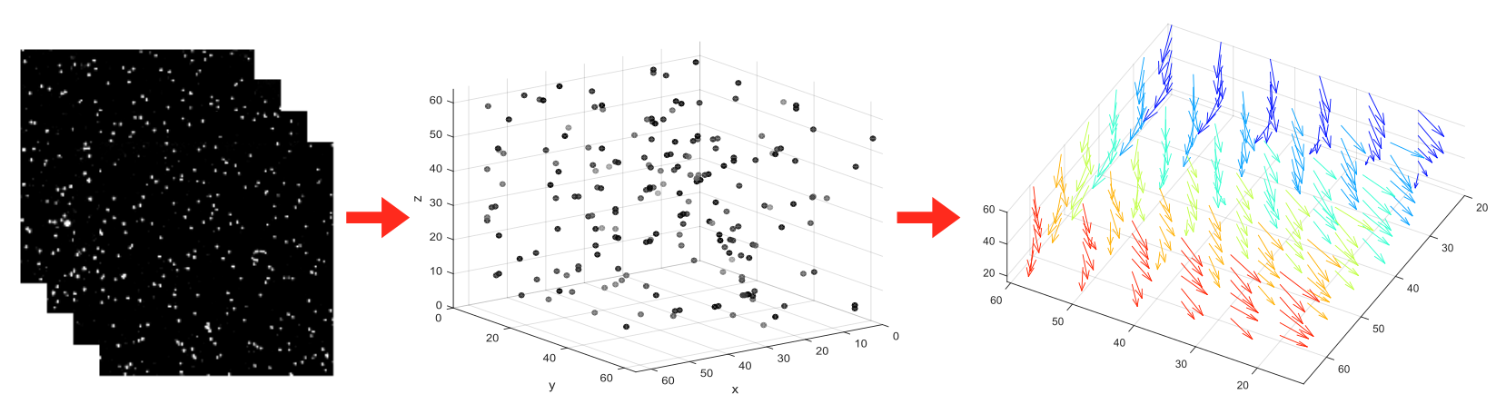
Figure 2: Flow estimation pipeline. (left) 2D input data, (middle) 3D reconstruction, (right) 3D flow estimation from 2 time steps.

The second part, Sec. 2.3, describes the volumetric model for fluid motion estimation. We start with the regularizer which, following [17], is based on the physical properties of the fluid, such as incompressibility and viscosity. Next we review the standard sum-of-squared-distances (SSD) data cost, that we use as a baseline in our framework in Sec. 2.3, and show how our sparse descriptor can instead be integrated into the energy function as data cost. Importantly, the energy is constructed to be convex, in spite of the rather complex data and regularization terms. Hence, it is amenable to a highly efficient optimization algorithm, which we describe at the end of Sec. 2.3.

2.1 3D Reconstruction

The first objective of our pipeline is to reconstruct a set of particles $\mathcal{Q}\!:=\!\{(p_{l},c_{l})\}_{l=1}^{Q}$, consisting of a set of 3D positions $\mathcal{P}\!:=\!\{(p_{l})\}_{l=1}^{Q}$, $p_{l}\!\in\!\mathbb{R}^{3}$ and an associated set of intensities $\mathcal{C}\!:=\!\{(c_{l})\}_{l=1}^{Q}$, $c_{l}\!\in\!\mathbb{R}^{+}$, that together define the data term of the energy function. This is in contrast to voxel-based intensity volumes, e.g. [4]. These dense volumetric representations can be obtained by tomographic reconstruction methods, as traditionally used for 3D-PIV. We compare two techniques to obtain the set of particles: a tomographic method built on MART, and an iterative particle reconstruction (IPR) [27] method that directly obtains sparse 3D particles and intensities from the 2D input images. To extract 3D particle locations and intensities in continuous space from the tomographic MART reconstruction, we perform peak detection and subsequent sub-voxel refinement. Note that the mapping from dense to sparse is invertible, in our experiments we also utilize our IPR variant to generate a high resolution intensity volume on which we define the voxel-based SSD data term [17], as a baseline for our sparse descriptor.

In the following, we assume that the scene is observed by $k=1\ldots K$ calibrated cameras in the images $I_{k}$ and define for each camera a generic projection operator $\Pi_{k}$. To keep the notation simple, we refrain from committing to a specific camera model at this point. However, we point out that fluid dynamics requires sophisticated models to deal with refractions, or alternatively exhaustive calibration to obtain an optical transfer function [28, 29]. Note that we reconstruct the particles individually for each time step, and denote the two consecutive time steps as $t_{0}$ and $t_{1}$.

MART.

Tomographic reconstruction assigns each voxel $i$ of a regular grid $\mathcal{V}$ an intensity value $U(i)$. A popular algebraic reconstruction technique, originally proposed for three-dimensional electron microscopy, is MART [30]. MART solves the convex optimization problem:

$$E_{\textrm{\tiny MART}} (U):=\sum\nolimits_{i\in\mathcal{V}}U(i)\log U(i)\textrm{ subject to }$$ (1)

$$\sum\nolimits_{i\in\mathcal{R}_{j}}\omega_{i,j}U(i)=I_{k}(j)\;\forall k\;\textrm{ and }U(i)\geq 0.$$

Here, $I(j)$ denotes the observed intensity at pixel $j$, $U(i)$ the unknown intensities of voxel $i$, and $\mathcal{R}_{j}$ is the set of all voxels traversed by the viewing ray through pixel $j$. The weight $\omega_{i,j}\!\in\![0,1]$ depends on the distance between the voxel center and the line of sight and is essentially equivalent to an uncertainty cone around the viewing ray, to account for aliasing of discrete voxels. For each pixel $j$ in every camera image $I_{k}$, and for each voxel $i$, the following update step is performed, starting from $U(i)^{0}:=1$:

$$U(i)^{n+1}=U(i)^{n}\cdot\Big{(}I_{k}(j)\Big{/}\sum\nolimits_{i\in\mathcal{R}_{p}}\omega_{i,j}U(i)^{n}\Big{)}^{\omega_{i,j}}.$$ (2)

After each MART iteration, we apply anisotropic Gaussian smoothing ($3\times 3\times 1$ voxels) of the reconstructed volume, to account for elongated particle reconstructions along the $z$-axis due to the camera setup [31]. Furthermore, we found it advantageous to apply non-linear contrast stretching before the subsequent particle extraction or flow computation: $E_{\mathrm{out}}=(E_{\mathrm{in}})^{\gamma}$, with $\gamma=0.7$.

Given the intensity volume $U$, sub-voxel accurate sparse particle locations $\mathcal{P}$ are extracted: first, intensity peaks are found through non-maximum suppression with a $3\times 3\times 3$ kernel, then we fit a quadratic polynomial to the intensity values in a $3\times 3\times 3$ neighborhood.

IPR.

As an alternative to memory-intensive tomographic approaches, IPR methods iteratively grow a set of explicit 3D particles. They are reported to achieve high precision and robustness, cf. [27]. In contrast to the effective, but somewhat heuristic [27], our variant of IPR minimizes a joint energy function over a set of candidate particles to select and refine the optimal particle set. The energy minimization alternates with a candidate generation step, where putative particles are instantiated by analyzing the current residual images (the discrepancies between the observed images and the back-projected 3D particle set). Thus, in every iteration new candidate particles are proposed in locations where the image evidence suggests the presence of yet undiscovered particles. Energy minimization then continually refines particle locations and intensities to match the images, minimizing a data term $E^{D}_{\textrm{\tiny IPR}}(\mathcal{P},\!\mathcal{C})$. At the same time, the minimization also discards spurious ghost particles, through a sparsity prior $E^{S}_{\textrm{\tiny IPR}}$. The overall energy is the sum of both terms, balanced by a parameter $\eta$:

$$E_{\textrm{\tiny IPR}}(\mathcal{P},\mathcal{C}):=E^{D}_{\textrm{\tiny IPR}}(\mathcal{P},\mathcal{C})+\eta E^{S}_{\textrm{\tiny IPR}}(\mathcal{C})$$ (3)

We model particles as Gaussian blobs of variance $\sigma$ and integrate the quadratic difference between prediction and observed image $I_{k}$ over the image plane $\Gamma_{k}$ of camera $k$:

$$E^{D}_{\textrm{\tiny IPR}}(\mathcal{P}\!,\mathcal{C})\!\!:=\!\!\sum_{k=1}^{K}\!\int_{\Gamma_{k}}\!\!\!\!\big{|}\mathcal{I}_{k}(x)\!-\!\!\sum_{l=1}^{Q}\!\Pi_{k}(c_{l}\!\cdot\!\mathcal{N}(p_{l},\sigma)(x)\!)\big{|}_{2}^{2}\mathrm{d}x.$$ (4)

The model in 4 assumes that particles do not possess distinctive material or shape variations. In contrast, we explicitly model the particles’ intensity, which depends on the distance to the light source and changes only slowly. Apart from providing some degree of discrimination between particles, modeling the intensity allows one to impose sparsity constraints on the solution, which reduces the ambiguity in the matching process cf. [32]. In other words, we prefer to explain the image data with as few particles as possible and set

$$E^{S}_{\textrm{\tiny IPR}}(\mathcal{C}):=\sum_{l=1}^{Q}|c_{l}|_{0}+\delta_{\{\geq 0\}}(c_{l}).$$ (5)

The 0-norm in 5 counts the number of particles with non-zero intensity, and has the effect that particles falling below a threshold (modulated by $\eta$) get discarded immediately. In practical settings, the depth range of the observed volume is small compared to the distance to the camera. Consequently, the projection $\Pi$ can be assumed to be (almost) orthographic, such that particles remain Gaussian blobs also in the projection. Omitting constant terms, we can simplify the projection in 4 to

$$\Pi(\mathcal{N}(\cdot,\sigma)(x))\!\approx\!\mathcal{N}(\Pi(\cdot),\sigma)(x)\!\propto\!\frac{1}{\sigma^{2}}\!\exp(\frac{-|\Pi(\cdot)\!-\!x|^{2}}{\sigma^{2}}),$$ (6)

such that we are only required to project the particle center. In practice, we can restrict the area of influence of 6 to a radius of $3\sigma$. While still covering $99.7$% of a particle’s total intensity, this avoids having to integrate particle blobs over the whole image in 3.

Starting from an empty set of particles, our particle generator operates on the current residual images

$$I_{k,\operatorname{res}}\!:=\!\int_{\Gamma_{k}}I_{k}(x)\!-\!\sum_{l=1}^{Q}\!\Pi_{k}(c_{l}\!\cdot\!\mathcal{N}(p_{l},\sigma)(x))\mathrm{d}x$$ (7)

and proceeds as follows: First, peaks are detected in all $k$ 2D camera images. The detection applies non-maximum suppression with a $3\times 3$ kernel and subsequent sub-pixel refinement of peaks that exceed an intensity threshold $\theta$. For one of the cameras, $k\!=\!1$, we shoot rays through each peak and compute their entry and exit points to the domain $\Omega$. In the other views the reprojected entry and exit yield epipolar line segments, which are scanned for nearby peaks. For each constellation of peaks that can be triangulated with a reprojection error $<\epsilon$ in all views, we generate a new (candidate) particle. The initial intensity is set depending on the observed intensity in the reference view, and on the number of candidate particles to which that same peak contributes. In particular, for each of the $m$ detected particles $\{p_{l}\}_{l=1}^{m}$ corresponding to the same peak in the reference, we set $c_{l}\!:=\!\mathcal{I}_{1}(\Pi_{1}(p_{l}))K/(K\!-\!1\!+\!m)$.

We run several iterations during which we alternate proposal generation and energy optimization. Over time, more and more of the evidence is explained, such that the particle generator becomes less ambiguous and fewer candidates per peak are found. We start from a stricter triangulation error $\epsilon$ and increase the value in later iterations.

To minimize the non-convex and non-smooth energy in 3 we apply (inertial) PALM [33, 34]. Being a semi-algebraic function [33, 35], our energy 3 fulfills the Kurdyka-Lojasiewicz property [36], so the sequence generated by PALM is guaranteed to converge to a critical point of 3. To apply PALM we arrange the variables in two blocks, one for the locations of the particles $\mathcal{Q}$ and one for their intensities. This gives two vectors $\mathbf{p}\!:=\!(p_{1}^{\!\mathsf{T}},\ldots,p_{Q}^{\!\mathsf{T}})^{\!\mathsf{T}}\!\in\!\mathbb{R}^{3Q}$ and $\mathbf{c}\!:=\!(c_{1},\ldots,c_{Q})^{\!\mathsf{T}}\!\in\!\mathbb{R}^{Q}$. The energy is already split into a smooth part 4 and non-smooth part 5, where the latter is only a function of one block ($\mathbf{c}$). In this way, we can directly apply the block-coordinate descent scheme of PALM. The algorithm iterates between the two blocks $\mathbf{p}$ and $\mathbf{c}$ and executes the steps of a proximal forward-backward scheme. At first, we take an explicit step w.r.t. one block of variables $z\!\in\!\{\mathbf{p},\mathbf{c}\}$ on the smooth part $E^{D}_{\textrm{\tiny IPR}}$, then take a backward (proximal) step on the non-smooth part $E^{S}_{\textrm{\tiny IPR}}$ w.r.t. the same block of variables – if possible.

That is, at iteration $n$ and $z\in\{\mathbf{p},\mathbf{c}\}$, we perform updates of the form

$$z^{n+1}= \textrm{prox}^{E^{S}_{\textrm{\tiny IPR}}}_{t}(z):=\operatorname*{arg\,min}_{y}E^{S}_{\textrm{\tiny IPR}}(y)+\frac{t}{2}\|y-z\|^{2}$$ (8)

$$\textrm{ with }\quad z=z^{n}-t^{-1}\nabla_{z}E^{D}_{\textrm{\tiny IPR}}(\cdot,z^{n}),$$

with a suitable step size $1/t$ for each block of variables.

Throughout the iterations, we further have to ensure that the step size in the update of a variable block $z\!\in\!\{\mathbf{p},\mathbf{c}\}$ is chosen in accordance with the Lipschitz constant $L_{z}$ of the partial gradient of function $E^{D}_{\textrm{\tiny IPR}}$ at the current solution:

$$\|\nabla_{z}E^{D}_{\textrm{\tiny IPR}}\!(\!\cdot,\!z_{1})\!-\!\nabla_{z}E^{D}_{\textrm{\tiny IPR}}(\!\cdot,\!z_{2})\|\!\leq\!L_{z}(\!\cdot,\!\cdot)\|z_{1}\!-\!z_{2}\|\,\forall z_{1},\!z_{2}.$$ (9)

In other words, we need to verify whether the step size $t$ in 8, used for computing the update $z^{n+1}$, fulfills the descent lemma [37]:

$$E_{\textrm{\tiny IPR}}(\cdot,z^{n+1})\leq E_{\textrm{\tiny IPR}}(\cdot,z^{n})+\langle\nabla_{z}E^{D}_{\textrm{\tiny IPR}}(\cdot,z^{n}),$$ (10)

$$z^{n+1}\!-\!z^{n}\rangle+\frac{t}{2}\|z^{n+1}-z^{n}\|^{2}.$$

Otherwise the update step has to be recalculated with a smaller step size. In practice, the Lipschitz continuity of the gradient 10 of $E^{D}_{\textrm{\tiny IPR}}$ only has to be checked locally at the current solution. Hence, we employ the back-tracking approach of [38], which is provided in pseudo-code in Alg. 1.

Algorithm 1 iPalm implementation for energy (3)

1:procedure ipalm($\mathbf{p}^{0},\mathbf{c}^{0})$

2:     $\mathbf{p}^{-1}\leftarrow\mathbf{p}^{0};\mathbf{c}^{-1}\leftarrow\mathbf{c}^{0};$

3:     $\tau\leftarrow\frac{1}{\sqrt{2}};L_{\mathbf{p}}\leftarrow 1;L_{\mathbf{c}}\leftarrow 1;$

4:     for n:=0 to $n_{\textrm{steps}}$ do

5:         $\mathbf{\hat{p}}\leftarrow\mathbf{p}^{n}+\tau(\mathbf{p}^{n}-\mathbf{p}^{n-1});$ // inertial step

6:         while true do

7:              $\mathbf{p}^{n+1}:=\mathbf{\hat{p}}-1/L_{\mathbf{p}}\nabla_{\mathbf{p}}E^{D}_{\textrm{\tiny IPR}}(\mathbf{\hat{p}},\mathbf{c}^{n});$

8:              if $\mathbf{p}^{n+1},L_{\mathbf{p}}$ fulfill 10 then break;

9:              else $L_{\mathbf{p}}=2L_{\mathbf{p}}$;                        

10:         $\mathbf{\hat{c}}\leftarrow\mathbf{c}^{n}+\tau(\mathbf{c}^{n}-\mathbf{c}^{n-1})$; // inertial step

11:         while true do

12:              $\mathbf{c}:=\mathbf{\hat{c}}-1/L_{\mathbf{c}}\nabla_{\mathbf{c}}E^{D}_{\textrm{\tiny IPR}}(\mathbf{p}^{n+1},\mathbf{\hat{c}});$

13:              $\mathbf{c}^{n+1}:=\textrm{prox}^{F_{\mathbf{c}}}_{L_{\mathbf{c}}}(\mathbf{c})$; // 12

14:              if $\mathbf{c}^{n+1},L_{\mathbf{c}}$ fulfill 10 then break;

15:              else $L_{\mathbf{c}}=2L_{\mathbf{c}}$;                             

For simple proximal operators, like ours, it is recommended to also increase the step sizes as long as they still fulfill 10, instead of only reducing them when necessary (lines 9,15 in Alg. 1). Taking larger steps per iteration speeds up convergence. We also take inertial steps [34] in Alg. 1 (lines 5,10). Inertial methods can provably accelerate the convergence of first-order algorithms for strongly convex energies, improving the worst-case convergence rate from $O(1/n)$ to $O(1/n^{2})$ in $n$ iterations, cf. [38]. Although there are no such guarantees in our non-convex case, these steps significantly reduce the number of iterations in our algorithm by a factor of five, while leaving the computational cost per step practically untouched.

The proximal step on the intensities $\mathbf{c}$ can be solved point-wise. It can be written as the 1D-problem

$$\textrm{prox}^{E^{S}_{\textrm{\tiny IPR}}}_{t}(\bar{c}):=\operatorname*{arg\,min}_{c}\eta|c|_{0}+\delta_{\{\geq 0\}}(c)+\frac{t}{2}|c-\bar{c}|^{2},$$ (11)

which admits for a closed-form solution:

$$\textrm{prox}^{E^{S}_{\textrm{\tiny IPR}}}_{t}(\bar{c}):=\left\{\!\!\begin{array}[]{c@{\hspace{0.2cm}}l}0\hfil\hskip 5.69046pt&\textrm{if }t\bar{c}^{2}\!\!<\!2\eta\textrm{ or }\bar{c}\!<\!0\\ \bar{c}\hfil\hskip 5.69046pt&\textrm{else},\end{array}\right..$$ (12)

2.2 Sparse Descriptor

In PIV, particle constellations are matched between two time steps. To that end, an interrogation window at the location for which one wants to determine velocity is considered as the local “descriptor”. Velocity information is obtained from the spatial displacement between corresponding patches, typically found via (normalized) cross correlation ((N)CC). For 3D-PIV this requires the storage of full intensity voxel volumes, like those obtained with tomographic reconstruction. Discretizing the particle information at this early stage has the disadvantage that the resolution of the voxel grid directly limits the maximal precision of the motion estimate. Especially when considering multiple time steps, storing intensity voxel volumes at high resolution is demanding on memory, although the actual particle data is sparse. Moreover, large window sizes are needed to obtain robust correspondence, which (over-)smoothes the output, trading off precision for robustness. Notably, in practical 3D-PIV these required interrogation volumes are very large, e.g. Elsinga et al. [4] recommend $41^{3}$. For typical particle densities, such an interrogation window contains only 25 particles on average. Finally, IPR-type methods reportedly outperform MART in terms of reconstruction quality, and directly deliver sparse particle output.

These findings motivate us to investigate a new feature descriptor that directly works on the sparse particle data. In order to replace the conventional correlation window, our novel descriptor must be defined at arbitrary positions in $\Omega$ and lead to sub-voxel accurate measurements. To use the descriptor in our variational setup we further demand that it be differentiable. Finally, the descriptor should be independent of the distance metric, such that we can use standard measures like SSD or (negative) NCC.

Similar to an interrogation window, the descriptor considers all particles within a specified distance around its center location. Its structure is defined by a radius $r$, the arrangement of a set of vertices $H$, and an integer count $k$. All particles within a distance smaller than $r$ contribute to the descriptor vector. For such a particle $q=(p,c)$, we further define the set of $k$ nearest neighbors in $H$, $\mathcal{N}^{k}_{H}(p)$, to which the intensity $c$ of the particle is distributed. We weight the contribution of $q$ to the vertex $h\in\mathcal{N}^{k}_{H}(p)$ with a radial distance function $exp(-\|p-h\|/2)$ and normalize the $k$ weights induced by the particle to sum to one. In computer graphics, such a 3D-to-2D projection by weighted soft-assignment is called splatting. Apart from higher precision of the descriptor, cf. [21, 22], the splatting strategy leads to smoother descriptor changes when the nearest neighbor set changes after a spatial displacement of the particle. More importantly, it guarantees that the descriptor is at least piecewise differentiable.

Note, when arranging $H$ in a regular orthogonal grid and setting $k\!=\!8$, the descriptor closely resembles a conventional interrogation volume. Instead, we propose to arrange the vertices on spherical shells with different radii. A 2-dimensional illustration with $k=3$ is shown in Figure 3. Vertices are depicted in red and particles in blue.

Any descriptor is constructed to fulfill some set of desirable properties [39, 40, 41]. Designing one specifically for our application has the advantage that it can be tuned to the specific scenario. In our case we do not seek rotational invariance, and all directions should be considered equally (i.e. same vertex density on poles and equator). Further, our input is unstructured (in contrast to, for instance, laser scan points that adhere to 2D surfaces). Similar to [41] we prefer to distribute the vertices $H$ uniformly on the surface of multiple spheres. Accordingly, we place them at the corners of an icosahedron (or subdivisions of it) for each sphere. We further seek equidistant spacing between neighboring spheres and chose the distance of the radii in accordance with the distances of vertices on the inner shell. Because particles close to the center are more reliable for its precise localization, we place more points towards the descriptor center, for a more fine-grained binning of close particles. In contrast, particles that are further away are more likely have different velocity and are splatted over a wider area. Hence, these particles mainly contribute to disambiguate the descriptor. The precision argument also suggests to weight particle closer to the center more strongly than those further away. Similarly, we compensate the fact that the vertices near the center represent a smaller volume than those further away, by weighting their contributions accordingly. To evaluate our descriptor centered at a given location in $\Omega$, we must detect the particles within a radius $r$ of that location, and also find the $k$ nearest neighbours for each particle within $r$. Recall that in our scheme we pre-compute a set of particles $\mathcal{Q}$ consisting of location and intensity at both time steps. To find the particles we construct a KD-tree [42] once for each time step, to accelerate the search. In our low-dimensional search domain ($\Omega\subset\mathbb{R}^{3}$), with limited number of particles ($\approx 3$ orders of magnitude smaller than voxels in an equivalently accurate intensity volume), the complexity of the search is quite low, $O(\log|\mathcal{Q}|)$. To find the $k$ nearest vertices for each contributing particle we can use a mixed strategy: We partition the descriptor volume into a voxel grid and pre-compute the nearest neighbors for the corners of the voxels, storing the $k$ nearest neighbor if that set is unique. In this way, the $k$-NN search can be done in constant time for a large majority of all cases. To handle the rare case of particles falling in voxels without a unique neighbor set, we pre-compute a KD-tree for the rather small set of vertices $H$ and query the neighbors of the concerned particles. We use the KD-tree implementation proposed in [43]. Overall, we find that, in spite of the need to frequently query nearest neighbours, our descriptor can be evaluated efficiently for any realistic particle density, while saving a lot of memory.

We have tested different layouts and have decided for a structure of six layers. The descriptor vertices are depicted in Figure 3 on the right. On each layer, points are positioned on an icosahedron or subdivisions of it. The point and layer arrangement is described in Table 1. In total the descriptor is a vector $D_{\mathcal{Q}}(x)\in\mathbb{R}^{331}$ with 331 dimensions (vertices).

We empirically chose a radius of $r=10.5$. Note that this leads to a larger influence area than the interrogation volume of $13^{3}$ suggested in [17]. However, in [17] a squared area is used for matching whereas our descriptor has a spherical form. Furthermore, as stated above, particles closer to the descriptor center are weighted higher than further away particles.

Finally we splat the intensity value of each particle over $k=5$ neighbors in the descriptor. Vertices are weighted according to their distance to the descriptor center by $w_{g}=exp(-\|g\|/10)$ and subsequent normalization such that $\sum w_{g}\!=\!1$. We point out that an interrogation volume of comparable metric size, i.e. $17^{3}$ voxels, would consist of 4913 voxels to represent the same particle distribution captured in our 331-dimensional descriptor.

Table 1: Layered structure of our descriptor.

			Distance to	Distance to
Layer	#Points	Radius	neighbor points	lower layer
0	1	0	-	-
1	12	1	1.052	1
2	42	2.205	1.205	1.205
3	92	3.484	1.278	1.278
4	92	5.503	2.019	2.019
5	92	8.693	3.190	3.190

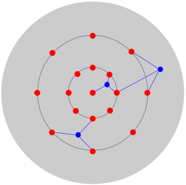
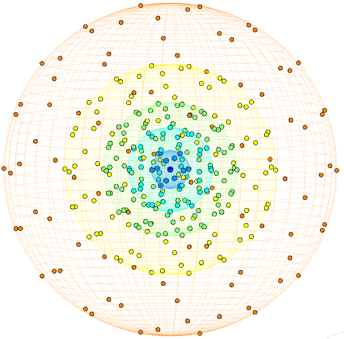
Figure 3: Left: Schematic visualization of a 2D sparse descriptor with descriptor vertices (red) and particle locations (blue), whose intensities are splatted over the 3 nearest neighbors. Right: 3D descriptor vertices (with layer based color-code).

2.3 Volumetric Flow

Motion estimation starts from two particle sets $\mathcal{Q}_{0},\mathcal{Q}_{1}$ for consecutive time steps $t^{0}$ and $t^{1}$, with particles located in the cuboid domain $\Omega\subset\mathbb{R}^{3}$. Our goal is to reconstruct the 3D motion field $\mathbf{v}:\Omega\rightarrow\mathbb{R}^{3}$, represented as a functional $\mathbf{v}=(u,v,w)^{\!\mathsf{T}}$, which maps points $p$ inside the domain $\Omega$ at $t^{0}$ to points $(p+\mathbf{v})$ in $\mathbb{R}^{3}$ (but not necessarily inside $\Omega$) at $t^{1}$. Just like 2D optical flow, the problem is severely ill-posed, if the estimation were to be based solely on the data term $E_{D}(\mathcal{Q}_{0},\mathcal{Q}_{1},\mathbf{v})$. As usual in optical flow estimation, we thus incorporate prior information into the model, in the form of a regularizer $E_{S}(\mathbf{v})$. The optimal flow field can then be found by solving the energy minimization problem

$$\operatorname*{arg\,min}_{\mathbf{v}}\lambda E_{D}(\mathcal{Q}_{0},\mathcal{Q}_{1},\mathbf{v})+E_{S}(\mathbf{v})$$ (13)

With the help of a convex approximation of the (non-convex) data term, e.g., a first-order or convexified second-order Taylor approximation, we can cast 13 as a saddle-point problem and minimize it with efficient primal-dual algorithms such as [44]. In spite of the high frame-rate of PIV cameras, particles travel large distances between successive frames. We use the standard technique to handle these large motions and embed the computation in a coarse-to-fine scheme [12], starting from an approximation of $E_{D}$ at lower spatial resolution and gradually refining the motion field. Downsampling the spatial resolution smoothes out high-resolution detail and increases the radius over which the linear approximation is valid.

We employ an Eulerian representation for our functional $\mathbf{v}$, although our sparse descriptor would equally allow for a Lagrangian representation, for instance employing Smoothed Particle Hydrodynamics [45, 46]. Naturally, we decide to evaluate the data term on the same regular grid structure, and the proposed descriptor (Section 2.2) is used as a drop-in replacement for the interrogation volume in the classical Tomo-PIV setup.

Data Term.

Recall that we can apply any distance measures $S$ on top of our descriptor $D_{\mathcal{Q}}(x)$. Here, we have tested sum of squared differences $S:=\operatorname*{SSD}$ and negative normalized cross-correlation $S:=-\operatorname*{NCC}$. In previous evaluations for 3D-PIV [17], more robust cost functions that are popular in the optical flow literature [47] performed worse than both of the measures above, presumably due to the controlled contrast and lighting. Our (generic) similarity function $S:\mathbb{R}^{331}\times\mathbb{R}^{331}\to\mathbb{R}$ takes two descriptor vectors $D_{\mathcal{Q}}\in\mathbb{R}^{331}$ as input and outputs a similarity score, which is integrated over the domain to define the data cost:

$$E_{D}^{S}(\mathcal{Q}_{0},\mathcal{Q}_{1},\mathbf{v}):=\int_{\Omega}S(D_{\mathcal{Q}}^{t_{0}}(x),D_{\mathcal{Q}}^{t_{1}}(x))\mathrm{d}x$$ (14)

As a baseline we further define the $\operatorname*{SSD}$ data cost $E_{U,D}^{\operatorname*{SSD}}$, evaluated within an interrogation window $\mathcal{N}$ in a high-resolution intensity voxel space (in our experiments, generated by MART). In [17] we showed that for high-accuracy motion estimates it is crucial to use a finer discretization for the data term than for the discretized Eulerian flow field $\mathbf{v}$. In that case the corresponding data cost $E_{U,D}^{\operatorname*{SSD}}$ takes the form

$$E_{U,D}^{\operatorname*{SSD}} (U_{0},U_{1},\mathbf{v})=$$ (15)

$$\int_{\Omega} \int_{\Omega}[U_{0}(x)-U_{1}(x+\mathbf{v}(z))]^{2}B_{\mathcal{N}}(z-x)\mathrm{d}x\mathrm{d}z,$$

where $B_{\mathcal{N}}$ is a box filter of width $|\mathcal{N}|$ and $U_{0},U_{1}:\Omega\rightarrow\mathbb{R}^{+}$ are intensity volumes, defined over the same cuboid domain $\Omega$ but sampled at a different discretization level.

Regularization.

In the variational flow literature [11, 12, 14] regularization usually amounts to simply smoothing the flow field. The original smoothness term from [11] is quadratic regularization (QR), later the more robust Total Variation (TV) [48, 13] was often preferred. An investigation in [17]) revealed, however, that TV does not perform as well for 3D fluid motion. Hence, we only provide a formal definition of the QR regularizer:

$$\operatorname{QR}(\mathbf{v})=\frac{1}{2}\int_{\Omega}|\nabla u|^{2}+|\nabla v|^{2}+|\nabla w|^{2}\mathrm{d}x.$$ (16)

Here we choose $|\cdot|:=\|\cdot\|_{2}$.

In this work, we are mainly concerned with incompressible flow, which is divergence-free. Prohibiting or penalizing divergence is thus a natural way to regularize the motion field.

Let us recall that the motion field approximates the displacement of particles over a time interval $\Delta t$, reciprocal to the camera frame rate. I.e., $\mathbf{v}\approx\Delta t\mathbf{\bar{v}}$, where $\mathbf{\bar{v}}$ denotes the velocity field. We now investigate the stationary Stokes equations:

$$-\mu\mathop{}\!\mathbin{\bigtriangleup}\mathbf{\bar{v}}+\nabla p=\mathbf{f}\quad\textrm{subject to }\nabla\!\cdot\!\mathbf{\bar{v}}=0,$$ (17)

where the generalized Laplace operator $\mathop{}\!\mathbin{\bigtriangleup}$ operates on each component of the velocity field $\mathbf{\bar{v}}$ individually. The equation 17 describes an external force field $\mathbf{f}$ that leads to a deformation of the fluid. The properties of the fluid, incompressibility and viscosity (viscosity constant $\mu$), prevent it from simply following $\mathbf{f}$. To arrive at an equilibrium of forces, the pressure field $p$ has to absorb differences in force and velocity field $\mathbf{\bar{v}}$. Compared to the full Navier-Stokes model of fluid dynamics, 17 lacks the transport equations and, hence, does not consider inertia. Nevertheless, for our basic flow model with only 2 frames 17 provides a reasonable approximation, because of the short time interval.

We can identify the stationary Stokes equations 17 as the Euler-Lagrange equations of the following energy:

$$\operatorname*{min}_{\mathbf{\bar{v}}}\ \operatorname*{max}_{p}\int_{\Omega} \frac{\mu}{2}(|\nabla\bar{u}|^{2}+|\nabla\bar{v}|^{2}+|\nabla\bar{w}|^{2})+$$ (18)

$$\langle\nabla\!\cdot\!\mathbf{\bar{v}},p\rangle-\langle\mathbf{\bar{v}},\mathbf{f}\rangle\mathrm{d}x$$

To come back to our time-discretized problem, and to justify the construction of a suitable regularizer for our motion field $\mathbf{v}$, we chose the time unit as $\Delta t=1$, without loss of generality. In the saddle-point problem above, the role of the Lagrange multiplier for the incompressibility condition is taken by the pressure $p$. In our reconstruction task, we do not know the force field, but we do observe its effects, such that the role of the term $\langle\mathbf{v},f\rangle$ is filled by the data term. Hence, we can interpret the remaining terms as a regularizer. In particular, Eq. 18 suggests to utilize a quadratic regularizer on the flow field, and to employ the incompressibility condition as a hard constraint:

$$\operatorname{QRD_{\infty}}(\mathbf{v})=\frac{1}{2}\int_{\Omega}|\nabla u|^{2}+|\nabla v|^{2}+|\nabla w|^{2}+\delta_{\{0\}}(\nabla\!\cdot\!\mathbf{v})\mathrm{d}x.$$ (19)

Here, we let $\delta_{C}$ denote the indicator function of the convex set $C$. This physically motivated regularization scheme is compatible with our optimization framework, and leads to the best results for our data. Still, without the hard constraint the regularizer 18 would be strongly convex, making it possible to accelerate the optimization [44], similar to Alg. 1. Therefore, we also consider a version where we keep the quadratic regularization of the gradients, but replace the incompressibility constraint with a soft penalty.

$$\operatorname{QRD_{\alpha}}(\mathbf{v})\!=\!\frac{1}{2}\int_{\Omega}\!|\nabla u|^{2}+|\nabla v|^{2}+|\nabla w|^{2}+\alpha(\nabla\!\cdot\!\mathbf{v})^{2}\mathrm{d}x.$$ (20)

Larger $\alpha$ lead to similar regularization effects as 18, but also require more iterations to reach convergence.

Estimation Algorithm.

To discretize the energy functional 13 we partition the domain $\Omega$ into a regular voxel grid $\mathcal{V}:=\{1\ldots N\}\times\{1\ldots M\}\times\{1\ldots L\}$. Our objective is to assign a displacement vector $\mathbf{v}_{i}:=\mathbf{v}(i)\in\mathbb{R}^{3}$ to each voxel $i\in\mathcal{V}$, so $\mathbf{v}\in V,\;V:=\mathbb{R}^{3NML}$. We briefly review the primal-dual approach [44] for problems of the form

$$\operatorname*{min}_{\mathbf{v}}\;F(D\mathbf{v})+G(\mathbf{v})\;.$$ (21)

Here $D\;:\;V\to Y$ is a linear operator whose definition depends on the form of the regularizer. $G$ denotes the discretized version of the data term from 14 or 15, and $F$ one of the investigated regularizers from (16, 19, 20). In case of QR, the linear mapping $D$ approximates the spatial gradient of the flow in each coordinate direction via finite differences, which leads to $Y:=Y^{1}\times Y^{2}\times Y^{3}=\mathbb{R}^{3NML}\times\mathbb{R}^{3NML}\times\mathbb{R}^{3NML}$. If we base our regularizer also on the divergence of the flow field, either as hard 19 or as soft 20 constraint, we expand $D$ with a linear operator for the 3D divergence that is based on finite (backward) differences. We arrive at $Y:=Y^{1}\times Y^{2}\times Y^{3}\times Y^{4}$. In that case $Y^{4}\in\mathbb{R}^{NML}$ contains the dual variables for the incompressibility constraint, respectively penalty; the pressure field 17. For convex $F$ we can convert 21 to the saddle-point form

$$\operatorname*{min}_{\mathbf{v}\in V}\ \operatorname*{max}_{\mathbf{y}\in Y}\;\langle D\mathbf{v},\mathbf{y}\rangle-F^{*}(\mathbf{y})+G(\mathbf{v})\;,$$ (22)

where we use $F^{*}(\mathbf{y}):=\sup_{\mathbf{z}\in Y}\mathbf{z}^{\!\mathsf{T}}\mathbf{y}-F(\mathbf{z})$ to denote the convex conjugate of $F$. In this form the problem can be solved by iterating the steps of a proximal forward-backward scheme, alternating between primal $\mathbf{v}$ and dual variables $\mathbf{y}$:

$$\mathbf{v}^{n+1}= (I+\tau\partial G)^{-1}(\mathbf{v}^{n}-\tau D^{\!\mathsf{T}}\mathbf{y}^{n})$$ (23)

$$\mathbf{y}^{n+1}= (I+\sigma\partial F^{*})^{-1}(\mathbf{y}^{n}+\sigma D(2\mathbf{v}^{n+1}-\mathbf{v}^{n})).$$

The step sizes $\tau$ and $\sigma$ are set such that $\tau\sigma\leq 1/\|D\|^{2}_{2}$. In the saddle-point form, data and smoothness terms are decoupled and the updates of the primal and dual variables can be solved point-wise, cf. [44].

The proximal operator of $F^{*}$ for $\operatorname{QR}$ and $\operatorname{QRD_{\alpha}}$ is a pixel-wise operation that can be applied in parallel $\forall i\,\in\,\mathcal{V}$:

$$\Big{(}(I+\sigma\partial F^{*})^{-1}(\mathbf{y}^{k})\Big{)}_{i}=\mathbf{y}^{k}_{i}\;\frac{\alpha^{k}}{\alpha^{k}+\sigma},$$ (24)

with $\alpha^{k}=1,\forall k$, except in the case of $\operatorname{QRD_{\alpha}}$ where we additionally have $\alpha^{4}:=\alpha$. If we employ hard incompressibility constraints, elements from $Y^{4}$ remain unchanged and are solely affected by the explicit gradient steps. For further details refer to [44, 47].

To discretize our data terms for the sparse descriptor, we use a simple first order approximation, fitting a linear function in the vicinity of the current solution. This leads to the discretized data cost, expanded at the current solution for the motion vector at voxel i$\mathbf{v}_{0,i}:=\mathbf{v}(i)$ for $S\in\{\lambda\operatorname*{SSD},-\lambda\operatorname*{NCC}\}$:

$$S (D_{\mathcal{Q}}^{t_{0}}(i),D_{\mathcal{Q}}^{t_{1}}(i+\mathbf{v}_{i}))\approx G_{\operatorname*{S},\mathcal{Q}_{0},\mathcal{Q}_{1}}(i,\mathbf{v}_{i}):=$$ (25)

$$S(D_{\mathcal{Q}}^{t_{0}}(i),D_{\mathcal{Q}}^{t_{1}}(i+\mathbf{v}_{0,i}))+\langle\mathbf{f}_{i},\mathbf{v}_{0,i}-\mathbf{v}_{i}\rangle$$

This generic treatment allows for a simple implementation and evaluation of different distance metrics. For instance, the negative NCC cost function is not convex and does not possess a closed form solution for the proximal map. Although also a (more accurate) second-order Taylor expansion could be used to build a convex approximation [14, 47], we opt for a numerical solution. Due to the rather low evaluation time of our descriptor, the additional computation time for a numerical solution is quite small. In our implementation, we approximate the linear function $\langle\mathbf{f}_{i},\cdot\rangle,\mathbf{f}_{i}\in\mathbb{R}^{3}$ via least-squares fit to the six values $S(D_{\mathcal{Q}}^{t_{0}}(i),D_{\mathcal{Q}}^{t_{1}}(i+\mathbf{v}_{0,i}\pm he_{k}))$, with $e_{k}$ being the unit vector in direction $k$ and a small $h$. To find a solution for the proximal step one must solve the following quadratic problem per voxel $i$:

$$\left((I+\tau\partial G)^{-1}(\hat{\mathbf{v}})\right)_{i}= \operatorname*{arg\,min}_{\mathbf{v}_{i}}\frac{1}{2\tau}(\hat{\mathbf{v}}_{i}-\mathbf{v}_{i})^{2}+$$ (26)

$$G_{\operatorname*{S},\mathcal{Q}_{0},\mathcal{Q}_{1}}(i,\mathbf{v}_{i}).$$

We also briefly review the proximal step for the SSD data term 15, operating on the intensity voxel volumes $U_{0},U_{1}$. Discretizing 15 leads to the following cost for a voxel $i$:

$$\operatorname*{SSD}(i,\mathbf{v}_{i})=\!\!\sum_{j\,\in\,\mathcal{N}(i)}\!|U_{0}(j)-U_{1}(j+\mathbf{v}_{i})|^{2}\omega(j-i).$$ (27)

with $\omega(j-i)\!=\!\frac{1}{|\mathcal{N}(i)|}$. A direct convex approximation would be to use first-order Taylor-expansion around $j+\mathbf{v}_{i}$ on all the voxels $j\,\in\,\mathcal{N}(i)$ in the interrogation window. This treatment would introduce a significant computational burden, since at each location we would have to compute the gradient for all $|\mathcal{N}(i)|$ voxels in the neighborhood. A computationally more efficient procedure is to expand 27 around the current flow estimate $\mathbf{v}_{0,j}$ for each voxel $j$. After multiplying with $\lambda$ we arrive at our convexified data term:

$$G_{\operatorname*{SSD},U_{0},U_{1}}(i, \mathbf{v}_{i})=\lambda\!\!\sum_{j\in\mathcal{N}(i)}|U_{0}(j)-U_{1}(j+\mathbf{v}_{0,j})-$$ (28)

$$(\mathbf{v}_{i}-\mathbf{v}_{0,j})^{\!\mathsf{T}}\nabla U_{1|(j+\mathbf{v}_{0,j})}|^{2}\omega(j-i).$$

With this formulation we only have to evaluate the gradients and volumes once per voxel, namely at the current flow estimate. The proximal map for the SSD at voxel $i$ again amounts to solving a small quadratic problem to find the update for $\mathbf{v}_{i}$:

$$\left((I+\tau\partial G)^{-1}(\hat{\mathbf{v}})\right)_{i}= \operatorname*{arg\,min}_{\mathbf{v}_{i}}\frac{1}{2\tau}(\hat{\mathbf{v}}_{i}-\mathbf{v}_{i})^{2}+$$ (29)

$$G_{\operatorname*{SSD},U_{0},U_{1}}(i,\mathbf{v}_{i}).$$

As already mentioned, we embed the optimization of 13 into a coarse-to-fine scheme and adjust the data term by moving the particles. Depending on the representation this step is often called warping [12]. After warping, the convex approximation of the data term is computed and several iterations of 23 are applied to find an update of the flow estimate. The coarse-to-fine scheme can easily be implemented by increasing the radii in the descriptor. To perform warping we need to rebuild the KD-tree for the first time-step, moving the particles based on the current flow estimate. Their motion $\mathbf{v}(p_{i})$ is found by bilinear interpolation of the flow at grid locations, which is in accordance with our discretization of the operators $\nabla$ and $\nabla\!\cdot\!$. Note that the chosen optimization scheme [44] is rather generic and allows us to test different regularization and data terms. Apart from allowing for acceleration, the smooth (and strongly convex) soft-constraint regularizer 20 removes the need for a second forward-backward step, and with that the need to store any dual variables at all. E.g., one can employ the fast iterative shrinkage-thresholding algorithm (FISTA) [38] to perform the optimization. We point out that the descriptor scheme implies an overall memory footprint about an order of magnitude smaller than any algorithm, which requires to explicitly store the dense voxel volume, e.g., [17].

3 Evaluation

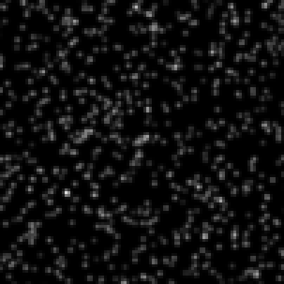
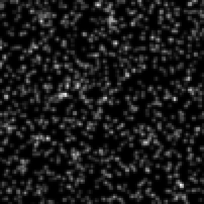
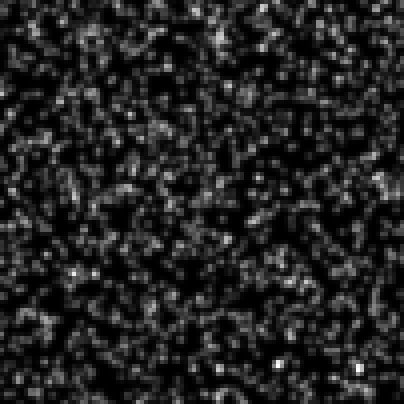
Figure 4: Detail of rendered 2D particle images for particles densities of 0.075, 0.125 and 0.175 (from left to right).

To quantitatively evaluate our approach and to compare different parameter settings we have generated synthetic data using the Johns Hopkins turbulence database (JHTDB) [49, 50]. The database provides a direct numerical simulation of isotropic turbulent flow in incompressible fluids. We can sample particles at arbitrary positions in the volume and track them over time. Additionally, we sample ground truth velocity flow vectors on a regular voxel grid.

Our setup consists of four cameras and particles rendered into a volume of $1024\times 512\times 352$ voxels. The cameras are arranged symmetrically with viewing angles of $\pm 35^{\circ}$ w.r.t. the $yz$-plane of the volume and $\pm 18^{\circ}$ w.r.t. the $xz$-plane. Camera images have a resolution of $1500\times 800$ pixels, where a pixel is approximately the size of a voxel. In this evaluation the maximum magnitude between two time steps is 4.8 voxels.

3D particles are rendered to the image planes as Gaussian blobs with $\sigma=1$ and intensity varying between 0.3 and 1, where the same intensity is used in all four cameras. We test different particle densities from $0.075$ to $0.2$ particles per pixel (ppp). A density of $0.1$ leads to a density of $\approx\frac{3}{10000}$ particles per voxel. Exemplary renderings for particle densities of $0.075$, $0.125$ and $0.175$ are shown in Figure 4.

We compare our method to [17] and test different particle densities and parameter settings. Our main evaluation criterion is the average endpoint error (AEE) of our estimated flow vectors, measured in voxels w.r.t. to the resolution of our test volume ($1024\times 512\times 352$). Standard parameter settings for our coarse-to-fine scheme are 9 pyramid levels and a pyramid scale factor of $0.95$ between adjacent pyramid levels. Note that larger velocity magnitudes would require more pyramid levels. We chose 10 warps and 20 inner iterations per pyramid level. Unless otherwise specified we use SSD as data cost. We also select our physically based regularizer $\operatorname{QRD_{\infty}}$ for our quantitative evaluation. According to [17], quadratic penalizing the gradient vectors of the flow, while enforcing a divergence-free vector field, performed better than other tested regularizers. For IPR we chose an intensity threshold of $\theta=0.04$, inner iterations $n_{steps}=40$ and 24 triangulation iterations, starting from a triangulation error $\epsilon=0.8$ and increasing it up to $\epsilon=2.0$. Note that for lower particle densities less iterations would already be sufficient. However, most particles will be triangulated already in earlier iterations, such that the additional runtime demand for more iterations becomes negligible. Flow vectors are estimated on every fourth voxel location per dimension, i.e. a $256\times 128\times 88$ voxel grid, and subsequently upscaled to $1024\times 512\times 352$ in order to be compared with the ground truth flow field. As shown in [17] flow estimation on the down-sampled grid can be performed with virtually no loss in accuracy, but with the benefit of faster computation and lower memory demands. In Figure 5 we visualize a single xy-slice (z=72) of the flow field for both, ground truth and our estimated flow, with standard settings at a particle density of $ppp=0.125$.

In addition to the quantitative evaluation we show qualitative results on test case D of the $4^{th}$ International PIV Challenge [51].

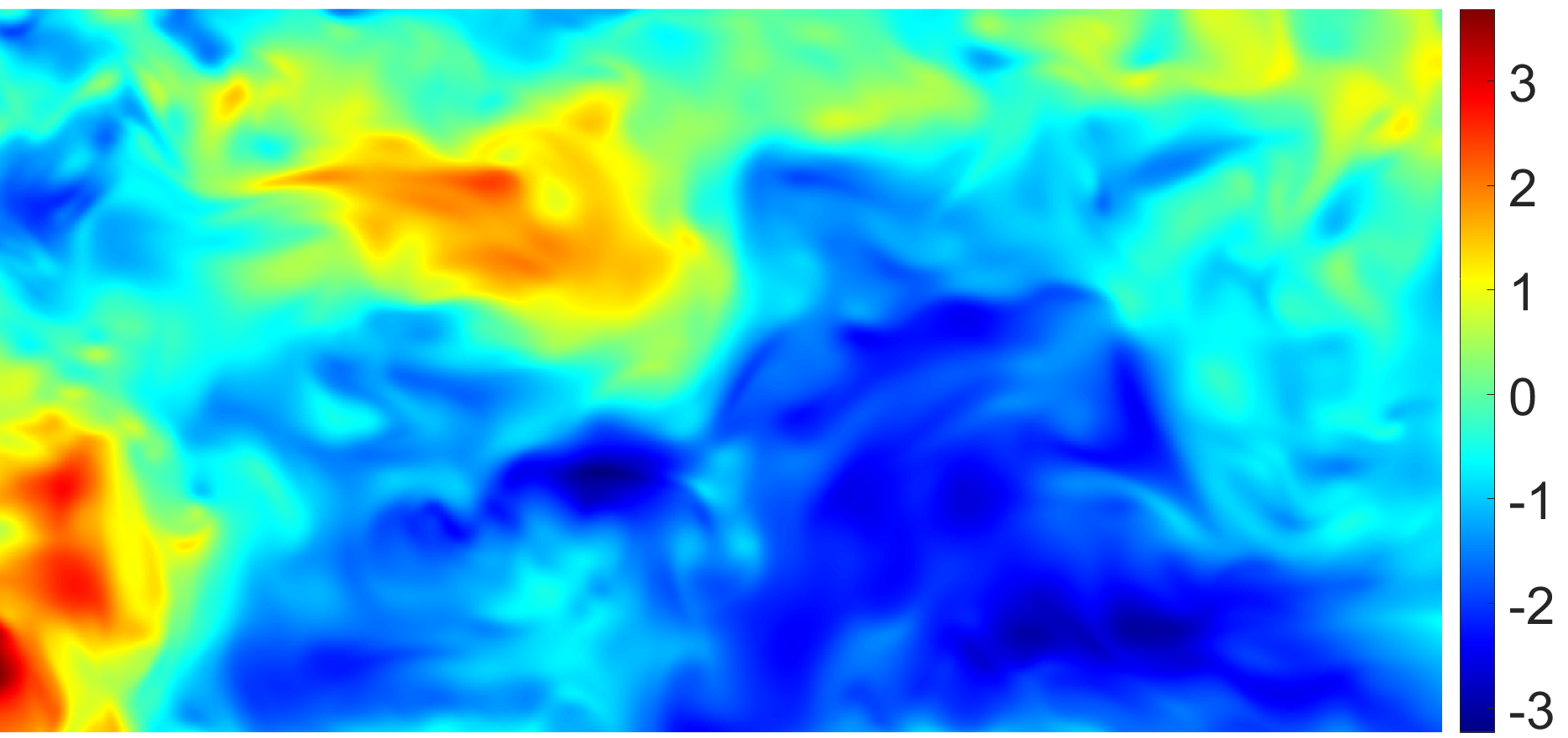
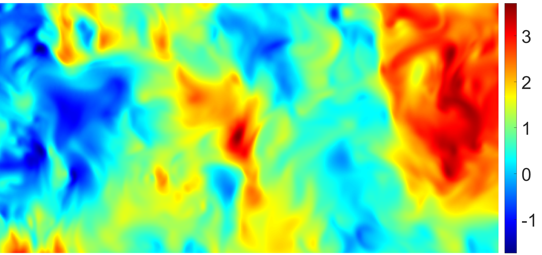
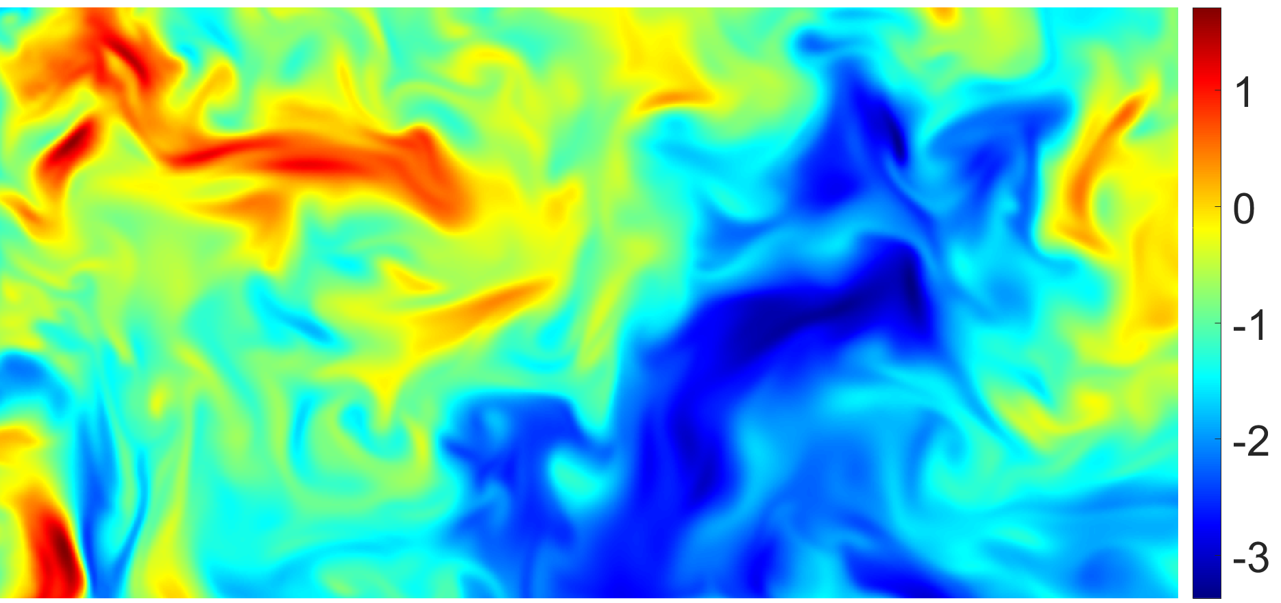
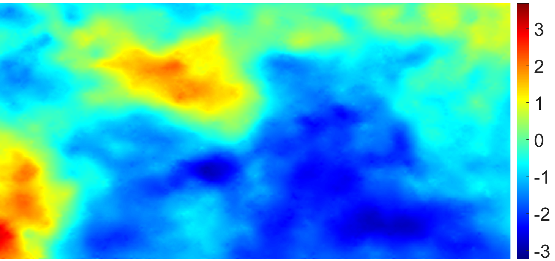
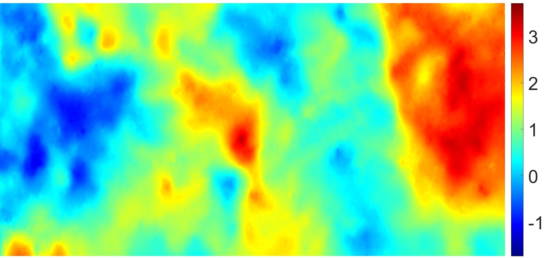
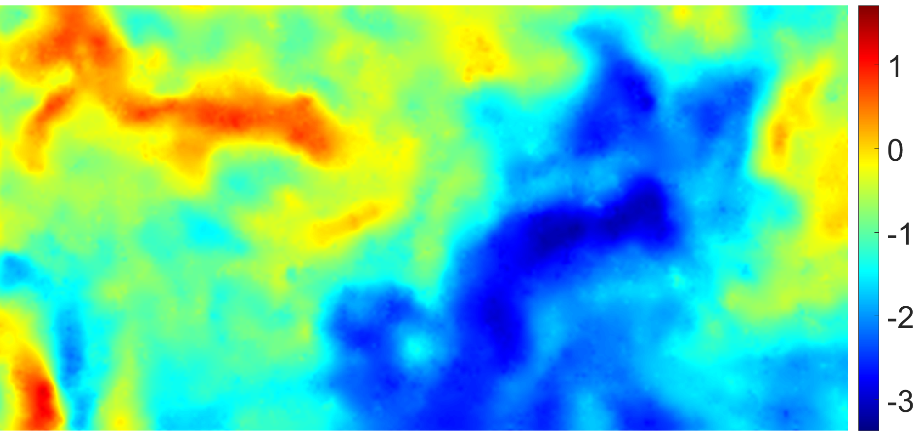
Figure 5: xy-slice of the flow in X-, Y- and Z-direction (left to right). Top: Ground truth. Bottom: Estimated flow for $ppp=0.125$.

3.1 3D Reconstruction & Particle Density

We start by comparing different initialization methods for various particle densities. Additional to our implementations of MART and IPR we also provide results for starting the flow reconstruction from the ground truth particle distributions. Following the naming convention of [51], we refer to this version as HACKER. In Table 2 we compare the estimated flow w.r.t. the AEE and furthermore show statistics on the particle reconstruction of time step 0, for both reconstruction techniques, MART and IPR. Reconstructed particles with no ground truth particle within a distance of 2 voxels are considered as ghost particles. As expected, assuming perfect particle reconstruction (HACKER) the flow estimation is still improving with higher particle densities. However, for increasing particle densities the reconstruction gets more ambiguous, as can be seen from the increased number of ghost particles, as well as missing particles for both MART and IPR. The numbers suggest that the current bottleneck of our pipeline can be found in the particle reconstruction. Furthermore, IPR consistently outperforms MART at all particle densities. Here, MART already starts to fail at lower particle densities while our IPR implementation yields results similar to HACKER up to a particle density of $0.15$.

Table 2: Comparison of different initialization methods (MART vs. IPR vs. HACKER).

Particle Density (ppp)		0.075	0.1	0.125	0.15	0.175	0.2
MART	Avg. endpoint error	0.2768	0.2817	0.2927	0.3119	0.3363	0.3500
	Undetected particles	1412	6283	13918	24141	37215	51190
		3.21%	10.7%	18.96%	27.41%	36.22%	43.59%
	Ghost particles	22852	44752	79356	107276	118476	129791
		51.89%	76.21%	108.11%	121.79%	115.29%	110.52%
	Avg. position error	1.681	1.672	1.663	1.654	1.647	1.638
IPR	Avg. endpoint error	0.2505	0.2388	0.2250	0.2260	0.2522	0.2950
	Undetected particles	18	24	35	582	14187	33936
		0.04%	0.04%	0.05%	0.66%	13.81%	28.90%
	Ghost particles	4	3	14	4344	107286	176176
		0.01%	0.01%	0.02%	4.93%	104.40%	150.01%
	Avg. position error	0.001	0.001	0.002	0.029	0.188	0.301
HACKER	Avg. endpoint error	0.2503	0.2382	0.2244	0.2229	0.2140	0.2068

3.2 Descriptor & Data Cost

We evaluate two different distance metrics for our sparse descriptor: sum of squared distances (SSD) and (negative) normalized cross-correlation (NCC). In addition to our spherical-shaped descriptor introduced in Section 2.2, we evaluate our approach with a descriptor based on a regular grid structure. A grid point is set at every second voxel position per dimension (i.e. -2,0,2) within a radius of 8, resulting in 257 grid points. Particles within a radius of $d=10.5$ are considered for the descriptor estimation. Here, we splat particles to $k=8$ regular grid points, and utilize $k=5$ for our standard layer based descriptor (with denser sampling closer to the descriptor center). The impact of these choices on the estimated flow vectors are summarized in Table 3 for various particle densities. Here both distance metrics, SSD and NCC, perform similarly well. Our spherical, layer based descriptor appears to work slightly, but also consistently, better than the descriptor based on the regular grid.

Table 3: Comparison of average endpoint error for different descriptors with IPR initialization.

Particle Density (ppp)		0.075	0.1	0.125	0.15
NCC	Layered spherical descriptor (331, d=21)	0.2492	0.2359	0.2270	0.2286
	Regular spherical grid (257, d=21)	0.2630	0.2498	0.2405	0.2431
SSD	Layered spherical descriptor (331, d=21)	0.2505	0.2388	0.2250	0.2260
	Regular spherical grid (257, d=21)	0.2643	0.2436	0.2362	0.2374

3.3 Comparison to Dense VolumeFlow

We compare our method to [17] where the data term is based on a high-resolution voxel grid, as obtained from MART. Additionally to MART reconstruction we also show results for IPR and HACKER, where particles were rendered into the volume by tri-linear interpolation to their nearest $2\times 2\times 2$ voxels. For the flow estimation we chose the recommended parameter set of [17]: SSD with IV size $13^{3}$, $\operatorname{QRD_{\infty}}$ and stepsize $h=4$. Average endpoint errors are shown in  Table 4 for different particle densities. Performance is slightly better than for our sparse descriptor variant, with the drawback that a memory demanding high resolution intensity volume is needed for the inherently sparse data. By adding more grid points to our descriptor (i.e. a grid point at every voxel location) we could effectively rebuild a dense matching approach with our sparse data. However, we opt for a more compact representation that allows faster computation and less memory requirements. Furthermore, our sparse descriptor can be adapted to any kind of similarity measure, where the use of numerical differentiation allows for a simple and quick evaluation. Here, it would be interesting to test also learned similarity functions, which could benefit from our compact representation [52, 53, 54].

Table 4: Average endpoint error of dense method for different initialization methods (MART vs. IPR vs. HACKER).

Particle Density (ppp)	0.075	0.1	0.125	0.15
MART	0.2470	0.2717	0.3144	0.3735
IPR	0.2266	0.2107	0.2001	0.2057
HACKER	0.2270	0.2112	0.2000	0.1923

3.4 PIV Challenge Data

Test case D of the $4^{th}$ International PIV Challenge [51] consists of 50 time steps of a volume of size $4096\times 512\times 352$ and a particle density of $0.1$. Unfortunately no ground truth is provided, however, we can visually compare our results to results stated in the challenge. In Figure 6 we show result of our method for snapshot 23 of the challenge, as well as the ground truth and the result of the top-performing method Shake-the-box (StB) [18]. The motion fields appear comparable, flow details are recovered. Note that our method uses only two frames to estimate the motion field, while StB relies on multiple time steps.

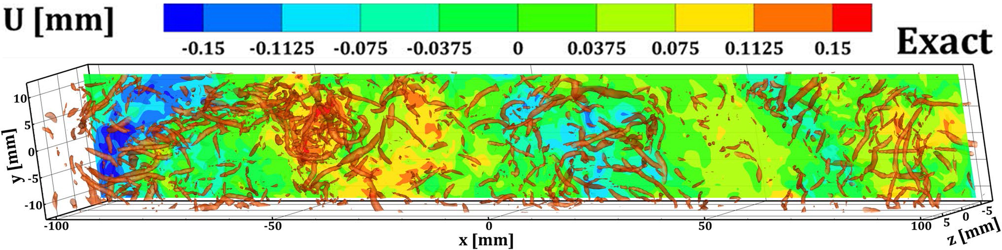
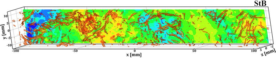
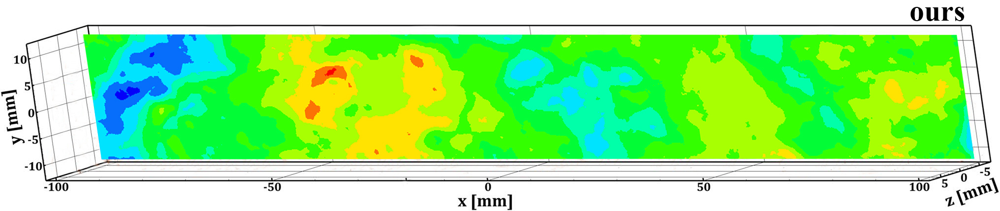
Figure 6: Visualization of xy-slice (z=-5.2mm) of snapshot 23 of the 4th International PIV Challenge [51] with discrete color coding to visually compare to results of participators of the challenge. Top: Ground truth (with additional visualization of vortices). Middle: StB [18], the best performing method of the challenge. Bottom: Our result. Images of ground truth and StB reproduced from [51].

4 Conclusion

Our method is based on and extends work of a conference publication [17]. In particular, we adopt their physically motivated regularization scheme and follow the same optimization methodology. We extend [17] with a novel, energy based IPR method that allows for more accurate and robust particle reconstructions. Relying on the quality of the 3D particle reconstruction, these advantages also affect the accuracy of our motion estimation technique, which before was based on the tomographic reconstruction model of MART. To further exploit sparsity of the directly reconstructed particles in the volume, we propose a novel sparse descriptor that can be constructed on-the-fly and possess a significantly lower memory footprint than a dense intensity volume, which is required in high resolution to deliver motion reconstructions of similar quality.

A current draw-back of our model is that the initially reconstructed particles are kept fixed and the mutual dependency of fluid motion and particle reconstruction is not considered. Hence, an interesting path to investigate in the future would be to combine particle reconstruction and flow estimation in a joint energy model.

References

- [1] K. Ohmi and H.-Y. Li, “Particle-tracking velocimetry with new algorithms,” Measurement Science and Technology, vol. 11, no. 6, p. 603, 2000.
- [2] R. Adrian and J. Westerweel, Particle Image Velocimetry. Cambridge University Press, 2011.
- [3] M. Raffel, C. E. Willert, S. Wereley, and J. Kompenhans, Particle image velocimetry: a practical guide. Springer, 2013.
- [4] G. E. Elsinga, F. Scarano, B. Wieneke, and B. W. Oudheusden, “Tomographic particle image velocimetry,” Experiments in Fluids, vol. 41, no. 6, 2006.
- [5] C. Atkinson and J. Soria, “An efficient simultaneous reconstruction technique for tomographic particle image velocimetry,” Experiments in Fluids, vol. 47, no. 4, 2009.
- [6] S. Discetti and T. Astarita, “Fast 3D PIV with direct sparse cross-correlations,” Experiments in Fluids, vol. 53, no. 5, 2012.
- [7] F. Champagnat, P. Cornic, A. Cheminet, B. Leclaire, G. L. Besnerais, and A. Plyer, “Tomographic piv: particles versus blobs,” Measurement Science and Technology, vol. 25, no. 8, p. 084002, 2014.
- [8] F. Champagnat, A. Plyer, G. Le Besnerais, B. Leclaire, S. Davoust, and Y. Le Sant, “Fast and accurate PIV computation using highly parallel iterative correlation maximization,” Experiments in Fluids, vol. 50, no. 4, p. 1169, 2011.
- [9] R. Yegavian, B. Leclaire, F. Champagnat, C. Illoul, and G. Losfeld, “Lucas-kanade fluid trajectories for time-resolved piv,” Measurement Science and Technology, vol. 27, no. 8, p. 084004, 2016.
- [10] B. D. Lucas and T. Kanade, “An iterative image registration technique with an application to stereo vision,” in Proceedings of the 7th International Joint Conference on Artificial Intelligence - Volume 2, IJCAI’81, (San Francisco, CA, USA), pp. 674–679, Morgan Kaufmann Publishers Inc., 1981.
- [11] B. K. P. Horn and B. G. Schunck, “Determining optical flow,” Artificial Intelligence, vol. 17, 1981.
- [12] T. Brox, A. Bruhn, N. Papenberg, and J. Weickert, “High accuracy optical flow estimation based on a theory for warping,” in ECCV 2004, pp. 25–36, Springer.
- [13] C. Zach, T. Pock, and H. Bischof, “A duality based approach for realtime TV-L1 optical flow,” DAGM 2007.
- [14] M. Werlberger, T. Pock, and H. Bischof, “Motion estimation with non-local total variation regularization,” in CVPR 2010, pp. 2464–2471, .
- [15] D. Heitz, E. Mémin, and C. Schnörr, “Variational fluid flow measurements from image sequences: synopsis and perspectives,” Experiments in Fluids, vol. 48, no. 3, 2010.
- [16] L. Alvarez, C. Castaño, M. García, K. Krissian, L. Mazorra, A. Salgado, and J. Sánchez, “A new energy-based method for 3d motion estimation of incompressible PIV flows,” Computer Vision and Image Understanding, vol. 113, no. 7, 2009.
- [17] K. Lasinger, C. Vogel, and K. Schindler, “Volumetric flow estimation for incompressible fluids using the stationary stokes equations,” ICCV 2017.
- [18] D. Schanz, S. Gesemann, and A. Schröder, “Shake-The-Box: Lagrangian particle tracking at high particle image densities,” Experiments in Fluids, vol. 57, no. 5, 2016.
- [19] S. Gesemann, F. Huhn, D. Schanz, and A. Schröder, “From noisy particle tracks to velocity, acceleration and pressure fields using B-splines and penalties,” Int’l Symp. on Applications of Laser Techniques to Fluid Mechanics, 2016.
- [20] J. F. Schneiders and F. Scarano, “Dense velocity reconstruction from tomographic PTV with material derivatives,” Experiments in Fluids, vol. 57, no. 9, 2016.
- [21] D. G. Lowe, “Distinctive image features from scale-invariant keypoints,” IJCV, vol. 60, no. 2, pp. 91–110, 2004.
- [22] N. Dalal and B. Triggs, “Histograms of oriented gradients for human detection,” in CVPR 2005, vol. 1, pp. 886–893, IEEE.
- [23] K. Mikolajczyk and C. Schmid, “A performance evaluation of local descriptors,” PAMI, vol. 27, pp. 1615–1630, Oct. 2005.
- [24] R. Zabih and J. Woodfill, “Non-parametric local transforms for computing visual correspondence,” in Proceedings of the Third European Conference on Computer Vision (Vol. II), ECCV 1994, (Secaucus, NJ, USA), pp. 151–158, Springer-Verlag New York, Inc.
- [25] C. Liu, J. Yuen, and A. Torralba, “Sift flow: Dense correspondence across scenes and its applications,” IEEE transactions on pattern analysis and machine intelligence, vol. 33, no. 5, pp. 978–994, 2011.
- [26] A. Schröder, R. Geisler, K. Staack, G. E. Elsinga, F. Scarano, B. Wieneke, A. Henning, C. Poelma, and J. Westerweel, “Eulerian and lagrangian views of a turbulent boundary layer flow using time-resolved tomographic piv,” Experiments in Fluids, vol. 50, pp. 1071–1091, Apr 2011.
- [27] B. Wieneke, “Iterative reconstruction of volumetric particle distribution,” Measurement Science & Technology, vol. 24, no. 2, 2013.
- [28] B. Wieneke, “Volume self-calibration for 3d particle image velocimetry,” Experiments in fluids, vol. 45, no. 4, pp. 549–556, 2008.
- [29] D. Schanz, S. Gesemann, A. Schröder, B. Wieneke, and M. Novara, “Non-uniform optical transfer functions in particle imaging: calibration and application to tomographic reconstruction,” Measurement Science & Technology, vol. 24, no. 2, 2012.
- [30] R. Gordon, R. Bender, and G. T. Herman, “Algebraic reconstruction techniques (ART) for three-dimensional electron microscopy and x-ray photography,” Journal of Theoretical Biology, vol. 29, pp. 471–481, 1970.
- [31] S. Discetti, A. Natale, and T. Astarita, “Spatial filtering improved tomographic PIV,” Experiments in Fluids, vol. 54, no. 4, 2013.
- [32] S. Petra, A. Schröder, and C. Schnörr, “3D tomography from few projections in experimental fluid dynamics,” in Imaging Measurement Methods for Flow Analysis: Results of the DFG Priority Programme 1147, 2009.
- [33] J. Bolte, S. Sabach, and M. Teboulle, “Proximal alternating linearized minimization for nonconvex and nonsmooth problems,” Mathematical Programming, vol. 146, no. 1, pp. 459–494, 2014.
- [34] T. Pock and S. Sabach, “Inertial proximal alternating linearized minimization (iPALM) for nonconvex and nonsmooth problems,” SIAM J Imaging Sci, vol. 9, no. 4, pp. 1756–1787, 2016.
- [35] H. Attouch, J. Bolte, and B. F. Svaiter, “Convergence of descent methods for semi-algebraic and tame problems: proximal algorithms, forward–backward splitting, and regularized Gauss–Seidel methods,” Mathematical Programming, vol. 137, no. 1, pp. 91–129, 2013.
- [36] J. Bolte, A. Daniilidis, and A. Lewis, “The Lojasiewicz inequality for nonsmooth subanalytic functions with applications to subgradient dynamical systems,” SIAM J Optimiz, vol. 17, no. 4, pp. 1205–1223, 2007.
- [37] D. P. Bertsekas and J. N. Tsitsiklis, Parallel and Distributed Computation: Numerical Methods. Prentice-Hall, 1989.
- [38] A. Beck and M. Teboulle, “A fast iterative shrinkage-thresholding algorithm for linear inverse problems,” SIAM J Imaging Sci, vol. 2, no. 1, pp. 183–202, 2009.
- [39] A. Frome, D. Huber, R. Kolluri, T. Bülow, and J. Malik, “Recognizing objects in range data using regional point descriptors,” Computer vision-ECCV 2004, pp. 224–237, 2004.
- [40] P. Scovanner, S. Ali, and M. Shah, “A 3-dimensional sift descriptor and its application to action recognition,” in Proceedings of the 15th ACM International Conference on Multimedia, MM ’07, (New York, NY, USA), pp. 357–360, ACM, 2007.
- [41] Y. H. Le, U. Kurkure, and I. A. Kakadiaris, “3d dense local point descriptors for mouse brain gene expression images,” Computerized Medical Imaging and Graphics, vol. 38, no. 5, pp. 326 – 336, 2014.
- [42] J. H. Friedman, J. L. Bentley, and R. A. Finkel, “An algorithm for finding best matches in logarithmic expected time,” ACM Trans. Math. Softw., vol. 3, pp. 209–226, Sept. 1977.
- [43] M. Muja and D. G. Lowe, “Scalable nearest neighbor algorithms for high dimensional data,” PAMI, vol. 36, 2014.
- [44] A. Chambolle and T. Pock, “A first-order primal-dual algorithm for convex problems with applications to imaging,” JMIV, vol. 40, no. 1, 2011.
- [45] J. J. Monaghan, “Smoothed particle hydrodynamics,” Reports on Progress in Physics, vol. 68, no. 8, p. 1703, 2005.
- [46] B. Adams, M. Pauly, R. Keiser, and L. J. Guibas, “Adaptively sampled particle fluids,” ACM SIGGRAPH 2007.
- [47] C. Vogel, S. Roth, and K. Schindler, “An evaluation of data costs for optical flow,” GCPR 2013.
- [48] L. I. Rudin, S. Osher, and E. Fatemi, “Nonlinear total variation based noise removal algorithms,” PhysḊ, vol. 60, no. 1-4, 1992.
- [49] Y. Li, E. Perlman, M. Wan, Y. Yang, C. Meneveau, R. Burns, S. Chen, A. Szalay, and G. Eyink, “A public turbulence database cluster and applications to study Lagrangian evolution of velocity increments in turbulence,” Journal of Turbulence, vol. 9, 2008.
- [50] E. Perlman, R. Burns, Y. Li, and C. Meneveau, “Data exploration of turbulence simulations using a database cluster,” in ACM/IEEE Conf. on Supercomputing, 2007.
- [51] C. J. Kähler, T. Astarita, P. P. Vlachos, J. Sakakibara, R. Hain, S. Discetti, R. La Foy, and C. Cierpka, “Main results of the 4th International PIV Challenge,” Experiments in Fluids, vol. 57, no. 6, 2016.
- [52] K. M. Yi, E. Trulls, V. Lepetit, and P. Fua, “LIFT: Learned Invariant Feature Transform,” in Proceedings of the European Conference on Computer Vision, 2016.
- [53] J. Zbontar and Y. LeCun, “Stereo matching by training a convolutional neural network to compare image patches,” Journal of Machine Learning Research, vol. 17, no. 1-32, p. 2, 2016.
- [54] M. Khoury, Q.-Y. Zhou, and V. Koltun, “Learning compact geometric features,” in Proceedings of the IEEE Conference on Computer Vision and Pattern Recognition, pp. 153–161, 2017.