Semantic Edge Detection with Diverse Deep Supervision

Abstract

Semantic edge detection (SED), which aims at jointly extracting edges as well as their category information, has far-reaching applications in domains such as semantic segmentation, object proposal generation, and object recognition. SED naturally requires achieving two distinct supervision targets: locating fine detailed edges and identifying high-level semantics. Our motivation comes from the hypothesis that such distinct targets prevent state-of-the-art SED methods from effectively using deep supervision to improve results. To this end, we propose a novel fully convolutional neural network using diverse deep supervision (DDS) within a multi-task framework where bottom layers aim at generating category-agnostic edges, while top layers are responsible for the detection of category-aware semantic edges. To overcome the hypothesized supervision challenge, a novel information converter unit is introduced, whose effectiveness has been extensively evaluated on SBD and Cityscapes datasets.

1 Introduction

The aim of classical edge detection is to detect edges and object boundaries in natural images. It is category-agnostic, in that object categories need not be recognized. Classical edge detection can be viewed as a pixel-wise binary classification problem, whose objective is to classify each pixel as belonging to either the class indicating an edge, or the class indicating a non-edge. In this paper, we consider more practical scenarios of semantic edge detection (SED), which jointly achieves edge detection and edge category recognition within an image. SED Hariharan et al. (2011); Yu et al. (2017); Maninis et al. (2017); Bertasius et al. (2015b) is an active computer vision research topic due to its wide-ranging applications, including object proposal generation Bertasius et al. (2015b), occlusion and depth reasoning Amer et al. (2015); Bian et al. (2021), 3D reconstruction Shan et al. (2014), object detection Ferrari et al. (2008, 2010), and image-based localization Ramalingam et al. (2010).

In the past several years, deep convolutional neural networks (DCNNs) reign undisputed as the new de-facto method for category-agnostic edge detection Xie & Tu (2015, 2017); Liu et al. (2017, 2019); Hu et al. (2018), where near human-level performance has been achieved. However, deep learning for category-aware SED, which jointly detects visually salient edges as well as recognizing their categories, has not yet witnessed such vast popularity. Hariharan et al. Hariharan et al. (2011) first combined generic object detectors with bottom-up edges to recognize semantic edges. Yang et al. Yang et al. (2016) proposed a fully convolutional encoder-decoder network to detect object contours but without recognizing specific categories. More recently, CASENet Yu et al. (2017) introduces a skip-layer structure to enrich the top-layer category-aware edge activation with bottom-layer features, improving previous state-of-the-art methods with a significant margin. However, CASENet imposes supervision only at the Side-5 and final fused classification and uses feature maps from Side-1 $\sim$ Side-3 without deep supervision. After unsuccessfully trying various ways of adding deep supervision, CASENet claims that imposing deep supervision at bottom network sides (Side-1 $\sim$ Side-4) is unnecessary. This conclusion has also been widely accepted by recent SED works Yu et al. (2018); Acuna et al. (2019); Hu et al. (2019).

(a) Original image

(b) Ground truth

(c) Color codes

(d) Side-1

(e) Side-2

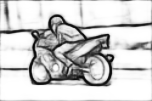
(f) Side-3

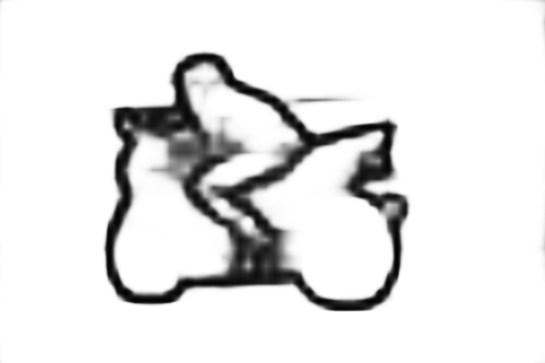
(g) Side-4

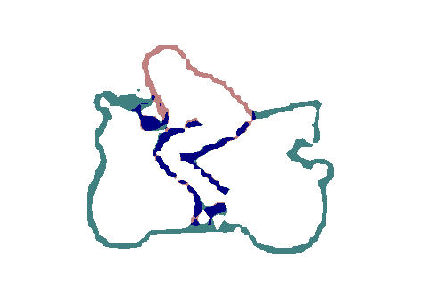
(h) Side-5

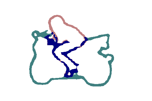
(i) DDS

Figure 1: An example of our DDS algorithm. (a) shows the original image from the SBD dataset Hariharan et al. (2011). (b)-(c) show its semantic edge map and corresponding color codes. (d)-(g) display category-agnostic edges from Side-1 $\sim$ Side-4. (h)-(i) show semantic edges of Side-5 and DDS (DDS-R) output, respectively.

SED naturally requires achieving two distinct supervision targets: i) locating fine detailed edges by capturing discontinuity among image regions, mainly using low-level features; and ii) identifying abstracted high-level semantics by summarizing different appearance variations of the target categories. While it may be intuitive and straightforward to impose category-agnostic edge supervision at bottom network sides for low-level edge details and impose category-aware edge supervision at top sides for semantic classification, directly doing this as in CASENet Yu et al. (2017) even degrades the performance compared with directly learning semantic edges without deep supervision or category-agnostic edge guidance. We hypothesize that distinct supervision targets prevent state-of-the-art SED methods Yu et al. (2017, 2018); Acuna et al. (2019); Hu et al. (2019) from successfully applying deep supervision Lee et al. (2015). Specifically, we observe that the success stories of deep supervision, including image categorization Szegedy et al. (2015), object detection Lin et al. (2020), visual tracking Wang et al. (2015), and category-agnostic edge detection Xie & Tu (2017); Liu et al. (2017), usually adopt the same type of supervision for all network sides. In contrast, CASENet directly imposes distinct supervision targets to bottom and top network sides. Therefore, we consider achieving such distinct supervision using some buffers, i.e., in an indirect manner, to prevent the backbone network from being directly influenced by distinct targets.

In this paper, we propose a diverse deep supervision (DDS) method, which employs deep supervision with different loss functions for high-level and low-level feature learning, as shown in Fig. 2(b). To this end, we propose an information converter unit to change the backbone DCNN features into different representations, for training category-agnostic or semantic edges, respectively. Hence, information converters act as buffers, making distinct supervision targets indirectly affect top and bottom convolution (i.e., conv layers. The existence of information converters separates the information content in conv layers by assigning unique sets of parameters and imposing separate losses to each network side. This makes a single backbone network be effectively trained end-to-end towards different targets. An example of DDS is shown in Fig. 1. The bottom sides of the neural network help Side-5 to find fine details, thus making the final fused semantic edges (Fig. 1(i)) smoother than those coming from Side-5 (Fig. 1(h)).

In summary, our main contributions include:

• We analyze the reason why state-of-the-art SED methods cannot apply deep supervision to improve results, i.e., due to the distinct supervision targets in SED (Section 3).

• We propose a new SED method, called diverse deep supervision (DDS), which uses information converters to separate the information content in backbone conv layers and thus achieve distinct supervision in an indirect manner (Section 4).

• We provide detailed ablation studies to further understand the proposed method (Section 5.2).

We extensively evaluate DDS on SBD Hariharan et al. (2011) and Cityscapes Cordts et al. (2016) datasets. DDS achieves state-of-the-art performance, demonstrating the reasonability of our analyses and thus opening up a new path for future SED research.

2 Related Work

An exhaustive review of the abundant literature on this topic is out of the scope of this paper. Instead, we first summarize the most important threads of research to solve the problem of classical category-agnostic edge detection, followed by the discussions of deep learning-based approaches, semantic edge detection (SED), and the technique of deep supervision.

Classical category-agnostic edge detection. Edge detection is conventionally solved by designing various filters (e.g., Sobel Sobel (1970) and Canny Canny (1986)) or complex models Mafi et al. (2018); Shui & Wang (2017) to detect pixels with highest gradients in their local neighborhoods Trahanias & Venetsanopoulos (1993); Hardie & Boncelet (1995); Henstock & Chelberg (1996). To the best of our knowledge, Konishi et al. Konishi et al. (2003) proposed the first data-driven edge detector in which, unlike previous model based approaches, edge detection was posed as statistical inferences. Pb features consisting of brightness, color and texture are used in  Martin et al. (2004) to obtain the posterior probability of each boundary point. Pb is further extended to gPb Arbeláez et al. (2011) by computing local cues from multi-scale and globalizing them through spectral clustering. Sketch tokens are learned from hand-drawn sketches for contour detection Lim et al. (2013), while random decision forests are employed in Dollár & Zitnick (2015) to learn the local structure of edge patches, delivering competitive results among non-deep-learning approaches.

Deep category-agnostic edge detection. The number of success stories of machine learning has seen an all-time rise across many computer vision tasks recently. The unifying idea is deep learning which utilizes neural networks with many hidden layers aimed at learning complex feature representations from raw data Chan et al. (2015); Tang et al. (2017); Liu et al. (2018). Motivated by this, deep learning based methods have made vast inroads into edge detection as well Wang et al. (2019); Deng et al. (2018); Yang et al. (2017). Ganin et al. Ganin & Lempitsky (2014) applied deep neural network for edge detection using a dictionary learning and nearest neighbor algorithm. DeepEdge Bertasius et al. (2015a) first extracts candidate contour points and then classifies these candidates. HFL Bertasius et al. (2015b) uses SE Dollár & Zitnick (2015) to generate candidate edge points in contrast to Canny Canny (1986) used in DeepEdge. Compared with DeepEdge which has to process input patches for every candidate point, HFL turns out to be more computationally feasible as the input image is only fed into the network once. DeepContour Shen et al. (2015) partitions edge data into subclasses and fits each subclass using different model parameters. Xie et al. Xie & Tu (2015, 2017) leveraged deeply-supervised nets to build a fully convolutional network for image-to-image prediction. Their deep model, known as HED, fuses the information from the bottom and top conv layers. Kokkinos Kokkinos (2016) proposed some training strategies to retrain HED. Liu et al. Liu et al. (2017, 2019) introduced the first real-time edge detector, which achieves higher F-measure scores than average human annotators on the popular BSDS500 dataset Arbeláez et al. (2011).

Semantic edge detection. By virtue of their strong capacity for semantic representation learning, DCNNs based edge detectors tend to generate high responses at object boundary locations, e.g., Fig. 1 (d)-(g). This has inspired research on simultaneously detecting edge pixels and classifying them based on associations with one or more object categories. This so-called “category-aware” edge detection is highly beneficial to a wide range of vision tasks including object recognition, stereo vision, semantic segmentation, and object proposal generation.

Hariharan et al. Hariharan et al. (2011) proposed the first principled way of combining generic object detectors with bottom-up contours to detect semantic edges. Yang et al. Yang et al. (2016) proposed a fully convolutional encoder-decoder network for object contour detection. HFL Bertasius et al. (2015b) produces category-agnostic binary edges and assigns class labels to all boundary points using deep semantic segmentation networks. Maninis et al. Maninis et al. (2017) coupled their convolutional oriented boundaries (COB) with semantic segmentation generated by dilated convolutions Yu & Koltun (2016) to obtain semantic edges. A weakly supervised learning strategy is introduced in Khoreva et al. (2016), where bounding box annotations alone are sufficient to produce high-quality object boundaries without any object-specific annotations. Gated-SCNN Takikawa et al. (2019) converts the semantic edge representation from different ResNet layers to a representation suitable for segmentation, improving semantic segmentation substantially.

Yu et al. Yu et al. (2017) proposed a novel network, CASENet, which has pushed SED performance to a new state-of-the-art. In their architecture, low-level features are only used to augment top classifications. After several failed experiments, they reported that imposing deep supervision at bottom sides is unnecessary for SED. More recently, Yu et al. Yu et al. (2018) introduced a new training approach, SEAL, to train CASENet Yu et al. (2017). This approach can simultaneously align ground-truth edges and learn semantic edge detectors. However, the training of SEAL is very time-consuming due to the heavy CPU computation load. For example, it needs over 16 days to train CASENet on the SBD dataset Hariharan et al. (2011), despite that we have used a powerful CPU (Intel Xeon(R) CPU E5-2683 v3 @ 2.00GHz $\times$ 56). Hu et al. Hu et al. (2019) proposed a novel dynamic feature fusion (DFF) strategy to assign different fusion weights for different input images and locations adptively in the fusion of multi-scale DCNN features. Acuna et al. Acuna et al. (2019) focused on semantic thinning edge alignment learning (STEAL). They presented a simple new layer and loss to train CASENet Yu et al. (2017), so that they can learn sharp and precise semantic boundaries. However, all above methods give up applying deep supervision to bottom layers due to the distinct supervision targets in SED. In this work, we aim to solve this problem, so our method is compatible with previous methods, including SEAL Yu et al. (2018), DFF Hu et al. (2019), and STEAL Acuna et al. (2019).

Deep supervision. Deep supervision has been demonstrated to be effective in many vision and learning tasks such as image classification Lee et al. (2015); Szegedy et al. (2015), object detection Lin et al. (2020, 2017); Liu et al. (2016), visual tracking Wang et al. (2015), category-agnostic edge detection Xie & Tu (2017); Liu et al. (2017), salient object detection Hou et al. (2019), and so on. Theoretically, the bottom layers of deep networks can learn discriminative features so that classification/regression at top layers is easier. In practice, one can explicitly influence the hidden layer weight/filter update process to favor highly discriminative feature maps using deep supervision. However, traditional deep supervision usually adopts the same type of supervision at all layers, so it may be suboptimal for SED to directly apply distinct supervision of category-agnostic and category-aware edges to bottom and top network sides, respectively. In the following sections, we will first analyze the problem of distinct supervision targets of SED and then introduce a new semantic edge detector with successful diverse deep supervision.

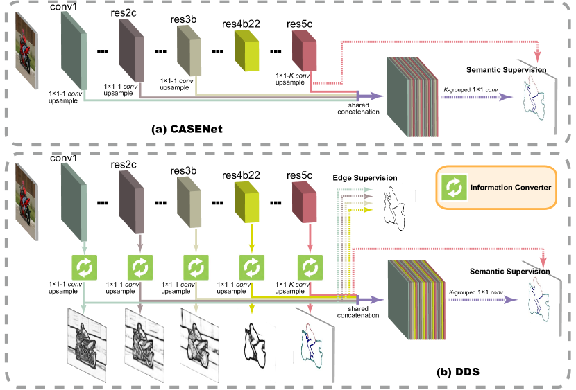
Figure 2: A comparison between two SED models: CASENet Yu et al. (2017) and our DDS. CASENet only adds top supervision on the Side-5 activation, and the authors claimed that deep supervision was not necessary in their architecture. However, our proposed DDS network adds deep supervision at all network sides. Note that information converters are crucial for resolving the distinct supervision targets of category-agnostic and category-aware edges.

3 Distinct Supervision Targets in SED

Before expounding the proposed method, we first analyze the problem caused by the distinct supervision targets of SED.

3.1 A Typical Deep Model for SED

To introduce previous attempts for using deep supervision in SED, without loss of generality, we take a typical deep model as an example, i.e., CASENet Yu et al. (2017). As shown in Fig. 2(a), this typical model is built on the well-known backbone network of ResNet He et al. (2016). It connects a $1\times 1$ conv layer after each of Side-1 $\sim$ Side-3 to produce a single-channel feature map $F^{(m)}$. The top Side-5 is connected to a $1\times 1$ conv layer to output $K$-channel class activation map $A^{(5)}=\{A_{1}^{(5)},A_{2}^{(5)},\cdots,A_{K}^{(5)}\}$, where $K$ is the number of categories. Then, the shared concatenation replicates bottom features $F^{(m)}$ to separately concatenate each channel of the class activation map:

$$F^{f}=\{F^{(1)},F^{(2)},F^{(3)},A_{1}^{(5)},\cdots,F^{(1)},F^{(2)},F^{(3)},A_{K}^{(5)}\}.$$ (1)

Next, a $K$-grouped $1\times 1$ conv is performed on $F^{f}$ to generate a semantic edge map with $K$ channels, in which the $k$-th channel represents the edge map for the $k$-th category. Other SED models Yu et al. (2018); Hu et al. (2019) have similar network designs.

3.2 Discussion

Previous SED models Yu et al. (2017, 2018); Bertasius et al. (2015b); Hu et al. (2019) only impose supervision on Side-5 and the final fused activation. In CASENet, the authors have tried several deeply supervised architectures. They first separately used all of Side-1 $\sim$ Side-5 for SED, with each side connected with a semantic classification loss. The evaluation results are even worse than the basic architecture that directly applies $1\times 1$ convolution at Side-5 to obtain semantic edges. It is widely accepted that the bottom layers of DCNNs contain low-level, less-semantic features such as local edges, which are less effective for semantic classification because semantic category recognition needs abstracted high-level features that mainly appear in the top layers of neural networks. Thus, they would obtain poor classification results at bottom sides. Unsurprisingly, simply connecting each low-level feature layer and high-level feature layer with a classification loss and deep supervision for SED results in a clear performance drop.

Yu et al. Yu et al. (2017) also attempted to impose deep supervision of binary edges at Side-1 $\sim$ Side-3 in CASENet but observed divergence in the semantic classification at Side-5. Here, we provide an intuitive and reasonable explanation for this phenomenon. With the top supervision of semantic edges, the top layers of the network will be supervised to learn abstracted high-level semantics that can summarize different appearance variations of object categories. Since bottom layers are the bases of top layers for the representation power of DCNNs, bottom layers will be supervised to serve top layers for obtaining high-level semantics through back propagation. Conversely, with bottom supervision of category-agnostic edges, bottom layers are taught to focus on distinction between edges and non-edges, rather than visual representations for semantic classification. Hence, bottom layers have two conflict supervision targets. Compared to traditional deep supervision applications that usually adopt the same type of supervision, we believe that such distinct supervision targets of SED lead to the failure of previous attempts to apply deep supervision for SED. Our motivation of this work comes from this hypothesis by trying to resolve such distinct supervision targets.

Note that Side-4 is not used in CASENet. We think that it is a naive way to alleviate the supervision conflicts by regarding the whole res4 block as a buffer unit between bottom and top sides. Indeed, when adding Side-4 to CASENet (see Section 5.2), the new model (CASENet +S4) achieves a 70.9% mean F-measure, compared to 71.4% of original CASENet. This suggests that our hypothesis about the buffer function of res4 block may be reasonable. Moreover, the classical $1\times 1$ conv layer after each side Xie & Tu (2017); Yu et al. (2017) is too weak to buffer the conflicts. We therefore propose an information converter unit to try to separate the information content in the backbone layers by assigning unique sets of parameters and imposing separate losses to each network side. In this way, we tackle the distinct supervision targets of SED in an indirect manner, rather than the previous direct manner.

4 Methodology

Intuitively, by employing different but “appropriate” ground truths for bottom and top sides, the learned intermediate representations of the different levels may contain complementary information. However, directly imposing deep supervision does not seem to be beneficial. In this section, we propose a new network architecture for the complementary learning of bottom and top sides for SED.

4.1 Diverse Deep Supervision

Based on the above discussion, we hypothesize that the bottom sides of neural networks may not be directly beneficial to SED. However, we still believe that bottom sides encode fine details complementary to the top side (Side-5). With appropriate architecture re-design, maybe they can be used for category-agnostic edge detection to improve the localization accuracy of semantic edges generated by the top side. To this end, we design a novel information converter to assist low-level feature learning, making it consistent with high-level feature learning. This is essential as this enables bottom layers to learn find-grained details and serve top layers to favor highly discriminative features simultaneously.

Our proposed network architecture is presented in Fig. 2(b). We follow CASENet to use ResNet He et al. (2016) as our backbone network. After each information converter (Section 4.2) in Side-1 $\sim$ Side-4, we connect a $1\times 1$ conv layer with a single output channel to produce an edge response map. These predicted maps are then upsampled to the original image size using bilinear interpolation. These side-outputs are supervised by binary category-agnostic edges. We perform $K$-channel $1\times 1$ convolution on Side-5 to obtain semantic edges, where each channel represents the binary edge map of one category. We adopt the same upsampling operation as for Side-1 $\sim$ Side-4. Semantic edges are used to supervise the training of Side-5.

We denote the produced binary edge maps from Side-1 $\sim$ Side-4 as $E=\{E^{(1)},E^{(2)},E^{(3)},E^{(4)}\}$. The semantic edge map from Side-5 is still represented by $A^{(5)}$. A shared concatenation is then performed to obtain the stacked edge activation map:

$$E^{f}=\{E,A_{1}^{(5)},E,A_{2}^{(5)},E,A_{3}^{(5)},\cdots,E,A_{K}^{(5)}\}.$$ (2)

Note that $E^{f}$ is a stacked edge activation map, while $F^{f}$ in CASENet is a stacked feature map. Finally, we apply $K$-grouped $1\times 1$ convolution on $E^{f}$ to generate the fused semantic edges. The fused edges are supervised by the ground truth of the semantic edges. As shown in HED Xie & Tu (2017), the $1\times 1$ convolution can fuse the edges from bottom and top sides well.

4.2 Information Converter

From the above analyses, the core for improving SED is the existence of the information converter. In this paper, we try a simple design for information converter to validate our hypothesis. Recently, residual networks have been proved to be easier to optimize than plain networks He et al. (2016). The residual learning operation is embodied by a shortcut connection and element-wise addition. We describe a residual conv block in Fig. 3, which consists of two alternatively connected ReLU and conv layers, and the output of the first ReLU layer is added to the output of the last conv layer. Our proposed information converter combines two residual modules and is connected to each side of the DDS network to transform the learned representation into the proper form. This operation is expected to avoid the conflicts caused by the discrepancy in different losses.

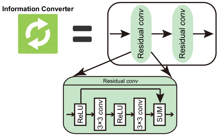
Figure 3: Schematic of our information converter unit (illustrated in the orange box in Fig. 2).

The top supervision of semantic edges will guide top layers in learning semantic features, while the bottom supervision of category-agnostic edges will guide bottom layers in learning category-agnostic features. Hence, bottom layers would have two distinct supervision through back propagation if the distinct supervision is directly imposed as discussed in Section 3. Our information converters can separate the information content in the backbone layers by assigning unique sets of parameters and imposing separate losses to each network side, playing a buffering role. In this way, the distinct supervision targets are imposed to the backbone network in an indirect manner, rather than the previous direct manner Yu et al. (2017, 2018); Bertasius et al. (2015b); Hu et al. (2019). Note that this paper mainly claims the importance of the existence of the information converter, not its specific format, so we only adopt a simple design. In the experimental part, we will demonstrate different designs for the information converter achieve similar performance.

Our proposed network can successfully combine the fine details from bottom sides and the semantic information from top sides. Our experimental results demonstrate that this method solves the problem of conflicts caused by diverse deep supervision. Unlike CASENet, our semantic classification at Side-5 can be well optimized without any divergence. The produced binary edges from bottom sides help Side-5 make up fine details. Thus, the final fused semantic edges can achieve better localization quality.

We use binary edges of single pixel width to supervise Side-1 $\sim$ Side-4 and thick semantic boundaries to supervise Side-5 and the final fused edges. One pixel is viewed as a binary edge if it belongs to the semantic boundaries of any category. We obtain thick semantic boundaries by seeking the difference between a pixel and its neighbors in ground-truth semantic segmentation, as in CASENet Yu et al. (2017). A pixel with label $k$ is regarded as a boundary of class $k$ if at least one neighbor with a label $k^{\prime}$ ($k^{\prime}\neq k$) exists.

4.3 Multi-task Loss

Two different loss functions, which represent category-agnostic and semantic edge detection losses, respectively, are employed in our multi-task learning framework. We denote all layer parameters in the network as $W$. Suppose an image $I$ has a corresponding binary edge map $Y=\{y_{i}:i=1,2,\cdots,|I|\}$. The reweighted sigmoid cross-entropy loss function for Side-1 $\sim$ Side-4 can be formulated as

$$L_{side}^{(m)}(W)= -\sum_{i\in I}[\beta\cdot(1-y_{i})\cdot log(1-P(E_{i}^{(m)};W))$$ (3)

$$+(1-\beta)\cdot y_{i}\cdot log(P(E_{i}^{(m)};W))],$$

$$\hskip 78.77403pt(m=1,\cdots,4),$$

where we have $\beta=|Y^{+}|/|Y|$ and $1-\beta=|Y^{-}|/|Y|$. $Y^{+}$ and $Y^{-}$ represent edge and non-edge ground-truth label sets, respectively. $E_{i}^{(m)}$ is the produced activation value at pixel $i$ for the $m$-th side. $P(\cdot)$ is the standard sigmoid function.

For an image $I$, suppose the semantic ground-truth label is $\{\bar{Y}^{1},\bar{Y}^{2},\cdots,\bar{Y}^{K}\}$, in which $\bar{Y}^{k}=\{\bar{y}^{k}_{i}:i=1,2,\cdots,|I|\}$ is the binary edge map for the $k$-th category. Note that each pixel may belong to the boundaries of multiple categories. We define the reweighted multi-label loss for Side-5 as

$$L_{side}^{(5)}(W)= -\sum_{k}\sum_{i\in I}[\beta\cdot(1-\bar{y}^{k}_{i})\cdot log(1-P(A_{k,i}^{(5)};W))$$ (4)

$$+(1-\beta)\cdot\bar{y}^{k}_{i}\cdot log(P(A_{k,i}^{(5)};W))],$$

in which $A_{k,i}^{(5)}$ is the Side-5’s activation value for the $k$-th category at pixel $i$. The loss of the fused semantic activation map is denoted as $L_{fuse}(W)$, which can be similarly defined as

$$L_{fuse}(W)= -\sum_{k}\sum_{i\in I}[\beta\cdot(1-\bar{y}^{k}_{i})\cdot log(1-P(A_{k,i}^{f};W))$$ (5)

$$+(1-\beta)\cdot\bar{y}^{k}_{i}\cdot log(P(A_{k,i}^{f};W))],$$

where $A^{f}$ is the final fused semantic edge map. The total loss is formulated as

$$L(W)=\sum_{m=1,\cdots,5}L_{side}^{(m)}(W)+L_{fuse}(W).$$ (6)

Using this total loss function, we can optimize all parameters in an end-to-end way. We denote DDS trained using the reweighted loss $L(W)$ as DDS-R.

Recently, Yu et al. Yu et al. (2018) proposed to simultaneously align and learn semantic edges. They found that the unweighted (regular) sigmoid cross-entropy loss performed better than reweighted loss with their alignment training strategy. Due to the heavy computational load on the CPU, their approach was very time-consuming (over 16 days for SBD dataset Hariharan et al. (2011) with 28 CPU kernels and an NVIDIA TITAN Xp GPU) to train a network. We use their method (SEAL) to align ground-truth edges only once prior to training and apply unweighted sigmoid cross-entropy loss to train the aligned edges. The loss function for Side-1 $\sim$ Side-4 can thus be formulated as

$${L^{\prime}}_{side}^{(m)}(W)= -\sum_{i\in I}[(1-y_{i})\cdot log(1-P(E_{i}^{(m)};W))$$ (7)

$$+y_{i}\cdot log(P(E_{i}^{(m)};W))],$$

$$\hskip 72.26999pt(m=1,\cdots,4).$$

The unweighted multi-label loss for Side-5 is

$${L^{\prime}}_{side}^{(5)}(W)= -\sum_{k}\sum_{i\in I}[(1-\bar{y}^{k}_{i})\cdot log(1-P(A_{k,i}^{(5)};W))$$ (8)

$$+\bar{y}^{k}_{i}\cdot log(P(A_{k,i}^{(5)};W))].$$

${L^{\prime}}_{fuse}(W)$ can be similarly defined as

$$L^{\prime}_{fuse}(W)= -\sum_{k}\sum_{i\in I}[(1-\bar{y}^{k}_{i})\cdot log(1-P(A_{k,i}^{f};W))$$ (9)

$$+\bar{y}^{k}_{i}\cdot log(P(A_{k,i}^{f};W))].$$

The total loss is the sum across all sides:

$${L^{\prime}}(W)=\sum_{m=1,\cdots,5}{L^{\prime}}_{side}^{(m)}(W)+{L^{\prime}}_{fuse}(W).$$ (10)

We denote DDS trained using the unweighted loss $L^{\prime}(W)$ as DDS-U.

4.4 Implementation Details

We implement our method using the well-known deep learning framework of Caffe Jia et al. (2014). The proposed network is built on ResNet He et al. (2016). We follow CASENet Yu et al. (2017) to change the strides of the first and fifth convolution blocks from 2 to 1, so that the output scales of five convolution blocks are $1$, $1/2$, $1/4$, $1/8$, and $1/8$ compared to the input image, respectively. The atrous algorithm is used to keep the receptive field sizes the same as original ResNet. Specifically, from the second convolution block to the fourth, we use dilated convolutions with a dilation rate of 2; for the fifth block, we use a dilation rate of 4. We also follow CASENet to pre-train the convolution blocks on the COCO dataset Lin et al. (2014).

The network is optimized with stochastic gradient descent (SGD). Each SGD iteration chooses 10 images at uniformly random and crops a $352\times 352$ patch from each of them. The weight decay and momentum are set to 0.0005 and 0.9, respectively. We use the learning rate policy of “poly”, where the current learning rate equals the base one multiplying $(1-curr\_iter/max\_iter)^{power}$. The parameter of $power$ is set to 0.9. We run 25k/80k iterations ($max\_iter$) of SGD for SBD Hariharan et al. (2011) and Cityscapes Cordts et al. (2016), respectively. For DDS-R training, the base learning rate is set to 5e-7/2.5e-7 for SBD and Cityscapes, respectively. For DDS-U training, the loss at the beginning of training is very large. Therefore, for both SBD and Cityscapes, we first pre-train the network with a fixed learning rate of 1e-8 for 3k iterations and then use the base learning rate of 1e-7 to continue training with the same settings as described above. The upsampling operation is implemented with deconvolution layers by fixing the parameters to perform bilinear interpolation. All experiments are performed using an NVIDIA TITAN Xp GPU.

Table 1: ODS F-measure (%) of DDS-R/DDS-U and ablation methods on the SBD dataset Hariharan et al. (2011) using the original benchmark protocol in Hariharan et al. (2011). The best performance of each column is highlighted in bold.

Methods	aer.	bike	bird	boat	bot.	bus	car	cat	cha.	cow	tab.	dog	hor.	mot.	per.	pot.	she.	sofa	train	tv	mean
Softmax	74.0	64.1	64.8	52.5	52.1	73.2	68.1	73.2	43.1	56.2	37.3	67.4	68.4	67.6	76.7	42.7	64.3	37.5	64.6	56.3	60.2
Basic	82.5	74.2	80.2	62.3	68.0	80.8	74.3	82.9	52.9	73.1	46.1	79.6	78.9	76.0	80.4	52.4	75.4	48.6	75.8	68.0	70.6
DSN	81.6	75.6	78.4	61.3	67.6	82.3	74.6	82.6	52.4	71.9	45.9	79.2	78.3	76.2	80.1	51.9	74.9	48.0	76.5	66.8	70.3
CASENet+S4	84.1	76.4	80.7	63.7	70.3	81.3	73.4	79.4	56.9	70.7	47.6	77.5	81.0	74.5	79.9	54.5	74.8	48.3	72.6	69.4	70.9
DDS$\backslash$Convt	83.3	77.1	81.7	63.6	70.6	81.2	73.9	79.5	56.8	71.9	48.0	78.3	81.2	75.2	79.7	54.3	76.8	48.9	75.1	68.7	71.3
DDS$\backslash$Convt†	83.6	75.4	78.9	59.9	69.7	79.7	71.9	77.2	54.7	72.0	42.8	75.5	77.1	71.9	79.1	53.4	76.4	46.9	72.6	66.9	69.3
DDS$\backslash$DeSup	82.5	77.4	81.5	62.4	70.8	81.6	73.8	80.5	56.9	72.4	46.6	77.9	80.1	73.4	79.9	54.8	76.6	47.5	73.3	67.8	70.9
CASENet	83.3	76.0	80.7	63.4	69.2	81.3	74.9	83.2	54.3	74.8	46.4	80.3	80.2	76.6	80.8	53.3	77.2	50.1	75.9	66.8	71.4
DDS-R	85.4	78.3	83.3	65.6	71.4	83.0	75.5	81.3	59.1	75.7	50.7	80.2	82.7	77.0	81.6	58.2	79.5	50.2	76.5	71.2	73.3
DDS-U	87.2	79.7	84.7	68.3	73.0	83.7	76.7	82.3	60.4	79.4	50.9	81.2	83.6	78.3	82.0	60.1	82.7	51.2	78.0	72.7	74.8

5 Experiments

5.1 Experimental Settings

Datasets. We evaluate our method on the SBD Hariharan et al. (2011) and Cityscapes Cordts et al. (2016) datasets. SBD Hariharan et al. (2011) comprises 11,355 images and corresponding labeled semantic edge maps for 20 object classes. It is divided into 8498 training and 2857 testing images. We follow Yu et al. (2017) to use the training set to train our network and the test set for evaluation. The Cityscapes dataset Cordts et al. (2016) is a large-scale semantic segmentation dataset with stereo video sequences recorded in street scenarios from 50 different cities. It consists of 5000 images divided into 2975 training, 500 validation, and 1525 testing images. The ground truth of the test set has not been published because it is an online competition for semantic segmentation labeling and scene understanding. Hence, we use the training set for training and the validation set for testing.

Evaluation metrics. For performance evaluation, we adopt several standard metrics with the recommended parameter settings in the original papers. The first metric is the benchmark protocol in Hariharan et al. (2011) It calculates the class-wise F-measure score that is the harmonic mean of the precision and recall. We follow the default settings with the matching distance tolerance of 0.02 for all datasets. The maximum F-measure at the optimal dataset scale (ODS) for each class and mean maximum F-measure across all classes are reported.

We also follow Yu et al. (2018) to evaluate semantic edges with stricter rules than the benchmark in Hariharan et al. (2011). The ground-truth maps are instance-sensitive edges for Yu et al. (2018). This differs from Hariharan et al. (2011) which uses instance-insensitive edges. Besides, Hariharan et al. (2011) thins the prediction before matching by default. Yu et al. (2018) further proposes to match the raw predictions with unthinned ground truths. This mode and the above conventional mode are referred as “Raw” and “Thin”, respectively. In this paper, we report both the “Thin” and “Raw” scores for the benchmark protocol in Yu et al. (2018). We follow Yu et al. (2018) to set the matching distance tolerance of 0.02 for the original SBD dataset Hariharan et al. (2011), 0.0075 for the re-annotated SBD dataset Yu et al. (2018), and 0.0035 for the Cityscapes dataset Cordts et al. (2016). The image borders of 5-pixels width are ignored for the SBD dataset, while not for the Cityscapes dataset.

We follow Yu et al. (2018) to generate both “Thin” and “Raw” ground truths for both instance-sensitive and instance-insensitive edges. The produced edges can be viewed as the boundaries of semantic objects or stuff in semantic segmentation. We downsample the ground truths and predicted edge maps of Cityscapes dataset to half the original dimensions to speed up evaluation as in previous works Yu et al. (2017, 2018); Hu et al. (2019); Acuna et al. (2019). For the performance comparison with baseline methods, we use the default code and pre-trained models released by the original authors to produce edges.

Table 2: Ablation studies for the design of the information converter on the SBD dataset Hariharan et al. (2011). The results are ODS F-measure (%) scores using the original benchmark protocol in Hariharan et al. (2011). The best performance of each column is highlighted in bold.

Methods	aer.	bike	bird	boat	bot.	bus	car	cat	cha.	cow	tab.	dog	hor.	mot.	per.	pot.	she.	sofa	train	tv	mean
1 conv unit	85.2	78.1	82.8	66.0	71.8	83.2	75.6	80.9	58.7	75.5	49.8	79.9	82.4	76.6	81.2	57.5	79.2	49.9	76.2	71.2	73.1
3 conv unit	85.8	78.7	83.5	66.0	71.8	83.6	75.4	81.4	58.9	76.9	49.5	80.4	83.0	76.7	81.7	58.3	80.2	51.3	76.0	71.5	73.5
w/o residual	85.3	79.0	83.7	65.5	70.9	83.6	75.2	81.1	58.6	75.5	49.9	79.3	82.3	76.8	81.3	57.7	79.3	50.6	76.6	70.9	73.1
$\text{DDS-R}\times 1/16$	85.7	77.9	83.9	65.2	72.0	83.7	75.5	81.1	58.9	76.9	49.4	80.5	82.3	77.2	81.2	58.3	80.4	50.6	76.5	71.6	73.4
$\text{DDS-R}\times 1/4$	85.4	78.1	83.5	65.1	71.7	83.2	74.8	81.5	59.0	75.3	49.0	79.5	82.3	76.3	81.2	57.8	80.3	50.3	76.6	70.5	73.1
$\text{DDS-R}\times 4$	85.5	77.9	83.3	65.8	71.4	83.1	75.2	81.4	58.6	77.1	48.6	79.9	83.1	76.6	81.3	57.2	80.9	51.0	76.2	70.6	73.2
DDS-R	85.4	78.3	83.3	65.6	71.4	83.0	75.5	81.3	59.1	75.7	50.7	80.2	82.7	77.0	81.6	58.2	79.5	50.2	76.5	71.2	73.3

Table 3: Class-agnostic evaluation results on the SBD dataset Hariharan et al. (2011). The results are ODS F-measure (%) scores using the original benchmark protocol in Hariharan et al. (2011).

Methods	DSN	CASENet	DDS-R
ODS	76.6	76.4	79.3

5.2 Ablation Studies

We first perform ablation studies on the SBD dataset Yu et al. (2018) to investigate various aspects of the proposed DDS before comparing it with existing state-of-the-art methods. To this end, we propose seven DDS variants:

• Softmax, which only adopts the top side (Side-5) with a 21-class softmax loss function, such that the ground-truth edges of each category do not overlap and thus each pixel has one specific class label.

• Basic, which employs the top side (Side-5) for multi-label classification, meaning that we directly connect the loss function of $L_{side}^{(5)}(W)$ on res5c to train the detector.

• DSN, which directly applies the deeply supervised network architecture, in which each side of the backbone network is connected to a $1\times 1$ conv layer with $K$ output channels for SED, and the resulting activation maps from all sides are fused to generate the final semantic edges.

• CASENet+S4, which is similar to CASENet but takes into consideration Side-4 by connecting it to a $1\times 1$ conv layer to produce a single-channel feature map, while CASENet only uses Side-1 $\sim$ Side-3 and Side-5.

• DDS$\backslash$Convt, which removes the information converters in DDS, such that deep supervision is directly imposed after each side.

• DDS$\backslash$Convt^†, which not only removes the information converters in DDS but also applies a progressive training strategy, i.e., each block of the ResNet He et al. (2016) along with their corresponding side-outputs is trained separately and then frozen, to simulate the effect of information converters.

• DDS$\backslash$DeSup, which removes the deep supervision from Side-1 $\sim$ Side-4 of DDS but retains the information converters.

All these variants are trained using the reweighted loss function Eq. (6) (except Softmax) and the original SBD dataset for a fair comparison.

We evaluate these variants and the original DDS and CASENet Yu et al. (2017) on the SBD dataset using the original benchmark protocol in Hariharan et al. (2011). The evaluation results are shown in Table 1. We can see that Softmax suffers from significant performance degradation. Because the predicted semantic edges of neural networks are usually thick and overlap with other classes, it is improper to assign a single label to each pixel. Hence, we apply multi-label loss in this paper. The Basic variant achieves an ODS F-measure of 70.6%, which is 0.3% higher than DSN. This further verifies our hypothesis presented in Section 3 that features from bottom layers are not sufficiently discriminative for semantic classification. Furthermore, CASENet+S4 performs better than DSN, demonstrating that bottom convolutional features are more suitable for binary edge detection. Moreover, the F-measure of CASENet+S4 is lower than original CASENet.

Why does DDS work well? The improvement from DDS$\backslash$DeSup to DDS-R shows that the success of DDS does not arise due to more parameters (conv layers) but instead from the coordination between deep supervision and information converters. On the contrary, adding more conv layers but without deep supervision may make network convergence more difficult. Our conclusion is consistent with Yu et al. (2017), when comparing DDS$\backslash$Convt with the results of CASENet, namely that there is no value in directly adding binary edge supervision to bottom sides.

Table 4: ODS F-measure (%) of DDS-R/DDS-U and other competitors on the SBD dataset Hariharan et al. (2011). The best performance of each column is highlighted in bold.

Methods	aer.	bike	bird	boat	bot.	bus	car	cat	cha.	cow	tab.	dog	hor.	mot.	per.	pot.	she.	sofa	train	tv	mean
With the evaluation metric in Hariharan et al. (2011)
InvDet	41.5	46.7	15.6	17.1	36.5	42.6	40.3	22.7	18.9	26.9	12.5	18.2	35.4	29.4	48.2	13.9	26.9	11.1	21.9	31.4	27.9
HFL-FC8	71.6	59.6	68.0	54.1	57.2	68.0	58.8	69.3	43.3	65.8	33.3	67.9	67.5	62.2	69.0	43.8	68.5	33.9	57.7	54.8	58.7
HFL-CRF	73.9	61.4	74.6	57.2	58.8	70.4	61.6	71.9	46.5	72.3	36.2	71.1	73.0	68.1	70.3	44.4	73.2	42.6	62.4	60.1	62.5
BNF	76.7	60.5	75.9	60.7	63.1	68.4	62.0	74.3	54.1	76.0	42.9	71.9	76.1	68.3	70.5	53.7	79.6	51.9	60.7	60.9	65.4
WS	65.9	54.1	63.6	47.9	47.0	60.4	50.9	56.5	40.4	56.0	30.0	57.5	58.0	57.4	59.5	39.0	64.2	35.4	51.0	42.4	51.9
DilConv	83.7	71.8	78.8	65.5	66.3	82.6	73.0	77.3	47.3	76.8	37.2	78.4	79.4	75.2	73.8	46.2	79.5	46.6	76.4	63.8	69.0
DSN	81.6	75.6	78.4	61.3	67.6	82.3	74.6	82.6	52.4	71.9	45.9	79.2	78.3	76.2	80.1	51.9	74.9	48.0	76.5	66.8	70.3
COB	84.2	72.3	81.0	64.2	68.8	81.7	71.5	79.4	55.2	79.1	40.8	79.9	80.4	75.6	77.3	54.4	82.8	51.7	72.1	62.4	70.7
CASENet	83.3	76.0	80.7	63.4	69.2	81.3	74.9	83.2	54.3	74.8	46.4	80.3	80.2	76.6	80.8	53.3	77.2	50.1	75.9	66.8	71.4
SEAL	85.2	77.7	83.4	66.3	70.6	82.4	75.2	82.3	58.5	76.5	50.4	80.9	82.2	76.8	82.2	57.1	78.9	50.4	75.8	70.1	73.1
DDS-R	85.4	78.3	83.3	65.6	71.4	83.0	75.5	81.3	59.1	75.7	50.7	80.2	82.7	77.0	81.6	58.2	79.5	50.2	76.5	71.2	73.3
DDS-U	87.2	79.7	84.7	68.3	73.0	83.7	76.7	82.3	60.4	79.4	50.9	81.2	83.6	78.3	82.0	60.1	82.7	51.2	78.0	72.7	74.8
With the “Thin” evaluation metric in Yu et al. (2018)
CASENet	83.6	75.3	82.3	63.1	70.5	83.5	76.5	82.6	56.8	76.3	47.5	80.8	80.9	75.6	80.7	54.1	77.7	52.3	77.9	68.0	72.3
SEAL	84.5	76.5	83.7	64.9	71.7	83.8	78.1	85.0	58.8	76.6	50.9	82.4	82.2	77.1	83.0	55.1	78.4	54.4	79.3	69.6	73.8
STEAL	85.2	77.3	84.0	65.9	71.1	85.3	77.5	83.8	59.2	76.4	50.0	81.9	82.2	77.3	81.7	55.7	79.5	52.3	79.2	69.8	73.8
Gated-SCNN	81.6	70.5	73.9	60.2	64.1	82.5	72.9	78.0	51.8	67.3	42.2	74.6	74.3	71.4	77.6	49.3	72.3	46.6	73.7	57.0	67.1
DDS-R	85.6	77.1	82.8	64.0	73.5	85.4	78.8	84.4	57.7	77.6	51.9	81.2	82.4	77.1	82.5	56.3	79.5	54.5	80.3	70.4	74.1
DDS-U	86.5	78.4	84.4	67.0	74.3	85.8	80.2	85.9	60.4	80.8	53.9	83.0	84.4	78.8	83.9	58.7	81.9	56.0	82.1	73.0	76.0
DFF	86.5	79.5	85.5	69.0	73.9	86.1	80.3	85.3	58.5	80.1	47.3	82.5	85.7	78.5	83.4	57.9	81.2	53.0	81.4	71.6	75.4
DDS-R	86.7	79.6	85.6	68.4	74.5	86.5	81.1	85.9	60.5	79.3	53.5	83.2	85.2	78.8	83.9	58.4	80.8	54.4	81.8	72.2	76.0
With the “Raw” evaluation metric in Yu et al. (2018)
CASENet	71.8	60.2	72.6	49.5	59.3	73.3	65.2	70.8	51.9	64.9	41.2	67.9	72.5	64.1	71.2	44.0	71.7	45.7	65.4	55.8	62.0
SEAL	81.1	69.6	81.7	60.6	68.0	80.5	75.1	80.7	57.0	73.1	48.1	78.2	80.3	72.1	79.8	50.0	78.2	51.8	74.6	65.0	70.3
STEAL	77.2	66.2	78.9	56.8	63.2	77.8	71.9	75.3	55.0	69.4	43.8	73.1	76.9	69.8	75.5	48.3	76.2	47.7	70.4	60.5	66.7
Gated-SCNN	70.4	56.9	64.8	49.6	54.7	70.5	61.9	66.0	46.9	55.3	36.7	61.0	62.4	59.9	67.6	39.5	68.2	40.1	59.6	49.1	57.1
DDS-R	80.5	68.2	78.6	56.4	67.6	80.9	72.7	77.6	55.4	70.9	47.0	74.9	77.5	70.0	77.4	50.9	75.7	50.7	74.5	65.5	68.6
DDS-U	83.8	71.8	82.1	61.7	70.4	82.9	76.9	80.8	58.5	77.1	49.9	77.8	81.5	73.5	81.0	52.9	81.3	53.0	76.3	69.1	72.1
DFF	77.6	65.7	79.3	57.2	65.5	78.5	72.0	76.2	53.7	71.9	42.5	72.0	77.0	68.8	75.1	50.6	76.6	46.9	71.9	63.6	67.1
DDS-R	79.2	67.6	77.7	58.7	65.9	81.0	72.9	76.6	55.8	70.3	47.6	74.0	76.9	68.8	76.5	52.5	77.0	48.8	72.8	65.7	68.3

Discussion about the proposed DDS. Intuitively, employing different but “appropriate” ground truths to bottom and top sides may enhance the feature learning in different layers. Upon this, the learned intermediate representations of different levels will tend to contain complementary information. However, in our case, it may be useless to directly add deep supervision of category-agnostic edges to bottom sides, because bottom layers would receive two distinct supervision in the loss function of Eq. (6), as discussed above. Instead, we show that with proper architecture re-design, we can employ deep supervision to significantly boost performance. The information converters adopted in the proposed method play a central role in guiding bottom layers for category-agnostic edge detection. In this way, low-level edges from bottom layers encode more details, which then assist top layers to better localize semantic edges. They serve as buffers to separate the information content in the backbone layers. This is essential, as they enable bottom layers to serve as the basis of top layers to favor highly discriminative feature maps for correct semantic classification.

The significant improvement provided by the proposed DDS-R/DDS-U over CASENet+S4 and DDS$\backslash$Convt demonstrates the importance of our design, in which different sides use different supervision after the information format conversion. We also note that DDS-U achieves better performance than DDS-R by applying the unweighted loss function and aligned edges Yu et al. (2018).

Progressive training. DDS$\backslash$Convt^† adopts progressive training to simulate the effect of information converters, as suggested by a paper reviewer. However, from Table 1, we can see that DDS$\backslash$Convt^† performs significantly worse than other variants. This is because progressive training cannot optimize DCNNs well. As widely acknowledged, it is necessary for DCNNs to adopt end-to-end training for deriving optimal parameters. In fact, progressive training is an old way for DCNN training Hinton et al. (2006). After the invention of ReLU Nair & Hinton (2010), batch normalization Ioffe & Szegedy (2015), and dropout Srivastava et al. (2014), progressive training has not been used in the deep learning community due to its poor performance. Hence, DDS$\backslash$Convt^† cannot simulate information converters.

Discussion about the design of the information converter. This paper mainly discusses and resolves the distinct supervision targets in SED, and the core is the existence, not the specific format, of the information converter. Hence we design a simple information converter that consists of two sequential residual conv units. Here, we conduct ablation studies for this design. Results are shown in Table 2. We experiment with three different converter designs: i) with only one conv unit; ii) with three conv units; iii) without residual connections in the conv units (plain conv units). It is easy to observe that the information converter with three residual conv units achieves the best performance, but it is only slightly better than that with two residual conv units. To make a trade-off between model complexity and performance, we use two residual conv units as the default setting.

We also evaluate the effect of the number of parameters of the information converter. Here, we change its size by simply multiplying a constant to the number of channels of the default information converter. In this way, the resulting variants have various model sizes but keep the same structure. Specifically, we try three constants of $1/4$, $1/2$, and $2$, leading to $1/16$, $1/4$, and $4$ times of the default model size, respectively. The results are depicted in Table 2. It is interesting to find that the proposed method is quite robust to different model sizes, demonstrating that the improvement mainly comes from the existence of the information converter, not its specific format.

Improvement of the edge localization. To demonstrate if the introduced information converter actually improves the localization of the semantic edges, we ignore the semantic labels and perform class-agnostic evaluation for the proposed DDS and previous baselines. Given an input image, SED methods generate an edge probability map for each class. To generate a class-agnostic edge map for an image, at each pixel, we view the maximum edge probability across all classes as the class-agnostic edge probability at this pixel. For ground truth, at each pixel, if any class has an edge on this pixel, this pixel is viewed as a class-agnostic edge pixel. Then, we use the standard benchmark in Hariharan et al. (2011) for evaluation. From Table 3, we find DDS can significantly improve the edge localization accuracy, which demonstrates that imposing class-agnostic edge supervision at bottom network sides can well benefit edge localization. After exploring DDS with several variants and establishing the effectiveness of the approach, we summarize the results obtained by our method and compare it with previous state-of-the-art methods.

 

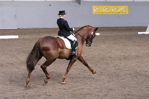
              DSN                       CASENet                     DDS-R

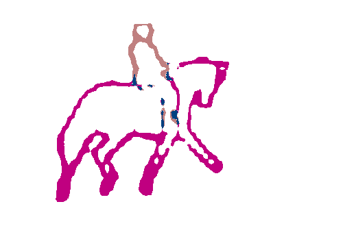
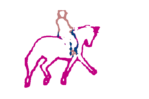
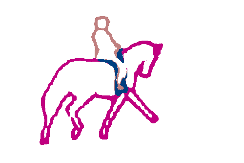
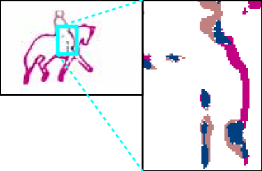
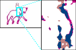
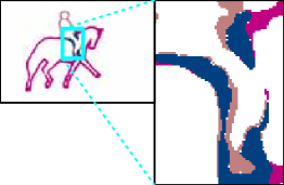
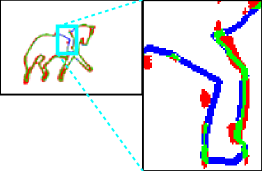
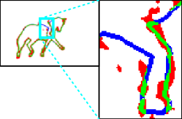
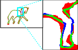
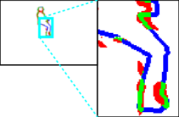
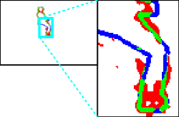
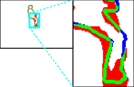
Figure 4: A qualitative comparison of DSN, CASENet and DDS-R. First row: the original image, ground truth, and category color codes. This image is taken from the SBD dataset Hariharan et al. (2011). Second row: the semantic edges predicted by different methods. Third row: an enlarged area of predicted edges. Fourth row: the predicted horse boundaries only. Last row: the predicted person boundaries only. Green, red, white, and blue pixels represent true positive, false positive, true negative, and false negative points, respectively, at the threshold of 0.5. Best viewed in color.

Table 5: ODS F-measure (%) of DDS-R/DDS-U and other competitors on the re-annotated SBD dataset Yu et al. (2018). The best performance of each column is highlighted in bold.

Methods	aer.	bike	bird	boat	bot.	bus	car	cat	cha.	cow	tab.	dog	hor.	mot.	per.	pot.	she.	sofa	train	tv	mean
With the “Thin” evaluation metric in Yu et al. (2018)
CASENet	74.5	59.7	73.4	48.0	67.1	78.6	67.3	76.2	47.5	69.7	36.2	75.7	72.7	61.3	74.8	42.6	71.8	48.9	71.7	54.9	63.6
SEAL	78.0	65.8	76.6	52.4	68.6	80.0	70.4	79.4	50.0	72.8	41.4	78.1	75.0	65.5	78.5	49.4	73.3	52.2	73.9	58.1	67.0
STEAL	77.1	63.6	76.2	51.1	68.0	80.4	70.0	76.8	49.4	71.9	40.4	78.1	74.7	64.5	75.7	45.4	73.5	47.5	73.5	58.7	65.8
Gated-SCNN	74.8	58.4	65.9	47.1	63.0	74.5	65.6	71.6	41.4	61.6	39.4	70.8	65.0	57.4	72.9	44.1	69.3	44.0	64.5	50.5	60.1
DDS-R	79.7	65.2	74.6	51.8	71.9	81.3	72.5	79.4	49.2	75.1	43.9	77.8	75.3	65.2	78.9	51.1	74.9	54.1	75.1	61.7	67.9
DDS-U	81.4	67.6	77.8	55.7	70.9	82.0	74.5	81.2	52.1	76.5	47.2	79.6	77.3	68.1	80.2	53.4	78.5	56.1	76.6	63.9	70.0
DFF	78.6	66.2	77.9	53.2	72.3	81.3	73.3	79.0	50.7	76.8	38.7	77.2	78.6	65.2	77.9	49.4	76.1	49.7	74.7	62.9	68.0
DDS-R	78.8	68.0	78.3	55.0	71.9	82.4	74.6	80.5	52.0	74.0	42.0	78.3	77.1	66.1	78.5	49.3	77.5	49.3	76.9	64.8	68.8
With the “Raw” evaluation metric in Yu et al. (2018)
CASENet	65.8	51.5	65.0	43.1	57.5	68.1	58.2	66.0	45.4	59.8	32.9	64.2	65.8	52.6	65.7	40.9	65.0	42.9	61.4	47.8	56.0
SEAL	75.3	60.5	75.1	51.2	65.4	76.1	67.9	75.9	49.7	69.5	39.9	74.8	72.7	62.1	74.2	48.4	72.3	49.3	70.6	56.7	64.4
STEAL	70.9	55.9	71.6	47.6	61.5	72.6	64.6	70.2	47.5	67.4	37.3	70.6	69.4	59.1	69.2	44.3	69.1	42.6	67.7	53.5	60.6
Gated-SCNN	66.8	50.1	59.4	44.2	54.9	64.6	57.9	62.2	39.6	50.9	35.9	59.5	56.5	48.9	64.2	41.3	64.0	35.6	54.2	45.5	52.8
DDS-R	75.6	61.1	71.0	49.5	67.7	76.1	67.2	74.2	48.8	69.1	40.4	72.5	71.7	60.4	73.4	49.6	70.6	49.5	71.9	59.4	64.0
DDS-U	78.4	62.7	75.6	53.4	67.8	78.5	71.4	77.4	51.3	72.8	44.5	74.7	74.8	64.3	76.3	51.9	77.3	51.9	73.7	62.9	67.1
DFF	72.3	58.4	73.4	48.7	65.4	74.8	66.4	72.5	47.8	70.1	34.7	69.2	71.5	58.7	70.2	47.5	71.2	43.7	69.5	59.1	62.3
DDS-R	74.2	61.2	71.3	51.9	65.5	77.3	68.0	73.8	50.0	66.0	39.4	70.8	70.5	58.9	71.8	49.0	72.6	44.7	71.6	62.2	63.5

5.3 Evaluation on SBD

In this part, we compare DDS-R/DDS-U on the SBD dataset Hariharan et al. (2011) with previous state-of-the-art methods, including InvDet Hariharan et al. (2011), HFL-FC8 Bertasius et al. (2015b), HFL-CRF Bertasius et al. (2015b), BNF Bertasius et al. (2016), WS Khoreva et al. (2016), DilConv Yu & Koltun (2016), DSN Yu et al. (2017), COB Maninis et al. (2017), CASENet Yu et al. (2017), SEAL Yu et al. (2018), STEAL Acuna et al. (2019), DFF Hu et al. (2019), and Gated-SCNN Takikawa et al. (2019). Among them, DFF Hu et al. (2019) shares the same distinct supervision problem as CASENet, so we also integrate DDS-R into DFF to demonstrate the generalizability of DDS-R. We adopt the same code implementation and training strategies for DFF-based DDS-R as the original DFF. Gated-SCNN Takikawa et al. (2019) learns semantic edges for improving the training of semantic segmentation. Hence, we retrain it for semantic edge detection by removing its segmentation loss and dual task loss, and the other settings are kept by default.

Results are summarized in Table 4. DDS-U achieves the state-of-the-art performance across all competitors. The ODS F-measure of the proposed DDS-U is 1.7% higher than SEAL and 3.4% higher than CASENet in terms of the metric in Hariharan et al. (2011), so delivering a new state-of-the-art. We can observe that DDS-R can also improve the performance of DFF Hu et al. (2019). Therefore, the proposed DDS can be viewed as a general idea to improve SED. The improvement from CASENet to DDS is also larger than the improvement of STEAL. Moreover, InvDet Hariharan et al. (2011) is a non-deep learning based approach which shows competitive results among other conventional approaches. COB Maninis et al. (2017) is a state-of-the-art category-agnostic edge detection method, and combining it with semantic segmentation of DilConv Yu & Koltun (2016) produces a competitive semantic edge detector. COB’s superiority over DilConv reflects the effectiveness of its fusion algorithm. The fact that both CASENet and DDS-R/DDS-U outperform COB illustrates the importance of directly learning semantic edges, because the combination of binary edges and semantic segmentation is insufficient for SED. The average runtime of DSN, CASENet, and DDS is shown in Table 6. DDS can generate state-of-the-art semantic edges with only a slight reduction in speed.

Table 6: Average runtime per image on the SBD dataset Hariharan et al. (2011).

Methods	DSN	CASENet	SEAL	DDS
Time (s)	0.171	0.166	0.166	0.175

Table 7: ODS F-measure (%) of DDS-R/DDS-U and other competitors on the Cityscapes dataset Cordts et al. (2016). The best performance of each column is highlighted in bold.

Methods	road	sid.	bui.	wall	fen.	pole	light	sign	veg.	ter.	sky	per.	rider	car	tru.	bus	tra.	mot.	bike	mean
With the “Thin” evaluation metric in Yu et al. (2018)
CASENet	86.2	74.9	74.5	47.6	46.5	72.8	70.0	73.3	79.3	57.0	86.5	80.4	66.8	88.3	49.3	64.6	47.8	55.8	71.9	68.1
SEAL	87.6	77.5	75.9	47.6	46.3	75.5	71.2	75.4	80.9	60.1	87.4	81.5	68.9	88.9	50.2	67.8	44.1	52.7	73.0	69.1
STEAL	87.8	77.2	76.4	49.5	49.2	74.9	73.2	76.3	80.8	58.9	86.8	80.2	69.0	83.2	52.1	67.7	53.2	55.8	72.8	69.7
Gated-SCNN	88.9	78.7	78.3	51.3	52.3	78.6	78.7	78.0	82.2	62.3	87.7	83.5	70.8	90.6	33.1	60.4	31.6	50.9	74.4	69.1
DDS-R	86.1	76.5	76.1	49.8	49.9	74.6	76.4	76.8	80.4	58.9	87.2	83.5	70.7	89.6	52.9	71.5	50.4	61.8	74.4	70.9
DDS-U	89.2	79.2	79.0	51.9	52.9	77.5	79.4	80.3	82.6	61.4	88.8	85.0	74.1	91.1	59.0	76.0	55.7	63.6	76.3	73.8
DFF	89.4	80.1	79.6	51.3	54.5	81.3	81.3	81.2	83.6	62.9	89.0	85.4	75.8	91.6	54.9	73.9	51.9	64.3	76.4	74.1
DDS-R	89.7	79.4	80.4	52.1	53.0	82.4	81.9	80.9	83.9	62.0	89.4	86.0	77.8	92.3	59.8	74.8	55.3	64.4	77.4	74.9
With the “Raw” evaluation metric in Yu et al. (2018)
CASENet	66.8	64.6	66.8	39.4	40.6	71.7	64.2	65.1	71.1	50.2	80.3	73.1	58.6	77.0	42.0	53.2	39.1	46.1	62.2	59.6
SEAL	84.4	73.5	72.7	43.4	43.2	76.1	68.5	69.8	77.2	57.5	85.3	77.6	63.6	84.9	48.6	61.9	41.2	49.0	66.7	65.5
STEAL	75.8	68.5	69.8	34.9	36.1	73.4	66.7	67.7	73.5	49.7	78.7	72.9	59.1	76.5	35.3	52.8	37.7	43.8	63.7	59.8
Gated-SCNN	77.3	69.7	74.8	38.2	40.1	79.7	72.6	72.4	77.7	54.2	82.0	77.7	62.0	86.1	17.1	37.7	14.3	37.5	66.8	59.9
DDS-R	73.3	65.9	70.9	33.2	37.4	76.8	70.1	70.2	74.6	50.4	80.6	77.9	62.6	82.5	37.1	55.0	32.0	49.4	66.1	61.4
DDS-U	83.5	74.2	76.0	37.5	40.7	79.5	75.6	75.3	79.3	55.7	85.3	81.1	67.1	87.9	44.6	63.4	40.4	52.3	70.0	66.8
DFF	72.8	68.3	72.6	37.2	42.2	79.6	75.0	73.9	75.3	51.4	80.8	78.6	69.4	83.0	44.1	56.7	38.4	52.0	68.8	64.2
DDS-R	80.8	70.8	76.4	38.9	41.1	80.0	78.2	76.3	79.2	53.2	82.5	81.8	72.2	86.2	44.8	59.5	37.6	55.7	71.3	66.7

     DSN-Horse        DSN-Person         CASENet             DDS-R

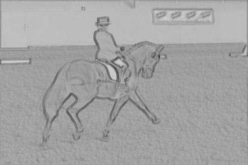
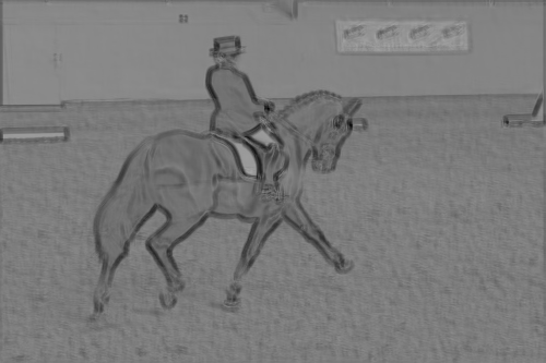
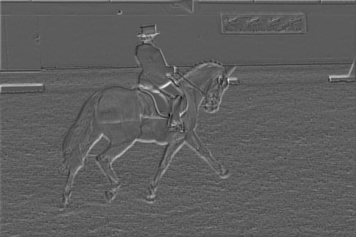
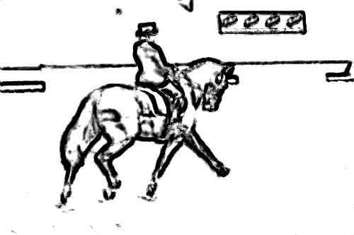
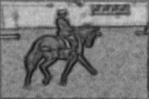
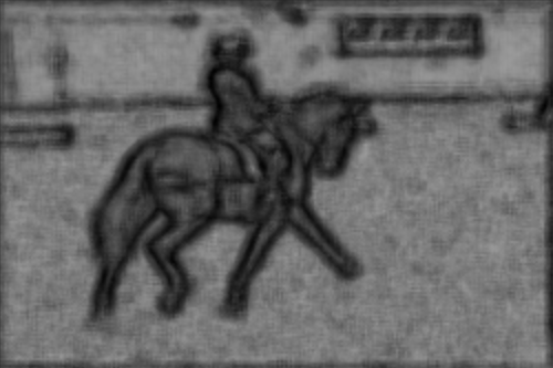
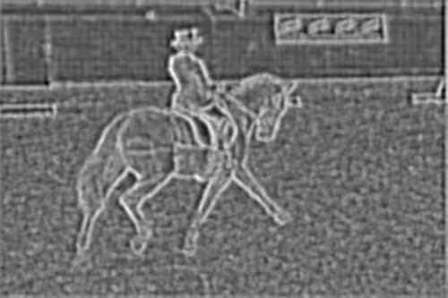
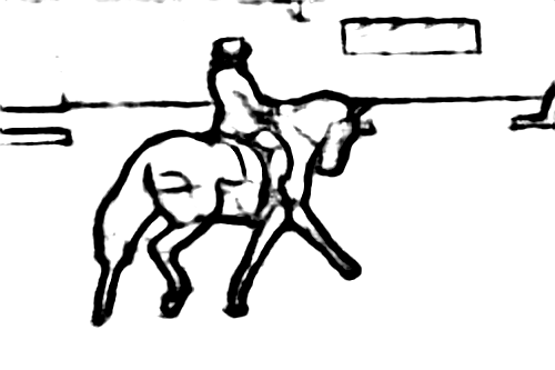
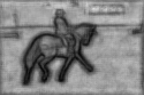
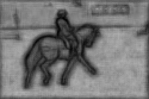
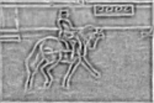
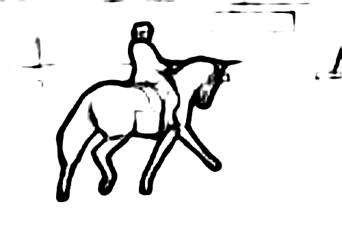
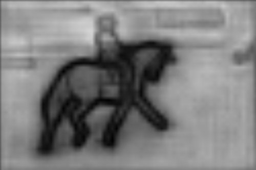
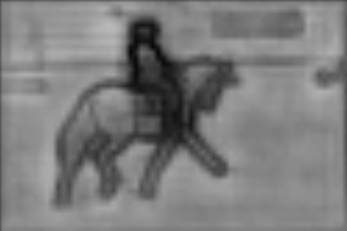
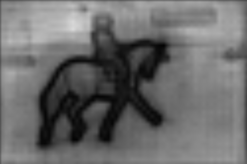
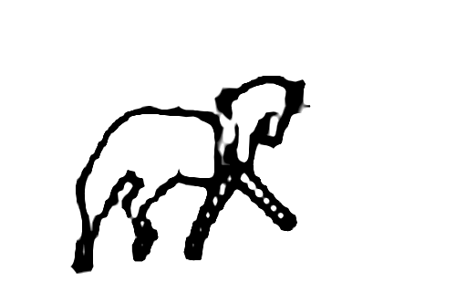
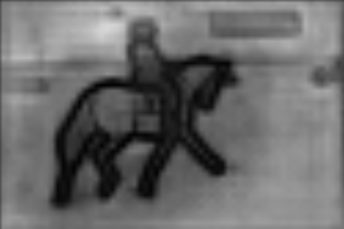
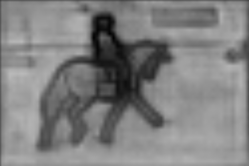
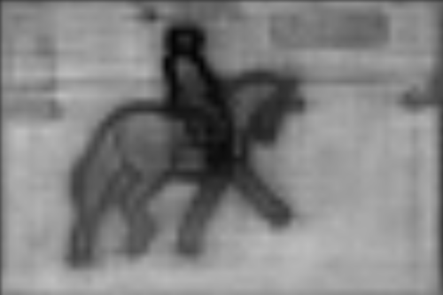
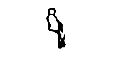
[2pt] Side-1
[2pt] Side-2
[2pt] Side-3
[2pt] Side-4 [2pt] Side5-Horse
[2pt] Side-5 [2pt] Side5-Person

Figure 5: Side activation maps on the input image of Fig. 4. The first two columns display DSN’s side class classification activation for the classes of horse and person, respectively. The last two columns show the side features of Side-1 $\sim$ Side-3 and class classification activation of Side-5 for CASENet and our DDS-R, respectively. These images are obtained by normalizing the activation to $[0,255]$. Note that all activations are directly outputted without any non-linearization, e.g., sigmoid function.

aeroplane	bicycle	bird	boat	bottle	bus	car	cat	chair	cow
dining table	dog	horse	motorbike	person	potted plant	sheep	sofa	train	tv monitor

Original Images

Ground Truth
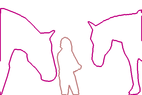
DSN
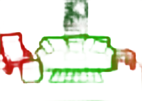
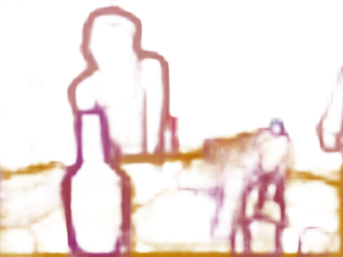
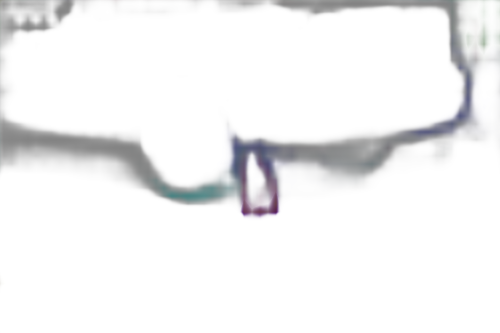
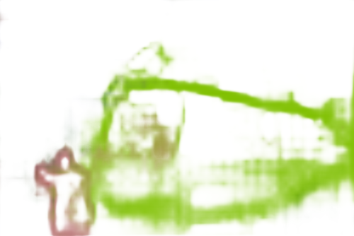
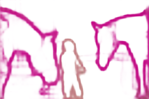
CASENet
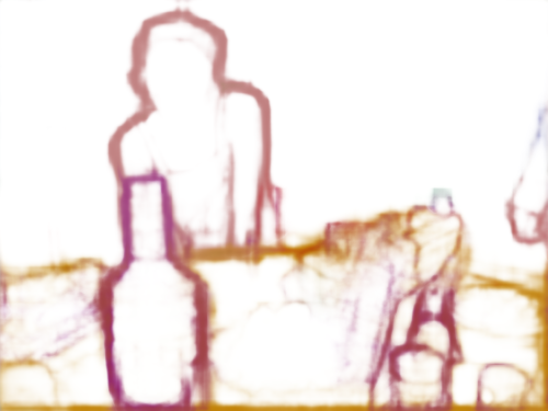
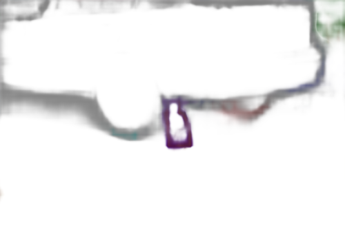
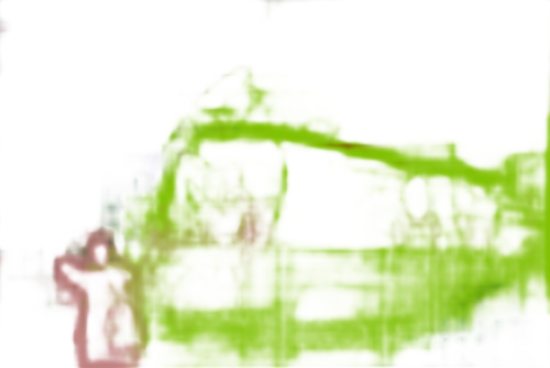
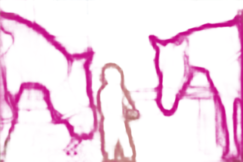
SEAL
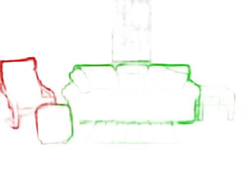
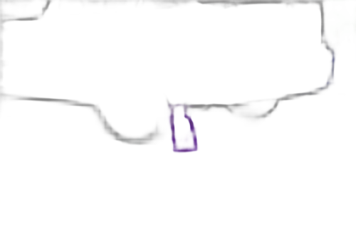
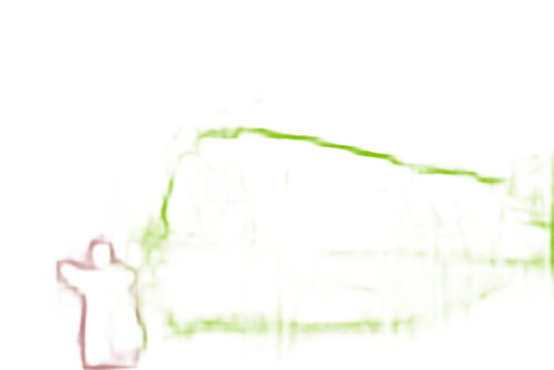
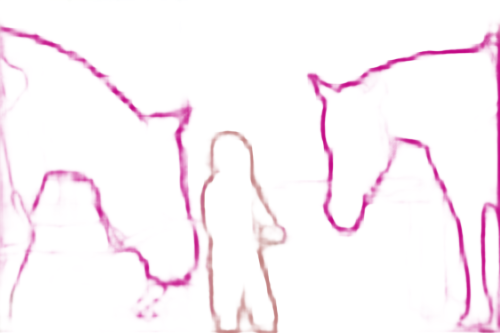
STEAL
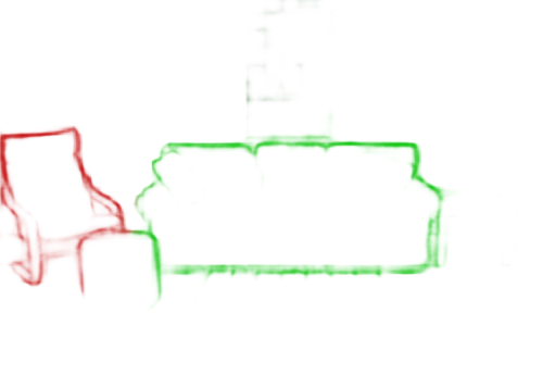
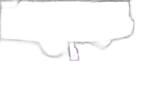
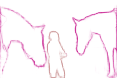
DFF
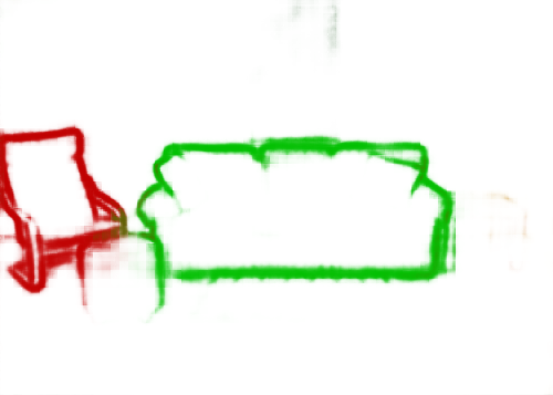
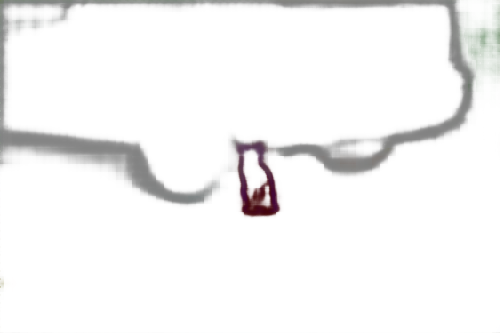
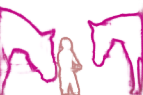
DDS-R
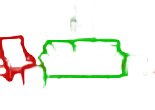
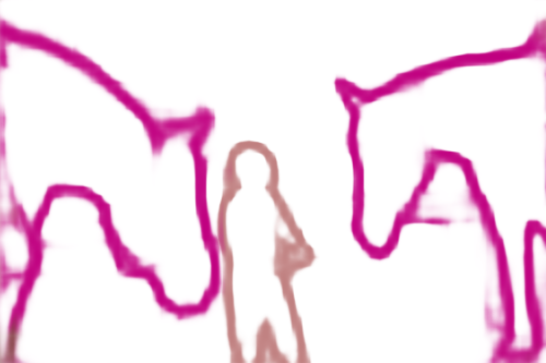
DDS-U

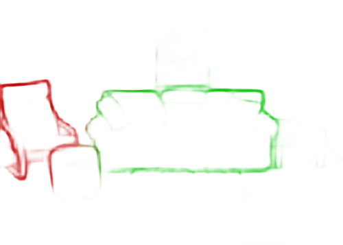
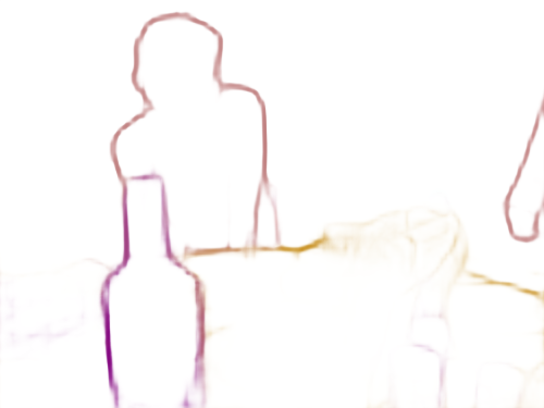
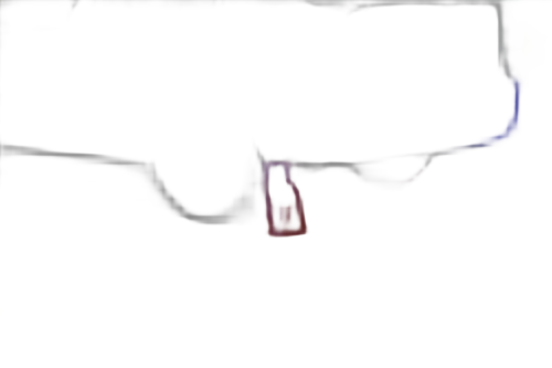
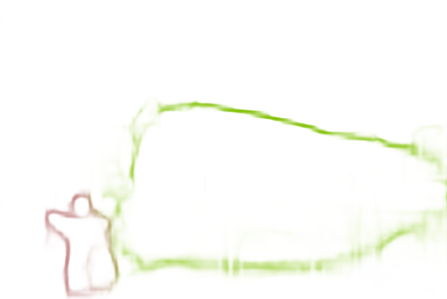
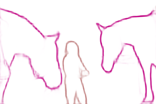
Figure 6: Some examples from SBD dataset Hariharan et al. (2011). From top to bottom: color codes, original images, ground truth, DSN, CASENet Yu et al. (2017), SEAL Yu et al. (2018), STEAL Acuna et al. (2019), DFF Hu et al. (2019), our DDS-R and DDS-U. We follow the color coding protocol in Yu et al. (2018).

road	sidewalk	building	wall	fence	pole	traffic light	traffic sign	vegetation	terrain
sky	person	rider	car	truck	bus	train	motorcycle	bicycle

Original Images

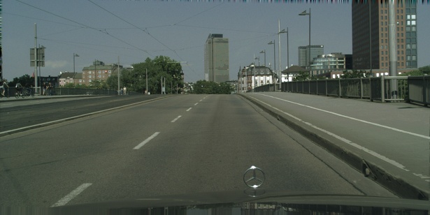
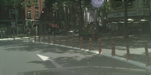
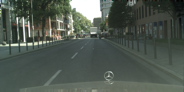
Ground Truth
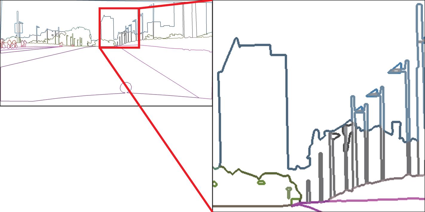
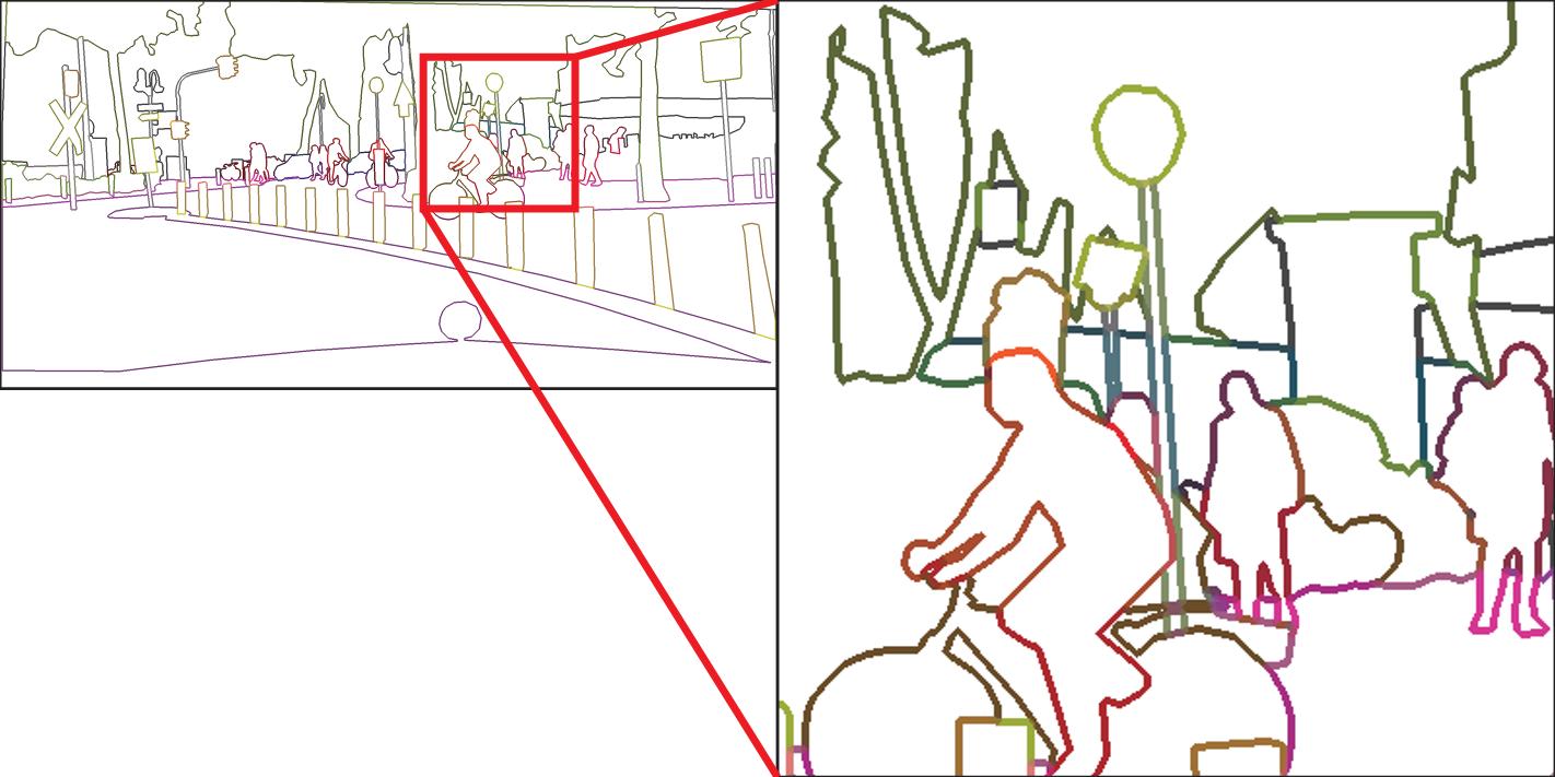
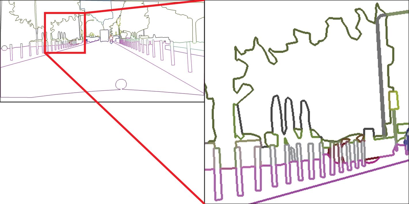
CASENet
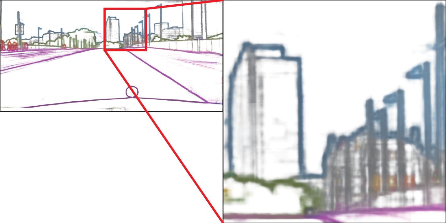
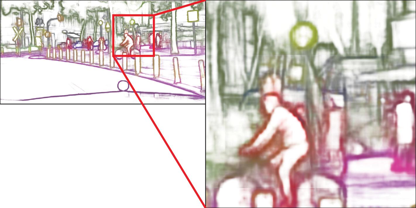
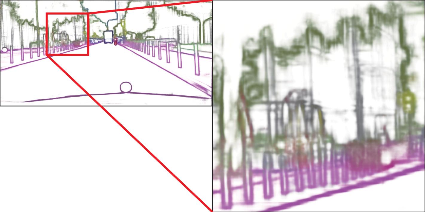
SEAL
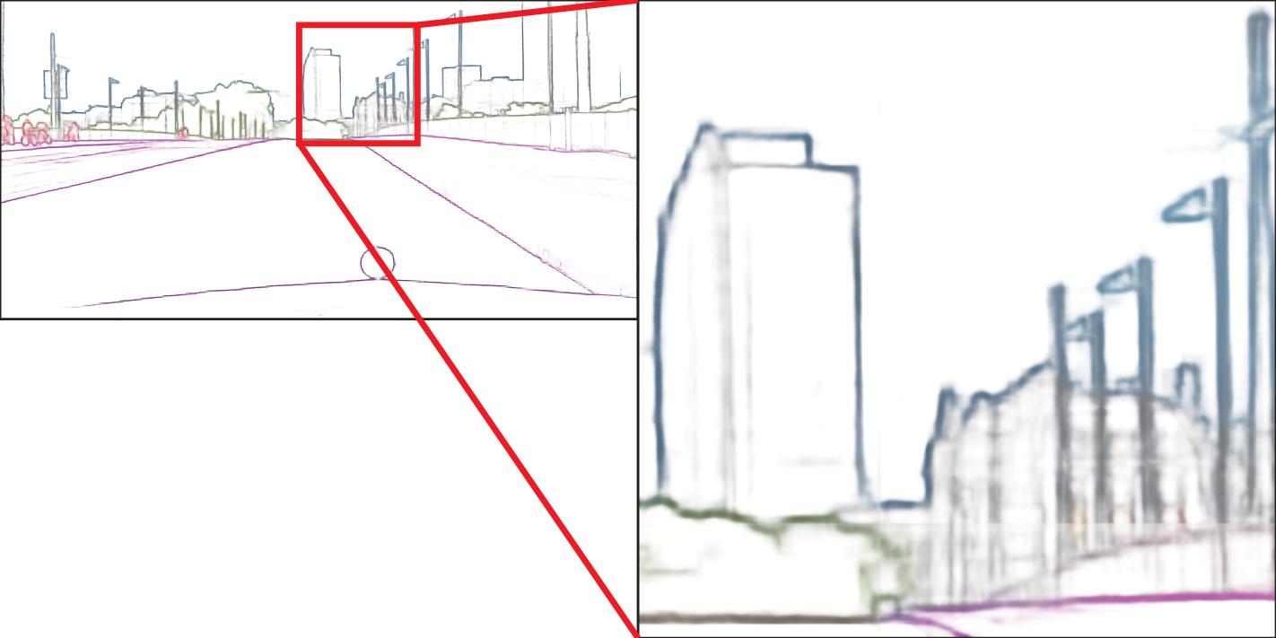
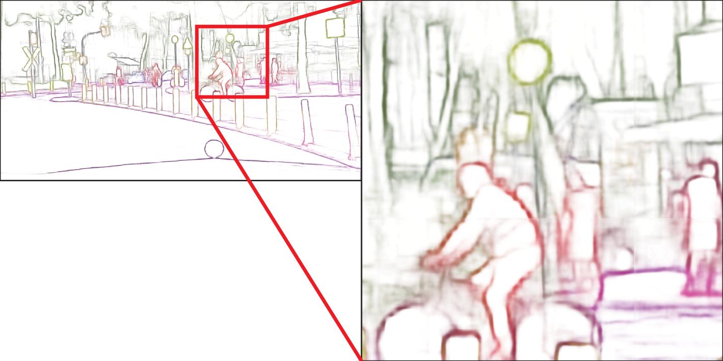
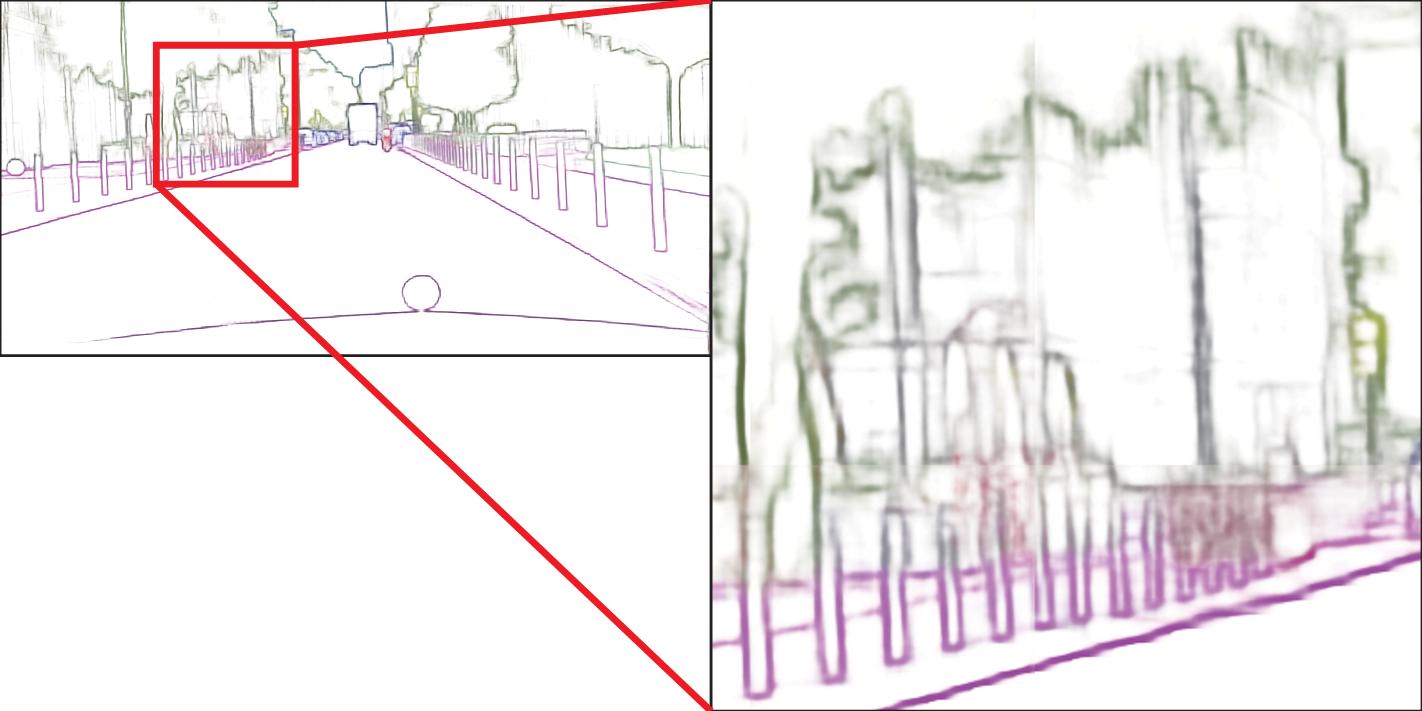
STEAL
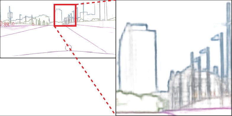
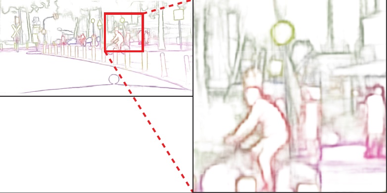
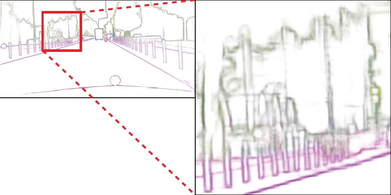
DFF
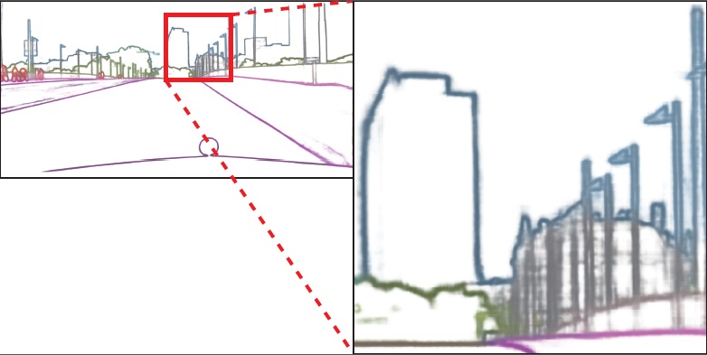
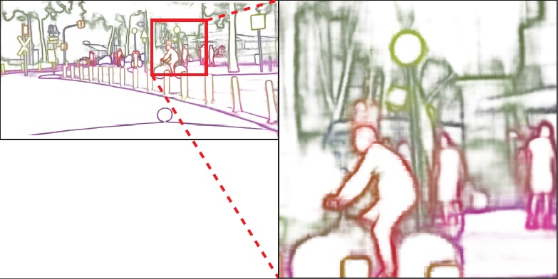
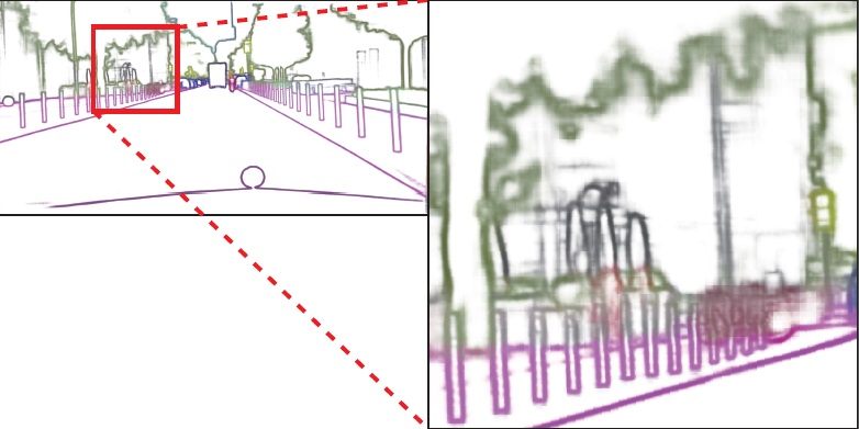
DDS-R
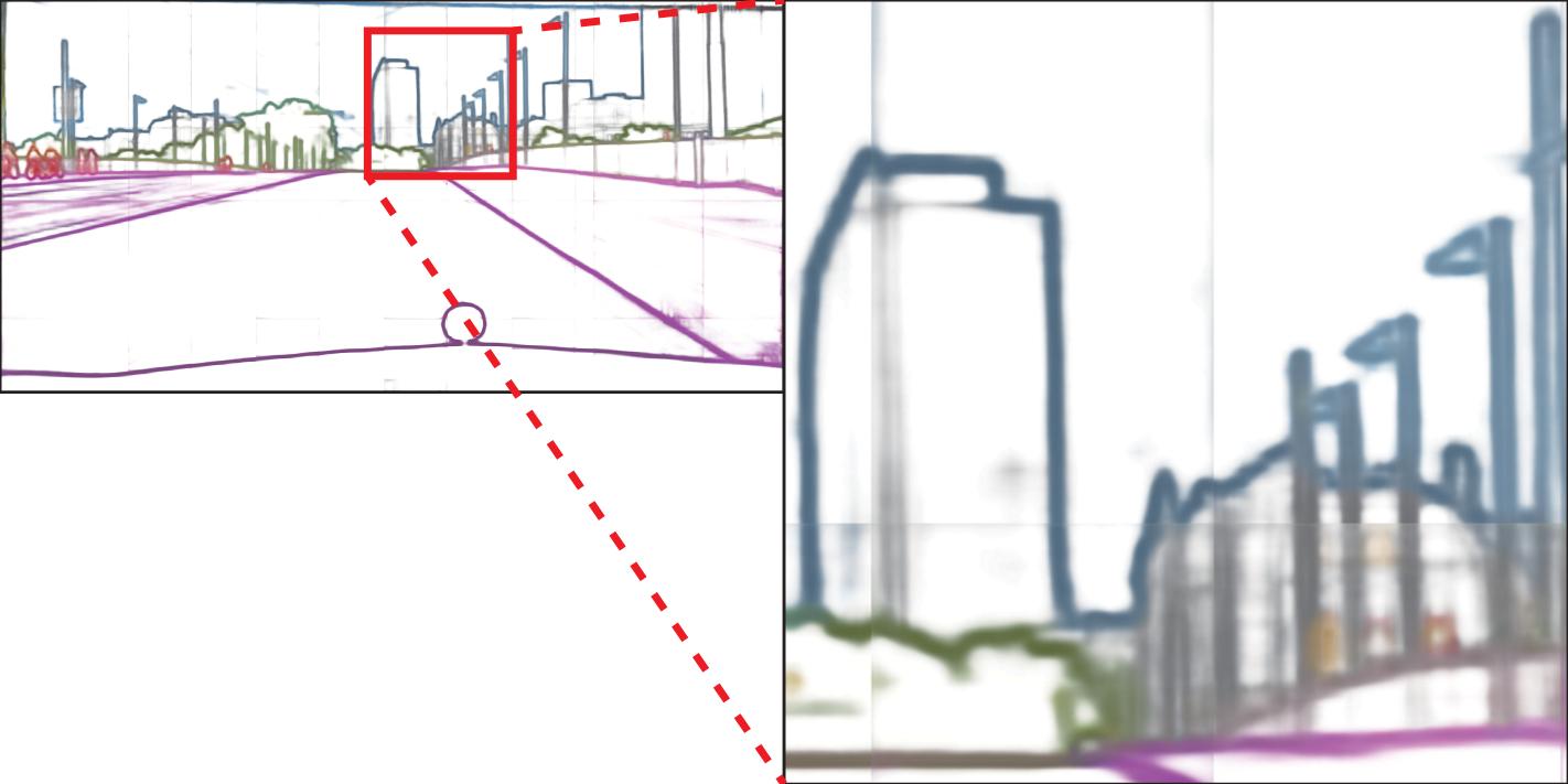
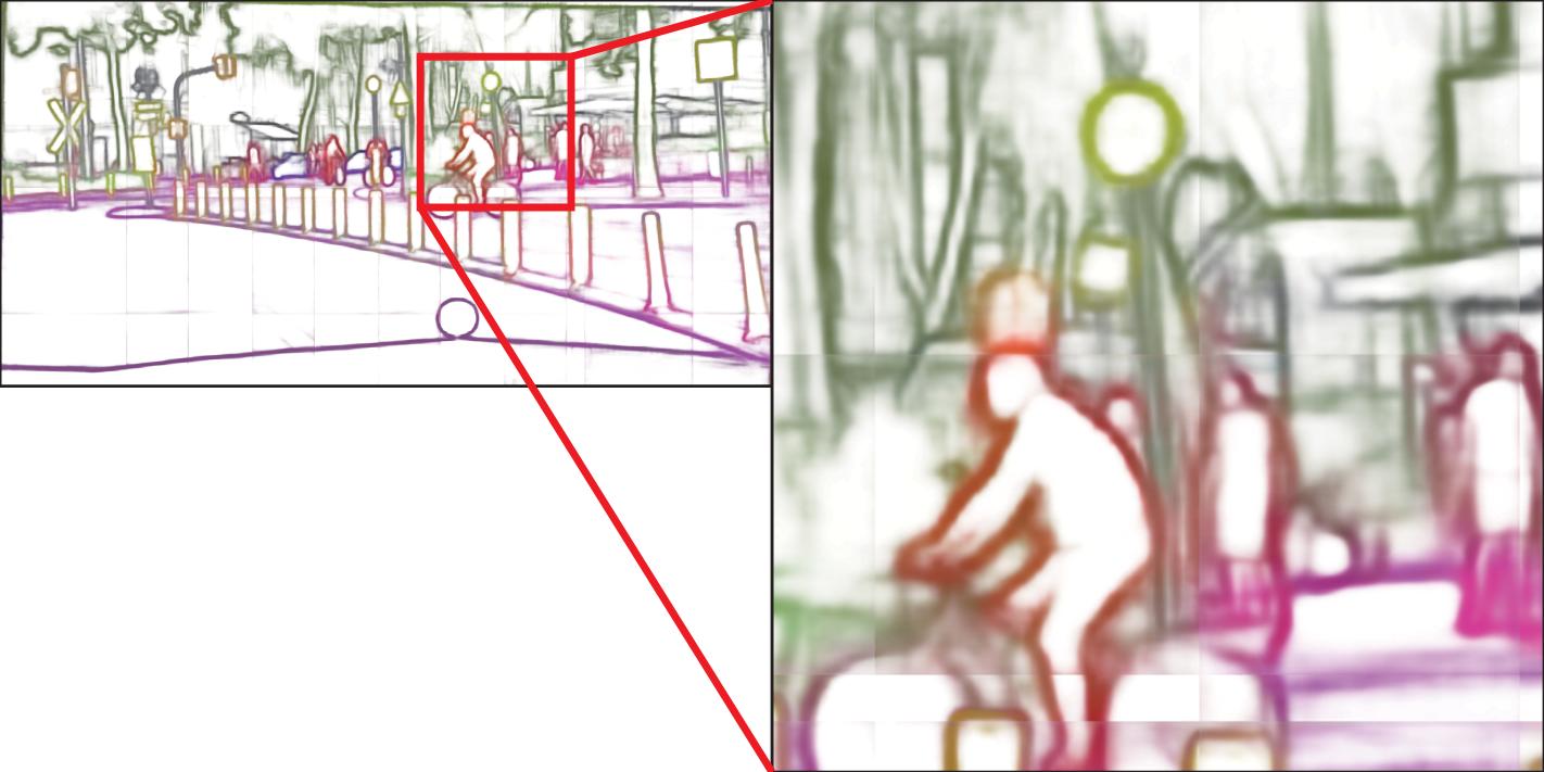
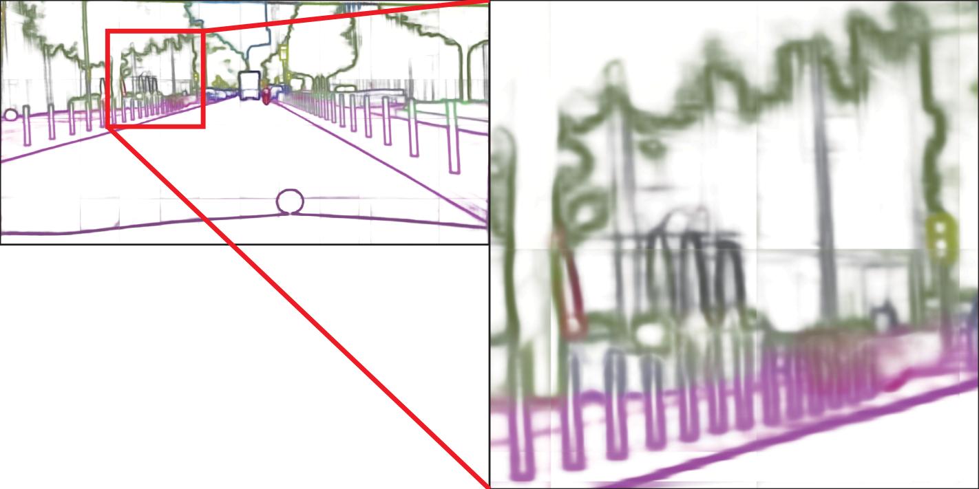
DDS-U

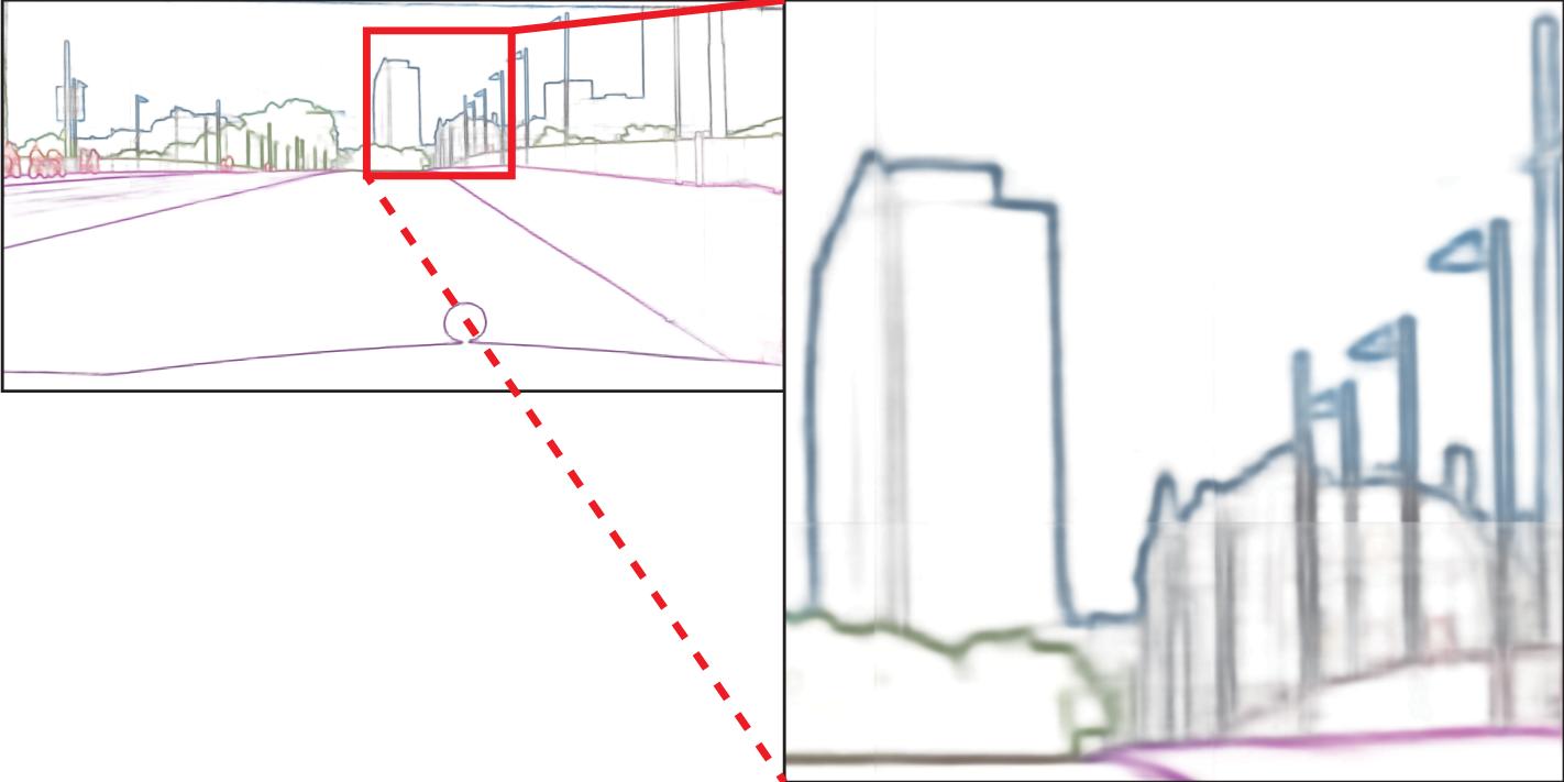
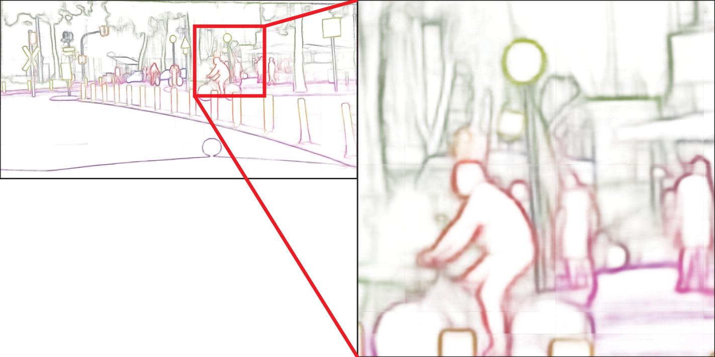
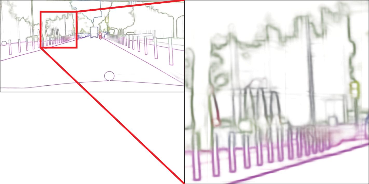
Figure 7: Some examples from Cityscapes dataset Cordts et al. (2016). From top to bottom: color codes, original images, ground truth, CASENet Yu et al. (2017), SEAL Yu et al. (2018), STEAL Acuna et al. (2019), DFF Hu et al. (2019), our DDS-R and DDS-U. We follow the color coding protocol in Yu et al. (2018). The produced edges of DDS are smoother and clearer.

Yu et al. Yu et al. (2018) discovered that some of the original SBD labels are a little noisy, so they re-annotated 1059 images from the test set to form a new test set. We compare our method with CASENet Yu et al. (2017), SEAL Yu et al. (2018), STEAL Acuna et al. (2019), Gated-SCNN Takikawa et al. (2019), and DFF Hu et al. (2019) on this new dataset. The results are shown in Table 5. DDS can improve the performance for both CASENet and DFF in terms of all evaluation metrics. Specifically, the ODS F-measures of DDS-U is 3.0% and 2.7% higher than recent SEAL Yu et al. (2018) in terms of the “Thin” and “Raw” metrics in Yu et al. (2018), respectively. Note that SEAL retrains CASENet with a new training strategy: i.e., simultaneous alignment and learning. With the same training strategy, DDS-R obtains a 4.3% and 8.0% higher ODS F-measure than CASENet in terms of the “Thin” and “Raw” metrics in Yu et al. (2018), respectively.

To better visualize the edge prediction results, an example is shown in Fig. 4. We also show the normalized images of side activation in Fig. 5. All activations are obtained before sigmoid non-linearization. For a simple arrangement of figures, we do not display Side-4 activation of DDS-R. From Side-1 to Side-3, one can see that the feature maps of DDS-R are significantly clearer than those of DSN and CASENet. Clear category-agnostic edges can be found with DDS-R, while DSN and CASENet suffer from noisy activation. For example, in CASENet, without imposing deep supervision on Side-1 $\sim$ Side-3, edge activation can barely be found. For category classification activation, DDS-R can separate horse and person clearly, while DSN and CASENet can not. Therefore, the information converters also help to better optimize Side-5 for category-specific classification. This further verifies the feasibility of the proposed DDS architecture.

More qualitative examples are displayed in Fig. 6. DDS-R/DDS-U can produce clearer and smother edges than other detectors. In the second column, it is interesting to note that most detectors can recognize the boundaries of the objects with missing annotations, i.e., the obscured dining table and human arm. In the third column, DDS-R/DDS-U can generate strong responses at the boundaries of the small cat, while all other detectors only have weak or noisy responses. This demonstrates that DDS is more robust for detecting small objects. We also find that DDS-U and SEAL can generate thinner edges, suggesting that training with regular unweighted sigmoid cross entropy loss and refined ground-truth edges is helpful for accurately locating thin boundaries.

5.4 Evaluation on Cityscapes

The Cityscapes dataset Cordts et al. (2016) is more challenging than SBD Hariharan et al. (2011). The images in Cityscapes are captured in more complicated scenes, usually in urban street scenes in different cities. There are more objects, especially overlapping objects, in each image. Hence, we also adopt Cityscapes for evaluating semantic edge detectors using the “Thin” and “Raw” metrics in Yu et al. (2018). We compare DDS with CASENet Yu et al. (2017), SEAL Yu et al. (2018), STEAL Acuna et al. (2019), DFF Hu et al. (2019), and Gated-SCNN Takikawa et al. (2019).

The evaluation results are reported in Table 7. Both DDS-R and DDS-U significantly outperform other methods in terms of both “Thin” and “Raw” metrics. With the same loss function, the ODS F-measure of DDS-R is 2.8% higher than CASENet in terms of the “Thin” metric in Yu et al. (2018), and DDS-U is 4.7% higher than SEAL correspondingly. STEAL and Gated-SCNN achieve similar performance, and both are much worse than DDS-R and DDS-U. Note that Gated-SCNN is the state-of-the-art semantic segmentation model, suggesting that it is necessary to study semantic edge detection rather than directly applying existing related techniques. Some qualitative comparisons are shown in Fig. 7. We can see that DDS-R/DDS-U produces smoother and clearer edges in various complicated scenarios, which is brought by the low-level binary edge supervision of DDS.

6 Conclusion

In this paper, we study the SED problem. Previous methods suggest that deep supervision is not necessary Yu et al. (2017, 2018); Hu et al. (2019) for SED. Here, we show that this is false and, with proper architecture re-design, that the network can be deeply supervised to improve detection results. The core of our approach is the introduction of the novel information converter, which plays a central role in resolving the distinct supervision targets by successfully applying category-aware edges at the top side and the category-agnostic edges at bottom sides. The proposed DDS achieves state-of-the-art performance on the popular SBD Hariharan et al. (2011) and Cityscapes Cordts et al. (2016) datasets. Our idea to leverage deep supervision for training a deep network opens up a new path towards putting more emphasis utilizing rich feature hierarchies from deep networks for SED as well as other high-level tasks such as semantic segmentation Maninis et al. (2017); Chen et al. (2016), object detection Ferrari et al. (2008); Maninis et al. (2017), and instance segmentation Kirillov et al. (2017); Hayder et al. (2017).

Future Work. Besides category-agnostic edge detection and SED, relevant tasks commonly exist in computer vision Zamir et al. (2018), such as segmentation and saliency detection, object detection and keypoint detection, edge detection and skeleton extraction. Building multi-task networks to solve relevant tasks is a good way to save computational resources in practical applications Hou et al. (2018). However, distinct supervision targets usually prevent this goal, as shown in this paper. From this point of view, the proposed DDS provides a new perspective to multi-task learning. In the future, we plan to leverage the idea of information converter for more relevant tasks.

References

- Acuna et al. (2019) Acuna, D., Kar, A., & Fidler, S. (2019). Devil is in the edges: Learning semantic boundaries from noisy annotations. In IEEE Conf. Comput. Vis. Pattern Recog. (pp. 11075–11083).
- Amer et al. (2015) Amer, M. R., Yousefi, S., Raich, R., & Todorovic, S. (2015). Monocular extraction of 2.1 d sketch using constrained convex optimization. Int. J. Comput. Vis., 112(1), pp. 23–42.
- Arbeláez et al. (2011) Arbeláez, P., Maire, M., Fowlkes, C., & Malik, J. (2011). Contour detection and hierarchical image segmentation. IEEE Trans. Pattern Anal. Mach. Intell., 33(5), pp. 898–916.
- Bertasius et al. (2015a) Bertasius, G., Shi, J., & Torresani, L. (2015a). DeepEdge: A multi-scale bifurcated deep network for top-down contour detection. In IEEE Conf. Comput. Vis. Pattern Recog. (pp. 4380–4389).
- Bertasius et al. (2015b) Bertasius, G., Shi, J., & Torresani, L. (2015b). High-for-low and low-for-high: Efficient boundary detection from deep object features and its applications to high-level vision. In Int. Conf. Comput. Vis. (pp. 504–512).
- Bertasius et al. (2016) Bertasius, G., Shi, J., & Torresani, L. (2016). Semantic segmentation with boundary neural fields. In IEEE Conf. Comput. Vis. Pattern Recog. (pp. 3602–3610).
- Bian et al. (2021) Bian, J.-W., Zhan, H., Wang, N., Li, Z., Zhang, L., Shen, C., et al. (2021). Unsupervised scale-consistent depth learning from video. Int. J. Comput. Vis., 129, pp. 2548–2564.
- Canny (1986) Canny, J. (1986). A computational approach to edge detection. IEEE Trans. Pattern Anal. Mach. Intell., 8(6), pp. 679–698.
- Chan et al. (2015) Chan, T.-H., Jia, K., Gao, S., Lu, J., Zeng, Z., & Ma, Y. (2015). PCANet: A simple deep learning baseline for image classification? IEEE Trans. Image Process., 24(12), pp. 5017–5032.
- Chen et al. (2016) Chen, L.-C., Barron, J. T., Papandreou, G., Murphy, K., & Yuille, A. L. (2016). Semantic image segmentation with task-specific edge detection using CNNs and a discriminatively trained domain transform. In IEEE Conf. Comput. Vis. Pattern Recog. (pp. 4545–4554).
- Cordts et al. (2016) Cordts, M., Omran, M., Ramos, S., Rehfeld, T., Enzweiler, M., Benenson, R., et al. (2016). The cityscapes dataset for semantic urban scene understanding. In IEEE Conf. Comput. Vis. Pattern Recog. (pp. 3213–3223).
- Deng et al. (2018) Deng, R., Shen, C., Liu, S., Wang, H., & Liu, X. (2018). Learning to predict crisp boundaries. In Eur. Conf. Comput. Vis. (pp. 570–586).
- Dollár & Zitnick (2015) Dollár, P., & Zitnick, C. L. (2015). Fast edge detection using structured forests. IEEE Trans. Pattern Anal. Mach. Intell., 37(8), pp. 1558–1570.
- Ferrari et al. (2008) Ferrari, V., Fevrier, L., Jurie, F., & Schmid, C. (2008). Groups of adjacent contour segments for object detection. IEEE Trans. Pattern Anal. Mach. Intell., 30(1), pp. 36–51.
- Ferrari et al. (2010) Ferrari, V., Jurie, F., & Schmid, C. (2010). From images to shape models for object detection. Int. J. Comput. Vis., 87(3), pp. 284–303.
- Ganin & Lempitsky (2014) Ganin, Y., & Lempitsky, V. (2014). N4-Fields: Neural network nearest neighbor fields for image transforms. In Asian Conf. Comput. Vis. (pp. 536–551).
- Hardie & Boncelet (1995) Hardie, R. C., & Boncelet, C. G. (1995). Gradient-based edge detection using nonlinear edge enhancing prefilters. IEEE Trans. Image Process., 4(11), pp. 1572–1577.
- Hariharan et al. (2011) Hariharan, B., Arbeláez, P., Bourdev, L., Maji, S., & Malik, J. (2011). Semantic contours from inverse detectors. In Int. Conf. Comput. Vis. (pp. 991–998).
- Hayder et al. (2017) Hayder, Z., He, X., & Salzmann, M. (2017). Boundary-aware instance segmentation. In IEEE Conf. Comput. Vis. Pattern Recog. (pp. 5696–5704).
- He et al. (2016) He, K., Zhang, X., Ren, S., & Sun, J. (2016). Deep residual learning for image recognition. In IEEE Conf. Comput. Vis. Pattern Recog. (pp. 770–778).
- Henstock & Chelberg (1996) Henstock, P. V., & Chelberg, D. M. (1996). Automatic gradient threshold determination for edge detection. IEEE Trans. Image Process., 5(5), pp. 784–787.
- Hinton et al. (2006) Hinton, G. E., Osindero, S., & Teh, Y.-W. (2006). A fast learning algorithm for deep belief nets. Neural Computation, 18(7), pp. 1527–1554.
- Hou et al. (2019) Hou, Q., Cheng, M.-M., Hu, X., Borji, A., Tu, Z., & Torr, P. (2019). Deeply supervised salient object detection with short connections. IEEE Trans. Pattern Anal. Mach. Intell., 41(4), pp. 815–828.
- Hou et al. (2018) Hou, Q., Liu, J., Cheng, M.-M., Borji, A., & Torr, P. H. (2018). Three birds one stone: A unified framework for salient object segmentation, edge detection and skeleton extraction. arXiv preprint arXiv:1803.09860.
- Hu et al. (2018) Hu, X., Liu, Y., Wang, K., & Ren, B. (2018). Learning hybrid convolutional features for edge detection. Neurocomputing.
- Hu et al. (2019) Hu, Y., Chen, Y., Li, X., & Feng, J. (2019). Dynamic feature fusion for semantic edge detection. In Int. Joint Conf. Artif. Intell. (pp. 782–788).
- Ioffe & Szegedy (2015) Ioffe, S., & Szegedy, C. (2015). Batch normalization: Accelerating deep network training by reducing internal covariate shift. In Int. Conf. Mach. Learn. (pp. 448–456).
- Jia et al. (2014) Jia, Y., Shelhamer, E., Donahue, J., Karayev, S., Long, J., Girshick, R., et al. (2014). Caffe: Convolutional architecture for fast feature embedding. In ACM Int. Conf. Multimedia. (pp. 675–678).
- Khoreva et al. (2016) Khoreva, A., Benenson, R., Omran, M., Hein, M., & Schiele, B. (2016). Weakly supervised object boundaries. In IEEE Conf. Comput. Vis. Pattern Recog. (pp. 183–192).
- Kirillov et al. (2017) Kirillov, A., Levinkov, E., Andres, B., Savchynskyy, B., & Rother, C. (2017). Instancecut: from edges to instances with multicut. In IEEE Conf. Comput. Vis. Pattern Recog. (pp. 5008–5017).
- Kokkinos (2016) Kokkinos, I. (2016). Pushing the boundaries of boundary detection using deep learning. In Int. Conf. Learn. Represent. (pp. 1–12).
- Konishi et al. (2003) Konishi, S., Yuille, A. L., Coughlan, J. M., & Zhu, S. C. (2003). Statistical edge detection: Learning and evaluating edge cues. IEEE Trans. Pattern Anal. Mach. Intell., 25(1), pp. 57–74.
- Lee et al. (2015) Lee, C.-Y., Xie, S., Gallagher, P., Zhang, Z., & Tu, Z. (2015). Deeply-supervised nets. In Artificial Intelligence and Statistics. (pp. 562–570).
- Lim et al. (2013) Lim, J. J., Zitnick, C. L., & Dollár, P. (2013). Sketch tokens: A learned mid-level representation for contour and object detection. In IEEE Conf. Comput. Vis. Pattern Recog. (pp. 3158–3165).
- Lin et al. (2017) Lin, T.-Y., Dollár, P., Girshick, R., He, K., Hariharan, B., & Belongie, S. (2017). Feature pyramid networks for object detection. In IEEE Conf. Comput. Vis. Pattern Recog. (pp. 2117–2125).
- Lin et al. (2020) Lin, T.-Y., Goyal, P., Girshick, R., He, K., & Dollár, P. (2020). Focal loss for dense object detection. IEEE Trans. Pattern Anal. Mach. Intell., 42(2), pp. 318–327.
- Lin et al. (2014) Lin, T.-Y., Maire, M., Belongie, S., Hays, J., Perona, P., Ramanan, D., et al. (2014). Microsoft COCO: Common objects in context. In Eur. Conf. Comput. Vis. (pp. 740–755).
- Liu et al. (2016) Liu, W., Anguelov, D., Erhan, D., Szegedy, C., Reed, S., Fu, C.-Y., et al. (2016). SSD: Single shot multibox detector. In Eur. Conf. Comput. Vis. (pp. 21–37).
- Liu et al. (2019) Liu, Y., Cheng, M.-M., Hu, X., Bian, J.-W., Zhang, L., Bai, X., et al. (2019). Richer convolutional features for edge detection. IEEE Trans. Pattern Anal. Mach. Intell., 41(8), pp. 1939–1946.
- Liu et al. (2017) Liu, Y., Cheng, M.-M., Hu, X., Wang, K., & Bai, X. (2017). Richer convolutional features for edge detection. In IEEE Conf. Comput. Vis. Pattern Recog. (pp. 3000–3009).
- Liu et al. (2018) Liu, Y., Jiang, P.-T., Petrosyan, V., Li, S.-J., Bian, J., Zhang, L., et al. (2018). DEL: deep embedding learning for efficient image segmentation. In Int. Joint Conf. Artif. Intell. (pp. 864–870).
- Mafi et al. (2018) Mafi, M., Rajaei, H., Cabrerizo, M., & Adjouadi, M. (2018). A robust edge detection approach in the presence of high impulse noise intensity through switching adaptive median and fixed weighted mean filtering. IEEE Trans. Image Process., 27(11), pp. 5475–5490.
- Maninis et al. (2017) Maninis, K.-K., Pont-Tuset, J., Arbelaez, P., & Van Gool, L. (2017). Convolutional oriented boundaries: From image segmentation to high-level tasks. IEEE Trans. Pattern Anal. Mach. Intell., 40(4), pp. 819–833.
- Martin et al. (2004) Martin, D. R., Fowlkes, C. C., & Malik, J. (2004). Learning to detect natural image boundaries using local brightness, color, and texture cues. IEEE Trans. Pattern Anal. Mach. Intell., 26(5), pp. 530–549.
- Nair & Hinton (2010) Nair, V., & Hinton, G. E. (2010). Rectified linear units improve restricted Boltzmann machines. In Int. Conf. Mach. Learn. (pp. 807–814).
- Ramalingam et al. (2010) Ramalingam, S., Bouaziz, S., Sturm, P., & Brand, M. (2010). Skyline2gps: Localization in urban canyons using omni-skylines. In IEEERSJ Int. Conf. Intell. Robot. Syst. (pp. 3816–3823).
- Shan et al. (2014) Shan, Q., Curless, B., Furukawa, Y., Hernandez, C., & Seitz, S. M. (2014). Occluding contours for multi-view stereo. In IEEE Conf. Comput. Vis. Pattern Recog. (pp. 4002–4009).
- Shen et al. (2015) Shen, W., Wang, X., Wang, Y., Bai, X., & Zhang, Z. (2015). DeepContour: A deep convolutional feature learned by positive-sharing loss for contour detection. In IEEE Conf. Comput. Vis. Pattern Recog. (pp. 3982–3991).
- Shui & Wang (2017) Shui, P.-L., & Wang, F.-P. (2017). Anti-impulse-noise edge detection via anisotropic morphological directional derivatives. IEEE Trans. Image Process., 26(10), pp. 4962–4977.
- Sobel (1970) Sobel, I. (1970). Camera models and machine perception. Technical report, Stanford Univ Calif Dept of Computer Science.
- Srivastava et al. (2014) Srivastava, N., Hinton, G., Krizhevsky, A., Sutskever, I., & Salakhutdinov, R. (2014). Dropout: A simple way to prevent neural networks from overfitting. J. Mach. Learn. Res., 15(1), pp. 1929–1958.
- Szegedy et al. (2015) Szegedy, C., Liu, W., Jia, Y., Sermanet, P., Reed, S., Anguelov, D., et al. (2015). Going deeper with convolutions. In IEEE Conf. Comput. Vis. Pattern Recog. (pp. 1–9).
- Takikawa et al. (2019) Takikawa, T., Acuna, D., Jampani, V., & Fidler, S. (2019). Gated-SCNN: Gated shape CNNs for semantic segmentation. In Int. Conf. Comput. Vis. (pp. 5229–5238).
- Tang et al. (2017) Tang, P., Wang, X., Feng, B., & Liu, W. (2017). Learning multi-instance deep discriminative patterns for image classification. IEEE Trans. Image Process., 26(7), pp. 3385–3396.
- Trahanias & Venetsanopoulos (1993) Trahanias, P. E., & Venetsanopoulos, A. N. (1993). Color edge detection using vector order statistics. IEEE Trans. Image Process., 2(2), pp. 259–264.
- Wang et al. (2015) Wang, L., Ouyang, W., Wang, X., & Lu, H. (2015). Visual tracking with fully convolutional networks. In Int. Conf. Comput. Vis. (pp. 3119–3127).
- Wang et al. (2019) Wang, Y., Zhao, X., Li, Y., & Huang, K. (2019). Deep crisp boundaries: From boundaries to higher-level tasks. IEEE Trans. Image Process., 28(3), pp. 1285–1298.
- Xie & Tu (2015) Xie, S., & Tu, Z. (2015). Holistically-nested edge detection. In Int. Conf. Comput. Vis. (pp. 1395–1403).
- Xie & Tu (2017) Xie, S., & Tu, Z. (2017). Holistically-nested edge detection. Int. J. Comput. Vis., 125(1-3), pp. 3–18.
- Yang et al. (2016) Yang, J., Price, B., Cohen, S., Lee, H., & Yang, M.-H. (2016). Object contour detection with a fully convolutional encoder-decoder network. In IEEE Conf. Comput. Vis. Pattern Recog. (pp. 193–202).
- Yang et al. (2017) Yang, W., Feng, J., Yang, J., Zhao, F., Liu, J., Guo, Z., et al. (2017). Deep edge guided recurrent residual learning for image super-resolution. IEEE Trans. Image Process., 26(12), pp. 5895–5907.
- Yu & Koltun (2016) Yu, F., & Koltun, V. (2016). Multi-scale context aggregation by dilated convolutions. In Int. Conf. Learn. Represent. (pp. 1–13).
- Yu et al. (2017) Yu, Z., Feng, C., Liu, M.-Y., & Ramalingam, S. (2017). CASENet: Deep category-aware semantic edge detection. In IEEE Conf. Comput. Vis. Pattern Recog. (pp. 5964–5973).
- Yu et al. (2018) Yu, Z., Liu, W., Zou, Y., Feng, C., Ramalingam, S., Kumar, B., et al. (2018). Simultaneous edge alignment and learning. In Eur. Conf. Comput. Vis. (pp. 400–417).
- Zamir et al. (2018) Zamir, A. R., Sax, A., Shen, W., Guibas, L., Malik, J., & Savarese, S. (2018). Taskonomy: Disentangling task transfer learning. In IEEE Conf. Comput. Vis. Pattern Recog. (pp. 3712–3722).