Power spectrum in the presence of large-scale overdensity and tidal fields: breaking azimuthal symmetry

Abstract

We consider the power spectrum of a biased tracer observed in a finite volume in the presence of a large-scale overdensity and tidal fields. Expanding both the observed power spectrum and the source fields (linear power spectrum, scalar overdensity and tidal field tensor) in spherical harmonics, we explicitly confirm that each $(\ell,m)$ source generates just the corresponding $(\ell,m)$ modes of power spectrum in real space. In redshift space, each $(\ell,m)$ source additionally couples only to $(\ell+2n,m)$ modes of tracer power spectra. This generalizes the Kaiser formula for monopole, quadrupole and hexadecapole of the power spectrum to all $(\ell,m)$ modes generated to the second order in perturbation theory. This formalism can find applications in constraining the super-sample covariance and in the local power spectrum based bispectrum estimators. As an example application, we forecast the ability to measure these modes a survey with BOSS-like galaxy number densities.

1 Introduction

The universe has no global special direction and no global special place. Statistical isotropy and homogeneity on large scale are two of the most fundamental assumptions of cosmology. It means that any statistically non-zero quantity must respect these constraints. The translational invariance calls for a Fourier-space description of the two-point correlation, i.e. the power spectrum, and statistical isotropy additionally requires that the power spectrum is the same in all directions.

The observed galaxy power spectrum, however, is not isotropic. There is a special direction, the direction along the line-of-sight, where galaxies are displaced from their nominal, cosmological redshift-given coordinate by the component of their peculiar velocities along the line-of-sight. This results in redshift-space distortions which in Fourier space introduce additional dependence of the power spectrum on the cosine of the polar angle with respect to the line-of-sight $\mu$ [1]. Conventionally, the full anisotropic power spectrum is expanded in the line-of-sight using the Legendre polynomials and one finds that the redshift-space distortions, on top of the monopole, generate the quadrupole and hexadecapole moments for the Kaiser power spectrum (the odd $\ell$ moments cannot be generated in auto-correlation due to symmetry along $\mu=0$ line).

However, full azimuthal symmetry with respect to the line-of-sight still remains, meaning that the power spectrum is independent on the azimuthal angle $\phi$. In fact, unless there is an additional preferred direction in the primordial physics (see the discussions of various models in Ref. [2] and the references therein) which is not aligned with the line-of-sight, the symmetry of the system does not allow the statistical properties of the observables to depend on $\phi$. Of course, any real measurement in the finite volume will produce scatter, which will however be consistent with zero azimuthal power.

While it is nontrivial to break the azimuthal symmetry for the entire universe, for a finite volume the azimuthal symmetry is generally broken, even without the anisotropic survey window function and in the simplest cosmological model, i.e. single-field inflation, Einstein gravity, and $\Lambda$CDM background. Specifically, a finite volume rests in the background of long-wavelength modes, whose expected variances are given by the convolution of the power spectrum and the window function (see eqs. (2.24)–(2.25)). These super-volume scale modes are not directly observable for the local observer sitting in the volume because the underlying mean density of the entire universe is unknown, but they do generate both a mean overdensity and tide, which act as a global constant scalar and tensor over the volume. Gravitational evolution couples the Fourier modes of different wavenumbers, so the long-wavelength perturbations will affect the evolution of the small-scale structure formation (see e.g. Ref. [3] for a review). This immediately calls for a natural extension of the Kaiser formalism: instead of limiting to the power spectrum $\ell=0,2,4$ multipoles, we will additionally allow for non-zero $m$ moments of the power spectrum due to the presence of the super-volume modes. We stress that we are expanding the tracer power spectrum and not the tracer overdensity field. To maximally exploit the symmetries of the problem, we will do the same for the source fields, in particular, we will treat tidal tensor as a general quadrupole [4, 5] and the overdensity of the volume and the linear power spectrum as trivial monopoles. This will simplify the treatment considerably.

The effect of the long-wavelength modes on the power spectrum has been studied extensively for the overdensity [6, 7, 8, 9, 10, 11, 12] as well as the tidal fields [4, 13, 14, 15, 16, 17, 18, 19, 20, 21]. Many of the studies focus on the effect of the covariance due to the super-sample mode, or the super-sample covariance, and the constraints on parameters [6, 14, 15, 16]. Ref. [7] has treated the super-sample overdensity as a signal and discuss the possible constraint. Ref. [16] studied this effect as contamination to baryonic acoustic oscillations (BAO) and redshift-space distortions measurements and included all bias parameters. They used the full bias parameterization to the second order and test it on simulations. However, because they focused on the effect as contamination, only the usual, azimuthally averaged power spectrum was considered. Ref. [15] has also treated the large-scale tidal field both as a contamination and as a signal, but only for azimuthally averaged component and did not include the higher-order biases. Ref. [2] did go beyond azimuthally averaged power spectrum, but treated the power asymmetry as a statistical field using the spherical bipolar formalism. In Ref. [18] the effect has been studied for dark matter in simulations using the response function. This work has confirmed that the tidal effect, at least for dark matter, never significantly exceeds the large-scale perturbation theory. We will later use the same intuition to argue that non-azimuthally symmetric components of the anisotropic power spectrum are unlikely to be contaminated by nonlinearities.

The goal of this paper is to generalize the discussion and explore observability of all components of the tidal fields from the redshift-space galaxy power spectrum of a finite survey. To that extend, we will follow the standard derivation of the power spectrum response along the lines of Ref. [15], but including all the bias terms as in Ref. [16]. However, rather than azimuthally averaging the resulting expression we will expand it in spherical harmonic base.

The rest of the paper is organized as follows. In Sec. 2 we derive the power spectrum in the presence of long-wavelength overdensity and tidal fields, and decompose the power spectrum using the spherical harmonics to highlight the internal symmetry of the problem. In Sec. 3 we use Fisher analysis to forecast the constraints on the long modes for a finite survey, and study the degeneracies between the linear bias as well as the growth rate with the long modes. We conclude in Sec. 4. In App. A we show explicitly the terms with different angular dependencies of the redshift-space power spectrum in the presence of long-wavelength overdensity and tidal fields.

2 Theory

2.1 Power spectrum in a volume with of a long-wavelength density perturbation

Consider measuring galaxy power spectrum in a volume $V$, which is large enough to encompass linear modes over some range of scales. Within this volume the mean matter density perturbation $\delta^{W}$ and tide $\tau^{W}_{ij}$ are given by

$$\delta^{W}=\int\frac{d^{3}k}{(2\pi)^{3}}W(-\mathbf{k})\delta(\mathbf{k})\,,\quad\tau^{W}_{ij}=\int\frac{d^{3}k}{(2\pi)^{3}}W(-\mathbf{k})\left(\hat{k}_{i}\hat{k}_{j}-\frac{1}{3}\delta^{K}_{ij}\right)\delta(\mathbf{k})\,,$$ (2.1)

where $W(\mathbf{k})$ is the top-hat smoothing kernel, $\delta^{K}_{ij}$ is the Kronecker delta, and hat refers to the unit vector. For simplicity we shall assume the smoothing kernel is isotropic and so $W(\mathbf{k})=W(k)$. Even though for a single mode $\tau_{ij}(\mathbf{k})$ is deterministically determined from $\delta(\mathbf{k})$, after averaging over all the modes inside the volume $V$, knowing $\delta^{W}$, which is a scalar containing just a number, is not sufficient to predict $\tau^{W}_{ij}$, which is a symmetric and traceless tensor containing five numbers, since they have different $k$ weightings according to eq. (2.1). This is particularly crucial when considering the super-sample modes as the underlying $\delta(\mathbf{k})$ is unknown given that we have only a finite survey. Thus, in this paper we shall consider $\delta^{W}$ and $\tau^{W}_{ij}$ as separate variables, meaning that when studying the constraints on the long modes we have to constrain $\delta^{W}$ and $\tau^{W}_{ij}$ separately. Due to the presence of the long modes, the power spectrum in this volume $V$ will be affected as [6, 7, 8, 9, 10, 13, 14, 15, 16, 11, 17, 12, 18]

$$P_{gg}(\mathbf{k}|\delta^{W},\tau^{W}_{ij})=P_{gg}(\mathbf{k})+\frac{dP_{gg}(\mathbf{k})}{d\delta^{W}}\delta^{W}+\sum_{ij}\frac{dP_{gg}(\mathbf{k})}{d\tau^{W}_{ij}}\tau^{W}_{ij}+\mathcal{O}\left[\left(\delta^{W}\right)^{2},\left(\tau^{W}_{ij}\right)^{2},\delta^{W}\tau^{W}_{ij}\right]\,,$$ (2.2)

hence the power spectrum contains additional six degrees of freedom: one from $\delta^{W}$ and five from $\tau^{W}_{ij}$ due to the symmetric and traceless conditions. On average $\langle P_{gg}(\mathbf{k}|\delta^{W},\tau^{W}_{ij})\rangle=P_{gg}(\mathbf{k})$ since $\langle\delta^{W}\rangle=\langle\tau^{W}_{ij}\rangle=0$, but if we correlate the power spectrum with the long modes in the same volume as for measuring the position-dependent power spectrum [8, 22], then one would pick up the response signal.

The response of the power spectrum to the long mode is equivalent to the bispectrum in the squeezed limit [8, 9, 12]. Intuitively, the squeezed bispectrum measures the correlation between one long and two short modes, and one can regard the two short modes as the small-scale power spectrum and the long mode as the large-scale perturbation. Since we consider the response of redshift-space galaxy power spectrum to the underlying long node, we shall adopt the bispectrum formed by two small-scale redshift-space galaxy perturbations and one large-scale real-space matter perturbation. Specifically,

$$\langle\delta^{W}P_{gg}(\mathbf{k}|\delta^{W},\tau^{W}_{ij})\rangle\> =\frac{dP_{gg}(\mathbf{k})}{d\delta^{W}}\langle(\delta^{W})^{2}\rangle+\sum_{ij}\frac{dP_{gg}(\mathbf{k})}{d\tau^{W}_{ij}}\langle\delta^{W}\tau^{W}_{ij}\rangle$$

$$=\lim_{q/k\ll 1}B_{mgg}(\mathbf{q},\mathbf{k},-\mathbf{q}-\mathbf{k})=B^{\rm sq}_{mgg}(\mathbf{q},\mathbf{k},-\mathbf{q}-\mathbf{k})\,,$$ (2.3)

where for simplicity we consider $\delta^{W}$ and $\tau^{W}_{ij}$ to contain a single mode with wavelength $\mathbf{q}$. Therefore, by the squeezed bispectrum prescription, we can read off the galaxy power spectrum response to $\delta^{W}$ and $\tau^{W}_{ij}$.

The galaxy redshift-space bispectrum predicted by the standard perturbation theory at the tree-level is [3]

$$B_{ggg}(\mathbf{k}_{1},\mathbf{k}_{2},\mathbf{k}_{3})=2\left[Z_{1}(\mathbf{k}_{1})Z_{1}(\mathbf{k}_{2})Z_{2}(\mathbf{k}_{1},\mathbf{k}_{2})P_{l}(k_{1})P_{l}(k_{2})+(2~{}{\rm cyclic})\right]\,,$$ (2.4)

where $P_{l}$ is the linear power spectrum and $Z_{1}$ and $Z_{2}$ are the redshift-space kernels given by

$$Z_{1}(\mathbf{k}_{i})=\> b_{1}+f\mu_{k_{i}}^{2}\,,$$

$$Z_{2}(\mathbf{k}_{1},\mathbf{k}_{2})=\> b_{1}F_{2}(\mathbf{k}_{1},\mathbf{k}_{2})+\frac{b_{2}}{2}+\frac{b_{s^{2}}}{2}S_{2}(\mathbf{k}_{1},\mathbf{k}_{2})+f\mu_{k_{3}}^{2}G_{2}(\mathbf{k}_{1},\mathbf{k}_{2})$$

$$-\frac{f\mu_{k_{3}}k_{3}}{2}\left[\frac{\mu_{k_{1}}}{k_{1}}(b_{1}+f\mu_{k_{1}}^{2})+\frac{\mu_{k_{2}}}{k_{2}}(b_{1}+f\mu_{k_{2}}^{2})\right]\,.$$ (2.5)

Here, $b_{1}$, $b_{2}$, and $b_{s^{2}}$ are linear, nonlinear, and tidal biases, $f$ is the growth rate, $\mu_{k_{i}}$ is the cosine between $\mathbf{k}_{i}$ and the line-of-sight, and

$$F_{2}(\mathbf{k}_{1},\mathbf{k}_{2})\> =\frac{5}{7}+\frac{\mu_{k_{1}k_{2}}}{2}\left(\frac{k_{1}}{k_{2}}+\frac{k_{2}}{k_{1}}\right)+\frac{2}{7}\mu_{k_{1}k_{2}}^{2}$$

$$G_{2}(\mathbf{k}_{1},\mathbf{k}_{2})\> =\frac{3}{7}+\frac{\mu_{k_{1}k_{2}}}{2}\left(\frac{k_{1}}{k_{2}}+\frac{k_{2}}{k_{1}}\right)+\frac{4}{7}\mu_{k_{1}k_{2}}^{2}$$

$$S_{2}(\mathbf{k}_{1},\mathbf{k}_{2})\> =\mu_{k_{1}k_{2}}^{2}-\frac{1}{3}\,,$$ (2.6)

with $\mu_{k_{1}k_{2}}$ being the cosine between $\mathbf{k}_{1}$ and $\mathbf{k}_{2}$. Using the redshift-space kernel, the squeezed bispectrum formed by two small-scale redshift-space galaxy perturbations and one large-scale real-space matter perturbation is

$$B^{\rm sq}_{mgg}(\mathbf{q},\mathbf{k},-\mathbf{q}-\mathbf{k})$$

$$=\> 2\left[Z_{1}(\mathbf{k})Z_{2}(\mathbf{q},\mathbf{k})P_{l}(q)P_{l}(k)+Z_{1}(-\mathbf{q}-\mathbf{k})Z_{2}(\mathbf{q},-\mathbf{q}-\mathbf{k})P_{l}(q)P_{l}(|\mathbf{q}+\mathbf{k}|)\right]$$

$$=\> \Bigg{[}\frac{13}{7}b_{1}^{2}+2b_{1}b_{2}-\frac{2}{3}b_{1}b_{s^{2}}+\frac{18}{7}b_{1}f\mu_{k}^{2}+2b_{1}^{2}f\mu_{k}^{2}$$

$$~{}~{}~{}+2b_{2}f\mu_{k}^{2}-\frac{2}{3}b_{s^{2}}f\mu_{k}^{2}+\frac{5}{7}f^{2}\mu_{k}^{4}+2b_{1}f^{2}\mu_{k}^{4}\Bigg{]}P_{l}(q)P_{l}(k)$$

$$+\> \Bigg{[}\frac{8}{7}b_{1}^{2}+2b_{1}b_{s^{2}}-b_{1}^{2}\ln P_{l}^{\prime}(k)+\frac{24}{7}b_{1}f\mu_{k}^{2}+2b_{s^{2}}f\mu_{k}^{2}$$

$$~{}~{}~{}-2b_{1}f\mu_{k}^{2}\ln P_{l}^{\prime}(k)+\frac{16}{7}f^{2}\mu_{k}^{4}-f^{2}\mu_{k}^{4}\ln P_{l}^{\prime}(k)\Bigg{]}\mu_{kq}^{2}P_{l}(q)P_{l}(k)$$

$$+\> \Bigg{[}-b_{1}^{2}f\mu_{k}\ln P_{l}^{\prime}(k)+4b_{1}f^{2}\mu_{k}^{3}-2b_{1}f^{2}\mu_{k}^{3}\ln P_{l}^{\prime}(k)$$

$$~{}~{}~{}+4f^{3}\mu_{k}^{5}-f^{3}\mu_{k}^{5}\ln P_{l}^{\prime}(k)\Bigg{]}\mu_{kq}\mu_{q}P_{l}(q)P_{l}(k)$$

$$+\> (b_{1}^{2}f-f^{3}\mu_{k}^{4})\mu_{q}^{2}P_{l}(q)P_{l}(k)+\mathcal{O}\left(q/k\right)\,,$$ (2.7)

where prime is the logarithmic derivative with respect to $k$, $\mathbf{q}$ and $\mathbf{k}$ are the long and short modes, and we take $q/k\ll 1$. Note that eq. (2.7) has been derived in Ref. [16], with a slightly different notation.

For point tracers, there will be additional term associated with the Poissonian process. Namely, in the presence of the large-scale mode $\mathbf{q}$, the local number density will be modulated as $\bar{n}(1+b_{1}\delta^{W})$ with $\bar{n}$ being the global mean number density, leading to local modulation of shot-noise term, which will add a $-b_{1}\bar{n}^{-1}P_{l}(q)$ to eq. (2.7). This is a real term in the bispectrum, but since we are eventually interested in the locally measured power spectrum for which the shot-noise term will be locally subtracted, we will dismiss it in this paper. In addition, the presence of the large-scale tide would also cause modulation in local galaxy number density, though the leading-order effect is second order. The impact of long modes on stochasticity is discussed in detailed in Sec. 2.8 of [23].

To extract the power spectrum response from eq. (2.7), we first note that the large-scale tide is related to the large-scale overdensity as

$$\tau^{W}_{ij}=\left(\hat{q}_{i}\hat{q}_{j}-\frac{1}{3}\delta^{K}_{ij}\right)\delta^{W}\,.$$ (2.8)

This allows us to write

$$\mu_{kq}^{2}=\sum_{ij}\hat{k}_{i}\hat{k}_{j}\hat{q}_{i}\hat{q}_{j}=\frac{1}{3}+\frac{1}{\delta^{W}}\sum_{ij}\hat{k}_{i}\hat{k}_{j}\tau^{W}_{ij}\,,$$

$$\mu_{kq}\mu_{q}=\sum_{ij}\hat{k}_{i}\hat{n}_{j}\hat{q}_{i}\hat{q}_{j}=\frac{\mu_{k}}{3}+\frac{1}{\delta^{W}}\sum_{ij}h_{ij}\tau^{W}_{ij}\,,$$

$$\mu_{q}^{2}=\sum_{ij}\hat{n}_{i}\hat{n}_{j}\hat{q}_{i}\hat{q}_{j}=\frac{1}{3}+\frac{1}{\delta^{W}}\sum_{ij}\hat{n}_{i}\hat{n}_{j}\tau^{W}_{ij}\,,$$ (2.9)

where $\hat{n}$ is the line-of-sight unit vector and $h_{ij}=(\hat{k}_{i}\hat{n}_{j}+\hat{k}_{j}\hat{n}_{i})/2$. Plugging eq. (2.9) into eq. (2.7) and using the fact that the power spectrum of the long mode can be regarded as $P_{l}(q)\sim(\delta^{W})^{2}$, the power spectrum responses can be read off by comparing terms with eq. (2.3). Specifically, we have the galaxy power spectrum response to $\delta^{W}$ as

$$\frac{1}{P_{l}(k)}\frac{dP_{gg}(\mathbf{k})}{d\delta^{W}}$$

$$=\> \frac{47}{21}b_{1}^{2}+2b_{1}b_{2}-\frac{1}{3}b_{1}^{2}\ln P_{l}^{\prime}(k)+\frac{1}{3}b_{1}^{2}f+\frac{26}{7}b_{1}f\mu_{k}^{2}+2b_{1}^{2}f\mu_{k}^{2}+2b_{2}f\mu_{k}^{2}$$

$$-\> \frac{2}{3}b_{1}f\mu_{k}^{2}\ln P_{l}^{\prime}(k)-\frac{1}{3}b_{1}^{2}f\mu_{k}^{2}\ln P_{l}^{\prime}(k)+\frac{31}{21}f^{2}\mu_{k}^{4}+\frac{10}{3}b_{1}f^{2}\mu_{k}^{4}-\frac{1}{3}f^{2}\mu_{k}^{4}\ln P_{l}^{\prime}(k)$$

$$-\> \frac{2}{3}b_{1}f^{2}\mu_{k}^{4}\ln P_{l}^{\prime}(k)-\frac{1}{3}f^{3}\mu_{k}^{4}+\frac{4}{3}f^{3}\mu_{k}^{6}-\frac{1}{3}f^{3}\mu_{k}^{6}\ln P_{l}^{\prime}(k)\,,$$ (2.10)

and to $\tau_{ij}^{W}$ as

$$\frac{1}{P_{l}(k)}\frac{dP_{gg}(\mathbf{k})}{d\tau^{W}_{ij}}$$

$$=\> \Bigg{[}\frac{8}{7}b_{1}^{2}+2b_{1}b_{s^{2}}-b_{1}^{2}\ln P_{l}^{\prime}(k)+\frac{24}{7}b_{1}f\mu_{k}^{2}+2b_{s^{2}}f\mu_{k}^{2}-2b_{1}f\mu_{k}^{2}\ln P_{l}^{\prime}(k)+\frac{16}{7}f^{2}\mu_{k}^{4}-f^{2}\mu_{k}^{4}\ln P_{l}^{\prime}(k)\Bigg{]}\hat{k}_{i}\hat{k}_{j}$$

$$+\> \left[-b_{1}^{2}f\mu_{k}\ln P_{l}^{\prime}(k)+4b_{1}f^{2}\mu_{k}^{3}-2b_{1}f^{2}\mu_{k}^{3}\ln P_{l}^{\prime}(k)+4f^{3}\mu_{k}^{5}-f^{3}\mu_{k}^{5}\ln P_{l}^{\prime}(k)\right]h_{ij}$$

$$+\> \left[b_{1}^{2}f-f^{3}\mu_{k}^{4}\right]\hat{n}_{i}\hat{n}_{j}\,.$$ (2.11)

Eq. (2.10) and eq. (2.11) are basically the same as in Ref. [13] and Ref. [15] respectively, except the addition bias parameters. It is useful to decompose the redshift-space galaxy power spectrum and response into different angular dependencies as

$$P_{gg}(\mathbf{k})=\sum_{n=0}^{2}A_{0,n}\mu_{k}^{2n}\,,\quad\frac{dP_{gg}(\mathbf{k})}{d\delta^{W}}=\sum_{n=0}^{3}A_{1,n}(k)\mu_{k}^{2n}\,,$$

$$\frac{dP_{gg}(\mathbf{k})}{d\tau^{W}_{ij}}=\sum_{n=0}^{2}A_{2,n}(k)\mu_{k}^{2n}\hat{k}_{i}\hat{k}_{j}+\sum_{n=0}^{2}A_{3,n}(k)\mu_{k}^{2n+1}h_{ij}+\sum_{n=0}^{1}A_{4,n}(k)\mu_{k}^{4n}\hat{n}_{i}\hat{n}_{j}\,,$$ (2.12)

where $A_{m,n}$ are given explicitly in App. A.

The above calculation assumes that the underlying mean galaxy number density is known for the power spectrum calculation. This is true for the subvolumes inside a survey because the underlying mean number density can be computed from the survey, assuming that the super-volume modes (larger than the survey) have negligible impact. On the other hand, to extract the super-volume modes, the underlying mean number density requires the observation of even larger volume (in principle the whole universe) so is generally unknown, and one can only use the “local” mean density in the survey to characterize the power spectrum. We refer to this as the “local” power spectrum, which is related to the “global” power spectrum, computed using the true underlying mean density, as

$$P_{gg}^{G}(\mathbf{k})=(1+\delta_{g}^{W})^{2}P_{gg}^{L}(\mathbf{k})\,,$$ (2.13)

where the superscripts $G$ and $L$ denote respectively the global and local power spectrum, and $\delta_{g}^{W}$ is the mean galaxy overdensity of the volume. In real space $\delta_{g}^{W}=b_{1}\delta^{W}$, and in redshift space

$$\delta_{g}^{W}=(b_{1}+f\mu_{q}^{2})\delta^{W}=\left(b_{1}+\frac{1}{3}f\right)\delta^{W}+f\sum_{ij}\hat{n}_{i}\hat{n}_{j}\tau^{W}_{ij}=\left(b_{1}+\frac{1}{3}f\right)\delta^{W}+f\tau^{W}_{22}\,,$$ (2.14)

where we conventionally set $\hat{n}=\hat{z}$. Thus, the local and global power spectra to the leading order are related in real and redshift space respectively as

$$P_{gg}^{L}(\mathbf{k})\approx(1-2b_{1}\delta^{W})P_{gg}^{G}(\mathbf{k})\,,\quad P_{gg}^{L}(\mathbf{k})\approx\left[1-2\left(b_{1}+\frac{1}{3}f\right)\delta^{W}-2f\tau^{W}_{22}\right]P_{gg}^{G}(\mathbf{k})\,.$$ (2.15)

We can use eq. (2.15) to mimic the power spectrum measured by a local observer living in the volume who cannot access $\delta^{W}$ and $\tau^{W}_{ij}$. The same effect has been discussed in Ref. [24] for probing the correlation of Cosmic Microwave Background (CMB) lensing convergence and Lyman-$\alpha$ forest power spectrum measured using the local mean flux.

2.2 Spherical expansion

To highlight the internal symmetry of the problem, we expand the large-scale tidal field in the $\ell=2$ spherical harmonics as

$$\mathcal{T}^{W}_{m}=\int d^{2}\hat{k}\hat{k}_{i}\hat{k}_{j}\tau^{W}_{ij}Y_{2m}^{*}(\hat{k})\,.$$ (2.16)

The existing components are

$$\mathcal{T}^{W}_{0}=-\sqrt{\frac{4\pi}{5}}(\tau^{W}_{00}+\tau^{W}_{11})\,,\quad\mathcal{T}^{W}_{1}=-\sqrt{\frac{8\pi}{15}}(\tau^{W}_{02}-i\tau^{W}_{12})\,,\quad\mathcal{T}^{W}_{2}=\sqrt{\frac{2\pi}{15}}(\tau^{W}_{00}-\tau^{W}_{11}-2i\tau^{W}_{01})\,,$$ (2.17)

hence the tidal tensor can be written as

$$\tau^{W}=\sqrt{\frac{15}{2\pi}}\left[{\begin{array}[]{ccc}-\frac{1}{2\sqrt{6}}\mathcal{T}^{W}_{0}+\frac{1}{2}{\rm Re}\mathcal{T}^{W}_{2}&-\frac{1}{2}{\rm Im}\mathcal{T}^{W}_{2}&-\frac{1}{2}{\rm Re}\mathcal{T}^{W}_{1}\\ -\frac{1}{2}{\rm Im}\mathcal{T}^{W}_{2}&-\frac{1}{2\sqrt{6}}\mathcal{T}^{W}_{0}-\frac{1}{2}{\rm Re}\mathcal{T}^{W}_{2}&\frac{1}{2}{\rm Im}\mathcal{T}^{W}_{1}\\ -\frac{1}{2}{\rm Re}\mathcal{T}^{W}_{1}&\frac{1}{2}{\rm Im}\mathcal{T}^{W}_{1}&\frac{1}{\sqrt{6}}\mathcal{T}^{W}_{0}\\ \end{array}}\right]\,.$$ (2.18)

Note that $\mathcal{T}^{W}_{m}$ has five degrees of freedom (one real $m=0$ and two $m=1,2$ complex numbers), matching the number of degrees of freedom in $\tau^{W}_{ij}$ as $\tau^{W}_{ij}$ is symmetric and traceless. We also have the usual reality condition $\mathcal{T}^{W}_{m}=(\mathcal{T}^{W}_{-m})^{*}$.

In the same spirit we expand the redshift-space galaxy power spectrum and the response in spherical harmonics. Redshift space-distortions introduce a special direction. For a large survey the line-of-sight direction varies at different angular positions. For simplicity in this paper we will apply the plane-parallel approximation and conventionally set $\hat{n}=\hat{z}$. The spherical multipole expansion of the power spectrum is therefore given by

$$P_{gg,\ell m}(k)=\int d^{2}\hat{k}P_{gg}(\mathbf{k})Y^{*}_{\ell m}(\hat{k})\,.$$ (2.19)

The similar decomposition has been proposed by Refs. [2, 25]. Note that $P_{gg,00}(k)$, $P_{gg,20}(k)$ and $P_{gg,40}(k)$ are the usual azimuthally averaged redshift-space monopole, quadrupole and hexadecapole of the power spectra, up to different prefactors. Note also that for $m\neq 0$, $P_{gg,\ell m}$ would contain complex components as for $\mathcal{T}^{W}_{m}$.

For $m=0$, linear Kaiser power spectrum (only to $\ell\leq 4$), $\delta^{W}$ and $\mathcal{T}^{W}_{0}$ contribute:

$$P_{gg,00}(k)=\> \frac{2\sqrt{\pi}}{105}\Bigg{[}(105A_{0,0}+35A_{0,1}+21A_{0,2})+\delta^{W}(105A_{1,0}+35A_{1,1}+21A_{1,2}+15A_{1,3})$$

$$\hskip 28.45274pt+\sqrt{\frac{5}{4\pi}}\mathcal{T}^{W}_{0}(14A_{2,1}+12A_{2,2}+105A_{4,0}+21A_{4,1})\Bigg{]}\,,$$

$$P_{gg,20}(k)=\> \frac{2}{21}\sqrt{\frac{\pi}{5}}\Bigg{[}(14A_{0,1}+12A_{0,2})+\delta^{W}(14A_{1,1}+12A_{1,2}+10A_{1,3})$$

$$\hskip 34.14322pt+\sqrt{\frac{5}{4\pi}}\mathcal{T}^{W}_{0}(21A_{2,0}+11A_{2,1}+9A_{2,2}+12A_{4,1})\Bigg{]}\,,$$

$$P_{gg,40}(k)=\> \frac{8\sqrt{\pi}}{1155}\left[22A_{0,2}+\delta^{W}(22A_{1,2}+30A_{1,3})+\sqrt{\frac{5}{4\pi}}\mathcal{T}^{W}_{0}(33A_{2,1}+34A_{2,2}+22A_{4,1})\right]\,,$$

$$P_{gg,60}(k)=\> \frac{16}{231}\sqrt{\frac{\pi}{13}}\left[\delta^{W}(2A_{1,3})+\sqrt{\frac{5}{4\pi}}\mathcal{T}^{W}_{0}(3A_{2,2})\right]\,.$$ (2.20)

For $m=1$ we find:

$$P_{gg,21}(k)=\> \frac{1}{42}\mathcal{T}^{W}_{1}(42A_{2,0}+18A_{2,1}+10A_{2,2}+21A_{3,0}+9A_{3,1}+5A_{3,2})\,,$$

$$P_{gg,41}(k)=\> \frac{\sqrt{6}}{231}\mathcal{T}^{W}_{1}(22A_{2,1}+20A_{2,2}+11A_{3,1}+10A_{3,2})\,,$$

$$P_{gg,61}(k)=\> \frac{4}{33}\sqrt{\frac{5}{91}}\mathcal{T}^{W}_{1}(2A_{2,2}+A_{3,2})\,.$$ (2.21)

For $m=2$ we find:

$$P_{gg,22}(k)=\> \frac{1}{21}\mathcal{T}^{W}_{2}(21A_{2,0}+3A_{2,1}+A_{2,2})\,,$$

$$P_{gg,42}(k)=\> \frac{2\sqrt{3}}{231}\mathcal{T}^{W}_{2}(11A_{2,1}+6A_{2,2})\,,$$

$$P_{gg,62}(k)=\> \frac{16}{33}\sqrt{\frac{1}{182}}\mathcal{T}^{W}_{2}A_{2,2}\,.$$ (2.22)

Eqs. (2.20)–(2.22) are the main results of this paper. We find that with $\mathcal{T}^{W}_{1}$ and $\mathcal{T}^{W}_{2}$, the power spectrum has components with $m=1,2$, meaning that the azimuthal symmetry of the power spectrum is broken. This opens a new window for measuring the super-volume tide from the small-scale power spectrum in a volume: while the linear Kaiser power spectrum dominates the $m=0$ components and so $\delta^{W}$ and $\mathcal{T}^{W}_{0}$ may be difficult to extract, $m=1,2$ components can only be generated by the tidal fields hence any measurement is pure signal. In reality, however, the anisotropic window function will also contaminate the signal in $m=1,2$ [25], and so has to be carefully accounted for. In principle, gravitational lensing is also likely to generate $m\neq 0$ modes, but these will be small for survey-size volumes.

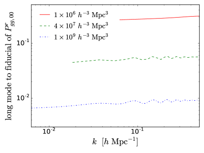
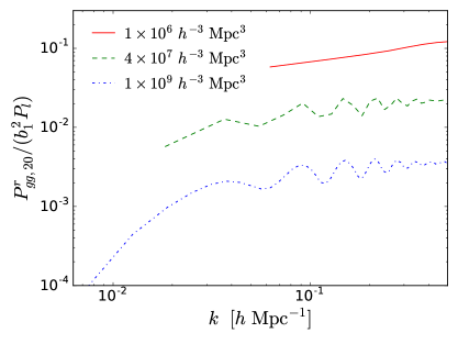
Figure 1: (Left) Ratio of the long mode contribution (terms associated with $\delta^{W}$) to fiducial ($\delta^{W}=0$) $P^{r}_{gg,00}$, which is $b_{1}^{2}P_{l}$ and independent of volume, in real space at $z=0.5$. (Right) Ratio of $P^{r}_{gg,20}$ to $b_{1}^{2}P_{l}$ in real space at $z=0.5$. The red solid, green dashed, and blue dot-dashed lines show volumes of $10^{6}$, $4\times 10^{7}$, and $10^{9}~{}h^{-3}~{}{\rm Mpc}^{3}$. The values of $\delta^{W}$ and $\mathcal{T}^{W}_{0}$ are set to be their $1-\sigma$ expected values, i.e. $\sigma_{\delta^{W}}$ and $\sigma_{\mathcal{T}^{W}_{0}}$ with spherical top-hat window function, respectively. Note that the effect of using the local mean density to compute the power spectrum, i.e. eq. (2.15) is not included.

To obtain real-space results, we can set $f=0$ in $A_{m,n}$, and the only existing components are

$$P^{r}_{gg,00}(k)=\> 2\sqrt{\pi}\Bigg{\{}\left[b_{1}^{2}+\delta^{W}\left(\frac{47}{21}b_{1}^{2}+2b_{1}b_{2}\right)\right]P_{l}(k)+\delta^{W}\left(-\frac{1}{3}b_{1}^{2}\right)P^{\prime}_{l}(k)\Bigg{\}}\,,$$

$$P^{r}_{gg,2m}(k)=\> \mathcal{T}^{W}_{m}\left[\left(\frac{8}{7}b_{1}^{2}+2b_{1}b_{s^{2}}\right)P_{l}(k)+\left(-b_{1}^{2}\right)P^{\prime}_{l}(k)\right]\,.$$

These equations have the behavior expected based on the symmetry properties of the sources: scalar sources give raise to $\ell=0$ modes and tidal $\ell=2,m$ sources give raise to $\ell=2,m$ components of the power spectrum.

The left panel of figure 1 shows the long mode contribution (terms associated with $\delta^{W}$) to fiducial ($\delta^{W}=0$ so independent of volume) $P^{r}_{gg,00}$, which is $b_{1}^{2}P_{l}$, in real space at $z=0.5$ for various volumes denoted by different colors and styles. Note that the minimum wavenumber and the density of the line reflect the corresponding volume. We set $\delta^{W}$ to be the $1-\sigma$ expected value, i.e.

$$\sigma_{\delta^{W}}=\langle(\delta^{W})^{2}\rangle^{1/2}=\left[\int d^{3}k|W(k)|^{2}P_{l}(k)\right]^{1/2}\,,$$ (2.24)

where we choose the window function to be spherical top-hat. We find that the long mode contribution is larger for smaller volume, which is the outcome of larger $\sigma_{\delta^{W}}$. We also find that the ratio is fairly scale independent, hence $\delta^{W}$ will degenerate with $b_{1}$ when performing parameter constraint and we will discuss this in details in Sec. 3. The right panel of figure 1 shows the ratio of $P^{r}_{gg,20}$ to $b_{1}^{2}P_{l}$ in real space at $z=0.5$, and as for $\delta^{W}$ we set the value of $\mathcal{T}^{W}_{0}$ to be its $1-\sigma$ expected value, which is

$$\sigma_{\mathcal{T}^{W}_{0}}=\sqrt{2}\sigma_{\mathcal{T}^{W}_{1}}=\sqrt{2}\sigma_{\mathcal{T}^{W}_{2}}=\frac{4\sqrt{\pi}}{15}\sigma_{\delta^{W}}\,.$$ (2.25)

Note that we only show the result for $P^{r}_{gg,20}$ because it has the same scale dependence as $P^{r}_{gg,21}$ and $P^{r}_{gg,22}$. Compared to the long mode contribution in $P^{r}_{gg,00}$, the signal for $P^{r}_{gg,20}$ is smaller, ranging from $\sim 10^{-4}$ to $\sim 10^{-1}$ for $V=10^{9}$ to $10^{6}~{}h^{-3}~{}{\rm Mpc}^{3}$. However, since the fiducial power spectrum does not contribute in $P^{r}_{gg,20}$, any detection of $P^{r}_{gg,20}$ is caused by the presence of $\mathcal{T}^{W}_{0}$. This opens a promising window for detecting the large-scale tide. We set the redshift to be 0.5 to match most of the current galaxy surveys, and the contribution from the long modes is smaller at high redshift, assuming that the biases are unchanged, since both $\delta^{W}$ and $\mathcal{T}^{W}_{m}$ are proportional to the linear growth factor.

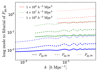
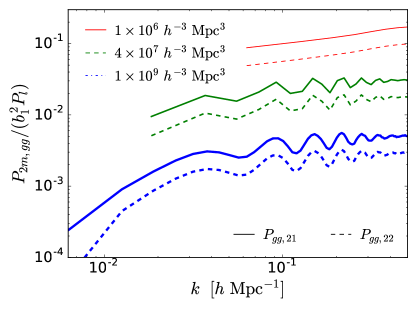
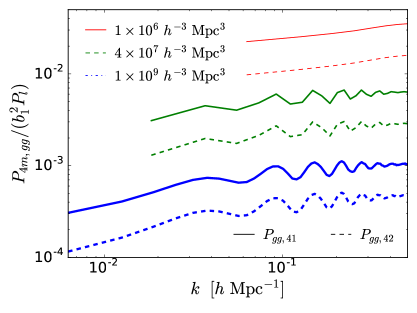
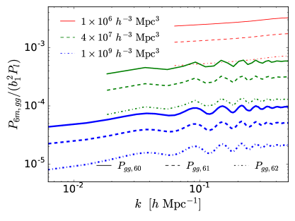
Figure 2: (Top left) Ratio of the long mode contribution (terms associated with $\delta^{W}$ and $\mathcal{T}^{W}_{0}$) to fiducial ($\delta^{W}=\mathcal{T}^{W}_{0}=0$) $P_{gg,l0}$ for $\ell\leq 4$, i.e. the Kaiser power spectrum, in redshift space at $z=0.5$. The solid, dashed, and dot-dashed lines show $\ell=0$, $2$, and $4$, respectively. The other panels show relative sizes to $b_{1}^{2}P_{l}$ of terms in redshift space at $z=0.5$ that are not sourced by the Kaiser power spectrum. (Top right) Ratio of $P_{gg,2m}$ to $b_{1}^{2}P_{l}$ for $m=1$ (solid) and 2 (dashed), which are sourced respectively by $\mathcal{T}^{W}_{1}$ and $\mathcal{T}^{W}_{2}$. (Bottom left) Same as the top right panel, but for $\ell=4$, i.e. $P_{gg,4m}$. (Bottom right) Ratio of $P_{gg,6m}$ to $b_{1}^{2}P_{l}$ for $m=0$ (solid), 1 (dashed), and 2 (dot-dashed), which are sourced respectively by $\delta^{W}$ and $\mathcal{T}^{W}_{0}$, $\mathcal{T}^{W}_{1}$, and $\mathcal{T}^{W}_{2}$. The red thin, green medium, and blue thick lines show volumes of $10^{6}$, $4\times 10^{7}$, and $10^{9}~{}h^{-3}~{}{\rm Mpc}^{3}$. The values of $\delta^{W}$ and $\mathcal{T}^{W}_{m}$ are set to be their $1-\sigma$ expected values, i.e. $\sigma_{\delta^{W}}$ and $\sigma_{\mathcal{T}^{W}_{m}}$ with spherical top-hat window function, respectively. Note that the effect of using the local mean density to compute the power spectrum, i.e. eq. (2.15) is not included.

In figure 2 we show the long mode contributions in redshift space at $z=0.5$. The top left panel shows long mode contribution (terms associated with $\delta^{W}$ and $\mathcal{T}^{W}_{0}$) to fiducial ($\delta^{W}=\mathcal{T}^{W}_{0}=0$, i.e. the Kaiser power spectrum, so independent of volume) $P_{gg,\ell 0}$ for $\ell=0$ (solid), 2 (dashed), and 4 (dot-dashed). Interestingly, we find that for $\ell=4$ and $V=10^{6}~{}h^{-3}~{}{\rm Mpc}^{3}$ the long mode contribution exceeds the fiducial Kaiser power spectrum. This indicates that it is necessary to take the long mode contribution into account for the hexadecapole of the galaxy redshift-space power spectrum when the survey volume is less than $\sim 10^{6}~{}h^{-3}~{}{\rm Mpc}^{3}$. The top right, bottom left, and bottom right panels show respectively the ratios of $P_{gg,2m}$, $P_{gg,4m}$, and $P_{gg,6m}$ to $b_{1}^{2}P_{l}$. As in real space, while these signals are smaller compared to the long mode contribution in $P_{gg,\ell 0}$, they are caused solely by the long modes ($\delta^{W}$ and $\mathcal{T}^{W}_{0}$ for $m=0$, $\mathcal{T}^{W}_{1}$ for $m=1$, and $\mathcal{T}^{W}_{2}$ for $m=2$), hence providing a great potential to probe the large-scale perturbations. Unlike in real space, the signal of the long modes depend both on the linear growth factor and the growth rate. Since the growth factor and the growth rate have opposite redshift evolutions, the long mode signal, assuming the biases do not evolve in redshift, does not have a clear redshift evolution.

Finally, we find that in general the effects of tides falls with $m$: the relative impact of $\mathcal{T}^{W}_{0}$ is larger than that of $\mathcal{T}^{W}_{1}$ which is in turn larger than that of $\mathcal{T}^{W}_{2}$. This is true in both real and redshift space.

In figure 1 and figure 2, for clarity we do not include the effect of using the local mean density to compute the power spectrum, i.e. eq. (2.15). Since the corrections have the same angular dependencies as the fiducial power spectrum, in real space the effect of the miscalibration of the mean density only contributes to terms associated with $\delta^{W}$ in $P^{r}_{gg,00}$, and in redshift space to terms associated with $\delta^{W}$ as well as $\mathcal{T}^{W}_{0}$ in $P_{gg,\ell 0}$ for $\ell=0$, 2, and 4.

2.3 Estimator and covariance

To measure $P_{gg,\ell m}(k)$ in a volume $V$, the simplest estimator is

$$\hat{P}_{gg,\ell m}(k)=\frac{4\pi}{VN(k)}\sum_{k-\Delta k/2\leq|\mathbf{k}_{i}|\leq k+\Delta k/2}\delta_{g}(\mathbf{k}_{i})\delta_{g}^{*}(\mathbf{k}_{i})Y^{*}_{\ell m}(\hat{k}_{i})\,,$$ (2.26)

where $N(k)$ is the number of independent Fourier modes. One can straightforwardly show that this estimator is unbiased because in the continuous limit

$$\frac{1}{N(k)}\sum_{k-\Delta k/2\leq|\mathbf{k}_{i}|\leq k+\Delta k/2}\to\frac{1}{4\pi}\int d^{2}\hat{k}\,.$$ (2.27)

The covariance of the estimator can be computed as

$${\rm cov}[\hat{P}_{gg,\ell m}(k),\hat{P}_{gg,\ell^{\prime}m^{\prime}}(k^{\prime})]$$

$$=\> \langle\hat{P}_{gg,\ell m}(k)\hat{P}_{gg,\ell^{\prime}m^{\prime}}(k^{\prime})\rangle-\langle\hat{P}_{gg,\ell m}(k)\rangle\langle\hat{P}_{gg,\ell^{\prime}m^{\prime}}(k^{\prime})\rangle$$

$$=\> \frac{(4\pi)^{2}}{V^{2}N(k)N(k^{\prime})}\sum_{ij}\langle\delta_{g}(\mathbf{k}_{i})\delta_{g}^{*}(\mathbf{k}^{\prime}_{j})\rangle\langle\delta_{g}^{*}(\mathbf{k}_{i})\delta_{g}(\mathbf{k}^{\prime}_{j})\rangle Y_{\ell m}^{*}(\hat{k}_{i})Y_{\ell^{\prime}m^{\prime}}^{*}(\hat{k}^{\prime}_{j})\,,$$ (2.28)

where we assume that the covariance is dominated by the disconnected Gaussian contribution and omit the full notation in the subscript of the summation. Note that $\delta^{W}$ and $\mathcal{T}^{W}_{m}$ would also contribute to the covariance [6, 7, 14, 15, 16], but we consider the survey to be large enough so that the super-sample covariance is next-to-leading order correction. One can easily see that the covariance is non-zero only if $\mathbf{k}_{i}=\mathbf{k}_{j}$, hence the covariance can be simplified to

$${\rm cov}[\hat{P}_{gg,\ell m}(k),\hat{P}_{gg,\ell^{\prime}m^{\prime}}(k)]\> =\frac{(4\pi)^{2}}{N^{2}(k)}\sum_{i}[P_{gg}(\mathbf{k}_{i})+P_{\rm shot}]^{2}Y_{\ell m}^{*}(\hat{k}_{i})Y_{\ell^{\prime}m^{\prime}}^{*}(\hat{k}_{i})$$

$$\to\frac{4\pi}{N(k)}\int d^{2}\hat{k}[P_{gg}(\mathbf{k})+P_{\rm shot}]^{2}Y_{\ell m}^{*}(\hat{k})Y_{\ell^{\prime}m^{\prime}}^{*}(\hat{k})\,,$$ (2.29)

where $P_{\rm shot}$ is the shot noise. To proceed, we assume the galaxy power spectrum is given by the Kaiser formalism, hence

$${\rm cov}[\hat{P}_{gg,\ell m}(k),\hat{P}_{gg,\ell^{\prime}m^{\prime}}(k)]\approx\frac{4\pi}{N(k)}\int d^{2}\hat{k}[(b_{1}+f\mu^{2})^{2}P_{l}(k)+P_{\rm shot}]^{2}Y_{\ell m}^{*}(\hat{k})Y_{\ell^{\prime}m^{\prime}}^{*}(\hat{k})\,,$$ (2.30)

which is non-zero only if $m=m^{\prime}$. We shall apply eq. (2.30) for the Fisher analysis in Sec. 3.

$P_{gg,\ell m}(k)$ is a complex number, and in practice we measure the real and imaginary parts separately. Thus, the covariances are

$${\rm cov}[\hat{P}_{gg,\ell m}^{R}(k),\hat{P}_{gg,\ell^{\prime}m}^{R}(k)]=\frac{4\pi}{N_{k}}\int d^{2}\hat{k}[(b_{1}+f\mu^{2})^{2}P_{l}(k)+P_{\rm shot}]^{2}{\rm Re}[Y_{\ell m}^{*}(\hat{k})]{\rm Re}[Y_{\ell^{\prime}m}^{*}(\hat{k})]\,,$$

$${\rm cov}[\hat{P}_{gg,\ell m}^{I}(k),\hat{P}_{gg,\ell^{\prime}m}^{I}(k)]=\frac{4\pi}{N_{k}}\int d^{2}\hat{k}[(b_{1}+f\mu^{2})^{2}P_{l}(k)+P_{\rm shot}]^{2}{\rm Im}[Y_{\ell m}^{*}(\hat{k})]{\rm Im}[Y_{\ell^{\prime}m}^{*}(\hat{k})]\,,$$

$${\rm cov}[\hat{P}_{gg,\ell m}^{R}(k),\hat{P}_{gg,\ell^{\prime}m}^{I}(k)]=\frac{4\pi}{N_{k}}\int d^{2}\hat{k}[(b_{1}+f\mu^{2})^{2}P_{l}(k)+P_{\rm shot}]^{2}{\rm Re}[Y_{\ell m}^{*}(\hat{k})]{\rm Im}[Y_{\ell^{\prime}m}^{*}(\hat{k})]\,,$$ (2.31)

and one can easily show that ${\rm cov}[\hat{P}_{gg,\ell m}^{R}(k),\hat{P}_{gg,\ell^{\prime}m}^{I}(k)]=0$ for all possible $\ell,m$. Therefore, the only non-zero components are

$${\rm cov}[\hat{P}_{gg,\ell m}^{R}(k),\hat{P}_{gg,\ell^{\prime}m}^{R}(k)]=\frac{4\pi}{N(k)}\int d^{2}\hat{k}[(b_{1}+f\mu^{2})^{2}P_{l}(k)+P_{\rm shot}]^{2}{\rm Re}[Y_{\ell m}^{*}(\hat{k})]{\rm Re}[Y_{\ell^{\prime}m}^{*}(\hat{k})]\,,$$

$${\rm cov}[\hat{P}_{gg,\ell m}^{I}(k),\hat{P}_{gg,\ell^{\prime}m}^{I}(k)]=\frac{4\pi}{N(k)}\int d^{2}\hat{k}[(b_{1}+f\mu^{2})^{2}P_{l}(k)+P_{\rm shot}]^{2}{\rm Im}[Y_{\ell m}^{*}(\hat{k})]{\rm Im}[Y_{\ell^{\prime}m}^{*}(\hat{k})]\,.$$ (2.32)

This means that for each $k$ the covariance matrix can be written as a block-diagonal matrix, consisting covariances of $(\hat{P}^{R}_{gg,00},\hat{P}^{R}_{gg,20},\hat{P}^{R}_{gg,40},\hat{P}^{R}_{gg,60})$, $(\hat{P}^{R}_{gg,21},\hat{P}^{R}_{gg,41},\hat{P}^{R}_{gg,61})$, $(\hat{P}^{I}_{gg,21},\hat{P}^{I}_{gg,41},\hat{P}^{I}_{gg,61})$, $(\hat{P}^{R}_{gg,22},\hat{P}^{R}_{gg,42},\hat{P}^{R}_{gg,62})$, and $(\hat{P}^{I}_{gg,22},\hat{P}^{I}_{gg,42},\hat{P}^{I}_{gg,62})$.

3 Fisher forecast

In the previous section we derive how galaxy power spectrum in a finite volume would respond to the overdensity and tidal fields with wavelengths larger than the volume. One specific example is the power spectrum in a galaxy redshift survey, and it will be affected by the super-survey modes. This also means that by measuring $P_{gg,\ell m}$ of this survey, it is possible to put constraints on the super-survey overdensity and tidal fields, which are usually not directly observable unless a large survey containing the current one is performed.

To explore the ability of measuring the long mode for a given survey, we apply the Fisher matrix as

$$F_{\alpha\beta}=\sum_{k=k_{\rm min}}^{k_{\rm max}}\sum_{\ell\ell^{\prime}}\sum_{m}\left[{\rm cov}[P_{gg,\ell m}(k),P_{gg,\ell^{\prime}m}(k)]\right]^{-1}\frac{\partial P_{gg,\ell m}(k)}{\partial\theta_{\alpha}}\frac{\partial P_{gg,\ell^{\prime}m}(k)}{\partial\theta_{\beta}}\,,$$ (3.1)

where $\theta_{\alpha}$ is the parameter of interest. The constraint on $\theta_{\alpha}$ as well as the correlation between $\theta_{\alpha}$ and $\theta_{\beta}$ are then

$${\rm err}[\theta_{\alpha}]=\sqrt{\left(F^{-1}\right)_{\alpha\alpha}}\,,\quad{\rm corr}[\theta_{\alpha},\theta_{\beta}]=\frac{\left(F^{-1}\right)_{\alpha\beta}}{{\rm err}[\theta_{\alpha}]{\rm err}[\theta_{\beta}]}\,.$$ (3.2)

For the fitting range we set $k_{\rm min}=k_{F}$ to be the fundamental frequency of survey and explore the constraint for different $k_{\rm max}$. In this paper we shall adopt the Planck cosmology [26], i.e. $h=0.6803$, $\Omega_{b}h^{2}=0.0226$, $\Omega_{c}h^{2}=0.1186$, $A_{s}=2.137\times 10^{-9}$, and $n_{s}=0.9667$, hence the shape of the power spectrum is fixed. We fix the redshift to be 0.5 because it is the redshift at which most galaxy surveys are performed, but the results can be straightforwardly generalized to other redshifts. The parameters of interest are $\theta_{\alpha}\in(b_{1},b_{2},b_{s^{2}},f,\delta^{W},\mathcal{T}^{W}_{0},\mathcal{T}^{W,R}_{1},\mathcal{T}^{W,I}_{1},\mathcal{T}^{W,R}_{2},\mathcal{T}^{W,I}_{2})$, where $\mathcal{T}^{W}_{1}$ and $\mathcal{T}^{W}_{2}$ are complex numbers so there are four parameters in total that one can measure. We set the fiducial values of the biases and growth rate to be $b_{1}=2$, $b_{2}=0.3$, $b_{s^{2}}=-\frac{4}{7}(b_{1}-1)=-0.57$, and $f(z=0.5)=0.75$, and for the long mode we set the fiducial value to be the $1-\sigma$ expected value for the corresponding volume, assuming a spherical top-hat window function. In the following we shall separately discuss the results in real and redshift space, and in real space we set $f=0$ so the number of parameters is nine.

3.1 Real space

Let us begin with the Fisher analysis in real space, in which the power spectra are given in eq. (LABEL:eq:Pggr). Moreover, since the global mean density is unknown if only a finite survey is performed, only the local mean density can be used to measure the power spectrum, hence there is an additional contribution to the response from the miscalibration of the mean density. We thus use eq. (2.15) to mimic this effect, and only $P^{r}_{gg,00}$ contains the additional contribution.

We first notice that Fisher matrix is not positive definite. This happens because there are nine parameters to be determined, but from eq. (LABEL:eq:Pggr) one can only measure eight scale dependencies: two from $P^{r}_{gg,00}$, two from $P^{r}_{gg,20}$, and two from $P^{r}_{gg,21}$ and $P^{r}_{gg,22}$ respectively because they are complex numbers and have the same scale dependence as $P^{r}_{gg,20}$ hence only four independent amplitudes can be measured. Since the main focus of this paper is to probe the long mode as well as to study their impact on $b_{1}$ and $f$, we shall include priors of $\pm 1$ on $b_{2}$ and $b_{s^{2}}$. These priors are sufficiently strong that they break the perfect degeneracy to the extent that more constraining prior has negligible effects on the results.

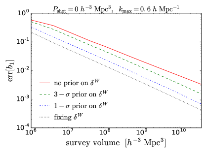
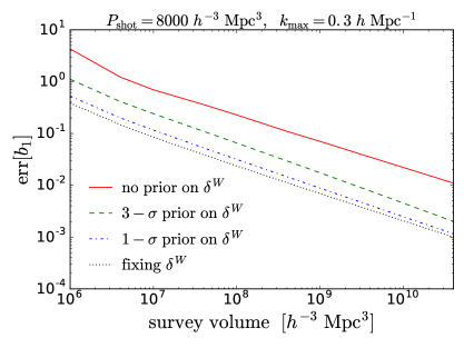
Figure 3: $1-\sigma$ constraint on $b_{1}$ from the real-space galaxy power spectrum as a function of survey volume for two $P_{\rm shot}$ and $k_{\rm max}$. The left panel shows a cosmic variance limited survey with high $k_{\rm max}$, whereas the right panel shows a BOSS-like survey number density with a realistic $k_{\rm max}$. Lines with different colors and styles show various priors on $\delta^{W}$. Note that a large number of $\sigma$ is for a weaker prior.

Adding priors to $b_{2}$ and $b_{s^{2}}$, the Fisher matrix becomes invertible, and we find that $b_{1}$ and $\delta^{W}$ are highly correlated. Specifically, for $10^{6}\leq V/(h^{-3}~{}{\rm Mpc}^{3})\leq 4\times 10^{10}$, $0\leq P_{\rm shot}/(h^{-3}~{}{\rm Mpc}^{3})\leq 8000$ (cosmic variance limited to the BOSS-like survey number density [27]), and $0.1\leq k_{\rm max}/(h~{}{\rm Mpc}^{-1})\leq 0.5$, the correlation between $b_{1}$ and $\delta^{W}$ is greater than 0.95. The large correlation is not surprising as the ratio shown in the left panel of figure 1 is quite scale independent, and the correction from the miscalibration of the mean density has identical scale dependence as the fiducial power spectrum. This means that the constraint on $b_{1}$ will be largely determined by the knowledge on $\delta^{W}$. Figure 3 shows the $1-\sigma$ constraint on $b_{1}$ as a function of survey volume for two $P_{\rm shot}$ and $k_{\rm max}$: the left panel shows no shot noise whereas the right panel shows a BOSS-like survey number density. It is evident that the constraint on $b_{1}$ is largely dominated by the prior on $\delta^{W}$. Specifically, adding a $1-\sigma$ prior on $\delta^{W}$ can improve the constraint on $b_{1}$ by an order of magnitude compared to no prior. The main caveat in figure 3 is that we only consider the leading-order galaxy power spectrum, and in reality the small-scale nonlinearities in matter power spectrum and galaxy bias reduce the information on linear bias. Nevertheless, figure 3 clearly demonstrates the impact from the knowledge of $\delta^{W}$ on $b_{1}$ constraint.

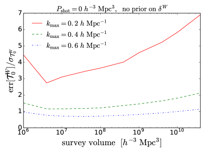
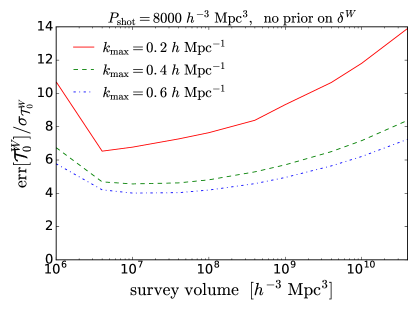
Figure 4: Ratio of the $1-\sigma$ constraint on $\mathcal{T}^{W}_{0}$ to its expected value, i.e. ${\rm err}[\mathcal{T}^{W}_{0}]/\sigma_{\mathcal{T}^{W}_{0}}$, as a function of survey volume for $P_{\rm shot}=0$ (left) and $8000~{}h^{-3}~{}{\rm Mpc}^{3}$ (right). The red solid, green dashed, and blue dot-dashed lines show respectively $k_{\rm max}=0.2$, 0.4, and $0.6~{}h~{}{\rm Mpc}^{-1}$, whereas the black dotted line is for $\sigma_{\mathcal{T}^{W}_{0}}$. We do not include any prior on $\delta^{W}$, as it has negligible impact on the constraint on $\mathcal{T}^{W}_{0}$. Furthermore, we only present the constraint on $\mathcal{T}^{W}_{0}$ because the results are identical for $\mathcal{T}^{W,R}_{1}$, $\mathcal{T}^{W,I}_{1}$, $\mathcal{T}^{W,R}_{2}$, and $\mathcal{T}^{W,I}_{2}$.

For the large-scale tidal fields, we find that the absolute value of the correlation between $b_{1}$ and $\mathcal{T}^{W}_{m}$ is less than 0.1 if the survey volume is greater than $10^{8}~{}h^{-3}~{}{\rm Mpc}^{3}$. The reason is that the constraint on $b_{1}$ is mainly from $P^{r}_{gg,00}$, for which $\mathcal{T}^{W}_{m}$ do not contribute. As a result, the prior on $\delta^{W}$ has negligible effect on the constraints on $\mathcal{T}^{W}_{m}$, meaning that $\mathcal{T}^{W}_{m}$ can be measured robustly in real space. Figure 4 shows the ratio of the $1-\sigma$ constraint on $\mathcal{T}^{W}_{0}$ to its expected value, i.e. ${\rm err}[\mathcal{T}^{W}_{0}]/\sigma_{\mathcal{T}^{W}_{0}}$, as a function of survey volume for $P_{\rm shot}=0$ (left) and $8000~{}h^{-3}~{}{\rm Mpc}^{3}$ (right). We only present the constraint on $\mathcal{T}^{W}_{0}$ since the results are identical for $\mathcal{T}^{W,R}_{1}$, $\mathcal{T}^{W,I}_{1}$, $\mathcal{T}^{W,R}_{2}$, and $\mathcal{T}^{W,I}_{2}$. The red solid, green dashed, and blue dot-dashed lines show respectively $k_{\rm max}=0.2$, 0.4, and $0.6~{}h~{}{\rm Mpc}^{-1}$. We find that the constraint depends significantly on the shot noise. Specifically, for the cosmic variance limited survey ($P_{\rm shot}=0$) $\sigma_{\mathcal{T}^{W}_{0}}$ can be achieved if $k_{\rm max}=0.6~{}h~{}{\rm Mpc}^{-1}$, while for BOSS-like survey number density the constraint on $\sigma_{\mathcal{T}^{W}_{0}}$ worsen by more than a factor of two. Note that while it may seem unrealistic to adopt $k_{\rm max}=0.6~{}h~{}{\rm Mpc}^{-1}$ for a galaxy redshift survey, the presence of $P^{r}_{gg,2m}$ cannot be produced by nonlinear evolution and is a distinct feature of large-scale tidal fields. Therefore, in the spirit of putting an upper limit on $\mathcal{T}^{W}_{m}$, it is justified to use much higher wavenumber. Moreover, on small scales the survey window function tends to be isotropized [28], hence the contamination on $P^{r}_{gg,2m}$ due to the survey window function becomes less important [25]. In figure 4 we also notice a minimum ratio at $\sim 3\times 10^{6}~{}h^{-3}~{}{\rm Mpc}^{3}$. This is because for small volume the signal due to $\mathcal{T}^{W}_{m}$ is larger and for large volume there are more modes one can access to constrain $\mathcal{T}^{W}_{m}$. Hence there is a sweet spot in the survey volume for constraining the large-scale tidal fields, and the exact value depends on $P_{\rm shot}$ and $k_{\rm max}$.

3.2 Redshift space

Let us now turn to the Fisher analysis in redshift space, in which the power spectra are given in eqs. (2.20)–(2.22) with ten parameters. As in real space, we adopt eq. (2.15) to account for the miscalibration of the mean density when measuring the power spectrum in a finite survey, so $P_{gg,00}$, $P_{gg,20}$, and $P_{gg,40}$ receive additional contribution. To make the inversion of the Fisher matrix stable, we also include a prior of $\pm 1$ on $b_{2}$ and $b_{s^{2}}$. Since the conclusions are insensitive to the choice of the survey parameters, in this section we shall fix $P_{\rm shot}=8000~{}h^{-3}~{}{\rm Mpc}^{3}$ and $k_{\rm max}=0.3~{}h~{}{\rm Mpc}^{-1}$ for a more realistic forecast.

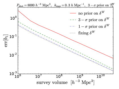
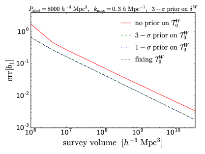
Figure 5: (Left) $1-\sigma$ constraint on $b_{1}$ from the redshift-space galaxy power spectrum as a function of survey volume for $P_{\rm shot}=8000~{}h^{-3}~{}{\rm Mpc}^{3}$, $k_{\rm max}=0.3~{}h~{}{\rm Mpc}^{-1}$, and a $3-\sigma$ prior on $\mathcal{T}^{W}_{0}$. Lines with different colors and styles show various priors on $\delta^{W}$. (Right) Same as the left panel, but with a $3-\sigma$ prior on $\delta^{W}$. Lines with different colors and styles show various priors on $\mathcal{T}^{W}_{0}$.

We first examine the constraint on $b_{1}$, which is dominated by $P_{gg,00}$, $P_{gg,20}$, and $P_{gg,40}$ due to their large signal-to-noise ratios compared to the rest of $P_{gg,\ell m}$. Since only $\delta^{W}$ and $\mathcal{T}^{W}_{0}$ contribute to $m=0$ components, we expect that $b_{1}$ is mostly degenerate with them. As in real space, we find that $b_{1}$ and $\delta^{W}$ are highly correlated regardless of the survey parameters and the priors on $\mathcal{T}^{W}_{m}$, with correlation coefficients greater than 0.8, hence the constraint on $b_{1}$ will depend strongly on the prior on $\delta^{W}$. The left panel of figure 5 shows the $1-\sigma$ constraint on $b_{1}$ from the redshift-space galaxy power spectrum with a $3-\sigma$ prior on $\mathcal{T}^{W}_{0}$ as a function of survey volume. We find that different priors on $\delta^{W}$ can affect the constraint on $b_{1}$ by more than an order of magnitude, and this finding is consistent as in real space. For the correlation coefficient between $b_{1}$ and $\mathcal{T}^{W}_{0}$, we find it to be less than -0.5 when no prior on $\delta^{W}$ is included. The anti-correlation increases when we include a prior on $\delta^{W}$, hence we expect to see some dependence on the prior on $\mathcal{T}^{W}_{0}$ of the constraint on $b_{1}$. The right panel of figure 5 shows the $1-\sigma$ constraint on $b_{1}$ with a $3-\sigma$ prior on $\delta^{W}$. We find that as long as there is some prior on $\mathcal{T}^{W}_{0}$, the constraint on $b_{1}$ converges well, indicating that a reliable constraint on $b_{1}$ can be obtained even with a conservative ($3-\sigma$) prior on $\mathcal{T}^{W}_{0}$. Interestingly, we notice that if there is no prior on $\delta^{W}$, then the prior on $\mathcal{T}^{W}_{0}$ has negligible effect on the constraint on $b_{1}$. This further reinforces the strong correlation between $b_{1}$ and $\delta^{W}$.

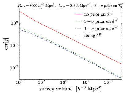
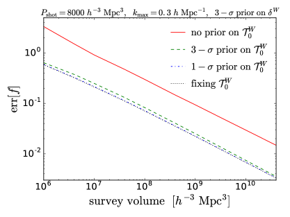
Figure 6: (Left) 1-$\sigma$ constraint on $f$ from the redshift-space galaxy power spectrum as a function of survey volume for $P_{\rm shot}=8000~{}h^{-3}~{}{\rm Mpc}^{3}$, $k_{\rm max}=0.3~{}h~{}{\rm Mpc}^{-1}$, and a $3-\sigma$ prior on $\mathcal{T}^{W}_{0}$. Lines with different colors and styles show various priors on $\delta^{W}$. (Right) Same as the left panel, but with a $3-\sigma$ prior on $\delta^{W}$. Lines with different colors and styles show various priors on $\mathcal{T}^{W}_{0}$.

We next examine the constraint on $f$, which as $b_{1}$ is dominated by $P_{gg,00}$, $P_{gg,20}$, and $P_{gg,40}$, so we focus on the degeneracy with $\delta^{W}$ and $\mathcal{T}^{W}_{0}$ as well. We find that the absolute value of the correlation coefficient between $f$ and $\delta^{W}$ is less than 0.35 (weaker correlation for larger volume) and has almost no dependence on the prior on $\mathcal{T}^{W}_{0}$, whereas the correlation coefficient between $f$ and $\mathcal{T}^{W}_{0}$ changes from $\sim-0.85$ for no prior on $\delta^{W}$ to less than -0.9 for a conservative $3-\sigma$ prior on $\delta^{W}$. The strong effect suggests that the constraint on $f$ will be dependent on both the priors on $\delta^{W}$ and $\mathcal{T}^{W}_{0}$, and indeed we find that just adding one prior on either $\delta^{W}$ or $\mathcal{T}^{W}_{0}$ does not improve the constraint on $f$. Figure 6 shows the constraint on $f$ from the redshift-space galaxy power spectrum with various priors on $\delta^{W}$ and $\mathcal{T}^{W}_{0}$ as a function of the survey volume. Including conservative $3-\sigma$ priors on both $\delta^{W}$ and $\mathcal{T}^{W}_{0}$ reduces the constraint on $f$ significantly compared to the one with only one prior on either $\delta^{W}$ or $\mathcal{T}^{W}_{0}$, and the result converges well with that of fixing both $\delta^{W}$ and $\mathcal{T}^{W}_{0}$. This implies that for future large-scale structure analysis it is sufficient to obtain a rigorous constraint on $f$ as long as $3-\sigma$ priors on both $\delta^{W}$ and $\mathcal{T}^{W}$ are added.

Since $b_{1}$ and $f$ are mostly degenerate with $\delta^{W}$ and $\mathcal{T}^{W}_{0}$, it is natural to ask whether the inclusion of $P_{gg,60}$, which can only be produced by $\delta^{W}$ and $\mathcal{T}^{W}_{0}$, improves the constraint on $b_{1}$ and $f$ or not. To address this question, we perform the Fisher analysis using the observables of $(P_{gg,00},P_{gg,20},P_{gg,40})$ and $(P_{gg,00},P_{gg,20},P_{gg,40},P_{gg,60})$. However, we find that the constraint on $b_{1}$ and $f$ is insensitive to the presence of $P_{gg,60}$. This is likely due to the low signal-to-noise ratio of $P_{gg,60}$, because even if $\delta^{W}$ ($\mathcal{T}^{W}_{0}$) is fixed, the constraint on $\mathcal{T}^{W}_{0}$ ($\delta^{W}$) reduces only by a few percent regardless of the existence of $P_{gg,60}$. Therefore, it is better to include priors on $\delta^{W}$ and $\mathcal{T}^{W}_{0}$ for acquiring reliable constraints on both $b_{1}$ and $f$.

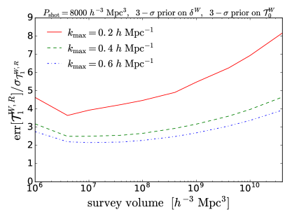
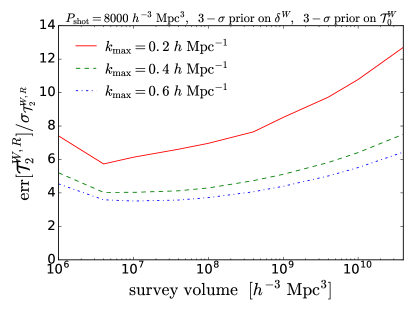
Figure 7: (Left) Ratio of the 1-$\sigma$ constraint from the galaxy redshift-space power spectrum on $\mathcal{T}^{W,R}_{1}$ to its expected value, i.e. ${\rm err}[\mathcal{T}^{W,R}_{1}]/\sigma_{\mathcal{T}^{W,R}_{1}}$, as a function of survey volume for $P_{\rm shot}=8000~{}h^{-3}~{}{\rm Mpc}^{3}$, and $3-\sigma$ priors on $\delta^{W}$ and $\mathcal{T}^{W}_{0}$. The constraint on $\mathcal{T}^{W,I}_{1}$ is identical to $\mathcal{T}^{W,R}_{1}$. Lines with different colors and styles show various $k_{\rm max}$. (Right) Same as the left panel, but for the $1-\sigma$ constraint on $\mathcal{T}^{W,R}_{2}$.

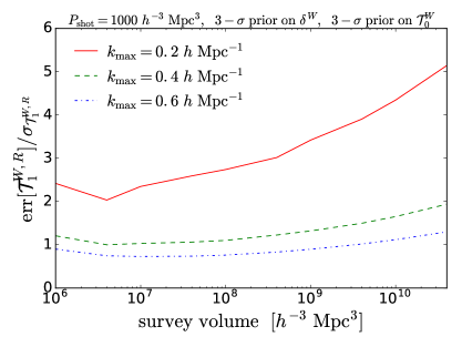
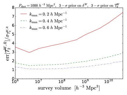
Figure 8: Same as figure 7, but with $P_{\rm shot}=1000~{}h^{-3}~{}{\rm Mpc}^{3}$.

While it is difficult to measure $\delta^{W}$ and $\mathcal{T}^{W}_{0}$ due to their low signal-to-noise, $\mathcal{T}^{W}_{1}$ and $\mathcal{T}^{W}_{2}$ can be probed because they are the only sources that can contribute respectively to $P_{gg,\ell 1}$ and $P_{gg,\ell 2}$. Moreover, we find that for a survey volume greater than $10^{8}~{}h^{-3}~{}{\rm Mpc}^{3}$, the absolute values of the correlation coefficients between $b_{1}$ and $\mathcal{T}^{W}_{m}$ as well as $f$ and $\mathcal{T}^{W}_{m}$ are less than 0.1 for $m\geq 1$. Figure 7 shows the ratios of the $1-\sigma$ constraints from the redshift-space galaxy power spectrum on $\mathcal{T}^{W,R}_{1}$ (left) and $\mathcal{T}^{W,R}_{2}$ (right) to their expected values, i.e. ${\rm err}[\mathcal{T}^{W,R}_{1}]/\sigma_{\mathcal{T}^{W,R}_{1}}$ and ${\rm err}[\mathcal{T}^{W,R}_{2}]/\sigma_{\mathcal{T}^{W,R}_{2}}$, as a function of survey volume for $P_{\rm shot}=8000~{}h^{-3}~{}{\rm Mpc}^{3}$, and $3-\sigma$ priors on $\delta^{W}$ and $\mathcal{T}^{W}_{0}$. The constraints on the imaginary part are identical to the real part. We find that although it is possible to put upper bounds on the super-survey tidal fields, the constraints are quite weak, ranging from $\sim 3$ to 4 times of the $\Lambda$CDM expected values for a survey of $10^{9}~{}h^{-3}~{}{\rm Mpc}^{3}$, even if a large $k_{\rm max}$ of $0.6~{}h~{}{\rm Mpc}^{-1}$ is used. The weak constraints are mainly driven by the large shot noise, and for a high number density survey with $P_{\rm shot}=1000~{}h^{-3}~{}{\rm Mpc}^{3}$ as shown in figure 8, one can in general put $\sim 1-\sigma$ constraints on the super-survey tidal fields as long as a high $k_{\rm max}$ is adopted. This is consistent with the finding in Ref. [15] when all cosmological parameters are fixed, though they only forecasted the constraint for $\mathcal{T}^{W}_{0}$.

4 Conclusion

We have generalized the Kaiser formula in a finite volume with large-scale overdensity and tidal fields. We find that $\ell=0,2,4,6$ and $m=0,1,2$ modes are present in spherical harmonic expansion. The linear power spectrum and mean overdensity generate the azimuthally symmetric $\ell=0,2,4,6$, $m=0$ modes of the power spectrum. The tidal fields, written as a quadrupole, generate $\ell=2,4,6$ modes of the power spectrum, separately for each $m$ components. Hence, the azimuthal symmetry of the Kaiser power spectrum in a finite volume is broken due to the presence of the large-scale tidal fields.

The first non-trivial result of writing equations in this way is that we note that the tidal contribution to the azimuthally symmetric power spectrum is sourced by just one of the five degrees of freedom present in the tidal fields. This allows a more natural way of marginalizing over this uncertainty. Our numerical calculation shows that the relative size of effect associated with the tidal fields decrease with increasing $m$.

The additional small-scale physics cannot break the basic symmetries of the problem. Hence, beyond second order physics that is still linear in $\mathcal{T}^{W}_{m}$ will only affect the same $m$ modes, although it can in principle affect arbitrarily large $\ell$, for example, fingers of God. However, terms that are quadratic in $\mathcal{T}^{W}_{m}$ will in general couple to the sum and difference of two $m$ components.

As a concrete example, we made Fisher forecasts for a galaxy redshift survey in determining the galaxy bias parameters, the growth rate $f$, and the super-survey overdensity $\delta^{W}$ and tidal fields $\mathcal{T}^{W}_{m}$. While fitting and marginalizing over $\mathcal{T}^{W}_{0}$ and $\delta^{W}$ is an efficient way of dealing with the super-sample covariance [6, 7], using the power spectrum components of $m>0$ one can directly probe the super-sample tidal fields, that are usually not directly observable unless a larger volume containing the current survey is observed.

Our numerical work also shows that $\delta^{W}$ and linear bias are highly degenerate, as expected. For measuring tidal fields, we find a shallow optimum survey size that is given by two competing effects: increasing volume increases the precision with which we can measure the power spectrum but at the same time decreases the expected signal of the super-sample modes. The optimum is at around $V\sim 3\times 10^{7}~{}h^{-3}~{}{\rm Mpc}^{3}$ and depends only weakly on the number density involved. However, in general we find that the constraint on the tidal fields depends strongly on the galaxy number density, and for a realistic survey the signal-to-noise ratio is generally below unity, indicating that it is challenging to probe the super-sample tidal fields by measuring the anisotropic galaxy power spectrum. On the other hand, for a high number density galaxy survey ($P_{\rm shot}=1000~{}h^{-3}~{}{\rm Mpc}^{3}$) it is possible to put $\sim 1-\sigma$ constraints on the super-survey tidal fields of $\mathcal{T}^{W}_{1}$ and $\mathcal{T}^{W}_{2}$ at their $\Lambda$CDM expected values. Finally, it is logically possible that when measured, the measured tidal field would turn up to be considerably larger than expected, perhaps due to new physics at the horizon scale. Our result indicates that if the actual tidal fields are no more than an order of magnitude larger than expected value, they are likely to be measurable with high significance.

When this technique is applied to a real survey, the curvature of the sky and shape of the actual window survey would need to be taken into account carefully. For a fixed large-scale tide, the tidal tensor will be rotated with respect to the line of sight across a survey covering large fraction of the sky. A correct methodology for dealing with this exceeds the scope of this paper.

Another way to probe the super-volume tidal fields is to divide the entire survey into smaller subvolumes and measure the fully anisotropic power spectrum in each subvolume, as the position-dependent power spectrum approach [8, 22]. In this way, one measures the tidal fields with scale larger than the subvolume size but smaller than the entire survey, hence the signal-to-noise is expected to be much higher compared to the super-survey modes. Since the effect of the long mode on the large-scale overdensity and tidal fields is equivalent to the squeezed bispectrum, the same information can also be extracted from full bispectrum measurements. However, there are now numerically highly efficient methods for bispectrum measurements [29, 30, 31] that make the measurements based on subvolume power spectrum variations likely obsolete.

Appendix A Angular decomposition of redshift-space galaxy power spectrum in the presence of long-wavelength overdensity and tide

From eqs. (2.10)–(2.11), it is straightforward to find

$$A_{0,0}=\left(b_{1}^{2}\right)P_{l}(k)\,,\quad A_{0,1}=\left(2b_{1}f\right)P_{l}(k)\,,\quad A_{0,2}=\left(f^{2}\right)P_{l}(k)\,,$$

$$A_{1,0}=\left(\frac{47}{21}b_{1}^{2}+2b_{1}b_{2}+\frac{1}{3}b_{1}^{2}f\right)P_{l}(k)+\left(-\frac{1}{3}b_{1}^{2}\right)P^{\prime}_{l}(k)\,,$$

$$A_{1,1}=\left(\frac{26}{7}b_{1}f+2b_{1}^{2}f+2b_{2}f\right)P_{l}(k)+\left(-\frac{2}{3}b_{1}f-\frac{1}{3}b_{1}^{2}f\right)P^{\prime}_{l}(k)\,,$$

$$A_{1,2}=\left(\frac{31}{21}f^{2}+\frac{10}{3}b_{1}f^{2}-\frac{1}{3}f^{3}\right)P_{l}(k)+\left(-\frac{1}{3}f^{2}-\frac{2}{3}b_{1}f^{2}\right)P^{\prime}_{l}(k)\,,$$

$$A_{1,3}=\left(\frac{4}{3}f^{3}\right)P_{l}(k)+\left(-\frac{1}{3}f^{3}\right)P^{\prime}_{l}(k)\,,\quad A_{2,0}=\left(\frac{8}{7}b_{1}^{2}+2b_{1}b_{s^{2}}\right)P_{l}(k)+\left(-b_{1}^{2}\right)P^{\prime}_{l}(k)\,,$$

$$A_{2,1}=\left(\frac{24}{7}b_{1}f+2b_{s^{2}}f\right)P_{l}(k)+\left(-2b_{1}f\right)P^{\prime}_{l}(k)\,,\quad A_{2,2}=\left(\frac{16}{7}f^{2}\right)P_{l}(k)+\left(-f^{2}\right)P^{\prime}_{l}(k)\,,$$

$$A_{3,0}=\left(-b_{1}^{2}f\right)P^{\prime}_{l}(k)\,,\quad A_{3,1}=\left(4b_{1}f^{2}\right)P_{l}(k)+\left(-2b_{1}f^{2}\right)P^{\prime}_{l}(k)\,,$$

$$A_{3,2}=\left(4f^{3}\right)P_{l}(k)+\left(-f^{3}\right)P^{\prime}_{l}(k)\,,\quad A_{4,0}=\left(b_{1}^{2}f\right)P_{l}(k)\,,\quad A_{4,1}=\left(-f^{3}\right)P_{l}(k)\,.$$ (A.1)

References

- [1] N. Kaiser, Clustering in real space and in redshift space, Mon. Not. Roy. Astron. Soc. 227 (1987) 1–27.
- [2] M. Shiraishi, N. S. Sugiyama and T. Okumura, Polypolar spherical harmonic decomposition of galaxy correlators in redshift space: Toward testing cosmic rotational symmetry, Phys. Rev. D95 (2017) 063508, [1612.02645].
- [3] F. Bernardeau, S. Colombi, E. Gaztanaga and R. Scoccimarro, Large scale structure of the universe and cosmological perturbation theory, Phys. Rept. 367 (2002) 1–248, [astro-ph/0112551].
- [4] F. Schmidt, E. Pajer and M. Zaldarriaga, Large-Scale Structure and Gravitational Waves III: Tidal Effects, Phys. Rev. D89 (2014) 083507, [1312.5616].
- [5] K. Osato, T. Nishimichi, M. Oguri, M. Takada and T. Okumura, Strong orientation dependence of surface mass density profiles of dark haloes at large scales, 1712.00094.
- [6] Y. Li, W. Hu and M. Takada, Super-Sample Covariance in Simulations, Phys. Rev. D89 (2014) 083519, [1401.0385].
- [7] Y. Li, W. Hu and M. Takada, Super-Sample Signal, Phys. Rev. D90 (2014) 103530, [1408.1081].
- [8] C.-T. Chiang, C. Wagner, F. Schmidt and E. Komatsu, Position-dependent power spectrum of the large-scale structure: a novel method to measure the squeezed-limit bispectrum, JCAP 1405 (2014) 048, [1403.3411].
- [9] C. Wagner, F. Schmidt, C.-T. Chiang and E. Komatsu, The angle-averaged squeezed limit of nonlinear matter N-point functions, JCAP 1508 (2015) 042, [1503.03487].
- [10] C.-T. Chiang, Halo squeezed-limit bispectrum with primordial non-Gaussianity: A power spectrum response approach, Phys. Rev. D95 (2017) 123517, [1701.03374].
- [11] L. Dai, E. Pajer and F. Schmidt, On Separate Universes, JCAP 1510 (2015) 059, [1504.00351].
- [12] A. Barreira and F. Schmidt, Responses in Large-Scale Structure, JCAP 1706 (2017) 053, [1703.09212].
- [13] T. Nishimichi and P. Valageas, Redshift-space equal-time angular-averaged consistency relations of the gravitational dynamics, Phys. Rev. D92 (2015) 123510, [1503.06036].
- [14] K. Akitsu, M. Takada and Y. Li, Large-scale tidal effect on redshift-space power spectrum in a finite-volume survey, Phys. Rev. D95 (2017) 083522, [1611.04723].
- [15] K. Akitsu and M. Takada, Impact of large-scale tides on cosmological distortions via redshift-space power spectrum, Phys. Rev. D97 (2018) 063527, [1711.00012].
- [16] Y. Li, M. Schmittfull and U. Seljak, Galaxy power-spectrum responses and redshift-space super-sample effect, JCAP 1802 (2018) 022, [1711.00018].
- [17] H. Y. Ip and F. Schmidt, Large-Scale Tides in General Relativity, JCAP 1702 (2017) 025, [1610.01059].
- [18] A. S. Schmidt, S. D. M. White, F. Schmidt and J. Stücker, Cosmological N-Body Simulations with a Large-Scale Tidal Field, 1803.03274.
- [19] U.-L. Pen, R. Sheth, J. Harnois-Deraps, X. Chen and Z. Li, Cosmic Tides, 1202.5804.
- [20] H.-M. Zhu, U.-L. Pen, Y. Yu, X. Er and X. Chen, Cosmic tidal reconstruction, Phys. Rev. D93 (2016) 103504, [1511.04680].
- [21] H.-M. Zhu, U.-L. Pen, Y. Yu and X. Chen, Recovering lost 21-cm radial modes for cross correlation with the CMB and photo-z galaxies via cosmic tidal reconstruction, 1610.07062.
- [22] C.-T. Chiang, C. Wagner, A. G. Sánchez, F. Schmidt and E. Komatsu, Position-dependent correlation function from the SDSS-III Baryon Oscillation Spectroscopic Survey Data Release 10 CMASS Sample, JCAP 1509 (2015) 028, [1504.03322].
- [23] V. Desjacques, D. Jeong and F. Schmidt, Large-Scale Galaxy Bias, Phys. Rept. 733 (2018) 1–193, [1611.09787].
- [24] C.-T. Chiang and A. Slosar, The Lyman- power spectrum—CMB lensing convergence cross-correlation, JCAP 1801 (2018) 012, [1708.07512].
- [25] N. S. Sugiyama, M. Shiraishi and T. Okumura, Limits on statistical anisotropy from BOSS DR12 galaxies using bipolar spherical harmonics, Mon. Not. Roy. Astron. Soc. 473 (2018) 2737–2752, [1704.02868].
- [26] Planck collaboration, P. A. R. Ade et al., Planck 2015 results. XIII. Cosmological parameters, Astron. Astrophys. 594 (2016) A13, [1502.01589].
- [27] BOSS collaboration, S. Alam et al., The clustering of galaxies in the completed SDSS-III Baryon Oscillation Spectroscopic Survey: cosmological analysis of the DR12 galaxy sample, Mon. Not. Roy. Astron. Soc. 470 (2017) 2617–2652, [1607.03155].
- [28] T. Sato, G. Hütsi, G. Nakamura and K. Yamamoto, Window effect in the power spectrum analysis of a galaxy redshift survey, Int. J. Astron. Astrophys. 3 (2013) 243–256, [1308.3551].
- [29] M. Schmittfull, T. Baldauf and U. Seljak, Near optimal bispectrum estimators for large-scale structure, Phys. Rev. D91 (2015) 043530, [1411.6595].
- [30] R. Scoccimarro, Fast Estimators for Redshift-Space Clustering, Phys. Rev. D92 (2015) 083532, [1506.02729].
- [31] N. S. Sugiyama, S. Saito, F. Beutler and H.-J. Seo, A complete FFT-based decomposition formalism for the redshift-space bispectrum, 1803.02132.