High-order Finite Element–Integral Equation Coupling on Embedded Meshes

Abstract

This paper presents a high-order method for solving an interface problem for the Poisson equation on embedded meshes through a coupled finite element and integral equation approach. The method is capable of handling homogeneous or inhomogeneous jump conditions without modification and retains high-order convergence close to the embedded interface. We present finite element-integral equation (FE-IE) formulations for interior, exterior, and interface problems. The treatments of the exterior and interface problems are new. The resulting linear systems are solved through an iterative approach exploiting the second-kind nature of the IE operator combined with algebraic multigrid preconditioning for the FE part. Assuming smooth continuations of coefficients and right-hand-side data, we show error analysis supporting high-order accuracy. Numerical evidence further supports our claims of efficiency and high-order accuracy for smooth data.

1 Introduction

The focus of this work is on the following model interface problem for the Poisson equation:

(1a) $$-\triangle u(x) =\,f(x) \Omega^{i}\cup\Omega^{e}$$ in

(1b) $$u^{i}(x) =\,cu^{e}(x)+a(x) \Gamma$$ on

(1c) $$\frac{\partial u^{i}(x)}{\partial n} =\,\kappa\frac{\partial u^{e}(x)}{\partial n}+b(x) \textnormal{on $\Gamma$},$$

where two bounded domains $\Omega^{i},\Omega^{e}\subset\mathbb{R}^{d}$ are separated by an interface $\Gamma=\bar{\Omega}^{i}\cap\bar{\Omega}^{e}$ so that $\partial\Omega^{i}=\Gamma$. The restriction of $u$ to domain $\Omega^{\alpha}$ is written as $u^{\alpha}$ ($\alpha\in\{i,e\}$). We assume $\Omega^{i}$ has a smooth boundary. Example domains are illustrated in Figure 1. The forcing function $f$ may be discontinuous across $\Gamma$, provided smooth extensions are available in a large enough region across $\Gamma$, as discussed in more detail in Section 2. General interface problems of this kind describe, e.g., steady-state diffusion in multiple-material domains, and are closely related to problems from multi-phase low Reynolds number flow, such as viscous drop deformation and breakup [1]. The presented method is usable and much of the related analysis are valid in two or three dimensions. Numerical experiments in two dimensions support the validity of our claims; experiments in three dimensions are the subject of future investigation.

Figure 1: Two domains, $\Omega^{i}$ and $\Omega^{e}$, separated by interface $\Gamma$.

Though finite element methods offer great flexibility with respect to domain geometry, generating domain-conforming meshes is often difficult. Furthermore, fully unstructured meshes may require more computation for a given level of uniform accuracy than structured meshes, and evaluation of the solution at non-mesh points is considerably more complicated than for regular Cartesian grids. Consequently, there is much interest in embedded domain finite element methods, where the problem domain $\Omega$ is placed inside of a larger domain $\hat{\Omega}$, which may be of any shape but is here chosen to be rectangular and discretized with a structured grid for numerical convenience. The problem is recast on the new domain while still satisfying the boundary conditions on the original boundary $\partial\Omega$. Examples of this type of approach include finite cell methods [2, 3], which cast the problem in the form of a functional to be minimized, where the functional is an integral only on the original domain $\Omega$. These methods require careful treatment of elements that are partially inside $\Omega$, especially those containing only small pieces of $\Omega$. The boundary conditions are enforced weakly using Lagrange multipliers or penalty terms in the functional. Fictitious domain methods [4] avoid special treatment of cut-cell elements by extending integration outside $\Omega$ and extending the right-hand side as necessary. This has also been developed in the context of least-squares finite elements [5], where Dirichlet boundary conditions are enforced with Lagrange multipliers. A conceptual overview of these methods is given in Figures 4 and 4.

Figure 2: Finite cell methods use conforming integration within the domain $\Omega$, leading to cut cells. The shaded area indicates the domain of integration.

Figure 3: Fictitious domain methods integrate in the entire introduced domain $\hat{\Omega}$. The shaded area indicates the domain of integration.

Figure 4: Immersed interface and immersed finite element methods modify stencils/basis functions near the boundary. The area where this might occur is hatched in the figure.

The immersed interface method (IIM) [6] was introduced to solve elliptic interface problems with discontinuous coefficients and singular sources using finite differences on a regular Cartesian grid. In the IIM, a finite difference stencil is modified to satisfy the interface conditions at the boundary. The immersed interface method is closely related is to the immersed boundary method [7]. The IIM has also been extended to finite element methods, often called immersed finite element methods (IFEM) [8, 9]. Similar to the IIM, the IFEM changes the finite element representation by creating special basis functions that satisfy the interface conditions at the interface. The method has also been modified to handle non-homogeneous jump conditions [10, 11]. The family of immersed methods is represented by Figure 4.

In this paper, we propose a combined finite element-integral equation (FE-IE) method for solving interface problems such as (1). Integral equation (IE) methods excel at solving homogeneous equations: a solution is constructed in the entire domain through an equation defined and solved only on the boundary, resulting in a substantial cost savings over volume-discretizing methods (including FEM) and reducing the difficulty of mesh generation. Meanwhile, FE methods deal easily with inhomogeneous equations and other complications in the PDE. Based on these complementary strengths, the method presented in this paper combines boundary IE and volume FE methods in a way that retains the high-order accuracy achievable in both schemes. As such, the novel contributions of this paper are as follows:

• Introduce high-order accurate, coupled FE-IE methods for three foundational problems: interior, exterior, and domains with interfaces;

• develop appropriate layer potential representations, leading to integral equations of the second kind;

• establish theoretical properties supporting existence and uniqueness of solutions to the various coupled FE-IE problems presented; and

• support the accuracy and efficiency of our methods with rigorous numerical tests involving the three foundational problem types.

Limitations of the current contribution include the need for smooth continuation of the right-hand side $f$ across the interface in order to obtain high-order accuracy, the fact that some of the theory and our numerical experiments are limited to two dimensions at present even if the scheme should straightforwardly generalize to three dimensions in principle, and the need for smooth geometry and convexity (for some results) to obtain theoretical guarantees of high-order accuracy.

The literature includes examples of related coupling approaches combining finite element methods with integral equations for irregular domains, such as for example work on the Laplace equation on domains with exclusions [12] (similar in spirit to the problem of Section 3) with a focus on Schwarz iteration, work for transmission-type problems on the Helmholtz equation [13], work on the Stokes equations on a structured mesh [14] or on the Poisson and biharmonic equations [15]. These approaches use a layer potential representation that exists in both the actual domain $\Omega$ and in $\hat{\Omega}\backslash\Omega$ and is discontinuous across the domain boundary $\partial\Omega$. Using known information about the discontinuity in this representation and the derivatives at the boundary $\partial\Omega$, modifications to the resulting finite-element stencil are calculated for the differential operator of the PDE so that the integral representation is valid on the volume mesh. The coupling of FE and boundary integral or boundary element methods through a combined variational problem has been applied to solving unbounded exterior problems, e.g. Poisson [16, 17], Stokes [18, 19], and wave scattering [20, 21]. In contrast, the method of [22] separates the solution into two additive parts: a finite element solution found on the regular mesh, and an integral equation solution defined by the boundary of the actual domain. Unlike Lagrange multiplier methods or variational coupling, the boundary conditions in this method are enforced exactly at every discretization point on the embedded boundary, and no extra variables are introduced or additional terms added to the finite element functional. We follow the basic approach of [22] in this contribution while improving on accuracy, layer potential representations, and introducing efficient iterative solution approaches.

Unlike the XFEM family of methods [23, 24] which do not support curvilinear interfaces without further work (e.g. [25]), the FE-IE method presented here does not constrain the shape of the interface and does not require the creation of special basis functions to satisfy the boundary conditions; in fact, the underlying computational implementations of the FE and IE solvers remain largely unchanged. This is especially advantageous when considering many different domains $\Omega$, as FE discretizations, matrices, and preconditioners can be re-used. The method also avoids the need to impose additional jump conditions to use higher order basis functions, as in [26], at the cost of a decreased accuracy for data that cannot be smoothly extended across the boundary. The method handles general jump conditions (given by $c$, $\kappa$, $a(x)$ and $b(x)$ in (1)) in a largely unmodified manner. Indeed, the functions $a(x)$ and $b(x)$ appear only in the right hand side of the problem. This is achieved through considering a notional splitting of (1): First, an interior problem embedded in a rectangular fictitious domain $\hat{\Omega}$, and second, a domain with an exclusion — i.e., identifying the interior domain $\Omega_{i}$ as the excluded area — as illustrated in Figure 5. Each subproblem is then decomposed into an integral equation part and a finite element part, with coupling necessary in the case of the domain with an exclusion. Finally, the two subproblems are coupled through the interface conditions.

(a) Interior problem on $\Omega_{i}$ embedded in a fictitious domain $\hat{\Omega}$.

(b) Problem in $\Omega_{e}$ is treated as a domain with an exclusion.

Figure 5: Splitting of the domains of (1) into computational subdomains.

The paper is organized as follows. First, the FE-IE decomposition is developed for each type of subproblem, starting with the interior embedded domain problem in Section 2. The form of the error is derived and the method is shown to achieve high-order accuracy. Then, we present a new splitting for a domain with an exclusion in which the IE part is considered as a pure exterior problem. This leads to a a coupled system in Section 3. Finally, in Section 4, the interior and exterior subproblems are coupled to solve the interface problem (1) showing how to retain well-conditioned integral operators and second-kind integral equations in the resulting system of equations.

1.1 Briefly on Integral Equation Methods

To fix notation and for the benefit of the reader unfamiliar with boundary integral equation methods, we briefly summarize the approach taken by this family of methods when solving boundary value problems for linear, homogeneous, constant-coefficient partial differential equations.

Let $\Gamma\subset\mathbb{R}^{d}$ ($d=2,3$) be a smooth, rectifiable curve. For a scalar linear partial differential operator $\mathcal{L}$ with associated free-space Green’s function $G(x,x_{0})$, the single-layer and double-layer potential operators on a density function $\gamma$ are defined as

(2a) $$\mathcal{S}\gamma(x) =\int_{\Gamma}G(x,x_{0})\gamma(x_{0})\,dx_{0},$$

(2b) $$\mathcal{D}\gamma(x) =\int_{\Gamma}\left(\nabla_{x_{0}}G(x,x_{0})\cdot\hat{n}(x_{0})\right)\gamma(x_{0})\,dx_{0}.$$

Here $\nabla_{x_{0}}$ denotes the gradient with respect to the variable of integration and $\hat{n}(x_{0})$ is the outward-facing normal vector. In addition, the normal derivatives of the layer potentials are denoted

$$\mathcal{S}^{\prime}\gamma(x)=\hat{n}(x)\cdot\nabla_{x}\mathcal{S}\gamma(x),\quad\text{and}\quad\mathcal{D}^{\prime}\gamma(x)=\hat{n}(x)\cdot\nabla_{x}\mathcal{D}\gamma(x),$$

respectively. For the Laplacian $\triangle$ in two dimensions, $G(x,x_{0})=-{(2\pi)}^{-1}\log(x-x_{0})$. As $\mathcal{D}\gamma(x)$ and $\mathcal{S}^{\prime}\gamma(x)$ are discontinuous across the boundary $\partial\Omega$, we use the notation $\bar{\mathcal{D}}\gamma(x)$ and $\bar{\mathcal{S}}^{\prime}\gamma(x)$ to denote the principal value of these operators for target points $x\in\partial\Omega$. Consider, as a specific example, the exterior Neumann problem in two dimensions for the Laplace equation:

$$\triangle u(x)=0\quad(x\in\mathbb{R}^{d}\setminus\Omega),\quad(\hat{n}(x)\cdot\nabla u(y))\to g\quad(x\in\partial\Omega,y\to x_{+}),\quad u(x)\to 0\quad(x\to\infty),$$

where $\lim_{y\to x_{+}}$ denotes a limit approaching the boundary from the exterior of $\Omega$. By choosing the integration surface $\Gamma$ in the layer potential as $\partial\Omega$ and representing the solution $u$ in terms of a single layer potential $u(x)=\mathcal{S}\gamma(x)$ with an unknown density function $\gamma$, we obtain that the Laplace PDE and the far-field boundary condition are satisfied by $u$. The remaining Neumann boundary condition becomes, by way of the well-known jump relations for layer potentials (see [27]) the integral equation of the second kind

$$-\frac{\gamma}{2}+\mathcal{\bar{S}}^{\prime}\gamma=g.$$

The boundary $\Gamma$ and density $\gamma$ may then be discretized and, using the action of $\mathcal{\bar{S}}^{\prime}$ and, e.g. an iterative solver, solved for the unknown density $\gamma$. Once $\gamma$ is known, the representation of $u$ in terms of the single-layer potential (2a) may be evaluated anywhere in $\mathbb{R}^{d}\setminus\Omega$ to obtain the sought solution $u$ of the boundary value problem.

In composing a representation of the solution to the interface problem out of single- and double-layer potentials, the objective is to obtain an integral equation of the second kind — i.e., of the form $(I+\mathcal{A})\gamma=g$, where $\mathcal{A}$ is a compact integral operator. The single- and double-layer operators, as operators on the boundary, are indeed compact. This typically results in benign conditioning that is independent of mesh size and allows the application of a Nyström discretization [27].

2 Interior problems

We base our discussion in this section on a coupled finite element-integral equation (FE-IE) method presented in [22], which, as described there, achieves low-order accuracy. In this paper we modify the discretization to achieve high-order accuracy, with analysis and numerical data in support. In addition, we quantify the extent to which reduced smoothness in the data results in degraded accuracy. We derive this combined method and present an error analysis for our implementation of the method, demonstrating the convergence for problems of varying smoothness.

Assume a smooth domain $\Omega\subset\mathbb{R}^{n}$ and consider the boundary value problem

$$-\triangle u(x)= \,f\qquad x\in\Omega$$

(3) $$u(x)= \,g\qquad x\in\partial\Omega.$$

We introduce a domain $\hat{\Omega}$ such that $\Omega\subset\hat{\Omega}$ with $\partial\hat{\Omega}\cap\partial\Omega=\emptyset$. We represent the solution of (3) as

$$u(x)=u_{1}(x)+u_{2}(x)\mathbf{1}_{\Omega}(x)\qquad x\in\hat{\Omega},\\$$

where $u_{1}$ is constructed as a finite element solution obtained on the artificial larger domain $\hat{\Omega}$ and $u_{2}$ represents the integral equation solution defined in $\Omega$. $\mathbf{1}_{\Omega}(x)$ represents the indicator function that evaluates to 1 if $x\in\Omega$ and $0$ otherwise. If necessary, the indicator function may be evaluated to the same accuracy as $u_{2}$ as the negative double layer potential with the unit density — i.e., $\mathbf{1}_{\Omega}(x)=-\mathcal{D}_{\partial\Omega}1(x)$.

This yields two problems:

$$\text{[FE]}\quad-\triangle u_{1}(x) =f\quad x\in\hat{\Omega} \quad\text{[IE]}\quad-\triangle u_{2}(x) =0\qquad\quad x\in\Omega$$

(4) $$u_{1} =0\quad x\in\partial\hat{\Omega} u_{2} =g-u_{1}\;\;\,x\in\partial\Omega.$$

Because $u_{1}$ does not depend on $u_{2}$, the two problems may be solved with forward substitution. Furthermore, the integral equation solution $u_{2}$ solves the Laplace equation; consequently, the finite element solver alone handles the right hand side of the original problem (3).

In (3), data for $f$ is only available on $\Omega$. In (4) however, $f$ is assumed to be defined on the entirety of the larger domain $\hat{\Omega}$. In many situations (e.g., when a global expression for the right-hand side is available), this poses no particular problem. If a natural extension of $f$ from $\Omega$ to $\hat{\Omega}$ is unavailable, it may be necessary to compute one. In this case, the degree of smoothness of the resulting right-hand $f$ may become the limiting factor in the convergence of the overall method. A simple, linear-time (though non-local) method to obtain such an extension involves the solution of an (in this case) exterior Laplace Dirichlet problem, yielding an $f$ of class $C^{0}$. This may be efficiently accomplished using layer potentials [28]. The use of a biharmonic problem yields a smoother $f\in C^{1}$, albeit at greater cost. Below, we show convergence data for various degrees of smoothness of $f$ but otherwise leave this issue to future work.

2.1 Finite element formulation

First, we solve the FE problem, which, in the form of (4), is not coupled to the IE part. The weak form of (4) requires finding a

(5) $$u_{1}\in H^{1}_{0}(\hat{\Omega})\text{ such that}\quad\mathcal{F}(v)\,u_{1}=\mathcal{M}(v)\,f\quad\forall v\in H^{1}_{0}(\hat{\Omega}),$$

where $\mathcal{F}$ and $\mathcal{M}$ are defined for any $v\in H^{1}_{0}(\hat{\Omega})$ as

$$\mathcal{F}(v)\,u_{1}=\int_{\hat{\Omega}}\nabla u_{1}\cdot\nabla v\,dV\qquad\text{and}\qquad\mathcal{M}(v)\,f=\int_{\hat{\Omega}}fv\,dV.$$

For the discrete FE solution of the continuous weak problem (5), we consider a Galerkin formulation with $u_{1}$, $v\in V^{h}\subset H^{1}_{0}(\hat{\Omega})$.

2.2 Layer potential representation

We represent $u_{2}=\mathcal{D}\gamma$ in terms of the double layer potential of an unknown density $\gamma$.

The resulting integral equation problem in (4) is

(6) $$\left\{-\frac{1}{2}I+\bar{\mathcal{D}}\right\}\gamma=g-u_{1}\rvert_{\partial\Omega}.$$

This operator is known to have a trivial nullspace and thus we are guaranteed existence and uniqueness of a density solution $\gamma\in C^{0}(\partial\Omega)$ for $g-u_{1}\rvert_{\partial\Omega}\in C^{0}(\partial\Omega)$ by the Fredholm alternative for a sufficiently smooth curve $\partial\Omega$ [27].

For concreteness, we next discuss the Nyström discretization for this problem type, omitting analogous detail for subsequent problem types. We fix a family of composite quadrature rules with weights $w_{h,i}$ and nodes $\xi_{h,i}\subset\partial\Omega$ parametrized by the element size $h$ so that

$$\left|\sum_{i=1}^{n_{h}}w_{h,i,x}K^{\mathcal{A}}(x,\xi_{h,i})\gamma(\xi_{h,i})-\int_{\partial\Omega}K^{\mathcal{A}}(x,\xi)\gamma(\xi)d\xi\right|\leq Ch^{q}$$

for a kernel $K^{\mathcal{A}}$ associated with an integral operator $\mathcal{A}$ and densities $\gamma\in C^{q}(\partial\Omega)$. (We use this notation throughout, e.g. we use $K^{\mathcal{D}}$ to denote the kernel of the double layer potential $\mathcal{D}$.) We let

$$\mathcal{A}^{h}\gamma^{h}=\sum_{i=1}^{n_{h}}w_{h,i,x}K^{\mathcal{A}}(x,\xi_{h,i})\gamma(\xi_{h,i})$$

for general layer potential operators $\mathcal{A}$. Using a conventional Nyström discretization, the unknown discretized density

(7) $$\gamma^{h}={[\gamma^{h}(\xi_{h,1}),\dots,\gamma^{h}(\xi_{h,N_{h}})]}^{T}$$

satisfies the linear system given by

(8) $$-\frac{1}{2}\gamma^{h}(\xi_{h,i})+\sum_{j=1}^{N_{h}}w_{h,j,\xi_{h,i}}K^{\mathcal{D}}(\xi_{h,i},\xi_{h,j})\gamma^{h}(\xi_{h,j})=g(\xi_{h,i})-u_{1}(\xi_{h,i}).$$

Once $\gamma^{h}$ is known, the solution $u_{2}$ can be computed as

(9) $$u_{2}(x)=\sum_{j=1}^{N_{h}}w_{h,j,x}K^{\mathcal{D}}(x,\xi_{h,j})\gamma^{h}(\xi_{h,j}).$$

We note that, although the density is numerically represented only in terms of pointwise degrees of freedom, $\gamma^{h}$ can be extended to a function defined everywhere on $\partial\Omega$ by making use of the fact that it solves an integral equation of the second kind (6), yielding

$$\gamma^{h}(x)=2\sum_{j=1}^{N_{h}}w_{h,j,x}K^{\mathcal{D}}(x,\xi_{h,j})\gamma^{h}(\xi_{h,j})-2(g(x)-u_{1}(x)),$$

while, on account of (8), agreeing with the prior definition of $\gamma^{h}$.

2.3 Error analysis

In this section we establish a decoupling estimate that allows us to express the error in the overall solution in terms of the errors achieved by the IE and FE solutions to their associated sub-problems given in (4). For notational convenience, we introduce $r_{1}=u_{1}\rvert_{\partial\Omega}$ for the restriction of $u_{1}$ to the boundary of $\Omega$ and $r_{1}^{h}=u_{1}^{h}\rvert_{\partial\Omega}$ for the restriction of the approximate solution $u_{1}^{h}$ in the finite element subspace $V^{h}\subset H^{1}_{0}(\hat{\Omega})$.

Lemma 1 (Decoupling Estimate).

Suppose $\partial\Omega$ is a sufficiently smooth bounding curve, and let

$$u^{h}(x)=u_{1}^{h}(x)+u_{2}^{h}(x)\mathbf{1}_{\Omega}(x)\qquad x\in\hat{\Omega},\\$$

where $u_{1}^{h}$ solves the variational problem (5) and where $u_{2}^{h}$ is the potential obtained by solving (8) and computed according to (9). Further suppose that the family of discretizations $\bar{\mathcal{D}}^{h}$ is collectively compact and pointwise convergent. Then the overall solution error satisfies

(10) $$\|u-u^{h}\|_{\infty;\Omega}\leq C\left(\|u_{1}-u_{1}^{h}\|_{\infty;\Omega}+\|\mathcal{D}-\mathcal{D}^{h}\|_{\infty;\Omega}\|\gamma\|_{\infty;\partial\Omega}+\|g-g^{h}\|_{\infty;\partial\Omega}+\|r_{1}-r_{1}^{h}\|_{\infty;\partial\Omega}\right),$$

for a constant $C$ independent of the mesh size $h$ or other discretization parameters, as soon as $h$ is sufficiently small. In (10), $\gamma$ refers to the solution of the integral equation (6).

The purpose of Lemma 1 is to reduce the error encountered in the coupled problem to a sum of errors of boundary value problems each solved by a single, uncoupled method, so that standard FEM and IE error analysis techniques apply to each part.

Proof.

By the triangle inequality,

(11) $$\|u-u^{h}\|_{\infty;\Omega}\leq\|u_{1}-u_{1}^{h}\|_{\infty;\Omega}+\|u_{2}-u_{2}^{h}\|_{\infty;\Omega}.$$

First consider $\|u_{2}-u_{2}^{h}\|_{\infty;\Omega}$ in the IE solution, which we bound with

(12) $$\|u_{2}-u_{2}^{h}\|_{\infty;\Omega}\leq\|(\mathcal{D}-\mathcal{D}^{h})\gamma\|_{\infty;\Omega}+\|\mathcal{D}^{h}(\gamma-\gamma^{h})\|_{\infty;\Omega}.$$

To estimate the second term, we make use of the fact that $-1/2I+\bar{\mathcal{D}}$ is has no nullspace [27] and is thereby invertible by the Fredholm Alternative. For a sufficiently small $h$, and because the $\bar{\mathcal{D}}^{h}$ is collectively compact and pointwise convergent, Anselone’s Theorem [29] yields invertibility of the discrete operator $(-I/2+\bar{\mathcal{D}}^{h})$ as well as the estimate

$$\|\gamma-\gamma^{h}\|_{\infty;\partial\Omega}\leq 2C^{\prime}\|(\bar{\mathcal{D}}^{h}-\bar{\mathcal{D}})\gamma\|_{\infty;\partial\Omega}+\|(g-r_{1})-(g^{h}-r_{1}^{h})\|_{\infty;\partial\Omega}$$

where

$$C^{\prime}=\frac{1+2\|{(I-2\bar{\mathcal{D}})}^{-1}\bar{\mathcal{D}}^{h}\|_{\infty;\partial\Omega}}{1-4\|{(I-2\bar{\mathcal{D}})}^{-1}(\bar{\mathcal{D}}^{h}-\bar{\mathcal{D}})\bar{\mathcal{D}}^{h}\|_{\infty;\partial\Omega}},$$

which is bounded independent of discretization parameters once $h$ (and thus $(\bar{\mathcal{D}}^{h}-\bar{\mathcal{D}})$) is small enough. Using submultiplicativity and gathering terms in (12) yields

$$\|u_{2}-u_{2}^{h}\|_{\infty;\Omega}\leq(1+2C^{\prime}\|\mathcal{D}^{h}\|_{\infty;\Omega})\|\mathcal{D}-\mathcal{D}^{h}\|_{\infty;\Omega}\|\gamma\|_{\infty;\partial\Omega}+\|\mathcal{D}^{h}\|_{\infty;\Omega}\|(g-g^{h})-(r_{1}-r_{1}^{h})\|_{\infty;\partial\Omega}.$$

Because $\|\mathcal{D}^{h}\|_{\infty;\Omega}$ is bounded independent of $h$ by assumption and with some constant $C$, we find

(13) $$\|u_{2}-u_{2}^{h}\|_{\infty;\Omega}\leq\\ C\big{(}\|\mathcal{D}-\mathcal{D}^{h}\|_{\infty;\Omega}\|\gamma\|_{\infty;\partial\Omega}+\|g-g^{h}\|_{\infty;\partial\Omega}+\|r_{1}-r_{1}^{h}\|_{\infty;\partial\Omega}\big{)},$$

allowing us to bound $\|u_{2}-u_{2}^{h}\|_{\infty;\Omega}$ in terms of the quadrature error $\|\mathcal{D}-\mathcal{D}^{h}\|_{\infty;\Omega}$ of the numerical layer potential operator as well as the interpolation error $\|g-g^{h}\|_{\infty;\partial\Omega}$ and the FEM evaluation error $\|r_{1}-r_{1}^{h}\|_{\infty;\partial\Omega}$. The latter, along with $\|u_{1}-u_{1}^{h}\|_{\infty;\Omega}$ is controlled by conventional $L^{\infty}$ FEM error bounds, for example the contribution [30] (2D) or the recent contribution [31, (5) and Thm. 12] (3D). These references provide bounds that are applicable with minimal smoothness assumptions on $f$ and homogeneous Dirichlet BCs as in (4). They apply generally on convex polyhedral domains, a setting that is well-adapted to our intended application (cf. Figure 1). ∎

Analogous bounds can be derived in Sobolev spaces, specifically the $H^{1/2}(\partial\Omega)$ norm on the boundary and the $H^{1}(\Omega)$, which in turn can be related to $L^{2}$ the norms included in the results of the numerical experiments described below.

2.4 Numerical experiments

The method we develop in this paper is a combined FE-IE solver that improves on the approach in [22] in a number of ways. First, we make use of a representation of the solution that gives rise to an integral equation of the second kind, leading to improved conditioning and the applicability of the Nyström method. Second, we use high-order accurate quadrature for the evaluation of the layer potentials, leading to improved accuracy. The earlier method [22] uses a coordinate transformation to remove the singularity and employs adaptive quadrature for points near the singularity. We make use of quadrature by expansion (QBX) [32] using the pytential [33] library. QBX evaluates layer potentials on and off the source surface by exploiting the smoothness of the potential to be evaluated. It forms local/Taylor expansions of the potential off the source surface using the fact that the coefficient integrals are non-singular. Compared with the classical singularity removal method based on polar coordinates, QBX is more general in terms of the kernels it can handle, and it unifies on- and off-surface evaluation of layer potentials. It is also naturally amenable to acceleration via fast algorithms [34]. The finite element terms are evaluated in standard $Q^{n}$ spaces using the deal.II library [35, 36].

We consider three different right-hand sides with varying smoothness: a constant function, a $C^{0}$ piecewise bilinear function, and a piecewise constant function.

(14) $$f_{\text{c}}(x,y) =1,$$

(15) $$f_{\text{bl}}(x,y) =\xi(x)\xi(y),\,\text{where}\,\,\xi(z)=\begin{cases}\phantom{-}\frac{5}{3}z+1&\text{if}\quad z\leq 0,\\ -\frac{5}{3}z+1&\text{if}\quad z>0,\\ \end{cases}$$

(16) $$f_{\text{pw}}(x,y) =\eta(x)\eta(y),\,\text{where}\,\,\eta(z)=\begin{cases}-1&\text{if}\quad z\leq 0,\\ \phantom{-}1&\text{if}\quad z>0.\\ \end{cases}$$

These cases are selected to expose different levels of regularity in the problem. A classical $C^{2}$ solution is expected from $f_{\text{c}}$, while $f_{\text{bl}}$ and $f_{\text{pw}}$ admit solutions only in $H^{3}$ and $H^{2}$, respectively.

All problems are defined on the domain $\Omega=\{x:|x|_{2}\leq 0.5\}$, a circle of radius $0.5$. In addition, the domain is embedded in a square domain $\hat{\Omega}=[-0.6,-0.6]\times[0.6,0.6]$, as illustrated in Figure 6 along with the solution obtained when using the right-hand side $f_{\text{c}}$.

(a) FE domain $\hat{\Omega}=[-0.6,-0.6]\times[0.6,0.6]\;$ surrounding the true domain $\Omega$, where $u_{2}$ is defined.

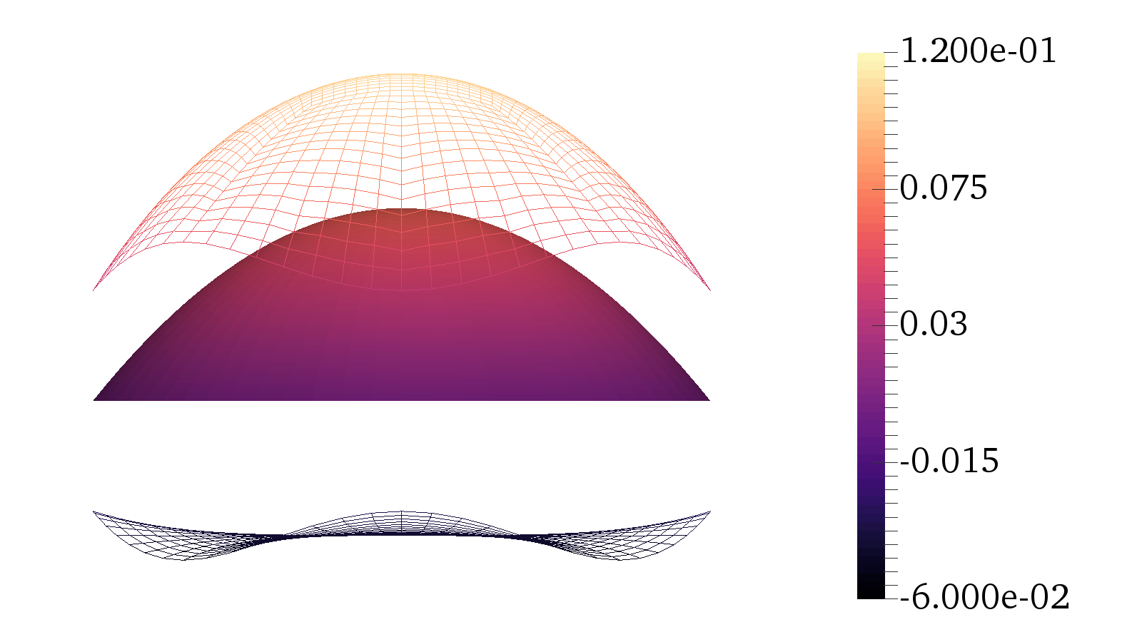
(b) FE solution (top wireframe), IE solution (bottom wireframe), and total solution (solid) with right hand side (14).

Figure 6: Solution domains and sample solution for an interior embedded mesh calculation.

Table 1 reports the self-convergence error in the finite element and integral equation portions of the solution for each test case compared to a fine-grid solution whose parameters are given. We see that the method exhibits the expected order of accuracy given the smoothness of the data. In particular, the method is high-order even near the embedded boundary, in contrast with standard immersed boundary methods. The degree of the FE polynomials space $p$ and the truncation order $p_{\text{QBX}}$ in Quadrature by Expansion are chosen so as to yield equivalent orders of accuracy in the solution–for instance $p=1$ and $p_{\text{QBX}}=2$ yield second-order accurate approximations [37, 38]. In the lower-smoothness test cases, we note a marked difference between the error in the $\infty$- and the 2-norm of the error, both shown. Also, for linear basis functions, the finite element convergence rate in $\|\cdot\|_{\infty;\Omega}$ is suboptimal. This matches analytical expectations as known error estimates of the error in this norm for this basis include a factor of $\log(1/h)$ [39, 40].

Table 1: Self-convergence to a fine mesh solution $u_{\text{ref}}$ vs. smoothness of the right-hand side for the interior problems of Section 2.4. EOC refers to the empirical order of convergence.

Case			Error / Convergence
RHS func.	$p$	$p_{\text{QBX}}$	$h_{\text{fe}}$, $h_{\text{ie}}$	$\|u-u_{\text{ref}}\|_{\infty;\Omega}$	EOC	$\|u-u_{\text{ref}}\|_{2;\Omega}$	EOC
	1	2	0.04, 0.105	4.564$\times 10^{-4}$	–	9.576$\times 10^{-5}$	–
			0.02, 0.052	9.333$\times 10^{-5}$	2.3	1.975$\times 10^{-5}$	2.3
			0.01, 0.026	1.812$\times 10^{-5}$	2.4	3.982$\times 10^{-6}$	2.3
$f_{\text{c}}$	2	3	0.04, 0.105	9.383$\times 10^{-5}$	–	2.189$\times 10^{-5}$	–
			0.02, 0.052	1.032$\times 10^{-5}$	3.2	2.414$\times 10^{-6}$	3.2
			0.01, 0.026	8.840$\times 10^{-7}$	3.5	2.052$\times 10^{-7}$	3.6
	3	4	0.04, 0.105	2.405$\times 10^{-5}$	–	6.072$\times 10^{-6}$	–
			0.02, 0.052	1.510$\times 10^{-6}$	4.9	3.727$\times 10^{-7}$	4.0
			0.01, 0.026	6.887$\times 10^{-8}$	4.5	1.672$\times 10^{-8}$	4.5
	1	2	0.04, 0.105	1.091$\times 10^{-4}$	–	3.040$\times 10^{-5}$	–
			0.02, 0.052	2.110$\times 10^{-5}$	2.4	6.377$\times 10^{-6}$	2.3
			0.01, 0.026	4.201$\times 10^{-6}$	2.3	1.555$\times 10^{-6}$	2.0
$f_{\text{bl}}$	2	3	0.04, 0.105	2.294$\times 10^{-5}$	–	5.736$\times 10^{-6}$	–
			0.02, 0.052	2.453$\times 10^{-6}$	3.2	6.375$\times 10^{-7}$	3.2
			0.01, 0.026	2.219$\times 10^{-7}$	3.5	5.424$\times 10^{-8}$	3.6
	3	4	0.04, 0.105	5.594$\times 10^{-6}$	–	1.597$\times 10^{-6}$	–
			0.02, 0.052	4.103$\times 10^{-7}$	3.8	9.799$\times 10^{-8}$	4.0
			0.01, 0.026	2.396$\times 10^{-8}$	4.1	4.417$\times 10^{-9}$	4.5
	1	2	0.04, 0.105	4.918$\times 10^{-4}$	–	1.008$\times 10^{-4}$	–
			0.02, 0.052	1.882$\times 10^{-4}$	1.4	2.475$\times 10^{-5}$	2.0
			0.01, 0.026	5.620$\times 10^{-5}$	1.7	4.222$\times 10^{-6}$	2.6
$f_{\text{pw}}$	2	3	0.04, 0.105	2.811$\times 10^{-4}$	–	2.417$\times 10^{-5}$	–
			0.02, 0.052	9.098$\times 10^{-5}$	1.6	3.583$\times 10^{-6}$	2.8
			0.01, 0.026	2.489$\times 10^{-5}$	1.9	4.847$\times 10^{-7}$	2.9
	3	4	0.04, 0.105	1.775$\times 10^{-4}$	–	9.453$\times 10^{-6}$	–
			0.02, 0.052	4.730$\times 10^{-5}$	1.9	1.294$\times 10^{-6}$	2.9
			0.01, 0.026	1.219$\times 10^{-5}$	2.0	1.594$\times 10^{-7}$	3.0
— all —	4	5	0.005, 0.013	— reference solution parameters —

3 FE-IE for domains with exclusions

As the next step toward solving the interface problem (1), we extend our FE-IE method to a domain with an exclusion as shown in Figure 5. In contrast to the interior Poisson problem, the solution is sought on the intersection of the unbounded domain $\mathbb{R}^{2}\setminus\Omega$ and the bounded domain $\hat{\Omega}$. That is,

$$-\triangle u(x)= \,f(x)\qquad x\in\hat{\Omega}\backslash\Omega,$$

$$u(x)= \,g(x)\qquad x\in\partial\Omega,$$

(17) $$u(x)= \,\hat{g}(x)\qquad x\in\partial\hat{\Omega}.$$

The generalization to other boundary conditions is left to future work.

Our new approach to FE-IE decomposition for this problem is to solve an interior finite element problem on $\hat{\Omega}$ and an exterior integral equation problem on $\Omega$, with the two solutions coupled only through their boundary values. The setup for this problem is illustrated symbolically in Figure 7.

(a) Problem domain $\hat{\Omega}\backslash\Omega$

(b) IE domain $\mathbb{R}^{d}\backslash\Omega$

(c) FE domain $\hat{\Omega}$

Figure 7: Examples of an actual problem domain and the two computational domains for the coupled FE-IE problem of Section 3 on a domain with a circular hole.

In this way, we allow both methods to play to their individual strengths: the finite element solution exists on a regular, bounded mesh with no exclusions, while the layer potential solution handles boundary conditions present on the boundary of an exclusion, $\partial\Omega$, that is potentially geometrically complex.

3.1 FE-IE decomposition

We solve (3) as before by representing

$$u(x)=u_{1}(x)+u_{2}(x)\quad(x\in\hat{\Omega}\setminus\Omega)$$

and posing a system of BVPs for $u_{1}$ and $u_{2}$:

(18) $$\text{[FE]}\quad-\triangle u_{1}(x) =f(x), \quad x\in\hat{\Omega},$$

$$u_{1}(x) =\hat{g}(x)-u_{2}(x), x\in\partial\hat{\Omega},$$

$$\text{[IE]}\quad-\triangle u_{2}(x) =0, x\in\mathbb{R}^{d}\backslash\Omega,$$

$$u_{2}(x) =g(x)-u_{1}(x), x\in\partial\Omega,$$

$$u_{2}(x)-A\log|x| =o(1) x\to\infty\quad(d=2),$$

$$u_{2}(x) =o(1) x\to\infty\quad(d=3),$$

with a given constant $A$. In two dimensions, (18) includes a far-field boundary condition for $u_{2}$ that differs from the standard far-field BC for the exterior Dirichlet problem, $u(x)=O(1)$ as $x\to\infty$ [27]. There are two reasons for this modification. First, the BVP (3) allows solutions containing a logarithmic singularity within $\Omega$. Without permitting logarithmic blow-up at infinity, such solutions would be ruled out by the splitting (18). Neither $u_{1}$ (nonsingular throughout $\Omega$) nor $u_{2}$ would be able to represent them. Second, allowing nonzero additive constants in $u_{2}$ would lead to a non-uniqueness, since for any given constant $C$, $(u_{1}^{\text{new}},u_{2}^{\text{new}})=(u_{1}+C,u_{2}-C)$ would likewise be an admissible solution.

Next, we support the existence of a solution of the coupled BVPs (18) with the stricter-than-conventional decay condition $o(1)$, we let $A=0$ without loss of generality. We remind the reader that any solution of the exterior Dirichlet problem in two dimensions may be represented as $\mathcal{D}\gamma+C$, for some constant $C$ [27, Thm. 6.25]. Since $(\mathcal{D}\gamma)(x)=O(|x|^{-1})$ ($x\to\infty$) [27, (6.19)], the only loss from our more restrictive decay condition is a constant, which, as discussed above, may be contributed by $u_{1}$.

From (18), we see that the two subproblems are now fully coupled. We cast the subproblem for $u_{1}$ in variational form in anticipation of FEM discretization and the subproblem for $u_{2}$ in terms of layer potentials. To arrive at the coupled system, we first define the operator $\mathcal{R}$ as the restriction to the boundary $\partial\Omega$ and $\hat{\mathcal{R}}$ as the restriction to the boundary $\partial\hat{\Omega}$.

We write $u_{2}$ in terms of an unknown density $\gamma$ using a layer potential operator $\mathcal{A}$ such that $u_{2}=\mathcal{A}\gamma$, while ensuring that the resulting integral equation is of the second kind:

(19) $$\left\{CI+\bar{\mathcal{A}}\right\}\gamma=g-\mathcal{R}u_{1},$$

for some constant $C$.

Next, we decompose $u_{1}$ as

(20) $$u_{1}=\tilde{u}_{1}+\hat{u}_{1}=\tilde{u}_{1}+\mathcal{E}\hat{r}_{1},$$

where $\tilde{u}_{1}\in H^{1}_{0}(\hat{\Omega})$ is zero on the boundary $\partial\hat{\Omega}$ and $\hat{u}_{1}\in H^{1}(\hat{\Omega})$ is used to enforce the boundary conditions. $\hat{u}_{1}$ is defined by a lifting operator $\mathcal{E}:H^{1/2}(\partial\hat{\Omega})\rightarrow H^{1}(\hat{\Omega})$ that selects a specific $\hat{u}_{1}$ in the volume from its boundary restriction $\hat{r}_{1}\equiv\hat{\mathcal{R}}\hat{u}_{1}$. (The precise choice of the lifting operator within these guidelines has no influence on the obtained solution $\hat{u}_{1}$.)

The coupled problem is then to find $\gamma\in C(\partial\Omega)$, $\tilde{u}_{1}\in H^{1}_{0}(\hat{\Omega})$, and $\hat{r}_{1}\in H^{1/2}(\partial\hat{\Omega})$ such that

(21) $$\left[\begin{array}[]{ccc}\ CI+\bar{\mathcal{A}}&\mathcal{R}&\mathcal{R}\mathcal{E}\\ 0&\mathcal{F}(v)&\mathcal{F}(v)\mathcal{E}\\ \hat{\mathcal{R}}\mathcal{A}&0&I\end{array}\right]\left[\begin{array}[]{c}\gamma\\ \tilde{u}_{1}\\ \hat{r}_{1}\end{array}\right]=\left[\begin{array}[]{c}g\\ \mathcal{M}(v)\,f\\ \hat{g}\end{array}\right]\qquad\forall v\in H^{1}_{0}(\hat{\Omega}),$$

where $\mathcal{A}\gamma$ for $u_{2}$ is used in (18).

Next, we isolate the density equation in (21) using a Schur complement, which results in

(22) $$\left\{CI+\bar{\mathcal{A}}-\mathcal{R}\mathcal{U}\left[\begin{array}[]{c}0\\ \hat{\mathcal{R}}\mathcal{A}\end{array}\right]\right\}\gamma=g-\mathcal{R}\mathcal{U}\left[\begin{array}[]{c}f\\ \hat{g}\end{array}\right],$$

with the solution operator $\mathcal{U}:L^{2}(\hat{\Omega})\times H^{1/2}(\partial\hat{\Omega})\rightarrow H^{1}(\hat{\Omega})$, where $\mathcal{U}\,[\zeta;\;\hat{\rho}]$ is defined as the function $\mu=\tilde{\mu}+\mathcal{E}\hat{\rho}$, and where $\tilde{\mu}\in H^{1}_{0}(\hat{\Omega})$ satisfies

(23) $$\mathcal{F}(v)(\tilde{\mu}+\mathcal{E}\hat{\rho})=\mathcal{M}(v)\zeta,\quad v\in H^{1}_{0}(\hat{\Omega}).$$

This allows us to express the IE solution to the coupled problem (21) in terms of input data $f$, $g$, and $\hat{g}$, along with the action of $\mathcal{U}$. Once $\gamma$ is known, the FE solution is found as $u_{1}=\mathcal{U}\,[f;\;\hat{g}-\hat{\mathcal{R}}\mathcal{A}\gamma]$.

The form in (22) identifies two remaining issues. The first is the choice of $C$, which is determined by selecting a layer potential representation $\mathcal{A}$ of $u_{2}$. The conventional choice, a double layer potential, is not suitable because the exterior limit of the double layer operator $\mathcal{D}$ has a nullspace spanned by the constants. A common way of addressing this issue involves adding a layer potential with a lower-order singularity [27]; however, this is inadequate for our coupled FE-IE system (for $d=2$), as we explain below. Instead, we choose $\mathcal{A}=\mathcal{D}+\mathcal{S}$, the sum of the double and single layer potentials, each with the same density. This choice, by the exterior jump relations for the single and double layer potentials [27] establishes $C=1/2$.

Second, uniqueness and existence for (21) hinges on joint compactness of the composition of operators $\mathcal{R}\mathcal{U}\,[0;\;\hat{\mathcal{R}}\mathcal{A}]$ using the next lemma.

Lemma 2.

Let $\hat{\Omega}\subseteq\mathbb{R}^{n}$ ($n=2,3$) be bounded, satisfy an exterior sphere condition at every boundary point, and contain a domain $\Omega$ with a $C^{\infty}$ boundary. Further assume that $d(\partial\hat{\Omega},\partial\Omega)>0$. Then the operator $\mathcal{R}\mathcal{U}\,[0;\;\hat{\mathcal{R}}\mathcal{A}]:C(\partial\Omega)\rightarrow C(\partial\Omega)$ is compact.

Proof.

First consider the operator $\hat{\mathcal{R}}\mathcal{A}$. Let $\gamma\in C(\partial\Omega)$. $\hat{\mathcal{R}}\mathcal{A}\gamma$ evaluates the layer potential on the outer boundary $\partial\hat{\Omega}$. Since $x\mapsto\mathcal{A}\gamma(x)$ is harmonic, $\mathcal{A}\gamma(x)$ is analytic for $x\not\in\partial\Omega$ [27, Thm. 6.6], and the restriction to the boundary $\partial\hat{\Omega}$, $\hat{\mathcal{R}}\mathcal{A}\gamma$, is at least continuous.

Next, consider the composite operator $\gamma\mapsto\mathcal{U}\,[0;\;\hat{\mathcal{R}}\mathcal{A}\gamma]$. The boundary value problem

(24) $$\quad-\triangle w(x) =0, \quad x\in\hat{\Omega},$$

$$w(x) =\hat{\mathcal{R}}\mathcal{A}\gamma(x), x\in\partial\hat{\Omega}$$

has a classical solution $w\in C^{0}(\overline{\hat{\Omega}})\cap C^{2}(\hat{\Omega})$ [41, Thm. 6.13] because of the regularity of the domain and data. More precisely, even $w\in C^{\infty}(\hat{\Omega})$ by [41, Thm. 6.17].

The classical solution $w$ found above is identical to the unique ([41, Cor. 8.2]) variational solution $\mathcal{U}\,[0;\;\hat{\mathcal{R}}\mathcal{A}\gamma]\in H^{1}(\hat{\Omega})$. The classical maximum principle (e.g. [41, Thm. 3.1]) then yields that

$$\|\mathcal{R}\mathcal{U}\,[0;\;\hat{\mathcal{R}}\mathcal{A}\gamma]\|_{\infty}\leq\|\hat{\mathcal{R}}\mathcal{A}\gamma\|_{\infty}.$$

Consequently, we have that $\mathcal{R}\mathcal{U}$ is bounded and $\hat{\mathcal{R}}\mathcal{A}$ is compact. The composition of a compact operator with a bounded operator is compact, which completes the proof. ∎

Using slightly different machinery, a discrete version of Lemma 2 is available at least in $\mathbb{R}^{2}$. To this end, let $\hat{\Omega}\subset\mathbb{R}^{2}$ be convex and polygonal and define a finite element subspace $V^{h}\subset H^{1}(\hat{\Omega})$ of continuous polynomials of degree $\geq 1$ on a quasi-uniform triangulation of $\hat{\Omega}$ (in the sense of [40]). Also define $V^{h}_{0}:=H^{1}_{0}(\hat{\Omega})\cap V^{h}$. Further define the discrete lifting operator $\mathcal{E}^{h}:H^{1/2}(\partial\hat{\Omega})\to V^{h}$ and the discrete solution operator $\mathcal{U}^{h}:V^{h}\times H^{1/2}(\partial\hat{\Omega})\to V^{h}$ where $\mathcal{U}^{h}\,[\zeta;\;\hat{\rho}]$ is defined as the function $\tilde{\mu}^{h}+\mathcal{E}^{h}\hat{\rho}$, where $\tilde{\mu}^{h}\in V^{h}_{0}$ satisfies

$$\mathcal{F}(v^{h})(\tilde{\mu}^{h}+\mathcal{E}^{h}\hat{\rho})=\mathcal{M}(v^{h})\zeta,\quad v^{h}\in V^{h}_{0}.$$

(Again, the precise choice of the discrete lifting operator within these guidelines has no influence on the obtained solution.)

Theorem 1.

Assume that $\hat{\Omega}\subset\mathbb{R}^{2}$ is bounded, convex, and polygonal and contains a domain $\Omega$ with a $C^{\infty}$ boundary. Further assume that $d(\partial\hat{\Omega},\partial\Omega)>\epsilon$ for some finite $\epsilon>0$. Let the family of operators

$${\{\hat{\mathcal{R}}\mathcal{A}^{h}:C(\partial\Omega)\rightarrow C(\partial\hat{\Omega})\}}_{h}$$

be collectively compact and the functions in their ranges be harmonic. Then the family of operators

$${\{\gamma\mapsto\mathcal{R}\mathcal{U}^{h}\,[0;\;\hat{\mathcal{R}}\mathcal{A}^{h}\gamma]:C(\partial\Omega)\rightarrow C(\partial\Omega)\}}_{h}$$

is collectively compact for sufficiently small $h$.

Proof.

First consider the operator $\hat{\mathcal{R}}\mathcal{A}^{h}$. Let $\gamma\in C(\partial\Omega)$. $\hat{\mathcal{R}}\mathcal{A}^{h}\gamma$ evaluates the layer potential on the outer boundary $\partial\hat{\Omega}$. Since $x\mapsto\mathcal{A}^{h}\gamma(x)$ is harmonic, it is also analytic for $x\not\in\partial\Omega$ [27, Thm. 6.6], and so is its restriction $\hat{\mathcal{R}}\mathcal{A}^{h}\gamma$ to the boundary $\partial\hat{\Omega}$ is at least continuous.

The discrete maximum principle [40] yields that

(25) $$\|\mathcal{R}\mathcal{U}^{h}\,[0;\;\hat{\mathcal{R}}\mathcal{A}^{h}\gamma]\|_{\infty}\leq C\|\hat{\mathcal{R}}\mathcal{A}^{h}\gamma\|_{\infty}.$$

where $C$ is independent of $h$. Noting $\mathcal{R}\mathcal{U}^{h}\,[0;\;\hat{\mathcal{R}}\mathcal{A}^{h}\gamma]\in V_{h}\subset C(\hat{\Omega})$ by construction, we have that $\mathcal{R}\mathcal{U}^{h}\,[0;\;\hat{\mathcal{R}}\mathcal{A}^{h}]:C(\partial\Omega)\rightarrow C(\partial\Omega)$, with bounded $\mathcal{R}\mathcal{U}^{h}$ and compact $\hat{\mathcal{R}}\mathcal{A}^{h}$. We obtain our claim since the composition of a compact operator with a bounded operator is compact, noting that collective compactness follows from the $h$-independence of the constant in (25). ∎

The form of the operator in (22) is

(26) $$\mathcal{Z}=CI+\bar{\mathcal{A}}-\mathcal{R}\mathcal{U}\,[0;\;\hat{\mathcal{R}}\mathcal{A}].$$

Thus, Lemma 2 and Theorem 1 establish that the integral equation (22) is of the second kind and its discretization takes a form to which Anselone’s Theorem applies. The operator $\mathcal{Z}$ in (26) and its discrete version are the sum of an identity and a compact operator. Consequently, by the Fredholm alternative, if the operator has no nullspace, then existence of the solution is guaranteed. Again, convergence of the solution as $h\to 0$ is assured by Anselone’s theorem.

We highlight some factors that influenced our choice of the IE representation. The purely IE part of the operator, $CI+\bar{\mathcal{A}}$, represents the behavior on $\partial\Omega$ of a harmonic function exterior to $\partial\Omega$, while the coupled FE part, $\mathcal{R}\mathcal{U}\,[0;\;\hat{\mathcal{R}}]\mathcal{A}$, is approximating a harmonic function interior to $\partial\hat{\Omega}$; both functions have the same value on the boundary $\partial\hat{\Omega}$ (but not on $\partial\Omega$). A nontrivial nullspace exists in (22) if the intersection of the ranges of the operators is nontrivial. Distinct decay behavior of interior and exterior Dirichlet solutions generally keeps the ranges of these operators from having a nontrivial intersection.

3.1.1 Remarks on the Behavior of the Error

The observed convergence behavior is similar to that of the interior case, but with additional components stemming from the FE error and the IE representation error in the operator $\mathcal{R}\mathcal{U}\,[0;\;\hat{\mathcal{R}}\mathcal{A}]$. As it is a composition of operators with known high-order accuracy, however, the composite scheme has the same asymptotic error behavior as the less accurate of its constituent parts, analogous to Lemma 1. In particular, the error in the $\mathcal{U}\,[0;\;\hat{\mathcal{R}}\mathcal{A}]$ part of the overall operator on $\gamma$ is bounded by the error in its boundary conditions—the operator error on $\hat{\mathcal{R}}\mathcal{A}$—by the weak discrete maximum principle. Thus the leading term effect of the composition of the two is the same as the other FE or IE operator error terms, depending on which error is larger.

The error behavior of the finite element solution $u_{1}$ once again follows standard finite element convergence theory, with additional error incurred through error in $\hat{\mathcal{R}}\mathcal{A}\gamma$ in the boundary condition. However, again the additional FE error is bounded by the error in $\hat{\mathcal{R}}\mathcal{A}\gamma$ through the discrete weak maximum principle. The net result is that we expect to retain the same overall order of convergence as in the interior case and with similar dependence on the FE and IE solvers.

3.2 Numerical experiments

We consider the coupled system (21) with the exact solution

$$u=\log(r_{0})+2\sin(\pi x)\sin(\pi y),$$

where

$$r_{0}=\sqrt{(x-0.1)^{2}+(y+0.02)^{2}}.$$

In each numerical example, GMRES is used to solve the linear system with algebraic multigrid preconditioning in the case of the FE operators.

The IE, FE, and coupled solutions are shown for a starfish exclusion in Figure 9 and where the parametrization is given by

(27) $$\gamma(t)=\begin{bmatrix}1/2+(1/8)\sin{(10\pi t)}\cos{(2\pi t)},\\ 1/2+(1/8)\sin{(10\pi t)}\sin{(2\pi t)},\end{bmatrix}\quad t\in[0,1].$$

Figure 8 gives a visual impression of the obtained solution. Convergence results are found in Table 2.

As expected, we observe high-order convergence.

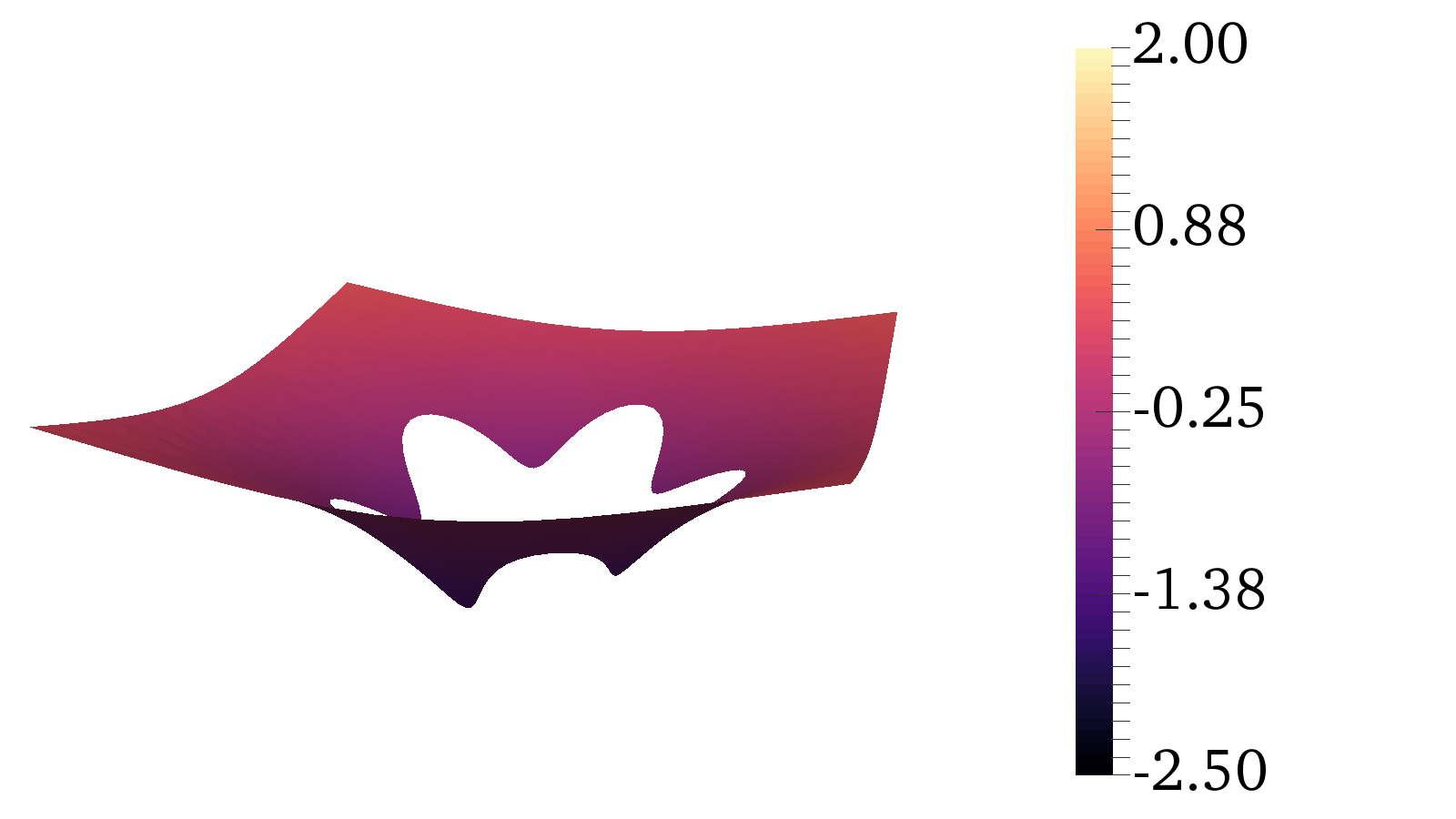
(a) IE solution.

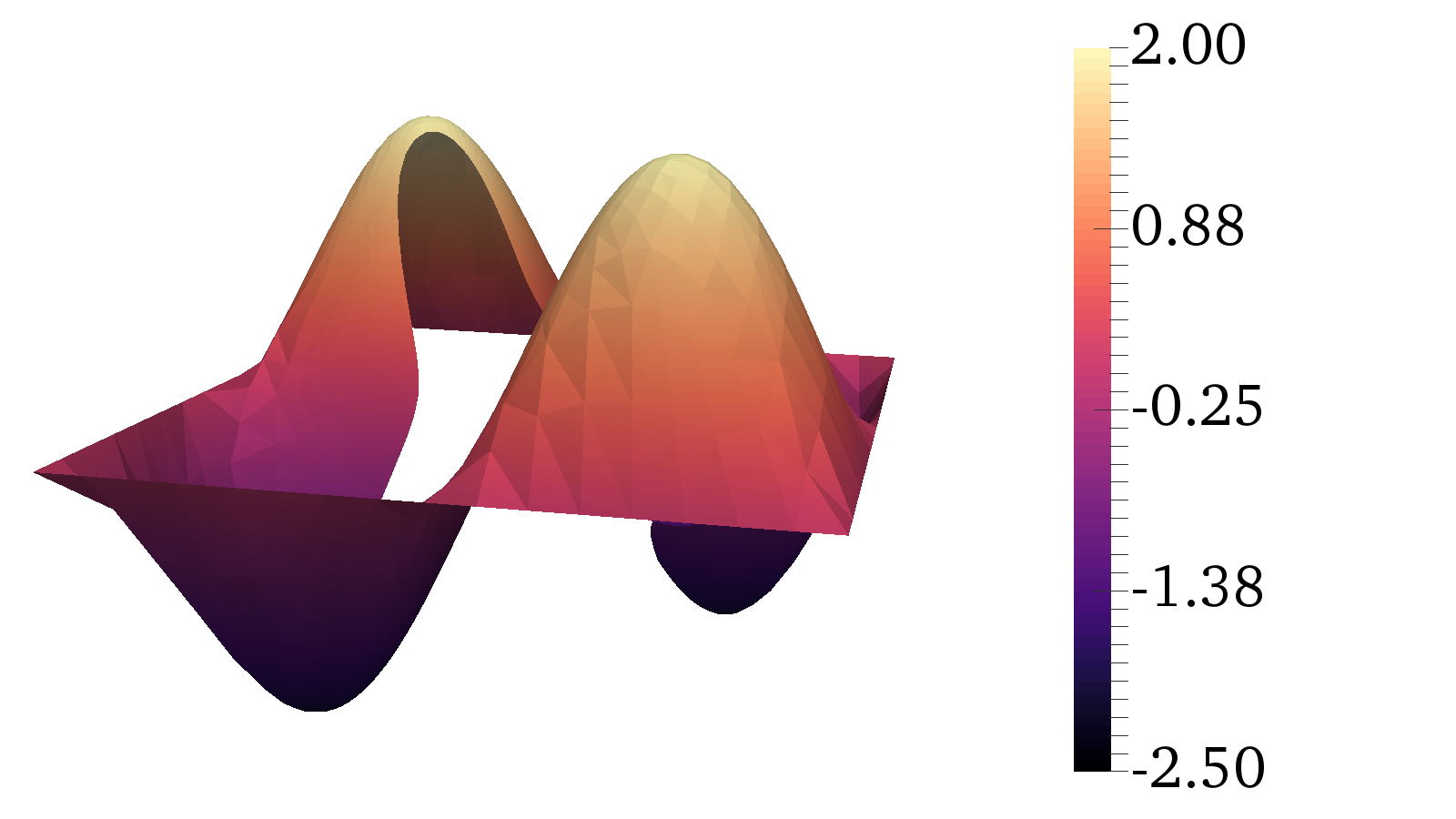
(b) FE solution.

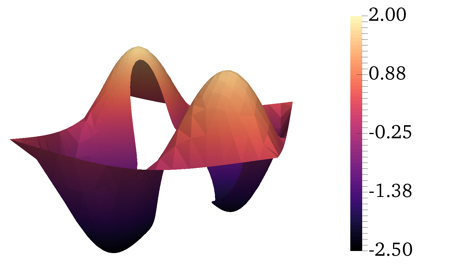
(c) Total solution.

Figure 8: Individual and combined solutions on the true domain for the exterior embedded mesh problem.

Figure 9: Starfish domain excluded from $\hat{\Omega}=[-1,-1]\times[-1,1]$

Table 2: Convergence of coupled interior-exterior FE-IE system for the excluded starfish domain.

$p$	$p_{\text{QBX}}$	$h_{\text{fe}}$, $h_{\text{ie}}$	$\left\|\text{error}\right\|_{\infty;\hat{\Omega}\backslash\Omega}$	order	$\|\text{error}\|_{L^{2}(\hat{\Omega}\backslash\Omega)}$	order
1	2	0.133, 0.327	5.80$\times 10^{-2}$	–	2.38$\times 10^{-2}$	–
		0.067, 0.170	1.28$\times 10^{-2}$	2.2	6.08$\times 10^{-3}$	2.0
		0.033, 0.085	3.47$\times 10^{-3}$	1.9	1.47$\times 10^{-3}$	2.0
		0.017, 0.043	8.46$\times 10^{-4}$	2.0	3.74$\times 10^{-4}$	2.0
2	3	0.133, 0.327	1.21$\times 10^{-2}$	–	2.05$\times 10^{-3}$	–
		0.067, 0.170	2.82$\times 10^{-3}$	2.1	3.29$\times 10^{-4}$	2.6
		0.033, 0.085	5.53$\times 10^{-4}$	2.3	3.70$\times 10^{-5}$	3.2
		0.017, 0.043	6.48$\times 10^{-5}$	3.1	3.65$\times 10^{-6}$	3.3
3	4	0.133, 0.327	1.00$\times 10^{-2}$	–	1.12$\times 10^{-3}$	–
		0.067, 0.170	1.73$\times 10^{-3}$	2.5	9.97$\times 10^{-5}$	3.5
		0.033, 0.085	1.91$\times 10^{-4}$	3.2	7.19$\times 10^{-6}$	3.8
		0.017, 0.043	1.47$\times 10^{-5}$	3.7	4.08$\times 10^{-7}$	4.1

4 FE-IE for Interface Problems

In this section, we combine the elements described in Sections 2 and 3 to form a new embedded boundary method for the interface problem (1). In our approach, a fictitious domain $\hat{\Omega}^{i}$ is introduced so that $\Omega^{i}\subset\hat{\Omega}^{i}$, defining $\hat{\Omega}^{e}$ as $\Omega^{e}\cup\Omega^{i}$. Then the problem is separated into two subproblems with an appropriate FE-IE splitting on each. This is illustrated in Figure 10.

Figure 10: Coupled subproblems for an embedded interface.

There are four components to the combined solution: $u_{1}^{i}:\hat{\Omega}^{i}\to\mathbb{R}$ and $u_{2}^{i}:\Omega^{i}\to\mathbb{R}$ for the interior solution, plus $u_{1}^{e}:\hat{\Omega}^{e}\to\mathbb{R}$ and $u_{2}^{e}:\mathbb{R}^{d}\backslash\Omega^{i}\to\mathbb{R}$ for the exterior solution.

As before, $u_{1}^{i}$ and $u_{1}^{e}$ represent the finite element components of the solution. For the interior and exterior integral equation solutions, we choose the combined representation

$$u_{2}^{i}=\alpha_{1}\mathcal{D}\gamma^{i}+\alpha_{2}\mathcal{S}\gamma^{e},\quad\text{and}\quad u_{2}^{e}=\alpha_{3}\mathcal{D}\gamma^{i}+\alpha_{4}\mathcal{S}\gamma^{e},$$

for some constant coefficients $\alpha_{j}$. We next determine $\alpha_{j}$ to ensure that all integral operators are of the second kind.

Taking the limits of these expressions at the interface and adding the interface restrictions of the finite element solutions gives the following form for the interface conditions:

(28) $$\mathcal{R}u_{1}^{i}+\alpha_{1}\left(\mathcal{D}_{-}\right)\gamma^{i}+\alpha_{2}\left(\mathcal{S}_{-}\right)\gamma^{e}=c(\mathcal{R}\partial_{n})u_{1}^{e}+c\alpha_{3}\left(\mathcal{D}_{+}\right)\gamma^{i}+c\alpha_{4}\left(\mathcal{S}_{+}\right)\gamma^{e}+a(x),$$

and

(29) $$(\mathcal{R}\partial_{n})u_{1}^{i}+\alpha_{1}\partial_{n}\left(\mathcal{D}_{-}\right)\gamma^{i}+\alpha_{2}\partial_{n}\left(\mathcal{S}_{-}\right)\gamma^{e}=\kappa(\mathcal{R}\partial_{n})u_{1}^{e}+\kappa\alpha_{3}\partial_{n}\left(\mathcal{D}_{+}\right)\gamma^{i}+\kappa\alpha_{4}\partial_{n}\left(\mathcal{S}_{+}\right)\gamma^{e}+b(x),$$

where $\mathcal{D}_{\pm}$ indicates the interior ($-$) or exterior ($+$) limit of the double-layer operator; similarly for $\mathcal{S}_{\pm}$. The $(\mathcal{R}\partial_{n})$ operator is defined analogous to $\mathcal{R}$, but for gradient of the FE solution normal to the interface $\Gamma$.

We use the well-known jump conditions for layer potentials [27] and collect the terms on each operator, which yields

(30) $$\mathcal{R}u_{1}^{i}+\left[-\frac{\alpha_{1}+c\alpha_{3}}{2}I+(\alpha_{1}-c\alpha_{3})\bar{\mathcal{D}}\right]\gamma^{i}=c\mathcal{R}u_{1}^{e}+\left[-\alpha_{2}+c\alpha_{4}\right]\bar{\mathcal{S}}\gamma^{e}+a(x)$$

and

(31) $$(\mathcal{R}\partial_{n})u_{1}^{i}+\left[\frac{\alpha_{2}+\kappa\alpha_{4}}{2}I+(\alpha_{2}-\kappa\alpha_{4})\bar{\mathcal{S}}^{\prime}\right]\gamma^{e}=\kappa(\mathcal{R}\partial_{n})u_{1}^{e}+\left[-\alpha_{1}+\kappa\alpha_{3}\right]\bar{\mathcal{D}}^{\prime}\gamma^{i}+b(x).$$

To determine suitable values for $\alpha_{j}$, first we eliminate the hypersingular operator $\bar{\mathcal{D}}^{\prime}$ from (31), necessitating

(32) $$\alpha_{1}=\kappa\alpha_{3}.$$

With $\bar{\mathcal{D}}^{\prime}$ eliminated, (31) is an equation for $\gamma^{e}$ with operator

$$\frac{\alpha_{2}+\kappa\alpha_{4}}{2}I+(\alpha_{2}-\kappa\alpha_{4})\bar{\mathcal{S}}^{\prime}.$$

In order to have an operator with only the trivial nullspace, guaranteeing a unique solution for $\gamma^{e}$, we select the coefficients of $I$ and $\bar{\mathcal{S}}^{\prime}$ to have opposite sign.

Next consider the jump condition (30). Enforcing the requirement (32), the operator on $\gamma^{i}$ is

(33) $$-\frac{(\kappa+c)\alpha_{3}}{2}I+(\kappa-c)\alpha_{3}\bar{\mathcal{D}}.$$

This results in three possibilities based on $\kappa$ and $c$:

1. $\kappa\neq c$ and $\kappa\neq-c$, where both terms remain,

2. $\kappa=c$, where the double-layer term drops out, and

3. $\kappa=-c$, where the identity term is eliminated.

We consider each case in the following sections.

4.1 The case $\kappa\neq c$ and $\kappa\neq-c$

Combining the interface condition equations (30) and (31) with the condition (32) and the interior and exterior FE problems for $u_{1}^{i}$ and $u_{1}^{e}$ yields a coupled system for the interface problem: with $\mathcal{F}^{i}(v)$ and $v\in H^{1}_{0}(\hat{\Omega}^{i})$ for the interior problem and $\mathcal{F}^{e}(w)$ and $w\in H^{1}_{0}(\hat{\Omega}^{e})$ for the coupled exterior problem, we seek $(\gamma^{i},\gamma^{e})\in C(\Gamma)$, $u_{1}^{i}\in H_{0}^{1}(\hat{\Omega}^{i})$, $\tilde{u}_{1}^{e}\in H_{0}^{1}(\hat{\Omega}^{e})$, and $\hat{r}_{1}\in H^{1/2}(\partial\hat{\Omega}^{e})$ such that

(34) $$\mathcal{C}\left[\begin{array}[]{c}\gamma^{i}\\ \gamma^{e}\\ \hline\cr u_{1}^{i}\\ \tilde{u}_{1}^{e}\\ \hat{r}_{1}^{e}\end{array}\right]=\left[\begin{array}[]{c}a(x)\\ b(x)\\ \hline\cr\mathcal{M}^{i}(v)\,f^{i}\\ \mathcal{M}^{e}(w)\,f^{e}\\ \hat{g}\end{array}\right]\qquad\textnormal{for all $v\in H^{1}_{0}(\hat{\Omega}^{i}),w\in H_{0}^{1}(\hat{\Omega}^{e})$,}$$

where

(35) $$\mathcal{C}=\left[\begin{array}[]{c c | c c c}-\frac{1}{2}(\kappa+c)\alpha_{3}I+(\kappa-c)\alpha_{3}\bar{\mathcal{D}}&(\alpha_{2}-c\alpha_{4})\bar{\mathcal{S}}&\mathcal{R}&-c\mathcal{R}&-c\mathcal{R}\mathcal{E}^{e}\\ 0&\frac{1}{2}(\alpha_{2}+\kappa\alpha_{4})I+(\alpha_{2}-\kappa\alpha_{4})\bar{\mathcal{S}}^{\prime}&(\mathcal{R}\partial_{n})&-\kappa(\mathcal{R}\partial_{n})&\kappa(\mathcal{R}\partial_{n})\mathcal{E}^{e}\\ \hline\cr 0&0&\mathcal{F}^{i}(v)&0&0\\ 0&0&0&\mathcal{F}^{e}(w)&\mathcal{F}^{e}(w)\mathcal{E}^{e}\\ \alpha_{3}\hat{\mathcal{R}}^{e}\mathcal{D}&\alpha_{4}\hat{\mathcal{R}}^{e}\mathcal{S}&0&0&I\\ \end{array}\right].$$

The lifting operator $\mathcal{E}^{e}$ is as described in Section 3.1 and acts on the boundary $\partial\hat{\Omega}^{e}$. The source functions $f^{i}:\hat{\Omega}^{i}\to\mathbb{R}$ and $f^{e}:\hat{\Omega}^{e}\to\mathbb{R}$ are once again suitably restricted and/or extended versions of the right-hand side $f$. From this we see that $a(x)$ and $b(x)$ in the jump conditions are handled as additional terms on the right-hand side of the system.

4.1.1 A Solution Procedure Involving the Schur Complement

For the exterior problem, we apply a Schur complement to (34). To simplify notation, we apply (32) and define the block IE operator as

$$\underline{\underline{\mathcal{I}}}+\underline{\underline{\bar{\mathcal{A}}}}=\begin{bmatrix}-\frac{1}{2}(\kappa+c)\alpha_{3}I+(\kappa-c)\alpha_{3}\bar{\mathcal{D}}&(\alpha_{2}-c\alpha_{4})\bar{\mathcal{S}}\\ 0&\frac{1}{2}(\alpha_{2}+\kappa\alpha_{4})I+(\alpha_{2}-\kappa\alpha_{4})\bar{\mathcal{S}}^{\prime}\end{bmatrix}.$$

We also define the block coupling operator

$$\underline{\underline{\mathcal{R}}}=\begin{bmatrix}\mathcal{R}&-c\mathcal{R}\\ (\mathcal{R}\partial_{n})&-\kappa(\mathcal{R}\partial_{n})\end{bmatrix}.$$

As restriction to the outer boundary $\partial\hat{\Omega}^{e}$ is only necessary for $u_{2}^{e}$, we do not need a block form of $\hat{\mathcal{R}}$. Rather,

$$\hat{\mathcal{R}}^{e}\mathcal{A}^{e}=\begin{bmatrix}\alpha_{3}\hat{\mathcal{R}}^{e}\mathcal{D}&\alpha_{4}\hat{\mathcal{R}}^{e}\mathcal{S}\end{bmatrix}$$

will suffice.

Finally, we define the block FE solution operator $\underline{\underline{\mathcal{U}}}:L^{2}(\hat{\Omega}^{i})\times L^{2}(\hat{\Omega}^{e})\times H^{1/2}(\partial\hat{\Omega}^{e})\rightarrow H_{0}^{1}(\hat{\Omega}^{i})\times H^{1}(\hat{\Omega}^{e})$ such that the $\mu^{i}\in H_{0}^{1}(\hat{\Omega}^{i})$ and $\tilde{\mu}^{e}\in H^{1}_{0}(\hat{\Omega}^{e})$ defined by $[\mu^{i};\;\tilde{\mu}^{e}+\mathcal{E}^{e}\hat{\rho}]=\underline{\underline{\mathcal{U}}}\,[\zeta^{i};\,\zeta^{e};\,\hat{\rho}]$ satisfy

(36) $$\mathcal{F}^{i}(v)\mu^{i} =\mathcal{M}^{i}(v)\zeta^{i} \forall v\in H_{0}^{1}(\hat{\Omega}^{i}),$$

$$\mathcal{F}^{e}(w)(\tilde{\mu}^{e}+\mathcal{E}^{e}\hat{\rho}) =\mathcal{M}^{e}(w)\zeta^{e} \forall w\in H_{0}^{1}(\hat{\Omega}^{e}).$$

We then write the equations for the density functions as

(37) $$\left\{\underline{\underline{\mathcal{I}}}+\underline{\underline{\bar{\mathcal{A}}}}-\underline{\underline{\mathcal{R}}}\,\underline{\underline{\mathcal{U}}}\begin{bmatrix}0\\ 0\\ \hat{\mathcal{R}}^{e}\mathcal{A}^{e}\end{bmatrix}\right\}\left[\begin{array}[]{c}\gamma^{i}\\ \gamma^{e}\end{array}\right]=\left[\begin{array}[]{c}a(x)\\ b(x)\end{array}\right]-\underline{\underline{\mathcal{R}}}\,\underline{\underline{\mathcal{U}}}\begin{bmatrix}f^{i}\\ f^{e}\\ \hat{g}\end{bmatrix}.$$

Once the densities are known, the FE solutions are defined as $\underline{\underline{\mathcal{U}}}\,[f^{i};\,f^{e};\,\hat{g}-\hat{\mathcal{R}}^{e}\mathcal{A}^{e}][\gamma^{i};\;\gamma^{e}]$.

The equation (37) very closely resembles (22) for the exterior case in Section 3. The main difference here—apart from the doubling of the number of variables—is the appearance of $(\mathcal{R}\partial_{n})$ terms in $\underline{\underline{\mathcal{R}}}$ and thus in the operator on $[\gamma^{i};\;\gamma^{e}]$ in (37). As the output from $\hat{\mathcal{R}}^{e}\mathcal{A}^{e}[\gamma^{i};\;\gamma^{e}]$ is smooth, however, the result of $\underline{\underline{\mathcal{U}}}\,[0;\,0;\,\hat{\mathcal{R}}^{e}\mathcal{A}^{e}][\gamma^{i};\;\gamma^{e}]$ is smooth for most domains, as it is approximating a harmonic function for $u_{1}^{e}$ and will return $u_{1}^{i}=0$ due to the homogeneous boundary conditions enforced on $u_{1}^{i}$. We expect this to mitigate any negative effects on the conditioning of the numerical system.

4.2 The case $\kappa=c$

In this case, the $\bar{\mathcal{D}}$ term drops out of the operator on $\gamma^{i}$. We may choose $\alpha_{2}=c\alpha_{4}=\kappa\alpha_{4}$ which results in IE block in the form of a scaled identity:

(38) $$[\kappa=c\text{ case}]\qquad\underline{\underline{\mathcal{I}}}+\underline{\underline{\bar{\mathcal{A}}}}=\begin{bmatrix}-\frac{1}{2}(\kappa+c)\alpha_{3}I&0\\ 0&\kappa\alpha_{2}I\end{bmatrix}.$$

4.3 The case $\kappa=-c$

In this case, the operator on $\gamma^{i}$ as defined in (33) loses the identity term, resulting in an equation for $\gamma^{i}$ which is not of the second kind. We leave this to future work.

4.4 Numerical experiments

We demonstrate the behavior of the method on two test problems, one with $\kappa\neq c$ and one with $\kappa=c$. The choices for the coefficients of the layer potential representation are summarized in Table 3.

Table 3: Choices of coefficients for numerical experiments

Case	$\alpha_{1}$	$\alpha_{2}$	$\alpha_{3}$	$\alpha_{4}$
$\kappa\neq c$:	$\kappa\alpha_{3}$	0	$1/(\kappa-c)$	$1/\kappa$
$\kappa=c$:	$\kappa\alpha_{3}$	1	$-1/\kappa$	$1/\kappa$

4.4.1 The quadratic-log test case

In this manufactured-solution experiment, the interface $\Gamma$ is a circle of radius $0.5$ and $\Omega^{e}\cup\Omega^{i}$ is the square $[-1,-1]\times[-1,1]$. Relevant data for this test case is given in Table 4 with the solution shown in Figure 11. We note that the right-hand side $f$ in this example exhibits a discontinuity, however the reduction in convergence order discussed in Section 1 does not occur because, by way of their given expressions, both may be smoothly extended into the respective other domain.

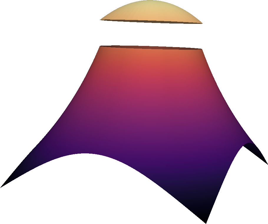
(a) quadratic-log

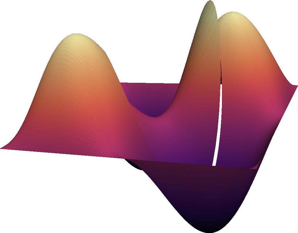
(b) sine-linear

Figure 11: Numerical solutions for the test cases.

case	interior			exterior			interface
	$u$	$f$	$\hat{g}$	$u$	$f$	$\hat{g}$	$\kappa$	$c$	$a(x)$	$b(x)$
quadratic-log	$-\frac{5}{6}r^{2}$	$\frac{10}{3}$	—	$-\frac{5}{4}\log{\left(\frac{1}{2r}\right)}-\frac{11}{24}$	0	$u^{*}$	1/3	1	1/4	0
sine-linear	$s_{x}s_{y}+x+y$	$4\pi^{2}s_{x}s_{y}$	—	$s_{x}s_{y}$	$4\pi^{2}s_{x}s_{y}$	$u^{*}$	1	1	$x+y$	${\bf 1}\cdot\hat{n}$

Table 4: Data for the quadratic-log and sine-linear test cases. $s_{x}$ and $s_{y}$ denote $\sin{(2\pi x)}$ and $\sin{(2\pi y)}$.

Convergence is shown in Table 5. We

achieve high-order convergence for the FE basis functions $p\geq 2$ and attribute the lower convergence order to the fact that the solution now depends on the FE derivative, and as a result we expect to lose an order of convergence in the gradient representation compared to the solution representation.

An interesting artifact arises in the convergence for $p=1$: there is negative convergence between the coarsest and second-coarsest meshes. This is due to the appearance of the derivative of the finite element solution in the system. For $p=1$, the derivative of the FE solution is piecewise constant. On a coarse mesh, piecewise constants poorly represent even smooth solutions with variation. As a result, the $p=1$ case is sensitive to element placement, especially for coarse meshes. Because of this effect we disregard data for $p=1$ and recommend using at least $p=2$.

Table 5: Convergence data for quadratic-log test problem with $\hat{\Omega}^{i}=[-0.6,-0.6]\times[0.6,0.6]$

$p$	$p_{\text{QBX}}$	solution	$h_{\text{fe}}$, $h_{\text{ie}}$	$\|\text{error}\|_{\infty;\Omega}$	order	$\|\text{error}\|_{L^{2}(\Omega)}$	order
1	2	interior	0.080, 0.224	6.93$\times 10^{-3}$	–	3.81$\times 10^{-3}$	–
			0.040, 0.108	1.43$\times 10^{-2}$	-1.0	1.14$\times 10^{-2}$	-1.5
			0.020, 0.053	5.48$\times 10^{-3}$	1.4	3.88$\times 10^{-3}$	1.5
			0.010, 0.026	1.51$\times 10^{-3}$	1.8	8.11$\times 10^{-4}$	2.2
1	2	exterior	0.080, 0.224	8.53$\times 10^{-3}$	–	5.61$\times 10^{-3}$	–
			0.040, 0.108	1.51$\times 10^{-2}$	-0.8	1.05$\times 10^{-2}$	-0.9
			0.020, 0.053	5.34$\times 10^{-3}$	1.5	3.43$\times 10^{-3}$	1.6
			0.010, 0.026	1.48$\times 10^{-3}$	1.8	7.23$\times 10^{-4}$	2.2
2	3	interior	0.080, 0.224	3.64$\times 10^{-3}$	–	2.57$\times 10^{-3}$	–
			0.040, 0.108	6.41$\times 10^{-4}$	2.4	3.88$\times 10^{-4}$	2.6
			0.020, 0.053	7.57$\times 10^{-5}$	3.0	4.34$\times 10^{-5}$	3.1
			0.010, 0.026	1.05$\times 10^{-5}$	2.8	5.64$\times 10^{-6}$	2.9
2	3	exterior	0.080, 0.224	5.14$\times 10^{-3}$	–	2.63$\times 10^{-3}$	–
			0.040, 0.108	7.79$\times 10^{-4}$	2.6	3.78$\times 10^{-4}$	2.7
			0.020, 0.053	8.63$\times 10^{-5}$	3.1	4.15$\times 10^{-5}$	3.1
			0.010, 0.026	1.12$\times 10^{-5}$	2.9	5.27$\times 10^{-6}$	2.9
3	4	interior	0.080, 0.224	7.95$\times 10^{-4}$	–	4.22$\times 10^{-4}$	–
			0.040, 0.108	8.04$\times 10^{-5}$	3.1	3.83$\times 10^{-5}$	3.3
			0.020, 0.053	6.34$\times 10^{-6}$	3.6	2.75$\times 10^{-6}$	3.7
			0.010, 0.026	4.52$\times 10^{-7}$	3.8	1.91$\times 10^{-7}$	3.8
3	4	exterior	0.080, 0.224	1.16$\times 10^{-3}$	–	4.77$\times 10^{-4}$	–
			0.040, 0.108	9.99$\times 10^{-5}$	3.4	3.99$\times 10^{-5}$	3.4
			0.020, 0.053	7.13$\times 10^{-6}$	3.7	2.77$\times 10^{-6}$	3.8
			0.010, 0.026	4.80$\times 10^{-7}$	3.8	1.87$\times 10^{-7}$	3.8

4.4.2 The sine-linear test case

Next, we consider a test case for which $\kappa=c$; its data is summarized in Table 4 and shown for a circular interface in Figure 11(b). This is once again a manufactured solution with the same forcing function $f$ through $\Omega^{i}\cup\Omega^{e}$. The extra linear function added to the interior solution influences the numerical system only through the non-homogeneous jump conditions $a(x)$ and $b(x)$. Convergence data is shown in Table 6 for the starfish interface.

Again, we see high-order convergence.

Table 6: Convergence data for sine-linear test problem with $\Omega^{i}=$ starfish curve (27)

$p$	$p_{\text{QBX}}$	solution	$h_{\text{fe}}$, $h_{\text{ie}}$	$\|\text{error}\|_{\infty;\Omega}$	order	$\|\text{error}\|_{L^{2}(\Omega)}$	order
1	2	interior	0.080, 0.327	7.43$\times 10^{-2}$	–	1.66$\times 10^{-2}$	–
			0.040, 0.170	5.54$\times 10^{-3}$	3.7	1.27$\times 10^{-3}$	3.7
			0.020, 0.085	1.37$\times 10^{-3}$	2.0	3.17$\times 10^{-4}$	2.0
			0.010, 0.043	3.63$\times 10^{-4}$	1.9	7.87$\times 10^{-5}$	2.0
1	2	exterior	0.080, 0.327	7.32$\times 10^{-2}$	–	2.63$\times 10^{-2}$	–
			0.040, 0.170	5.63$\times 10^{-3}$	3.7	3.08$\times 10^{-3}$	3.1
			0.020, 0.085	1.45$\times 10^{-3}$	2.0	7.28$\times 10^{-4}$	2.1
			0.010, 0.043	3.48$\times 10^{-4}$	2.0	1.93$\times 10^{-4}$	1.9
2	3	interior	0.080, 0.327	2.11$\times 10^{-3}$	–	3.91$\times 10^{-4}$	–
			0.040, 0.170	3.41$\times 10^{-4}$	2.6	2.64$\times 10^{-5}$	3.9
			0.020, 0.085	1.76$\times 10^{-5}$	4.3	2.69$\times 10^{-6}$	3.3
			0.010, 0.043	2.90$\times 10^{-6}$	2.6	6.97$\times 10^{-7}$	1.9
2	3	exterior	0.080, 0.327	3.01$\times 10^{-3}$	–	4.55$\times 10^{-4}$	–
			0.040, 0.170	1.29$\times 10^{-4}$	4.5	3.26$\times 10^{-5}$	3.8
			0.020, 0.085	1.12$\times 10^{-5}$	3.5	3.98$\times 10^{-6}$	3.0
			0.010, 0.043	2.87$\times 10^{-6}$	2.0	8.99$\times 10^{-7}$	2.1
3	4	interior	0.080, 0.327	2.92$\times 10^{-3}$	–	2.74$\times 10^{-4}$	–
			0.040, 0.170	4.78$\times 10^{-4}$	2.6	1.21$\times 10^{-5}$	4.5
			0.020, 0.085	1.78$\times 10^{-5}$	4.7	3.33$\times 10^{-7}$	5.2
			0.010, 0.043	1.25$\times 10^{-6}$	3.8	1.04$\times 10^{-8}$	5.0
3	4	exterior	0.080, 0.327	3.79$\times 10^{-3}$	–	3.44$\times 10^{-4}$	–
			0.040, 0.170	1.88$\times 10^{-4}$	4.3	9.34$\times 10^{-6}$	5.2
			0.020, 0.085	1.30$\times 10^{-5}$	3.9	2.43$\times 10^{-7}$	5.3
			0.010, 0.043	5.24$\times 10^{-7}$	4.6	7.44$\times 10^{-9}$	5.0

4.5 Numerical considerations

We consider two approaches for solving the coupled four-variable linear system: solving the full system together, or implementing the Schur complement based procedure described in (36)–(37). In the following, the total $4\times 4$ system was preconditioned with a block preconditioner on the FE blocks; the preconditioner used was smoothed aggregation AMG from pyamg [42]. For the Schur complement solve, the action of inverting the FE operators was implemented by separating the Dirichlet nodes to regain a symmetric positive definite system for the interior points. This inner solve then used preconditioned CG. The total computational work in the Schur complement solve depends on both the number of outer GMRES iterations for the densities and inner iterations on the FE solutions, carried out every time the action of $\underline{\underline{\mathcal{U}}}$ is required as part of the outer operator. Considering the structure of the FE block of the coupled operator $\mathcal{C}$ from (34) and the definition of the solution operator $\underline{\underline{\mathcal{U}}}$ in (36), the inner and exterior FE problems are only coupled through the total system (37); we choose to solve the interior and exterior FE problems separately in each application of $\underline{\underline{\mathcal{U}}}$.

To illustrate the effectiveness of the described solution procedure and the effectiveness of our preconditioning, we show the number of required inner and outer iterations for the quadratic-log test case in Figure 12. Due to the well-conditioned nature of the second-kind integral equation discretizations, the number of outer iterations remains nearly constant as the mesh spacing $h_{\text{ie}}$ decreases. The total number of interior and exterior inner iterations increases with both decreasing mesh size and increasing order of basis functions, which is consistent with the expected behavior of standard finite element discretizations.

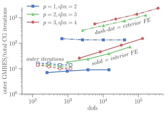
Figure 12: Outer GMRES(20) iterations to solve (37) and inner preconditioned CG iterations of interior/exterior FE problems for the quadratic-log problem.

5 Conclusions

We have demonstrated a method of coupling finite-element and integral equation solvers for the strong enforcement of boundary conditions on interior and exterior embedded boundaries. Furthermore, we have introduced a new method of coupling these FE-IE subproblems to solve a wide class of interface problems with homogeneous and non-homogeneous jump conditions. Our method does not require any special modifications to the finite element basis functions. It also does not need volume mesh refinement around the embedded domain, which means that time-dependent domains will not necessitate modifications to the volume-based finite element matrices—only the surface-based integral equation discretizations and the coupling matrices would be updated. One benefit is that our method can be implemented with off-the-shelf FE and IE packages. We have shown theoretical error bounds in the case of the interior embedded mesh problem and achieved empirical high-order convergence for interior, exterior, and interface examples, even very close to the embedded boundary.

References

- [1] H. A. Stone, Dynamics of drop deformation and breakup in viscous fluids, Annu. Rev. Fluid Mech 26 (1994) 65–102.
- [2] J. Parvizian, A. Düster, E. Rank, Finite cell method, Comput. Mech. 41 (2007) 121–133. doi:10.1007/s00466-007-0173-y.
- [3] S. Kollmannsberger, A. Özcan, J. Baiges, M. Ruess, E. Rank, A. Reali, Parameter-free, weak imposition of Dirichlet boundary conditions and coupling of trimmed and non-conforming patches, Int. J. Numer. Meth. Engng 101 (2015) 670–699. doi:10.1002/nme.
- [4] R. Glowinski, T.-W. Pan, J. Periaux, A fictitious domain method for Dirichlet problem and applications, Comput. Method Appl. M. 111 (1994) 283–303. doi:10.1016/0045-7825(94)90135-X.
- [5] L. Parussini, V. Pediroda, Fictitious Domain approach with -finite element approximation for incompressible fluid flow, J. Comp. Phys. 228 (2009) 3891–3910. doi:10.1016/j.jcp.2009.02.019.
- [6] R. J. LeVeque, Z. Li, The immersed interface method for elliptic equations with discontinuous coefficients and singular sources, SIAM J. Numer. Anal. 31 (1994) 1019–1044. doi:10.1137/0731054.
- [7] R. Mittal, G. Iaccarino, Immersed boundary methods, Annu. Rev. Fluid Mech. 37 (2005) 239–261.
- [8] Z. Li, The immersed interface method using a finite element formulation, Appl. Numer. Math. 27 (1998) 253–267.
- [9] Z. Li, T. Lin, X. Wu, New Cartesian grid methods for interface problems using the finite element formulation, Numer. Math. 96 (2003) 61–98.
- [10] Y. Gong, B. Li, Z. Li, Immersed-interface finite-element methods for elliptic interface problems with nonhomogeneous jump conditions, SIAM J. Numer. Anal. 46 (1) (2008) 472–495.
- [11] X. He, T. Lin, Y. Lin, Immersed finite element methods for elliptic interface problems with non-homogeneous interface problems, Int. J. Numer. Anal. Mod. 8 (2) (2011) 284–301.
- [12] R. Celorrio, V. Dominguez, F.-J. Sayas, Overlapped BEM–FEM and Some Schwarz Iterations, Computational Methods in Applied Mathematics Comput. Methods Appl. Math. 4 (1) (2004) 3–22. doi:10.2478/cmam-2004-0001.
- [13] V. Domínguez, F.-J. Sayas, Overlapped BEM–FEM for some Helmholtz transmission problems, Applied Numerical Mathematics 57 (2) (2007) 131–146. doi:10.1016/j.apnum.2006.02.001.
- [14] G. Biros, L. Ying, D. Zorin, A fast solver for the Stokes equations with distributed forces in complex geometries, J. Comp. Phys. 193 (2003) 317–348.
- [15] A. Mayo, The fast solution of Poisson’s and the biharmonic equations on irregular regions, SIAM J. Numer. Anal. 21 (2).
- [16] C. Johnson, J. C. Nedelec, On the coupling of boundary integral and finite element methods, Math. Comput. 35 (152) (1980) 1063–1079.
- [17] S. Meddahi, J. Valdés, O. Menéndez, P. Pérez, On the coupling of boundary integral and mixed finite element methods, J. Comput. Appl. Math. 69 (1996) 113–124.
- [18] A. Sequeira, The coupling of boundary integral and finite element methods for the bidimensional exterior steady stokes problem, Math. Methods Appl. Sci. 5 (1983) 356–375.
- [19] S. Meddahi, F.-J. Sayas, A fully discrete BEM-FEM for the exterior Stokes problem in the plane, SIAM J. Numer. Anal. 37 (6) (2000) 2082–2102.
- [20] M. Ganesh, C. Morgenstern, High-order FEM–BEM computer models for wave propagation in unbounded and heterogeneous media: Application to time-harmonic acoustic horn problem, J. Comput. Appl. Math. 307 (2016) 183–203.
- [21] M. E. Hassell, F.-J. Sayas, A fully discrete BEM–FEM scheme for transient acoustic waves, Comput. Methods Appl. Mech. Engrg. 309 (2016) 106–130.
- [22] T. Rüberg, F. Cirak, An immersed finite element method with integral equation correction, International Journal for Numerical Methods in Engineering 86 (1) (2010) 93–114. doi:10.1002/nme.3057.
- [23] N. Moës, J. Dolbow, T. Belytschko, A finite element method for crack growth without remeshing, International journal for numerical methods in engineering 46 (1) (1999) 131–150. doi:10.1002/(SICI)1097-0207(19990910)46:1<131::AID-NME726>3.0.CO;2-J.
- [24] T. Belytschko, N. Moës, S. Usui, C. Parimi, Arbitrary discontinuities in finite elements, International Journal for Numerical Methods in Engineering 50 (4) (2001) 993–1013. doi:10.1002/1097-0207(20010210)50:4<993::AID-NME164>3.0.CO;2-M.
- [25] K. W. Cheng, T.-P. Fries, Higher-order XFEM for curved strong and weak discontinuities, International Journal for Numerical Methods in Engineering 82 (5) (2010) 564–590. doi:10.1002/nme.2768.
- [26] S. Adjerid, T. Lin, A -th degree immersed finite element for boundary value problems with discontinuous coefficients, Appl. Numer. Math. 59 (2009) 1303–1321.
- [27] R. Kress, Linear Integral Equations, 3rd Edition, Springer Science+Business Media, New York, 2014.
- [28] T. Askham, A. J. Cerfon, An adaptive fast multipole accelerated poisson solver for complex geometries, Journal of Computational Physics 344 (2017) 1–22.
- [29] P. M. Anselone, R. Moore, Approximate solutions of integral and operator equations, Journal of Mathematical Analysis and Applications 9 (2) (1964) 268–277.
- [30] R. Haverkamp, Eine Aussage zur -Stabilität und zur genauen Konvergenzordnung der -Projektionen, Numerische Mathematik 44 (3) (1984) 393–405. doi:10.1007/BF01405570.
- [31] D. Leykekhman, B. Vexler, Finite Element Pointwise Results on Convex Polyhedral Domains, SIAM Journal on Numerical Analysis 54 (2) (2016) 561–587. doi:10.1137/15M1013912.
- [32] A. Klöckner, A. Barnett, L. Greengard, M. O’Neil, Quadrature by expansion: A new method for the evaluation of layer potentials, J. Comp. Phys. 252 (2013) 332–349.
-
[33]
A. Klöckner, pytential.
URL https://github.com/inducer/pytential - [34] M. Wala, A. Klöckner, A Fast Algorithm with Error Bounds for Quadrature by Expansion, ArXiv e-prints. Accepted for publication in Journal of Computational Physics. arXiv:1801.04070.
- [35] W. Bangerth, D. Davydov, T. Heister, L. Heltai, G. Kanschat, M. Kronbichler, M. Maier, B. Turcksin, D. Wells, The deal.II Library, Version 8.4, J. Numer. Math. 24.
- [36] W. Bangerth, R. Hartmann, G. Kanschat, deal.II – a general purpose object oriented finite element library, ACM Trans. Math. Softw. 33 (4) (2007) 24/1–24/27.
- [37] S. Brenner, L. R. Scott, The Mathematical Theory of Finite Element Methods, Springer Science & Business Media, 2013.
- [38] C. L. Epstein, L. Greengard, A. Klöckner, On the convergence of local expansions of layer potentials, SIAM J. Numer. Anal. 51 (5) (2013) 2660–2679.
- [39] R. Scott, Optimal estimates for the finite element method on irregular meshes, Math. Comput. 30 (136) (1976) 681–697.
- [40] A. H. Schatz, A weak discrete maximum principle and stability of the finite element method in on plane polygonal domains, Math. Comput. 34 (149) (1980) 77–91. doi:10.1090/S0025-5718-1980-0551291-3.
- [41] D. Gilbarg, N. S. Trudinger, Elliptic Partial Differential Equations of Second Order, Springer, 2015.
-
[42]
W. N. Bell, L. N. Olson, J. B. Schroder,
PyAMG: Algebraic multigrid solvers in
Python v3.0, release 3.2 (2015).
URL https://github.com/pyamg/pyamg