Finite difference methods for two and three dimensional fractional Laplacian with applications to solve the fractional reaction-diffusion equations

Abstract

In this paper, we propose an accurate finite difference method to discretize the two and three dimensional fractional Laplacian $(-\Delta)^{\frac{\alpha}{2}}$ in the hypersingular integral form and apply it to solve the fractional reaction-diffusion equations. The key idea of our method is to split the strong singular kernel function of the fractional Laplacian. Hence, we first formulate the fractional Laplacian as the weighted integral of a central difference quotient and then approximate it by the weighted trapezoidal rule. 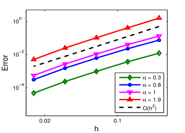It is proved that for $u\in C^{3,\frac{\alpha}{2}}({\mathbb{R}}^{d})$, our method has an accuracy of ${\mathcal{O}}(h^{2})$, uniformly for any $\alpha\in(0,2)$, while for $u\in C^{1,\frac{\alpha}{2}}({\mathbb{R}}^{d})$, the accuracy is ${\mathcal{O}}(h^{1-\frac{\alpha}{2}})$. As $\alpha\to 2^{-}$, the convergence behavior of our method is consistent with that of the central difference approximation of the classical Laplace operator. This study would fill the gap in the literature on numerical methods for the high dimensional factional Laplacian. In addition, we apply our method to solve the fractional reaction-diffusion equations and present a fast algorithm for their efficient computations. The computational cost of our method is ${\mathcal{O}}(M\log M)$, and the storage memory is ${\mathcal{O}}(M)$, with $M$ the total number of spatial unknowns. Moreover, our method is simple and easy to implement. 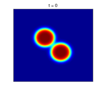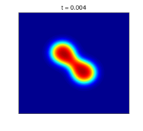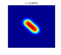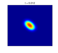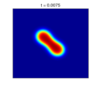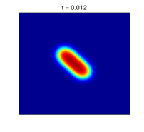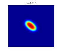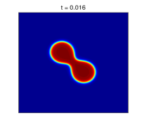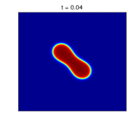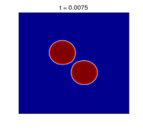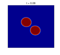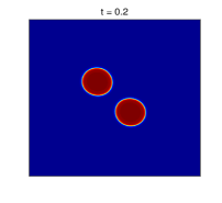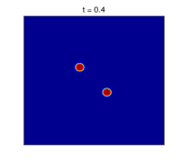Various examples, including the two-dimensional fractional Allen–Cahn equation, and two- and three-dimensional fractional Gray–Scott equations, are provided to demonstrate the effectiveness of our method. It shows that our method is accurate and efficient in solving the higher dimensional fractional reaction-diffusion equation, and it can be easily applied to solve other fractional PDEs.

Key words: Fractional Laplacian, finite difference methods, weighted trapezoidal rule, Montgomery identity, fractional Allan–Cahn equation, fractional Gray–Scott equations.

1 Introduction

The reaction-diffusion equation is one of the most applied partial differential equations (PDEs), and its applications can be found in many fields, including biology, chemistry, physics, finance, and so on. In classical reaction-diffusion equations, the diffusion is described by the standard Laplace operator $\Delta$, characterizing the transport mechanics due to the Brownian motion. Recently, it has been suggested that many complex (e.g., biological and chemical) systems are indeed characterized by the Lévy motion, rather than the Brownian motion; see [8, 13, 21, 6] and references therein. Hence, the classical reaction-diffusion models fail to properly describe the phenomena in these systems. To circumvent such issues, the fractional reaction-diffusion equations were proposed, where the classical Laplace operator is replaced by the fractional Laplacian $(-\Delta)^{\frac{\alpha}{2}}$ [21, 8]. In contrast to the classical diffusion models, the fractional models possess significant advantages for describing problems with long-range interactions, enabling one to describe the power law invasion profiles that have been observed in many applications [5, 22, 27].

Let $\Omega\in{\mathbb{R}}^{d}$ (for $d=1,2$, or $3$) be an open bounded domain, and $\Omega^{c}={\mathbb{R}}^{d}\backslash\Omega$ represents the complement of $\Omega$. We consider the following fractional reaction-diffusion equation:

$$\partial_{t}u({\bf x},t)=-\kappa_{d}(-\Delta)^{\frac{\alpha}{2}}u+f(u), \ {\bf x}\in\Omega,\quad\ t>0,$$ (1.1)

$$u({\bf x},t)=0, \ {\bf x}\in\Omega^{c},\quad\ t\geq 0,$$ (1.2)

$$u({\bf x},0)=g({\bf x}), \ {\bf x}\in\Omega,$$ (1.3)

where $\kappa_{d}>0$ denotes the diffusion coefficient. The fractional Laplacian $(-\Delta)^{\frac{\alpha}{2}}$ is defined by [18, 25]:

$$(-\Delta)^{\frac{\alpha}{2}}u({\bf x})=c_{d,\alpha}\ {\rm P.V.}\int_{\mathbb{R}^{d}}\frac{u({\bf x})-u({\bf x}^{\prime})}{|{\bf x}-{\bf x}^{\prime}|^{d+\alpha}}\,d{\bf x^{\prime}},\qquad\mbox{for \ $\alpha\in(0,2)$},$$ (1.4)

where P.V. stands for the Cauchy principal value, and $|{\bf x}-{\bf x}^{\prime}|$ denotes the Euclidean distance between points ${\bf x}$ and ${\bf x}^{\prime}$. The normalization constant $c_{d,\alpha}$ is defined as

$$c_{d,\alpha}=\frac{2^{\alpha-1}\alpha\,\Gamma\big{(}({d+\alpha})/{2}\big{)}}{\sqrt{\pi^{d}}\,\Gamma\big{(}\displaystyle 1-{\alpha}/{2}\big{)}},\qquad\mbox{for}\ \ \ d=1,2,3$$

with $\Gamma(\cdot)$ denoting the Gamma function. From a probabilistic point of view, the fractional Laplacian represents the infinitesimal generator of a symmetric $\alpha$-stable Lévy process. In the literature, the fractional Laplacian is also defined via a pseudo-differential operator with symbol $|{\bf k}|^{\alpha}$ [18, 25], i.e.,

$$(-\Delta)^{\frac{\alpha}{2}}u({{\bf x}})=\mathcal{F}^{-1}\big{[}|{\bf k}|^{\alpha}\mathcal{F}[u]\big{]},\qquad\mbox{for}\ \ \alpha>0,$$ (1.5)

where $\mathcal{F}$ represents the Fourier transform, and $\mathcal{F}^{-1}$ denotes its inverse. Over the entire space $\mathbb{R}^{d}$, the fractional Laplacian (1.4) is equivalent to the pseudo-differential operator (1.5) and many other fractional operators; see the discussion in [9, 25, 17, 11]. On the other hand, the rotational invariance of the fractional Laplacian (1.4) distinguishes it from the fractional Riemann–Liouville derivative when $d\geq 2$ [14]. In fact, the fractional Laplacian (1.4) is rotational invariant for $d\geq 1$, which is crucial in modeling the isotropic anomalous diffusion in many applications [16]. In this study, we focus on the fractional Laplacian in hypersingular integral form (1.4).

One main challenge in the study of the fractional reaction-diffusion equation (1.1)–(1.3) is to discretize the fractional Laplacian (1.4). Due to its hypersingularity, numerical methods for the fractional Laplacian (1.4) still remain scant. In [2], a finite element method is proposed to solve the one-dimensional (1D) fractional Poisson equation, and it is generalized to two-dimensional (2D) cases in [1]. A finite element method is used to solve the 2D Brusselator system on polygonal domains in [3]. In [28], a spectral Galerkin method is presented for the 1D reaction-diffusion equation. So far, several finite difference methods are proposed to discretize the fractional Laplacian (see [10] and references therein), but they are all limited to 1D cases. To the best of our knowledge, finite difference methods for high-dimensional (i.e., $d>1$) fractional Laplacian (1.4) are still missing in the literature. Moreover, no numerical method can be found for the three-dimensional (3D) fractional Laplacian.

In this paper, we propose an accurate and efficient finite difference method to discretize the two and three dimensional fractional Laplacian (1.4) and apply it to solve the fractional reaction-diffusion equation (1.1)–(1.3). Our method provides a fractional analogue of central difference schemes to the fractional Laplacian $(-\Delta)^{\frac{\alpha}{2}}$, and as $\alpha\to 2^{-}$, it reduces to the central difference scheme of the classical Laplace operator $-\Delta$. It could be a great tool to compare and understand the differences of mathematical models with the classical and fractional Laplacian. We prove that for $u\in C^{1,\frac{\alpha}{2}}({\mathbb{R}}^{d})$, our method has an accuracy of ${\mathcal{O}}(h^{1-\frac{\alpha}{2}})$, while for $u\in C^{3,\frac{\alpha}{2}}({\mathbb{R}}^{d})$, the accuracy increases to ${\mathcal{O}}(h^{2})$, uniformly for any $\alpha\in(0,2)$. Extensive numerical examples are provided to verify our analysis. Our study not only provides an accurate finite difference method for high-dimensional fractional Laplacian, but also fills the gap in the literature on numerical methods for 3D fractional Laplacian. On the other hand, it is well known that the computational costs of solving the fractional PDEs are forbiddingly expensive, due to the large and dense stiffness matrix. One merit of our method is that it results in a symmetric block Toeplitz matrix. Based on this property, we develop a fast algorithm via fast Fourier transform (FFT) to efficiently compute the fractional reaction-diffusion equations. Our algorithm has the computational complexity of ${\mathcal{O}}(M\log M)$, and memory storage ${\mathcal{O}}(M)$ with $M$ the total number of unknowns in space. Various examples, including the 2D fractional Allen–Cahn equation, and 2D and 3D fractional Gray–Scott equations are provided to demonstrate the effectiveness of our method.

This paper is organized as follows. In Sec. 2, we propose a finite difference method for the 2D fractional Laplacian, and the detailed error estimates are provided in Sec. 3. In Sec. 4, the discretization of the fractional reaction-diffusion equation (1.1)–(1.3) are presented together with the convergence analysis and efficient implementation. In Sec. 5, we generalize our results in Sec. 2–4 to 3D. Numerical examples are presented in Sec. 6 to test the accuracy of our method and study various fractional reaction-diffusion equations. Finally, we draw conclusions in Sec. 7.

2 Finite difference method for the fractional Laplacian

Due to its nonlocality, numerical methods for the fractional Laplacian still remain very limited, especially in high dimensions (i.e., $d>1$). Recently, several finite difference methods are proposed to discretize the 1D fractional Laplacian; see [10] and references therein. However, the finite difference method for the high-dimensional fractional Laplacian (1.4) is still missing in the literature. In this section, we present a finite difference method to discretize the 2D fractional Laplacian, and its generalization to 3D can be found in Sec. 5.

The key idea of our method is to reformulate the fractional Laplacian (1.4) as a weighted integral of the central difference quotient; see (2.3). This idea was first introduced in [10, 12] for the 1D fractional Laplacian, and it has been applied to solve the fractional Schrödinger equation in an infinite potential well [12]. Currently, the method in [10] is the state-of-the-art finite difference method for the 1D fractional Laplacian – it has a second order of accuracy uniformly for any $\alpha\in(0,2)$. However, the generalization of this scheme to high dimensions is not straightforward, especially numerical analysis. In the following, we will present a detailed scheme to the 2D fractional Laplacian (1.4), and its error estimates will be carried out in Sec. 3.

Let the domain $\Omega=(a_{x},b_{x})\times(a_{y},b_{y})$. First, we introduce new variables $\xi=|x-x^{\prime}|$ and $\eta=|y-y^{\prime}|$, denote the vector $\textit{{\boldmath$\xi$}}=(\xi,\eta)$, and then rewrite the 2D fractional Laplacian (1.4) as:

$$(-\Delta)^{\frac{\alpha}{2}}u({\bf x})=-c_{2,\alpha}\int_{0}^{\infty}\int_{0}^{\infty}\frac{1}{|\textit{{\boldmath$\xi$}}|^{2+\alpha}}\bigg{(}\sum_{m,n=0,1}u\big{(}x+(-1)^{m}\xi,\,y+(-1)^{n}\eta\big{)}-4u({\bf x})\bigg{)}d\xi d\eta.$$ (2.1)

This is a hypersingular integral, and the traditional quadrature rule can not provide a satisfactory approximation [20]. Here, we introduce a splitting parameter $\gamma\in(\alpha,2]$, and define a function

$$\psi_{\gamma}({\bf x},\textit{{\boldmath$\xi$}}):=\Big{(}\sum_{m,n=0,1}u\big{(}x+(-1)^{m}\xi,\,y+(-1)^{n}\eta\big{)}-4u({\bf x})\Big{)}|\textit{{\boldmath$\xi$}}|^{-\gamma}.$$ (2.2)

Then, the fractional Laplacian in (2.1) can be further written as

$$(-\Delta)^{\frac{\alpha}{2}}u({\bf x})=-c_{2,\alpha}\int_{0}^{\infty}\int_{0}^{\infty}\psi_{\gamma}({\bf x},\textit{{\boldmath$\xi$}})\omega_{\gamma}(\textit{{\boldmath$\xi$}})\,d\xi d\eta,$$ (2.3)

i.e., a weighted integral of the central difference quotient $\psi_{\gamma}$ with the weight function $\omega_{\gamma}(\textit{{\boldmath$\xi$}})=|\textit{{\boldmath$\xi$}}|^{\gamma-(2+\alpha)}$. The reformulation in (2.3), i.e., splitting the kernel function and rewriting it as a weighted integral, is the key idea of our method. Note that the splitting parameter $\gamma$ plays a crucial role in determining the accuracy of our method, which will be discussed further in Sec. 3.

Choose a constant $L=\max\{b_{x}-a_{x},\,b_{y}-a_{y}\}$, and denote $D_{1}=(0,L)^{2}$ and $D_{2}={\mathbb{R}}^{2}_{+}\backslash D_{1}=\{(\xi,\eta)\mid\xi,\eta>0,\ \mbox{but}\ (\xi,\eta)\notin D_{1}\}$. We can divide the integration domain of (2.3) into two parts:

$$(-\Delta)^{\frac{\alpha}{2}}u({\bf x})=-c_{2,\alpha}\bigg{(}\int_{D_{1}}\psi_{\gamma}({\bf x},\,\textit{{\boldmath$\xi$}})\omega_{\gamma}(\textit{{\boldmath$\xi$}})\,d\xi d\eta+\int_{D_{2}}\psi_{\gamma}({\bf x},\,\textit{{\boldmath$\xi$}})\omega_{\gamma}(\textit{{\boldmath$\xi$}})\,d\xi d\eta\bigg{)}.$$ (2.4)

Due to the extended homogeneous Dirichlet boundary condition (1.2), the second integral of (2.4) can be easily simplified. Notice that for ${\bf x}\in\Omega$, and $\xi\geq L$ or $\eta\geq L$, the point $(x+(-1)^{m}\xi,y+(-1)^{n}\eta)\in\Omega^{c}$, for $m,n=0,1$, and thus $u(x+(-1)^{m}\xi,y+(-1)^{n}\eta)=0$. Immediately, we can reduce the function $\psi_{\gamma}({\bf x},\textit{{\boldmath$\xi$}})=-4u({\bf x})|\textit{{\boldmath$\xi$}}|^{-\gamma}$ on $D_{2}$, and simplify the integral over $D_{2}$ as:

$$\int_{D_{2}}\psi_{\gamma}({\bf x},\,\textit{{\boldmath$\xi$}})\,\omega_{\gamma}(\textit{{\boldmath$\xi$}})\,d\xi d\eta=-4u({\bf x})\int_{D_{2}}|\textit{{\boldmath$\xi$}}|^{-(2+\alpha)}\,d\xi d\eta,$$ (2.5)

If the integral of $|\textit{{\boldmath$\xi$}}|^{-(2+\alpha)}$ over $D_{2}$ can be evaluated exactly, the calculation of the second term of (2.4) is exact, and no discretization errors are introduced. We now move to approximate the first integral of (2.4). Here, the main difficulty comes from the strong singular kernel, and we propose a weighted trapezoidal method to retain part of the singularity in the integral. Choose an integer $N>0$, and define the mesh size $h=L/N$. Denote grid points $\xi_{i}=ih$ and $\eta_{j}=jh$, for $0\leq i,j\leq N$. For notational simplicity, we denote $\textit{{\boldmath$\xi$}}_{ij}=(\xi_{i},\,\eta_{j})$ and then $|\textit{{\boldmath$\xi$}}_{ij}|=\sqrt{\xi_{i}^{2}+\eta_{j}^{2}}$, for $0\leq i,\,j\leq N$. Additionally, we define the element ${I}_{ij}:=[ih,\,(i+1)h]\times[jh,(j+1)h]$, for $0\leq i,\,j\leq N-1$. It is easy to see that $D_{1}=\cup_{i,j=0}^{N-1}\,I_{ij}$, and thus we can formulate the first integral of (2.4) as:

$$\int_{D_{1}}\psi_{\gamma}({\bf x},\textit{{\boldmath$\xi$}})\omega_{\gamma}(\textit{{\boldmath$\xi$}})\,d\xi d\eta=\sum_{i,j=0}^{N-1}\int_{{I}_{ij}}\psi_{\gamma}({\bf x},\textit{{\boldmath$\xi$}})\omega_{\gamma}(\textit{{\boldmath$\xi$}})\,d\xi d\eta.$$ (2.6)

Next, we focus on the approximation to the integral over each element $I_{ij}$. For $i\neq 0$ or $j\neq 0$, we use the weighted trapezoidal rule and obtain the approximation:

$$\int_{I_{ij}}\psi_{\gamma}({\bf x},\textit{{\boldmath$\xi$}})\omega_{\gamma}(\textit{{\boldmath$\xi$}})\,d\xi d\eta\approx\frac{1}{4}\bigg{(}\sum_{m,n=0,1}\psi_{\gamma}\big{(}{\bf x},\textit{{\boldmath$\xi$}}_{(i+m)(j+n)}\big{)}\bigg{)}\int_{I_{ij}}\omega_{\gamma}(\textit{{\boldmath$\xi$}})\,d\xi d\eta,$$ (2.7)

While $i=j=0$, the approximation of the integral over $I_{00}$ is not as straightforward as that in (2.7). Using the weighted trapezoidal rule, we get

$$\int_{I_{00}}\psi_{\gamma}({\bf x},\textit{{\boldmath$\xi$}})\omega_{\gamma}(\textit{{\boldmath$\xi$}})\,d\xi d\eta\approx\frac{1}{4}\bigg{(}\lim_{\textit{{\boldmath$\xi$}}\rightarrow{\bf 0}}\psi_{\gamma}\big{(}{\bf x},\,{\textit{{\boldmath$\xi$}}}\big{)}+\sum_{\begin{subarray}{c}m,n=0,1\\ m+n\neq 0\end{subarray}}\psi_{\gamma}\big{(}{\bf x},\textit{{\boldmath$\xi$}}_{(i+m)(j+n)}\big{)}\bigg{)}\int_{I_{00}}\omega_{\gamma}(\textit{{\boldmath$\xi$}})\,d\xi d\eta.$$ (2.8)

Assuming the limit in (2.8) exists, then it depends on the splitting parameter $\gamma$. We will divide our discussion into two cases: $\gamma\in(\alpha,2)$ and $\gamma=2$. If $\gamma=2$, it is approximated by:

$$\lim_{\textit{{\boldmath$\xi$}}\rightarrow{\bf 0}}\psi_{2}({\bf x},\,{\textit{{\boldmath$\xi$}}})\approx\psi_{2}({\bf x},\,{\textit{{\boldmath$\xi$}}}_{10})+\psi_{2}({\bf x},\,{\textit{{\boldmath$\xi$}}}_{01})-\psi_{2}({\bf x},\,{\textit{{\boldmath$\xi$}}}_{11}),\quad\ \ \mbox{if}\ \ \gamma=2;$$ (2.9)

while $\gamma\in(\alpha,2)$, we have

$$\lim_{\textit{{\boldmath$\xi$}}\rightarrow{\bf 0}}\psi_{\gamma}({\bf x},\,{\textit{{\boldmath$\xi$}}})=\lim_{\textit{{\boldmath$\xi$}}\rightarrow{\bf 0}}\big{(}\psi_{2}({\bf x},\,{\textit{{\boldmath$\xi$}}})|\textit{{\boldmath$\xi$}}|^{2-\gamma}\big{)}=0,\quad\ \ \mbox{if}\ \ \gamma\in(\alpha,2).$$ (2.10)

Substituting (2.9)–(2.10) into (2.8), we obtain the approximation of the integral over $I_{00}$ as:

$$\int_{I_{00}}\psi_{\gamma}({\bf x},\textit{{\boldmath$\xi$}})\omega_{\gamma}(\textit{{\boldmath$\xi$}})\,d\xi d\eta\approx\frac{1}{4}\bigg{(}\sum_{\begin{subarray}{c}m,n=0,1\\ m+n\neq 0\end{subarray}}c_{mn}^{\gamma}\,\psi_{\gamma}\big{(}{\bf x},\textit{{\boldmath$\xi$}}_{(i+m)(j+n)}\big{)}\bigg{)}\int_{I_{00}}\omega_{\gamma}(\textit{{\boldmath$\xi$}})\,d\xi d\eta,\ \$$ (2.11)

where $c_{mn}^{\gamma}=1$ for $\gamma\in(\alpha,2)$, while $c_{10}^{\gamma}=c_{01}^{\gamma}=2$ and $c_{11}^{\gamma}=0$ for $\gamma=2$. Denote all the elements associated to the point $\textit{{\boldmath$\xi$}}_{ij}$, i.e., elements that have $\textit{{\boldmath$\xi$}}_{ij}$ as a vertex, as:

$${T}_{ij}=\big{(}{I}_{(i-1)(j-1)}\cup{I}_{(i-1)j}\cup{I}_{i(j-1)}\cup{I}_{ij}\big{)}\cap D_{1},\quad\ \ \mbox{for}\ \ 0\leq i,\,j\leq N-1.$$

Then, combining (2.4)–(2.7) and (2.11) and reorganizing the terms, we obtain the approximation to the 2D fractional Laplacian (1.4) as:

$$(-\Delta)_{h,\gamma}^{\frac{\alpha}{2}}u({\bf x})=-\frac{c_{2,\alpha}}{4}\bigg{(}\left\lfloor\frac{\gamma}{2}\right\rfloor\Big{(}\psi_{\gamma}\big{(}{\bf x},\,{\textit{{\boldmath$\xi$}}}_{10}\big{)}+\psi_{\gamma}\big{(}{\bf x},\,{\textit{{\boldmath$\xi$}}}_{01}\big{)}-\psi_{\gamma}\big{(}{\bf x},\,{\textit{{\boldmath$\xi$}}}_{11}\big{)}\Big{)}\int_{I_{00}}\omega_{\gamma}(\textit{{\boldmath$\xi$}})\,d\xi d\eta\qquad\qquad$$

$$\hskip 85.35826pt+\bigg{(}{\sum_{\begin{subarray}{c}i,j=0\\ i+j\neq 0\end{subarray}}^{N-1}}\psi_{\gamma}\big{(}{\bf x},\,\textit{{\boldmath$\xi$}}_{ij}\big{)}\bigg{)}\int_{T_{ij}}\omega_{\gamma}(\textit{{\boldmath$\xi$}})\,d\xi d\eta-16u({\bf x})\int_{D_{2}}|\textit{{\boldmath$\xi$}}|^{-(2+\alpha)}d\xi d\eta\bigg{)},$$ (2.12)

with $\lfloor\cdot\rfloor$ denoting the floor function.

Without loss of generality, we assume that $N_{x}=N$, and choose $N_{y}$ as the smaller integer such that $a_{y}+N_{y}h\geq b_{y}$. Define the grid points $x_{i}=a_{x}+ih$ for $0\leq i\leq N_{x}$, and $y_{j}=a_{y}+jh$ for $0\leq j\leq N_{y}$. Let $u_{ij}$ be the numerical approximation of $u(x_{i},y_{j})$. Noticing the definition of $\psi_{\gamma}$ in (2.2), we get the fully discretized 2D fractional Laplacian as:

$$(-\Delta)_{h,\gamma}^{\frac{\alpha}{2}}u_{ij}=-c_{2,\alpha}\bigg{[}a_{00}u_{ij}+\sum_{m=0}^{i-1}\bigg{(}\sum_{\begin{subarray}{c}n=0\\ m+n\neq 0\end{subarray}}^{j-1}a_{mn}u_{(i-m)(j-n)}+\sum_{n=1}^{N_{y}-1-j}a_{mn}u_{(i-m)(j+n)}\bigg{)}\qquad\qquad$$

$$\hskip 71.13188pt+\sum_{m=0}^{N_{x}-1-i}\bigg{(}\sum_{\begin{subarray}{c}n=0\\ m+n\neq 0\end{subarray}}^{j-1}a_{mn}u_{(i+m)(j-n)}+\sum_{n=1}^{N_{y}-1-j}a_{mn}u_{(i+m)(j+n)}\bigg{)}\bigg{]},$$ (2.13)

for $1\leq i\leq N_{x}-1$ and $1\leq j\leq N_{y}-1$. The scheme (2) shows that the discretized fractional Laplacian at point $(x_{i},y_{j})$ depends on all points in the domain $\Omega$, reflecting the nonlocal characteristic of the fractional Laplacian. The coefficient $a_{mn}$ depends on the choice of the splitting parameter $\gamma$. For $m,n\geq 0$ but $m+n>0$, there is

$$a_{mn}=\frac{2^{\sigma(m,n)}}{4|\textit{{\boldmath$\xi$}}_{mn}|^{\gamma}}\bigg{(}\int_{T_{mn}}|\textit{{\boldmath$\xi$}}|^{\gamma-(2+\alpha)}\,d\xi d\eta+\bar{c}_{mn}\left\lfloor\frac{\gamma}{2}\right\rfloor\int_{T_{00}}|\textit{{\boldmath$\xi$}}|^{\gamma-(2+\alpha)}\,d\xi d\eta\bigg{)},\qquad$$ (2.14)

where $\sigma(m,n)$ denotes the number of zeros of $m$ and $n$, and the constant $\bar{c}_{01}=\bar{c}_{10}=-\bar{c}_{11}=1$, and $\bar{c}_{mn}\equiv 0$ for other $m,n$. For $m=n=0$, the coefficient

$$a_{00}=-2\sum_{m=1}^{N}\big{(}a_{m0}+a_{0m}\big{)}-4\sum_{m,n=1}^{N}a_{mn}-4\int_{D_{2}}|\textit{{\boldmath$\xi$}}|^{-(2+\alpha)}\,d\xi d\eta.$$ (2.15)

Remark 2.1.

Our extensive simulations show that $\gamma=2$ is the optimal splitting parameter, leading to the smallest errors. Moreover, as $\alpha\to 2^{-}$, our finite difference scheme in (2) with $\gamma=2$ reduces to the central difference scheme of the classical Laplace operator $-\Delta$. To show it, we notice that $a_{10}=a_{01}$ in (2.14), and when $\gamma=2$,

$$\lim_{\alpha\to 2^{-}}\big{(}c_{2,\alpha}a_{10}\big{)}=\frac{1}{h^{2}};\quad\ \lim_{\alpha\to 2^{-}}\big{(}c_{2,\alpha}a_{00}\big{)}=-\frac{4}{h^{2}};\quad\ \lim_{\alpha\to 2^{-}}\big{(}c_{2,\alpha}a_{mn}\big{)}=0,\ \ \mbox{for}\ \,m+n>0,$$

due to the following properties:

$$\lim_{\alpha\to 2^{-}}\bigg{(}c_{2,\alpha}\int_{I_{00}}|\textit{{\boldmath$\xi$}}|^{-\alpha}d\textit{{\boldmath$\xi$}}\bigg{)}=1,\qquad\lim_{\alpha\to 2^{-}}\bigg{(}c_{2,\alpha}\int_{I_{mn}}|\textit{{\boldmath$\xi$}}|^{-\alpha}d\textit{{\boldmath$\xi$}}\bigg{)}=0,\ \ \mbox{for}\ \,m+n>0.$$

We can write the scheme (2) into matrix-vector form. Denote the vector ${\bf u}_{x,j}=(u_{1,j},u_{2,j},\ldots,u_{N_{x}-1,j})$ for $1\leq j\leq N_{y}-1$, and let the block vector ${\bf u}=({\bf u}_{x,1},{\bf u}_{x,2},\,\ldots,{\bf u}_{x,\,N_{y}-1})^{T}$. Then the matrix-vector form of the scheme (2) is given by

$$(-\Delta)^{\frac{\alpha}{2}}_{h,\gamma}{\bf u}=A_{2}{\bf u},$$ (2.16)

where the matrix $A_{2}$ is a symmetric block Toeplitz matrix, defined as

$${{A_{2}}}=\left(\begin{array}[]{cccccc}A_{x,0}&A_{x,1}&\ldots&A_{x,N_{y}-3}&A_{x,N_{y}-2}\\ A_{x,1}&A_{x,0}&A_{x,1}&\cdots&A_{x,N_{y}-3}\\ \vdots&\ddots&\ddots&\ddots&\vdots\\ A_{x,N_{y}-3}&\ldots&A_{x,1}&A_{x,0}&A_{x,1}\\ A_{x,N_{y}-2}&A_{x_{1},N_{y}-3}&\ldots&A_{x,1}&A_{x,0}\end{array}\right)_{M\times M}$$ (2.22)

with $M=(N_{x}-1)(N_{y}-1)$ being the total number of unknowns, and each block $A_{x,j}$ (for $0\leq j\leq N_{y}-2$) is a symmetric Toeplitz matrix, defined as

$${A}_{x,j}=-c_{2,\alpha}\left(\begin{array}[]{cccccc}a_{0j}&a_{1j}&\ldots&a_{(N_{x}-3)j}&a_{(N_{x}-2)j}\\ a_{1j}&a_{0j}&a_{1j}&\cdots&a_{(N_{x}-3)j}\\ \vdots&\ddots&\ddots&\ddots&\vdots\\ a_{(N_{x}-3)j}&\ldots&a_{1j}&a_{0j}&a_{1j}\\ a_{(N_{x}-2)j}&a_{N_{x}-3j}&\ldots&a_{1j}&a_{0j}\end{array}\right)_{(N_{x}-1)\times(N_{x}-1)}.$$ (2.28)

It is easy to verify that the matrix $A_{2}$ is positive definite. In contrast to the differentiation matrix of the classical Laplacian, the matrix $A_{2}$ in (2.22) is a large dense matrix, which causes considerable challenges not only for storing the matrix but also for computing matrix-vector products. However, noticing that $A_{2}$ is a block-Toeplitz-Toeplitz-block matrix, we can develop a fast algorithm for the matrix-vector multiplication in (2.16). More details can be found in Sec. 4.

3 Error analysis for spatial discretization

In this section, we provide the error estimates for our finite difference method in discretizing the 2D fractional Laplacian. The main technique used in our proof is an extension of the weighted Montgomery identity (see Lemma 3.1). The Montgomery identity is the framework of developing many classical inequalities, such as the Ostrowski, Chebyshev, and Grüss type inequalities. As an extension, the weighted Montgomery identity, first introduced in [24, 15], plays an important role in the study of weighted integrals. Here, we will begin with introducing the following function:

Definition 3.1.

Let $w:[a,b]\times[c,\,d]\to{\mathbb{R}}$ be an integrable function. For $m,n\in{\mathbb{N}}^{0}$, define

$$\Theta_{[a,\,b]\times[c,\,d]}^{(m,n)}(x,y)=\sum_{(s,t)\in S}\int_{t}^{y}\int_{s}^{x}w(\xi,\eta)\,\frac{(x-{\xi})^{m}(y-{\eta})^{n}}{m!\ n!}\,d{\xi}d{\eta},\quad\ \,(x,y)\in[a,\,b]\times[c,\,d],$$

where the set $S=\big{\{}(a,c),(a,d),(b,c),(b,d)\big{\}}$.

The function $\Theta$ can be viewed as an extension of the generalized Peano kernel, and it has the following properties:

Property 3.1.

Let $m,n\in{\mathbb{N}}^{0}$, and $(x,y)\in[a,\,b]\times[c,\,d]$.

(i)  If $w(x,y)=w(y,x)$, then

$$\Theta_{[a,\,b]\times[c,\,d]}^{(m,n)}(x,y)=\Theta_{[c,\,d]\times[a,\,b]}^{(n,m)}(y,x).$$

(ii)   There exists a positive constant $C$, such that

$$\big{|}\Theta_{[a,\,b]\times[c,\,d]}^{(m,n)}(x,y)\big{|}\leq C(b-a)^{m}(d-c)^{n}\int_{c}^{d}\int_{a}^{b}w(\xi,\eta)\,d\xi d\eta$$

(iii)  For $0\leq k\leq m$ and $0\leq l\leq n$, there is

$$\partial_{k,l}\Theta^{(m,n)}_{[a,b]\times[c,d]}(x,y)=\Theta^{(m-k,\,n-l)}_{[a,b]\times[c,d]}(x,y).$$

Here, we denote $\partial_{m,n}f(x,y)=\partial_{x}^{m}\partial_{y}^{n}f(x,y)$ as a partial derivative of $f$.

The properties (i) and (ii) are implied from its definition, and the property (iii) can be obtained by using the Leibniz integral rule. Here, we will omit their proofs for brevity. Next, we introduce the following lemma from the weighted Montgomery identity of two variables.

Lemma 3.1 (Extension of the weighted Montgomery identity).

Let $w,f:[a,\,b]\times[c,\,d]\rightarrow\mathbb{R}$ be integrable functions. (i)   If the derivatives $\partial_{0,1}f$ and $\partial_{1,0}f$ exist and are integrable, there is

$$\int_{c}^{d}\int_{a}^{b}\Big{(}4f(x,y)-\big{(}f(a,c)+f(a,d)+f(b,c)+f(b,d)\big{)}\Big{)}w(x,y)\,dxdy$$

$$\hskip 14.22636pt=-\frac{1}{2}\int_{c}^{d}\int_{a}^{b}\left(\partial_{0,1}\Theta_{[a,\,b]\times[c,\,d]}^{(0,0)}(x,y)\,\partial_{1,0}f(x,y)+\partial_{1,0}\Theta_{[a,\,b]\times[c,\,d]}^{(0,0)}(x,y)\,\partial_{0,1}f(x,y)\right)dxdy$$

$$\hskip 25.6073pt-\frac{1}{2}\int_{a}^{b}\left(\Theta_{[a,\,b]\times[c,\,d]}^{(0,0)}(x,d)\,\partial_{1,0}f(x,d)-\Theta_{[a,\,b]\times[c,\,d]}^{(0,0)}(x,c)\,\partial_{1,0}f(x,c)\right)dx$$

$$\hskip 25.6073pt-\frac{1}{2}\int_{c}^{d}\left(\Theta_{[a,\,b]\times[c,\,d]}^{(0,0)}(b,y)\,\partial_{0,1}f(b,y)-\Theta_{[a,\,b]\times[c,\,d]}^{(0,0)}(a,y)\,\partial_{0,1}f(a,y)\right)dy.\qquad\qquad\qquad\qquad$$

(ii)   If the derivatives $\partial_{m,2}f$ and $\partial_{2,n}f$ exist and are integrable, for $m,n=0,1$, there is

$$\int_{c}^{d}\int_{a}^{b}\Big{(}4f(x,y)-\big{(}f(a,c)+f(a,d)+f(b,c)+f(b,d)\big{)}\Big{)}w(x,y)\,dxdy$$

$$\hskip 14.22636pt=-\frac{1}{2}\int_{c}^{d}\int_{a}^{b}\left(\Theta_{[a,\,b]\times[c,\,d]}^{(0,1)}(x,y)\,\partial_{1,2}f(x,y)+\Theta_{[a,\,b]\times[c,\,d]}^{(1,0)}(x,y)\,\partial_{2,1}f(x,y)\right)dxdy$$

$$\hskip 25.6073pt+\sum_{n=0,1}\left(-\frac{1}{2}\right)^{n}\bigg{(}\int_{a}^{b}\left(\Theta_{[a,\,b]\times[c,\,d]}^{(1,n)}(x,d)\partial_{2,n}f(x,d)-\Theta_{[a,\,b]\times[c,\,d]}^{(1,n)}(x,c)\partial_{2,n}f(x,c)\right)dx\qquad\qquad\qquad$$

$$\hskip 96.73918pt+\int_{c}^{d}\left(\Theta_{[a,\,b]\times[c,\,d]}^{(n,1)}(b,y)\partial_{n,2}f(b,y)-\Theta_{[a,\,b]\times[c,\,d]}^{(n,1)}(a,y)\partial_{n,2}f(a,y)\right)dy\bigg{)}$$

$$\hskip 25.6073pt+\sum_{\begin{subarray}{c}m,n=0,1\\ m+n\neq 0\end{subarray}}(-1)^{m+n}\left(\Theta_{[a,\,b]\times[c,\,d]}^{(m,n)}(b,d)\,\partial_{m,n}f(b,d)-\Theta_{[a,\,b]\times[c,\,d]}^{(m,n)}(b,c)\,\partial_{m,n}f(b,c)\right.$$

$$\hskip 113.81102pt-\Theta_{[a,\,b]\times[c,\,d]}^{(m,n)}(a,d)\partial_{m,n}f(a,d)+\Theta_{[a,\,b]\times[c,\,d]}^{(m,n)}(a,c)\partial_{m,n}f(a,c)\Big{)}.$$

Proof.

The proof of Lemma 3.1 can be done by first averaging the wighted Montgomery identity [15, Theorem 2.2] at points $(a,c)$, $(a,d)$, $(b,c)$ and $(b,d)$, and then using the integration by parts. ∎

The Chebyshev integral inequality for two-variable functions will be frequently used in the proof of our theorems. For the sake of completeness, we will review it as follows, and the Chebyshev integral inequality for multiple variable functions can be found in [4, Theorem A].

Lemma 3.2 (Chebyshev integral inequality).

Let $f,g:[a,b]\times[c,d]\to{\mathbb{R}}$ be continuous, nonnegative, and similarly ordered, i.e., $\big{(}f(x_{1},y_{1})-f(x_{2},y_{2})\big{)}\big{(}g(x_{1},y_{1})-g(x_{2},y_{2})\big{)}\geq 0$, for any points $(x_{1},y_{1})$ and $(x_{2},y_{2})$. Then, there is

$$\bigg{(}\int_{c}^{d}\int_{a}^{b}f(x,y)\,dxdy\bigg{)}\bigg{(}\int_{c}^{d}\int_{a}^{b}g(x,y)\,dxdy\bigg{)}\leq(b-a)(d-c)\int_{c}^{d}\int_{a}^{b}f(x,y)g(x,y)\,dxdy.$$

Definition 3.2.

For $k\in{\mathbb{N}}^{0}$ and $\alpha\in(0,2]$, let $C^{k,\frac{\alpha}{2}}({\mathbb{R}}^{d})$ denote the space that consists of all functions $u:{\mathbb{R}}^{d}\to{\mathbb{R}}$ with continuous partial derivatives of order less than or equal to $k$, whose $k$-th partial derivatives are uniformly Hölder continuous with exponent $\frac{\alpha}{2}$.

To prepare our main theorems, we will first study the properties of function $\psi_{\gamma}({\bf x},\textit{{\boldmath$\xi$}})$. For notational simplicity, we will omit ${\bf x}$, and let $\psi_{\gamma}({\textit{{\boldmath$\xi$}}}):=\psi_{\gamma}({\bf x},\textit{{\boldmath$\xi$}})$.

Lemma 3.3.

Let $\alpha\in(0,2)$ and $(\xi,\eta)\in{\mathbb{R}}^{2}\backslash\{\bf 0\}$.

• If $u\in C^{1,\frac{\alpha}{2}}(\mathbb{R}^{2})$, then the derivative $\partial_{m,n}\psi_{\gamma}$ exists, for $m,n=0,1$ and $m+n<2$. Moreover, there exists a positive constant $C$, such that

  $$\Big{|}\partial_{m,n}\psi_{\gamma}(\xi,\eta)\Big{|}\leq C|\textit{{\boldmath$\xi$}}|^{\frac{\alpha}{2}+1-\gamma-(m+n)},\qquad\mbox{for \ $\gamma\in(\alpha,2]$}.$$

• If $u\in C^{3,\frac{\alpha}{2}}(\mathbb{R}^{2})$, then the derivative $\partial_{m,n}\psi_{2}(\xi,\eta)$ exists, for $m,n=0,1,2$ and $0<m+n<4$. Moreover, there is

  $$\big{|}\partial_{m,n}\psi_{2}(\xi,\eta)+\partial_{n,m}\psi_{2}(\eta,\xi)\big{|}\leq C|\textit{{\boldmath$\xi$}}|^{\frac{\alpha}{2}+1-(m+n)},$$

  with $C$ a positive constant. If one of $\xi$ and $\eta$ equals to zero, we further have

  $$\big{|}\partial_{1,0}\psi_{2}(\xi,0)\big{|}\leq C\xi^{\frac{\alpha}{2}},\qquad\big{|}\partial_{0,1}\psi_{2}(0,\eta)\big{|}\leq C\eta^{\frac{\alpha}{2}}.$$

Proof.

The proof of the above properties can be done by directly applying the Taylor’s theorem. ∎

Theorem 3.1.

Suppose that $u\in C^{1,\frac{\alpha}{2}}(\mathbb{R}^{2})$ has finite support on the domain $\Omega\in{\mathbb{R}}^{2}$. Let $(-\Delta)_{h,\gamma}^{\frac{\alpha}{2}}$ be the finite difference approximation of the fractional Laplacian $(-\Delta)^{\frac{\alpha}{2}}$, with $h$ a small mesh size. For any $\gamma\in(\alpha,2]$, the local truncation error

$$\big{\|}(-\Delta)^{\frac{\alpha}{2}}u({\bf x})-(-\Delta)^{\frac{\alpha}{2}}_{h,\gamma}u({\bf x})\big{\|}_{\infty}\leq Ch^{1-\frac{\alpha}{2}},\qquad\mbox{for}\ \ \alpha\in(0,2)$$ (3.1)

with $C$ a positive constant depending on $\alpha$ and $\gamma$.

Proof.

Introduce the error function at point ${\bf x}\in\Omega$ as:

$$e_{\alpha,\gamma}^{h}({\bf x}) = (-\Delta)^{\frac{\alpha}{2}}u({\bf x})-(-\Delta)^{\frac{\alpha}{2}}_{h,\gamma}u({\bf x})$$ (3.2)

$$= -\frac{c_{2,\alpha}}{4}\bigg{[}\int_{I_{00}}\Big{(}4\psi_{\gamma}(\textit{{\boldmath$\xi$}})-\sum_{\begin{subarray}{c}m,n=0,1\\ m+n\neq 0\end{subarray}}c_{mn}^{\gamma}\psi_{\gamma}\big{(}\textit{{\boldmath$\xi$}}_{mn}\big{)}\Big{)}w_{\gamma}(\textit{{\boldmath$\xi$}})d\xi d\eta$$

$$+\sum_{(i,j)\in\varkappa}\int_{I_{ij}}\Big{(}4\psi_{\gamma}(\textit{{\boldmath$\xi$}})-\sum_{m,n=0,1}\psi_{\gamma}\big{(}\textit{{\boldmath$\xi$}}_{(i+m)(j+n)}\big{)}\Big{)}w_{\gamma}(\textit{{\boldmath$\xi$}})d\xi d\eta\bigg{]},\qquad\$$

which is obtained from (2.4) and (2). For simplicity, we denote the index set

$$\varkappa=\big{\{}(i,j)\,|\,i,j=0,1,\ldots,N-1,\ \mbox{but}\ i+j\neq 0\big{\}}$$

Using Lemma 3.1 (i) to the last line of (3.2) with $w(\textit{{\boldmath$\xi$}})=|\textit{{\boldmath$\xi$}}|^{\gamma-(2+\alpha)}$, we further get

$$e_{\alpha,\gamma}^{h}({\bf x}) = -\frac{c_{2,\alpha}}{4}\bigg{[}\int_{I_{00}}\Big{(}4\psi_{\gamma}(\textit{{\boldmath$\xi$}})-\big{(}c_{10}^{\gamma}\psi_{\gamma}(\textit{{\boldmath$\xi$}}_{10})+c_{01}^{\gamma}\psi_{\gamma}(\textit{{\boldmath$\xi$}}_{01})+c_{11}^{\gamma}\psi_{\gamma}(\textit{{\boldmath$\xi$}}_{11})\big{)}\Big{)}|\textit{{\boldmath$\xi$}}|^{\gamma-(2+\alpha)}d\xi d\eta\qquad$$ (3.3)

$$\hskip 14.22636pt-\frac{1}{2}\sum_{(i,\,j)\in\varkappa}\int_{I_{ij}}\Big{(}\partial_{0,1}\Theta_{I_{ij}}^{(0,0)}(\xi,\eta)\,\partial_{1,0}\psi_{\gamma}(\xi,\eta)+\partial_{1,0}\Theta_{I_{ij}}^{(0,0)}(\xi,\eta)\,\partial_{0,1}\psi_{\gamma}(\xi,\eta)\Big{)}\,d\xi d\eta$$

$$\hskip 14.22636pt-\frac{1}{2}\sum_{(i,\,j)\in\varkappa}\int_{\xi_{i}}^{\xi_{i+1}}\Big{(}\Theta_{I_{ij}}^{(0,0)}(\xi,\eta_{j+1})\,\partial_{1,0}\psi_{\gamma}(\xi,\eta_{j+1})-\Theta_{I_{ij}}^{(0,0)}(\xi,\eta_{j})\,\partial_{1,0}\psi_{\gamma}(\xi,\eta_{j})\Big{)}d\xi$$

$$\hskip 14.22636pt-\frac{1}{2}\sum_{(i,\,j)\in\varkappa}\int_{\eta_{j}}^{\eta_{j+1}}\Big{(}\Theta_{I_{ij}}^{(0,0)}(\xi_{i+1},\eta)\,\partial_{0,1}\psi_{\gamma}(\xi_{i+1},\eta)-\Theta_{I_{ij}}^{(0,0)}(\xi_{i},\eta)\,\partial_{0,1}\psi_{\gamma}(\xi_{i},\eta)\Big{)}d\eta$$

$$= -\frac{c_{2,\alpha}}{4}\big{(}I+II+III+IV\big{)}.$$

For term $I$, we use the triangle inequality and then Lemma 3.3 (i) with $m=n=0$ to obtain

$$|\,I\,| = \left|\int_{0}^{h}\int_{0}^{h}\Big{(}4\psi_{\gamma}(\xi,\eta)-\big{(}c_{10}^{\gamma}\psi_{\gamma}(\xi_{1},0)+c_{0,1}^{\gamma}\psi_{\gamma}(0,\eta_{1})+c_{11}^{\gamma}\psi_{\gamma}(\xi_{1},\eta_{1})\big{)}\Big{)}|\textit{{\boldmath$\xi$}}|^{\gamma-(2+\alpha)}\,d\xi d\eta\right|$$ (3.4)

$$\leq C\int_{0}^{h}\int_{0}^{h}\Big{(}\big{|}\psi_{\gamma}(\xi,\eta)\big{|}+\big{(}\big{|}\psi_{\gamma}(h,0)\big{|}+\big{|}\psi_{\gamma}(0,h)\big{|}+\big{|}\psi_{\gamma}(h,h)\big{|}\big{)}\Big{)}|\textit{{\boldmath$\xi$}}|^{\gamma-(2+\alpha)}\,d\xi d\eta$$

$$\leq C\int_{0}^{h}\int_{0}^{h}\Big{(}|\textit{{\boldmath$\xi$}}|^{\frac{\alpha}{2}+1-\gamma}+h^{\frac{\alpha}{2}+1-\gamma}\Big{)}|\textit{{\boldmath$\xi$}}|^{\gamma-(2+\alpha)}\,d\xi d\eta\,\leq\,Ch^{1-\frac{\alpha}{2}},$$

where the last inequality is obtained by using the following properties: for any $\beta<2$, there is

$$\int_{0}^{h}\int_{0}^{h}|\textit{{\boldmath$\xi$}}|^{-\beta}d\xi d\eta=2\int_{0}^{\frac{\pi}{4}}\int_{0}^{h\sec\theta}r^{-\beta+1}\,drd\theta=\frac{2}{2-\beta}\,h^{2-a}\int_{0}^{\frac{\pi}{4}}(\sec\theta)^{2-\beta}\,d\theta\leq C{h}^{2-\beta}.\quad$$ (3.5)

For term $II$, by the triangle inequality, Property 3.1 (ii), and then Lemma 3.3 (i), we obtain

$$|\,II\,| = \frac{1}{2}\bigg{|}\sum_{(i,\,j)\in\varkappa}\int_{I_{ij}}\Big{(}\partial_{0,1}\Theta_{I_{ij}}^{(0,0)}(\xi,\eta)\,\partial_{1,0}\psi_{\gamma}(\xi,\eta)+\partial_{1,0}\Theta_{I_{ij}}^{(0,0)}(\xi,\eta)\,\partial_{0,1}\psi_{\gamma}(\xi,\eta)\Big{)}\,d\xi d\eta\bigg{|}$$

$$\leq \frac{1}{2}\sum_{(i,\,j)\in\varkappa}\int_{I_{ij}}\Big{(}\big{|}\partial_{0,1}\Theta_{I_{ij}}^{(0,0)}(\xi,\eta)\big{|}\big{|}\partial_{1,0}\psi_{\gamma}(\xi,\eta)\big{|}+\big{|}\partial_{1,0}\Theta_{I_{ij}}^{(0,0)}(\xi,\eta)\big{|}\big{|}\partial_{0,1}\psi_{\gamma}(\xi,\eta)\big{|}\Big{)}d\xi d\eta$$

$$\leq \frac{C}{h}\sum_{(i,j)\in\varkappa}\bigg{(}\int_{\eta_{j}}^{\eta_{j+1}}\int_{\xi_{i}}^{\xi_{i+1}}|\textit{{\boldmath$\xi$}}|^{\gamma-(2+\alpha)}\,d\xi d\eta\bigg{)}\bigg{(}\int_{\eta_{j}}^{\eta_{j+1}}\int_{\xi_{i}}^{\xi_{i+1}}|\textit{{\boldmath$\xi$}}|^{\frac{\alpha}{2}-\gamma}\,d\xi d\eta\bigg{)}$$

$$\leq Ch\sum_{(i,j)\in\varkappa}\int_{\eta_{j}}^{\eta_{j+1}}\int_{\xi_{i}}^{\xi_{i+1}}|\textit{{\boldmath$\xi$}}|^{-(2+\frac{\alpha}{2})}\,d\xi d\eta,\qquad$$

where the last inequality is obtained by the Chebyshev integral inequality. Note the summation

$$\sum_{(i,j)\in\varkappa}\int_{\eta_{j}}^{\eta_{j+1}}\int_{\xi_{i}}^{\xi_{i+1}}|\textit{{\boldmath$\xi$}}|^{-\beta}\,d\xi d\eta = \int_{h}^{L}\int_{h}^{L}|\textit{{\boldmath$\xi$}}|^{-\beta}\,d\xi d\eta+2\int_{h}^{L}\int_{0}^{h}|\textit{{\boldmath$\xi$}}|^{-\beta}\,d\xi d\eta\qquad\qquad\quad$$

$$\leq \bigg{(}\int_{h}^{L}\xi^{-\frac{\beta}{2}}\,d\xi\bigg{)}^{2}+2\int_{h}^{L}\int_{0}^{h}|\textit{{\boldmath$\xi$}}|^{-\beta}\,d\xi d\eta.$$

By simple calculation, we have the properties: for $\beta>0$

$$\sum_{(i,j)\in\varkappa}\int_{\eta_{j}}^{\eta_{j+1}}\int_{\xi_{i}}^{\xi_{i+1}}|\textit{{\boldmath$\xi$}}|^{-\beta}\,d\xi d\eta\leq\left\{\begin{array}[]{lll}\displaystyle C,&&\mbox{if}\ \ \beta\leq 2,\\ \displaystyle Ch^{2-\beta},&&\mbox{if}\ \ \beta>2.\\ \end{array}\right.$$ (3.8)

Immediately, we obtain

$$|\,II\,| \leq Ch^{1-\frac{\alpha}{2}}.$$ (3.9)

Following the similar lines as in obtaining (3.9), i.e., using the triangle inequality, Property 3.1 (ii), Lemma 3.3 (i), and the Chebyshev inequality, we obtain the estimate of term $III$ as:

$$|\,III\,| = \frac{1}{2}\bigg{|}\sum_{(i,j)\in\varkappa}\int_{\xi_{i}}^{\xi_{i+1}}\Big{(}\Theta_{I_{ij}}^{(0,0)}(\xi,\eta_{j+1})\,\partial_{1,0}\psi_{\gamma}(\xi,\eta_{j+1})-\Theta_{I_{ij}}^{(0,0)}(\xi,\eta_{j})\,\partial_{1,0}\psi_{\gamma}(\xi,\eta_{j})\Big{)}d\xi\,\bigg{|}$$ (3.10)

$$\leq C\sum_{(i,j)\in\varkappa}\int_{\xi_{i}}^{\xi_{i+1}}\bigg{(}\int_{\eta_{j}}^{\eta_{j+1}}\int_{\xi_{i}}^{\xi_{i+1}}|\textit{{\boldmath$\xi$}}|^{\gamma-(2+\alpha)}d\xi d\eta\bigg{)}\bigg{(}\big{|}\partial_{1,0}\psi_{\gamma}(\xi,\eta_{j})\big{|}+\big{|}\partial_{1,0}\psi_{\gamma}(\xi,\eta_{j+1})\big{|}\bigg{)}d\xi$$

$$\leq C\sum_{(i,j)\in\varkappa}\bigg{(}\int_{\eta_{j}}^{\eta_{j+1}}\int_{\xi_{i}}^{\xi_{i+1}}|\textit{{\boldmath$\xi$}}|^{\gamma-(2+\alpha)}\,d\xi d\eta\bigg{)}\bigg{(}h^{-1}\int_{\eta_{j}}^{\eta_{j}+1}\int_{\xi_{i}}^{\xi_{i+1}}|\textit{{\boldmath$\xi$}}|^{\frac{\alpha}{2}-\gamma}d\xi d\eta\bigg{)}$$

$$\leq Ch\sum_{(i,j)\in\varkappa}\int_{\eta_{j}}^{\eta_{j+1}}\int_{\xi_{i}}^{\xi_{i+1}}|\textit{{\boldmath$\xi$}}|^{-(2+\frac{\alpha}{2})}\,d\xi d\eta\ \leq\ Ch^{1-\frac{\alpha}{2}},$$

by the property (3.8). Following the same lines, we can obtain the estimate of term $IV$ as:

$$|\,IV\,| \leq Ch^{1-\frac{\alpha}{2}}.$$ (3.11)

Combining (3.3) with (3.4), (3.9)–(3.11) yields the error estimate in (3.1). ∎

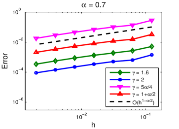
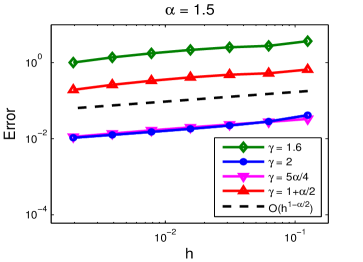
Theorem 3.1 shows that for $u\in C^{1,\frac{\alpha}{2}}({\mathbb{R}}^{2})$, our method has an accuracy of ${\mathcal{O}}(h^{1-\frac{\alpha}{2}})$, independent of the splitting parameter $\gamma$. However, our numerical results indicate that choosing the splitting parameter $\gamma=2$ generally yields smaller numerical errors; see more discussion in Sec. 6.1.

Theorem 3.2.

Suppose that $u\in C^{3,\frac{\alpha}{2}}(\mathbb{R}^{2})$ has finite support on the domain $\Omega\in{\mathbb{R}}^{2}$. Let $(-\Delta)_{\gamma,h}^{\frac{\alpha}{2}}$ be the finite difference approximation of the fractional Laplacian, with $h$ a small mesh size. If the parameter $\gamma=2$, then the local truncation error

$$\big{\|}(-\Delta)^{\frac{\alpha}{2}}u({\bf x})-(-\Delta)^{\frac{\alpha}{2}}_{h,\gamma}u({\bf x})\big{\|}_{\infty}\leq Ch^{2},\qquad\mbox{for}\ \ \alpha\in(0,2)$$ (3.12)

with $C$ a positive constant depending on $\alpha$.

Proof.

Taking $\gamma=2$ in (3.2) and using Lemma 3.1 (ii) with the $\omega(\textit{{\boldmath$\xi$}})=|\textit{{\boldmath$\xi$}}|^{-\alpha}$, we obtain

$$e_{\alpha,2}^{h}({\bf x})=-\frac{c_{2,\alpha}}{4}\bigg{[}\int_{I_{00}}\Big{(}4\psi_{2}(\xi,\eta)-2\big{(}\psi_{2}(\xi_{1},0)+\psi_{2}(0,\eta_{1})\big{)}\Big{)}|\textit{{\boldmath$\xi$}}|^{-\alpha}\,d\xi d\eta$$ (3.13)

$$\hskip 17.07182pt-\frac{1}{2}\sum_{(i,j)\in\varkappa}\int_{I_{ij}}\Big{(}\Theta_{I_{ij}}^{(1,0)}(\xi,\eta)\partial_{2,1}{\psi_{2}}(\xi,\eta)+\Theta_{I_{ij}}^{(0,1)}(\xi,\eta)\partial_{1,2}{\psi_{2}}(\xi,\eta)\Big{)}\,d\xi\,d\eta$$

$$\hskip 17.07182pt+\sum_{(i,j)\in\varkappa}\sum_{n=0,1}\left(-\frac{1}{2}\right)^{n}\bigg{(}\int_{\xi_{i}}^{\xi_{i+1}}\Big{(}\Theta_{I_{ij}}^{(1,n)}(\xi,\eta_{j+1})\partial_{2,n}{\psi_{2}}(\xi,\eta_{j+1})-\Theta_{I_{ij}}^{(1,n)}(\xi,\eta_{j})\partial_{2,n}{\psi_{2}}(\xi,\eta_{j})\Big{)}d\xi$$

$$\hskip 73.97733pt+\int_{\eta_{j}}^{\eta_{j+1}}\Big{(}\Theta_{I_{ij}}^{(n,1)}(\xi_{i+1},\eta)\partial_{n,2}{\psi_{2}}(\xi_{i+1},\eta)-\Theta_{I_{ij}}^{(n,1)}(\xi_{i},\eta)\partial_{n,2}{\psi_{2}}(\xi_{i},\eta)\Big{)}d\eta\bigg{)}$$

$$\hskip 17.07182pt-\sum_{(i,j)\in\varkappa}\sum_{\begin{subarray}{c}m,n=0,1\\ m+n\neq 0\end{subarray}}(-1)^{m+n}\Big{(}\Theta_{I_{ij}}^{(m,n)}(\textit{{\boldmath$\xi$}}_{(i+1)j})\partial_{m,n}\psi_{2}(\textit{{\boldmath$\xi$}}_{(i+1)j})-\Theta_{I_{ij}}^{(m,n)}(\textit{{\boldmath$\xi$}}_{ij})\partial_{m,n}\psi_{2}(\textit{{\boldmath$\xi$}}_{ij})$$

$$\hskip 73.97733pt+\Theta_{I_{ij}}^{(m,n)}(\textit{{\boldmath$\xi$}}_{i(j+1)})\partial_{m,n}\psi_{2}(\textit{{\boldmath$\xi$}}_{i(j+1)})-\Theta_{I_{ij}}^{(m,n)}(\textit{{\boldmath$\xi$}}_{(i+1)(j+1)})\partial_{m,n}\psi_{2}(\textit{{\boldmath$\xi$}}_{(i+1)(j+1)})\Big{)}$$

$$= -\frac{c_{2,\alpha}}{4}\big{(}I+II+III+IV\big{)}.$$

For term $I$, by the triangle inequality and Taylor’s theorem, we get

$$|\,I\,| = \bigg{|}\int_{0}^{h}\int_{0}^{h}\Big{(}4\psi_{2}(\xi,\eta)-2\big{(}\psi_{2}(h,0)+\psi_{2}(0,h)\big{)}\Big{)}|\textit{{\boldmath$\xi$}}|^{-\alpha}d\xi d\eta\,\bigg{|}$$ (3.14)

$$\leq \int_{0}^{h}\int_{0}^{h}\Big{|}4\psi_{2}(\xi,\eta)-2\big{(}\psi_{2}(h,0)+\psi_{2}(0,h)\big{)}\Big{|}|\textit{{\boldmath$\xi$}}|^{-\alpha}d\xi d\eta$$

$$\leq Ch\max_{(\xi,\eta)\in[0,h]^{2}}\Big{\{}\left|\partial_{1,0}\psi_{2}(\xi,\eta)\right|,\left|\partial_{0,1}\psi_{2}(\xi,\eta)\right|\Big{\}}\int_{0}^{h}\int_{0}^{h}|\textit{{\boldmath$\xi$}}|^{-\alpha}d\xi d\eta\,\leq\,Ch^{3-\frac{\alpha}{2}},\qquad$$

where the last inequality is obtained using Lemma 3.3 (ii) and the inequality (3.5).

For term $II$, we first rewrite it as

$$II = -\frac{1}{2}\sum_{(i,j)\in\varkappa}\int_{I_{ij}}\Big{(}\Theta_{I_{ij}}^{(1,0)}(\xi,\eta)\partial_{2,1}{\psi_{2}}(\xi,\eta)+\Theta_{I_{ij}}^{(0,1)}(\xi,\eta)\partial_{1,2}{\psi_{2}}(\xi,\eta)\Big{)}\,d\xi d\eta$$

$$= -\frac{1}{2}\bigg{(}\sum_{(i,j)\in\varkappa}\int_{I_{ji}}\Theta_{I_{ij}}^{(1,0)}(\eta,\xi)\partial_{2,1}{\psi_{2}}(\eta,\xi)\,d\xi d\eta+\sum_{(i,j)\in\varkappa}\int_{I_{ij}}\Theta_{I_{ij}}^{(0,1)}(\xi,\eta)\partial_{1,2}{\psi_{2}}(\xi,\eta)\,d\xi d\eta\bigg{)}$$

$$= \frac{1}{2}\sum_{(i,j)\in\varkappa}\int_{I_{ij}}\Theta_{I_{ij}}^{(0,1)}(\xi,\eta)\big{(}\partial_{2,1}{\psi_{2}}(\eta,\xi)+\partial_{1,2}{\psi_{2}}(\xi,\eta)\big{)}\,d\xi d\eta,$$

where the last line is obtained by switching the position of $i$ and $j$ in the first summation, and using Property 3.1 (i). Then, using the triangle inequality, Property 3.1 (ii), Lemma 3.3 (ii), and the Chebyshev integral inequality, we obtain

$$|\,II\,| \leq \frac{1}{2}\sum_{(i,j)\in\varkappa}\int_{\eta_{j}}^{\eta_{j+1}}\int_{\xi_{i}}^{\xi_{i+1}}\big{|}\Theta_{I_{ij}}^{(0,1)}(\xi,\eta)\big{|}\big{|}\partial_{2,1}{\psi_{2}}(\xi,\eta)+\partial_{1,2}{\psi_{2}}(\eta,\xi)\big{|}d\xi d\eta$$ (3.15)

$$\leq C\sum_{(i,j)\in\varkappa}\bigg{(}h\int_{\eta_{j}}^{\eta_{j+1}}\int_{\xi_{i}}^{\xi_{i+1}}|\textit{{\boldmath$\xi$}}|^{-\alpha}d\xi d\eta\bigg{)}\bigg{(}\int_{\eta_{j}}^{\eta_{j+1}}\int_{\xi_{i}}^{\xi_{i+1}}|\textit{{\boldmath$\xi$}}|^{\frac{\alpha}{2}-2}\,d\xi d\eta\bigg{)}$$

$$\leq Ch^{3}\sum_{(i,j)\in\varkappa}\int_{\eta_{j}}^{\eta_{j+1}}\int_{\xi_{i}}^{\xi_{i+1}}|\textit{{\boldmath$\xi$}}|^{-(2+\frac{\alpha}{2})}d\xi d\eta\,\leq\,Ch^{3-\frac{\alpha}{2}},$$

where the last inequality is obtained by the inequality (3.8).

For term $III$, noticing that $\xi_{i}=\eta_{i}$ and applying Property 3.1 (i) and following the same lines as in obtaining (3.15), we get

$$|\,III\,| = \bigg{|}\sum_{(i,j)\in\varkappa}\sum_{n=0,1}\left(-\frac{1}{2}\right)^{n}\bigg{(}\int_{\xi_{i}}^{\xi_{i+1}}\Theta_{I_{ij}}^{(1,n)}(\xi,\eta_{j+1})\big{(}\partial_{2,n}{\psi_{2}}(\xi,\eta_{j+1})+\partial_{n,2}{\psi_{2}}(\eta_{j+1},\xi)\big{)}\,d\xi$$ (3.16)

$$\hskip 85.35826pt-\int_{\xi_{i}}^{\xi_{i+1}}\Theta_{I_{ij}}^{(1,k)}(\xi,\eta_{j})\big{(}\partial_{2,n}{\psi_{2}}(\xi,\eta_{j})+\partial_{n,2}{\psi_{2}}(\eta_{j},\xi)\big{)}\,d\xi\bigg{)}\bigg{|}$$

$$\leq C\sum_{(i,j)\in\varkappa}\sum_{n=0,1}\bigg{(}h^{1+n}\int_{\eta_{j}}^{\eta_{j+1}}\int_{\xi_{i}}^{\xi_{i+1}}|\textit{{\boldmath$\xi$}}|^{-\alpha}d\xi d\eta\bigg{)}\bigg{(}h^{-1}\int_{\eta_{j}}^{\eta_{j+1}}\int_{\xi_{i}}^{\xi_{i+1}}|\textit{{\boldmath$\xi$}}|^{\frac{\alpha}{2}-1-n}\,d\xi d\eta\bigg{)}$$

$$\leq C\sum_{(i,j)\in\varkappa}\sum_{n=0}^{1}\bigg{(}h^{2+n}\int_{\eta_{j}}^{\eta_{j+1}}\int_{\xi_{i}}^{\xi_{i+1}}|\textit{{\boldmath$\xi$}}|^{-(1+n+\frac{\alpha}{2})}d\xi d\eta\bigg{)}\,\leq\,Ch^{2},$$

by the inequality (3.8), where the estimate of $n=0$ is dominant.

Noticing $\xi_{i}=\eta_{i}$ and using Property 3.1 (i), we can rewrite term $IV$ as

$$IV = \sum_{n=0,1}\frac{(-1)^{1+n}}{1+n}\sum_{\begin{subarray}{c}i,j=1\\ i+j\neq 2\end{subarray}}^{N-1}\Big{(}\Theta_{I_{(i-1)j}}^{(1,n)}(\textit{{\boldmath$\xi$}}_{ij})-\Theta_{I_{ij}}^{(1,n)}(\textit{{\boldmath$\xi$}}_{ij})\Big{)}\big{(}\partial_{1,n}\psi_{2}(\xi_{i},\eta_{j})+\partial_{n,1}\psi_{2}(\eta_{j},\xi_{i})\big{)}$$

$$+\sum_{n=0,1}\frac{(-1)^{1+n}}{1+n}\sum_{\begin{subarray}{c}i,j=1\\ i+j\neq 2\end{subarray}}^{N-1}\Big{(}\Theta_{I_{i(j-1)}}^{(1,n)}(\textit{{\boldmath$\xi$}}_{ij})-\Theta_{I_{(i-1)(j-1)}}^{(1,n)}(\textit{{\boldmath$\xi$}}_{ij})\Big{)}\big{(}\partial_{1,n}\psi_{2}(\xi_{i},\eta_{j})+\partial_{n,1}\psi_{2}(\eta_{j},\xi_{i})\big{)}\bigg{)}$$

$$+\sum_{\begin{subarray}{c}m,n=0,1\\ m+n\neq 0\end{subarray}}(-1)^{m+n}\sum_{i=2}^{N-1}\Big{(}\Theta_{I_{(i-1)0}}^{(m,n)}(\textit{{\boldmath$\xi$}}_{i0})-\Theta_{I_{i0}}^{(m,n)}(\textit{{\boldmath$\xi$}}_{i0})\Big{)}\big{(}\partial_{m,n}\psi_{2}(\xi_{N},\eta_{i})+\partial_{n,m}\psi_{2}(\eta_{i},\xi_{N})\big{)}$$

$$+\sum_{\begin{subarray}{c}m,n=0,1\\ m+n\neq 0\end{subarray}}(-1)^{m+n}\sum_{i=1}^{N-1}\Big{(}\Theta_{I_{(N-1)i}}^{(m,n)}(\textit{{\boldmath$\xi$}}_{Ni})-\Theta_{I_{(N-1)(i-1)}}^{(m,n)}(\textit{{\boldmath$\xi$}}_{Ni})\Big{)}\big{(}\partial_{m,n}\psi_{2}(\xi_{i},\eta_{0})+\partial_{n,m}\psi_{2}(\eta_{0},\xi_{i})\big{)}$$

$$+\sum_{\begin{subarray}{c}m,n=0,1\\ m+n\neq 0\end{subarray}}(-1)^{m+n}\Theta_{I_{(N-1)0}}^{(m,n)}(\textit{{\boldmath$\xi$}}_{N0})\big{(}\partial_{m,n}\psi_{2}(\xi_{N},\eta_{0})+\partial_{n,m}\psi_{2}(\eta_{0},\xi_{N})\big{)}$$

$$-\sum_{\begin{subarray}{c}m,n=0,1\\ m+n\neq 0\end{subarray}}(-1)^{m+n}\Theta_{I_{10}}^{(m,n)}(\textit{{\boldmath$\xi$}}_{10})\big{(}\partial_{m,n}\psi_{2}(\xi_{1},\eta_{0})+\partial_{n,m}\psi_{2}(\eta_{0},\xi_{1})\big{)}$$

$$+\sum_{n=0,1}\frac{(-1)^{1+n}}{1+n}\Theta_{I_{11}}^{(1,n)}(\textit{{\boldmath$\xi$}}_{11})\big{(}\partial_{1,n}\psi_{2}(\xi_{1},\eta_{1})+\partial_{n,1}\psi_{2}(\eta_{1},\xi_{1})\big{)}$$

$$+\sum_{n=0,1}\frac{(-1)^{1+n}}{1+n}\Theta^{(1,n)}_{I_{(N-1)(N-1)}}(\textit{{\boldmath$\xi$}}_{NN})\big{(}\partial_{1,n}\psi_{2}(\eta_{N},\xi_{N})+\partial_{n,1}\psi_{2}(\xi_{N},\eta_{N})\big{)}\bigg{]}\qquad\qquad\qquad\qquad$$

$$= IV_{1}+IV_{2}+IV_{3}+IV_{4}+IV_{5}+IV_{6}+IV_{7}+IV_{8}.$$

For term $IV_{1}$, we first use the triangle inequality and obtain

$$|\,IV_{1}\,| = \bigg{|}\sum_{n=0,1}\frac{(-1)^{1+n}}{1+n}\sum_{\begin{subarray}{c}i,j=1\\ i+j\neq 2\end{subarray}}^{N-1}\Big{(}\Theta_{I_{(i-1)j}}^{(1,n)}(\xi_{i},\eta_{j})-\Theta_{I_{ij}}^{(1,n)}(\xi_{i},\eta_{j})\Big{)}\big{(}\partial_{1,n}\psi_{2}(\xi_{i},\eta_{j})+\partial_{n,1}\psi_{2}(\eta_{j},\xi_{i})\big{)}\bigg{|}$$

$$\leq C\sum_{n=0,1}\sum_{\begin{subarray}{c}i,j=1\\ i+j\neq 2\end{subarray}}^{N-1}\Big{|}\Theta_{I_{(i-1)j}}^{(1,n)}(\xi_{i},\eta_{j})-\Theta_{I_{ij}}^{(1,n)}(\xi_{i},\eta_{j})\Big{|}\big{|}\partial_{1,n}\psi_{2}(\xi_{i},\eta_{j})+\partial_{n,1}\psi_{2}(\eta_{j},\xi_{i})\big{|}$$

To further estimate it, we will need the following property of $\Theta$. Introducing an auxiliary function

$$G^{(1,n)}(x)=\int_{\eta_{j}}^{\eta_{j+1}}\int_{x}^{\xi_{i+1}}|\textit{{\boldmath$\xi$}}|^{-\alpha}(\xi_{i}-{\xi})(\eta_{j}-{\eta})^{n}\,d\xi d\eta,\qquad\mbox{for}\ \ n=0,\mbox{or}\ 1,$$

we can write

$$\Theta_{I_{(i-1)j}}^{(1,n)}(\xi_{i},\eta_{j})-\Theta_{I_{ij}}^{(1,n)}(\xi_{i},\eta_{j})=n!\big{(}G^{(1,n)}(\xi_{i+1})-G^{(1,n)}(\xi_{i-1})\big{)}.$$

Then, we apply Taylor’s theorem to obtain

$$\big{|}G^{(1,n)}(\xi_{i+1})-G^{(1,n)}(\xi_{i-1})\big{|}\leq Ch^{4+n}\Big{(}\sqrt{\xi_{i}^{2}+\eta_{j}^{2}}\Big{)}^{-(1+\alpha)}.$$ (3.17)

By (3.17) and Lemma 3.3 (ii), we then obtain

$$|\,IV_{1}\,| \leq C\sum_{n=0,1}h^{4+n}\sum_{\begin{subarray}{c}i,j=1\\ i+j\neq 2\end{subarray}}^{N-1}\Big{(}\sqrt{\xi_{i}^{2}+\eta_{j}^{2}}\Big{)}^{-(1+n+\frac{\alpha}{2})}\leq\sum_{n=0,1}h^{2+n}\int_{h}^{L}\int_{h}^{L}|\textit{{\boldmath$\xi$}}|^{-(1+n+\frac{\alpha}{2})}\leq Ch^{2}.$$

The estimates of terms $IV_{2}$, $IV_{3}$ and $IV_{4}$ can be done by following the similar lines above, i.e., using (3.17) and Lemma 3.3 (ii). While the estimates of terms $IV_{5}$, $IV_{6}$, $IV_{7}$ and $IV_{8}$ can be done by using Properties 3.1 (ii) and Lemma 3.3 (ii). To avoid redundancy, we will only summarize the results as follows:

$$|\,IV_{2}\,|,|\,IV_{5}\,|,|\,IV_{6}\,|\leq Ch^{2},\qquad|\,IV_{3}\,|,|\,IV_{4}\,|,|\,IV_{7}\,|,|\,IV_{8}\,|\leq Ch^{3-\frac{\alpha}{2}},$$

and thus we have term $IV$,

$$|\,IV\,|\leq\sum_{i=1}^{8}|\,IV_{i}\,|\leq Ch^{2}.$$ (3.18)

Combining (3.13) with (3.14), (3.15), (3.16) and (3.18) yields the estimate (3.12) immediately. ∎

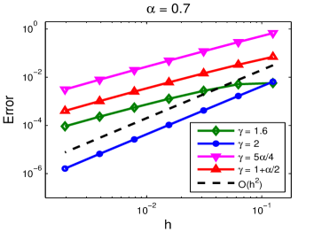
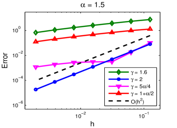
Theorem 3.2 shows that for $u\in C^{3,\frac{\alpha}{2}}({\mathbb{R}}^{2})$, if the splitting parameter is chosen to be optimal, i.e., $\gamma=2$, our method has the second order of accuracy, uniformly for any $\alpha\in(0,2)$.

4 Full discretization and its efficient computations

In this section, we present a numerical method to the fractional reaction-diffusion equation (1.1)–(1.3), study the convergence of its numerical solution to the exact solution, and present a fast algorithm for its efficient computations. Choose a time step $\tau>0$, and define the time sequence $t_{n}=n\tau$, for $n=0,1,\ldots$. Let $u_{ij}^{n}$ be the numerical approximation to the solution $u(x_{i},y_{j},t_{n})$. Using the finite difference method in Sec. 2 for spatial discretization and the Crank–Nicolson for temporal discretization, we obtain the following numerical scheme for the fractional reaction-diffusion equation (1.1):

$$\frac{u^{n+1}_{ij}-u^{n}_{ij}}{\tau}=-\frac{\kappa_{2}}{2}\Big{(}(-\Delta)^{\frac{\alpha}{2}}_{h,\gamma}u^{n}_{ij}+(-\Delta)^{\frac{\alpha}{2}}_{h,\gamma}u^{n+1}_{ij}\Big{)}+\frac{1}{2}\Big{(}f(u^{n}_{ij})+f(u^{n+1}_{ij})\Big{)},\quad$$ (4.1)

for $n=1,\ldots$, and at $t=0$, the initial condition (1.2) is discretized as

$$u_{ij}^{0}=\phi(x_{i},y_{j}),$$ (4.2)

for $1\leq i\leq N_{x}-1$ and $1\leq j\leq N_{y}-1$. Note that the extended Dirichlet boundary conditions have been considered when discretizing the fractional Laplacian $(-\Delta)^{\frac{\alpha}{2}}$. The matrix-vector form of (4.1) is given by

$$\Big{(}{\rm I}+\frac{\kappa_{2}\tau}{2}{\rm A}_{2}\Big{)}{\bf u}^{n+1}=\Big{(}{\rm I}-\frac{\kappa_{2}\tau}{2}{\rm A}_{2}\Big{)}{\bf u}^{n}+\frac{\tau}{2}\Big{(}f({\bf u}^{n})+f({\bf u}^{n+1})\Big{)},\qquad n=0,1,\ldots,$$ (4.3)

with ${\bf u}^{n}$ approximates ${\bf u}(t_{n})$, and the block vector ${\bf u}(t_{n})$ as defined in (2.16). Next, we will perform the convergence analysis of the fully-discretized scheme (4.1)–(4.2).

Theorem 4.1.

Suppose that the solution of the fractional reaction-diffusion equation (1.1)–(1.3) satisfies $u\in C^{2}\big{(}[0,T];C^{s,\frac{\alpha}{2}}({\mathbb{R}}^{2})\big{)}$ with $s\geq 1$, and the reaction term $f(u)$ is Lipschitz continuous. Then, the solution of the finite difference equations (4.1)–(4.2) with $\gamma=2$ convergences to the exact solution of (1.1)–(1.3). Moreover, for $s\geq 3$ the convergence rate is $\mathcal{O}(\tau^{2}+h^{2})$, provided that $h$ and $\tau$ are small enough.

Proof.

Let ${\bf x}_{ij}=(x_{i},y_{j})$. Taking the average of (1.1) at $({\bf x}_{ij},t_{n})$ and $({\bf x}_{ij},t_{n+1})$, we get:

$$\frac{1}{2}\Big{(}\partial_{t}u({\bf x}_{ij},t_{n})+\partial_{t}u({\bf x}_{ij},t_{n+1})\Big{)}=\frac{1}{2}\sum_{l=0,1}\Big{(}-\kappa_{2}(-\Delta)^{\frac{\alpha}{2}}u({\bf x}_{ij},t_{n+l})+f(u({\bf x}_{ij},t_{n+l}))\Big{)}$$ (4.4)

Using Taylor’s theorem at $t=t_{n}$ and $t=t_{n+1}$ on the left-hand side of (4.4) and combining with the spatial error analysis in Theorems 3.1–3.2, it is easy to get

$$\frac{u({\bf x}_{ij},t_{n+1})-u({\bf x}_{ij},t_{n})}{\tau}=\frac{1}{2}\sum_{l=0,1}\Big{(}-\kappa_{2}(-\Delta)_{h,\gamma}^{\frac{\alpha}{2}}u({\bf x}_{ij},t_{n+l})+f\big{(}u({\bf x}_{ij},t_{n+l})\big{)}\Big{)}+\mathcal{O}(\tau^{2}+h^{p}),\ \$$ (4.5)

with $p>0$. Subtracting (4.1) from (4.5) yields

$$\frac{1}{\tau}\big{(}e^{n+1}_{ij}-e^{n}_{ij}\big{)}=-\frac{\kappa_{2}}{2}\Big{(}(-\Delta)_{h,\gamma}^{\frac{\alpha}{2}}\big{(}e^{n}_{ij}+e^{n+1}_{ij}\big{)}\Big{)}+\frac{1}{2}\big{(}\delta f_{ij}^{n}+\delta f_{ij}^{n+1}\big{)}+R,$$ (4.6)

where we denote $e_{ij}^{n}=u({\bf x}_{ij},t_{n})-u_{ij}^{n}$ and $\delta f_{ij}^{n}=f\big{(}u({\bf x}_{ij},t_{n})\big{)}-f\big{(}u_{ij}^{n}\big{)}$, and $R\sim{\mathcal{O}}(\tau^{2}+h^{p})$. Multiplying $\big{(}e^{n+1}_{i,j}+e^{n}_{i,j}\big{)}$ at both sides of (4.6) and summing it over $i,j$, we obtain

$$\|{\bf e}^{n+1}\|_{l_{2}}^{2}-\|{\bf e}^{n}\|_{l_{2}}^{2}\leq\frac{\tau h^{2}}{2}\sum_{i=1}^{N_{x}-1}\sum_{j=1}^{N_{y}-1}\big{(}e_{ij}^{n}+e_{ij}^{n+1}\big{)}\big{(}\delta f_{ij}^{n}+\delta f_{ij}^{n+1}\big{)}+\tau h^{2}|R|\sum_{i=1}^{N_{x}-1}\sum_{j=1}^{N_{y}-1}\big{(}e^{n+1}_{ij}+e^{n}_{ij}\big{)},\ \$$

since the matrix $A_{2}$ from discretizing the 2D fractional Laplacian is positive definite. Using the triangle inequality, and the Lipschitz condition of $f(u)$, we further obtain

$$\|{\bf e}^{n+1}\|_{l_{2}}^{2}-\|{\bf e}^{n}\|_{l_{2}}^{2} \leq \frac{{C}_{0}\tau}{2}\bigg{|}h^{2}\sum_{i=1}^{N_{x}-1}\sum_{j=1}^{N_{y}-1}\big{(}\big{|}e_{ij}^{n}\big{|}+\big{|}e_{ij}^{n+1}\big{|}\big{)}^{2}\bigg{|}+\tau h^{2}|R|\bigg{|}\sum_{i=1}^{N_{x}-1}\sum_{j=1}^{N_{y}-1}\big{(}e^{n+1}_{ij}+e^{n}_{ij}\big{)}\bigg{|}$$ (4.7)

$$\leq \frac{C_{0}\tau}{2}\big{(}\big{\|}{\bf e}^{n+1}\big{\|}_{l^{2}}+\big{\|}{\bf e}^{n}\big{\|}_{l^{2}}\big{)}^{2}+\tau|R|(\|{\bf e}^{n+1}\|_{l_{2}}+\|{\bf e}^{n}\|_{l_{2}}),$$

where $C_{0}$ is the Lipschitz constant of $f$. Dividing $\big{(}\|{\bf e}^{n+1}\|_{l_{2}}+\|{\bf e}^{n}\|_{l_{2}}\big{)}$ at both sides, we then get

$$\|{\bf e}^{n+1}\|_{l_{2}}-\|{\bf e}^{n}\|_{l_{2}}\leq\frac{C_{0}\tau}{2}(\|{\bf e}^{n}\|_{l_{2}}+\|{\bf e}^{n+1}\|_{l_{2}})+\tau\,|R|.$$

Assuming $\tau\leq 1/C_{0}$, we further obtain

$$\|{\bf e}^{n+1}\|_{l_{2}}\,\leq\,\Big{(}1+\frac{C_{0}\tau}{1-C_{0}\tau/2}\Big{)}\|{\bf e}^{n}\|_{l_{2}}+\frac{\tau}{1-C_{0}\tau/2}\,|R|\,\leq\,(1+2C_{0}\tau)\|{\bf e}^{n}\|_{l_{2}}+\frac{C\tau}{1-C_{0}\tau/2}(\tau^{2}+h^{p}).$$

Repeating the above inequality at steps $n,n-1,\ldots 1$, and noticing $\|{\bf e}^{0}\|_{l^{2}}=0$, we get

$$\|{\bf e}^{n+1}\|_{l_{2}} \leq \frac{C\tau}{1-C_{0}\tau/2}(\tau^{2}+h^{p})\sum_{k=0}^{n}(1+2C_{0}\tau)^{k}$$

$$\leq C\big{(}e^{2C_{0}T}-1\big{)}(\tau^{2}+h^{p})\leq C(\tau^{2}+h^{p}),$$

where the constant $C$ is independent of $\tau$ and $h$. Combining the results in Theorems 3.1 and 3.2, we can determine the value of $p$. ∎

In practice, we solve the nonlinear system (4.3) by the fixed point iteration, i.e., letting ${\bf u}^{n+1,0}={\bf u}^{n}$, and at each iteration step $m=0,1,\ldots$, solving

$$\Big{(}{\rm I}+\frac{\kappa_{2}\tau}{2}{A_{2}}\Big{)}{\bf u}^{n+1,m+1}=\Big{(}{\rm I}-\frac{\kappa_{2}\tau}{2}{A_{2}}\Big{)}{\bf u}^{n}+\frac{\tau}{2}\Big{(}f({\bf u}^{n})+f({\bf u}^{n+1,m})\Big{)},$$ (4.8)

for ${\bf u}^{n+1,m+1}$. In our simulations, the iteration is stopped, if $\max|{\bf u}^{n+1,m+1}-{\bf u}^{n+1,m}|<10^{-8}$ is satisfied. At each iteration step $m$, if the Gaussian elimination method is used, the computational cost of solving the linear system (4.8) is of ${\mathcal{O}}(M^{3})$ with $M=(N_{x}-1)(N_{y}-1)$. Here, noticing that the stiffness matrix $({\rm I}+\frac{\kappa_{2}\tau}{2}A_{2})$ is symmetric and positive definite, we propose the conjugate gradient (CG) method to solve the linear system (4.8). At each CG iteration step, we need to evaluate two inner products and one matrix-vector product, and as $A_{2}$ is a large dense matrix, the computational costs of the matrix-vector multiplication are extremely expensive.

Noticing that ${A_{2}}$ is a block-Toeplitz-Toeplitz-block matrix, next we introduce a fast algorithm for the matrix-vector multiplication ${A}_{2}{\bf u}$ for ${\bf u}\in{\mathbb{R}}^{M}$. The main idea is to embed the block-Toeplitz-Toeplitz-block $A_{2}$ matrix into a block-circulant-circulant-block matrix $C$, and then use the fast Fourier transformation (FFT) to compute its matrix-vector products. We will outline the main steps as follows. First, we embed the Toeplitz matrix ${\rm A}_{x,j}$ (for $0\leq j\leq N_{y}-2$) into a double sized circulant matrix and obtain

$${{C}}_{x,j}=\left(\begin{array}[]{cc}{A}_{x,j}&{T}_{x,j}\\ {T}_{x,j}&{A}_{x,j}\end{array}\right)_{2(N_{x}-1)\times 2(N_{x}-1)},$$ (4.11)

for $0\leq j\leq N_{x}-1$, where ${\rm T}_{x,j}$ is a Toeplitz matrix defined by

$${T}_{x,j}:=\left(\begin{array}[]{cccccc}0&a_{(N_{x}-2)j}&\ldots&a_{2j}&a_{1j}\\ a_{(N_{x}-2)j}&0&a_{(N_{x}-2)j}&\cdots&a_{2j}\\ \vdots&\ddots&\ddots&\ddots&\vdots\\ a_{2j}&\ldots&a_{(N_{x}-2)j}&0&a_{(N_{x}-2)j}\\ a_{1j}&a_{2j}&\ldots&a_{(N_{x}-2)j}&0\end{array}\right)_{(N_{x}-1)\times(N_{x}-1)}.$$ (4.17)

From it, we can construct a block-Toeplitz-circulant-block matrix $\bar{C}_{2M\times 2M}$ with the same structure as that in (2.22) but each block is ${C}_{x,j}$.

Second, as ${\bar{C}}$ is also a block Toeplitz matrix, we can further embed ${\bar{C}}$ it into a double sized block circulant matrix and obtain

$${{C}}=\left(\begin{array}[]{cc}{\bar{C}}&{{T}}\\ {{T}}&{\bar{C}}\end{array}\right)_{4M\times 4M},$$ (4.20)

where the matrix $T$ is defined by

$${{T}}=\left(\begin{array}[]{cccccc}0&C_{x,N_{y}-2}&\ldots&C_{x,2}&C_{x,1}\\ C_{x,N_{y}-2}&0&C_{x,N_{y}-2}&\cdots&C_{x,2}\\ \vdots&\ddots&\ddots&\ddots&\vdots\\ C_{x,2}&\ldots&C_{x,N_{y}-2}&0&C_{x,N_{y}-2}\\ C_{x,1}&C_{x,2}&\ldots&C_{x,N_{y}-2}&0\end{array}\right)_{2M\times 2M}.$$ (4.26)

Here, $C$ is a block-circulant-circulant-block matrix, and it can be decomposed as [7]:

$${C}=\big{(}F_{(2N_{y}-2)}\otimes F_{(2N_{x}-2)}\big{)}^{-1}\,\text{diag}(\widehat{{\bf c}})\,\big{(}F_{(2N_{y}-2)}\otimes F_{(2N_{x}-2)}\big{)},$$

where $\big{(}F_{(2N_{y}-2)}\otimes F_{(2N_{x}-2)}\big{)}$ represents the 2D discrete Fourier transform matrix, and $\hat{{\bf c}}=\big{(}F_{(2N_{y}-2)}\otimes F_{(2N_{x}-2)}\big{)}{\bf c}$ with ${\bf c}$ being the first column of matrix ${\rm C}$. Let the vector ${\bf v}_{x,j}=\big{(}{\bf u}_{x,j},\,{\bf 0}_{1\times(N_{x}-1)}\big{)}$, and introduce the block vector ${\bar{\bf v}}=\big{(}{\bf v}_{x,1},\,{\bf v}_{x,2},\,\dots,\,{\bf v}_{x,N_{y}-1}\big{)}_{1\times 2M}$ and ${\bf v}=\big{(}\bar{\bf v},\,{\bf 0}_{1\times 2M}\big{)}^{T}$. Then, the matrix-vector product Cv can be written as

$${\rm C}{\bf v}=\big{(}F_{(2N_{y}-2)}\otimes F_{(2N_{x}-2)}\big{)}^{-1}\big{[}{\text{diag}}\big{(}\big{(}F_{(2N_{y}-2)}\otimes F_{(2N_{x}-2)}\big{)}{\bf c}\big{)}\big{]}\,\big{(}F_{(2N_{y}-2)}\otimes F_{(2N_{x}-2)}\big{)}{\bf v}.$$

In practice, it can be efficiently computed via the 2D fast Fourier transform (FFT2) and its inverse transform. Hence, the computational cost is $\mathcal{O}(M\log M)$, instead of ${\mathcal{O}}(M^{2})$ in a conventional computation of matrix-vector multiplication. Furthermore, the matrix can be stored in $\mathcal{O}(M)$ memory, instead of ${\mathcal{O}}(M^{2})$.

Finally, let ${\bf w}$ be the the first $2M$ entries of the vector ${\rm C}{\bf v}$. Then we can obtain the product $A_{2}{\bf u}$ from ${\bf w}$, by removing every other $N_{x}$ entries of the vector ${\bf w}$. Therefore, the computational complexity of each CG iteration step reduces to $\mathcal{O}(M\log M)$.

Another practice issue is the evaluation of the entries of $A_{2}$, i.e., the coefficients $a_{mn}$ in (2.14)–(2.15). In general, the entries of the stiffness matrix in high-dimensional (i.e., $d\geq 2$) case have to be evaluated numerically. Here, we mainly use the MATLAB built-in function ‘integral2.m’ to compute the double integral of $a_{mn}$ with a tolerance of $10^{-16}$. However, extra treatments should be made in computing $a_{11}$ and the integral over $D_{2}$ in (2.15) to ensure the accuracy. More precisely, for the integral of the form $\int_{p}^{q}\int_{p}^{q}|\textit{{\boldmath$\xi$}}|^{-\beta}d\textit{{\boldmath$\xi$}}$ (for $q>p\geq 0$), when either $p=0$ or $q=\infty$, we first adapt the polar coordinator and write

$$\int_{p}^{q}\int_{p}^{q}|\textit{{\boldmath$\xi$}}|^{-\beta}d\textit{{\boldmath$\xi$}}=2\int_{0}^{\frac{\pi}{4}}\int_{p\csc\theta}^{q\sec\theta}r^{1-\beta}drd\theta=\frac{2}{2-\beta}\int_{0}^{\frac{\pi}{4}}\Big{(}\big{(}q\sec\theta\big{)}^{2-\beta}-\big{(}p\sec\theta\big{)}^{2-\beta}\Big{)}d\theta.$$

Then, it can be computed by the MATLAB built-in function ‘integral.m’. It is easy to see from (2.14) that $a_{mn}=a_{nm}$, for any $m,n\geq 0$. Hence, we only need to evaluate around $(N_{x}-1)(N_{y}-1)/2$ double integrals in the simulations, which can be prepared once and used in all time steps.

5 Generalization to three dimensions

So far, numerical methods for discretizing the 3D hypersingular integral fractional Laplacian (1.4) are still missing in the literature, and thus numerical studies of the corresponding fractional PDEs are limited to 1D and 2D. In this section, we will generalize our study in Sec. 2–3 to present a finite difference scheme for the 3D fractional Laplacian and apply it to solve the problem (1.1)–(1.3). For brevity, we will only outline the main steps and results.

Let the domain $\Omega=(a_{x},b_{x})\times(a_{y},b_{y})\times(a_{z},b_{z})$. Following the same lines as in Sec. 2, we can rewrite the 3D fractional Laplacian (1.4) as a weighted integral, i.e.,

$$(-\Delta)^{\frac{\alpha}{2}}u({\bf x})=-c_{3,\alpha}\int_{0}^{\infty}\int_{0}^{\infty}\int_{0}^{\infty}\psi_{\gamma}({\bf x},\textit{{\boldmath$\xi$}})\omega_{\gamma}(\textit{{\boldmath$\xi$}})\,d\xi d\eta d\zeta,\qquad\mbox{for}\ \ \alpha\in(0,2),$$ (5.1)

where the vector $\xi$$=(\xi,\,\eta,\,\zeta)$ with $\xi=|x-x^{\prime}|$, $\eta=|y-y^{\prime}|$ and $\zeta=|z-z^{\prime}|$. The function

$$\psi_{\gamma}({\bf x},\textit{{\boldmath$\xi$}}):=\frac{1}{|\textit{{\boldmath$\xi$}}|^{\gamma}}\bigg{(}\sum_{m,n,s=0,1}u\big{(}x+(-1)^{m}\xi,\,y+(-1)^{n}\eta,\,z+(-1)^{s}\zeta\big{)}-8u({\bf x})\bigg{)},$$ (5.2)

and the weight function $\omega_{\gamma}(\textit{{\boldmath$\xi$}})=|\textit{{\boldmath$\xi$}}|^{\gamma-(3+\alpha)}$. Choose a constant $\displaystyle L=\max\big{\{}b_{x}-a_{x},\,b_{y}-a_{y},\,b_{z}-a_{z}\big{\}}$. Denote points $\xi_{i}=ih$, $\eta_{j}=jh$, $\zeta_{k}=kh$, for $0\leq i,j,k\leq N$, with the mesh size $h=L/N$. For notational convenience, we let $\textit{{\boldmath$\xi$}}_{ijk}=(\xi_{i},\eta_{j},\zeta_{k})$, and $|\textit{{\boldmath$\xi$}}_{ijk}|=\sqrt{\xi_{i}^{2}+\eta_{j}^{2}+\zeta_{k}^{2}}$,  for $0\leq i,j,k\leq N$. Splitting the integral in (5.1) into two parts, i.e., over $D_{1}=(0,L)^{3}$ and $D_{2}=\big{(}{\mathbb{R}}^{3}_{+}\big{)}\backslash D_{1}$, and noticing $\psi_{\gamma}({\bf x},\textit{{\boldmath$\xi$}})=-8u({\bf x})|\textit{{\boldmath$\xi$}}|^{-\gamma}$, for any $\textit{{\boldmath$\xi$}}\in D_{2}$, we obtain

$$(-\Delta)^{\frac{\alpha}{2}}u({\bf x})=-c_{3,\alpha}\Big{(}\int_{D_{1}}\psi_{\gamma}({\bf x},\textit{{\boldmath$\xi$}})\omega_{\gamma}(\textit{{\boldmath$\xi$}})\,d\textit{{\boldmath$\xi$}}+\int_{D_{2}}\psi_{\gamma}({\bf x},\textit{{\boldmath$\xi$}})\omega_{\gamma}(\textit{{\boldmath$\xi$}})\,d\textit{{\boldmath$\xi$}}\Big{)}$$

$$\hskip 56.9055pt=-c_{3,\alpha}\bigg{(}\sum_{i,j,k=0}^{N-1}\int_{I_{ijk}}\psi_{\gamma}({\bf x},\textit{{\boldmath$\xi$}})\omega_{\gamma}(\textit{{\boldmath$\xi$}})\,d\textit{{\boldmath$\xi$}}-8u({\bf x})\int_{D_{2}}|\textit{{\boldmath$\xi$}}|^{-(3+\alpha)}d\textit{{\boldmath$\xi$}}\bigg{)},\qquad\qquad\quad$$ (5.3)

where the element $I_{ijk}$ is defined as $I_{ijk}:=[ih,\,(i+1)h]\times[jh,\,(j+1)h]\times[kh,\,(k+1)h]$.

We now focus on approximating the integral over each element $I_{ijk}$. If $i+j+k\neq 0$, we apply the weighted trapezoidal rule and obtain:

$$\int_{I_{ijk}}\psi_{\gamma}({\bf x},\textit{{\boldmath$\xi$}})\omega_{\gamma}(\textit{{\boldmath$\xi$}})\,d\textit{{\boldmath$\xi$}}\,\approx\,\frac{1}{8}\bigg{(}\sum_{m,n,s=0,1}\psi_{\gamma}\big{(}{\bf x},\textit{{\boldmath$\xi$}}_{(i+m)(j+n)(k+s)}\big{)}\bigg{)}\int_{I_{ijk}}\omega_{\gamma}(\textit{{\boldmath$\xi$}})\,d\textit{{\boldmath$\xi$}}.$$ (5.4)

If $i=j=k=0$, we get the approximation

$$\int_{I_{000}}\psi_{\gamma}({\bf x},\textit{{\boldmath$\xi$}})\omega_{\gamma}(\textit{{\boldmath$\xi$}})\,d\textit{{\boldmath$\xi$}}\,\approx\,\frac{1}{8}\bigg{(}\lim_{\textit{{\boldmath$\xi$}}\rightarrow{\bf 0}}\psi_{\gamma}({\bf x},\textit{{\boldmath$\xi$}})+\sum_{\begin{subarray}{c}m,n,s=0,1\\ m+n+s\neq 0\end{subarray}}\psi_{\gamma}\big{(}{\bf x},\textit{{\boldmath$\xi$}}_{(i+m)(j+n)(k+s)}\big{)}\bigg{)}\int_{I_{000}}\omega_{\gamma}(\textit{{\boldmath$\xi$}})\,d\textit{{\boldmath$\xi$}}.$$ (5.5)

Assuming the above limit exists, we divide our discussion into two parts: if $\gamma=2$, we obtain:

$$\lim_{\textit{{\boldmath$\xi$}}\rightarrow{\bf 0}}\psi_{2}({\bf x},\textit{{\boldmath$\xi$}})\approx\frac{5}{3}\sum_{\begin{subarray}{c}m,n,s=0,1\\ m+n+s=1\end{subarray}}\psi_{2}\big{(}{\bf x},\textit{{\boldmath$\xi$}}_{mns}\big{)}-\sum_{\begin{subarray}{c}m,n,s=0,1\\ m+n+s>1\end{subarray}}\psi_{2}\big{(}{\bf x},\textit{{\boldmath$\xi$}}_{mns}\big{)},\quad\ \ \mbox{if}\ \ \gamma=2.$$ (5.6)

while if $\gamma\in(\alpha,2)$, we get

$$\lim_{\textit{{\boldmath$\xi$}}\rightarrow{\bf 0}}\psi_{\gamma}({\bf x},\textit{{\boldmath$\xi$}})=\lim_{\textit{{\boldmath$\xi$}}\rightarrow{\bf 0}}\Big{(}\psi_{2}({\bf x},\textit{{\boldmath$\xi$}})\,|\textit{{\boldmath$\xi$}}|^{2-\gamma}\Big{)}=0,\quad\ \ \text{for}\ \ \gamma\in(\alpha,\,2),$$ (5.7)

Substituting (5.6)–(5.7) into (5.5), we obtain the approximation of the integral over $I_{000}$ as:

$$\int_{I_{000}}\psi_{\gamma}({\bf x},\textit{{\boldmath$\xi$}})\omega(\textit{{\boldmath$\xi$}})\,d\textit{{\boldmath$\xi$}}\approx\frac{1}{8}\bigg{(}\sum_{\begin{subarray}{c}m,n,s=0,1\\ m+n+s\neq 0\end{subarray}}c_{mns}^{\gamma}\psi_{\gamma}\big{(}{\bf x},\textit{{\boldmath$\xi$}}_{mns}\big{)}\bigg{)}\int_{I_{000}}\omega_{\gamma}(\textit{{\boldmath$\xi$}})\,d\textit{{\boldmath$\xi$}},$$ (5.8)

where the coefficient

$$c_{mns}^{\gamma}=\left\{\begin{array}[]{ll}1,&\mbox{if $\gamma\in(\alpha,2)$},\\ 8/3,&\mbox{if $\gamma=2$, and $m+n+s=1$,}\\ 0,&\mbox{if $\gamma=2$, and $m+n+s>1$.}\end{array}\right.$$

Combining (5.3) with (5.4) and (5.8), we obtain

$$(-\Delta)^{\frac{\alpha}{2}}_{h,\gamma}u({\bf x})=-\frac{c_{3,\alpha}}{8}\bigg{[}\sum_{\begin{subarray}{c}i,j,k=0\\ i+j+k\neq 0\end{subarray}}^{N-1}\bigg{(}\sum_{m,n,s=0,1}\psi_{\gamma}\big{(}{\bf x},\textit{{\boldmath$\xi$}}_{(i+m)(j+n)(k+s)}\big{)}\bigg{)}\int_{I_{ijk}}\omega_{\gamma}(\textit{{\boldmath$\xi$}})d\textit{{\boldmath$\xi$}}$$

$$\hskip 79.6678pt+\bigg{(}\sum_{\begin{subarray}{c}m,n,s=0,1\\ m+n+s\neq 0\end{subarray}}\kappa_{mns}^{\gamma}\psi_{\gamma}\big{(}{\bf x},\textit{{\boldmath$\xi$}}_{mns}\big{)}\bigg{)}\int_{I_{000}}\omega_{\gamma}(\textit{{\boldmath$\xi$}})d\textit{{\boldmath$\xi$}}-64\,u({\bf x})\int_{D_{2}}|\textit{{\boldmath$\xi$}}|^{-(3+\alpha)}d\textit{{\boldmath$\xi$}}\bigg{)}.\qquad\qquad$$ (5.10)

Without loss of generality, we assume that $N_{x}=N$, and choose $N_{y},N_{z}$ as the smaller integer such that $a_{y}+N_{y}h\geq b_{y}$ and $a_{z}+N_{z}h\geq b_{z}$. Define the grid points $x_{i}=a_{x}+ih$ for $0\leq i\leq N_{x}$, $y_{j}=a_{y}+jh$ for $0\leq j\leq N_{y}$, and $z_{k}=a_{z}+kh$ for $0\leq k\leq N_{z}$. Let $u_{ijk}$ represent the solution $u(x_{i},y_{j},z_{k})$. Combining (5) with (5.2) and simplifying the calculations, we then obtain

$$(-\Delta)_{h,\gamma}^{\frac{\alpha}{2}}u_{ijk}=-c_{3,\alpha}\bigg{[}a_{000}\,u_{ijk}+\sum_{p=0,1}\bigg{(}\sum_{m\in S_{i}^{p}}a_{m00}\,u_{[i+(-1)^{p}m]jk}+\sum_{n\in S_{j}^{p}}a_{0n0}u_{i[j+(-1)^{p}n]k}$$

$$\hskip 45.52458pt+\sum_{s\in S_{k}^{p}}a_{00s}u_{ij[k+(-1)^{p}s]}\bigg{)}+\sum_{p,q=0,1}\bigg{(}\sum_{s\in S_{k}^{q}}\sum_{n\in S_{j}^{p}}a_{0ns}u_{i[j+(-1)^{p}n][k+(-1)^{q}s]}$$

$$\hskip 45.52458pt+\sum_{s\in S_{k}^{q}}\sum_{m\in S_{i}^{p}}a_{m0s}u_{[i+(-1)^{p}m]j[k+(-1)^{q}s]}+\sum_{n\in S_{j}^{q}}\sum_{m\in S_{i}^{p}}a_{mn0}u_{[i+(-1)^{p}m][j+(-1)^{q}n]\,k}\bigg{)}$$

$$\hskip 45.52458pt+\sum_{p,q,r=0}^{1}\sum_{s\in S_{k}^{r}}\sum_{n\in S_{j}^{q}}\sum_{m\in S_{i}^{p}}a_{mns}u_{[i+(-1)^{p}m][j+(-1)^{q}n][k+(-1)^{r}s]}\bigg{]},$$ (5.11)

for $1\leq i\leq N_{x}-1$, $1\leq j\leq N_{y}-1$, and $1\leq k\leq N_{z}-1$, where the index sets

$$S_{i}^{p}=\big{\{}l\,|\,l\in{\mathbb{N}},\ 1\leq i+(-1)^{p}l\leq N_{x}-1\big{\}},$$

$$S_{j}^{p}=\big{\{}l\,|\,l\in{\mathbb{N}},\ 1\leq j+(-1)^{p}l\leq N_{y}-1\big{\}},$$

$$S_{k}^{p}=\big{\{}l\,|\,l\in{\mathbb{N}},\ 1\leq k+(-1)^{p}l\leq N_{z}-1\big{\}},\qquad p=0,\,\mbox{or}\ 1.$$

Similarly, the coefficients $a_{mns}$ depend on the splitting parameter $\gamma$. For $m+n+s>0$, there is

$$a_{mns}=\frac{2^{\sigma(m,n,s)}}{8|\textit{{\boldmath$\xi$}}_{mns}|^{\gamma}}\bigg{(}\int_{T_{mns}}|\textit{{\boldmath$\xi$}}|^{\gamma-(3+\alpha)}\,d\textit{{\boldmath$\xi$}}-\bar{c}_{mns}\left\lfloor\frac{\gamma}{2}\right\rfloor\int_{I_{000}\cap T_{mns}}|\textit{{\boldmath$\xi$}}|^{\gamma-(3+\alpha)}\,d\textit{{\boldmath$\xi$}}\bigg{)},$$

where $\sigma(m,n,s)$ denotes the number zeros of $m,n$ and $s$, and the constant $\bar{c}_{mns}=-\frac{5}{3}$ if $\sigma(m,n,s)=2$; otherwise, $\bar{c}_{mns}=1$ if $\sigma(m,n,s)<2$. For $0\leq m,n,s\leq N-1$, we denote

$$T_{mns}=\big{(}[(m-1)h,\,(m+1)h]\times[(n-1)h,\,(n+1)h]\times[(s-1)h,\,(s+1)h]\big{)}\cap D_{1},$$

i.e., all the elements associated to the point $\textit{{\boldmath$\xi$}}_{mns}$. The coefficient $a_{000}$ is computed by:

$$a_{000}=-2\sum_{m=1}^{N}\big{(}a_{m00}+a_{0m0}+a_{00m}\big{)}-4\sum_{m,n=1}^{N}\big{(}a_{0mn}+a_{m0n}+a_{mn0}\big{)}$$

$$\hskip 34.14322pt-8\sum_{m,n,s=1}^{N}a_{mns}-8\int_{D_{2}}|\textit{{\boldmath$\xi$}}|^{\gamma-(3+\alpha)}\,d\textit{{\boldmath$\xi$}}.$$

Remark 5.1.

Similar to 2D cases, the optimal splitting parameter is $\gamma=2$. Moreover, as $\alpha\to 2^{-}$, the finite difference scheme in (5) with $\gamma=2$ can reduce to the central difference scheme of the classical 3D Laplace operator $-\Delta$, which can be proved by noticing the facts:

$$\lim_{\alpha\rightarrow 2^{-}}c_{3,\alpha}=0,\qquad\mbox{and}\qquad\lim_{\alpha\rightarrow 2^{-}}\bigg{(}\frac{4c_{3,\alpha}}{3}\int_{I_{000}}\,|\textit{{\boldmath$\xi$}}|^{-(1+\alpha)}\,d\textit{{\boldmath$\xi$}}\bigg{)}=1.$$

Following the similar arguments in proving Theorems 3.1 and 3.2, we can obtain the following estimates on the local truncation errors of the finite difference scheme (5) to the 3D fractional Laplacian $(-\Delta)^{\frac{\alpha}{2}}$. For brevity, we will omit their proofs, which can be done straightforwardly by following lines in proving Theorems 3.1 and 3.2.

Theorem 5.1.

Suppose that $u\in C^{1,\frac{\alpha}{2}}(\mathbb{R}^{3})$ has finite support on the domain $\Omega\in{\mathbb{R}}^{3}$. Let $(-\Delta)_{\gamma,h}^{\frac{\alpha}{2}}$ be the finite difference approximation of the fractional Laplacian $(-\Delta)^{\frac{\alpha}{2}}$. For any $\gamma\in(\alpha,2]$ and $\alpha\in(0,2)$, the local truncation error of $(-\Delta)_{\gamma,h}^{\frac{\alpha}{2}}$ is of ${\mathcal{O}}(h^{1-\frac{\alpha}{2}})$, with $h$ a small mesh size.

Theorem 5.2.

Suppose that $u\in C^{3,\frac{\alpha}{2}}(\mathbb{R}^{3})$ has finite support on the domain $\Omega\in{\mathbb{R}}^{3}$. Let $(-\Delta)_{\gamma,h}^{\frac{\alpha}{2}}$ be the finite difference approximation of the fractional Laplacian $(-\Delta)^{\frac{\alpha}{2}}$. If $\gamma=2$, the local truncation error of $(-\Delta)_{\gamma,h}^{\frac{\alpha}{2}}$ is of ${\mathcal{O}}(h^{2})$ uniformly for any $\alpha\in(0,2)$, with $h$ a small mesh size.

Denote the vector ${\bf u}(t)=\big{(}{\bf u}_{x,y,1}(t),\,\ldots,\,{\bf u}_{x,y,N_{z}-1}(t)\big{)}^{T}$. Here, the block vector ${\bf u}_{x,y,k}(t)=\big{(}{\bf u}_{x,1,k}(t),\,\ldots,\,{\bf u}_{x,N_{y}-1,k}(t)\big{)}$, with each block ${\bf u}_{x,j,k}(t)=\big{(}{u}_{1jk}(t),\,\ldots,\,u_{(N_{x}-1)jk}(t)\big{)}$. Then, the semi-discretization of the fractional reaction-diffusion equation (1.1)–(1.2) reads:

$$\frac{d{\bf u}(t)}{dt}={A_{3}}{\bf u}(t)+f({\bf u}(t)),\qquad t>0.$$ (5.12)

Here, $A_{3}$ is the matrix representation of the 3D fractional Laplacian, defined as:

$${{\rm{A}_{3}}}=\left(\begin{array}[]{cccccc}A_{x,y,0}&A_{x,y,1}&\ldots&A_{x,y,N_{z}-3}&A_{x,y,N_{z}-2}\\ A_{x,y,1}&A_{x,y,0}&A_{x,y,1}&\cdots&A_{x,y,N_{z}-3}\\ \vdots&\ddots&\ddots&\ddots&\vdots\\ A_{x,y,N_{z}-3}&\ldots&A_{x,y,1}&A_{x,y,0}&A_{x,y,1}\\ A_{x,y,N_{z}2}&A_{x,y,N_{z}-3}&\ldots&A_{x,y,1}&A_{x,y,0}\end{array}\right),$$ (5.18)

where for $k=0,1,\dots,N_{z}-2$, the block matrix

$${\rm{A}}_{x,y,k}=\left(\begin{array}[]{cccccc}A_{x,0,k}&A_{x,1,k}&\ldots&A_{x,N_{y}-3,k}&A_{x,N_{y}-2,k}\\ A_{x,1,k}&A_{x,0,k}&A_{x,1,k}&\cdots&A_{x,N_{y}-3,k}\\ \vdots&\ddots&\ddots&\ddots&\vdots\\ A_{x,N_{y}-3,k}&\ldots&A_{x,1,k}&A_{x,0,k}&A_{x,1,k}\\ A_{x,N_{y}-2,k}&A_{x,N_{2}-3,k}&\ldots&A_{x,1,k}&A_{x,0,k}\end{array}\right),$$

with

$${\rm{A}}_{x,j,k}=\left(\begin{array}[]{cccccc}a_{0jk}&a_{1jk}&\ldots&a_{(N_{x}-3)jk}&a_{(N_{x}-2)jk}\\ a_{1jk}&a_{0jk}&a_{1jk}&\cdots&a_{(N_{x}-3)jk}\\ \vdots&\ddots&\ddots&\ddots&\vdots\\ a_{(N_{x}-3)jk}&\ldots&a_{1jk}&a_{0jk}&a_{1jk}\\ a_{(N_{x}-2)jk}&a_{(N_{x}-3)jk}&\ldots&a_{1jk}&a_{0jk}\end{array}\right),$$ (5.25)

for $j=0,1,\dots,N_{y}-2$, and $k=0,1,\dots,N_{z}-2$. Similar to the 2D case, we discretize (5.12) by the Crank–Nicolson method. Note that ${A}_{3}$ is a positive definite matrix. We can obtain the similar conclusions as that in Theorem 4.1. In practice, the resulting system of difference equations are computed by combining the fixed point iteration and the CG method, where the matrix product can be efficiently computed by the 3D FFT. Hence, the computational cost of each CG iteration is of ${\mathcal{O}}(M\log M)$, and the memory cost is ${\mathcal{O}}(M)$, with $M=(N_{x}-1)(N_{y}-1)(N_{z}-1)$.

6 Numerical experiments

In this section, we will first test the numerical accuracy of the finite difference method in discretizing the 2D and 3D fractional Laplacian and compare them with our theoretical results. We remark that our focus here is the spatial accuracy, since the temporal accuracy of the Crank–Nicolson method has been well studied. To test its performance, we then apply our method to solve various fractional reaction-diffusion equations, including the 2D fractional Allen–Cahn equation, and the 2D and 3D fractional Gray–Scott equations.

6.1 Numerical accuracy

Example 1 (2D accuracy).  Consider the function

$$u(x,y)=\left\{\begin{array}[]{ll}\big{(}(1-x^{2})(1-y^{2})\big{)}^{s+\frac{\alpha}{2}},&\text{if}\ \ (x,y)\in\Omega,\\ 0,&\text{otherwise},\end{array}\right.$$ (6.3)

which is in $C^{s,\frac{\alpha}{2}}(\mathbb{R}^{2})$ (for $s\in{\mathbb{N}}$) and has compact support on $\Omega=(-1,1)^{2}$. We use the solution with a fine mesh size $h=1/4096$ as the reference solution in computing numerical errors.

In Tables 1 and 2, we present the numerical errors $\|(-\Delta)^{\frac{\alpha}{2}}{\bf u}-(-\Delta)^{\frac{\alpha}{2}}_{\gamma,h}{\bf u}\|_{\infty}$ and the convergence rates, for the function $u$ in (6.3) with $s=1$ and $3$, respectively, where $\gamma=2$ is used in our method.

	1/16	1/32	1/64	1/128	1/256	1/512
$0.2$	8.312E-4	4.584E-4	2.488E-4	1.340E-4	7.178E-5	3.805E-5
	c.r.	0.8586	0.8817	0.8927	0.9004	0.9158
$0.7$	6.339E-4	5.039E-4	3.415E-4	2.219E-4	1.421E-4	8.998E-5
	c.r.	0.3313	0.5611	0.6222	0.6429	0.6591
$1$	4.087E-3	2.609E-3	1.783E-3	1.246E-3	8.775E-4	6.225E-4
	c.r.	0.6474	0.5496	0.5173	0.5053	0.4953
$1.5$	2.825E-2	2.215E-2	1.818E-2	1.514E-2	1.267E-2	1.061E-2
	c.r.	0.3512	0.2852	0.2640	0.2566	0.2556
$1.9$	3.123E-2	2.504E-2	2.273E-2	2.148E-2	2.055E-2	1.969E-2
	c.r.	0.3188	0.1396	0.0815	0.0636	0.0621

Table 1: Numerical errors $\|(-\Delta)^{\frac{\alpha}{2}}{\bf u}-(-\Delta)^{\frac{\alpha}{2}}_{\gamma,h}{\bf u}\|_{\infty}$ and convergence rates (c.r.), for $u\in C^{1,\frac{\alpha}{2}}({\mathbb{R}}^{2})$ in (6.3), where $\gamma=2$.

For a fixed mesh size $h$, the larger the power $\alpha$, the bigger the numerical errors. Table 1 shows that for $u\in C^{1,\frac{\alpha}{2}}({\mathbb{R}^{2}})$, the accuracy of ${\mathcal{O}}\big{(}h^{1-\frac{\alpha}{2}}\big{)}$, confirming our theoretical results in Theorem 3.1.

	1/16	1/32	1/64	1/128	1/256	1/512
$0.2$	1.062E-4	2.679E-5	6.716E-6	1.679E-6	4.187E-7	1.034E-7
	c.r.	1.9852	1.9959	1.9998	2.0039	2.0170
$0.7$	1.657E-3	4.178E-4	1.048E-4	2.620E-5	6.535E-6	1.615E-6
	c.r.	1.9882	1.9956	1.9992	2.0035	2.0168
$1$	4.594E-3	1.154E-3	2.892E-4	7.231E-5	1.803E-5	4.457E-6
	c.r.	1.9928	1.9970	1.9995	2.0035	2.0167
$1.5$	1.995E-2	4.925E-3	1.219E-3	3.025E-4	7.502E-5	1.847E-5
	c.r.	2.0182	2.0140	2.0111	2.0114	2.0222
$1.9$	6.695E-2	1.653E-2	4.383E-3	1.176E-3	3.011E-4	7.489E-5
	c.r.	2.0183	1.9146	1.8983	1.9654	2.0075

Table 2: Numerical errors $\|(-\Delta)^{\frac{\alpha}{2}}{\bf u}-(-\Delta)^{\frac{\alpha}{2}}_{\gamma,h}{\bf u}\|_{\infty}$ and convergence rates (c.r.) for $u\in C^{3,\frac{\alpha}{2}}({\mathbb{R}}^{2})$ in (6.3), where $\gamma=2$.

Table 2 shows that the accuracy is improved to ${\mathcal{O}}(h^{2})$, uniformly for any $\alpha\in(0,2)$, if the function $u\in C^{3,\frac{\alpha}{2}}({\mathbb{R}}^{2})$, verifying the conclusion in Theorem 3.2.

To further understand the role of $\gamma$, we study the numerical errors for various splitting parameter $\gamma\in(\alpha,2]$ in Figure 1. It shows that for fixed $\alpha$ and $h$, the larger the parameter $\gamma$, the smaller the numerical error. For $u\in C^{1,\frac{\alpha}{2}}({\mathbb{R}}^{2})$, even though different choice of $\gamma$ leads to the same convergence rate ${\mathcal{O}}(h^{1-\frac{\alpha}{2}})$, the numerical errors from $\gamma=2$ are much smaller.

Figure 1: Numerical errors $\|(-\Delta)^{\frac{\alpha}{2}}{\bf u}-(-\Delta)^{\frac{\alpha}{2}}_{\gamma,h}{\bf u}\|_{\infty}$ for different splitting parameter $\gamma\in(\alpha,2]$, where $u$ is defined in (6.3) with $s=1$ (upper row), or $s=3$ (lower row).

By contrast, for $u\in C^{3,\frac{\alpha}{2}}({\mathbb{R}}^{2})$ only the splitting parameter $\gamma=2$ yields the optimal convergence rate ${\mathcal{O}}(h^{2})$, while for $\gamma\in(\alpha,2)$ the method has a lower accuracy, i.e., ${\mathcal{O}}(h^{2-\alpha})$ (see Fig. 1 lower row). Hence, we conclude that $\gamma=2$ is the optimal splitting parameter of high-dimensional finite difference method, distinguishing from the one-dimensional case where both $\gamma=2$ and $\gamma=1+\alpha/2$ are the optimal choices [10].

Example 2 (3D accuracy). Similarly, we consider a function $u\in C^{s,\frac{\alpha}{2}}(\mathbb{R}^{3})$ of the form

$$u(x,y,z)=\left\{\begin{array}[]{ll}\big{(}(1-x^{2})(1-y^{2})(1-z^{2})\big{)}^{s+\frac{\alpha}{2}},&\text{if}\ \ (x,y,z)\in\Omega,\\ 0,&\text{otherwise},\end{array}\right.$$ (6.6)

for $s\in{\mathbb{N}}$. It has compact support on $\Omega=(-1,1)^{3}$. Our extensive simulations show that the splitting parameter $\gamma=2$ is also the optimal choice for the 3D finite difference method proposed in Sec. 5. Hence, we will focus on only the case of $\gamma=2$. Figure 2 shows the numerical errors $\|(-\Delta)^{\frac{\alpha}{2}}{\bf u}-(-\Delta)_{\gamma,h}^{\frac{\alpha}{2}}{\bf u}\|_{\infty}$ for $u\in C^{3,\frac{\alpha}{2}}({\mathbb{R}}^{3})$ in (6.6).

Figure 2: Numerical errors $\|(-\Delta)^{\frac{\alpha}{2}}{\bf u}-(-\Delta)^{\frac{\alpha}{2}}_{\gamma,h}{\bf u}\|_{\infty}$ with $\gamma=2$, for $u\in C^{3,\frac{\alpha}{2}}({\mathbb{R}}^{3})$ in (6.6).

It shows that for a fixed mesh size $h$, the larger the power $\alpha$, the bigger the numerical errors. The numerical results in Fig. 2 agree with our theoretical results in Theorem 5.2 – the accuracy of our method is ${\mathcal{O}}(h^{2})$ for $u\in C^{3,\frac{\alpha}{2}}({\mathbb{R}}^{3})$.

6.2 Fractional Allen–Cahn equation

The Allen–Cahn equation has been widely used in modeling phase field problems arising in materials science and fluid dynamics. Recently, the fractional analogue of the Allen–Cahn equation was proposed to study phase transition in the presence of anomalous diffusion [26]. Here, we apply our method to study the benchmark problem – coalescence of two “kissing” bubbles – in the phase field models. Consider the 2D fractional Allen–Cahn equation [26]:

$$\partial_{t}u({\bf x},t)=-(-\Delta)^{\frac{\alpha}{2}}u-\frac{1}{\varepsilon^{2}}\,u(u^{2}-1),\qquad{\bf x}\in\Omega,\quad t>0,\qquad\qquad$$ (6.7)

$$u({\bf x},t)=-1,\qquad{\bf x}\in\Omega^{c},\quad t\geq 0,$$ (6.8)

where the domain $\Omega=(0,1)^{2}$, and $u$ is the phase field function. The constant $\varepsilon>0$ describes the diffuse interface width. In the following, we take $\varepsilon=0.03$. The initial condition is chosen as

$$u({\bf x},0)=1-\tanh\bigg{(}\frac{d_{1}(x,y)}{2\varepsilon}\bigg{)}-\tanh\bigg{(}\frac{d_{2}(x,y)}{2\varepsilon}\bigg{)},\qquad{\bf x}\in{\mathbb{R}}^{2},$$

with the function $d_{i}(x,y)=\sqrt{(x-x_{i})^{2}+(y-y_{i})^{2}}-0.1$ with $x_{1}=y_{1}=0.4$ and $x_{2}=y_{2}=0.6$. Initially, two bubbles, centered at $(0.4,0.4)$ and $(0.6,0.6)$, respectively, are osculating or “kissing”. In our simulations, we choose the mesh size $h=1/1024$ and the time step $\tau=0.0005$. Note that the boundary condition in (6.8) is nonzero constant. Letting $\bar{u}=u+1$, we can rewrite the problem (6.7) as an equation of $\bar{u}$ with the extended homogeneous boundary conditions as in (1.2).

Figure 3: Dynamics of the two “kissing” bubbles in the classical Allen–Cahn equation (top row) and its fractional counterparts with $\alpha=1.9$ (second row), $1.5$ (third row), and $1.2$ (last row).

Figure 3 shows the time evolution of the two bubbles in both classical (non-fractional) and fractional Allen–Cahn equations. In the classical case, the two bubbles first coalesce into one bubble, and then this newly formed bubble shrinks and are eventually absorbed by the fluid (see Fig. 3 top row). By contrast, their dynamics in the fractional cases crucially depend on $\alpha$. For relative large $\alpha$ (e.g., $\alpha=1.9$ or $1.5$), they evolve similarly to the classical cases, but the process is much slower. Moreover, the smaller the fractional power $\alpha$, the slower the evolution, and consequently it takes a much longer time for the bubbles to vanish for smaller $\alpha$ (cf. $\alpha=1.5$ and $1.9$). When further reducing $\alpha$ (e.g., $\alpha=1.2$), the kissing bubbles separate into two single bubbles and finally vanish at the same time. Fig. 3 also suggests that the width of the interface depends not only on the value of $\varepsilon$ but also on the fractional power $\alpha$: for a fixed $\varepsilon$, the smaller the value of $\alpha$, the thinner the interface. Hence, high spatial resolution is demanded in order to capture the evolution of the interface, implying that the computation of the fractional Allen–Cahn equation is more challenging than its classical counterpart.

6.3 Fractional Gray–Scott equations

The Gray–Scott system was originally proposed for modeling autocatalytic reacting system, and has been well used to study the pattern formation and morphogenesis [19, 23]. In this section, we numerically explore the morphogenesis phenomena in the fractional Gray-Scott equations in two and three dimensions. Consider the fractional Gray–Scott equation:

$$\partial_{t}u({\bf x},t)=-\kappa_{1}(-\Delta)^{\frac{\alpha}{2}}u-uv^{2}+a(1-u),$$ (6.9)

$$\partial_{t}v({\bf x},t)=-\kappa_{2}(-\Delta)^{\frac{\alpha}{2}}v+uv^{2}-(a+b)v,\qquad{\bf x}\in\Omega,\quad t>0,$$ (6.10)

for the concentration of $u$ and $v$, where $\kappa_{1}$ and $\kappa_{2}$ are diffusion coefficients, $a$ is the feed rate, and $b$ is the depletion rate. The system (6.9)–(6.10) admits a trivial solution: $(u,v)\equiv(1,0)$. Let the domain $\Omega=(0,2.5)^{d}$ (for $d=2$ or $3$). The initial condition is chosen as the trivial solution $(u,v)=(1,0)$ with a perturbation at the center of the domain, i.e., $(u,v)=(0.5,0.25)$ for ${\bf x}\in[1.225,1.275]^{2}$ in 2D and ${\bf x}\in[1.15,1.35]^{3}$ in 3D. The boundary conditions of (6.9)–(6.10) are set as

$$u({\bf x},t)=1,\qquad v({\bf x},t)=0,\qquad{\bf x}\in\Omega^{c},\quad t\geq 0.$$

Similar to the situation in Sec. 6.2, we rewrite (6.9)–(6.10) (i.e., changing variable $\bar{u}=u-1$) into a problem with the homogeneous Dirichlet boundary conditions. In our simulations, we choose $\kappa_{1}=2\times 10^{-5}$, $\kappa_{2}=10^{-5}$, and $b=0.065$, the mesh size $h=2.5/1024$, and time step $\tau=0.5$.

Figures 4 and 5 illustrate the pattern formation in the 2D Gray–Scott equation with $a=0.44$ and $0.4$, respectively.

Figure 4: Pattern formation of the component $u$ in the 2D fractional Gray–Scott equation where $a=0.044$. From top to bottom: classical case, fractional cases with $\alpha=1.95,1.8$ and $1.5$.

For easy comparison, we also present the results of the classical Gray–Scott equation. It shows that the pattern starts to develop from the initial perturbation area. In Fig. 4 for $a=0.44$, a mixed pattern of stripes and spots are observed in the classical system (also referred to as pattern $\eta$ in [23]). By contrast, only stripe patterns are observed in the fractional cases. For $\alpha=1.95$, each stripe first grows outwards with a velocity normal to the stripe and then grows inwards after reaching the boundary, until the steady state is formed. The decrease of the fractional power $\alpha$ leads to a much finer structure. For example, for $\alpha=1.5$, a new process of pattern nucleation is observed, and they grow gradually outwards until the entire domain reaches the steady state configuration.

Figure 5: Pattern formation of component $u$ in the 2D fractional Gray–Scott equation where $a=0.04$. From top to bottom: classical case, fractional cases with $\alpha=1.95,1.8$ and $1.5$.

Comparing Figs. 4 and 5, we find that a slight change in parameters could lead to dramatically different patterns. In Fig. 5 for $a=0.4$, a spot configuration is observed in the classical system (also referred to as pattern $\lambda$ in [23]). Although the similar configuration is observed for $\alpha=1.95$, the final pattern is much finer. In contrast to it, a mixed pattern of stripes and spots is formed for $\alpha=1.8$ and $1.5$.

To further demonstrate the effectiveness of our method, we use it to study the pattern formation in the 3D Gray–Scott equations. Note that due to the lack of effective numerical methods, so far no numerical results can be found in the literature on the fractional PDEs with the 3D hypersingular integral fractional Laplacian (1.4). Figure 6 shows the isosurface plots of the component $u$ at different time $t$, where $\alpha=1.9$ and $a=0.4$. For a better resolution, only the region of $[0.9,1.6]^{3}$ is displayed.

Figure 6: Isosurface plots of $u=-0.5$ in the 3D fractional Gray–Scott equation with $\alpha=1.9$.

It shows that the 3D fractional Gray-Scott model exhibits more exotic patterns than the 2D cases. In addition, the computations of the 3D systems become more challenging, however, our method and fast algorithms can ensure both the accuracy and efficiency of the simulations.

7 Conclusions

We proposed an accurate finite difference method to discretize the two and three dimensional fractional Laplacian in hypersingular integral form, applied it to solve the fractional reaction-diffusion equations, and developed a fast algorithm for its efficient computations. The key idea of our method is that we reformulate the fractional Laplacian as the weighted integral of a central difference quotient, so as to avoid directly discretizing the hypersingular integral. The detailed error estimates were provided to understand the accuracy of our method. For $u\in C^{1,\frac{\alpha}{2}}({\mathbb{R}}^{d})$, we proved that our method has an accuracy of ${\mathcal{O}}(h^{1-\frac{\alpha}{2}})$, for any splitting parameter $\gamma\in(\alpha,2]$. Furthermore, our numerical studies showed that although different choices of $\gamma$ leads to the same convergence rate, numerical errors are usually smaller by choosing $\gamma=2$. For $u\in C^{3,\frac{\alpha}{2}}({\mathbb{R}}^{d})$, we proved that our method with $\gamma=2$ has an accuracy of ${\mathcal{O}}(h^{2})$, independent of the power $\alpha\in(0,2)$. Extensive numerical examples were presented to verify our theoretical results. Noticing that our method results in a symmetric block Toeplitz matrix, we thus developed a fast algorithm via fast Fourier transform (FFT) to efficiently compute the fractional reaction-diffusion equations. Our algorithm has the computational cost of ${\mathcal{O}}(M\log M)$, and the storage memory ${\mathcal{O}}(M)$ with $M$ the total number of spatial unknowns. We then applied our method to solve various fractional reaction-diffusion equations, such as the 2D fractional Allen–Cahn equation, and the 2D and 3D fractional Gray–Scott equations, to test the performance of our method. Our method can not only ensure the accuracy and efficiency in simulating the fractional reaction-diffusion equations, but also be easily applied to solve other fractional PDEs.

Acknowledgements. The authors thank Prof. Hans-Werner van Wyk for the helpful discussion. This work was supported by the US National Science Foundation under grant number DMS-1620465.