SIQ: a delay differential equations model for
disease control via isolation

Abstract.

Infectious diseases are among the most prominent threats to mankind. When preventive health care cannot be provided, a viable means of disease control is the isolation of individuals, who may be infected. To study the impact of isolation, we propose a system of Delay Differential Equations and offer our model analysis based on the geometric theory of semi-flows. Calibrating the response to an outbreak in terms of the fraction of infectious individuals isolated and the speed with which this is done, we deduce the minimum response required to curb an incipient outbreak, and predict the ensuing endemic state should the infection continue to spread.

¹Institut für Mathematik, Technische Universität Berlin,

²Instituto de Ciências Matemáticas e de Computação, Universidade de São Paulo,

³Courant Institiute of Mathematical Sciences, New York University.

1. Introduction

In the recent outbreaks of swine flu, Sars, bird flu, and Ebola, local health authorities were not prepared to deal with the developing crisis. Reasons vary. In the case of Ebola, it took a while to recognize the urgency of the situation and the affected countries lacked the needed infrastructure. In the case of Sars, the means of transmission was unknown and a vaccine was not available. In these situations and others, health authorities have recommended the isolation of individuals, who may be infected [1, 2, 3]. This is only natural: in the absence of other means to curb the spreading of a disease, the only way to slow down its propagation is to deny possible infection pathways. Strategies of this kind date back several centuries and their usefulness has not diminished with time, as evidenced in recent events [4, 5].

In any isolation strategy, early identification of infectious individuals is crucial. It is also a formidable task. Adequate infrastructure and constant preparedness is costly to maintain; infected individuals themselves may fail to recognize the potential danger they pose to others, for reasons of their own some may choose not to seek medical attention; and coercive measures can be controversial. For these and other reasons, it is important for health authorities to properly evaluate in advance the level of response capabilities needed to combat outbreaks, to determine what fraction of the infectious population must be identified, by which means and how quickly [6, 7, 8]. The optimal duration of isolation is another question not well understood. Can, for example, longer isolation compensate for slower identification?

While statistics have been collected and analyzed for a number of specific diseases, the impact of isolation, in particular the human toll caused by failures or delays in its implementation, has not received a great deal of attention [9, 10]. These papers used different models to shed light on the relation between network structure, isolation, and propagation rate, relying on the theory of branching processes to approximate early phases of the infection. The nonlinear effects of isolation and the prediction of the endemic state when isolation fails were beyond the scopes of these earlier studies.

This paper contains a theoretical study of the use of isolation to control the spreading of infectious diseases, focusing on the consequences of imperfect implementation such as failure to identify a fraction of the infected hosts and delays in isolating them from the general public. Without limiting ourselves to specific diseases, we deduce, based on general disease reproductive characteristics, the minimum response required to curb a developing epidemic. When this minimum response is not met and the infection becomes endemic, we offer predictions on the fraction of the population that can be expected to fall ill. We believe an improved understanding of issues of this kind will be of use to health authorities as they assess the costs and benefits of their policies.

Our study is carried out using a dynamical systems approach. The theory of nonlinear dynamical systems permits us both to carry out local, linear analyses and to use global, geometric techniques to study the nonlinear effects of isolation and its impact on the eventual endemic state. We started from a network in which each node represents an individual. Under some simplifying assumptions, we derive a system of Delay Differential Equations describing the time course of an infection following an outbreak. This system of differential equations give rise to an infinite dimensional dynamical system that, as we will show, is amenable to detailed mathematical analysis. Throughout the paper we give broad biological interpretations of our findings and support them with technical results that we believe are of independent mathematical interest.

2. Model description

We study an extension of the SIS (susceptible-infectious-susceptible) model with the additional feature that a fraction of the infectious individuals will be isolated. Consider, to begin with, a network of $N$ nodes; each node represents a host, and nodes that are linked by edges are neighbors. Each host has two discrete states: healthy and susceptible ($S$), and infectious ($I$). Infected hosts infect their neighbors until they recover and rejoin the susceptible group. Models of this type have been studied a great deal and require no further introduction. We refer the reader to Refs. [11, 12, 13, 14] for a broad introduction.

In this work, we consider a model as above with the additional feature of isolation of infected hosts. Specifically, if a host remains infectious for $\tau$ units of time without having recovered, it enters a new state, $Q$ (for isolation or quarantine) with probability $p$.

We are aware that the term “quarantine” in the literature refers to the isolation of individuals who may be infected but are not yet symptomatic [2, 3]. The letter ”Q” here, is solely used to clearly distinguish it from the infectious class $I$.

The hosts that do not enter state $Q$ at time $\tau$ remain infectious until they recover on their own. A host that enters state $Q$ remains in this state for $\kappa$ units of time, at the end of which it is discharged and rejoins the healthy and susceptible pool. We define $r$ to be the reproductive number of the disease in the absence of isolation, i.e. for $p=0$. Note that this deviates from the canonical choice of the capital letter $R_{0}$, which we will use for the reproductive number of the disease including isolation, i.e. when $p>0$.

The numbers $r,\tau,\kappa>0$ and $p\in[0,1]$ are to be viewed as parameters of the model, with $\tau$ representing the identification time between the infection and isolation, and $\kappa$ the isolation time. The number $p$ can be interpreted as the probability of an infectious host being diagnosed and isolated, we call it identification probability. Table 1 summarizes the main parameters of the SIQ model and their meaning. See Fig. 2.1 for a schematic of the model.

We now go to a mean field approximation of this process. Let $S(t),I(t)$ and $Q(t)$ denote the fractions of individuals in the corresponding states at time $t$, so that $S(t)+I(t)+Q(t)=1$ and the size of the population is assumed to be constant. Assuming the independence of the susceptible and infectious groups, we arrive at the following system of delay differential equations:

(2.1) $$\dot{S}\negmedspace\left(t\right) = -rS\negmedspace\left(t\right)I\negmedspace\left(t\right)+I\negmedspace\left(t\right)+r\varepsilon S\negmedspace\left(t-\tau-\kappa\right)I\negmedspace\left(t-\tau-\kappa\right),$$

(2.2) $$\dot{I}\negmedspace\left(t\right) = rS\negmedspace\left(t\right)I\negmedspace\left(t\right)-I\negmedspace\left(t\right)-r\varepsilon S\negmedspace\left(t-\tau\right)I\negmedspace\left(t-\tau\right),$$

(2.3) $$\dot{Q}\negmedspace\left(t\right) = r\varepsilon\left[S\negmedspace\left(t-\tau\right)I\negmedspace\left(t-\tau\right)-S\negmedspace\left(t-\tau-\kappa\right)I\negmedspace\left(t-\tau-\kappa\right)\right],$$

where $\varepsilon:=pe^{-\tau}$ can be interpreted as the effectiveness of the identification process. Detailed explanations of the modeling leading to system (2.1)–(2.3) are given in the Appendix.

parameter	meaning
$r$	reproductive number of the disease in the absence of isolation ($p=0$)
$p$	probability to identify an infectious individual
$\tau$	time elapsed between infection and identification
$\kappa$	time spent in isolation after identification
$\varepsilon$	effectiveness of the identification process $(\varepsilon=pe^{-\tau})$

Table 1. Main parameters of the SIQ model.

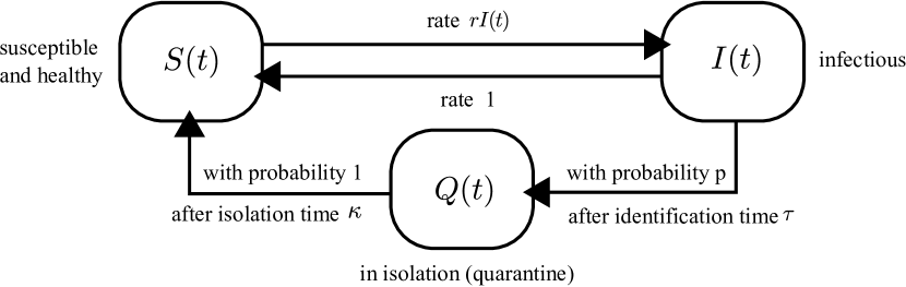
Figure 2.1. Illustration of the SIQ model. The resulting SIQ model is an extension of the SIS model with the additional feature that with probability $p$ individuals that have been infectious for a time $\tau$ are identified and isolated for $\kappa$ units of time at the end of which they are healthy again.

This model neglects several aspects of epidemic scenarios, such as the acquisition of immunity or delays in the development of infectiousness. To demonstrate that the model described above is generalizable, we will, in Sec. 8, introduce an latency period $\sigma$ to become infectious after being infected to the model above, and show how much of the analysis carries over. For conceptual clarity, we will first treat the $\sigma=0$ case in Secs. 3–7.

3. Non-technical overview of the main results

In this section, we describe the main results leaving precise technical formulations for later sections. Recall that without the isolation strategy our SIQ model reduces to the SIS model with disease reproduction number $r$, so that an infection spreads if and only if $r>1$. Of interest in this paper is the case $r>1$, so that if no measures are taken the infection will spread. Consider a history $(\phi_{S}(t),\phi_{I}(t),\phi_{Q}(t)),t\leq 0$, corresponding to the sudden appearance of a small infection at time $t=0$. For definiteness, let $\phi_{Q}(t)=0$ for all $t\leq 0$, $\phi_{I}(t)=0$ for all $t<0$, $0<\phi_{I}(0)\ll 1$, and $\phi_{S}+\phi_{I}+\phi_{Q}\equiv 1$. Unless otherwise stated, this history will be assumed in the discussion below. Our main results can be summarized as follows:

• Required minimum identification probability. We prove that an outbreak can be prevented only if

  (3.1) $$p>p_{c}=1-1/r\ ,$$

  that is, to have a chance to stop the outbreak, one must be able to identify a sufficiently large fraction of infectious individuals.

• Critical identification time. Possessing the ability to detect individuals with probability $p>p_{c}$ alone is not enough; one must be prepared to act with sufficient speed: we prove that for each $p>p_{c}$, there is a critical identification time

  (3.2) $$\tau_{c}(p)=\ln\frac{p}{p_{c}}.$$

  Specifically, for $p>p_{c}$ and $\tau<\tau_{c}$, the infection dies out. In this case, the time $\kappa$ that infectious individuals spend in isolation is of no consequence. These results are presented in Sec. 5.

We can readily compute the critical identification time $\tau_{c}$ for various diseases once we have the reproductive number $r$ and identification probability $p$. In Eqs. (2.1)-(2.1), we have done the usual rescaling $t\mapsto t/\gamma$ where $\gamma$ is the rate of recovery (see the Appendix for a full discussion). This means that $\tau_{c}$ is also rescaled. While that is convenient mathematically, it is also interesting to compare critical identification times without rescaling, so that we can analyze diseases in their natural time spans. To that end, we define

(3.3) $$T_{c}=\frac{\tau_{c}}{\gamma},$$

and show, in Table 2, the critical response capability $p_{c}$ and critical identification time $T_{c}$ for $p=0.8$.

	$r$	$1/\gamma$	$p_{c}$	$T_{c}$
H1N1 2016 [Brazil] [15, 16]	1.7	7.0	0.41	4.7
Ebola 2014 [Guin./Lib.] [17]	1.5	12.0	0.33	10.5
Ebola 2014 [Sierra Leone] [17]	2.5	12.0	0.6	3.5
Spanish Flu 1917 [16]	2	7.0	0.5	3.3
Influenza A [16]	1.54	3.0	0.35	1.0
Hepatitis A [8]	2.25	13.4	0.56	4.89
SARS [8]	2.90	11.8	0.66	4.31
Pertussis [8]	4.75	68.5	0.79	0.91
Smallpox [8]	4.75	17.0	0.79	0.26

Table 2. Critical response capability $p_{c}$ and critical identification time $T_{c}$ (in days) for various diseases with basic reproductive number $r$ as well as $1/\gamma$ (in days). The critical $\tau_{c}$ (before rescaling) is calculated using (3.1)–(3.3) assuming that $80\%$ of infectious individuals are identified and isolated. The values of $r$ and $1/\gamma$ are taken from the references given in the first row.

As shown in Table 2, even when the fraction of identified individuals is as high as $80\%$ the critical identification time $T_{c}$ can be as short as $3$ days for severe outbreaks such as the Spanish Flu and the Ebola in Sierra Leone. Of major concern is what happens if such an identification time is not met. Our next result addresses this scenario.

• Prediction of endemic state as function of $\varepsilon$ and $\kappa$. From Items 1 and 2, we know that when $p<p_{c}$ or $\tau>\tau_{c}$, so that $\varepsilon=pe^{-\tau}<1-\frac{1}{r}$, the infection will persist. When that happens, we prove that if the system tends to an endemic equilibrium, the fraction of infectious individuals in the endemic state will be

  $$I=\frac{1}{1-\varepsilon+\varepsilon\kappa}\cdot\left(1-\varepsilon-\frac{1}{r}\right).$$

  Notice that increasing $\kappa$ leads to an endemic equilibrium with a smaller $I$.

As an illustration consider a hypothetical response to the Ebola outbreak in Sierra Leone with $\varepsilon=0.5$. We obtain that the final fraction of infectious individuals in the endemic state is $I=0.2/({1+\kappa})$.

• Bifurcation analysis at endemic equlibria. For each $p$ and $\tau$ with $\tau\ll 1$, we performed a rigorous bifurcation analysis at each endemic equilibrium point with $\kappa$ as bifurcation parameter. We proved that the equilibrium destabilizes through a Hopf bifurcation as $\kappa$ is increased, and that it undergoes a cascade of Hopf bifurcations as $\kappa$ is increased further.

  
  

• Effect of $\kappa$ on the course of an epidemic. Item 4 described the dynamics near an endemic equilibrium irrespective of how we got there. Here we return to the setting of Item 3, i.e. the sudden appearance of a small infection that gets out of control, and ask how the duration of isolation will influence the course of events. Our results for this part are numerical. We show that the infection will approach the endemic equilibrium predicted in Item 3, and that as $\kappa$ increases, the equilibrium destabilizes through a Hopf bifurcation in a manner similar to that described in Item 4. For large $\kappa$, our simulations suggest that the fraction of infectious individuals, can have periodic oscillations with nontrivial amplitudes. These results are presented in Sec. 7.

To summarize, the SIQ model offers quantitative measures for critical response capabilities and identification times needed to prevent outbreaks of infectious diseases. For endemic infections, our analysis offers guidance to optimal choices of isolation durations. The implications of these results on epidemics control are clear: Isolation of infectious hosts is not without cost, both in terms of society and economics. These must be weighed against the costs of an endemic infection, as well as strategies for disease management. The SIQ model proposed here may assist in such costs-and-benefits analysis.

4. Basic Properties of the Model

4.1. Mathematical framework

Equations (2.1)–(2.3) define a dynamical system on the phase space $C:=C\left(\left[-\tau-\kappa,0\right],\mathbb{R}^{3}\right)$, the Banach space of continuous functions with the norm

$$\left\|\phi\right\|=\sup_{\theta\in\left[-\tau-\kappa,0\right]}\left|\phi\left(\theta\right)\right|\ ,$$

$|\cdot|$ being the Euclidean norm in $\mathbb{R}^{3}$. Given an initial function $\phi\in C$, the solution $x(t,\phi),$ $t\geq 0$, of the initial value problem to (2.1)–(2.3) exists and is unique [18]. We use the standard notation

$$x_{t}(\phi)=x(t+\theta;\phi),\quad\theta\in[-\tau-\kappa,0].$$

This solution defines a $C^{1}$ semiflow $T^{t}:\phi\mapsto x_{t}(\phi)$ on $C$ [18].

Observe that the conservation of mass property of Eqs. (2.1)–(2.3), namely $S^{\prime}(t)+I^{\prime}(t)+Q^{\prime}(t)\equiv 0$, implies that if $\phi=(\phi_{S},\phi_{I},\phi_{Q})$ and $x(t;\phi)=(S(t),I(t),Q(t))$, then $S(t)+I(t)+Q(t)=\phi_{S}(0)+\phi_{I}(0)+\phi_{Q}(0)$ for all $t\geq 0$. In particular, the manifold

$$\mathcal{C}:=\{\phi\in C([-\tau-\kappa,0],\mathbb{R}^{3})\ |\ \phi_{S}(\theta)+\phi_{I}(\theta)+\phi_{Q}(\theta)=1\mbox{ for all }\theta\in[-\tau-\kappa,0]\}$$

is positively invariant with respect to the semiflow $T^{t}$.

In the context of our epidemiological model, all solutions of interest have the property that for each $t$, $x(t;\phi)$ takes value in the $2$-simplex

$$\Delta^{2}=\left\{u=(u_{1},u_{2},u_{3})\in\mathbb{R}^{3}:\sum_{i}u_{i}=1,u_{i}\geq 0,i=1,2,3\right\},$$

i.e., $x_{t}(\phi)\in\tilde{\mathcal{C}}=\{\psi\in\mathcal{C}:\psi(\theta)\in\Delta^{2}\mbox{ for all }\theta\in\left[-\tau-\kappa,0\right]\}$ for all $t\geq 0$. In Sec. 4.3 we show that biologically relevant initial conditions that belong to a certain subset of $\tilde{\mathcal{C}}$ lead to solutions that belong to $\tilde{\mathcal{C}}$ for all $t\geq 0$. When studying $T^{t}$ as a dynamical system, it is conceptually simpler to work with $\mathcal{C}$ as the phase space. We will therefore do that in our theoretical investigations, and focus on trajectories with $T^{t}(\phi)\in\tilde{\mathcal{C}}$ in biological interpretations. Observe that the dynamics on $\mathcal{C}$ are completely determined by any two of Eqs. (2.1)–(2.3) together with the conservation of mass.

4.2. Equilibrium solutions and $\omega$-limit sets

Recall that the $\omega$-limit set $\omega(\phi)$ of $\phi\in\mathcal{C}$ under the semi-flow $T^{t}$ is defined to be

$$\omega(\phi)\ =\ \{\psi\in\mathcal{C}\ |\ T^{t_{n}}\phi\to\psi\mbox{ for some sequence }t_{n}\to\infty\}.$$

For a solution that is bounded, $x_{t}(\phi)$ is $C^{1}$ with a uniform bound on its derivatives for all $t\geq\tau+\kappa$. Thus, by the Arzela-Ascoli Theorem, $\omega(\phi)$ is nonempty and compact in $\mathcal{C}$ (with its $C^{0}$ norm).

In particular, consider an equilibrium solution $\phi$ of Eqs. (2.1)–(2.3), which means that $x\left(t;\phi\right)=\phi\left(0\right)$ for all $t$, and $\phi$ is a constant function. For $u=(u_{1},u_{2},u_{3})\in\mathbb{R}^{3}$ with $\sum_{i}u_{i}=1$, we will use the notation $\hat{u}$ to denote the constant function in $\mathcal{C}$ with $\hat{u}(\theta)=u$ for all $\theta$. The equilibria of Eqs. (2.1)–(2.3) can be computed as follows. If $\hat{\phi}=(\hat{\phi}_{S},\hat{\phi}_{I},\hat{\phi}_{Q})$ is an equilibrium, then it must satisfy

(4.1) $$0=\left(r\left(1-\varepsilon\right)\phi_{S}-1\right)\phi_{I}.$$

Thus any $\hat{\phi}$ with $\phi_{I}=0$ or $\phi_{S}=1/r(1-\varepsilon)$ is an equilibrium solution. We define

$$\mathcal{\mathcal{E}}_{0}:=\left\{\hat{\phi}\in\mathcal{C}|\,\phi_{I}=0\right\}\qquad\mbox{and}\qquad\tilde{\mathcal{E}}_{0}:=\mathcal{\mathcal{E}}_{0}\bigcap\tilde{\mathcal{C}}$$

to be the sets of disease-free equilibria. Analogously we define the sets

$$\mathcal{E}_{I}:=\left\{\hat{\phi}\in\mathcal{C}|\,\phi_{S}=\frac{1}{r\left(1-\varepsilon\right)}\right\}\qquad\mbox{and}\qquad\tilde{\mathcal{E}}_{I}:=\mathcal{E}_{I}\bigcap\tilde{\mathcal{C}},$$

which we refer to as endemic equilibria in the case $\phi_{I}\neq 0$. For $\phi\in\mathcal{C}$, it is possible that $T^{t}(\phi)$ will approach one of the equilibria above as $t\to\infty$, but this need not be the only possible long-time behavior (and we will show that it is not).

4.3. Biologically relevant solutions and their positivity

We consider a solution $x(t;\phi)$ as biologically relevant if $x_{t}(\phi)\in\tilde{\mathcal{C}}$ for all $t\geq 0$. In this section we give sufficient conditions for positivity. More specifically, we show that any initial condition corresponding to an infection that started just prior to $t=0$ leads to a biologically relevant solution.

We start with a function $\psi:\left[-\tau-\kappa,0\right]\to\mathbb{R}^{3}$ (that may or may not be in $\mathcal{C}$). Think of it as a situation we find ourselves in – without knowledge of how we got there. From this initial condition, we evolve the system according to Eqs. (2.1)–(2.3). The next lemma gives conditions on $\psi$ that will lead to biological solutions.

Lemma 1.

Let $\psi=(\psi_{S},\psi_{I},\psi_{Q}):[-\tau-\kappa,0]\to\mathbb{R}^{3}$ be a piecewise continuous function with values in $\Delta^{2}$. We assume further that

$$\psi_{I}(0)\geq rp\int_{-\tau}^{0}e^{\theta}\psi_{S}(\theta)\psi_{I}(\theta)d\theta,$$

and

$$\psi_{Q}(0)\geq r\varepsilon\int_{-\tau-\kappa}^{0}\psi_{S}(\theta)\psi_{I}(\theta)d\theta.$$

Then $S\left(t\right),I\left(t\right),Q\left(t\right)\geq 0$, $S\left(t\right)+I\left(t\right)+Q\left(t\right)=1$ for all $t\geq 0$, and $x_{t}(\psi)\in\tilde{\mathcal{C}}$ for all $t\geq\tau+\kappa$. In particular, if $\psi\in\tilde{\mathcal{C}}$, then $x_{t}(\psi)\in\tilde{\mathcal{C}}$ for all $t\geq 0.$

The proof of Lemma 1 follows from the derivation in the Appendix. Note that the conditions of Lemma 1 are satisfied for open sets of initial conditions corresponding to the sudden uptick of an infection around time $0$, described by $\psi$ with $\psi_{I}(0),\psi_{Q}(0)>0$ and $0<\psi_{I}(t),\psi_{Q}(t)\ll\psi_{I}(0),\psi_{Q}(0)$ for all $t<-\delta$ for some $\delta>0$ sufficiently small.

5. Neighborhood of Disease-Free Equilibria

In Secs. 5.1 and 5.2, we fix $r,$ $p$, $\tau$, and give a complete description of the dynamics in a neighborhood of $\mathcal{E}_{0}$, the set of disease-free equilibria identified in Sec. 4.2. The truly pertinent question, however, is what $\tau$ and $p$ need to be to curb the propagation of small initial infections for a disease the intrinsic reproductive number of which is $r$. These questions will be answered in Sec. 5.3, using the results from the first two subsections.

5.1. Linear analysis at $\mathcal{E}_{0}$

We parametrize $\mathcal{E}_{0}$ by $\widehat{u(q)},$ $q\in\mathbb{R},$ where $u(q)=\left(1-q,0,q\right)$, and study the linearized equation at each point. The following Lemma gives the characteristic equation for a general equilibrium.

Lemma 2.

Let $\hat{w}\in\mathcal{C}$ with $w=\left(w_{S},w_{I},1-w_{S}-w_{I}\right)$ be an equilibrium solution of Eqs. (2.1)–(2.3). Then the characteristic equation at $\hat{w}$ is given by

(5.1) $$\chi\left(\lambda,\hat{w}\right)=0,$$

where

$$\chi\left(\lambda,\hat{w}\right)= \lambda\left(\lambda+1-rw_{S}\left(1-\varepsilon e^{-\tau\lambda}\right)+rw_{I}\left(1-\varepsilon e^{-(\tau+\kappa)\lambda}\right)\right)$$

$$+rw_{I}\varepsilon e^{-\tau\lambda}\left(1-e^{-\lambda\kappa}\right).$$

Since $\mathcal{E}_{0}$ consists of a line of equilibria, $0$ is clearly an eigenvalue for $w_{I}=0$ corresponding to the direction along the line. The stability of these equilibria in directions transverse to $\mathcal{E}_{0}$ is determined by the remaining eigenvalues.

Theorem 3.

Let $\tau$ and $p$ be fixed, and assume $\varepsilon=pe^{-\tau}<1$. We denote

$$q_{c}:=1-\frac{1}{r}\frac{1}{1-\varepsilon}.$$

If $q\geq q_{c}$, then $\widehat{u(q)}$ is linearly stable, and if $q<q_{c}$, then $\widehat{u(q)}$ is linearly unstable. In more detail, at $q\neq q_{c}$, the eigenvalue $\lambda=0$ of the equilibrium $\widehat{u(q)}$ has multiplicity $1$, and there is no other eigenvalue on the imaginary axis. For $q\geq q_{c}$, all nonzero eigenvalues $\lambda$ have $Re(\lambda)<0$. For $q<q_{c}$, there is exactly one eigenvalue $\lambda_{1}$ with $Re(\lambda_{1})>0$.

Proof.

Let $\widehat{u(q)}\in\mathcal{E}_{0}.$ Using Lemma 2, the characteristic equation has the form

(5.2) $$\lambda\left(\lambda+1-r(1-q)\left(1-\varepsilon e^{-\tau\lambda}\right)\right)=0.$$

The eigenvalue $\lambda=0$ of the first factor corresponds to the tangential direction along the manifold $\mathcal{E}_{0}$ and the corresponding normal eigenvalues are remaining solutions of Eq. (5.2). The second factor has a solution $\lambda=0$, if and only if $q=q_{c}$ and it is easy to show that this root is simple. Next we show that $q=q_{c}$ is the only value for which an equilibrium can have a normal eigenvalue $\lambda$ with $Re(\lambda)=0$. The algebraic bifurcation condition $\lambda=i\omega$ implies

(5.3) $$\omega^{2}=\left(r\varepsilon(1-q)\right)^{2}-(1-r(1-q))^{2},$$

(5.4) $$\frac{\omega}{1-r(1-q)}=\tan\left(\omega\tau\right).$$

Equation (5.3) admits solutions $\omega^{2}>0$ if $q\in\left(q_{c},q_{+}\right)$, where $q_{+}=1-\frac{1}{r}\frac{1}{1+\varepsilon}$. Note that the right hand side of Eq. (5.3) attains its global maximum for

$$q_{\max}=1-\frac{1}{r}\frac{1}{1-\varepsilon^{2}}$$

with the corresponding

$$\omega_{\max}^{2}=\frac{\varepsilon^{2}}{1-\varepsilon^{2}}.$$

which satisfies $\left|\omega_{\max}\right|<\frac{\pi}{\tau}$ and thus, we restrict to $\omega\in\left(-\frac{\pi}{\tau},\frac{\pi}{\tau}\right)$. It follows from (5.4) that $\omega=0$ is the only possible solution if and only if

(5.5) $$\frac{1}{1-r(1-q)}\leq\tau,$$

since, in this case, the function $\tan\left(\omega\tau\right)-\omega/\left(1-r(1-q)\right)$ is strictly monotone. In fact, straightforward computation shows that Eq. (5.5) is satisfied for all $q\in\left(q_{-},q_{+}\right)$, $\tau\geq 0$ and $q\in\left[0,1\right]$. Thus, Eqs. (5.3) and (5.4) do not admit solutions with $\omega>0$ and consequently, there are no further bifurcations possible. In particular, there are no Hopf-bifurcations.

Next we show that $Re\left(\lambda\right)<0$ for all nontrivial eigenvalues of all $q\geq q_{c}$. We choose $q=1-\frac{1}{r}>q_{c}$, then (5.2) takes the form $\lambda+\varepsilon e^{-\tau\lambda}=0$, where $\varepsilon\leq 1$. The latter equation only attains solutions with $Re\left(\lambda\right)<0$, see e.g. [19]. Due to continuity, we have $Re\left(\lambda\right)<0$ for all nontrivial eigenvalues for all $q\in\left(q_{c},1\right]\cap\left[0,1\right]$.

For any $q\in[0,q_{c})\cap\left[0,1\right]$, there is exactly one real positive eigenvalue. Indeed, for $q=q_{c}$, the eigenvalue crosses the imaginary axis transversely at $\lambda=0$ with the corresponding derivative

$$\left.\frac{\partial\left(Re\left(\lambda\right)\right)}{\partial q}\right|_{\lambda=0,q=q_{c}}<0.$$

∎

In the context of the epidemic model, of interest is $\tilde{\mathcal{E}}_{0}\subset\tilde{\mathcal{C}}$. We observe that $\hat{u}(q_{c})$ may or may not lie in $\tilde{\mathcal{E}}_{0}$. In particular, if $q_{c}\leq 0$, then all equilibria in $\tilde{\mathcal{E}}_{0}$ are linearly stable.

Corollary 4.

The hypothesis are as in Theorem 3. Then the disease-free equilibrium $\widehat{u}(q)$ is linearly stable if $\tau$ satisfies the inequality

(5.6) $$\tau\leq\tau_{c}(p,q):=\ln p-\ln\left(1-\frac{1}{r(1-q)}\right).$$

Otherwise, it is linearly unstable.

5.2. The nonlinear picture near $\mathcal{E}_{0}$

As the semi-flow $T^{t}$ is $C^{1}$ (Sec. 4.2), we may appeal to invariant manifolds theory. The next theorem follows immediately from results in [20].

Theorem 5.

The hypotheses are as in Theorem 3. Then the following holds:

1. Through every $\widehat{u(q)}$ with $q>q_{c}$ passes a codimension $1$ stable manifold $W^{s}(\widehat{u(q)})$, with uniform estimates away from $\widehat{u}(q_{c})$. These manifolds foliate a uniform size neighborhood of any compact $K\subset\{\widehat{u(q)},q>q_{c}\}$.

2. Through every $\widehat{u(q)}$ with $q<q_{c}$ passes a codimension $2$ stable manifold $W^{s}(\widehat{u(q)})$ and a $1$-dimensional unstable manifold $W^{u}(\widehat{u(q)})$, with uniform estimates away from $\widehat{u(q_{c})}$.

We remark that the $W^{s}$- and $W^{u}$-manifolds above are strong stable and unstable manifolds, i.e., there exist $c=c(q)$ and $\lambda=\lambda(q)>0$ such that

$$\zeta\in W^{s}(\hat{u}(q))\implies\|T^{t}(\zeta)-\hat{u}(q)\|<ce^{-\lambda t}$$

for all $t\geq 0$. The dynamical picture can therefore be summarized as follows: We partition $\mathcal{E}_{0}$ into

$$\mathcal{E}_{0}=\mathcal{E}_{0}^{u}\cup\mathcal{E}_{0}^{c}\cup\mathcal{E}_{0}^{s},$$

where

$$\mathcal{E}_{0}^{u}=\{\widehat{u(q)},q<q_{c}\}\ ,\quad\mathcal{E}_{0}^{c}=\{\widehat{u(q_{c})}\}\ ,\quad\mbox{and}\quad\mathcal{E}_{0}^{s}=\{\widehat{u(q)},q>q_{c}\}\ .$$

For $\phi$ sufficiently near $\mathcal{E}_{0}^{s}$, $I(t)\to 0$ exponentially fast, i.e., the infection dies out quickly; while for $\phi$ sufficiently near $\mathcal{E}_{0}^{u}$, unless $\phi$ lies in the codimensional $1$ submanifold $\cup_{q}W^{s}(\widehat{u(q)})$, $I(t)$ will increase, i.e., the infection will spread, beyond a level depending on the distance of $\phi$ to $\mathcal{E}_{0}^{c}$.

5.3. Critical values of $p$ and $\tau$: scalings and biological implications

We can think of $\tau$, the time between infection and isolation, as identification time, and $p$, the probability of an infectious host to be properly identified and put into isolation, as isolation probability. With these interpretations, a question of practical importance is the following: When presented with a scenario in which a small fraction of the population is infectious, i.e., given an initial condition near $\tilde{\mathcal{E}}_{0}$, what values must $p$ and $\tau$ take to prevent an outbreak, or better yet, to wipe out the infection altogether?

Consider first an initial condition near the equilibirum $(S,I,Q)=(\hat{1},\hat{0},\hat{0})$ as in Sec. 3. In a model with no isolation, the disease reproductive number is known to be $\mathcal{R}_{0}:=r$. Theorem 3 shows that our isolation procedure reduces $\mathcal{R}_{0}$ to the effective disease reproductive number $\mathcal{R}_{\varepsilon}:=(1-\varepsilon)r$; this is a direct rephrasing of the statement that the equilibrium at $(\hat{1},\hat{0},\hat{0})$ is stable if $q_{c}=1-\frac{1}{r}\frac{1}{1-\varepsilon}<0$. Thus starting from near $(\hat{1},\hat{0},\hat{0})$, to beat the infection we have to have $(1-\varepsilon)r<1$, equivalently $\varepsilon>1-\frac{1}{r}$.

We now decipher what this means for $p$ and $\tau$. As $\varepsilon=pe^{-\tau}$, $\varepsilon>1-\frac{1}{r}$ imposes immediately a lower bound on the isolation probability $p$, namely we must have

(5.7) $$p>p_{c}:=1-\frac{1}{r}.$$

Having the capability to identify and properly isolate infectious hosts alone, however, is insufficient. Response time is of the essence: for each $p>p_{c}$, there is a critical identification time

(5.8) $$\tau_{c}(p)=\ln\frac{p}{p_{c}}$$

such that if $\tau>\tau_{c}$, the infection spreads for most initial conditions, whereas $\tau<\tau_{c}$ guarantees that the infection will abate. If $p=p_{c}$, then clearly $\tau_{c}=0$; this implies that isolation has to be immediate upon infection. The farther $p$ is from $p_{c}$, the larger $\tau_{c}(p)$, so that there is a trade-off between probability of isolation and the delay in its implementation.

Consider next an initial condition near the equilibrium $(\widehat{1-q},\hat{0},\hat{q})$ for some fixed $q>0$. Theorem 3 together with an argument analogous to that above shows that in this case, the effective disease reproductive number is $\mathcal{R}_{\varepsilon,q}:=(1-q)(1-\varepsilon)r$. Then $\mathcal{R}_{\varepsilon,q}<1$ is equivalent to $\varepsilon>1-\frac{1}{r(1-q)}$. From this, we deduce the corresponding critical isolation probability $p_{c}(q)$ and critical identification time $\tau_{c}(p,q)$ for each $p$ as before, as in Corollary 4.

An alternate way to understand the effective disease reproductive number $\mathcal{R}_{\varepsilon,q}$ for $q>0$ is as follows: For initial conditions near $(\widehat{1-q},\hat{0},\hat{q})$, a fraction $q$ of the population will never leave isolation, and therefore will not participate in the dynamics. Removing this part of the population from the system changes nothing other than that we will have $S+I+Q=1-q$. Now such a system can be rescaled to one with $\check{S}+\check{I}+\check{Q}=1$, by setting $\check{S}=S/(1-q),\check{I}=I/(1-q)$ and $\check{Q}=Q/(1-q)$, but observe from Eqs. (2.1)–(2.3) that in this rescaling $r$ is changed as well; it becomes $\check{r}=(1-q)r$, consistent with the relation between $\mathcal{R}_{\varepsilon}$ and $\mathcal{R}_{\varepsilon,q}$ above.

Finally, we remark that the value of $q_{c}$, which fully dictates the stability properties of the disease-free equilibria, depends only on $p$ and $\tau$ and not on $\kappa$. That is to say, response capabilities matter, but isolation duration does not, with regard to the prevention of outbreaks.

6. Away from Disease-free Equilibria

We now move away from $\mathcal{E}_{0}$, the set of disease-free equilibria, to explore dynamics on a more global scale. The condition $p>0$ is assumed throughout.

6.1. An integral of motion

It has been pointed out that by construction epidemiological models including delayed terms oftentimes satisfy some secondary invariant integral condition [21]. It turns out that in addition to mass conservation, Eqs. (2.1)–(2.3) possess a second conserved quantity. Let $r$ and $\kappa$ be fixed. We define $H=H^{r,\kappa}:\mathcal{C}\to\mathbb{R}$ by

(6.1) $$H\left(\phi\right):=1-\phi_{S}(0)-\phi_{I}(-\kappa)+\negmedspace\int\limits_{-\kappa}^{0}(1-r\phi_{S}(s))\phi_{I}(s)\mbox{d}s$$

where $\phi=(\phi_{S},\phi_{I},\phi_{Q})$.

Proposition 6.

For each fixed $r,\kappa$,

$$\frac{d}{dt}H(x_{t}(\phi))=0\qquad\mbox{for all }\phi\in\mathcal{C}\mbox{ and }t\geq 0,$$

and the level sets of $H$ define a smooth foliation on $\mathcal{C}$.

Proof.

Writing $x(t;\phi)=(S(t),I(t),Q(t))$ for $t\geq 0$, we have

$$\frac{d}{dt}H(x_{t}(\phi))=-\dot{S}(t)-\dot{I}(t-\kappa)+(1-rS(t)I(t)-(1-rS(t-\kappa))I(t-\kappa),$$

which one checks is equal to $0$ by plugging into Eqs. (2.1)–(2.3). To show that the level sets of $H$ are codimension 1 submanifolds, it suffices to check, by the Implicit Function Theorem, that $D_{\phi}H$, the derivative of $H$, is surjective at each $\phi$. This is true, as for any $\phi$ there exits a $\psi=(\psi_{S},\psi_{I},\psi_{Q})$ such that

$$(D_{\phi}H)\psi=-\psi_{S}(0)-\psi_{I}(-\kappa)+r\negmedspace\int\limits_{-\kappa}^{0}(1-r\phi_{S}(s))\psi_{I}(s)\mbox{d}s-r\negmedspace\int\limits_{-\kappa}^{0}\phi_{I}(s)\psi_{S}(s)\mbox{d}s\neq 0,$$

For example, choose $\psi_{I}=\hat{0}$, $\psi_{S}(\theta)=0$ for all $\theta\in[-\tau-\kappa,-\delta]$ and $\psi_{S}(\theta)=1-\theta/\delta$ for $\theta\in[-\delta,0]$, where $0<r\delta<1/\sup\phi_{I}$. ∎

For fixed $r$ and $\kappa$, we let $\mathcal{F}=\mathcal{F}^{r,\kappa}$ denote the foliation given by Proposition 11, and let $\mathcal{F}_{q}:=H^{-1}(q)$. Then $\mathcal{F}_{q}$ is invariant under the semi-flow, i.e., for $\phi\in\mathcal{F}_{q}$, $x_{t}(\phi)\in\mathcal{F}_{q}$ for all $t\geq 0$. We consider below the intersection of $\mathcal{F}_{q}$ with the set of equilibrium points for arbitrary $\kappa$ and $q$.

Theorem 7.

For fixed $r,\kappa,q$, we let $\mathcal{F}=\mathcal{F}^{r,\kappa}$, and consider $\mathcal{F}_{q}$.

1. Then $\mathcal{F}_{q}\cap\mathcal{E}_{0}=\{\widehat{u(q)}\}$, where $u(q)=(1-q,0,q)$.

2. Fixing additionally $p,\tau$, which determines $\mathcal{E}_{I}=\{\phi_{S}=[r(1-\varepsilon)]^{-1}\}$, we have $\mathcal{F}_{q}\cap\mathcal{E}_{I}=\{\widehat{v(q)}\}$, where $v(q)=(v_{S},v_{I}(q),v_{Q}(q))$ and

   $$v_{I}(q)=\frac{1-\varepsilon}{1-\varepsilon+\varepsilon\kappa}\left(q_{c}-q\right),$$

   (6.2) $$v_{Q}(q)=\frac{\varepsilon\kappa}{1-\varepsilon+\varepsilon\kappa}\left(q_{c}-q\right).$$

These assertions follow from straightforward computations.

We remark on how the leaves of $\mathcal{F}^{r,\kappa}$ vary with $\kappa$. Setting $\kappa=0$, we see from (6.1) that $\mathcal{F}_{q}=\{\phi_{Q}(0)=q\}$. For small $\kappa>0$, it is easy to see that the leaves $\mathcal{F}_{q}^{r,\kappa}$ are “close” to those of $\mathcal{F}_{q}^{r,0}$. Observe from the formulas above that with $p$ and $\tau$ fixed, $v_{I}(q)$ decreases monotonically as $\kappa$ increases. Indeed the leaf $\mathcal{F}^{r,\kappa}_{q}$ “bends” away from $\mathcal{F}^{r,0}_{q}$ increasingly, its intersection with $\mathcal{E}_{I}$ tending to $(\widehat{1-q_{c}},\hat{0},\hat{q}_{c})$ as $\kappa\to\infty$.

6.2. Discussion

Fixing $r,\kappa$ and starting from $\phi$ with $\phi_{I}\ll 1$, one asks what the future holds. For fixed $p,\tau$, suppose $\phi\in\mathcal{F}_{q}$ for some $q$. If $q>q_{c}$, then $x_{t}(\phi)\to\widehat{u(q)}\in\mathcal{F}_{q}\cap\mathcal{E}_{0}$ as $t\to\infty$ by Theorem 3, if $\phi$ was chosen in some sufficiently small neighborhood of $\mathcal{E}_{0}$. We focus therefore on the case $q<q_{c}$, for which we have to expect $x(t;\phi)$ to move away from the set of disease-free equilibria $\mathcal{E}_{0}$.

One possibility is for $x_{t}(\phi)$ to tend to $\widehat{v(q)}$, the unique point in $\mathcal{F}_{q}\cap\mathcal{E}_{I}$, as $t\to\infty$. It is difficult to determine if, or under what conditions, this occurs; such nonlocal dynamical behaviors are very challenging to analyze. We have some evidence that this is not an unreasonable expectation, at least for smaller values of $\kappa$, and confirmed this with numerical simulations; see Figure 6.1.

Not all endemic equilibria identified in Sec. 4.2 are reachable if one starts from an initial condition $\phi$ near $\tilde{\mathcal{E}}_{0}$. For each $r,p,\tau,\kappa$, we define the set of reachable endemic equilibria $\mathcal{E}_{I}^{r,p,\tau,\kappa}$ to be those equilibrium points in $\mathcal{E}_{I}$ that are, in principle, reachable starting from a biologically realistic initial condition, i.e.,

$$\mathcal{E}_{I}^{r,p,\tau,\kappa} = \{\hat{v},v=(v_{S},v_{I}(q),v_{Q}(q)),q\in[0,1],q<q_{c}\}\ ,$$

where $v_{S},v_{I}(q)$ and $,v_{Q}(q)$ are as in Theorem 7.

In the scenario that $x_{t}(\phi)$ tends to $\hat{v}$, Theorem 7 tells us it is advantageous to use a larger $\kappa$, for the longer one keeps infectious hosts in isolation, the smaller the $I$-component $v_{I}$ of the asymptotic state $\hat{v}$. If $\hat{v}$ is unstable, then convergence to it is unlikely, and the structures that emerge from $\hat{v}$ after it loses stability become candidates for the $\omega$-limit set of $\phi$, which we know is nonempty if $x(t;\phi)$ is bounded (by the remark at the end of Sec. 4.2). This motivates the eigenvalue analysis of the equilibria in $\mathcal{E}_{I}$ in the next section.

Figure 6.1. Convergence to $\mathcal{\tilde{E}}_{I}$ for initial conditions close to $\tilde{\mathcal{E}}_{0}$. Here $p=\frac{1}{2},\tau=0.5$. Initial conditions are of the form $\phi(\theta)=(1,0,0)$ for all $\theta<0$ and $\phi(0)=(0.999-q,0.001,q)$ for 10 equidistant values of $0\leq q\leq q_{c}$. Panel (a): $\kappa=0.5$. Panel (b): $\kappa=5$. Curves show trajectories in direction of arrows projected onto $(Q,I)$-space.

7. The case of an endemic infection

In Secs. 7.1 and 7.2, we study the dynamics close to $\mathcal{E}_{I}$, the set of endemic equilibria defined in Sec. 4.2. For fixed $r>1,p\in(0,1)$ and $\tau=0$, we give in Sec. 7.1 a complete bifurcation analysis of each equilibrium point in $\mathcal{E}_{I}$ as $\kappa$ increases. These results remain valid for small $\tau>0$. In Sec. 7.2, we deduce from the linear analysis above nonlinear behaviors in neighborhoods of these equilibria.

While Secs. 7.1 and 7.2 are concerned with the dynamical picture near an endemic equilibrium irrespective of how one gets there, Sec. 7.3 addresses the following very pertinent question: Given an initial condition $\phi$ with small $\phi_{I}>0$, if one is unable to control the outbreak, which $\kappa$, i.e., what durations of isolation, will best mitigate the severity of the infection? As we will show, the dynamical landscape is quite complex. Results of numerical computations will be presented to clarify the situation.

7.1. Linear analysis at $\mathcal{E}_{I}$

Let $r$ and $\varepsilon$ be fixed throughout. We parametrize $\mathcal{E}_{I}$ by $\widehat{w(q)},\,q\in\mathbb{R},$ where $w\!\left(q\right)=\left(1-q_{c},q_{c}-q,q\right)$ and study the linearized equation at each point. Clearly, $0$ is an eigenvalue, as $\mathcal{E}_{I}$ is a line of equilibria. We have the following result for $\kappa=0$.

Proposition 8.

Let $\tau$ and $p\in(0,1)$ be fixed, and $\kappa=0$. If $q\leq q_{c}$ then $\widehat{w(q)}$ is linearly stable; otherwise it is linearly unstable.

Specifically, for $q<q_{c}$, the eigenvalue $\lambda=0$ has multiplicity 1 and all other eigenvalues satisfy $Re\left(\lambda\right)<0$, and one eigenvalue crosses the imaginary axis as $q$ increases past $q_{c}$.

The proof of Proposition 8 is analogous to the proof of the stability of disease-free equilibria in Theorem 3. More specifically, for the case $\kappa=0$, the corresponding characteristic equation is

(7.1) $$\lambda\left(\lambda+1-r\left(1-q-2(q_{c}-q)\right)\left(1-\varepsilon e^{-\tau\lambda}\right)\right)=0,$$

which has the same form as Eq. (5.2) from Theorem 3. Therefore, the statement of Proposition 8 can be proven by similar arguments.

We remark that the stability persists at least for small values of $\kappa$ for all points $\widehat{w(q)}$, $q\neq q_{c}$. Moreover, a uniform estimate for such $\kappa$ can be obtained by excluding a neighborhood of the point $\widehat{w(q_{c})}$.

For $q<q_{c}$, even as Proposition 8 tells us that $\widehat{w(q)}$ is stable for small $\kappa$, there is no guarantee that it will not destabilize for larger values of $\kappa$. We first give a rigorous analysis for the case $\tau=0$, fixing $q$ and letting $\kappa$ increase, as there are standard techniques for investigating asymptotic properties of the spectrum as the delay increases. We refer to [22] for a general overview of the concepts used in the proof of the following theorem.

Theorem 9.

Let $0<p<1$ and $\tau=0$ be fixed. Then, there exist $q_{h}^{-},q_{h}^{+}$ for which the following hold: If $q\in\left[q_{h}^{-},q_{h}^{+}\right]$ and $q<q_{c}$, then $\widehat{w(q)}$ is linearly stable for all $\kappa\geq 0$. For $q$ such that $q\notin\left[q_{h}^{-},q_{h}^{+}\right]$ and $q<q_{c}$, we have the following.

1. There exists $\kappa_{0}(q)$ such that $\widehat{w(q)}$ is linearly stable for $\kappa\leq\kappa_{0}(q)$ and linearly unstable for $\kappa>\kappa_{0}(q)$.

2. For $\kappa=\kappa_{0}(q)$, the linearization at $\widehat{w(q)}$ possesses a pair of purely imaginary eigenvalues $\pm i\Omega(q)$, $\Omega(q)>0$, crossing the imaginary axis with positive speed as $\kappa$ increases.

3. For each $\kappa_{m}(q)=\kappa_{0}(q)+m2\pi/\Omega(q)$, $m\in\mathbb{N}$, $\widehat{w(q)}$ possesses a pair of purely imaginary eigenvalues $i\Omega(q)$, crossing the imaginary axis with positive speed.

For $q<q_{c}$, these are the only bifurcations as $\kappa$ is varied.

The results of Theorem 9 carry the following biological interpretation: Suppose we find ourselves near an endemic equilibrium. How we got there is of no concern – be it due to natural calamity, large stochastic fluctuations, viral mutation – what matters is that we are there, and the question is: what are the effects of prolonged periods of isolation? Theorem 9 gives a complete answer to this question on the linear level.

Proof of Theorem 9.

We compute the eigenvalues of the linearization at $\widehat{w(q)}$. By Lemma 2, the characteristic equation at $\widehat{w(q)}$ reads

(7.2) $$\chi\left(\lambda,\widehat{w(q)},\kappa\right)= \lambda\left(\lambda+1-r\left(1-q_{c}\right)\left(1-\varepsilon e^{-\tau\lambda}\right)+r\left(q_{c}-q\right)\left(1-\varepsilon e^{-\tau\lambda}Y(\lambda)\right)\right)$$

$$+r\left(q_{c}-q\right)\varepsilon e^{-\tau\lambda}\left(1-Y(\lambda)\right),$$

where we use the notation $e^{-\lambda\kappa}=:Y(\lambda)$. Note that the solution $\lambda_{0}=0$ of (7.2) corresponds to the direction tangential to the line $\mathcal{E}_{I}$. We use the result from [22], which describes the asymptotic properties of the spectrum for large delay (here $\kappa$). More specifically, the spectrum for large $\kappa$ can be described by two parts: the strong spectrum $\lambda$ such that $\lambda=\mathcal{O}\left(1\right)$ as $\kappa\to\infty$, which is given by the solutions of the equation

(7.3) $$\lambda\left(\lambda+1-r\left(1-q_{c}\right)\left(1-\Lambda\left(\lambda\right)\right)+r\left(q_{c}-q\right)\right)+r\left(q_{c}-q\right)=0,$$

(Eq. (7.2) for $Y=0$) with positive real parts, and the so called asymptotic continuous spectrum with $\mbox{Re}\,\lambda=\mathcal{O}\left(1/\kappa\right)$ as $\kappa\to\infty$. For $\tau=0$, Eq. (7.3) has the solutions

$$\lambda_{\pm}=\frac{1}{2}\left[-r\left(1-p\right)\left(q_{c}-q\right)\pm\sqrt{\left(q_{c}-q\right)\left(r^{2}\left(1-p\right)^{2}\left(q_{c}-q\right)-4p\right)}\right],$$

satisfying $Re(\lambda)<0$ for all $q\in\left[0,q_{c}\right)$, which means that the strong spectrum is absent. The asymptotic continuous spectrum is given by $\lambda=-\frac{1}{\kappa}\gamma\left(\omega\right)+i\omega$ where $\gamma\left(\omega\right)=-\frac{1}{2}\log\left|Y(i\omega)\right|^{2}$, and $Y(\cdot)$ can be computed by solving (7.2) with respect to $Y$ (see more details in [22, 23])

$$Y(\lambda) = \frac{\lambda^{2}+\lambda\left(1+r\left(1-q\right)+\frac{1}{1-\varepsilon}\Lambda\left(\lambda\right)\right)+r\left(q_{c}-q\right)\Lambda\left(\lambda\right)}{r\left(q_{c}-q\right)\Lambda\left(\lambda\right)\left(\lambda+1\right)}.$$

It is straightforward to compute that $\gamma\left(0\right)=0.$ Moreover, $\frac{\partial\left|Y\right|}{\partial\omega}(0)=0$ and $\frac{\partial^{2}\left|Y\right|}{\partial\omega^{2}}(0)=h(q)$ with

$$h\left(q\right)=\left(\frac{1-r\left(1-p+\left(p-2\right)q_{c}-q\right)}{pr\left(q_{c}-q\right)}\right)^{2}-\frac{2}{pr\left(q_{c}-q\right)}-1.$$

Hence, $\frac{\partial^{2}Y}{\partial\omega^{2}}(0)$ changes sign when $h(q)=0$. In particular, $h(q)<0$ corresponds to the so-called modulational instability [23]. Simple analysis of the function $h(q)$ shows that $h\left(q\right)\geq 0$ for all $q\in\left[q_{h}^{-},q_{h}^{+}\right]\neq\emptyset,$ where

(7.4) $$\left(1-p^{2}\right)\left(q_{c}-q_{h}^{\pm}\right)=a+p\mp\sqrt{\left(a+p\right)^{2}-\left(1-p^{2}\right)a^{2}}$$

and $a=p_{c}-p+\left(p-3\right)q_{c}$. In this case, $\gamma\left(\omega\right)$ is concave and $\gamma\left(\omega\right)<0$ for all $\omega\in\mathbb{R}\setminus\left\{0\right\}.$ As a result, there are no eigenvalues with positive real part for sufficiently large $\kappa$. In contrast, for all $q\notin\left[q_{h}^{-},q_{h}^{+}\right]$ there exists an open set $I_{\Omega}:=\left(-\Omega,\Omega\right)\setminus\left\{0\right\}$ such that $\gamma(\pm\Omega)=0$ and the pseudo-continuous spectrum $\gamma(\omega)>0$ for $\omega\in I_{\Omega}\setminus\left\{0\right\}$. Hence, as follows from [22] for large $\kappa$ there exists at least one pair of complex conjugated eigenvalues with positive real parts and nonzero imaginary parts. With the increasing of $\kappa$, these eigenvalues have to cross the imaginary axis at $\pm i\Omega$. We denote the corresponding value of $\kappa$, where this occurs as $\kappa_{0}(q)$.

Hence, it holds that $\chi\left(\pm i\Omega(q),\widehat{w(q)},\kappa_{0}(q)\right)=0$ for some $\kappa_{0}(q)>0$. Then, for $\kappa_{m}(q)=\kappa_{0}(q)+m2\pi/\Omega(q)$, $m\in\mathbb{N}$ it holds

$$\chi\left(\pm i\Omega(q),\widehat{w(q)},\kappa_{m}(q)\right)=\chi\left(\pm i\Omega(q),\widehat{w(q)},\kappa_{0}(q)\right)=0,$$

since $\left.Y\left(\pm i\Omega\right)\right|_{\kappa_{m}}=e^{\mp i\Omega\kappa_{m}}=e^{\mp i\Omega\kappa_{0}}=\left.Y\left(\pm i\Omega\right)\right|_{\kappa_{0}}.$ This implies the existence of purely imaginary eigenvalues at all values $\kappa_{m}(q)$, which form the diverging monotone sequence of delay values for each point $\widehat{w(q)}$. ∎

Figure 7.1. Asymptotic spectral properties of a given equlibrium $\widehat{w(q)}\in\tilde{\mathcal{E}}_{I}$ for large values of $\kappa$. All eigenvalues close to the imaginary axis lie on invariant curves with shapes indicated as above. In particular, $\lambda=0$ is an eigenvalue and the distance between two neighboring eigenvalues on these curves is approximately $2\pi/\kappa$. The shapes can be distinguished by the sign of the auxilliary variable $h(q)$ introduced in the proof of Theorem 9, where the case $h(q)<0$ corresponds to the so called modulational instability, see Ref. [22].

By standard theory, eigenvalues at $\widehat{w(q)}$ for small $\tau>0$ are close to those at $\tau=0$. Thus for each $\kappa$ away from bifurcation points, $\widehat{w(q)}$ has the same number of unstable eigenvalues for small $\tau$ as in the theorem above, with the size of the allowed perturbation in $\tau$ depending on $\kappa$. See Fig 7.1 for graphic visualization of the spectral properties described above. We have also computed numerically the regions of stability for a range of values of $q$ and $\kappa$; they are shown in Fig. 7.2.

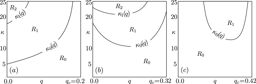
Figure 7.2. Stability of the endemic equilibria $\widehat{w(q)}\in\tilde{\mathcal{E}}_{I}$ as function of $q$ and $\kappa$. Here $r=2.5$, $p=0.5$. Panel (a): $\tau=0$, Panel (b): $\tau=0.2$, Panel (c): $\tau=0.5$. Each panel shows $q\in[0,q_{c}]$ in the $x$-axis, and $\kappa\in[0,25]$ in the $y$-axis. The square is partitioned into $R_{0}=\{(q,\kappa):\kappa<\kappa_{0}(q)\}$, $R_{i}=\{(q,\kappa):\kappa_{i-1}(q)<\kappa<\kappa_{i}(q)\},\ i=1,2$. Drawing a vertical line through the square, one witnesses the implications of Theorem 9; that is, for fixed $0\leq q<q_{c}$, the equilibrium $\widehat{w(q)}$ is increasingly destabilized as $\kappa$ increases. Drawing a horizontal line, one sees at a glance the regions of stability and instability for each $\kappa$.

7.2. The nonlinear picture near $\mathcal{E}_{I}$

As the semi-flow $T^{t}$ is $C^{1}$ (see Sec. 3.1), we have at our disposal stable and unstable manifolds theory to further clarify the nonlinear picture near $\mathcal{E}_{I}$ as was done for $\mathcal{E}_{0}$. Additionally, we know from Sec. 6.1 that for each $r,\kappa,p,\tau$, there is a $T^{t}$-invariant, codimension 1 foliation $\mathcal{F}=\mathcal{F}^{r,\kappa}$ transversal to $\mathcal{E}_{I}$. Below we let $\mathcal{F}_{q^{\prime}}$ be the leaf of $\mathcal{F}$ passing through $\widehat{w(q)}$, so that $q^{\prime}$ and $q$ are related by $q=v_{Q}(q^{\prime})$ where $v_{Q}$ is as in Theorem 7.

Consider $q<q_{c}$. By Proposition 8, for $\kappa<\kappa_{0}$, $\widehat{w(q)}$ is an attractive fixed point for the dynamics on $\mathcal{F}_{q^{\prime}}$, so that any orbit on $\mathcal{F}_{q^{\prime}}$ coming to within a certain distance of $\widehat{w(q)}$ (measured along $\mathcal{F}_{q^{\prime}}$) will converge to it. For $\kappa<\kappa_{0}$ and close enough $\kappa_{0}$, we know from the complex conjugate eigenvalues at $\widehat{w(q)}$ that any such trajectory will exhibit damped oscillatory behavior as it tends to its endemic equilibrium. Though not necessarily the case, this will likely be reflected also in $I(t)$, the fraction of population infectious. Though Theorem 9 cannot be applied directly to the situation depicted in Fig 6.1(b), the presence of complex eigenvalues is consistent with the way some of the trajectories spiral toward their endemic equilibria.

At $\kappa=\kappa_{0}\left(q\right)$, a Hopf bifurcation occurs at $\widehat{w(q)}$. Though technical conditions are difficult to check, in a generic super-critical Hopf bifurcation what happens is that for $\kappa$ just past $\kappa_{0}$ a small limit cycle emerges from $\widehat{w(q)}$. More precisely, restricted to $\mathcal{F}_{q^{\prime}}$, the dynamics near $\widehat{w(q)}$ can be described as follows: There is a strong stable manifold, codimension 2 with respect to $\mathcal{F}_{q^{\prime}}$, and a 2D center manifold passing through $\widehat{w(q)}$. All orbits on $\mathcal{F}_{q^{\prime}}$ that are within a certain distance of $\widehat{w(q)}$ are driven towards the 2D center manifold, towards the small limit cycle bifurcating from $\widehat{w(q)}$. This dynamical picture persists as $\kappa$ increases, at least for a little while; the limit cycle grows larger and becomes more robust.

By the time $\kappa$ reaches $\kappa_{1}$, it is difficult to know if the picture above still persists. If it does, then what happens as $\kappa$ increases past $\kappa_{1}$ is that the codimension 2 strong stable manifold within $\mathcal{F}_{q^{\prime}}$ becomes codimension 4, and orbits on $\mathcal{F}_{q^{\prime}}$ near $\widehat{w(q)}$ are driven towards a 4D center manifold. A second frequency of oscillation with small amplitude develops around the existing larger and more robust limit cycle. At each $\kappa_{m}$, the dimension of the center manifold goes up by 2.

7.3. Optimizing isolation durations

In the last two subsections, we have focused on the dynamical properties near specific equilibria in $\mathcal{E}_{I}$ for specific parameters. That information is useful, but the question of practical importance here is the following. Suppose we find ourselves at some $\phi=(\phi_{S},\phi_{I},\phi_{Q})\in\tilde{\mathcal{C}}$ with $0<\phi_{I}\ll 1$, and the response capabilities, i.e. $p$ and $\tau$, are such that they are not sufficient for preventing an outbreak given the reproductive number $r$ of the disease. That is to say, $\phi_{Q}(0)<q_{c}$. Accepting that the infection will become endemic, the question is: will some lengths of isolation be more effective in mitigating the outbreak, and are there optimal choices of $\kappa$? Assuming $r,p$ and $\tau$ are fixed, we propose the following two sets of considerations:

The potential endemic equilibrium. First, there is the endemic equilibrium to which $x(t;\phi)$ may – or may not – eventually tend. This can be computed as follows: For each $\kappa$, we compute $q^{\prime}:=H^{r,\kappa}(\phi)$ where $H$ is as in Sec. 6.1. This determines $\mathcal{F}_{q^{\prime}}$, the leaf of the foliation $\mathcal{F}^{r,\kappa}$ containing the initial condition $\phi$. From (6.2), we compute explicitly $I(\phi,\kappa)=v_{I}(q^{\prime})$, the $I$-coordinate of the the point in $\mathcal{E}_{I}$ to which the trajectory from $\phi$ may potentially be attracted if the duration of isolation is $\kappa$.

Fig. 7.3(a) shows the trajectories for a few initial conditions with $0<\phi_{I}\ll 1$ close to the point $(\hat{1},\hat{0},\hat{0})$ in $\tilde{\mathcal{E}}_{0}$. Here we see that for $\kappa$ up to about 10, the solution converges to a stable equilibrium, with what appears to be a Hopf bifurcation occurring around $\kappa=10$. This is related to, though not strictly the same as, the Hopf bifurcation in Theorem 9: here as we vary $\kappa$, the point in $\mathcal{E}_{I}$ changes with it. Long before this bifurcation, the complex conjugate eigenvalues of the points in $\mathcal{E}_{I}$ (see Theorem 9) are clearly visible, as the solutions spiral toward the equilibria. This translates into oscillatory behavior for $I(t)$, the fraction of the population that is infectious. Before the bifurcation, these oscillations are damped; the damping grows weaker and eventually disappears altogether. As shown in Fig. 7.3(b), for larger $\kappa$, the solutions tend to limit cycles which appear to grow in size, with $I(t)$ rising periodically higher than some of the stable equilibria to which solutions tend for smaller $\kappa$.

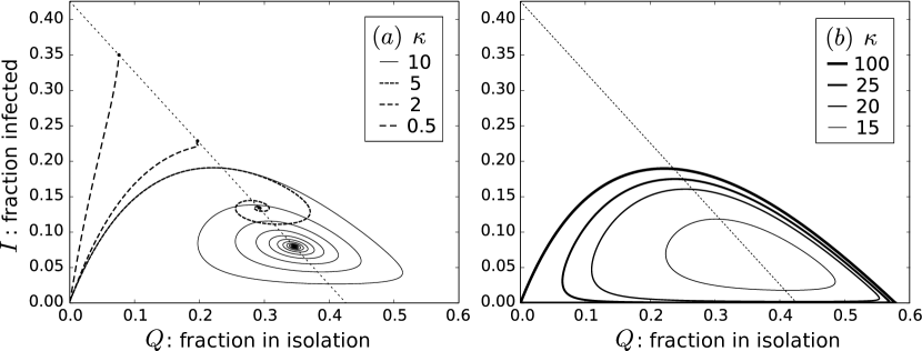
Figure 7.3. Long term behavior for solutions with set initial condition close to $\mathcal{\tilde{E}}_{0}$. Fix $p=\frac{1}{2}$, $\tau=0.5$ and initial condition $\phi$, such that $\phi(\theta)=(1,0,0)$ for all $\theta\in[-\tau-\kappa,0)$ and $\phi(0)=(0.99,0.01,0)$ (Lemma 1 guarantees that $x_{t}(\phi)\in\tilde{\mathcal{C}}$ for all $t\geq\tau+\kappa$). Panel (a): For small values of $\kappa$ the solution $x_{t}(\phi)$ converges to some $\hat{v}\in\mathcal{\tilde{E}}_{I}$ given by Theorem 7. The rate of convergence, however, decreases as $\kappa$ grows until there is a super-critical Hopf-bifurcation and the solution $x(t;\phi)$ converges to a limit cycle. Panel (b): Limit cycles of $x(t;\phi)$ for $\kappa\in\left\{15,20,25,100\right\}.$ See also Fig. 7.2(b).

We remark that the trajectories depicted in Fig 6.3 are likely representatives of trajectories starting near $\phi$. This is because through each $\widehat{u(q)}$ where $u(q)=(1-q,0,q)$ with $q<q_{c}$, there is, within $\mathcal{F}_{q}$, a codimension-1 stable manifold $W^{s}$ and a 1D unstable manifold $W^{u}$. Starting from any $\phi\in\mathcal{F}_{q}$ with $\phi_{I}\ll 1$, assuming $\phi\not\in W^{s}$, its trajectory will follow $W^{u}$, which consists of a single trajectory. As this is true for all $\phi\in\mathcal{F}_{q}$ with $\phi_{I}\ll 1$, examining where one trajectory goes will tell us about all such trajectories.

The maximum outbreak size. Above we were concerned with the large-time dynamics of the disease, the eventual level of infection. Here we look at the transient dynamics before this asymptotic state is reached. For each $\phi$ and $\kappa$, we define

$$I_{{\rm peak}}(\phi,\kappa)=\sup_{t\geq 0}\ I(t)$$

where $I(t)$ is the $I$-component of $x(t;\phi)$. This is a very relevant quantity, as too large an $I_{{\rm peak}}$-value is clearly unacceptable even if eventually the disease winds down.

Fig. 7.4 shows this quantity as a function of $\kappa$ for the same $\phi$ in Fig. 7.3 for a few values of $\tau$. These plots show that $I_{{\rm peak}}$ is a decreasing function which levels off beyond a certain point, i.e., even though $I(\phi,\kappa)$ continues to decrease with increasing $\kappa$, the worst of the epidemic does not improve. That is to say, the time course of the infection is such that it will first get worse, and only after a certain fraction of the population is infectious that it will start to abate, due to the effect of isolation, which diminishes the size of the susceptible population.

Figure 7.4. Values of $I_{{\rm peak}}$ for $r=2.5,p=0.5$ as functions of $\kappa\in[0,25]$ for fixed $\tau\in\left\{0.1,0.5,1\right\}$ and initial condition $\phi(\theta)=(1,0,0)$ for all $\theta<0$ and $\phi(0)=(0.999,0.001,0)$.

Here is a rigorous argument for why $I_{{\rm peak}}$ is bounded below by a positive value independent of $\kappa$: Consider the limiting case $\kappa=\infty$, i.e., individuals that enter the state $(Q)$ remain there forever. The unstable manifold at the point $(\hat{1},\hat{0},\hat{0})$ is a curve whose $I$-component increases initially and must eventually tend to $0$ as the entire population is in $(Q)$. Denoting the maximum value of the $I$-component of this unstable curve by $\tilde{I}_{{\rm peak}}$, it is easy to see that for $\phi$ with $0<\phi_{I}\ll 1$ near $(\hat{1},\hat{0},\hat{0})$ and any $\kappa$, we must have $I_{{\rm peak}}(\phi,\kappa)\geq\tilde{I}_{{\rm peak}}$: the part of the population that leaves isolation becomes susceptible and can only contribute to a larger $I(t)$.

Finally, we discuss the question posed at the beginning of this section: What constitutes an optimal value of $\kappa$, in the setting above where $p$ and $\tau$ are fixed and $\phi$ is given? First one has to decide whether it is the value of $I_{{\rm peak}}$ that matters, or the eventual level of infection. With regard to large-time dynamics, there is also the following consideration: If the trajectory tends to an equilibrium $\hat{w}\in\mathcal{E}_{I}$, then obviously the smaller the $I$-component of $\hat{w}$, the better. As noted in Theroem 7, this means taking as large $\kappa$ as we can. But too large a value of $\kappa$ is also impractical. Also, for larger values of $\kappa$, $\hat{w}$ can destabilize, with the trajectory accumulating on a limit cycle, as shown in Fig. 7.3. This means $I(t)$ will oscillate forever periodically in time, with potentially higher peaks (as well as lower troughs) than for the stable equilibria for smaller $\kappa$. Which scenario is more desirable or can be better tolerated is not a mathematical question; it depends on factors such as the nature of the disease, hardships at peak times, possibilities of intervention when the infection ebbs, and so on. All we can offer is knowledge of which $\kappa$ will lead to what kinds of large-time dynamics for $I(t)$.

8. Extension: latency time

We discuss in this section a simple extension of the SIQ model, one that includes the idea of an latency period. This model divides the population into four groups, “S” for healthy and susceptible, “E” for exposed but not yet infectious, “I” for infectious, and “Q” for isolation. The only change in the dynamics is as follows: Suppose an individual from Group S gets infected at time $t$. He enters Group E immediately and remains there for $\sigma$ units of time, $\sigma\geq 0$ being a constant we will refer to as the latency period. For simplicity we assume that while in Group E, the individual is neither infectious (so he can infect no one), nor symptomatic (so he cannot be identified and isolated), nor does recovery begin. At time $t+\sigma$, he becomes infectious, enters Group I, and from this point on, the rules for identification, isolation, and recovery are the same as before. The parameters in this extended model, which we call SEIQ, are $r,\sigma,p,\tau$ and $\kappa$. A schematic is shown in Fig. 8.1.

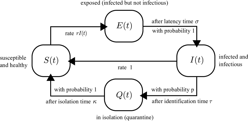
Figure 8.1. Illustration of the SEIQ model. Extension of the SIQ model with the additional feature that once infected (here referred to as $E(t)$ for exposed), individuals undergo an latency period of length $\sigma$ before becoming infectious.

We will follow a line of analysis similar to that in Secs. 3–7. Note how the structures of SIQ persist and extend to the case with latency.

8.1. Mathematical set up and the set of equilibrium points

First we write down the corresponding system of Delay Differential Equations, derived in the same way:

(8.1) $$\dot{S}\negmedspace\left(t\right) = -rS\negmedspace\left(t\right)I\negmedspace\left(t\right)+I\negmedspace\left(t\right)+r\varepsilon S\negmedspace\left(t-\sigma-\tau-\kappa\right)I\negmedspace\left(t-\sigma-\tau-\kappa\right),$$

(8.2) $$\dot{E}\negmedspace\left(t\right) = rS\negmedspace\left(t\right)I\negmedspace\left(t\right)-rS\negmedspace\left(t-\sigma\right)I\negmedspace\left(t-\sigma\right),$$

(8.3) $$\dot{I}\negmedspace\left(t\right) = rS\negmedspace\left(t-\sigma\right)I\negmedspace\left(t-\sigma\right)-I\negmedspace\left(t\right)-r\varepsilon S\negmedspace\left(t-\sigma-\tau\right)I\negmedspace\left(t-\sigma-\tau\right),$$

(8.4) $$\dot{Q}\negmedspace\left(t\right) = r\varepsilon\left[S\negmedspace\left(t-\sigma-\tau\right)I\negmedspace\left(t-\sigma-\tau\right)-S\negmedspace\left(t-\sigma-\tau-\kappa\right)I\negmedspace\left(t-\sigma-\tau-\kappa\right)\right].$$

As before, this system defines a $C^{1}$ semi-flow on the Banach space

$$\mathcal{C}^{\ast}:=\{\phi\in C([-\sigma-\tau-\kappa,0],\mathbb{R}^{4})~{}|~{}\phi_{S}(\theta)+\phi_{E}(\theta)+\phi_{I}(\theta)+\phi_{Q}(\theta)=1\mbox{ for all }\theta\in[-\sigma-\tau-\kappa,0]\},$$

equipped with the supremum norm. Whenever possible, we will use the same notation, with an asterisk to distinguish it from the corresponding object in the SIQ model. As before, we will study the dynamical system on its full phase space $\mathcal{C}^{\ast}$, while paying special attention to biologically relevant solutions, i.e., those with the property that for each $t\geq-\sigma-\tau-\kappa$, $x(t;\phi)=(S(t),E(t),I(t),Q(t))$ lies in the $3$-simplex

$$\Delta^{3}=\left\{u=(u_{1},u_{2},u_{3},u_{4})\in\mathbb{R}^{4}:\sum_{i}u_{i}=1,u_{i}\geq 0,i=1,2,3,4\right\}\ ,$$

i.e., $x_{t}(\phi)\in\tilde{\mathcal{C}}^{\ast}=\{\psi\in\mathcal{C^{\ast}}:\psi(\theta)\in\Delta^{3}\mbox{ for all }\theta\in\left[-\sigma-\tau-\kappa,0\right]\}$ for all $t\geq 0$.

The simplest dynamical objects are equilibria. Noting that all of their coordinate functions are constant functions, one solves for them easily from Eqs. (8.1)–(8.4). As before, we distinguish between the set of disease-free equilibria, defined by

$$\mathcal{E}^{\ast}_{0}:=\left\{\hat{\phi}\in\mathcal{C}^{\ast}~{}|~{}\,\phi_{I}=0\right\}\qquad\mbox{and}\qquad\tilde{\mathcal{E}}^{\ast}_{0}:=\mathcal{E}^{\ast}_{0}\bigcap\tilde{\mathcal{C}}^{\ast},$$

and the set of endemic equilibria, characterized by $\phi_{I}\neq 0$ and given by

$$\mathcal{E}_{I}^{\ast}:=\left\{\hat{\phi}\in\mathcal{C}^{\ast}|\,\phi_{S}=\frac{1}{r\left(1-\varepsilon\right)}\right\}\qquad\mbox{and}\qquad\tilde{\mathcal{E}}_{I}^{\ast}:=\mathcal{E}_{I}^{\ast}\bigcap\tilde{\mathcal{C}^{\ast}}.$$

Here $\mathcal{E}^{\ast}_{0}$ and $\mathcal{E}_{I}^{\ast}$ are 2D spaces with

$$\mathcal{E}^{\ast}_{0}=\{\widehat{u(\eta,q)}:u(\eta,q)=(1-\eta-q,\eta,0,q)\}$$

$$\mbox{and}\qquad\mathcal{E}_{I}^{\ast}=\{\widehat{w(\eta,q)}:w(\eta,q)=(1-q_{c},\eta,q_{c}-\eta-q,q)\}\ .$$

8.2. Small outbreaks and critical response

As in the case with $\sigma=0$, we analyze the stability of the equilibria in $\mathcal{E}^{\ast}_{0}$ for $\sigma>0$.

Theorem 10.

Let $\tau$ and $p$ be fixed, and assume $\varepsilon=pe^{-\tau}<1$. We denote

$$q_{c}=1-\frac{1}{r}\frac{1}{1-\varepsilon}.$$

If $\eta+q\geq q_{c}$, then $\widehat{u(\eta,q)}$ is linearly stable, and if $\eta+q<q_{c}$, then $\widehat{u(\eta,q)}$ is linearly unstable. In more detail, at $\eta+q>q_{c}$, the eigenvalue $\lambda=0$ of the equilibrium $\widehat{u(\eta,q)}$ has multiplicity $2$, and there is no other eigenvalue on the imaginary axis. At $\eta+q=q_{c}$, a third zero eigenvalue $\lambda=0$ crosses the imaginary axis with nonzero speed, so that for $\eta+q<q_{c}$, there is at least one eigenvalue $\lambda_{1}$ with $Re(\lambda_{1})>0$.

Theorem 10 generalizes Theorem 3 for $\sigma>0$. We remark that the stability boundary $q_{c}$ is the same as before (hence the same notation). A major difference here is that for $\sigma>0$, we could not rule out further destabilizing bifurcations in the region $\eta+q<q_{c}$.

Proof.

Linearizing Eqs. (8.1)–(8.4) around $\phi=\widehat{u(\eta,q)}$ reveals the characteristic equation

$$\lambda^{2}\left(\lambda+1-r(1-q-\eta)e^{-\sigma\lambda}(1-\varepsilon e^{-\tau\lambda})\right)=0.$$

Note that this equation is again independent of $\kappa$. There are two trivial eigenvalues corresponding to the directions $\eta,q$ along the $2$-parameter family $\tilde{\mathcal{E}}^{\ast}_{0}$. For the remaining part of the spectrum, we impose the ansatz $\lambda=i\omega$, $\omega>0$ to reveal potential bifurcation points. Note that we have already independently investigated the case $\omega=0$ in the proof of Theorem 3. It holds that

(8.5) $$\omega^{2}=r^{2}(1-\eta-q)^{2}(1-2\varepsilon\cos(\omega\tau))-1\leq r^{2}(1-\eta-q)^{2}(1+2\varepsilon)-1,$$

independently of $\sigma$. If the upper bound for $\omega^{2}$ is negative, then obviously no further bifurcation can occur. Now, $r^{2}(1-\eta-q)^{2}(1+2\varepsilon)-1<0$ implies

$$\eta+q>1-\frac{1}{r}\frac{1}{1+2\varepsilon}>q_{c}$$

such that for $\eta+q>q_{c}$ there are no bifurcation points. The rest of the assertion follows directly from Theorem 3. ∎

As in Sec. 5.2, nonlinear theory applies to initial conditions in small neighborhoods of $\mathcal{E}^{\ast}_{0}$: a small outbreak near $\phi=\widehat{u(\eta,q)}$ with $\eta+q>q_{c}$ is squashed, and one starting near $\eta+q<q_{c}$ will grow.

Biological implications: Since it slows down the spreading of the disease, one might expect an infection with longer latency time to tolerate weaker responses, e.g. a larger $\tau$. The analysis above shows otherwise: Consider an initial condition $\phi$ near $(\hat{1},\hat{0},\hat{0},\hat{0})$ with $\phi_{I}>0$. Since $q_{c}$ for $\sigma>0$ is identical to that for $\sigma=0$, it follows that the minimum isolation probability $p_{c}$ and critical delays $\tau_{c}(p)$ for each $p>p_{c}$ are all entirely independent of the latency period $\sigma$. This can be understood as follows: In the case of no isolation, whether or not a disease spreads has to do with the number of secondary cases, referring to the number of individuals infected by a single infected individual. This clearly has nothing to do with latency time. With isolation, the same holds true, and the response is what is done to decrease the number of secondary cases after an individual becomes infectious, and that again has nothing to do with latency time.

8.3. Potential endemic equilibria for $\boldsymbol{\sigma}\boldsymbol{>}\boldsymbol{0}$

As with the case $\sigma=0$, Eqs. (8.1)–(8.4) possess conserved quantities in addition to the conservation of mass. Let $r,\kappa$ and $\sigma$ be fixed. We define $H_{1}^{\ast}=H_{1}^{r,\kappa,\sigma}:\mathcal{C}^{\ast}\to\mathbb{R}$ by

(8.6) $$H^{\ast}_{1}\left(\phi\right):=1-\phi_{S}(0)-\phi_{E}(0)-\phi_{I}(-\kappa)+\negmedspace\int\limits_{-\kappa}^{0}\phi_{I}(s)\mbox{d}s-r\negmedspace\int\limits_{-\sigma-\kappa}^{-\sigma}\phi_{S}(s)\phi_{I}(s)\mbox{d}s,$$

where $\phi=(\phi_{S},\phi_{S},\phi_{I},\phi_{Q})$. It is easy to see that $H_{1}^{\ast}$ is a natural generalization of $H$ for $\sigma>0$, as $H_{1}^{r,\kappa,0}=H^{r,\kappa}$, i.e. their values coincide, if $\sigma=0$ and $\phi_{E}(0)=0$. Define also $H_{2}^{\ast}=H_{2}^{r,\kappa,\sigma}:\mathcal{C}^{\ast}\to\mathbb{R}$ by

(8.7) $$H^{\ast}_{2}\left(\phi\right):=\phi_{E}(0)-r\negmedspace\int\limits_{-\sigma}^{0}\phi_{S}(s)\phi_{I}(s)\mbox{d}s,$$

and let $H^{\ast}(\phi):=(H_{1}^{\ast}(\phi),H_{2}^{\ast}(\phi))$.

Proposition 11.

For each fixed $r,\sigma,\kappa$, we have

$$\frac{d}{dt}H^{\ast}(x_{t}(\phi))=0\qquad\mbox{for all }\phi\in\mathcal{C^{\ast}}\mbox{ and }t\geq 0,$$

and the level sets of $H^{\ast}$ define a smooth codimension 2 foliation on $\mathcal{C^{\ast}}$.

The proof is analogous to the proof of Lemma 11. We leave it to the reader to check that the range of $(D_{\phi}H^{\ast})$ is $2$-dimensional for any $\phi$. A suitable basis of the image is given by $\{\psi^{1},\psi^{2}\}$, where $\psi^{1}_{E}=\hat{0}$ and $\psi^{1}_{S},\psi^{1}_{I},\psi_{Q}$ are defined as in the proof of Lemma 11, and $\psi^{2}=(\hat{0},\hat{1},\hat{0},\hat{0})$.

Let $r,\kappa,\sigma$ be fixed. We let $\mathcal{F}^{\ast}=\mathcal{F}^{r,\kappa,\sigma}$ denote the foliation defined by $H^{r,\kappa,\sigma}$, and let $\mathcal{F}_{\eta,q}^{\ast}$ denote the leaf of $\mathcal{F}^{\ast}$ containing the point $\widehat{u(\eta,q)}\in\mathcal{\mathcal{E}}^{\ast}_{0}$. The following is the analog of Theorem 7.

Theorem 12.

For fixed $r,\kappa,\sigma,\eta,q,$ we let $\mathcal{F}^{\ast}=\mathcal{F}^{r,\kappa,\sigma},$ and consider $\mathcal{F}^{\ast}_{\eta,q}$.

1. $\mathcal{F}_{\eta,q}^{\ast}\cap\mathcal{E}^{\ast}_{0}=\{\widehat{u(\eta,q)}\}$, where $u(\eta,q)=(1-\eta-q,\eta,0,q)$.

2. Fixing additionally $p,\tau$, which determines $\mathcal{E}^{\ast}_{I}=\{\phi_{S}=[r(1-\varepsilon)]^{-1}\}$, we have $\mathcal{F}_{\eta,q}^{\ast}\cap\mathcal{E}^{\ast}_{I}=\{\widehat{v(\eta,q)}\}$, where $v(\eta,q)=(v_{S},v_{E}(\eta,q),v_{I}(\eta,q),v_{Q}(\eta,q))$ and

   $$v_{E}(\eta,q) = \frac{\sigma}{1-\varepsilon+\sigma+\varepsilon\kappa}\left(q_{c}-q-\eta\right)+\eta,$$

   $$v_{I}(\eta,q) = \frac{1-\varepsilon}{1-\varepsilon+\sigma+\varepsilon\kappa}\left(q_{c}-q-\eta\right),$$

   $$v_{Q}(\eta,q) = \frac{\varepsilon\kappa}{1-\varepsilon+\sigma+\varepsilon\kappa}\left(q_{c}-q-\eta\right)+q.$$

The proof of Theorem 12 follows from straightforward computation. Part (2) relies on solving the system of equations

$$q = H_{1}^{\ast}(\widehat{w(\eta^{\prime},q^{\prime})}),$$

$$\eta = H_{2}^{\ast}(\widehat{w(\eta^{\prime},q^{\prime})}),\$$

where $w$ is defined as at the end of Sec. 8.1. From the form of $H_{1}^{\ast}$ and $H_{2}^{\ast}$, one sees that the quantities on the right are linear combinations of $\eta^{\prime}$ and $q^{\prime}$.

Biological implications: When a small outbreak occurs and the response (in terms of $p$ and $\tau$) is inadequate, the infection will spread. In our model, this corresponds to starting from an initial condition near an unstable disease-free equilibrium point $\widehat{u(\eta,q)}$ for some $0\leq\eta,q\leq 1$ with $\eta+q<q_{c}$. Such an infection may eventually approach an endemic equilibrium, or it may fluctuate indefinitely. Theorem 12 tells us that there is a unique endemic equilibrium to which it can potentially converge, and predicts the fraction of infected individuals in this endemic equilibrium.

Note that the latency period $\sigma$ does appear in the formula for $v_{I}$; the longer the latency, the smaller the fraction of infectious individuals. Note also that $\sigma$ and $\varepsilon\kappa$ play similar roles in the formulas in Theorem 12: both involve taking subpopulations out of circulation, so they neither infect nor can be further infected. There is a pre-factor $\varepsilon$ in front of $\kappa$ as $1-\varepsilon$ represents the degree to which the isolation procedure is compromised.

9. Outlook

We have investigated how a simple isolation scheme can affect the long-term dynamics of an infection. We have identified a critical isolation probability $p_{c}$ and a critical identification time $\tau_{c}$, and have proved that the infection cannot persist if one has the capability to isolate sufficiently many hosts within a sufficiently short time after a host’s infection. Moreover, we have carefully investigated how the length of isolation affects the outcome of an epidemic if these thresholds are not met, and have found, a little counterintuitively, that longer isolation can lead to oscillations in the fraction of infected hosts that periodically rises above that for shorter lengths of isolation.

Our underlying model is, of course, highly idealized, and needs to be modified substantially before it can be applied to real world scenarios. To demonstrate that it offers a clear and promising starting point for the systematic analysis of isolation processes, we investigated a first extension of the model, to the case where infected hosts do not become infectious directly after exposure with the disease but undergo an latency period. We showed in this extended model that our results for the original model are not changed substantially, and the structures are robust.

One of the most serious simplifications in the work presented is that we have neglected the underlying spatial topology of the infection process. We recognize its impact on disease evolution, and the need to incorporate network heterogeneity in future work. Well known techniques include higher order moment closure techniques as suggested in [24], and heterogeneous mean field approximations [25]. For many problems temporal networks with adaptive wiring can be useful [26]. Other steps towards realism include the incorporation of basic disease characteristics and data-driven modeling, which has become increasingly feasible thanks to modern mobile technologies capable of reporting relevant data in real time [27, 28].

Acknowledgment

The authors would like to thank Odo Diekmann and Dimitry Turaev for critical discussion, and Stefan Ruschel would like to thank the University of São Paulo in São Carlos and New York University for their hospitality. This paper was developed within the scope of the IRTG 1740/ TRP 2015/50122-0, funded by the DFG/FAPESP. Lai-Sang Young was partially supported by NSF Grant DMS-1363161. Tiago Pereira was partially supported by FAPESP grant 2013/07375-0.

Appendix

Description of SIQ network model.

We consider an undirected, unweighted and stationary (contact) network with $N$ nodes and average degree $\left\langle k\right\rangle$, and an infection spreading process on this network as treated in [10]. Specifically, each node can be susceptible $\left(S\right)$, infected $\left(I\right)$ or isolated $\left(Q\right)$. A susceptible node is infected by each one of its infected neighbors at rate $\beta$. Infected nodes recover, i.e., revert to the susceptible state, at rate $\gamma$. Additionally, nodes that remain infected for time $\tau$ are isolated with probability $p$. Isolated nodes cannot be infected by any of their neighbors and do not infect susceptible neighbors. We augment [10] to allow for finite times of isolation, assuming that each node in isolation is discharged after time $\kappa$. Upon discharge a node is immediately susceptible again and retains the same neighborhood as prior to isolation.

Modeling the SIQ network by systems of delay differential equations

To approximate the epidemic spreading process described above, we follow [29, 24] in spirit and in notation. Let $\left[S\right]\negmedspace\left(t\right),\left[I\right]\negmedspace\left(t\right),\left[Q\right]\negmedspace\left(t\right)$ denote the number of susceptible, infected, and isolated nodes respectively at time $t$, and $\left[SI\right]\negmedspace\left(t\right)$ the number of links between susceptible and infected nodes. For $A\in\left\{S,I,Q\right\}$, we use $\left[\textrm{$\rightarrow$}A\right]\negmedspace\left(t,0\right)$ to denote the rate at which nodes enter state ($A$) at time $t$, and for $s>0$, we define

$$\left[\textrm{$\rightarrow$}A\right]\negmedspace\left(t,s\right):=\lim_{\Delta t\to 0}\frac{1}{\Delta t}\left(\begin{array}[]{c}\mbox{\# nodes entering ($A$) on $\left[t,t+\Delta t\right]$}\\ \mbox{ and remaining till time $t+s$}\end{array}\right)\ .$$

Note that $t+s\in\mathbb{R}$ is the time point at which we observe $\left[\textrm{$\rightarrow$}A\right]\negmedspace\left(t,s\right)$. In the mathematical biology literature, one often divides the population into cohorts. In our model, for $s>\tau$ the quantity $\left[\textrm{$\rightarrow$}I\right]\negmedspace\left(t-s,s\right)$ represents the size of the cohort of nodes newly infected at time $t-s$, did not enter isolation at time $t-s+\tau$, and have not recovered by time $t$.

We infer the total number of nodes in state $\left(A\right)$ at a given time with the help of these quantities. From the network process, we have that $\left[\textrm{$\rightarrow$}I\right]\negmedspace(t,0)=\beta\left[SI\right]\negmedspace\left(t\right)$. Similarly, we have that $\left[\textrm{$\rightarrow$}Q\right]\negmedspace(t,0)=\beta\left[SI\right]\negmedspace\left(t-\tau\right)\cdot e^{-\gamma\tau}\cdot p$, i.e., with probability $p$, nodes infected at time $t-\tau$ that have not recovered by time $t$ will enter isolation at this time. Incorporating the rules for isolation, we obtain the simple relations

$$\left[\textrm{$\rightarrow$}I\right]\negmedspace(t-s,s)=\beta e^{-\gamma s}\left[SI\right]\negmedspace\left(t-s\right)\left(1-pH\left(s-\tau\right)\right),$$

$$\left[\textrm{$\rightarrow$}Q\right]\negmedspace(t-s,s)=\beta pe^{-\gamma\tau}\left[SI\right]\negmedspace\left(t-s-\tau\right)\left(1-H\left(s-\kappa\right)\right)$$

where $H(\cdot)$ is the heaviside function with $H(s)=1$ for $s\geq 0$, and $H(s)=0$ for $s<0$.

Given an initial condition $(\left[S\right]\negmedspace\left(t\right),\left[I\right]\negmedspace\left(t\right),\left[Q\right]\negmedspace\left(t\right))$ where $\left[S\right]\negmedspace\left(t\right),\left[I\right]\negmedspace\left(t\right)$ and $\left[Q\right]\negmedspace\left(t\right)$ are continuous functions defined on the interval $[-\tau-\kappa,0]$, it is not hard to deduce from the relations above that for $t\geq 0$,

$$\left[S\right]^{\prime}\negmedspace\left(t\right) = -\beta\left[SI\right]\negmedspace\left(t\right)+\gamma\left[I\right]\negmedspace\left(t\right)+\left[\textrm{$\rightarrow$}Q\right]\negmedspace\left(t-\kappa,\kappa\right),$$

$$\left[I\right]^{\prime}\negmedspace\left(t\right) = \beta\left[SI\right]\negmedspace\left(t\right)-\gamma\left[I\right]\negmedspace\left(t\right)-p\left[\textrm{$\rightarrow$}I\right]\negmedspace\left(t-\tau,\tau\right),$$

$$\left[Q\right]^{\prime}\negmedspace\left(t\right) = p\left[\textrm{$\rightarrow$}I\right]\negmedspace\left(t-\tau,t\right)-\left[\textrm{$\rightarrow$}Q\right]\negmedspace\left(t-\kappa,\kappa\right)\ .$$

The equations for $\left[I\right]^{\prime}\negmedspace\left(t\right)$ and $\left[Q\right]^{\prime}\negmedspace\left(t\right)$ are obtained by direct computation of derivatives, and the one for $\left[S\right]^{\prime}\negmedspace\left(t\right)$ is obtained by setting $\left[S\right]\negmedspace\left(t\right)+\left[I\right]\negmedspace\left(t\right)+\left[Q\right]\negmedspace\left(t\right)=N$.

Closing this model as proposed in [29] by the approximation $\left[SI\right]\negmedspace\left(t\right)\approx\left\langle k\right\rangle\frac{\left[S\right]\negmedspace\left(t\right)}{N}\left[I\right]\negmedspace\left(t\right)$, that is, by neglecting any correlation between $\left(S\right)$ and $\left(I\right)$ nodes, and assuming for now (we will return to this point later) that the relations $\left[\textrm{$\rightarrow$}I\right]\negmedspace(t-s,s)$ and $\left[\textrm{$\rightarrow$}Q\right]\negmedspace(t-s,s)$ above hold for all $t-s\geq-\tau-\kappa$, we obtain

$$\left[S\right]^{\prime}\negmedspace\left(t\right) = -\beta\frac{\left\langle k\right\rangle}{N}\left[S\right]\negmedspace\left(t\right)\left[I\right]\negmedspace\left(t\right)+\gamma\left[I\right]\negmedspace\left(t\right)+\beta pe^{-\gamma\tau}\frac{\left\langle k\right\rangle}{N}\left[S\right]\negmedspace\left(t-\tau-\kappa\right)\left[I\right]\negmedspace\left(t-\tau-\kappa\right),$$

$$\left[I\right]^{\prime}\negmedspace\left(t\right) = \beta\frac{\left\langle k\right\rangle}{N}\left[S\right]\negmedspace\left(t\right)\left[I\right]\negmedspace\left(t\right)-\gamma\left[I\right]\negmedspace\left(t\right)-\beta pe^{-\gamma\tau}\frac{\left\langle k\right\rangle}{N}\left[S\right]\negmedspace\left(t-\tau\right)\left[I\right]\negmedspace\left(t-\tau\right),$$

$$\left[Q\right]^{\prime}\negmedspace\left(t\right) = \beta pe^{-\gamma\tau}\frac{\left\langle k\right\rangle}{N}\left(\left[S\right]\negmedspace\left(t-\tau\right)\left[I\right]\negmedspace\left(t-\tau\right)-\left[S\right]\negmedspace\left(t-\tau-\kappa\right)\left[I\right]\negmedspace\left(t-\tau-\kappa\right)\right).$$

Finally, we rescale the state variables $S(t)=[S](t)/N,\ I(t)=[I](t)/N,\ Q(t)=[Q](t)/N$, rescale time $\tilde{t}=t/\gamma$, write $\frac{\textrm{d}}{\textrm{d}\tilde{t}}=\dot{}$ , and introduce the rescaled parameters $r=\frac{\beta\left\langle k\right\rangle}{\gamma},\>\varepsilon=pe^{-\gamma\tau},\>\tilde{\kappa}=\gamma\kappa,\>\tilde{\tau}=\gamma\tau$ to obtain

$$\dot{S}\negmedspace\left(\tilde{t}\right) = -rS\negmedspace\left(\tilde{t}\right)I\negmedspace\left(\tilde{t}\right)+I\negmedspace\left(\tilde{t}\right)+r\varepsilon S\negmedspace\left(\tilde{t}-\tilde{\tau}-\tilde{\kappa}\right)I\negmedspace\left(\tilde{t}-\tilde{\tau}-\tilde{\kappa}\right),$$

$$\dot{I}\negmedspace\left(\tilde{t}\right) = rS\negmedspace\left(\tilde{t}\right)I\negmedspace\left(\tilde{t}\right)-I\negmedspace\left(\tilde{t}\right)-r\varepsilon S\negmedspace\left(\tilde{t}-\tilde{\tau}\right)I\negmedspace\left(\tilde{t}-\tilde{\tau}\right),$$

$$\dot{Q}\negmedspace\left(\tilde{t}\right) = r\varepsilon\left(S\negmedspace\left(\tilde{t}-\tilde{\tau}\right)I\negmedspace\left(\tilde{t}-\tilde{\tau}\right)-S\negmedspace\left(\tilde{t}-\tilde{\tau}-\tilde{\kappa}\right)I\negmedspace\left(\tilde{t}-\tilde{\tau}-\tilde{\kappa}\right)\right).$$

For notational simplicity, we omit the tildes from here on, but it is important to keep in mind that our findings are stated in the characteristic timescale of the recovery process. These are Eqs. (2.1)–(2.3) in the main text.

Positivity of solutions

Since Eqs. (2.1)–(2.3) are intended to describe transfer of mass among the states $(S),(I)$ and $(Q)$, one might expect that they satisfy not only mass conservation, i.e. $S(t)+I(t)+Q(t)\equiv 1$, but also positivity, i.e., $S(t),I(t),Q(t)\geq 0$, for all $t\geq 0$, provided these conditions are satisfied by the initial condition. The positivity part, however, is not true without further assumptions as we now explain. Let $\left[I\right]\!\left(t\right),\left[Q\right]\!\left(t\right),$ $t\in\left[-\tau-\kappa,0\right],$ be given. Then for $t\geq 0,$ we may split $\left[I\right]\!\left(t\right)$ into

$$\left[I\right]\!\left(t\right):=\left[I\right]_{1}\!\left(t\right)+\left[I\right]_{2}\!\left(t\right),$$

where $\left[I\right]_{1}\!\left(t\right)$ and $\left[I\right]_{2}\!\left(t\right)$ represent the contribution to the number of nodes entering before and after time $0$ respectively. We then have

(9.1) $$\left[I\right]_{1}\!\left(t\right)=e^{-\gamma\left(t\right)}\left(\left[I\right]\!\left(0\right)-\int\limits_{\max\left\{-t+\tau,0\right\}}^{\tau}p\left[\rightarrow I\right]\negmedspace\left(-s,s\right)\textrm{d}s\right),$$

and

$$\left[I\right]_{2}\!\left(t\right)=\int\limits_{0}^{t}\left[\rightarrow I\right]\negmedspace\left(t-s,s\right)\textrm{d}s.$$

The limits of integration in the integral in $\left[I\right]_{1}\!\left(t\right)$ are deduced from the fact that for $0\leq t\leq\tau$, nodes that leave ($I$) for ($Q$) on $\left[t_{0},t\right]$ entered on the time interval $\left[-\tau,t-\tau\right]$, whereas for $t\geq\tau$, these nodes entered on the time interval $\left[-\tau,0\right]$.

In the derivation of the delay equations above, we have assumed that $[\rightarrow I]\negmedspace\left(-s,0\right)$ is proportional to $\left[S\right]\!\left(-s\right)\left[I\right]\!\left(-s\right)$ and recovery occurs at rate $\gamma$, but this need not be true in the given initial condition: it can happen that the number of nodes in state $(I)$ for $t<0$ is smaller than assumed. Such discrepancies can result in $\left[I\right]_{1}\!\left(t\right)<0$ when we transfer more mass out of $(I)$ than is actually present.

This is the only way $\left[I\right]\!\left(t\right)$ can become negative. That is to say, $\left[I\right]\!\left(t\right)$ is guaranteed to be non-negative for all $\geq 0$ for initial conditions for which $\left[I\right]\!\left(0\right)\geq p\int_{0}^{\tau}\left[\rightarrow I\right]\negmedspace\left(-s,s\right)\textrm{d}s$. A similar analysis holds for $\left[Q\right]\!\left(t\right)$. These results are recorded in Lemma 1 in Sec. 3.3.

References

- [1] Centers for Disease Control and Prevention. Legal authorities for isolation and quarantine. https://www.cdc.gov/quarantine/pdf/legal-authorities-isolation-quarantine.pdf.
- [2] Siegel JD, Rhinehart E, Jackson M, and Chiarello L. 2007 guideline for isolation precautions: preventing transmission of infectious agents in health care settings. Am J Infect Control, 35(10):S65–S164, 2007.
- [3] Centers for Disease Control and Prevention. Announcement: Interim us guidance for monitoring and movement of persons with potential ebola virus exposure. MMWR Morb Mortal Wkly Rep, 63(43):984, 2014.
- [4] Kucharski A J, et al. Measuring the impact of ebola control measures in sierra leone. PNAS, 112(46):14366–14371, 2015.
- [5] Donnelly CA, et al. Epidemiological determinants of spread of causal agent of severe acute respiratory syndrome in hong kong. Lancet, 361(9371):1761–1766, 2003.
- [6] Day T, Park A, Madras N, Gumel, and Wu J. When is quarantine a useful control strategy for emerging infectious diseases? Am J Epidemiol, 163(5):479–485, 2006.
- [7] Fraser C, Riley S, Anderson RM, and Ferguson NM. Factors that make an infectious disease outbreak controllable. PNAS, 101(16):6146–6151, 2004.
- [8] Peak CM, Childs LM, Grad YH, and Buckee CO. Comparing nonpharmaceutical interventions for containing emerging epidemics. PNAS, 114(15):4023–4028, 2017.
- [9] Alvarez Zuzek LG, Stanley HE, and Braunstein LA. Epidemic model with isolation in multilayer networks. Sci Rep, 5, 12151 2015.
- [10] Pereira T and Young LS. Control of epidemics on complex networks: Effectiveness of delayed isolation. Phys Rev E, 92(2):4–7, 2015.
- [11] Anderson RM and May RM. Infectious diseases of humans : dynamics and control. Oxford University Press, 1991.
- [12] Diekmann O. and Heesterbeek JAP. Mathematical epidemiology of infectious diseases: model building, analysis and interpretation. John Wiley & Sons (Wiley series in mathematical and computational biology), Chichester, 2000.
- [13] Brauer F, van den Driessche P, Wu J, editors. Mathematical Epidemiology. Springer Berlin Heidelberg, Berlin, Heidelberg, 2008.
- [14] Keeling MJ and Rohani P. Modeling Infectious Diseases in Humans and Animals. Princeton University Press, 2011.
- [15] World Health Organisation. Flunet influenza virological surveillance brasil 2016. http://www.who.int/influenza/gisrslaboratory/flunet/.
- [16] Müller J and Kuttler C. Methods and Models in Mathematical Biology. Springer-Verlag, 2015.
- [17] Althaus C. Estimating the Reproduction Number of Ebola Virus ( EBOV ) During the 2014 Outbreak in West Africa. PLOS Curr Outbreaks, 6, 2014.
- [18] Jack K. Hale and Sjoerd M. Verduyn Lunel. Introduction to Functional Differential Equations, volume 99 of Applied Mathematical Sciences. Springer New York, New York, NY, 1993.
- [19] Smith H. An Introduction to Delay Differential Equations with Applications to the Life Sciences. Springer-Verlag, 2011.
- [20] Bates PW, Lu K, and Zeng C. Invariant foliations near normally hyperbolic invariant manifolds for semiflows. Trans Am Math Soc, 352(10):4641–4676, 2000.
- [21] Busenberg S and Cooke KL. The effect of integral conditions in certain equations modelling epidemics and population growth. J Math Biol, 10(1):13–32, 1980.
- [22] Lichtner M, Wolfrum M, and Yanchuk S. The Spectrum of Delay Differential Equations with Large Delay. SIAM J Math Anal, 43(2):788–802, 2011.
- [23] Yanchuk S and Giacomelli G. Spatio-temporal phenomena in complex systems with time delays. J Phys A Math Theor, 50(10):103001, 2017.
- [24] Kiss IZ, Röst G, and Vizi Z. Generalization of Pairwise Models to non-Markovian Epidemics on Networks. Phys Rev Lett, 115(7):078701, 2015.
- [25] Barthélemy M, Barrat A, Pastor-Satorras R, and Vespignani A. Dynamical patterns of epidemic outbreaks in complex heterogeneous networks. J Theor Biol, 235(2):275–288, 2005.
- [26] Vitaly Belik, Alexander Fengler, Florian Fiebig, and Hartmut H K Lentz. Controlling contagious processes on temporal networks via adaptive rewiring. arXiv:1509.04054, 2016.
- [27] Salathé M, et al. Digital epidemiology. PLoS Comput Biol, 8(7):e1002616, 2012.
- [28] Stopczynski A, et al. Measuring large-scale social networks with high resolution. PLoS One, 9(4):e95978, 2014.
- [29] Keeling MJ. The effects of local spatial structure on epidemiological invasions. Proc Biol Sci, 266(1421):859–867, 1999.