Dimensionality’s Blessing: Clustering Images by Underlying Distribution

Abstract

Many high dimensional vector distances tend to a constant. This is typically considered a negative “contrast-loss” phenomenon that hinders clustering and other machine learning techniques. We reinterpret “contrast-loss” as a blessing. Re-deriving “contrast-loss” using the law of large numbers, we show it results in a distribution’s instances concentrating on a thin “hyper-shell”. The hollow center means apparently chaotically overlapping distributions are actually intrinsically separable. We use this to develop distribution-clustering, an elegant algorithm for grouping of data points by their (unknown) underlying distribution. Distribution-clustering, creates notably clean clusters from raw unlabeled data, estimates the number of clusters for itself and is inherently robust to “outliers” which form their own clusters. This enables trawling for patterns in unorganized data and may be the key to enabling machine intelligence.

1 Introduction

Who is thy neighbor? The question is universal and old as the Bible. In computer vision, images are typically converted into a high-dimensional vector known as image descriptors. Neigborness of images is defined as distances between their respective descriptors. This approach has had mixed success. Descriptors excel at nearest-neighbors retrieval applications. However, descriptor distances are rarely effective in other neighbor based machine learning tasks like clustering.

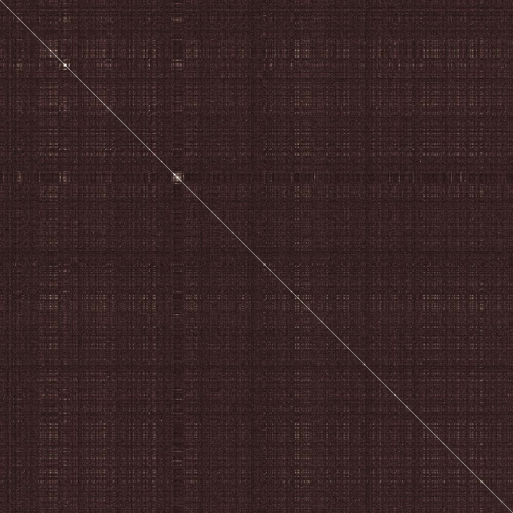
Distribution-clusters from a subset of Flickr11k [43]
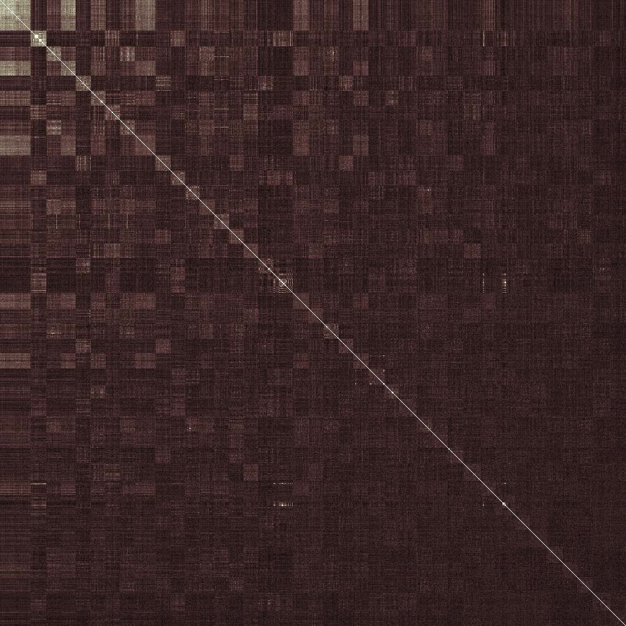Affinity matrix before and after clustering

Figure 1: Distribution-clustering on a set of random images. Our technique captures even highly variable distributions like flowers and scenery. The post-clustering affinity matrix displays distinctive blocky patterns predicted by our theory.

Conventional wisdom suggests poor clustering performance is due to two intrinsic factors. a) Images are the product of a complex interplay of geometric, illumination and occlusion factors. These are seldom constant, causing even images of the same location to vary significantly from each other. The extreme variability makes clustering difficult. This can be understood mathematically as each image being an instance of some distribution. The variability causes image data-sets to be chaotic. Here, chaotic is defined as having distributions whose mean separation is significantly smaller than their standard deviation. Clustering chaotic data is ill-posed because data points of different distributions mingle. This can be alleviated by enhancing invariance with higher dimensional image descriptors. However, it leads to a second problem. b) As dimensions increase, “contrast-loss” [3, 10, 17] occurs. Distances between points tend to a constant, with traditional clustering metrics becoming ill-defined [3, 5]. This is considered part of the curse of dimensionality [17, 1].

We offer a different perspective in which “contrast-loss” is not a problem but the solution to clustering chaotic data. The core idea is simple. What was previously interpreted as “contrast-loss” is actually the law of large numbers causing instances of a distribution to concentrate on a thin “hyper-shell”. The hollow shells mean data points from apparently overlapping distributions do not actually mingle, making choatic data intrinsically separable. We encapsulate this constraint into a second order cost that treats the rows of an affinity matrix as identifiers for instances of the same distribution. We term this distribution-clustering.

Distribution-clustering is fundamentally different from traditional clustering as it can disambiguate chaotic data, self-determine the number of clusters and is intrinsically robust to “outliers” that form their own clusters. This mind-bending result provides an elegant solution to a problem previously deemed intractable. Thus, we feel it fair to conclude that “contrast-loss” is a blessing rather than a curse.

1.1 Related Works

To date, there are a wide variety of clustering algorithms [32, 26, 19, 15, 21, 38] customized to various tasks. A comprehensive survey is provided in [9, 42]. Despite the variety, we believe distribution-clustering is the first to utilize the peculiarities of high dimensional space. The result in a fundamentally different clustering algorithm.

This work is also part of on-going research in the properties of high dimensional space. Pioneering research began with Beyer et al.’s [10] discovery of “contrast-loss”. This was interpreted as an intrinsic hindrance to clustering and machine learning [3, 10, 17], motivating the development of sub-space clustering [35, 18], projective-clustering [2, 27], and other techniques  [44, 28, 20] for alleviating “contrast-loss”. This simplistic view has begun to change, with recent papers observing that “contrast-loss” can be beneficial in detecting outliers [37, 47], cluster centroids [40] and scoring clusters [40]. These results indicate a gap in our knowledge but a high-level synthesis is still lacking.

While we do not agree with Aggarwal et al.’s [3] interpretation of “contrast-loss”, we are inspired by their attempts to develop a general intuition about the behavior of algorithms in high-dimensional space. This motivates us to analyze the problem from both intuitive and mathematical perspectives. We hope it contributes to the general understanding of high dimensional space.

Within the larger context of artificial intelligence research, our work can be considered research on similarity functions surveyed by Cha [13]. Unlike most other similarity functions, ours is statistical in nature, relying on extreme improbability of events to achieve separability. Such statistical similarity has been used both explicitly [11] and implicitly [30, 14, 36, 46, 39] in matching and retrieval. Many of these problems may be reformulatable in terms of the law of large numbers, “contrast-loss” and high-dimensional features. This is a fascinating and as yet unaddressed question.

Finally, distribution-clustering builds on decades of research on image descriptors [33, 25, 6] and normalization [24, 7]. These works reduce variation, making the law of large numbers more impactful at lower dimensions. As distribution-clustering is based on the law of large numbers, its performance is correspondingly enhanced.

2 Visualizing High Dimensions

Our intuition about space was formed in two and three dimensions and is often misleading in high dimensions. In fact, it can be argued that the “contrast-loss” curse ultimately derives from misleading visualization. This section aims to correct that.

At low dimensions, our intuition is that solids with similar parameters have significant volumetric overlap. This is not true in high dimensions.

Consider two high dimensional hyper-spheres which are identical except for a small difference in radius. Their volume ratio is

$$\left(\frac{r-\Delta r}{r}\right)^{k}=\left(1-\frac{\Delta r}{r}\right)^{k}\to 0,\quad k\to\infty$$ (1)

which tends to zero as the number of dimensions, $k\to\infty$. This implies almost all of a sphere’s volume is concentrated at its surface. Thus, small changes in either radius or centroid cause apparently overlapping spheres to have near zero intersecting volume as illustrated in Fig. 2, i.e., they become volumetrically separable! A more rigorous proof can be found in [23].

Figure 2: Almost all of a high dimensional sphere’s volume is near its surface. Thus, small changes of radius or centroid result in almost no volumetric overlap. The apparently overlapping spheres are volumetrically separable!

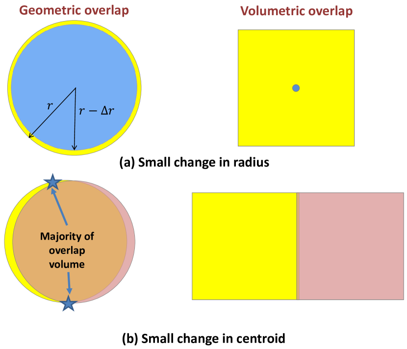
Intriguingly, instances of a distribution behave similarly to a hyper-sphere’s volume. Section 3.3 shows that when distributions have many independent dimensions, their instances concentrate on thin “hyper-shells”. Thus, instances of apparently overlapping distributions almost never mingle. This makes clustering chaotic data by distribution a well-posed problem, as illustrated in Fig. 3.

Figure 3: Left: Traditional view of chaotic data as overlapping spheres. Clustering such data is deemed an ill-posed problem. Right: Our visualization. Each distribution’s instances form hollow rings. Thus, clustering data by fitting “hyper-shells” becomes a well-posed problem.

3 Distribution-Clustering (theory)

Images are often represented as high dimensional feature vectors, such as the $4096$-dimensional NetVLAD [6] descriptor. This section shows how we can create indicators to group images based on their generative distributions.

Definition 1.

• $D(m,\sigma^{2})$ denotes a probability distribution with mean $m$ and variance $\sigma^{2}$ ;

• $\mathcal{S}_{n}=\{\begin{array}[]{cccc}1,&2,&\ldots,n\end{array}\}$ denotes a set of consecutive positive integers from $1$ to $n$;

• $d(.)$ denotes a normalized squared $\ell_{2}$ norm operator, i.e., for $\mathbf{x}\in\mathbb{R}^{k}$, $d(\mathbf{x})=\frac{\|\mathbf{x}\|^{2}}{k}$.

Let $\mathbf{Z}=\left[\begin{array}[]{cccc}Z_{1},&Z_{2},&\ldots,&Z_{k}\end{array}\right]^{T}$ denote a $k$ dimensional random vector where $Z_{i}$ is a random variable,

• $d(.)$ operator can also be applied on a random vectors $\mathbf{Z}$. $d(\mathbf{Z})=\frac{\|\mathbf{Z}\|^{2}}{k}$ is a random variable formed by averaging $\mathbf{Z}$’s squared elements.

• $E(\mathbf{Z})=\left[\begin{array}[]{cccc}\mathrm{E}(Z_{1}),&\mathrm{E}(Z_{2}),&\ldots,&\mathrm{E}(Z_{k})\end{array}\right]^{T}$ is a vector of each dimension’s expectation;

• With a slight abuse of notation, we define $\mathrm{Var}(\mathbf{Z})=\sum_{i=1}^{k}\frac{\mathrm{var}(Z_{i})}{k}$, as the average variance over all dimensions.

3.1 Passive Sensing Model

Many data sources (like cameras) can be modeled as passive sensors. Data points (like image descriptors) $\{\mathbf{x}^{(i)}:i\in\mathcal{S}_{n}\}$, are instances of random vectors $\{\mathbf{X}^{(i)}:i\in\mathcal{S}_{n}\}$ representing environmental factors that influence sensory outcome, e.g., camera position, time of day, weather conditions. As sensing does not influence the environment, all random vectors are mutually independent. Our goal is to cluster $\mathbf{x}^{(i)}$ instances by their underlying $\mathbf{X}^{(i)}$ distributions.

3.2 Quasi-ideal Features

An ideal feature descriptor has statistically independent dimensions. However, this is hard to ensure in practice. A more practical assumption is the quasi-independence in condition 1.

Condition 1.

Quasi-independent: A set of $k$ random variables $\{X^{(i)}:i\in\mathcal{S}_{k}\}$ are quasi-independent, if and only if, as $k\to\infty$, each random variable has finite number of pairwise dependencies. That is, let $\mathcal{A}$ be the set of all pairwise dependent variables and $\mathbf{1}$ be an indicator function, there exists $t\in\mathbb{Z}^{+}$ such that

$$\sum_{j=1}^{k}\mathbf{1}_{\mathcal{A}}(\{X^{(i)},X^{(j)}\})\leq t,\quad\forall i\in\mathcal{S}_{k}.$$

Quasi-independence is approximately equivalent to requiring information increases proportionally with number of random variables. When the random variables are concatenated into a feature, we term it quasi-ideal.

Condition 2.

Quasi-ideal: A $k$-dimensional random vector $\mathbf{X}$ is quasi-ideal, if and only if, as $k\to\infty$, the variance of all its elements are finite and the set of all its elements, $\{X_{i}:i\in\mathcal{S}_{k}\}$, is quasi-independent.

Treating the links of an infinitely long Markov chain as feature dimensions would create a quasi-ideal feature. This is useful in computer vision, as pixel values have Markov like properties of some statistical dependence on neighbors but long range statistical independence. Hence, many image based descriptors can be modeled as quasi-ideal.

Practicality aside, quasi-ideal features have useful mathematical properties, as they permit the law of large numbers to apply to distance metrics. This leads to interesting results summarized in Lemmas 1 and 2.

Lemma 1.

Let $\mathbf{X}$ be a quasi-ideal random vector with dimension $k\to\infty$. The normalized squared $\ell_{2}$ norm of any instance is almost surely a constant:

$$d(\mathbf{X})=\frac{\|\mathbf{X}\|^{2}}{k}=\frac{\sum_{i=1}^{k}X_{i}^{2}}{k}\sim D\left(m,\sigma^{2}\right),\sigma\to 0,$$ (2)

Proof.

As $\mathbf{X}$ is quasi-ideal, the set of squared elements $\{X_{1}^{2},X_{2}^{2},\ldots,X_{k}^{2}\}$ form a covariance matrix where the sum of elements in any row is bounded by some positive real number $t$, i.e.,

$$\sum_{j=1}^{k}\mathrm{cov}(X_{i}^{2},X_{j}^{2})\leq t,\quad\forall i\in\mathcal{S}_{k}.$$ (3)

This implies

$$\mathrm{Var}(d(\mathbf{X}))=\frac{\sum_{i=1}^{k}\sum_{j=1}^{k}\mathrm{cov}(X_{i}^{2},X_{j}^{2})}{k^{2}}<\frac{kt}{k^{2}}<\frac{t}{k}.$$ (4)

Thus, as $k\to\infty$, variance tends to zero. ∎

Lemma 2.

Let $\mathbf{X}$ and $\mathbf{Y}$ be statistically independent, quasi-ideal random vectors. As the dimensions $k\to\infty$.

$$d(\mathbf{X}-\mathbf{Y})=\frac{\|\mathbf{X}-\mathbf{Y}\|^{2}}{k}\sim D\left(m,\sigma^{2}\right),\sigma\to 0,$$ (5)

where $m=\mathrm{Var}(\mathbf{X})+\mathrm{Var}(\mathbf{Y})+d(\mathrm{E}(\mathbf{X})-\mathrm{E}(\mathbf{Y})).$

Proof.

As $\mathbf{X}$ and $\mathbf{Y}$ are quasi-ideal, random vector $\mathbf{X}-\mathbf{Y}$ is also quasi-ideal. Using Lemma 1, we know $d(\mathbf{X}-\mathbf{Y})$’s variance tends to zero. The expression for its mean is:

$$m= \mathrm{E}\left(\frac{\|\mathbf{X}-\mathbf{Y}\|^{2}}{k}\right)$$

$$= \sum_{i=1}^{k}\frac{\mathrm{E}\left(X_{i}^{2}\right)}{k}+\frac{\mathrm{E}\left(Y_{i}^{2}\right)}{k}-\frac{2\mathrm{E}\left(X_{i}Y_{i}\right)}{k}$$

$$= \sum_{i=1}^{k}\frac{\mathrm{var}\left(X_{i}\right)+\mathrm{var}\left(Y_{i}\right)}{k}$$

$$+\sum_{i=1}^{k}\frac{\mathrm{E}\left(X_{i}\right)^{2}-2\mathrm{E}\left(X_{i}\right)\mathrm{E}\left(Y_{i}\right)+\mathrm{E}\left(Y_{i}\right)^{2}}{k}$$

$$= \mathrm{Var}(\mathbf{X})+\mathrm{Var}(\mathbf{Y})+\sum_{i=1}^{k}\frac{\left(\mathrm{E}\left(X_{i}\right)-\mathrm{E}\left(Y_{i}\right)\right)^{2}}{k}$$

$$= \mathrm{Var}(\mathbf{X})+\mathrm{Var}(\mathbf{Y})+d(\mathrm{E}(\mathbf{X})-\mathrm{E}(\mathbf{Y})).$$

∎

Lemma 2 is similar in spirit to Beyer et al.’s [10] “contrast-loss” proof. However, it accommodates realizations from different distributions, introduces a more practical quasi-independence assumption and is simpler to derive.

Unlike [3], we consider “contrast-loss” an opportunity not a liability. Lemma 2 proves that distance between instances almost always depend only on the mean and variances of the underlying distributions and not on instances’ values. This makes distance between instances a potential proxy for identifying their underlying distributions.

3.3 Distribution-clusters

Identifying data points from “similar” distributions requires a definition of “similarity”. Ideally, we would follow Lemma 2’s intuition and define “similarity” as having the same mean and average variance. However, the definition needs to accommodate dimensions tending to infinity. This leads to a distribution-cluster based “similarity” definition.

Let $\Omega_{\mathbf{X}}=\{\mathbf{X}^{(i)}:i\in\mathcal{S}_{n}\}$ be a set of independent $k$-dimensional random vectors. $k\to\infty$ such that the random vectors satisfy quasi-ideal conditions.

Condition 3.

Distribution-cluster: $\Omega_{\mathbf{X}}$ forms a distribution-cluster if and only if:

• The normalized squared $\ell_{2}$ norm distance between any two distribution mean is zero, i.e.,

  $$d(\mathrm{E}(\mathbf{X}^{(i)})-\mathrm{E}(\mathbf{X}^{(j)}))=0,\quad\forall i,j\in\mathcal{S}_{n};\\$$ (6)

• All distributions have the same average variance, i.e.,

  $$\mathrm{Var}(\mathbf{X}^{(i)})=\mathrm{Var}(\mathbf{X}^{(j)}),\quad\forall i,j\in\mathcal{S}_{n}.$$ (7)

As dimensions tend to infinity, instances of a distribution-cluster concentrate on a “thin-shell”. This is proved in theorem 1 and validates Fig. 3’s intuition. The “hollow-center” means data points from apparently overlapping distributions almost never mingle, creating the potential for clustering chaotic data.

Theorem 1.

If $\Omega_{\mathbf{X}}$ is a distribution-cluster with average variance $v$, the normalized squared distance of its instances from the cluster centroid will almost surely be $v$, i.e., $\Omega_{\mathbf{X}}$’s instances form a thin annulus about it’s centroid.

Proof.

Without loss of generality, let $\mathbf{m}=E(\mathbf{X}^{(1)})$. Let $\mathbf{X}$ in Lemma 2 be $\mathbf{X}^{(i)}$ and $\mathbf{Y}$ in Lemma 2 be a distribution with mean $\mathbf{m}$ and variance $0$. This gives an expression:

$$p\left(d(\mathbf{X}^{(i)}-\mathbf{m})=v\right)\to 1\quad\forall i\in\mathcal{S}_{n}$$ (8)

∎

3.4 Grouping Data by Distribution

We seek to group a set of data points by their underlying distribution-clusters. This is achieved by proving that data points of a distribution-cluster share unique identifiers that we term cluster-indicators.

Theorem 2.

Cluster-indicator: Let $\mathbf{Y}$ be a quasi-ideal random vector that is independent of all $\Omega_{\mathbf{X}}$’s random vectors.

$\Omega_{\mathbf{X}}$ forms a distribution-cluster (c.f condition 3), if and only if, for any valid random vector $\mathbf{Y}$, there exists a real number $b_{\mathbf{Y}}$ such that

$$\begin{split}p(d(\mathbf{Y}-\mathbf{X}^{(i)})=b_{\mathbf{Y}})\to 1,\quad\forall i\in\mathcal{S}_{n}.\end{split}$$ (9)

Proof.

First, the if part is proved. Given $\Omega_{\mathbf{X}}$ is a distribution-cluster, Eq. (9) is a direct result of Lemma 2, where the distance between instances of quasi-ideal distributions are almost surely determined by the distributions’ mean and average variances.

Moving on to the only if proof, where it is given that $\Omega_{\mathbf{X}}$ satisfies Eq. (9)’s cluster-indicator. W.l.o.g, we consider only elements $\mathbf{X}^{(1)},\mathbf{X}^{(2)}$. Let $\mathbf{Y}$ be independent but identically distributed with $\mathbf{X}^{(1)}$.

From Lemma 2, we know that

• $p(d(\mathbf{Y}-\mathbf{X}^{(1)})=m_{1})\to 1,$ where

  $m_{1}=2\mathrm{Var}(\mathbf{X}^{(1)});$

• $p(d(\mathbf{Y}-\mathbf{X}^{(2)})=m_{2})\to 1,$ where

  $$m_{2}=\mathrm{Var}(\mathbf{X}^{(1)})+\mathrm{Var}(\mathbf{X}^{(2)})+d(\mathrm{E}(\mathbf{X}^{(1)})-\mathrm{E}(\mathbf{X}^{(2)})).$$

Equation (9) means $b_{\mathbf{Y}}=m_{1}=m_{2}$, implying:

$$\begin{split}&2\mathrm{Var}(\mathbf{X}^{(1)})\\ =&\mathrm{Var}(\mathbf{X}^{(1)})+\mathrm{Var}(\mathbf{X}^{(2)})+d(\mathrm{E}(\mathbf{X}^{(1)})-\mathrm{E}(\mathbf{X}^{(2)})).\end{split}$$ (10)

Similarly, treating $\mathbf{Y}$ as independent but identically distributed with $\mathbf{X}^{(2)}$ implies

$$\begin{split}&2\mathrm{Var}(\mathbf{X}^{(2)})\\ =&\mathrm{Var}(\mathbf{X}^{(1)})+\mathrm{Var}(\mathbf{X}^{(2)})+d(\mathrm{E}(\mathbf{X}^{(1)})-\mathrm{E}(\mathbf{X}^{(2)})).\end{split}$$ (11)

Solving (10) and (11) yields

$$\mathrm{Var}(\mathbf{X}^{(1)})=\mathrm{Var}(\mathbf{X}^{(2)}),\quad d(\mathrm{E}(\mathbf{X}^{(1)})-\mathrm{E}(\mathbf{X}^{(2)}))=0.$$

This proves that $\mathbf{X}^{(1)},\mathbf{X}^{(2)}$ are members of a distribution-cluster, (c.f condition 3). Repeating the process with all element pairs of $\Omega_{\mathbf{X}}$ will show they belong to one distribution-cluster. This completes the only if proof.

∎

As argued in Sec. 3.1, image descriptors can be modeled as instances of independent, quasi-ideal random vectors, i.e., a set of image descriptors $\Omega_{\mathbf{x}}=\{\mathbf{x}^{(i)}:i\in\mathcal{S}_{n}\}$ can be considered instances of the respective random vectors in $\Omega_{\mathbf{X}}$. Theorem 2 implies that descriptors from the same distribution-cluster will (almost surely) be equi-distance to any other descriptor. Further, it is a unique property of descriptors from the same distribution-cluster. This allows descriptors to be unambiguously assigned to distribution-clusters. In summary, distribution-clustering of images (and other passive sensing data) is a well-posed problem, per the definition in McGraw-Hill dictionary of scientific and technical terms [34]:

• A solution exist. This follows from Theorem 2’s if condition where cluster-indicators almost surely (in practice it can be understood as surely) identify all data points of a distribution-cluster;

• A solution is unique. This follows from Theorem 2’s only if condition which means cluster-indicators almost never confuse data points of different distributions. This can also be understood as proving intrinsic separability of instances from different distribution-clusters;

• The solution’s behavior changes continuously with the initial conditions. The $b_{\mathbf{Y}}$ cluster-indicator in Eq. (9) vary continuously with the mean and average variance of the underlying distribution-cluster. This follows from Lemma 2’s expression for $b_{\mathbf{Y}}$.

4 Distribution-Clustering (practical)

Our goal is to use theorem 2’s cluster-indicators to group data points by their underlying distributions. From theorem 2, we know that if $\mathbf{x}^{(i)},\mathbf{x}^{(j)}$ are instances of the same distribution-cluster, the affinity matrix’s $i,j$ rows/ columns will be near identical. To exploit this, we define second order features as columns of the affinity matrix. Clustering is achieved by grouping second-order features.

4.1 Second-order Affinity

Let $\Omega_{\mathbf{x}}=\{\mathbf{x}^{(i)}:i\in{S}_{n}\}$ be a set of realizations, with an associated affinity matrix $\mathbf{A}_{n\times n}$:

$$\mathbf{A}(i,j)=d(\mathbf{x}^{(i)}-\mathbf{x}^{(j)}).$$ (12)

The columns of $\mathbf{A}$ are denoted as $\mathbf{a}^{(i)}=\mathbf{A}(:,i)$. Treating columns as features yields a set of second-order features $\{\mathbf{a}^{(i)}:i\in\mathcal{S}_{n}\}$. The elements of $\mathbf{a}^{(i)}$ encodes the distance between vector $\mathbf{x}^{(i)}$ and all others in $\Omega_{x}$.

From theorem 2, we know that if and only if the distributions underlying $\mathbf{a}^{(i)},\mathbf{a}^{(j)}$ come from the same distribution-cluster, all their elements, except the $i^{th}$ and $j^{th}$ entries, are almost surely identical. This is encapsulated as a second-order distance:

$$d^{\prime}(\mathbf{a}^{(i)},\mathbf{a}^{(j)})=\sum_{k\in\mathcal{S}_{n}\setminus\{i,j\}}\left(a^{(i)}_{k}-a^{(j)}_{k}\right)^{2}.$$ (13)

which should be zero if $i,j$ belong to the same distribution-cluster. The presence of clusters of identical rows causes the post-clustering affinity matrix to display a distinctive blocky pattern shown in Fig. 1.

Second order distance can be embedded in existing clustering algorithms. For techniques like spectral-clustering [45] which require an affinity matrix, a second-order affinity matrix is defined as $\mathbf{A}^{\prime}_{n\times n}$:

$$\mathbf{A}^{\prime}(i,j)=d^{\prime}\left(\mathbf{a}^{(i)},\mathbf{a}^{(j)}\right).$$

If $n$ is large, $d^{\prime}\left(\mathbf{a}^{(i)},\mathbf{a}^{(j)}\right)\approx\|\mathbf{a}^{(i)}-\mathbf{a}^{(j)}\|^{2}$. This allows second order $\{\mathbf{a}^{(i)}\}$ features to be used directly in clustering algorithms like k-means, which require feature inputs.

Incorporating second-order constraints into a prior clustering algorithm does not fully utilize theorem 2. This is because realizations of the same distribution-cluster have zero second-order-distance, while most clustering algorithms only apply a distance penalty. This motivates an alternative solution we term distribution-clustering

4.2 Implementing Distribution-clustering

Distribution-clustering can be understood as identifying indices whose mutual second-order distance is near zero. These are grouped into one cluster and the process repeated to identify more clusters.

An algorithmic overview is as follows. Let $i,j$ be the indices of its smallest off-diagonal entry of affinity matrix $\mathbf{A}$. If $\{\mathbf{x}^{(i)},\mathbf{x}^{(j)}\}$ are instances of a distribution-cluster, Lemma 2 states the average cluster variance is $\mathbf{A}(i,j)/2$. Thus they are the data-set’s lowest average variance distribution-cluster. Initialize $\{\mathbf{x}^{(i)},\mathbf{x}^{(j)}\}$ as a candidate distribution-cluster. New members are recruited by finding vectors whose average second-order distance from all distribution-cluster candidates is less than threshold $\tau$. If a candidate distribution-cluster grows to have no less than $m$ members, accept it. Irrespective of the outcome, remove $\{\mathbf{x}^{(i)},\mathbf{x}^{(j)}\}$ from consideration as candidate clusters. Repeat on un-clustered data till all data points are clustered or it is impossible to form a candidate cluster. Some data may not be accepted in any cluster and remain outliers. Details are in Algorithm 1. For whitened descriptors [24, 7], typical parameters are $\tau=0.07,m=5$.

Input: Affinity matrix $\mathbf{A}_{n\times n}$

Output: Vector of cluster labels $\mathbf{L}$

Initialization: 1) Set of un-assigned image indices: $\mathcal{S}_{n}=\{1,2,\ldots,n\}$;   2) Set of non-diagonal elements of $\mathbf{A}$: $\mathcal{E}=\{\mathbf{A}(i,j)\},i\neq j$;   3) Initialize $\mathbf{L}=\mathbf{0}_{n\times 1}$; 4) Set label counter $c=1$;

while $\mathcal{S}_{n}\neq\emptyset$ do

       Find $i$ and $j$ corresponding to $\min(\mathcal{E})$;

       Create candidate cluster $\mathcal{H}=\{i,j\}$;

       for $s\in\mathcal{S}_{n}$ do

             if $\frac{1}{|\mathcal{H}|}\sum_{h\in\mathcal{H}}d^{\prime}(\mathbf{a}^{(s)},\mathbf{a}^{(h)})<\tau$, then

                   insert $s$ into $\mathcal{H}$

             end if

            

       end for

      if $|\mathcal{H}|<$ m then

             delete $\mathbf{A}(i,j)$ from $\mathcal{E}$ ;

            

      else

             accept cluster $\mathcal{H}$ and assign its elements a unique label;

             $\mathbf{L}(h)=c,\;\;\;\;\forall h\in\mathcal{H}$;

             $c:=c+1$;

            

            for $h\in\mathcal{H}$  do

                   delete $\mathbf{A}(:,h)$ and $\mathbf{A}(h,:)$ from set $\mathcal{E}$;

                   delete $h$ from set $\mathcal{S}_{n}$.

             end for

            

       end if

      

end while

Algorithm 1 Distribution-clustering

Relative to other clustering techniques, distribution-clustering has many theoretical and practical advantages:

• Clustering chaotic data is a well-posed problem (c.f. Sec. 3.4);

• No pre-definition of cluster numbers is required;

• Innate robustness to “outliers” which form their own clusters.

5 Clustering

Simulation Results

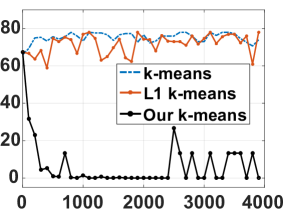
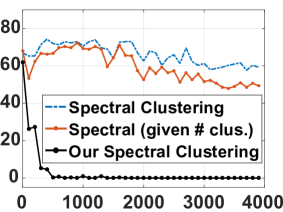
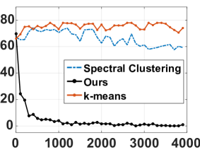
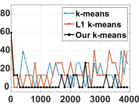
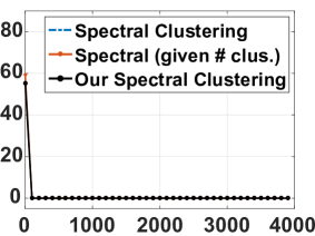
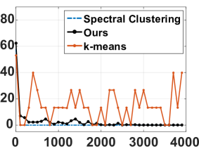
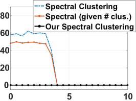
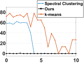
use quasi-ideal features created from a mixture of uniform and Gaussian distributions. To evaluate the effect of increasing dimensionality, the number of dimensions is increased from $1$ to $4000$. Two sets are evaluated. The “Easy” set has wide separation of underlying distributions while the “Difficult” set has little separation. Results are presented in Fig. 4. We compare three different distance measures on k-means clustering [31, 8]: $\ell_{2}$ norm, $\ell_{1}$ norm and our proposed second-order distance in Eq. (13). We also compare spectral clustering [45] with $\ell_{2}$ and second-order distance. Finally, we provide a system to system comparison between our distribution-clustering, k-means and spectral-clustering. At low dimensions, the second-order distance gives results comparable to other algorithms. However, performance steadily improves with number of dimensions. Notably, only algorithms which employ second-order distance are effective on the “Difficult” set. This validates the theoretical prediction that (the previously ill-posed problem of) clustering chaotic data is made well-posed by the second-order distance.

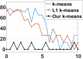
To study the effect of mean separation on clustering performance, we repeat the previous experiment under similar conditions, except the number of dimensions are kept constant and the mean separation progressively reduced to zero. Results are presented in Fig. 5. Note that second-order distance ensures clustering performance is relatively invariant to mean separation.

Difficult
Easy

Figure 4: Simulation with increasing number of dimensions. Left: k-means with $\ell_{2}$ norm, k-means with $\ell_{1}$ norm and our second-order distance. Center: Spectral clustering with automatic detection of cluster numbers [45], given number of clusters [45] and second-order distance (Eq. (13)). Right: System to system comparison of distribution-clustering, k-means and spectral clustering. Only high dimensional, second-order distance algorithms are effective on “Difficult” data.

$\%$ Mis-classified vs. Separation of distribution centers

Figure 5: Simulation with increasing separation of distribution centers. Algorithms are the same as in Fig. 4. Only second-order distance algorithms are performance invariant with separation of distribution centers.

Real Images

with NetVLAD [6] as image descriptors are used to evaluate clustering on 5 data-sets: Handwritten numbers in Mnist [29]; A mixture of images from Google searches for “Osaka castle”’ and “Christ the redeemer statue”; 2 sets of 10 object types from CalTech 101 [22]; And a mixture of ImageNet [16] images from the Lion, Cat, Tiger classes. Distribution-clustering is evaluated against five baseline techniques: K-means  [31, 8], spectral-clustering [45], projective-clustering [4], GMM [12] and quick-shift [41]. For k-means and GMM, the number of clusters is derived from distribution-clustering. This is typically $20-200$. Spectral and projective-clustering are prohibitively slow with many clusters. Thus, their cluster numbers are fixed at $20$.

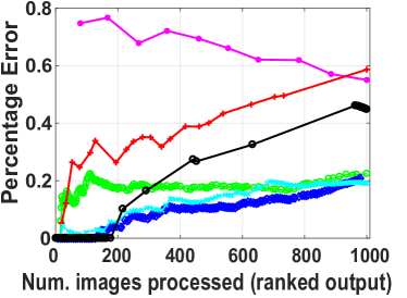
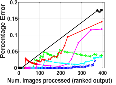
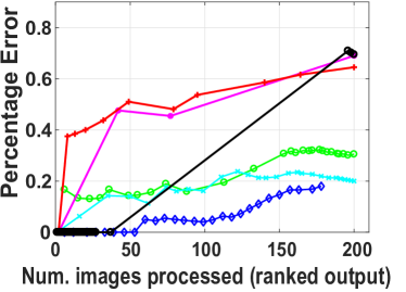
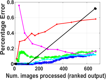
Cluster statistics are reported in Tab. 1. On standard silhouette and purity scores, distribution-clustering’s performance is comparable to benchmark techniques. The performance is decent for a new approach and validates Theorem 2’s “contrast-loss” constraint in the real-world. However, an interesting trend hides in the average statistics.

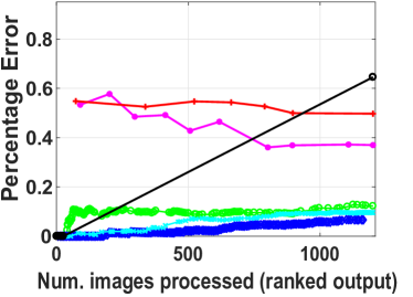
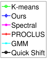
Breaking down the purity score to find the percentage of images deriving from pure clusters, i.e., clusters with no wrong elements, we find that distribution-clustering assigns a remarkable fraction of images to pure clusters. On average, it is $1.5$ times better than the next best algorithm and in some cases can nearly double the performance. This is important to data-abstraction where pure clusters allow a single average-feature to represent a set of features. In addition, distribution-clustering ensures pure clusters are readily identifiable. Figure 6 plots percentage error as clusters are processed in order of variance. Distribution-clustering keeps “outliers” packed into high-variance clusters, leaving low-variance clusters especially pure. This enables concepts like image “over-segmentation” to be transferred to unorganized image sets.

K-means and GMM are the closest alternative to distribution-clustering. However, their clusters are less pure and they are dependent on distribution-clustering to initialize the number of clusters. This makes distribution-clustering one of the few (only?) methods effective on highly chaotic image data like Flickr11k [43] demonstrated in Fig. 1.

Minst	Internet Images
CalTech101 (Set1)	CalTech101 (Set2)
Cats

Figure 6: Clustering real images. Clusters are ranked by variance. Unlike prior methods where “outliers” are randomly scattered in clusters, distribution-clustering concentrates “outliers” in high variance clusters, making identification of pure clusters easy.

	Silhouette Score
Dataset	K-Means	Spectral	PROCLUS	GMM	QS	Ours
	[31, 8]	[45]	[4]	[12]	[41]
MNIST	0.0082	0.0267	-0.0349	0.0076	0.0730	0.038
Internet	0.084	0.041	-0.038	0.0963	0.0488	0.003
CalTech1	0.027	0.02	-0.0045	0.0373	0.0999	0.074
CalTech2	0.028	0.084	-0.0186	0.0248	0.0350	0.042
Cats	0.007	0	-0.002	0.0236	0.0752	0.0239
Average	0.0308	0.034	-0.020	0.0379	0.0532	0.036
	Purity Score
Dataset	K-Means	Spectral	PROCLUS	GMM	QS	Ours
MNIST	0.77	0.45	0.41	0.81	0.55	0.79
Internet	0.96	0.90	0.86	0.97	0.82	0.97
CalTech1	0.71	0.44	0.36	0.80	0.31	0.82
CalTech2	0.84	0.83	0.41	0.88	0.29	0.87
Cats	0.88	0.63	0.50	0.90	0.35	0.93
Average	0.83	0.65	0.51	0.87	0.46	0.88
	$\%$ of images in pure clusters (excluding singletons)
Dataset	K-Means	Spectral	PROCLUS	GMM	QS	Ours
MNIST	0.28	0	0	0.32	0.059	0.49
Internet	0.83	0.82	0.40	0.83	0.031	0.92
CalTech1	0.08	0.02	0.01	0.30	0.081	0.52
CalTech2	0.47	0.24	0	0.52	0.16	0.65
Cats	0.34	0	0	0.40	0.017	0.72
Average	0.40	0.22	0.082	0.47	0.070	0.66
	$\%$ of pure clusters (excluding singletons)
Dataset	K-Means	Spectral	PROCLUS	GMM	QS	Ours
MNIST	0.43	0	0	0.44	0.62	0.49
Internet	0.80	0.90	0.8	0.83	0.40	0.93
CalTech1	0.30	0.20	0.09	0.46	0.75	0.52
CalTech2	0.54	0.20	0	0.57	0.67	0.67
Cats	0.57	0	0	0.55	0.50	0.74
Average	0.53	0.32	0.178	0.57	0.59	0.67

Table 1: Cluster Statistics. Distribution-clustering ensures a large percentage of images belong to pure clusters.

Timing

excludes feature extraction cost which is common to all algorithms. Experiments are on an i7 machine, with $4096$ dimension NetVlad [6] features computed over the $400$ images of Internet data-set. Our single core, Matlab implementation of distribution-clustering takes $23$ seconds, of which $4.5$ seconds was spent computing the affinity matrix. Timing for other algorithms are as follows. K-means [31, 8]: $0.73$ seconds, Quick Shift [41] (Python): $1.5$ seconds, spectral clustering [45] (20 clusters): $2$ seconds, GMM [12]: $4$ minutes and PROCLUS [4] (20 clusters on OpenSubspace V3.31): 9 minutes.

Qualitative

inspection of distribution-clusters show they have a purity not captured by quantitative evaluation. Figure 7 illustrates this on Colosseum images crawled from the web. Quantitatively, both distribution-clustering and k-means are nearly equal, with few clusters mixing Colosseum and “outlier” images. However, distribution-clusters are qualitatively better, with images in a cluster sharing a clear, generative distribution.

Other

things readers may want to note. More qualitative evaluation of clustering is available in the supplementary. Code is available at http://www.kind-of-works.com/.

Distribution-clustering	K-means clustering

Figure 7: Distribution-clustering provides fine intra-cluster consistency, with images of a cluster sharing a clear, generative distribution. This qualitative improvement is not captured in evaluation statistics.

6 Conclusion

We have shown that chaotically overlapping distributions become intrinsically separable in high dimensional space and proposed a distribution-clustering algorithm to achieve it. By turning a former curse of dimensionality into a blessing, distribution-clustering is a powerful technique for discovering patterns and trends in raw data. This can impact a wide range of disciplines ranging from semi-supervised learning to bio-informatics.

References

- [1] https://en.wikipedia.org/wiki/Curse_of_dimensionality. Accessed: 2017-11-10.
- [2] P. K. Agarwal and N. H. Mustafa. K-means projective clustering. In Proceedings of ACM SIGMOD-SIGACT-SIGART symposium on Principles of Database Systems, pages 155–165, 2004.
- [3] C. C. Aggarwal, A. Hinneburg, and D. A. Keim. On the surprising behavior of distance metrics in high dimensional spaces. In Proceedings of International Conference on Database Theory (ICDT), volume 1, pages 420–434, 2001.
- [4] C. C. Aggarwal, J. L. Wolf, P. S. Yu, C. Procopiuc, and J. S. Park. Fast algorithms for projected clustering. In Proceedings of the ACM SIGMOD International Conference on Management of Data, number 2, pages 61–72, 1999.
- [5] C. C. Aggarwal and P. S. Yu. Outlier detection for high dimensional data. In Proceedings of the ACM SIGMOD International Conference on Management of Data, number 2, pages 37–46, 2001.
- [6] R. Arandjelovic, P. Gronat, A. Torii, T. Pajdla, and J. Sivic. Netvlad: CNN architecture for weakly supervised place recognition. In Proceedings of IEEE Conference on Computer Vision and Pattern Recognition (CVPR), pages 5297–5307, 2016.
- [7] R. Arandjelović and A. Zisserman. Three things everyone should know to improve object retrieval. In Proceedings of IEEE Conference on Computer Vision and Pattern Recognition (CVPR), pages 2911–2918, 2012.
- [8] D. Arthur and S. Vassilvitskii. k-means++: The advantages of careful seeding. In Proceedings of the eighteenth annual ACM-SIAM symposium on Discrete algorithms, pages 1027–1035, 2007.
- [9] P. Berkhin et al. A survey of clustering data mining techniques. Grouping Multidimensional Data, 25:71, 2006.
- [10] K. Beyer, J. Goldstein, R. Ramakrishnan, and U. Shaft. When is nearest neighbor meaningful? In Proceedings of International Conference on Database Theory (ICDT), pages 217–235, 1999.
- [11] J. Bian, W.-Y. Lin, Y. Matsushita, S.-K. Yeung, T.-D. Nguyen, and M.-M. Cheng. Gms: Grid-based motion statistics for fast, ultra-robust feature correspondence. In Proceedings of IEEE Conference on Computer Vision and Pattern Recognition (CVPR), pages 2828–2837, 2017.
- [12] C. Bishop. Pattern recognition and machine learning. Springer, 2007.
- [13] S.-H. Cha. Comprehensive survey on distance/similarity measures between probability density functions. International Journal of Mathematical Models and Methods in Applied Sciences, 1(300–307):1, 2007.
- [14] A. Delvinioti, H. Jégou, L. Amsaleg, and M. E. Houle. Image retrieval with reciprocal and shared nearest neighbors. In Proceedings of International Conference on Computer Vision Theory and Applications (VISAPP), volume 2, pages 321–328, 2014.
- [15] A. P. Dempster, N. M. Laird, and D. B. Rubin. Maximum likelihood from incomplete data via the em algorithm. Journal of the royal statistical society. Series B (methodological), pages 1–38, 1977.
- [16] J. Deng, W. Dong, R. Socher, L.-J. Li, K. Li, and L. Fei-Fei. Imagenet: A large-scale hierarchical image database. In Proceedings of IEEE Conference on Computer Vision and Pattern Recognition (CVPR), pages 248–255, 2009.
- [17] P. Domingos. A few useful things to know about machine learning. Communications of the ACM, 55(10):78–87, 2012.
- [18] E. Elhamifar and R. Vidal. Sparse subspace clustering: Algorithm, theory, and applications. IEEE Transactions on Pattern Analysis and Machine Intelligence, 35(11):2765–2781, 2013.
- [19] M. Ester, H.-P. Kriegel, J. Sander, X. Xu, et al. A density-based algorithm for discovering clusters in large spatial databases with noise. In Proceedings of ACM SIGKDD Conference on Knowledge Discovery and Data Mining, volume 96, pages 226–231, 1996.
- [20] D. Francois, V. Wertz, and M. Verleysen. The concentration of fractional distances. IEEE Transactions on Knowledge and Data Engineering, 19(7):873–886, 2007.
- [21] M. X. Goemans and D. P. Williamson. Improved approximation algorithms for maximum cut and satisfiability problems using semidefinite programming. Journal of the ACM (JACM), 42(6):1115–1145, 1995.
- [22] G. Griffin, A. Holub, and P. Perona. Caltech-256 object category dataset. 2007.
- [23] J. Hopcroft and R. Kannan. Foundations of data science. 2014.
- [24] H. Jégou and O. Chum. Negative evidences and co-occurences in image retrieval: The benefit of pca and whitening. Proceedings of European Conference on Computer Vision (ECCV), pages 774–787, 2012.
- [25] H. Jégou, M. Douze, C. Schmid, and P. Pérez. Aggregating local descriptors into a compact image representation. In Proceedings of IEEE Conference on Computer Vision and Pattern Recognition (CVPR), pages 3304–3311, 2010.
- [26] T. Kanungo, D. M. Mount, N. S. Netanyahu, C. D. Piatko, R. Silverman, and A. Y. Wu. An efficient k-means clustering algorithm: Analysis and implementation. IEEE Transactions on Pattern Analysis and Machine Intelligence, 24(7):881–892, 2002.
- [27] H.-P. Kriegel, P. Kröger, and A. Zimek. Clustering high-dimensional data: A survey on subspace clustering, pattern-based clustering, and correlation clustering. ACM Transactions on Knowledge Discovery from Data (TKDD), 3(1):1, 2009.
- [28] H.-P. Kriegel, A. Zimek, et al. Angle-based outlier detection in high-dimensional data. In Proceedings of ACM SIGKDD Conference on Knowledge Discovery and Data Mining, pages 444–452, 2008.
- [29] Y. LeCun, L. Bottou, Y. Bengio, and P. Haffner. Gradient-based learning applied to document recognition. Proceedings of the IEEE, 86(11):2278–2324, 1998.
- [30] W.-Y. Lin, S. Liu, N. Jiang, M. N. Do, P. Tan, and J. Lu. Repmatch: Robust feature matching and pose for reconstructing modern cities. In Proceedings of European Conference on Computer Vision (ECCV), pages 562–579, 2016.
- [31] S. P. Lloyd. Least squares quantization in pcm. IEEE Transactions on Information Theory, 28:129–137, 1982.
- [32] A. Y. Ng, M. I. Jordan, and Y. Weiss. On spectral clustering: Analysis and an algorithm. In Proceedings of Advances in Neural Information Processing Systems (NIPS), pages 849–856, 2002.
- [33] A. Oliva and A. Torralba. Modeling the shape of the scene: A holistic representation of the spatial envelope. International Journal of Computer Vision, 42(3):145–175, 2001.
- [34] S. P. Parker. McGraw-Hill dictionary of scientific and technical terms. McGraw-Hill, 1984.
- [35] L. Parsons, E. Haque, and H. Liu. Subspace clustering for high dimensional data: a review. ACM SIGKDD Explorations Newsletter, 6(1):90–105, 2004.
- [36] D. Qin, S. Gammeter, L. Bossard, T. Quack, and L. Van Gool. Hello neighbor: Accurate object retrieval with k-reciprocal nearest neighbors. In Proceedings of IEEE Conference on Computer Vision and Pattern Recognition (CVPR), pages 777–784, 2011.
- [37] M. Radovanović, A. Nanopoulos, and M. Ivanović. Reverse nearest neighbors in unsupervised distance-based outlier detection. IEEE transactions on Knowledge and Data Engineering, 27(5):1369–1382, 2015.
- [38] J. Shi and J. Malik. Normalized cuts and image segmentation. IEEE Transactions on Pattern Analysis and Machine Intelligence, 22(8):888–905, 2000.
- [39] M. Shi, Y. Avrithis, and H. Jégou. Early burst detection for memory-efficient image retrieval. In Proceedings of IEEE Conference on Computer Vision and Pattern Recognition (CVPR), pages 605–613, 2015.
- [40] N. Tomasev, M. Radovanovic, D. Mladenic, and M. Ivanovic. The role of hubness in clustering high-dimensional data. IEEE Transactions on Knowledge and Data Engineering, 26(3):739–751, 2014.
- [41] A. Vedaldi and S. Soatto. Quick shift and kernel methods for mode seeking. Proceedings of European Conference on Computer Vision (ECCV), 2008.
- [42] D. Xu and Y. Tian. A comprehensive survey of clustering algorithms. Annals of Data Science, 2(2):165–193, 2015.
- [43] Y. H. Yang, P. T. Wu, C. W. Lee, K. H. Lin, W. H. Hsu, and H. H. Chen. Contextseer: context search and recommendation at query time for shared consumer photos. In Proceedings of ACM international conference on Multimedia, pages 199–208, 2008.
- [44] D. Yu, X. Yu, and A. Wu. Making the nearest neighbor meaningful for time series classification. In Proceedings of International Congress on Image and Signal Processing, pages 2481–2485, 2011.
- [45] L. Zelnik-Manor and P. Perona. Self-tuning spectral clustering. In Proceedings of Advances in Neural Information Processing Systems (NIPS), pages 1601–1608, 2005.
- [46] S. Zhang, M. Yang, T. Cour, K. Yu, and D. N. Metaxas. Query specific fusion for image retrieval. In Proceedings of European Conference on Computer Vision (ECCV), pages 660–673. 2012.
- [47] A. Zimek, E. Schubert, and H.-P. Kriegel. A survey on unsupervised outlier detection in high-dimensional numerical data. Statistical Analysis and Data Mining: The ASA Data Science Journal, 5(5):363–387, 2012.