Do long-cadence data of the Kepler satellite capture basic properties of flares ?

Abstract

Flare research is becoming a burgeoning realm in the study of stellar activity due to the launch of Kepler in 2009. Kepler provides data with two time resolutions, i.e., the long-cadence (LC) data with a time resolution of 30 minutes and the short-cadence(SC) data with a time resolution of 1 minute, both of which can be used to study stellar flares. In this paper, we search flares in light curves with both LC data and SC data, and compare them in aspects of the true-flare rate, the flare energy, the flare amplitude, and the flare duration. It is found that LC data systematically underestimated the energies of flares by 25%, and underestimated the amplitudes of flares by 60% compared with SC flares. The duration are systematically overestimated by 50% compared with SC flares. However, the above percentages are poorly constrained and there is a lot of scatter. About 60% SC flares have not been detected by LC data. We investigate the limitation of LC data, and suggest that although LC data cannot reflect the detailed profiles of flares, they also can capture the basic properties of stellar flares.

1. INTRODUCTION

The Kepler satellite (Borucki et al., 2010) has yielded the light curves of more than 200,000 stars with unprecedented precision up to 17 quarters of continuous observations. Its precision for bright targets (V = 9-10) approaches 10 ppm, and 100 ppm for fainter targets(V = 13-14). It thus has ushered in a new era of stellar photometric investigation. Using the data of Kepler mission to study the property of the flare can reveal many very important aspects of stellar physics, such as stellar activity, the mechanism of superflares, stellar structure, the interaction of binary and so on (e.g., Shibayama et al., 2013; Balona, 2013; Hawley et al., 2014; Gaulme et al., 2014; Wichmann et al., 2014; Balona, 2015; Lurie et al., 2015; Davenport, 2016; Gao et al., 2016; Chang et al., 2017; Van Doorsselaere et al., 2017; Yang et al., 2017).

Kepler supplies two kinds of data with different time resolution, i.e., the long-cadence (LC) data with a time resolution of 30 minutes and the short-cadence(SC) data with a time resolution of 1 minute sampling interval. As known on our sun, most flares are microflares and nanoflares, which last for several minutes (e.g., Benz & Güdel, 2010). LC flares often have longer duration and much more energies. Most of them thus are superflares with a low resolution.

Obviously, SC data are more suitable for studying flares. However, there are only about 5000 sources with SC data, and usually with rather short time coverage (about two months on average). Therefore, some work began to use LC data to study flares (e.g., Walkowicz et al., 2011; Shibayama et al., 2013; Davenport, 2016; Gao et al., 2016; Yang et al., 2017), although deviations and errors of the data, such as the estimations for the energies, the durations, the amplitudes, and the true-flare rate, are not known accurately.

The differences between LC flares and SC flares may be underestimated by previous works. For example, Shibayama et al. (2013) compared two flares both in LC and SC data, and obtained a good consistency of them. Then they concluded that the flare energies estimated from LC data and SC data were similar. However, only two examples are not enough to indicate the correspondence of LC flares and SC flares. Actually, flares of LC and SC data may be much different. Issues such as the misaligned peak, the profile and the flare number can result in large deviations, which will be discussed in this work.

Hawley et al. (2014) suggested that, in SC data, the flattening tendency of the flare frequency distribution (FFD) is not due to detection limit but a real feature. On the other hand, Yang et al. (2017) compared the FFD between LC and SC data, and found that the flattening tendency of LC data is due to detection limit.

Balona (2012, 2013) reported flares detected in A-type stars. This discovery has raised a big challenge to the dynamo theory, because these stars are traditionally considered without significant convective envelopes. However, only LC are observed for most of those stars, and a large fraction of flares in those LC data are unresolved. Pedersen et al. (2017) presented detailed analyses of those stars and found more than half of them are subject to contaminations. It raises the question whether the analysis of flares by LC data is reliable, given its low time resolution as compared to SC data, which we believe can capture the detailed properties of flares. To answer the above question, a strict comparison of flares both in LC and SC data is essential.

Since there are many interesting results available on flares that either support or challenge the traditional theories, it is necessary to conduct an elaborate study on Kepler data. In this work, we explore the relation of the flares between LC and SC data, and carry out statistical comparison on their energies, durations and amplitudes. We try to give quantized indices to describe deviations and errors of LC flares, and search for conditions where flares can be studied with LC data. In Section 2, we introduce the data used and describe the method of analysis. In Section 3, the main results and the statistical analyses are presented and discussed. We present our conclusions in Section 4.

2. Data and Method

Figure 1.— Examples of flare searching in LC and SC data within the same time range. The top panel and bottom panel corresponds the LC and SC observations respectively. The horizontal axis is the Kepler Barycentric Julian Day (BKJD) (BJD$-$2454833) and the vertical axis is the relative flux (ppm). The black points are the observed stellar flux, the blue line are baselines, and the red lines mark the flare candidates.

2.1. LC and SC Data

In the Kepler data, a set of coadded and stored pixels obtained at a specific time is referred to as a cadence, and the total amount of time over which the data in a cadence is coadded is the cadence period. The two cadence periods in use are LC and SC. Each cadence consists of a series of frames that each includes a 6.02 s exposure time and a 0.52 s readout time. For LC data and Full Frame Images (FFI), 270 frames are coadded, leading to a total of 1765.5 s = 0.4904 h. For SC data, 9 frames are coadded, leading a total of 58.85 s (Van Cleve & Caldwell, 2009).

Our work is based on the entire Kepler mission data set (Q1-Q17; 48 months; Data Release 25). Kepler provides uncorrected simple aperture photometry (SAP) and pre-search data conditioning (PDC) in which instrumental effects are removed. However, PDC data could also remove some outliers that may be flare peaks. Therefore, SAP data are utilized in our research, as is done in Balona (2015) and Davenport (2016).

In total, there are 5140 targets in Kepler data with SC observations. All of the time segments of SC data are also covered by the LC data, i.e, all of SC data have their corresponding LC data with the same time coverage. The flare search is carried out in overlaps of LC and SC data.

2.2. Flare detection and Energy Estimation

The methods of flare detection and energy estimation are the same as those used in Yang et al. (2017) and we refer the interested readers to this reference for a detailed description. Here, we only present the main steps to detect flares: (1) To fit the baseline with an appropriate median filter. An iterative $\sigma$-clipping approach is applied to remove possible flares before fitting the continuum. (2) All outliers of LC data above $3\sigma$ against the baseline are marked as flare candidates, while in SC data, outliers with no less than three consecutive points are defined as flare candidates.

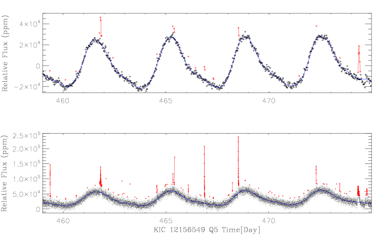
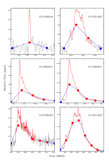
Figure 1 illustrates the flare detection, and gives a comparison of flare candidates between LC and SC data. It could be inferred that amplitudes of the flares with different time resolution are not correlated well. Many small LC flares show high amplitudes in SC data. Most of the isolated outliers with only one point of LC data are artifacts, while a few of them correspond true flares in SC data.

For a detailed description of our approach for the energy estimation, the readers are referred to Shibayama et al. (2013) and Yang et al. (2017). Its main principles are as follows: (1) The white light flare can be described by a black-body radiation model with the effective temperature of 9000 K. (2) The flare area can be calculated by flare amplitude, stellar radius, stellar effective temperature and Kepler response function.

Figure 2.— Examples of various artificial flares in LC (top) and SC (middle and bottom) data. The black line are the detrended flux. The red lines are the false positive flares. The top left panel shows the artifact caused by discontinuity. The top right panel shows the abnormally low points, which could cause their nearby points to be higher than $3\sigma$. The middle left panel shows the symmetrical profile of a flare candidate, which is removed in our sample. The middle right panel shows the periodically impulsive signals in Q2. The bottom panels show the false positive signals that appear in the Kepler records for many stars at the same time segments.

2.3. What is a True Flare?

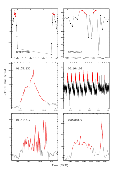
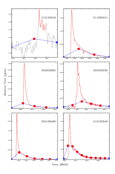
For most flares, the time resolution of LC data is low, of which even an isolated outlier may be a true flare. The time resolution of SC data is enough. However, flares in SC data could also be unreliable. For example, Figure 2 shows various false-positive signals in SC and LC data. A symmetric profile (middle left panel), a periodically impulsive artifact (middle right panel), or even missing data could cause false-positive signals, which imply instrumental errors or other artifacts.

As our purpose is to compare flares of LC and SC data, here, we stipulate that a true flare need to meet three basic criteria:

(1) In LC and SC data, the corresponding flares should occur at the same time within a window of half an hour.

(2) The SC flare should have at least three consecutive points, which are 3$\sigma$ above the baseline and is fully resolved.

(3) The profile of flares in SC data should have an impulsive rise and an exponential decay, i.e., the decay duration should be longer than the rise duration. For instance, the middle left panel of Figure 2 shows the example of a symmetric flare candidate. It should be noted that a lot of solar flares may have shapes that differ from the assumed profile.

Table 1 Time segments containing discontinuities or abnormal low points.

Quarter	Begin Time	End Time	Begin Time	End Time
	(Day)	(Day)	(Day)	(Day)
Q2	250.80	251.00	–	–
Q3	333.30	333.50	342.50	342.90
Q7	633.70	634.30	644.20	644.50
Q7	659.10	659.15	–	–
Q8	737.30	737.60	740.40	740.45
Q9	850.20	850.40	929.50	929.80
Q10	946.00	946.30	–	–
Q11	1003.20	1004.60	1008.20	1008.50
Q11	1021.30	1021.50	–	–
Q14	1278.50	1278.70	–	–

• Notes: Instrumental errors are numerous and pervasive in the above time segments. All the flare candidates in them are removed from our sample.

We emphasize that the purpose of the above three criteria is mainly to filter out artifacts rather than to identify true flares. In fact, there are various artifacts in the Kepler data that meet all the three criteria above. For example, the top panels of Figure 2 show the artifacts caused by abnormal or missing points. Some work mentioned those issues (e.g., Pedersen et al., 2017), but none has a comprehensive study of these artifacts. We checked some target-pixel-files of the abnormally low points, and found the counts of some pixels decreased rapidly at some time, while other pixels increase dramatically around the same time. Coughlin et al. (2016) reported ``column anomaly" in Kepler data, which is due to decreasing charge transfer efficiency over time. It seems that those high points and low points are caused by the similar reasons.

Moreover, they are numerous and pervasive, and some of them occur in the same time segments. We believe that they are artifacts, and remove most of the flare candidates with discontinuities and all the flare candidates with the abnormally low points nearby. Table 1 shows the time segments which often have discontinuities or abnormally low points sometimes with similar shapes as shown in the top panels of Figure 2. More than 1,300 flare candidates are removed due to this reason. The middle right panel of Figure 2 illustrates periodically impulsive signals, which happen in a well-known segments of unreliability: Q2 (e.g., Coughlin et al., 2016).

Physical parameters such as temperatures are given by the Kepler Input Catalog (KIC; Brown et al., 2011; Huber et al., 2014). Eight stars in our sample exceed 10,000K. They are white dwarfs, polar, hot subdwarfs and planetary nebula. The large deviations of KIC on early stars are frequently reported (e.g., Dressing et al., 2013; Batalha et al., 2013; Huber et al., 2014), and are supported by work on compact stars. For example, KIC 11822535 is a DA type white dwarf with $T_{\ast}$ ${\sim}$35 000 K (Gianninas et al., 2011; Barstow et al., 2014), but its temperature in KIC is about 10,000 K. All of the stars whose temperature exceed 10,000 K are excluded.

It should be noted that the adopted flare detection procedure has several stages with heuristic choices that are based on our experience. All the final flares are identified by visual inspection. Although the resulting flare catalog is not completely reproducible, the criteria are clear, and the results are objective.

Table 2 The parameters of LC flares

KIC	Ind.	BTime	ETime	Amp.	Energy
		(Day)	(Day)	(ppm)	(erg)
1025986	0	294.2454	294.2454	288.8	32.63
1570924	1	1193.4238	1193.4851	5384.0	33.95
1570924	2	1193.8733	1193.8938	7930.9	33.60
1570924	3	1194.6294	1194.6703	6659.5	33.87
1570924	4	1206.4406	1206.4406	3234.9	33.26
2300039	5	909.6052	909.6052	4514.5	31.55

• Notes: Index connects the flare between LC and SC data. A LC flare could correspond multiple SC flares. Energy are in logarithm.

  (This table is available in its entirety in machine-readable form.)

Table 3 The parameters of SC flares

KIC	Ind.	BTime	ETime	Amp.	Energy
		(Day)	(Day)	(ppm)	(erg)
1025986	0	294.2396	294.2417	1122.1	32.44
1570924	1	1193.4262	1193.4623	10204.0	33.92
1570924	1	1193.4718	1193.4732	4697.4	32.29
1570924	2	1193.8703	1193.8866	30803.9	33.93
1570924	3	1194.6311	1194.6774	10640.2	34.03
1570924	4	1206.4362	1206.4437	12974.9	33.27
2300039	5	909.6096	909.6116	30496.6	31.57

• Notes: Same as Table 2, but for SC flares. (This table is available in its entirety in machine-readable form.)

2.4. Contamination Check

As the typical photometric aperture of Kepler has a radius of 4–7 pixels (Bryson et al., 2010), it is thus quite common for the observations of a given target star to be contaminated by nearby objects, given that some sources are very close to each other on Kepler's CCDs. About 10% flare candidates are probably untrue due to various reasons (Shibayama et al., 2013; Gao et al., 2016). It is thus necessary to check contamination. The contamination check is similar with Yang et al. (2017), which can be summarized into three aspects as follows:

(1) 45 flaring stars with field stars located within 12″ are excluded (Maehara et al., 2012).

(2) The Kepler eclipsing binary catalog (KEB) (released on 2017 September 20) includes more than 2800 eclipsing binaries. 56 of them are removed from our sample.

(3) The checks of centroid offset are done (Yang et al., 2017). About one hundred flares are removed in this step.

3. Results

Our aims are to compare properties of flares between LC and SC data, to explore the conditions of trusting LC flares, and to give corrections and errors of LC flares. Thus, our work is based on LC flares, and SC flares are deemed as standard. In total, 30,485 flare candidates above $3\sigma$ are found in LC data, in which 940 are true flares. All the true flares meet the above criteria, and have been checked by eye. For LC flares, Table 2 gives their start time, end time, peaks and energies. For SC flares, Table 3 gives their start time, end time, peaks and energies. The appendix provides images for each flare, which plot LC and SC data together.

On the other hand, it is interesting to investigate how many SC flares have not been detected in LC data. This is important in terms of determining how well the frequency of flares can be represented by LC data. Balona (2015) reported 3,140 flares in SC data from Q1 to Q12 by visual inspection, and his results are without contamination check. In this work, 3,878 SC flares are identified through the entire data set after removing about 100 contaminated stars. 1,425 SC flares have their counterparts, and 2,453 (63%) SC flares have been lost by LC data. However, it should be noted that the loss rate is an average. Since the FFDs vary intensely in different stars (Davenport, 2016), the loss rate may be much different for individual star. The analysis for each star is beyond the scope of this work.

Table 4 lists the comparison of detecting flares in LC and SC data. It illustrates the process of our detection. Flare candidates are independently detected in each mode and are without any additional check. True flares are results after pollution check and profile check. It should be noted that the flare correspondence between different modes is complex. Given the low resolution of LC data, a LC flare may not resolve multiple flares in corresponding SC data, which occurred at a very close time. Strictly speaking, each SC flare is a part of the LC flare, whereas all of them correspond to the same LC flare according to the definition of Section 2.3. One can see many examples of this case in the appendix images. We hereby refer counterpart as a extended meaning, which reflects that a LC flare may have multiple SC counterparts. Hence 940 LC flares correspond to 1425 SC flares.

Table 4 Comparison of detecting flares in different mode

Mode	FCa	CCb	TFc	TFCd
LC	30485	3266	940	940
SC	7397	4762	3878	1425

• Notes: Flare candidate represents candidates without any additional check. True flare represents results after pollution check and profile check. If a flare has a counterpart, it means that its counterpart should occur at the same time within a window of half an hour in its corresponding mode. Note that one LC flare may have multiple SC counterparts because of its low resolution. One can see an example in the right panel of the appendix.

• Flare candidate.

• Candidate with counterpart.

• True flare.

• True flare with counterpart.

Table 5 True-flare rate in LC data

Number of Points	True Flares	Candidates	True-flare Rate
One point	534	29808	1.79%
Two points	141	332	42.47%
Three points	87	124	70.16%
Four points	58	82	70.73%
Five points	35	45	77.78%
Five points above	85	94	90.42%
Total points	940	30485	3.08%

• Notes: The detection accuracy for flares with different number of points in LC data.

3.1. True-Flare Rate

Statistic research on flares is an important realm of stellar activity (Yang et al., 2017). It thus is interesting to study the true-flare rate of LC flares, which could give suggestion in the future flare research. In the 30,485 flare candidates of LC data, after removing all kinds of pollution, 940 LC flares with 1425 SC counterparts are left.

Table 5 shows the true flares, the total flare candidates, and the true-flare rate, which are grouped by the number of points in a LC flare. More than 95% flare candidates are one-point outliers, but most of them are artifacts, which are mainly due to instrumental errors and cosmic rays. The previous work on flare detection often require at least two consecutive points in LC data (e.g., Walkowicz et al., 2011; Osten et al., 2012; Davenport, 2016; Gao et al., 2016; Pedersen et al., 2017; Van Doorsselaere et al., 2017; Yang et al., 2017). The result of Table 5 suggests that the criteria are reasonable, but on the other hand, they may filter out more than half of true flares.

When flare candidates have multiple points, the detection accuracy rises significantly. Their counterparts in SC data have classical flare profile. However, a considerable part of those candidates have symmetric profiles, abnormal points or discontinuities, and are not deemed as true flares. Some of them, such as shown in the middle left panel of Figure 2, may not be artifacts, but have other mechanisms of flux enhancement, .

Figure 3.— LC energy vs. SC energy. The top panel shows the energy distribution. The circle size indicates the number of points in LC flares. The red line is the diagonal.

Figure 4.— The distribution of the ratios of the energies (top), the amplitudes (middle), and the durations (bottom). The solid line includes all flares, while the dashed line represents flares with multiple points in LC data.

Figure 5.— Examples of flares, whose peaks in LC and SC data are aligned. The black lines are the detrended flux in SC data, and the red lines are the flares in SC data. The blue lines are the detrended flux in LC data, and the red points are the flares in LC data. Each panel shows the flares with different number of points in LC data.

Figure 6.— Same as Figure 5 but for the flares whose peaks are misaligned.

3.2. The Ratios of LC and SC Flares

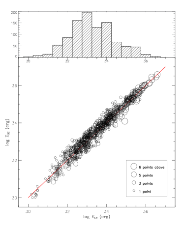
Figure 3 gives an overview of the energy distribution and shows the energy relation between LC flares and SC flares. As shown in the bottom panel, the energies are overestimated by the LC data when the energy of the flare is low. The high energy band (above $10^{36}$ erg) have a low dispersion. Presumably this is because energies are proportional to durations, and the dispersions of durations decline as the durations increase.

The profile of a flare will apparently affect the estimation of flare parameters, while LC data are hard to capture the profiles. Three parameters, the energy, the amplitude and the duration are often used to quantify flare properties in the previous work (Walkowicz et al., 2011; Maehara et al., 2012; Balona, 2013; Shibayama et al., 2013; Candelaresi et al., 2014; Ramsay & Doyle, 2014; Kitze et al., 2014; Lurie et al., 2015; Gao et al., 2016; Davenport, 2016; Gizis et al., 2017; Makarov & Goldin, 2017; Yang et al., 2017). However, LC data are used to study flare in those work. It is thus necessary to study how using LC instead of SC will affect the above three parameters.

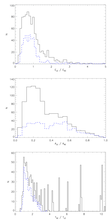
Figure 4 shows the distribution of ratios of energies, amplitudes, and durations between LC and SC flares. The solid lines are the distribution of all flares, while the blue lines represent flares with multiple points in LC data. As shown in the top panel of Figure 4, most ratios are below 1. Their peak is near 0.8, and the concentration of the distribution is obvious, which suggests LC data underestimate flare energies.

The middle panel of Figure 4 implies that one-point flares in LC data have much larger deviations from true amplitudes. Flares with multiple points underestimate amplitudes by 40% to 80%, and their distribution is wide.

The bottom panel of Figure 4 shows that durations of small flares with one point are overestimated. Their real durations are much smaller than half an hour. Flares with multiple points also have overestimated durations. Their distribution is quite wide, because of huge difference of the time resolution between the two data sets. Moreover, the durations of LC flares largely depend on baselines, which could have errors in the determination of the end time of flares.

Therefore, from above panels, we suggest that energies and amplitudes have been underestimated by LC flares, while LC durations have been overestimated. For the flares with multiple points, the mean values of these ratios demonstrate the systematical deviations of LC flares compared to SC flares. They are 75%, 40% and 147% for energies, amplitudes and durations respectively, and their standard deviations are 61.8%, 21.1% and 53.5% respectively, which can represent the uncertainties. The above results imply that basic properties of flares can be captured by LC data in spite of the existence of deviations and errors.

3.3. The Limitation of LC data

Figure 7.— Relation between energy ratios and parameters of flares. In the top panels, the horizontal axis is the difference of timings between LC and SC flares, in which the left panel shows all flares, and the right panel shows flares with multiple points in LC data. In the bottom panels, the horizontal axis is the decay rate.

The deviations of basic parameters are determined by profiles of flares. The distribution shifts of Figure 4 suggest that there are differences of profiles between LC and SC data. If LC data can capture the differences, we are able to make corrections for each flare by LC parameters, which could provide references for the future work.

The main energy of a flare is from its peak. However, the time resolution of LC data is low. It is a natural thought that the sampling timing may make great impact on the flare amplitude and the energy estimation. Figure 5 illustrates some well aligned (the difference of the sampling timings of the peaks are within 10 minutes) LC and SC flares, while Figure 6 shows some misaligned (the difference of the sampling timings of the peaks are over 10 minutes) flares. Most of the peaks of LC flares are much lower than those of SC flares, which cause 0.2 deviation from 1. However, if the peak is low, and the profile of a flare is flat, the LC energy also can be larger than the SC energy. The top panels of Figure 7 show the relation between energy ratios and difference of peak timings, which imply the energy ratio do not depend on the sampling timing, or the difference of the sampling timing is too small to affect the ratio. Thus the influence of the misaligned peak is limited.

Another factor that affects the flare amplitude of LC data is the decay rate of the peak. Because the flux of each point is a mean in a cadence period, which consists of a mount of frames. The slower the decay rate is, the closer the flux is to the actual value. This conclusion can be inferred from Figure 5 and Figure 6. A flare with a long duration of the peak has a much higher amplitude than that with a short duration of the peak. Besides, if the profile is sharp, the well-aligned peak of LC data could also be a tenth of that of SC data.

Some previous work describe the decay rate with an exponential function (e.g., Pugh et al., 2016; Van Doorsselaere et al., 2017). Here, we introduce a parameter of the LC flare: the duration from the peak to the half of the peak (DPH), and define the decay rate as the ratio of the peak to DHP. The DPHs are calculated by interpolation. The peak and DPH have high signal to noise ratios and are not affected by the end time of flares. Flares with multiple peaks are excluded in the comparison.

The bottom panels of Figure 7 show the relation between the energy ratios and the decay rates. In the left panel, there is a weak relation, and the dispersion is large. However, it can be inferred that the energy estimation of LC data decreases as the peak becomes steep.

The right panel of Figure 7 shows the same as the left panel but for the flares with multiple points. It indicates a similar relation when the decay rates are small, and the dispersion is large as well. However, the ratios are likely to be unchanged when the decay rates are large enough, and the dispersion becomes relative small. This result can also be inferred from Figure 3, which shows smaller dispersion in the high energy band.

Figure 8.— Relation between the amplitude ratios and the flare parameters. In the top panels, the horizontal axis is the difference of timings between LC and SC flares, in which the left panel shows all flares, and the right panel shows flares with at least two points in LC data. In the bottom panels, the horizontal axis is the decay rate.

The top panels of Figure 8 show relation between the amplitude ratios and the difference of peak timings. Similar to Figure 7, it implies that the influence of the misaligned peak is limited. The bottom panels of Figure 8 show relation between the amplitude ratios and the decay rates. The left panel includes all flares and shows no correlation, because one-point flares concentrate near the low band of the decay rate and have large errors.

However, as shown in the bottom right panel, there is a generally weak relation with a large dispersion. The ratios decline along with the increase of the decay rates, which demonstrates that the steeper profiles would result in larger deviations of amplitudes.

Figure 8 and Figure 7 investigate the limitation of LC data. The generally weak relations with large dispersions are presented. Obviously, LC data cannot grasp the detailed profiles of flares. It is thus hard to make correction based on LC data, whereas the limitation of LC data may reflect the tendency of the deviations to a certain extent.

4. Conclusion

The study of flare using LC data has been applied to many aspects of stellar physics. However, the basic properties derived from the LC data such as the true-flare rate, the energy, the amplitude, and the duration, systematically deviate from the results derived from the SC data.

We search flares both in LC and SC data. The search procedure and criteria are strict, and the results are checked manually. By comparing the LC data with the SC data, we have the conclusions as follows:

(1) Most flare candidates with only one point in LC data are artifacts. Few of them are true flares, while they have a large deviation from the properties derived from SC data. Most candidates with multiple points in LC data are true flares. However, some candidates with symmetric profiles may not be true flares, but have other mechanisms of flux enhancement.

On the other hand, about 60% SC flares are lost by LC data on average, although the loss rate may be much different for each star.

(2) LC data have an obvious underestimation on the flare energy. Because the main energy of a flare is from its peak, the time resolution is not enough and the profile is steep. Those characters make the peak much smaller than the true value. We compare the energy ratios between LC data and SC data, and find that LC data have underestimated energies by 25% with about 60% errors.

(3) LC data also underestimate the flare amplitude by 60% with about 20% errors, which has similar reasons as the estimation of the flare energy.

(4) The durations of LC flares are overestimated. This conclusion is determined by the steep profile of the flare and the time resolution of LC data. Because a short, burst signal can enhance the average value of the surrounding flux. Moreover, their deviations are largely scattered, which depend on the fit of baselines. This is because a flare has an exponential decay, its end point is close to the quiescent flux, and decrease slowly. Slight changes of baselines could affect the determination of the end point. LC data have overestimated durations by about 50%, and the errors are about 50%.

It is undoubted that energies and amplitudes of LC data are underestimated compared with the SC data, and durations are overestimated. However, the limitation of LC data may only be the reflection of the tendency of the deviations. The further analyses demonstrate that it is hard to make corrections for each star by LC data, because LC data cannot capture the detailed profiles of flares. A complicate profile of a flare may results in a large dispersion. For example, the SC data may have multiple peaks, or multiple flares compared with the corresponding LC flare (Davenport et al., 2014; Balona, 2015; Pugh et al., 2016). The dispersion of those relations reflects the diversity of SC flares. After the comparisons and the corrections, we suggest LC data can generally capture the basic properties of flares.

Many small flares in LC data are probably artifacts. Deviations of flare properties are determined by flare profiles. Those results may affect some important conclusions made by LC data, e.g., the proportion of flare stars (Balona, 2015; Davenport, 2016; Yang et al., 2017), the FFD given by LC data (Shibayama et al., 2013; Wu et al., 2015), the nature of superflares (Kitze et al., 2014; Wichmann et al., 2014), the strength of the magnetic field of the flaring stars (Balona, 2015; Yang et al., 2017), and the study of stellar activity (Yang et al., 2017), all of which should be considered in the future work.

Appendix

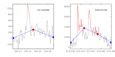
For comparison, each flare includes LC and SC data is plotted together. All images of flares are available only online. An example is shown in Figure 9. We suggest interested parties view those images to have a direct impression of this work.

Figure 9.— Light curves of two flares on KIC 1025986 and KIC 3540728. The black lines are the detrended flux in SC data, and the red lines are the flares in SC data. The blue lines are the detrended flux in LC data, and the red points are the flares in LC data. It should be noted that one LC flare may correspond to multiple SC flares as shown in the right panel, which is due to the low resolution of LC data.

References

- Balona (2012) Balona, L. A. 2012, MNRAS, 423, 3420
- Balona (2013) Balona, L. A. 2013, MNRAS, 431, 2240
- Balona (2015) Balona, L. A. 2015, MNRAS, 447, 2714
- Barstow et al. (2014) Barstow, M. A., Barstow, J. K., Casewell, S. L., Holberg, J. B., & Hubeny, I. 2014, MNRAS, 440, 1607
- Batalha et al. (2013) Batalha, N. M., Rowe, J. F., & Bryson, S. T. et al. 2013, ApJS, 204, 24
- Benz & Güdel (2010) Benz, A. O., & Güdel, M. 2010, ARA&A, 48, 241
- Borucki et al. (2010) Borucki W. J., Koch D., Basri G. et al. 2010 Sci 327 977
- Brown et al. (2011) Brown, T. M., Latham, D. W., Everett, M. E., & Esquerdo, G. A. 2011, AJ, 142, 112
- Bryson et al. (2010) Bryson S. T., Jenkins J. M., Klaus T. C. et al 2010 Proc. SPIE 7740 77401D
- Candelaresi et al. (2014) Candelaresi, S., Hillier, A., Maehara, H., Brandenburg, A., & Shibata, K. 2014, ApJ, 792, 67
- Chang et al. (2017) Chang, H.-Y., Song, Y.-H., Luo, A.-L., et al. 2017, ApJ, 834, 92
- Coughlin et al. (2016) Coughlin J. L., Mullally F., Thompson S. E. et al 2016 ApJS 224 12
- Davenport et al. (2014) Davenport, J. R. A., Hawley, S. L., Hebb, L., et al. 2014, ApJ, 797, 122
- Davenport (2016) Davenport, J. R. A. 2016, ApJ, 829, 23
- Dressing et al. (2013) Dressing, C. D. & Charbonneau, D. 2013, ApJ, 767, 95
- Gao et al. (2016) Gao, Q., Xin, Y., Liu, J.-F., Zhang, X.-B., & Gao, S. 2016, ApJS, 224, 37
- Gaulme et al. (2014) Gaulme, P., Jackiewicz, J., Appourchaux, T., & Mosser, B. 2014, ApJ, 785, 5
- Gianninas et al. (2011) Gianninas, A., Bergeron, P., & Ruiz, M. T. 2011, ApJ, 743, 138
- Gizis et al. (2017) Gizis, J. E., Paudel, R. R., Schmidt, S. J., Williams, P. K. G., & Burgasser, A. J. 2017, ApJ, 838, 22
- Hawley et al. (2014) Hawley S. L., Davenport J. R. A., Kowalski A. F. et al 2014 ApJ 797 121
- Huber et al. (2014) Huber D., Silva Aguirre V., Matthews J. M. et al 2014 ApJS 211 2
- Koch et al. (2010) Koch, D. G., Borucki, W. J., & Basri, G. et al. 2010, ApJL, 713, L79
- Kitze et al. (2014) Kitze, M., Neuhäuser, R., Hambaryan, V., & Ginski, C. 2014, MNRAS, 442, 3769
- Lurie et al. (2015) Lurie J. C., Davenport J. R. A., Hawley S. L. et al. 2015 ApJ 800 95
- Maehara et al. (2012) Maehara, H., Shibayama, T., Notsu, S., et al. 2012, Nature, 485, 478
- Makarov & Goldin (2017) Makarov, V. V., & Goldin, A. 2017, ApJ, 845, 149
- Mazeh et al. (2015) Mazeh T., Perets H. B., McQuillan A. and Goldstein E. S. 2015 ApJ 801 3
- Osten et al. (2012) Osten, R. A., Kowalski, A., Sahu, K., & Hawley, S. L. 2012, ApJ, 754, 4
- Pedersen et al. (2017) Pedersen, M. G., Antoci, V., Korhonen, H., et al. 2017, MNRAS, 466, 3060
- Pugh et al. (2016) Pugh, C. E., Armstrong, D. J., Nakariakov, V. M., & Broomhall, A.-M. 2016, MNRAS, 459, 3659
- Ramsay & Doyle (2014) Ramsay, G., & Doyle, J. G. 2014, MNRAS, 442, 2926
- Shibayama et al. (2013) Shibayama, T., Maehara, H., Notsu, S.,et al. 2013, ApJS, 209, 5
- Van Cleve & Caldwell (2009) Van Cleve, J. E. & Caldwell, D. A. 2009, Kepler Instrument Handbook, KSCI-19033
- Van Doorsselaere et al. (2017) Van Doorsselaere, T., Shariati, H., & Debosscher, J. 2017, ApJS, 232, 26
- Walkowicz et al. (2011) Walkowicz, L. M., Basri, G., & Batalha, N. et al. 2011, AJ, 141, 50
- Wichmann et al. (2014) Wichmann, R., Fuhrmeister, B., Wolter, U., & Nagel, E. 2014, A&A, 567, A36
- Wu et al. (2015) Wu, C.-J., Ip, W.-H., & Huang, L.-C. 2015, ApJ, 798, 92
- Yang et al. (2017) Yang, H., Liu, J., Gao, Q. et al. 2017, ApJ, 849, 36