An estimation of distribution algorithm for the computation of innovation estimators of diffusion processes

Abstract

Estimation of Distribution Algorithms (EDAs) and Innovation Method are recognized methods for solving global optimization problems and for the estimation of parameters in diffusion processes, respectively. Well known is also that the quality of the Innovation Estimator strongly depends on an adequate selection of the initial value for the parameters when a local optimization algorithm is used in its computation. Alternatively, in this paper, we study the feasibility of a specific EDA - a continuous version of the Univariate Marginal Distribution Algorithm (UMDAc) - for the computation of the Innovation Estimators. Numerical experiments are performed for two different models with a high level of complexity. The numerical simulations show that the considered global optimization algorithms substantially improves the effectiveness of the Innovation Estimators for different types of diffusion processes with complex nonlinear and stochastic dynamics.

1 Introduction

Diffusion processes defined through Stochastic Differential Equations (SDEs) have became an important mathematical tool for describing the dynamics of several phenomena, e.g., the dynamics of assets prices in the market, the fire of neurons, etc. In many applications, the statistical inference of diffusion processes is of great importance for model building and model selection. This inference problem consists in the estimation of the unknown parameters and unobserved components of the diffusion process given a set of discrete and noisy observations of some of its components. In this context, a variety of inference methods (see, e.g., Jim06a ) have been considered and, among them, the Innovation Estimators have been shown very useful in applications (see, e.g., Vald99 ; Oza2000 ; Riera07 ).

The computation of the Innovation Estimators involves the minimization of an objective or fitness function, which is a non-quadratic function of the parameters in most of situations. This optimization process is usually carried out by means of local optimization algorithms Vald99 ; Oza2000 ; Riera07 . In general, innovation estimators computed in that way strongly depend on the quality of the parameter’s initial value used by the local optimization algorithm. Therefore, great expertise of the users is needed to reach satisfactory estimates.

To overcome such type of difficulty, instead of a local optimization algorithm, global optimization methods as the Estimation of Distribution Algorithms (EDAs) Larranaga_et_al:2012 ; Larr2002 ; Lozano_et_al:2005 ; Muhl1996 are usually considered. In particular, EDAs comprise a group of stochastic optimization heuristics which base the search of an optimal solution on a population of individuals. In the population, each one of the individuals represents a solution to the considered optimization problem. Individuals are evaluated and a subset of them is selected according to the quality of their objective function values. EDAs use probabilistic models of the solutions to extract relevant information about the set of selected solutions. The probabilistic model is used to sample new individuals. In this way, the algorithm evolves in successive generations towards the more promising regions of the search space until a stopping criterion is satisfied. A pseudocode of a general EDA will be later presented.

EDAs can be classified according to the type of solution representation and to the way that the learning of the probability model is accomplished. The representations are discrete or continuous. Moreover, regarding the way of learning, EDAs can be classified in two classes. One class groups the algorithms that make a parametric learning of the probabilities, and the other one comprises those algorithms where structural as well as parametric learning of the model is done.

In this paper, for the computation of the Innovation Estimators of the unknown parameters of diffusion processes, we focus on a class of EDAs with continuous representation and parametric learning. As probabilistic model, we use the univariate marginals estimated from the selected population, which defines the so called Univariate Marginal Distribution Algorithm in continuous domain (UMDAc) Muhl98 . This global optimization strategy is also combined with a local optimization algorithm and tested in numerical simulations.

The paper is organized as follows. In Section 2, the estimation problem is clearly defined, and the essentials on the Innovation Method and EDAs are briefly presented. Section 4 focused on the application of the UMDAc to the parameter estimation of SDEs and the resulting algorithms are summarized. The performance of the proposed algorithms is illustrated in Section 5 in the estimation of two types of diffusion processes with complex nonlinear and stochastic dynamics. Finally, in Section 6, we present the conclusions of the paper and discuss some possible lines of future work.

2 Notations and Preliminaries

Let the continuous-discrete state space model be defined by the continuous state equation

$$dx(t)=f(t,x(t);\alpha)dt+\sum\limits_{i=1}^{m}g_{i}(t,x(t);\alpha)dw^{i}(t),\text{ for }t\geq t_{0}\in\Re.$$ (1)

and the discrete observation equation

$$z_{t_{k}}=h_{0}(t_{k},x(t_{k}))+e_{t_{k}},\ \text{ for }k=0,1,..,N\in\mathbb{N},$$ (2)

where $x(t)\in\Re^{d}$ is the state vector at the instant of time $t$, $z_{t_{k}}\in\Re^{r}$ is the observation vector at the instant of time $t_{k}$, $\alpha$ is a set of $p$ parameters, $w$ is an m-dimensional standard Wiener process, $\{e_{t_{k}}:e_{t_{k}}\thicksim\mathcal{N}(0,\Sigma)\}$, $k=\{0,..,N\}$, is a sequence of i.i.d. random vectors independent of $w$, $f,\ g_{i}:\ \Re\times\Re^{d}\rightarrow\Re^{d}$ are vector functions and $h_{0}:\ \Re\times\Re^{d}\rightarrow\Re^{r}$ is also a vector function. Here, the time discretization $\left(t\right)_{N}=\left\{t_{k}:k=0,1,\cdots,N\right\}$ is assumed to be increasing, i.e., $t_{k-1}<t_{k}$ for all $k=1,..,N$.

Let $x_{t/t_{k}}=\mathbf{E}(x(t)/Z_{t_{k}};\alpha)$ and $P_{t/t_{k}}=\mathbf{E}((x(t)-x_{t/t_{k}})(x(t)-x_{t/t_{k}})^{\intercal}/Z_{t_{k}};\alpha)$ for all $t\geq t_{k}$, where $\mathbf{E}(./.)$ denotes conditional expectation and $Z_{t_{k}}=\{z_{t_{j}}:$ $t_{j}\leq t_{k}$ and $t_{j}\in\left(t\right)_{N}\}$ is a sequence of observations. In the case that $t>t_{k}$, $x_{t/t_{k}}$ and $P_{t/t_{k}}$ are called prediction and prediction variance, respectively. If $t=t_{k}$, $x_{t_{k}/t_{k}}$ and $P_{t_{k}/t_{k}}$ are called filter and filter variance. Let $\vartheta=\{x_{t_{0}/t_{0}},P_{t_{0}/t_{0}},\alpha\}$.

The inference problem here consists in the estimation of $\vartheta$, $x_{t_{k}/t_{k}}$ and $P_{t_{k}/t_{k}}$ given the time series $Z_{t_{N}}$ with $N$ observations $z_{t_{k}}$. Usually, the inference problem for differential equations is carried out in two steps: 1) the estimation of the unknown parameters $\alpha$, and 2) the estimation of the unobserved component $x$ at each $t_{k}$, i.e., all the $x_{t_{k}/t_{k}}$ and $P_{t_{k}/t_{k}}$. In a model like (1)-(2) with $\alpha$ given, the problem of estimating the state $x(t_{k})$ from the observations $z_{t_{k}}$ is known as the nonlinear continuous-discrete filtering problem. In practical applications, $\alpha$ is commonly unknown. For this reason, the estimation of these parameters plays a central role.

3 Innovation Estimators

The Innovation Estimator $\widehat{\alpha}$ of the parameter $\alpha$ in the model (1)-(2) is defined as Jim06b :

$$\widehat{\alpha}=\arg{\underset{\alpha}{\min}\left\{q(\alpha)\right\}},$$ (3)

where

$$q(\alpha)=\left\{N\ln(2\pi)\mathbf{+}\sum\limits_{k=1}^{N}\ln(\det(\Sigma_{t_{k}/t_{k-1}}^{\mathbf{\nu}}))+\nu_{t_{k}}^{\top}(\Sigma_{t_{k}/t_{k-1}}^{\mathbf{\nu}})^{-1}\nu_{t_{k}}\right\},$$

$\nu_{t_{k}}=z_{t_{k}}-\mathbf{E}(h(t_{k},x(t_{k}))/Z_{t_{k}};\alpha)$ and $\Sigma_{t_{k}/t_{k-1}}^{\mathbf{\nu}}$ are, respectively, the discrete time innovation process and its variance.

Since the exact computation of $\nu_{t_{k}}$ and $\Sigma_{t_{k}/t_{k-1}}$ is only possible for a few particular models, in general, it is necessary to use approximate formulas. The approximations $\widetilde{\nu}_{t_{k}}$ and $\widetilde{\Sigma}_{t_{k}/t_{k-1}}^{\mathbf{\nu}}$ are recursively computed with the following Local Linearization filtering algorithm Jim03 , for $k=0,..,N-1$:

1. Prediction

   $$y_{t_{k+1}/t_{k}}=y_{t_{k}/t_{k}}+\int\limits_{0}^{t_{k+1}-t_{k}}(A_{k}y_{(t_{k}+t)/t_{k}}+a_{k}(t))dt$$

   $$Q_{t_{k+1}/t_{k}} = Q_{t_{k}/t_{k}}+\int\limits_{0}^{t_{k+1}-t_{k}}\{A_{k}Q_{(t_{k}+t)/t_{k}}+Q_{(t_{k}+t)/t_{k}}A_{k}^{\intercal}$$

   $$+\ \sum\limits_{i=1}^{m}B_{i,k}(Q_{(t_{k}+t)/t_{k}}+y_{(t_{k}+t)/t_{k}}y_{(t_{k}+t)/t_{k}}^{\intercal})B_{i,k}^{\intercal}$$

   $$+\ \sum\limits_{i=1}^{m}B_{i,k}y_{(t_{k}+t)/t_{k}}b_{i,k}^{\intercal}(t)+b_{i,k}(t)y_{(t_{k}+t)/t_{k}}^{\intercal}B_{i,k}^{\intercal}$$

   $$+\ \sum\limits_{i=1}^{m}b_{i,k}(t)b_{i,k}^{\intercal}(t)\}dt,$$

2. Innovation

   $$\widetilde{\nu}_{t_{k+1}}=z_{t_{k+1}}-h_{0}(y_{t_{k+1}/t_{k}}),$$

   $$\widetilde{\Sigma}_{t_{k+1}/t_{k}}^{\nu}=C_{k}Q_{t_{k+1}/t_{k}}C^{\intercal}_{k}+\Sigma,$$

3. Filter

   $$y_{t_{k+1}/t_{k+1}}=y_{t_{k+1}/t_{k}}+K_{t_{k+1}}\widetilde{\nu}_{t_{k+1}},$$

   $$Q_{t_{k+1}/t_{k+1}}=Q_{t_{k+1}/t_{k}}-K_{t_{k+1}}C_{k}Q_{t_{k+1}/t_{k}},$$

   where $K_{t_{k+1}}=Q_{t_{k+1}/t_{k}}C_{k}^{\intercal}\left(\widetilde{\Sigma}_{t_{k+1}}^{\nu}\right)^{-1}$ is the filter gain.

In the above algorithm the remaining notations are:

$$A_{k}=J_{f}(t_{k},y_{t_{k}/t_{k}}),\qquad B_{i,k}=J_{g_{i}}(t_{k},y_{t_{k}/t_{k}}),\quad C_{k}=J_{h_{0}}(t_{k},y_{t_{k}/t_{k}})$$

$$a_{k}(t)=f(t_{k},y_{t_{k}/t_{k}})-J_{f}(t_{k},y_{t_{k}/t_{k}})y_{t_{k}/t_{k}}+\frac{\partial f(t_{k},y_{t_{k}/t_{k}})}{\partial s}(t-t_{k}),$$

and

$$b_{i,k}(t)=g_{i}(t_{k},y_{t_{k}/t_{k}})-J_{g_{i}}(t_{k},y_{t_{k}/t_{k}})y_{t_{k}/t_{k}}+\frac{\partial g_{i}(t_{k},y_{t_{k}/t_{k}})}{\partial s}(t-t_{k}),$$

where $J_{v}$ indicates the Jacobian matrix of the vector function $v$. The algorithm starts with

$$y_{t_{0}/t_{0}}=x_{t_{0}/t_{0}},\quad Q_{t_{0}/t_{0}}=P_{t_{0}/t_{0}}$$

for each given value of $\alpha$.

Finally, the estimates $y_{t_{k}/t_{k}}$ and $Q_{t_{k}/t_{k}}$ obtained from the above filtering algorithm with $\alpha=\widehat{\alpha}$ give an approximation of the mean $x_{t_{k}/t_{k}}$ and variance $P_{t_{k}/t_{k}}$ of the states $x(t_{k})$ in the model (1)-(2).

Explicit formulas for the solution of the differential equations involved in the prediction step can be found in Jim03 or in Jim15 .

The minimization of the function $q(\alpha)$ with respect to $\alpha$ is a major difficulty in the computation of the Innovation Estimators, as it can be observed from the expression (3). In this situation, the optimization process acquires great importance for estimating the parameters of the model.

Among the difficulties of this optimization problem are the non-quadratic dependence of the fitness or objective function $q(\alpha)$ with respect to the parameters $\alpha$ due to the nonlinearity of the model (1)-(2) and the presence of parameters $\alpha$ in the highly nonlinear term corresponding to the innovation variance $\Sigma^{\nu}$. An additional difficulty is the impossibility of using local optimization methods of high convergence order since calculating the gradient or the Hessian of the objective function with regard to the parameters is not possible.

3.1 Univariate Marginal Distribution Algorithm

A pseudocode of a general Estimation of Distribution Algorithm for solving optimization problems is shown in Algorithm 1.

Table 1: Pseudocode of a general Estimation of Distribution Algorithm (EDA)

Algorithm 1: EDA

1 Set $t\Leftarrow 1$. Generate $M$ points randomly from the search space (Initial population $D_{0}$). 2 do { 3 Evaluate the fitness function at the $M$ points. 4 Select a set of points $D^{Se}_{t-1}$ according to a selection method. 5 Compute a probabilistic model from $D^{Se}_{t-1}$. 6 Sample $M$ new points according to the probability distribution previously learnt. 7 $t\Leftarrow t+1$ 8 } until Termination criteria are met

In particular, the Univariate Marginal Distribution Algorithm (UMDA) Muhl98 follows Algorithm 1, but uses univariate marginals calculated from the selected population as the probabilistic model. Theoretical studies, as well as a variety of applications of UMDA have been reported in Liv11 ; Hash2011 ; Muhl1996 ; San07 . On the other hand, applications of EDAs to problems with continuous representation comprise the use of UMDA based on Gaussian models Beng2002 ; Larr1999 ; Seb98 , Gaussian networks Beng2002 ; Lar2015 ; Larr1999 , Marginal Histogram in Continuous Domains Tsut2001 , mixtures of Gaussian distributions Bos2000a , and Voronoi based EDAs Oka2004 . In its general form, the UMDA for continuous domains (UMDAc) Larr1999 is not restricted to the use of Gaussian distributions, the density function which better fits the optimal solutions is statistically determined for each generation. For more details on EDAs for continuous domains Bosman_and_Grahl:2008 ; Bosman_and_Thierens:2006 ; Pelik99c can be consulted.

4 UMDAc-based Innovation Estimators for Diffusions

Let $\Omega=\Re^{p}$ be the search space, $X$ a random element of $\Omega$, and $X_{i}$ its $i$-th component. $F(X_{i};\theta_{i})$ and $F(X;\theta)$ will denote, respectively, the density function of $X_{i}$ and the joint density function of $X$ depending of the sets of parameters $\theta_{i}$ and $\theta=\left\{\theta_{1},..,\theta_{p}\right\}$.

In addition, $D_{l}$ and $D^{Se}_{l}$ will denote the population at the $l$-th generation and the selected population at the $l$-th generation from which the joint probability distribution of $X$ is learnt. $F_{l}\left(X;\widehat{\theta}^{l}\right)$ denotes the joint density function estimated in each generation $l$.

The pseudocode for learning the joint density function by the UMDAc at each generation $l$ is shown in Algorithm 2.

Table 2: Calculation of the probabilistic model by the Univariate Marginal Distribution Algorithm for continuous domains

Algorithm 2: UMDAc: probabilistic model

1 for $i:=1$ to $p$ { 2 Select via hypothesis test the density function $F_{l}\left(X_{i};\theta^{\ l}_{i}\right)$ which better fits the population $D^{Se}_{l-1}$ projected on $X_{i}$ 3 Obtain the maximum likelihood estimators $\widehat{\theta}^{\ l}_{i}$ for $\theta^{l}_{i}$ } The learnt joint density function is expressed as $F_{l}\left(X;\theta^{l}\right)=\prod^{p}_{i=1}F_{l}\left(X_{i};\widehat{\theta}^{\ l}_{i}\right)$

We will use the UMDAc with Gaussian distributions. By considering independence among the components of $X$ we assume that the joint density function $F(X)$ is normal $p$-dimensional and could be factorized as the product of the normal univariate marginal densities of each component $X_{i}$. Univariate marginal densities for each $X_{i}$ will be calculated as

$$F(X_{i})=\frac{1}{\sqrt{2\pi}\sigma_{i}}e^{-\frac{(X_{i}-\mu_{i})^{2}}{2\sigma_{i}^{2}}}.$$ (4)

In our optimization problem each component $X_{i}$ belongs to a bounded interval $[a_{i},b_{i}]$. A first population $D_{0}$ of $M$ points is generated according a uniform distribution. In every generation $l\ (l>1)$ with $M$ points $X^{j}$, for every component $X_{i}$ we performed the estimation of the mean $\mu_{i}$ and the standard deviation $\sigma_{i}$ by their sampling estimates,

$$\hat{\mu_{i}}=\frac{1}{M}\sum^{M}_{j=1}X^{j}_{i},~{}~{}~{}\text{ and }~{}~{}~{}\hat{\sigma_{i}}=\sqrt{\frac{1}{M}\sum^{M}_{j=1}\left(X^{j}_{i}-\hat{\mu_{i}}\right)^{2}}.$$

By considering elitism, the $\varepsilon$ points $X$ with the best solutions (minimum values of $q(\alpha)$) of the previous generation are kept in the new population. New $(M-\varepsilon)$ points $X$ are randomly generated from the normal distribution with the estimated parameters but retaining the i-th component inside the interval $[a_{i},b_{i}]$. The new $X$ are added into the original population replacing the non-selected ones. The process is repeated until a stop condition is met. Different stopping condition can be considered, as a fixed number of generations or non-improvement criterion after a given number of generations, for example. We considered a fixed number of generations, justified by some preliminary experiments and cost-benefit analysis.

In addition, we consider the strategy of combining the global and local optimization techniques in which the estimated values of the parameters obtained by EDA are used as initial values of the local technique. The application of EDAs together with local optimization techniques has been reported to notably improve the quality of the solutions for problems from different domains Muehlenbein_and_Mahnig:2002 ; Pelikan:2005 ; Zhang_et_al:2003 .

For comparison purposes, we used the MATLAB function fmincon as a Local Optimization Algorithm (LOA). This function searches for the minimum of a nonlinear multivariate function with constraints, and needs an initial estimate for this task.

In what follows we summarize with a pseudocode the three estimation algorithms considered in the paper for computing the innovation estimator (3) of the parameters $\alpha$ in the model (1)-(2).

Table 3: Algorithm for global optimization

Algorithm 3: UMDAc - Innovation estimator

1 Set $t\Leftarrow 1$. Generate $M$ points $X$ using a uniform distribution (Initial population $D_{0}$ for $\alpha$). 2 do { 3 Evaluate the fitness function $q(\alpha)$ at the $M$ points $X$. 4 Select a set of points $D^{Se}_{t-1}$ according to a selection method. 5 Compute a probabilistic model from $D^{Se}_{t-1}$ applying Algorithm 2 with $F(X)$ in Eq. (4). 6 Consider elitism: keeping the $\varepsilon$ points $X$ with the best solutions in the new population. 7 Sample $M-\varepsilon$ new points $X$ according to the probability distribution previously learnt. 8 $t\Leftarrow t+1$ 9 } until Termination criteria are met 10 $\hat{\alpha}$ is the $X$ with the minimum value of $q(\alpha)$ in the last generation.

Table 4: Global optimization with Local optimization refinement

Algorithm 4: Refined UMDAc - Innovation estimator

1 Use Algorithm 3 to find an estimate $\tilde{\alpha}$ of $\alpha$. 2 Set $\alpha_{0}\Leftarrow\tilde{\alpha}$. 3 Compute a new estimation $\hat{\alpha}$ of $\alpha$ with the MATLAB function fmincon starting at $\alpha_{0}$.

Table 5: Local optimization strategy (LOA)

Algorithm 5: LOA - Innovation estimator

1 Define $\alpha_{0}$ (Initial value for $\alpha$). 2 Compute an estimation $\hat{\alpha}$ of $\alpha$ with the MATLAB function fmincon starting at $\alpha_{0}$.

5 Numerical Experiments and Results

The objective of our experiments is to determine whether the use of UMDAc can improve the computation of Innovation Estimators for unknown parameters of discrete observed diffusion processes. To do so, we compare the Algorithms 3, 4 and 5 described above in the search of the solution to the optimization problem described by Eq. (3).

With these three algorithms, we carried out $100$ estimations of the parameters $\alpha$ for a given time series $Z_{t_{N}}$ of $N$ observations $z_{t_{k}}$ of two different types of diffusion processes. In each estimation, the initial population for Algorithms 3 and 4, and the initial value for the Algorithm 5 were randomly selected from a predefined set of possible values for each parameter. The population size $M$ for the UMDAc was decided in agreement with the approach suggested in Muhl01 , i.e., $M$ was set equal to $20$ times the number of parameters $p$ to be estimated. In order to have a quicker convergence to the optimum, truncation selection was used as the selection method of choice Muhl01 . An empirical rule previously used in Factorized Distribution Algorithm (FDA) Muhl99a to specify the truncation threshold $\tau$ locates it between $0.125$ and $0.4$. We fixed $\tau=0.3$ since this choice of $\tau$ has been already reported in previous EDA applications in continuous domains Cho04 . Elitism was implemented with $5\%$ of the population. A fixed number of generations was the stopping condition used although we also kept in mind a superior bound for the value of the objective function. All these mentioned values were selected after conducting a set of preliminary experiments.

For the following two examples of diffusion processes, the realization $Z_{t_{N}}$ of the model was computed by using the known order 1 strong Local Linearization scheme for SDEs (see, e.g., Jim12 ) on a time discretization finer than the observation times $t_{0}$,…,$t_{N}$ and then subsampling the approximate solution of $x$ at the time instants $t_{0}$,…,$t_{N}$.

5.1 Stiff state equation with additive noise

The modeling of stochastic behavior of neuronal populations has been of great interest for several years. The stochastic Fitzhugh-Nagumo equation has widely been used in analytical and simulation studies of neuronal models Tuck98 ; Tuck2003 . The biggest complexity to deal with this model is due to the stiffness of the nonlinear state equations (5)-(6), the components of the state variable change at very different rates. This behavior results in great difficulty for its numerical solution.

Let us consider the stochastic Fitzhugh-Nagumo model defined by the continuous nonlinear state equations

$$dx_{1} = 100(x_{1}-\frac{x_{1}^{3}}{3}-x_{2})dt$$ (5)

$$dx_{2} = \alpha_{1}+\alpha_{2}x_{1}dt+\alpha_{3}dw_{2}$$ (6)

and the discrete observation equation

$$z_{t_{k}}=x(t_{k})+e_{t_{k}}$$ (7)

where $x(t)\in\Re^{2}$, $z_{t_{k}}\in\Re^{2}$, $\alpha_{1}=1$, $\alpha_{2}=1$, $\alpha_{3}=0.1$, $x(0)=(x_{1}(0),x_{2}(0))=(-0.9323,-0.6732)$ and $\{e_{t_{k}}:e_{t_{k}}\thicksim\mathcal{N}(0,10^{-6})\}$.

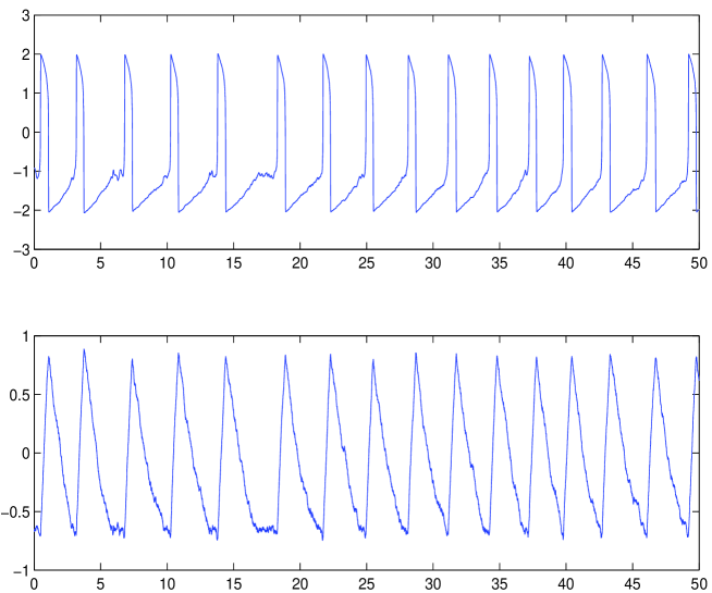
Figure 1: Realization of the solution of the state space model (5)-(6). Top:$\{x_{1}(t_{j}):j=1,\ldots,T\}.$ Bottom:$\{x_{2}(t_{j}):j=1,\ldots,T\}.$

A realization $\{x(t_{j})=(x_{1}(t_{j}),x_{2}(t_{j})):j=1,\ldots,T\}$ of the solution of the state space model (5)-(6) is shown in Figure 1 for instants of time $t_{j}=jh$, with $h=0.0005$ and $T=50$. The variations of the state variable which determines the stiff characteristics of the model are observed.

Given the state space model (5)-(7) and the single realization $\{z_{t_{k}}:k=0,\ldots,N\}$ of the equation of observations (7) with $t_{k}=k\Delta$, $\Delta=0.5$ and $N=500$, $100$ estimates of the parameter set $\alpha=(\alpha_{1},\alpha_{2},\alpha_{3})$ were carried out. Each initial estimate of $\alpha$ was uniformly generated inside of their definition intervals

$$\alpha_{1}\in[0,5],\quad\alpha_{2}\in[0,5],\quad\alpha_{3}\in[0,1].$$

Due to the complexity of this type of diffusion process, it was not possible to carry out the estimation of the set of parameters $\alpha$ using the Algorithm 5. To obtain a solution with the Matlab function fmincon of Algorithm 5 is essential to have a very good initial estimation for the parameters. Otherwise, the algorithm does not converge. For this reason, the results of the estimation with Algorithm 5 is not reported in this example.

Table 6: Parameter estimation achieved by UMDAc for the state space model (5)-(6). The interval is defined by the minimum and maximum values of the estimated parameters produced in $100$ executions of Algorithm 3.

Parameter	Real value	Estimated
$\alpha_{1}$	1	[0.9181,1.4887]
$\alpha_{2}$	1	[0.9699,1.3701]
$\alpha_{3}$	0.1	[0.1018,0.1458]

On the contrary, a satisfactory result in the estimation was obtained when the optimization is carried out via UMDAc with Algorithm 3 as it is shown in Table 6. Note that the $100$ estimations of each parameter are inside of a reduced interval, limited by the lowest and highest estimation values obtained. The histogram of the estimator for each parameter is shown at the left column of Figure 2. In the figure, dot lines correspond to the real value of the parameters, whereas dash and dot lines correspond to the mean value of the estimations.

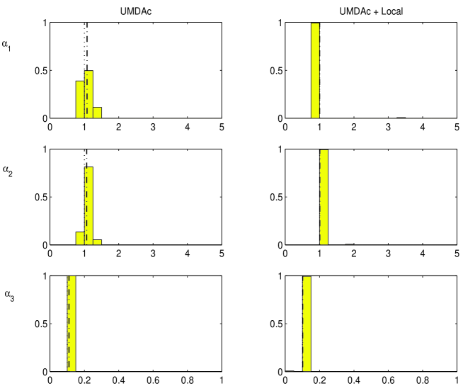
Figure 2: Histograms of the estimated values for the unknown parameters $\alpha$ in the model (5)-(6): (left) using our proposal for UMDAc, (right) combining the UMDAc and the local search algorithm.

These estimation results can be significantly improved by Algorithm 4 that use each output of Algorithm 3 as initial value of the parameters in the local optimization algorithm. Indeed, this is corroborated in the right column of Figure 2 which shows the histograms of the estimators of $\alpha$ obtained by Algorithm 4. It can be observed that the 100 estimations are all grouped very close to the true value of the parameters.

5.2 Nonlinear model with multiplicative noise

This example is of greater complexity. The state variables of the diffusion model are strongly dominated by the system noise, the signal-noise ratio is very low, and the model to be estimated is over parameterized.

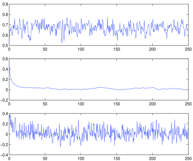
Figure 3: Realization of the solution of the state space model (8)-(9) Top: $\{x_{1}(t_{j}):j=1,\ldots,T\}$, Center: $\{x_{2}(t_{j}):j=1,\ldots,T\}$, Bottom: $\{z_{t_{k}}:k=0,\ldots,N\}$

Let us consider the following nonlinear state-space model with multiplicative noise

$$dx_{1} = (\alpha_{1}+\alpha_{2}x_{1})dt+\alpha_{3}\sqrt{x_{1}}dw_{1}$$ (8)

$$dx_{2} = \alpha_{4}x_{2}^{2}dt+\alpha_{5}x_{1}^{2}dw_{2}$$ (9)

$$z_{t_{k}}=x_{2}(t_{k})-0.001x_{2}^{3}(t_{k})+(x_{2}(t_{k})-0.01x_{2}^{2}(t_{k}))\xi_{t_{k}}+e_{t_{k}},$$ (10)

where $x(t)\in\Re^{2}$, $z_{t_{k}}\in\Re$, $\alpha_{1}=1$, $\alpha_{2}=-1.5$, $\alpha_{3}=0.1$, $\alpha_{4}=-1$, $\alpha_{5}=0.01$, $x(0)=(x_{1}(0),x_{2}(0))=(0.5,0.5)$, $\{\xi_{t_{k}}:\xi_{t_{k}}\thicksim\mathcal{N}(0,0.01)\}$ and $\{e_{t_{k}}:e_{t_{k}}\thicksim\mathcal{N}(0,0.01)\}$.

In Figure 3 a realization $\{x(t_{j})=(x_{1}(t_{j}),x_{2}(t_{j})):j=1,\ldots,T\}$ of the solution of the model (8)-(9) at instants of time $t_{j}=jh$, with $h=0.005$ and $T=5\times 10^{4}$, is shown. A realization $\{z_{t_{k}}:k=0,\ldots,N\}$ of the equation of observations (10) with $t_{k}=k\Delta$, $\Delta=0.5$ and $N=500$ is also shown. It is possible to observe in this figure the strong component of noise in the signal and in the observations, which gives a high complexity to the estimation problem.

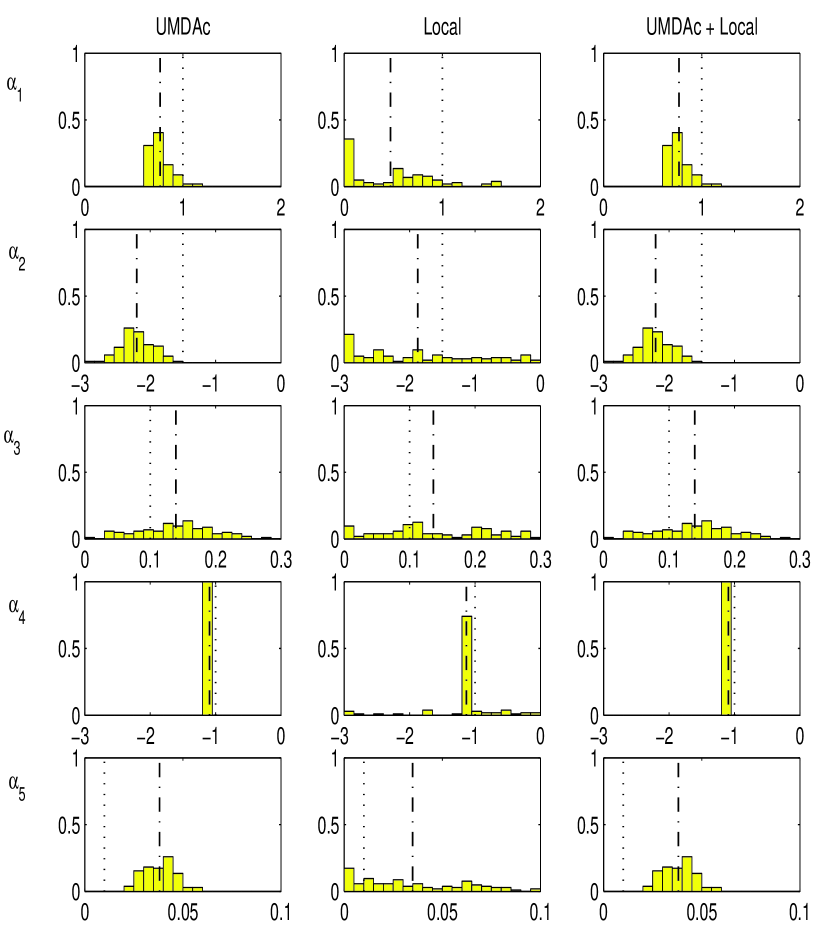
Figure 4: Histograms of the estimated values for the unknown parameters $\alpha$ in the model (8)-(10): (left) using our proposal for UMDAc, (center) using the local search algorithm, (right) combining the UMDAc and the local search algorithm.

Given the state space model (8)-(10) and a single realization of $z_{t_{k}}$, as is shown in Figure 3, $100$ estimates of the parameter set $\alpha=(\alpha_{1},\alpha_{2},\alpha_{3},\alpha_{4},\alpha_{5})$ were carried out. Each initial estimate of $\alpha$ was uniformly generated inside of their definition intervals

$$\alpha_{1}\in[0,2],\quad\alpha_{2}\in[-3,0],\quad\alpha_{3}\in[0,0.3],\quad\alpha_{4}\in[-3,0],\quad\alpha_{3}\in[0,0.1].$$

The histograms of the estimated values for $\alpha$ using the local optimization technique of Algorithm 5 are presented in the central column of Figure 4. It is possible to see that the obtained estimation is not useful when using a uniformly distributed initial value in the considered intervals for each parameter.

On the other hand, an interesting result in the estimation is obtained with the optimization Algorithms 3 and 4 via UMDAc, in the sense that all the results are located around certain biased value of the true parameters. The histograms of the estimated values of $\alpha$ with Algorithm 3 are shown in the column on the left of Figure 4, while the results obtained with Algorithm 4 are shown in the column on the right. In this case, the estimation of Algorithm 4 does not improve the results of Algorithm 3, which confirms that the local optimization algorithm is not useful for this problem.

For a better explanation of the complexity of this optimization problem, the evaluation of the fitness function around the mean values of the estimated values of the parameters is shown in Figure 5, by moving the values of only a parameter $\alpha_{i}$. In general, the fitness function is almost flat, which is even more evident for the third coordinate. The existence of a local minimum for the third parameter could be observed making a bigger rescaling in the considered interval. However, note that in this extreme situation the mean value of the estimated parameters $\alpha_{1}$, $\alpha_{2}$, $\alpha_{4}$, and $\alpha_{5}$ are quite close to the minimum value of the fitness function for each parameter, which reveals the good performance of the Algorithms 3 and 4. This demonstrates the robustness of the UMDAc in the case of having small deviations from the typical assumptions required for its use.

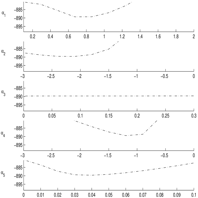
Figure 5: Evaluation of the fitness function keeping fixed all the coordinates of $\alpha$ except $\alpha_{i}$ in the model (8)-(10).

6 Conclusions

In this paper, we have considered two optimization methods based on the Estimation of Distribution Algorithms for computing the Innovation Estimators of the unknown parameters of diffusion processes given a set of discrete and noisy observations. The first method is exclusively based on a variant of the known Univariate Marginal Distribution Algorithm in continuous domain, whereas the second method includes a refinement for the outputs of the first one via a local optimization algorithm. The performance of these two optimization methods were evaluated in the parameter estimation of two types of diffusion models with complex nonlinear and stochastic dynamics. The numerical simulations demonstrate the feasibility of the considered method for the parameter estimation in situations where local optimization algorithms fail. This is particularly relevant in practice when adequate initial values for the parameters to be estimated are not available or when the diffusion model has highly nonlinear parameters to be estimated from highly noisy observations.

While our results show that UMDAc is able to deal with optimization scenarios where the commonly applied local optimization methods fail, there are still room for improvement. In particular, other EDAs that explicitly model and exploit multivariate interactions between the parameters of the fitness function are worth to be evaluated in the computation of Innovation Estimators of diffusion processes. We leave this question as a line of future research.

- (1) J. Jimenez, R. Biscay, and T. Ozaki, “Inference methods for discretely observed continuous-time stochastic volatility models: A commented overview,” Asia-Pacific Financial Markets, Vol. 12, pp. 109–141 (2006)
- (2) P. Valdes, J. C. Jimenez, J. Riera, R. Biscay, and T. Ozaki, “Nonlinear EEG analysis based on a neural mass model,” Biological cybernetics, Vol. 81, no. 5-6, pp. 415–424 (1999)
- (3) T. Ozaki, J. Jimenez, and V. Haggan-Ozaki, “The role of the likelihood function in the estimation of chaos models,” Journal of Time Series Analysis, Vol. 21, no. 4, pp. 363–387 (2000)
- (4) J. J. Riera, J. C. Jimenez, X. Wan, R. Kawashima, and T. Ozaki, “Nonlinear local electrovascular coupling. ii: From data to neuronal masses,” Human brain mapping, Vol. 28, no. 4, pp. 335–354 (2007)
- (5) P. Larrañaga, H. Karshenas, C. Bielza, and R. Santana, “A review on probabilistic graphical models in evolutionary computation,” Journal of Heuristics, Vol. 18, no. 5, pp. 795–819 (2012)
- (6) P. Larrañaga and J. A. Lozano, Eds., Estimation of Distribution Algorithms. A New Tool for Evolutionary Computation. Boston/Dordrecht/London: Kluwer Academic Publishers (2002)
- (7) J. A. Lozano, P. Larrañaga, I. Inza, and E. Bengoetxea,Eeds., Towards a New Evolutionary Computation: Advances on Estimation of Distribution Algorithms. Springer, (2006)
- (8) H. Mühlenbein and G. Paaß, “From recombination of genes to the estimation of distributions I. Binary parameters,” in Parallel Problem Solving from Nature - PPSN IV (H.-M. Voigt, W. Ebeling, I. Rechenberg, and H.-P. Schwefel, Eds.), Vol. 1141 of Lectures Notes in Computer Science, pp. 178–187, Springer, Berlin (1996)
- (9) H. Mühlenbein and T. Mahnig, “Convergence theory and applications of the factorized distribution algorithm,” Journal of Computing and Information Technology, Vol. 7, no. 1, pp. 19–32 (1998)
- (10) J. Jimenez and T. Ozaki, “An approximate innovation method for the estimation of diffusion processes from discrete data,” Journal of Time Series Analysis, vol. 27, no. 1, pp. 77–97 (2006)
- (11) J. Jimenez and T. Ozaki, “Local linearization filters for non-linear continuous-discrete state space models with multiplicative noise,” International Journal of Control, Vol. 76, no. 12, pp. 1159–1170 (2003)
- (12) J. Jimenez, “Simplified formulas for the mean and variance of linear stochastic differential equations,” Applied Mathematical Letters, Vol. 49, pp. 12–19 (2015)
- (13) L. Lozada-Chang and R. Santana, “Univariate marginal distribution algorithm dynamics for a class of parametric functions with unitation constraints,” Information Sciences, vol. 181, no. 11, pp. 2340–2355 (2011)
- (14) Hashemi. M. and Meybodi. M.R., “Univariate marginal distribution algorithm in combination with extremal optimization (eo, geo),” in Neural Information Processing – ICONIP 2011 (L. BL., Z. L., and K. J., Eds.), vol. 7063 of Lectures Notes in Computer Science, pp. 220–227, Springer, Berlin (2011)
- (15) R. Santana, P. Larrañaga, and J. A. Lozano, “Side chain placement using estimation of distribution algorithms,” Artificial Intelligence in Medicine, Vol. 39, no. 1, pp. 49–63 (2007)
- (16) E. Bengoetxea, T. Miquélez, P. Larrañaga, and J. A. Lozano, “Experimental results in function optimization with EDAs in continuous domain,” in Estimation of Distribution Algorithms, pp. 181–194, Springer (2002)
- (17) P. Larrañaga, R. Etxeberria, J. A. Lozano, and J. M. Peña, “Optimization by learning and simulation of Bayesian and Gaussian networks,” Technical Report EHU-KZAA-IK-4/99, Dept. of Computer Science and Artificial Intelligence, University of the Basque Country (1999)
- (18) M. Sebag and A. Ducoulombier, “Extending population-based incremental learning to continuous search spaces,” in Parallel Problem Solving from Nature – PPSN V, pp. 418–427, Lecture Notes in Computer Science 1498, Springer, Berlin Heidelberg (1998)
- (19) A. Ibañez, R. Armañanzas, C. Bielza, and P. Larrañaga, “Genetic algorithms and gaussian bayesian networks to uncover the predictive core set of bibliometric indices,” Journal of the American Society for Information Science and Technology, Vol. 67, p. 1703–1721 (2015)
- (20) S. Tsutsui, M. Pelikan, and D. E. Goldberg, “Evolutionary algorithm using marginal histogram in continuous domain,” in Optimization by Building and Using Probabilistic Models (OBUPM) 2001, pp. 230–233, San Francisco, California, USA (2001)
- (21) P. A. Bosman and D. Thierens, “Expanding from discrete to continuous estimation of distribution algorithms: The IDEA” in Parallel Problem Solving from Nature - PPSN VI 6th International Conference, Lecture Notes in Computer Science 1917, Springer (2000)
- (22) T. Okabe, Y. Jin, B. Sendhoff, and M. Olhofer, “Voronoi-based estimation of distribution algorithm for multi-objective optimization,” in Proceedings of the 2004 Congress on Evolutionary Computation CEC-2004, pp. 1594–1601, IEEE Press, Portland, Oregon (2004).
- (23) P. A. Bosman and J. Grahl, “Matching inductive search bias and problem structure in continuous estimation of distribution algorithms,” European Journal of Operational Research, Vol. 185, pp. 1246–1264 (2008)
- (24) P. A. Bosman and D. Thierens, “Numerical optimization with real-valued estimation-of-distribution algorithms,” in Scalable Optimization via Probabilistic Modeling: From Algorithms to Applications (M. Pelikan, K. Sastry, and E. Cantú-Paz, Eds.), Studies in Computational Intelligence, pp. 91–120, Springer-Verlag (2006)
- (25) M. Pelikan, D. E. Goldberg, and F. Lobo, “A survey of optimization by building and using probabilistic models,” Computational Optimization and Applications, Vol. 21, no. 1, pp. 5–20 (2002)
- (26) H. Mühlenbein and T. Mahnig, “Evolutionary optimization and the estimation of search distributions with applications to graph bipartitioning”, International Journal on Approximate Reasoning, Vol. 31, no. 3, pp. 157–192 (2002)
- (27) M. Pelikan, Hierarchical Bayesian Optimization Algorithm. Toward a New Generation of Evolutionary Algorithms. Studies in Fuzziness and Soft Computing, Springer (2005)
- (28) Q. Zhang, J. Sun, E. P. K. Tsang, and J. A. Ford, “Hybrid estimation of distribution algorithm for global optimization”, Engineering Computations, Vol. 21, no. 1, pp. 91–107 (2003)
- (29) H. Mühlenbein and T. Mahnig, “Evolutionary computation and beyond,” in Foundations of Real-World Intelligence (Y. Uesaka, P. Kanerva, and H. Asoh, Eds.) pp. 123–188, Stanford, California: CSLI Publications (2001)
- (30) H. Mühlenbein and T. Mahnig, “FDA – a scalable evolutionary algorithm for the optimization of additively decomposed functions,” Evolutionary Computation, vol. 7, no. 4, pp. 353–376 (1999)
- (31) D. Cho and B. Zhang, “Evolutionary continuous optimization by distribution estimation with variational bayesian independent component analyzers mixture model,” in Parallel Problem Solving from Nature (PPSN VIII), Vol. 3242, pp. 212–221, Springer (2004)
- (32) J. Jimenez and H. de la Cruz, “Convergence rate of strong local linearization schemes for stochastic differential equations with additive noise,” BIT Numerical Mathematics, Vol. 52, pp. 357–382 (2012)
- (33) H. C. Tuckwell and R. Rodriguez, “Analytical and simulation results for stochastic Fitzhugh-Nagumo neurons and neural networks,” Journal of computational neuroscience, Vol. 5, no. 1, pp. 91–113 (1998)
- (34) H. C. Tuckwell, R. Rodriguez, and F. Y. Wan, “Determination of firing times for the stochastic Fitzhugh-Nagumo neuronal model,” Neural Computation, Vol. 15, no. 1, pp. 143–159 (2003)