An Analytic Model for Eddy Current Separation

Abstract

Eddy current separation (ECS) is a process used throughout the scrap recycling industry for separating nonferrous metals from nonmetallic fluff. To date, however, the physical theory of ECS has generally been limited to empirical approximations and numerical simulations. We therefore introduce a simplified, two-dimensional model for ECS based on a cylindrical array of permanent, alternating magnets. The result is a Fourier-series expansion that describes the total magnetic field profile over all space. If the magnets are then rotated with constant angular velocity, the magnetic fields vary as a discrete series of sinusoidal harmonics, thereby inducing electrical eddy currents in nearby conductive particles. Force and torque calculations can then be used to predict the corresponding kinematic trajectories.

I Introduction

Eddy current separation (ECS) is an integral process used throughout the recycling industry for recovering nonferrous metals from solid waste (e.g., Cu, Al, Zn), and also for separating nonferrous metals from each other [1, 2, 3, 4]. The technology operates on the principle that a time-varying magnetic field tends to induce electrical currents throughout the volume of a conductive particle. These so-called eddy currents (or Foucault currents) react to the applied magnetic field by exhibiting a distinct force of deflection that alters the kinematic trajectory of the metallic particle. If the deflection force is strong enough, it can even be used to rapidly separate highly-conductive metals (e.g. aluminum, copper, brass, etc) from other nonmetallic fluff (e.g. plastic, rubber, and glass).

Despite the practical uses for eddy current technology, the basic theory of ECS is notoriously complex. Not only must one first be able to derive the magnetic field intensity ${\bf B}$ of some given magnetic configuration, but also the eddy current density ${\bf J}$ excited by that field throughout some conductive particle geometry. Both of these tasks are unique mathematical challenges unto themselves, thus making it difficult to formulate a complete analytic model for the process. To date, the most popular solution has been to formulate the magnetic field profile in terms of a Fourier series of cylindrical harmonics and then approximate the coefficients through empirical measurements. The process seems to have originated with the work of Rem, et al [5, 6], and has since been applied by numerous other publications as well [7, 8, 9]. Alternatively, one may simply calculate the magnetic field profile using finite-element analysis and then apply a similar approximation numerically [10, 11].

What is needed is a closed-form mathematical model that completely solves for the magnetic field profile around an ECS without any reliance on computationally-intense simulations or measurement-based approximations. Not only will this greatly reduce the computational time required to model the trajectories of various metal particles, but it also provides mathematical insights into the physical nature of the process itself. Only by quantifying the various factors that contribute to particle separation can we efficiently explore new ways to optimize the technology for industrial applications.

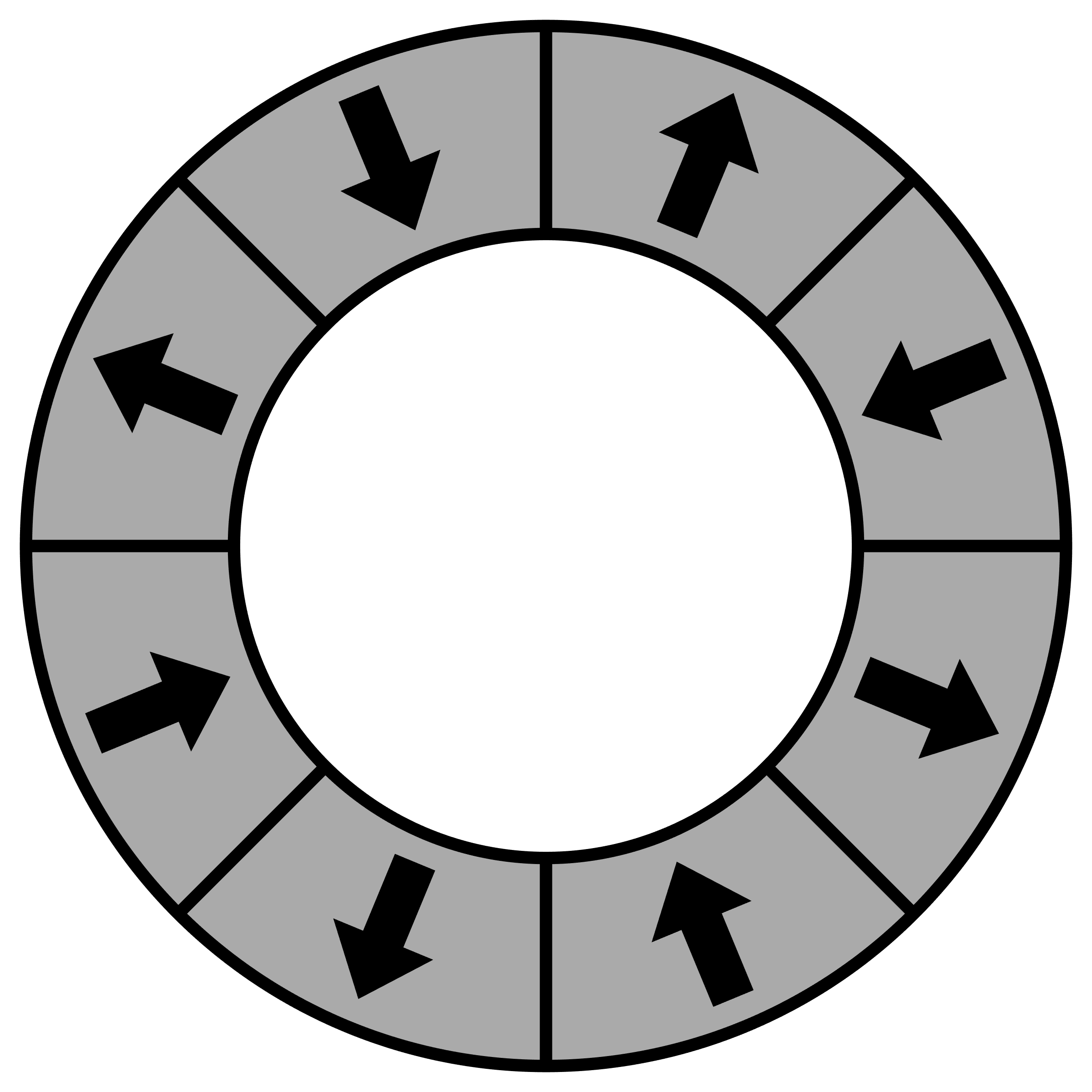
Figure 1: An eddy current separator represented as a cylindrical array of $K$ magnetized bars with alternating magnetization vector ${\bf M}$. The inner and outer radii are given as $R_{a}$ and $R_{b}$, respectively.

Figure 1 shows an idealized depiction a typical eddy current separator that will be considered in this work. An array of magnetized bars are wrapped around in a closed, hollow cylinder with inner radius $R_{a}$ and outer radius $R_{b}$. The array may be treated as having infinite extent along $z$ so that $\partial/\partial z=0$. The total number of bars is defined by an even number $K$, with $K=16$ and $K=32$ being common values for industrial separators. Each segment along the ECS is also assumed to have some permanent magnetization vector ${\bf M}$ pointing radially outward with alternating signs.

Our first goal is to solve for the magnetic field profile ${\bf B}(x,y)$ throughout all space. We will then introduce a rotational velocity ${\bm{\omega}}=\omega\hat{\bf z}$ and calculate the time-domain magnetic field profile around the bars. After that, we shall introduce a metal particle to the field and calculate the corresponding forces acting on it as it travels over the top of the ECS. This will allow us to finally track the trajectories of various metal particles as they are hurled away by the spinning magnets.

II Theoretical Background

We begin with Maxwell’s equations for linear, isotropic, nonmagnetic media in their static (zero frequency) formulation such that $d/dt=0$. In particular, the static formulation of Ampere’s law states that

$$\nabla\times{\bf B}=\mu_{0}{\bf J}~{},$$ (1)

where ${\bf B}$ is the magnetic field intensity, ${\bf J}$ is the electric current density, and $\mu_{0}$ is the permeability of free space. For the special case of a permanently magnetized material, the total current density ${\bf J}$ represents the circulating flow of charge within the very atoms of the array. The phenomenon is inherently quantum mechanical in nature and arises primarily from the unbalanced spin of electrons in certain materials [12, 13]. Since no net charges can ever build up from this flow of current, we may conclude that ${\bf J}$ has zero divergence and is thus solenoidal. We therefore express ${\bf J}$ as curl of another vector field ${\bf M}$, called the magnetization field, such that

$${\bf J}=\nabla\times{\bf M}~{}.$$ (2)

The physical interpretation of ${\bf M}$ is that of a net magnetization per unit volume. As such, the magnitude and direction of ${\bf M}$ is determined by the applied magnetic field that originally charged the magnet during fabrication.

Substitution into Ampere’s law next reveals

$$\nabla\times\left({\bf B}/\mu_{0}-{\bf M}\right)=0~{}.$$ (3)

We now introduce the auxiliary magnetic field ${\bf H}$ which is classically defined as

$${\bf H}={\bf B}/\mu_{0}-{\bf M}~{}.$$ (4)

Since ${\bf H}$ is an irrotational vector field, we may infer the existence of a scalar field $\Phi$, called the magnetic scalar potential, such that ${\bf H}=-\nabla\Phi$. Substitution back into (4) thus produces

$$\nabla\Phi={\bf M}-{\bf B}/\mu_{0}~{}.$$ (5)

If we now take the divergence of both sides, then Gauss’ law requires $\nabla\cdot{\bf B}=0$ and we are left with

$$\nabla^{2}\Phi=\nabla\cdot{\bf M}~{}.$$ (6)

We immediately recognize (6) as the well-known Poisson equation with $\nabla\cdot{\bf M}$ serving as the forcing function. As such, an analogous problem in electrostatics would be the electric scalar potential $V$ (i.e., voltage) arising from a volumetric charge density $\rho$.

Since our present problem is cylindrical in symmetry, we may recall that the Laplacian in polar coordinates is given as

$$\nabla^{2}\Phi=\frac{1}{r}\frac{\partial}{\partial r}\left(r\frac{\partial\Phi}{\partial r}\right)+\frac{1}{r^{2}}\frac{\partial\Phi}{\partial\phi^{2}}~{}.$$ (7)

where $(r,\phi)$ are the radial and angular coordinates. Using the method of separation of variables [15], the general solution to $\Phi(r,\phi)$ is known to satisfy

$$\Phi={\big{[}}Ar^{-\lambda}+Br^{\lambda}{\big{]}}\big{[}C\cos(\lambda\phi)+D\sin(\lambda\phi)\big{]}~{},$$ (8)

where $A$, $B$, $C$, and $D$ are arbitrary coefficients and $\lambda$ is the separation constant. Solutions to these constants depend on the boundary conditions over the domain of interest, which are addressed in the following sections.

III Boundary Conditions

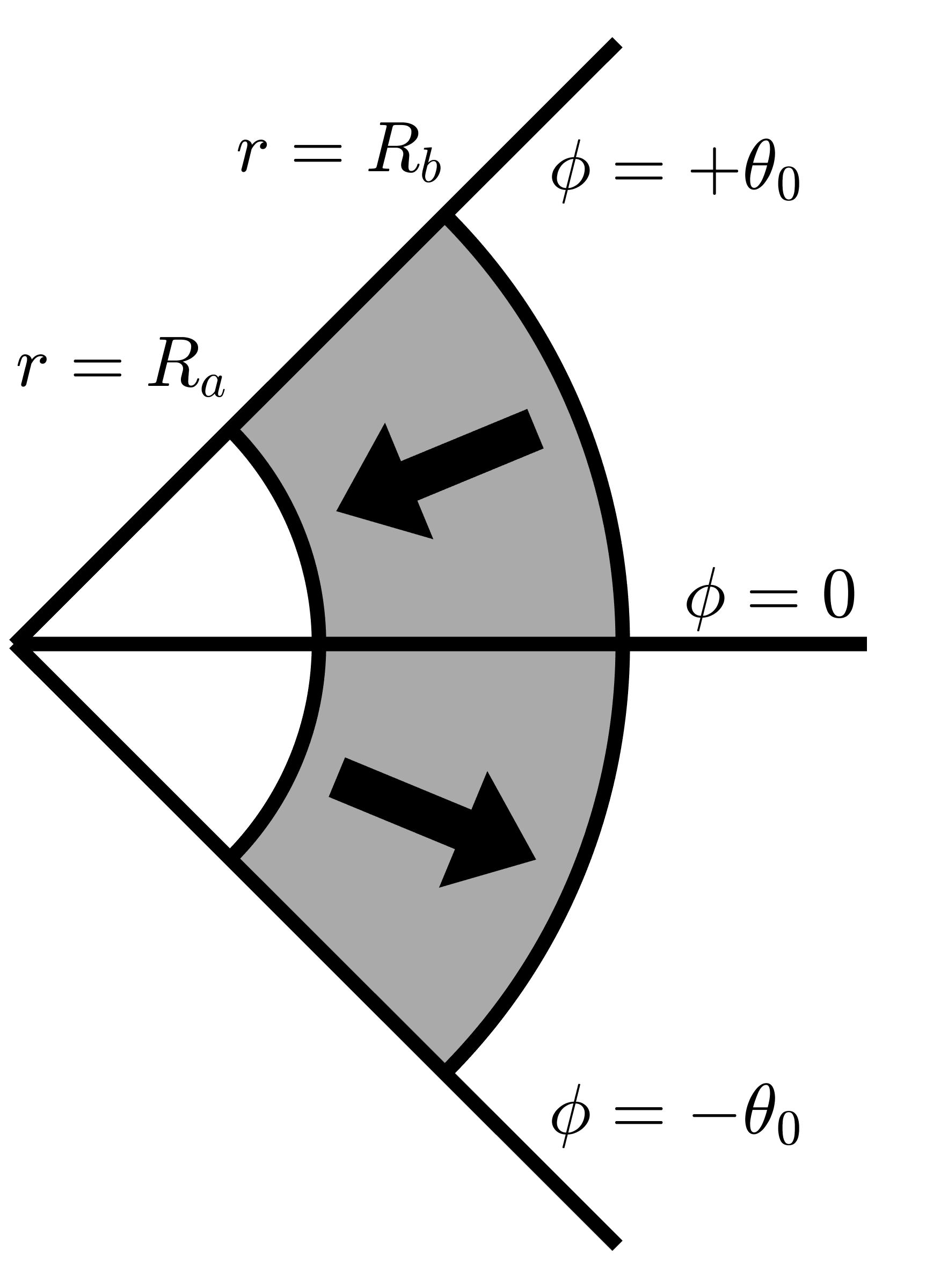
Figure 2: Unit cell of angular symmetry. The magnetic field profile repeats along arbitrary rotations of $\pm 2\theta_{0}$.

Due to the angular symmetry of the system, we may limit our focus strictly to the region depicted in Figure 2. We can then impose periodicity along arbitrary rotations of $\pm 2\theta_{0}$, where

$$\theta_{0}=2\pi/K~{}.$$ (9)

Next, we need to impose a magnetization field ${\bf M}$ along the magnetic bars. Expressing this condition in polar coordinates, the region defined by $R_{a}\leq r\leq R_{b}$ is written as

$${\bf M}(r,\phi)=\hat{\bf r}\frac{M_{a}R_{a}}{r}\begin{cases}+1&(-\theta_{0}\leq\phi<0)\\ -1&(0<\phi\leq+\theta_{0})\end{cases},$$ (10)

where $\hat{\bf r}={\bf r}/|{\bf r}|$ is the radial unit vector. Outside of $R_{a}\leq r\leq R_{b}$, we simply let ${\bf M}=0$.

The reason for formulating ${\bf M}$ in this way is to ensure that $\nabla\cdot{\bf M}$ is zero everywhere except for the discontinuities along $r=R_{a}$ and $r=R_{b}$. In practice, however, this may not be perfectly accurate since ferromagnetic materials are typically charged by applying a uniform magnetic field. Fortunately, if $R_{a}$ and $R_{b}$ are relatively large, then this distinction is not significant and the approximation should be reasonably accurate.

Using electrostatic theory as an analogy, we can imagine a mathematically equivalent system that is comprised of alternating strips of positive and negative surface charge density along $r=R_{a}$ and $r=R_{b}$. We may therefore express $\Phi$ as a linear superposition between two distinct contributions, labeled $\Phi_{a}$ and $\Phi_{b}$, representing the surface charges along the inner and outer radii. Each of these functions must then be split into two more distinct contributions representing outer and inner regions with respect to each surface. For example, we let $\Phi_{a}=\Phi_{a}^{+}+\Phi_{a}^{-}$ to denote the contributions along $r>R_{a}$ and $r<R_{a}$, respectively. Likewise, $\Phi_{b}$ has two contributions, $\Phi_{b}^{+}$ and $\Phi_{b}^{-}$, defined by the regions $r>R_{b}$ and $r<R_{b}$. The total scalar potential $\Phi$ is then expressed as a linear superposition of all four terms, written as

$$\Phi=\Phi_{a}^{+}+\Phi_{a}^{-}+\Phi_{b}^{+}+\Phi_{b}^{-}~{}.$$ (11)

As we shall find out shortly, the derivation of each potential function follows a nearly identical procedure. Thus, any solution found for one of them effectively gives us the solution for all four. We shall therefore focus our attention specifically on $\Phi_{a}^{+}$ and let the other three contributions follow naturally from basic transformations.

Beginning with our first boundary condition, we simply require that $\Phi_{a}^{+}$ remain bounded as $r\to\infty$. The immediate consequence is thus $B=0$. For our second boundary condition, we may further impose odd symmetry about the line along $\phi=0$. This likewise forces $C=0$, leaving the the more compact expression

$$\Phi_{a}^{+}=Ar^{-\lambda}\sin(\lambda\phi)\quad(r>R_{a})~{}.$$ (12)

For our third boundary condition, we apply periodicity in the form of

$$\Phi_{a}^{+}(r,+\theta_{0})=\Phi_{a}^{+}(r,-\theta_{0})~{}.$$ (13)

The immediate implication is that $\sin(\lambda\theta_{0})=0$, which can only be satisfied if

$$\lambda_{n}=\frac{n\pi}{\theta_{0}}=\frac{nK}{2}\quad(n=1,\,2,\,3,\,\dots)~{}.$$ (14)

Since any linear combination of solutions is also a solution, the general expression for $\Phi_{a}^{+}$ can now be written as

$$\Phi_{a}^{+}(r,\phi)=\sum_{n=1}^{\infty}A_{n}r^{-\lambda_{n}}\sin(\lambda_{n}\phi)\quad(r>R_{a})~{}.$$ (15)

We immediately recognize (15) as a Fourier series along $\phi$ with polynomial decay along $r$. Following a similar argument for $\Phi_{a}^{-}$, the only difference is that $\Phi_{a}^{-}\to 0$ as $r\to 0$. The general expression for $\Phi_{a}^{-}$ is thus

$$\Phi_{a}^{-}(r,\phi)=\sum_{n=1}^{\infty}A_{n}r^{+\lambda_{n}}\sin(\lambda_{n}\phi)\quad(r<R_{a})~{}.$$ (16)

If we further impose continuity on $\Phi_{a}$ along $r=R_{a}$, then we find that the Fourier coefficients $A_{n}$ must be the same for both functions.

To solve for the $A_{n}$ coefficients, we need to apply one final boundary condition along $r=R_{a}$. Unfortunately, the source expression $\nabla\cdot{\bf M}$ is somewhat challenging due to the discontinuity along this surface. A derivation for this condition is provided in Appendix I, with the end result yielding

$$\left.\frac{\partial\Phi_{a}^{+}}{\partial r}\right|_{r=R_{a}}=-\frac{M_{a}}{2}\begin{cases}+1&(-\theta_{0}<\phi<0)\\ -1&(0<\phi<+\theta_{0})\end{cases}.$$ (17)

Following standard methods of Fourier theory, we may take the derivative of (15) with respect to $r$, multiply by $\sin(\lambda_{m}x)$, and then integrate over $[-\theta_{0},\theta_{0}]$ to find

$$-\int\limits_{-\theta_{0}}^{+\theta_{0}}\sum_{n=1}^{\infty} \lambda_{n}A_{n}R_{a}^{-(\lambda_{n}+1)}\sin(\lambda_{n}\phi)\sin(\lambda_{m}\phi)\,d\phi$$

$$=-\frac{M_{a}}{2}\int\limits_{-\theta_{0}}^{0} \sin(\lambda_{m}\phi)\,d\phi+\frac{M_{a}}{2}\int\limits_{0}^{\theta_{0}}\sin(\lambda_{m}\phi)\,d\phi~{}.$$ (18)

By orthogonality, all summation terms on the left-hand side evaluate to zero except for $n=m$. After simplifying and solving for $A_{n}$, we quickly find that

$$A_{n}=-\frac{2M_{a}R_{a}^{\lambda_{n}+1}}{\lambda_{n}^{2}\theta_{0}}\quad(n=1,\,3,\,5,\,\dots)~{}.$$ (19)

The complete solution for $\Phi_{a}^{+}$ is now found to satisfy

$$\Phi_{a}^{+}(r,\phi)=\sum_{n=1}^{\infty}a_{n}\left(\frac{R_{a}}{r}\right)^{\lambda_{n}}\sin(\lambda_{n}\phi)\quad(r>R_{a})~{},$$ (20)

where $a_{n}=2M_{a}R_{a}/\lambda_{n}^{2}\theta_{0}$. Note that the ratio $R_{a}/r$ will always be less than or equal to unity, thus guaranteeing convergence over the infinite series.

To account for the region defined by $r<R_{a}$, we simply follow a similar derivation for $\Phi_{a}^{-}$. Letting $\Phi_{a}=\Phi_{a}^{+}+\Phi_{a}^{-}$, we find a compact solution satisfying

$$\Phi_{a}(r,\phi)=\sum_{n=1}^{\infty}a_{n}\sin(\lambda_{n}\phi)\left[G_{a}(r)\right]^{\lambda_{n}},$$ (21)

where the radial gate function $G_{a}(r)$ is a piecewise function defined as

$$G_{a}(r)=\begin{cases}r/R_{a}&(r\leq R_{a})\\ R_{a}/r&(r\geq R_{a})\end{cases}.$$ (22)

To account for the contribution from the surface at $r=R_{b}$, we again repeat the same basic derivation to find

$$\Phi_{b}(r,\phi)=\sum_{n=1}^{\infty}b_{n}\sin(\lambda_{n}\phi)\left[G_{b}(r)\right]^{\lambda_{n}},$$ (23)

where $b_{n}=-2M_{b}R_{b}/\lambda_{n}^{2}\theta_{0}$ and $M_{b}=M_{a}R_{a}/R_{b}$. The gate function $G_{b}$ likewise follows (22) but with $R_{b}$ used in place of $R_{a}$. To find the total magnetic scalar potential over all space, we simply let $\Phi=\Phi_{a}+\Phi_{b}$ and arrive at

$$\Phi(r,\phi)=\sum_{n=1}^{\infty}\sin(\lambda_{n}\phi)\left[a_{n}G_{a}(r)^{\lambda_{n}}+b_{n}G_{b}(r)^{\lambda_{n}}\right]~{}.$$ (24)

IV Magnetic Field Profile

With a solution for $\Phi$ now in hand, we can solve for the auxiliary magnetic field intensity by letting ${\bf H}=-\nabla\Phi$. Begin by recalling that the gradient operation in polar coordinates satisfies

$$\nabla\Phi=\frac{\partial\Phi}{\partial r}\hat{\bf r}+\frac{1}{r}\frac{\partial\Phi}{\partial\phi}\hat{\bm{\phi}}~{}.$$ (25)

Letting ${\bf H}=H_{r}\hat{\bf r}+H_{\phi}\hat{\bm{\phi}}$, we first solve for $H_{r}$ to find

$$H_{r}(r,\phi)=- \sum_{n=1}^{\infty}\left(\frac{\lambda_{n}}{r}\right)\sin(\lambda_{n}\phi)$$

$$\left[a_{n}u_{a}(r)G_{a}(r)^{\lambda_{n}}+b_{n}u_{b}(r)G_{b}(r)^{\lambda_{n}}\right]~{},$$ (26)

where $u_{a}$ and $u_{b}$ are step functions defined by

$$u_{a}(r)=\begin{cases}+1&(r<R_{a})\\ -1&(r>R_{a})\end{cases},$$ (27)

with a similar expression for $u_{b}$. Calculating $H_{\phi}$ likewise produces

$$H_{\phi}(r,\phi)=- \sum_{n=1}^{\infty}\frac{\lambda_{n}}{r}\cos(\lambda_{n}\phi)$$

$$\left[a_{n}G_{a}(r)^{\lambda_{n}}+b_{n}G_{b}(r)^{\lambda_{n}}\right].$$ (28)

To solve for magnetic field ${\bf B}$, we now add the magnetization field ${\bf M}$ to the H-field in accordance with

$${\bf B}=\mu_{0}({\bf H}+{\bf M})~{}.$$ (29)

It is worth noting that, for most practical applications, we are generally only interested in the region defined by $r\geq R_{b}$ where ${\bf M}=0$. In this case, the magnetic field simplifies to just ${\bf B}=\mu_{0}{\bf H}$. It is also frequently convenient to convert the solution to rectangular coordinates by making use of the identities

$$B_{x}(r,\phi) =\frac{xB_{r}(r,\phi)-yB_{\phi}(r,\phi)}{r}~{},~{}\text{and}$$ (30)

$$B_{y}(r,\phi) =\frac{yB_{r}(r,\phi)+xB_{\phi}(r,\phi)}{r}~{},$$ (31)

where $r=\sqrt{x^{2}+y^{2}}$.

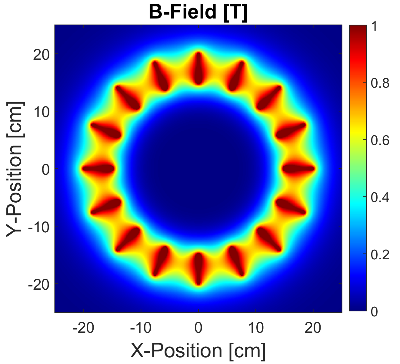
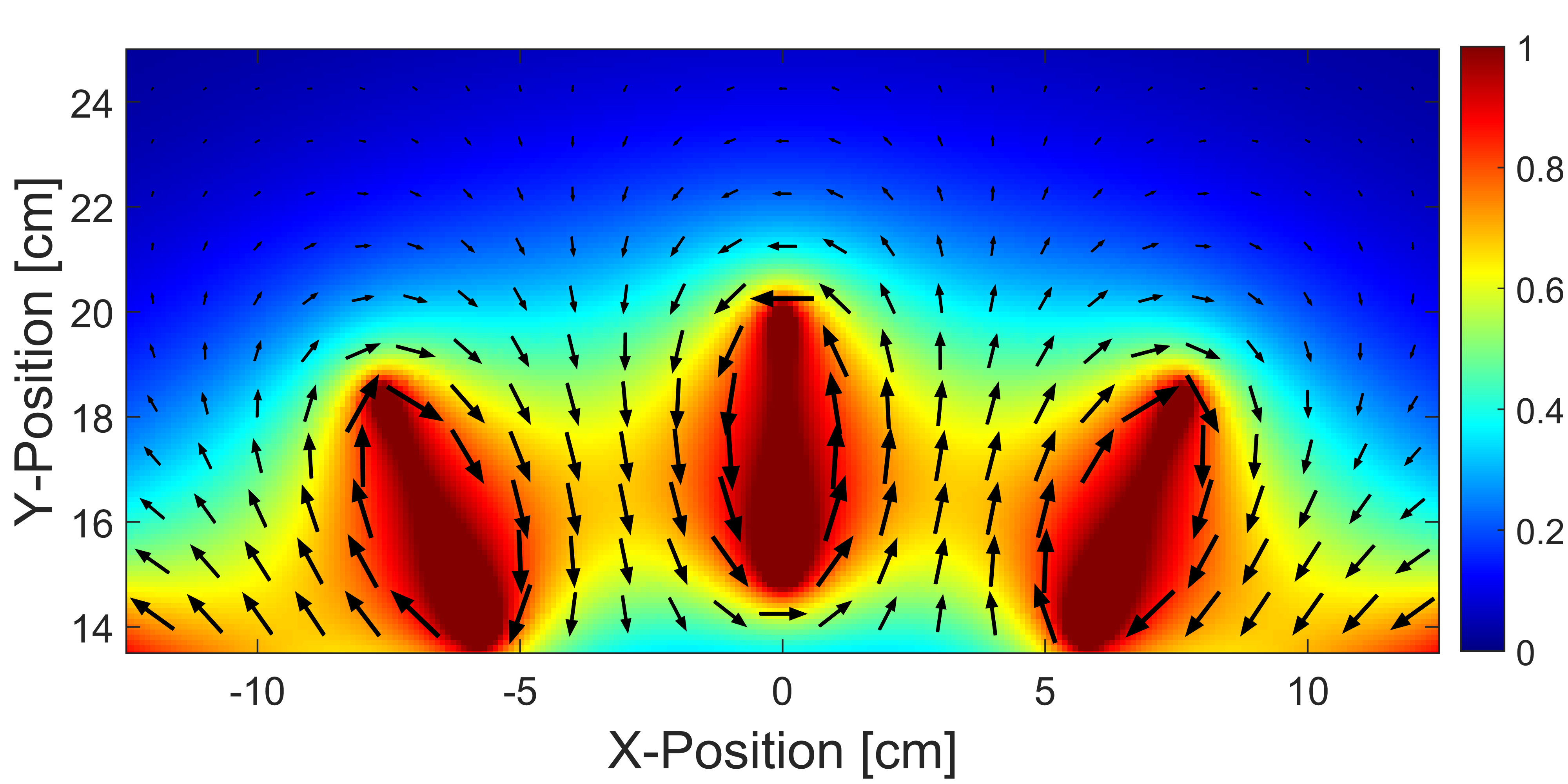
Figure 3: (Top) Magnetic field intensity for an eddy current separator with dimensions $R_{a}=15~{}$cm and $R_{b}=20~{}$cm with magnetization $M_{a}=1.0~{}$MA/m. (Bottom) Close-up profile with vectors shown.

Figure 3 shows an example calculation of the magnetic field intensity ${\bf B}$ for an eddy current separator with $K=16$ poles, inner radius $R_{a}=15~{}$cm, outer radius $R_{b}=20~{}$cm, and internal magnetization $M_{a}=1.0~{}$MA/m. Convergence of the Fourier series is surprisingly rapid, with only $N=20$ terms producing highly accurate results. The only significant truncation errors seem to appear around the boundaries at $r=R_{a}$ and $r=R_{b}$ where the magnetization vector is discontinuous.

One interesting observation is that the contribution from the inner boundary at $R_{a}$ tends to negate the contribution at $R_{b}$. The implication is that if $R_{a}\to R_{b}$, then ${\bf B}\to 0$, which should be intuitive since an array with zero thickness produces no magnetic field. We also see that if the magnetic thickness $w=R_{b}-R_{a}$ is great enough, then the contribution from $R_{a}$ becomes negligible in the outer region $r\geq R_{b}$. This can be especially useful as an approximation for the magnetic field, which greatly simplifies into

$$B_{r}(r,\phi) \approx-\sum_{n=1}^{\infty}\alpha_{n}(r)\sin(\lambda_{n}\phi)~{},\text{~{}and}$$ (32)

$$B_{\phi}(r,\phi) \approx+\sum_{n=1}^{\infty}\alpha_{n}(r)\cos(\lambda_{n}\phi)~{},$$ (33)

where the radial harmonic amplitudes satisfy

$$\alpha_{n}(r)=\frac{2\mu_{0}M_{b}}{n\pi}\left(\frac{R_{b}}{r}\right)^{\lambda_{n}+1}~{}(n=1,\,3,\,5,\,\dots)~{}.$$ (34)

Note that above formulation is perfectly consistent with the expressions provided by Rem, et al, in [6]. The key difference, however, is that the Fourier coefficients are computed exactly from the underlying geometry and thus do not require any empirical measurements to satisfy as Rem and others have traditionally done.

One practical implication for eddy current separators is the desire to maximize ${\bf B}$ in the region beyond $r>R_{b}$ while simultaneously minimizing rotational inertia. Unfortunately, these are mutually incompatible goals. Maximization of ${\bf B}$ requires the array thickness $w$ to be very large while minimum rotational inertia requires $w$ to be very small. The ideal thickness, it seems, should be just enough to reasonably satisfy (32) and (33). Any extra thickness beyond this value is essentially dead weight, as it adds nothing to the overall field intensity outside of the array.

V Velocity Transformations

To account for the relative motion between the cylindrical array and a piece of scrap metal overhead, we can imagine the magnetic field profile rotating with angular velocity ${\bm{\omega}}=\omega_{0}\hat{\bf z}$. This introduces a time dependence to the B-field written as

$${\bf B}(r,\phi,t)={\bf B}(r,\phi-\omega t)~{}.$$ (35)

Figure 4 shows a time-domain plot of the B-field components when the cylindrical array in Fig. 3 is rotated clockwise at 3000 rpm. The fields are sampled directly above the array at $(x,y)=(0,22)~{}$cm. From the perspective of a metal particle passing over the ECS, this plot represents the time-varying magnetic field profile that will induce eddy currents throughout its volume.

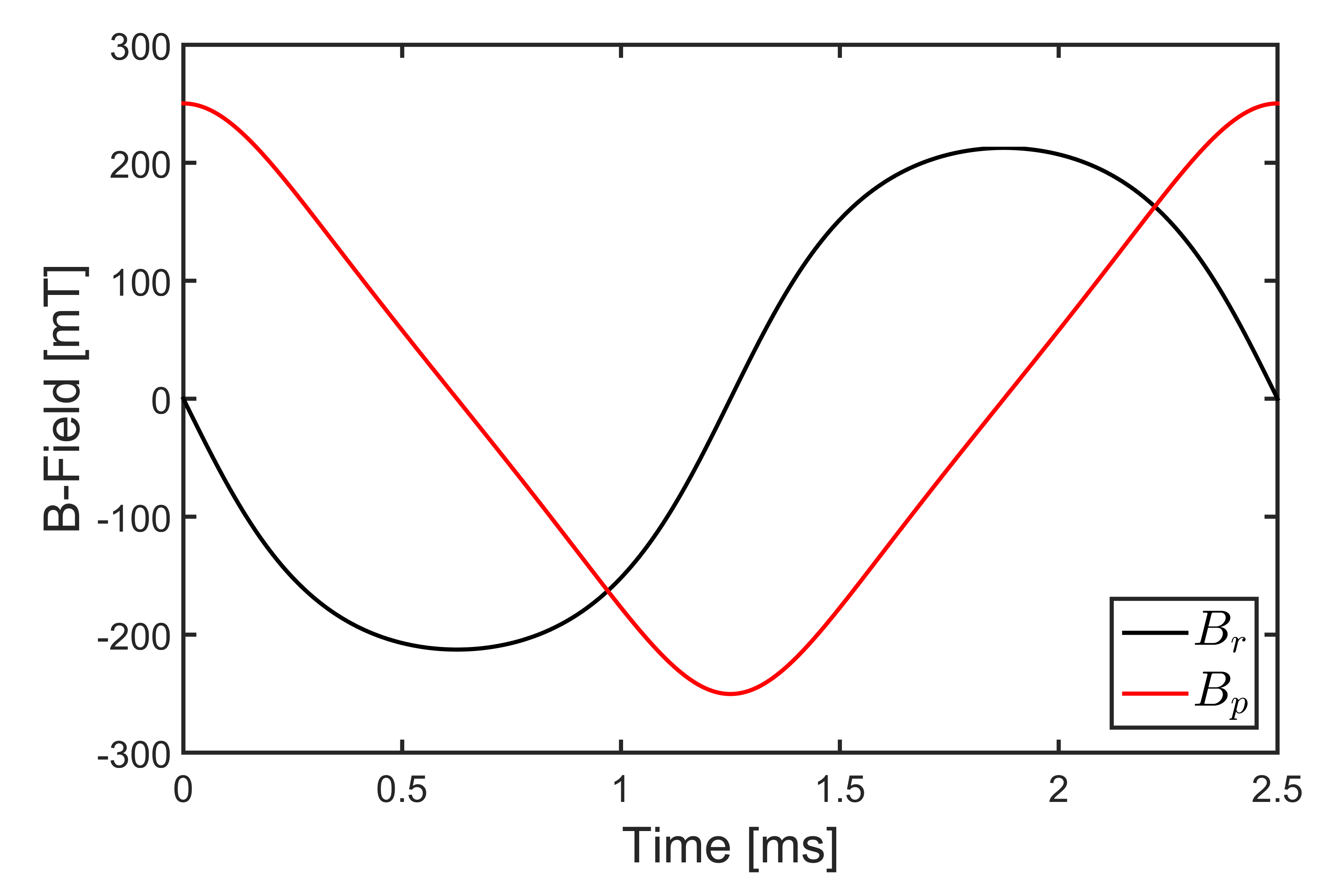
Figure 4: Time-domain signal for the magnetic field components if the magnetic array in Fig. 3 is rotated clockwise at 3000 rpm. The samples are taken at $x=0$ and $y=22~{}$cm.

The immediate implication of (35) is that the B-fields can be expressed as a Fourer series of discrete temporal harmonics. Letting $j=\sqrt{-1}$, we first write each field component as

$$B_{r}(r,\phi) =\sum_{n=1}^{\infty}\alpha_{n}(r)\,\text{Re}\left\{je^{j\lambda_{n}(\phi-\omega_{0}t)}\right\}~{},~{}\text{~{}and}$$ (36)

$$B_{\phi}(r,\phi) =\sum_{n=1}^{\infty}\alpha_{n}(r)\,\text{Re}\left\{e^{j\lambda_{n}(\phi-\omega_{0}t)}\right\}~{},$$ (37)

where Re$\{x\}$ indicates the real part of $x$. We may now express each harmonic amplitude as a complex-valued phasor with the form

$$\tilde{B}_{r}^{n}(r,\phi) =j\alpha_{n}(r)e^{j\lambda_{n}\phi}~{},~{}\text{~{}and}$$ (38)

$$\tilde{B}_{\phi}^{n}(r,\phi) =\alpha_{n}(r)e^{j\lambda_{n}\phi}~{}.$$ (39)

Note that by convention, the time-dependence of each temporal harmonic is not expressly written, but merely implied. The angular frequency of each harmonic then satisfies $\omega_{n}=\lambda_{n}\omega_{0}$. Letting $\omega_{n}=2\pi f_{n}$, we may substitute for $\lambda_{n}$ and solve for $f_{n}$ to find

$$f_{n}=\frac{n\omega_{0}}{2\theta_{0}}\quad(n=1,\,3,\,5,\,\dots)~{}.$$ (40)

Figure 5 shows the harmonic amplitudes of the time-domain signal when calculated using (34) and (40). The fundamental harmonic $(n=1)$ clearly dominates the spectrum, though some moderate energy still persists in the higher frequencies.

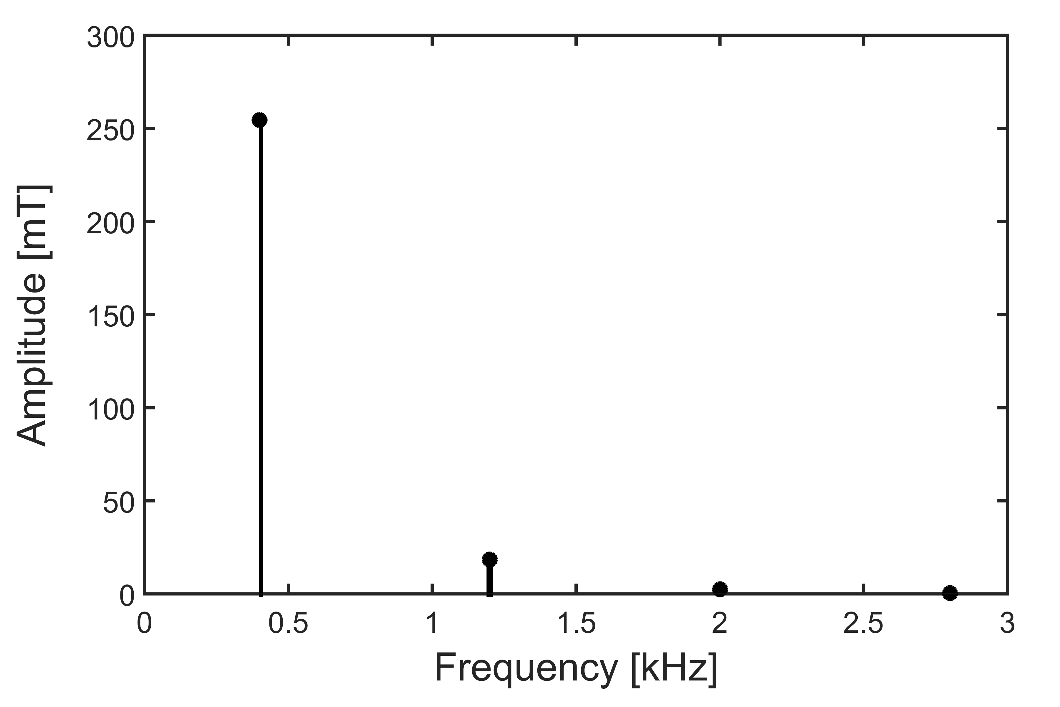
Figure 5: Approximate harmonic amplitudes for the time-domain signals depicted in Fig. 4.

VI Force Calculations

To calculate the net force acting on a metal particle, we first imagine a small conductive sphere placed inside the time-varying magnetic field expressed by (35). Due to the changing magnetic field, an electrical eddy current density $\tilde{{\bf J}}$ will be induced throughout its volume, giving rise to a magnetic moment $\tilde{\bf m}$. Following the derivation in Appendix II, a uniform, sinusoidal magnetic field $\tilde{{\bf B}}$ will give rise to a magnetic moment satisfying

$$\tilde{\bf m}=\left(\frac{6\pi a^{3}\tilde{{\bf B}}}{\mu_{0}}\right)\left(\frac{1}{k^{2}a^{2}}-\frac{\cot(ka)}{ka}-\frac{1}{3}\right)~{},$$ (41)

where $a$ is the spherical radius and $k=\sqrt{j\omega\sigma\mu_{0}}$. If we then introduce a small, linear gradient to the magnetic field $\tilde{{\bf B}}$, then the net, time-averaged force ${\bf F}_{avg}$ acting on the metal sphere can be shown to approximately satisfy [16]

$${\bf F}_{avg}=\frac{1}{2}\,\text{Re}\left\{\nabla(\tilde{\bf m}\cdot\tilde{{\bf B}}^{*})\right\}~{}.$$ (42)

For the general case of non-spherical geometries, it has also been shown that this expression can be applied with good accuracy if an equivalent spherical radius is provided [17]. We may therefore use it as a reasonable approximation for the behavior of many real-world scrap metal particles.

If the linear gradient on $\tilde{{\bf B}}$ is relatively minor, then the magnetic moment $\bf m$ may be treated as a constant value arising from the average magnetic field throughout its volume. This allows us to expand out the gradient in cylindrical coordinates such that

$$\nabla(\tilde{\bf m}\cdot\tilde{{\bf B}}^{*})=\left(\tilde{m}_{r}\frac{\partial\tilde{B}_{r}^{*}}{\partial r}+\tilde{m}_{\phi}\frac{\partial\tilde{B}_{\phi}^{*}}{\partial r}\right)\, \hat{\bf r}$$

$$+\frac{1}{r}\left(\tilde{m}_{r}\frac{\partial\tilde{B}_{r}^{*}}{\partial\phi}+\tilde{m}_{\phi}\frac{\partial\tilde{B}^{*}_{\phi}}{\partial\phi}\right)\, \hat{\bm{\phi}}~{}.$$ (43)

If we next make use of the identity

$$\frac{\partial}{\partial r}\alpha_{n}(r)=-\left(\frac{\lambda_{n}+1}{r}\right)\alpha_{n}(r)~{},$$ (44)

we can then calculate the derivatives of (38) and (39) to find

$$\frac{\partial\tilde{B}^{n}_{r}}{\partial r} =-\left(\frac{\lambda_{n}+1}{r}\right)\tilde{B}^{n}_{r}~{},$$ (45)

$$\frac{\partial\tilde{B}^{n}_{\phi}}{\partial r} =-\left(\frac{\lambda_{n}+1}{r}\right)\tilde{B}^{n}_{\phi}~{},$$ (46)

$$\frac{1}{r}\frac{\partial\tilde{B}^{n}_{r}}{\partial\phi} =\left(\frac{j\lambda_{n}}{r}\right)\tilde{B}^{n}_{r}~{},$$ (47)

$$\frac{1}{r}\frac{\partial\tilde{B}^{n}_{\phi}}{\partial\phi} =\left(\frac{j\lambda_{n}}{r}\right)\tilde{B}^{n}_{\phi}~{}.$$ (48)

Since the fundamental harmonic apparently dominates the magnetic field spectrum, it should be reasonable to calculate ${\bf F}_{avg}$ from this term alone. If greater accuracy is desired, however, then all one need do is add up the individual forces over many discrete harmonics. For even further accuracy still, one could also drop the approximations of (32) and (33). This would be especially important for thinner magnetic arrays where $R_{a}$ is relatively close to $R_{b}$.

VII Kinematic Simulations

Once we are able to calculate the net force acting on a metal particle, it is finally possible to construct a full kinematic trajectory as it passes over the ECS. Depicted in Fig. 6, we may imagine a sampling of various metal spheres with radius $a=0.5$ cm as they travel through the magnetic field along a moving conveyor belt. The space between the magnet and the belt was assumed to be 2.0 cm with the belt traveling at a constant horizontal velocity of 2.0 m/s. For simplicity, we may also neglect any frictional forces between the belt and the metal particles as well as air resistance. Thus, the only forces of significance are gravity, the normal force of contact with the belt, and the magnetic force due to the induced eddy currents.

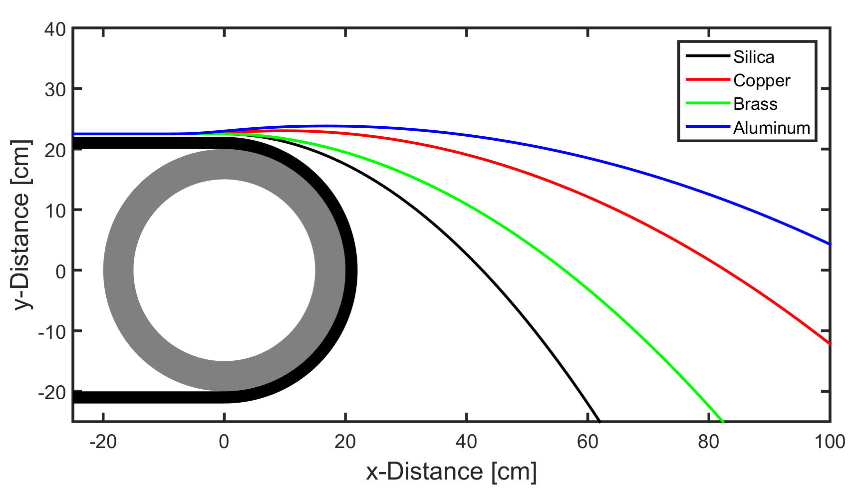
Figure 6: Kinematic trajectories for various metal spheres ($a=0.5$ cm) passing over the ECS from Fig. 3. The conveyor belt is moving with a constant horizontal velocity of 2.0 m/s while the array spins clockwise at 3000 rpm.

To simulate the kinematic trajectories of each particle, we simply calculated the force, acceleration, velocity, and position over small time increments of 0.5 ms. After each increment, a new position can be derived from the updated parameters by applying Newton’s laws of motion. For simplicity, we may neglect the contributions due to relative motion between the metal particles and the spinning array. At $\omega=3000$ rpm, the rotational velocity at the edge of the magnetic array is nearly $63$ m/s, thus dwarfing the 2.0 m/s of horizontal velocity along the conveyor.

Tab. I summarizes the four material compositions demonstrated by the model (silica, copper, brass, and aluminum). Since silica has essentially zero conductivity, its trajectory through the ECS represents the natural path taken by any free-falling body with no response to the magnetic field. The other metals have varying degrees of conductivity and density which all respond to the spinning magnetic array differently. Brass, being relatively dense with low conductivity, tends to throw very slightly in the ECS. Copper, however, has much greater conductivity and thus experiences a significantly greater deflection. Aluminum is likewise very conductive, but also much lower in density than either copper or brass. As such, we see that aluminum experiences the greatest throw distance of all.

TABLE I: Electrical conductivity and mass density for various metals under consideration.

Material	Conductivity [MS/m]	Density [g/cm3]
Silica	$\approx 0$	2.7
Copper	58.5	9.0
Brass	15.9	8.5
Aluminum	34.4	2.7

VIII Conclusions

This paper provides a set of closed-form expressions for the magnetic field profile surrounding a cylindrical array of permanent magnets like that of a typical eddy current separator. The results are congruent with the assumptions of previous publications which expressed the field profile as a Fourier series of angular harmonics in cylindrical coordinates. Rather than empirically approximate the coefficients, however, it is now possible to calculate them analytically from the physical parameters of the model.

Appendix I

The following section derives the boundary condition on $\Phi_{a}^{+}$ at $r=R_{a}$. We begin by imagining the tiny volume $V$ depicted in Fig. 7 that straddles the boundary along $r=R_{a}$ at some angle far away from $\phi=0$. If we calculate the volume integral of (6) over $V$, we find that

$$\iiint\limits_{V}\nabla^{2}\Phi\,dV=\iiint\limits_{V}\nabla\cdot{\bf M}\,dV~{}.$$ (49)

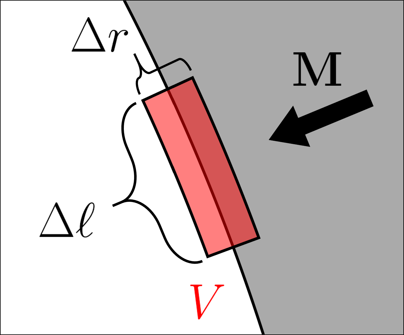
Figure 7: The volume of integration $V$ used for deriving the boundary condition on the potential function $\Phi_{a}^{+}$ at $r=R_{a}$.

By applying the divergence theorem, the volume integrals turn into surface integrals with the form

$$\oiint\limits_{S}\nabla\Phi\cdot d{\bf S}=\oiint\limits_{S}{\bf M}\cdot d{\bf S}~{},$$ (50)

where $S$ now denotes the surface enclosing $V$ and $d{\bf S}$ indicates the outward-pointing differential unit normal. Since ${\bf M}\cdot d{\bf S}$ is zero everywhere except for the outside face, the right-hand side immediately evaluates to

$$\oiint\limits_{S}{\bf M}\cdot d{\bf S}=-M_{a}\Delta\ell\begin{cases}+1&(-\theta_{0}<\phi<0)\\ -1&(0<\phi<+\theta_{0})\end{cases},$$ (51)

where $\Delta\ell\approx R_{a}\Delta\phi$.

To calculate the left-hand side of (50), we must further include the nonzero contributions from the other three faces of the surface $S$. Since $\Delta\phi$ and $\Delta r$ are very small, we can approximate this result as

$$\oiint\limits_{S}\nabla\Phi\cdot d{\bf S}\approx\Delta\ell\frac{\partial}{\partial r} \left[\Phi_{a}^{+}(R_{a},\phi)-\Phi_{a}^{-}(R_{a},\phi)\right]$$

$$+\frac{\Delta r}{R_{a}}\frac{\partial}{\partial\phi} \left[\Phi_{a}^{+}(R_{a},\phi)-\Phi_{a}^{-}(R_{a},\phi)\right].$$ (52)

By imposing continuity along $r=R_{a}$, we must conclude that $\Phi_{a}^{+}(R_{a},\phi)=\Phi_{a}^{-}(R_{a},\phi)$. If we further examine (15) and (16), we find an even symmetry about the angular derivatives and an odd symmetry about the radial derivatives such that

$$\frac{\partial}{\partial r}\Phi_{a}^{+}(R_{a},\phi) =-\frac{\partial}{\partial r}\Phi_{a}^{-}(R_{a},\phi)~{},$$ (53)

$$\frac{\partial}{\partial\phi}\Phi_{a}^{+}(R_{a},\phi) =+\frac{\partial}{\partial\phi}\Phi_{a}^{-}(R_{a},\phi)~{}.$$ (54)

Consequently, the angular derivatives sum to zero while the radial derivatives add together, giving

$$\oiint\limits_{S}\nabla\Phi\cdot d{\bf S}\approx 2\Delta\ell\frac{\partial}{\partial r}\Phi_{a}^{+}(R_{a},\phi)~{}.$$ (55)

If we now take the limit as $(\Delta r,\Delta\phi)\to 0$, the $\Delta\ell$ terms cancel and the approximations become exact. The final boundary condition thus satisfies

$$\frac{\partial}{\partial r}\Phi_{a}^{+}(R_{a},\phi)=-\frac{M_{a}}{2}\begin{cases}+1&(-\theta_{0}<\phi<0)\\ -1&(0<\phi<+\theta_{0})\end{cases}.$$ (56)

Following the same argument, it is straightforward to show that the boundary condition on $\Phi_{a}^{-}$ likewise satisfies

$$\frac{\partial}{\partial r}\Phi_{a}^{-}(R_{a},\phi)=+\frac{M_{a}}{2}\begin{cases}+1&(-\theta_{0}<\phi<0)\\ -1&(0<\phi<+\theta_{0})\end{cases},$$ (57)

with similar expressions following for $\Phi_{b}^{+}$ and $\Phi_{b}^{-}$ along $r=R_{b}$.

Appendix II

According to the derivation of [18], a metal sphere with radius $a$ and conductivity $\sigma$ will exhibit an eddy current density $\tilde{{\bf J}}$ when placed in a time-varying magnetic field $\tilde{{\bf B}}=\tilde{B}_{0}\hat{\bf z}$. Assuming an angular frequency $\omega$ of excitation, the current density evaluates to

$$\tilde{{\bf J}}(r,\theta)=\hat{\bm{\phi}}\left(\frac{-3j\omega\sigma a\tilde{B}_{0}}{2kaj_{1}^{\prime}(ka)+4j_{1}(ka)}\right)j_{1}(kr)\sin\theta~{},$$ (58)

where the function $j_{n}(x)$ is the spherical Bessel function of the first kind with order $n$ (not to be confused with the imaginary unit $j=\sqrt{-1}$). To conform with (35), however, we must adopt a phasor convention of $d/dt=-j\omega$ rather than $+j\omega$. This has the result of slightly modifying the wavenumber $k$ such that $k=\sqrt{j\omega\sigma\mu_{0}}$ rather than $k=\sqrt{-j\omega\sigma\mu_{0}}$.

Our first goal is to simplify $\tilde{{\bf J}}$. To accomplish that task, we require the following identities:

$$j_{1}^{\prime}(x) =\frac{j_{1}(x)}{x}-j_{2}(x)~{},$$ (59)

$$j_{2}(x) =\left(\frac{3}{x}\right)j_{1}(x)-j_{0}(x)~{},$$ (60)

$$j_{0}(x) =\frac{\sin(x)}{x}~{},$$ (61)

$$j_{1}(x) =\frac{\sin(x)}{x^{2}}-\frac{\cos(x)}{x}~{}.$$ (62)

This allows us to rewrite the leading coefficient on $\tilde{{\bf J}}$ such that

$$\tilde{{\bf J}}(r,\theta)=\hat{\bm{\phi}}\left(\frac{-3j\omega\sigma a\tilde{B}_{0}}{2\sin(ka)}\right)j_{1}(kr)\sin\theta$$ (63)

Our next goal is to calculate the magnetic moment $\tilde{\bf m}$, defined as

$$\tilde{\bf m} =\frac{1}{2}\int_{V}{\bf r}\times{\bf J}\,dV$$

$$=\int\limits_{0}^{2\pi}\int\limits_{0}^{\pi}\int\limits_{0}^{a}(r\hat{\bf r}\times\hat{\bm{\phi}})\tilde{J}_{\phi}(r,\theta)r^{2}\sin\theta\,drd\theta d\phi~{}.$$ (64)

The cross product $\hat{\bf r}\times\hat{\bm{\phi}}$ is a function of position and needs to be treated with care. When expressed in rectangular unit vectors, we find that

$$\hat{\bf r}\times\hat{\bm{\phi}}=-\hat{\bf x}\cos\theta\cos\phi-\hat{\bf y}\cos\theta\sin\phi+\hat{\bf z}\sin\theta~{}.$$ (65)

The integrals over $\cos\phi$ and $\sin\phi$ both evaluate to zero, leaving only the $\hat{\bf z}$ component. The integral over $\phi$ then evaluates to $2\pi$, leaving

$$\tilde{\bf m}=\hat{\bf z}\left(\frac{-6\pi j\omega\sigma a\tilde{B}_{0}}{2\sin(ka)}\right)\int\limits_{0}^{\pi}\int\limits_{0}^{a}j_{1}(kr)r^{3}\sin^{3}\theta\,drd\theta~{}.$$ (66)

The integral over $\sin^{3}\theta$ is also straightforward to solve and evaluates to $4/3$. The remaining integral requires use of (62) and evaluates to

$$\int\limits_{0}^{a}j_{1}(kr)r^{3}\,dr=\frac{(3-k^{2}a^{2})\sin(ka)-3ka\cos(ka)}{k^{2}}~{}.$$ (67)

After some simplification, the magnetic moment can then be shown to satisfy

$$\tilde{\bf m}=\left(\frac{6\pi a^{3}\tilde{{\bf B}}}{\mu_{0}}\right)\left(\frac{1}{k^{2}a^{2}}-\frac{\cot(ka)}{ka}-\frac{1}{3}\right)~{},$$ (68)

where $\tilde{{\bf B}}=\tilde{B}_{0}\hat{\bf z}$. More generally, however, we can orient $\tilde{{\bf B}}$ along any arbitrary direction and (68) would still be valid.

References

- [1] E. Schloemann, “Separation of nonmagnetic metals from solid waste by permanent magnets. I. theory,” Journal of Applied Physics, vol. 46, no. 11, pp. 5012–5021, 1975.
- [2] E. Schloemann, “Separation of nonmagnetic metals from solid waste by permanent magnets. II. experiments on circular discs,” Journal of Applied Physics, vol. 46, no. 11, pp. 5022–5029, 1975.
- [3] E. Schloemann, “Eddy-current techniques for segregating nonferrous metals from waste,” Conservation & recycling, vol. 5, no. 2–3, pp. 149–162, 1982.
- [4] J. Ruan, Q. Yiming, and Z. Xu, “Environmentally-friendly technology for recovering nonferrous metals from e-waste: Eddy current separation,” Resources, Conservation and Recycling, vol. 87, pp. 109–116, June 2014.
- [5] P. C. Rem, P. A. Leest, and A. J. van den Akker, “A model for eddy current separation,” International Journal of Mineral Processing, vol. 49, pp. 193–200, 1997.
- [6] P. C. Rem, E. M. Buender, and A. J. van den Akker, “Simulation of eddy current separators,” IEEE Transactions on Magnetics, vol. 34, no. 4, pp. 2280–2286, 1998.
- [7] M. Lungu and P. Rem, “Separation of small nonferrous particles using an inclined drum eddy-current separator with permanent magnets,” IEEE Transactions on Magnetics, vol. 38, no. 3, pp. 1534–1538, 2002.
- [8] S. Zhang, P. C. Rem, and E. Forssberg, “Particle trajectory simulation of two-drum eddy current separators,” Resources, Conservation and Recycling, vol. 26, pp. 71–90, 1999.
- [9] F. Maraspin, P. Bevilacqua, and P. Rem, “Modeling the throw of metals and nonmetals in eddy current separations,” International Journal of Mineral Processing, vol. 73, no. 1, pp. 1–11, 2004.
- [10] M. Lungu and Z. Scheltt, “Vertical drum eddy-current separator with permanent magnets,” International Journal of Mineral Processing, vol. 63, pp. 207–216, 2001.
- [11] J. Ruan and Z. Xu, “A new model of repulsive force in eddy current separation for recovering waste toner cartridges,” Journal of Hazardous Materials, vol. 192, no. 1, pp. 307–313, 2011.
- [12] J. M. D. Coey, Magnetism and Magnetic Materials. New York: Cambridge University Press, 2010.
- [13] R. C. O’Handley, Modern Magnetic Materials: Principles and Applications. Hoboken, NJ: Wiley, 2000.
- [14] J. W. Arthur, “The fudamentals of electromagnetic theory revisited,” IEEE Antennas and Propagation Magazine, vol. 50, no. 1, pp. 19–65, 2008.
- [15] D. L. Powers, Boundary Value Problems. London: Academic Press, 4 ed., 1999.
- [16] J. D. Jackson, Classical Electrodynamics. Hoboken, NJ: Wiley, 3 ed., 1999.
- [17] J. D. Ray, J. R. Nagel, D. Cohrs, and R. K. Rajamani, “Forces on particles in time-varying magnetic fields,” KONA Powder and Particle Journal, vol. (accepted for publication), 2017.
- [18] J. R. Nagel, “Induced eddy currents in simple conductive geometries,” IEEE Antennas and Propagation Magazine, vol. (accepted for publication), pp. 0–10, 2018.