The fragmentation properties of massive protocluster gas clumps: an ALMA study

Fragmentation of massive dense molecular clouds is the starting point in the formation of rich clusters and massive stars. Theory and numerical simulations indicate that the population of the fragments (number, mass, diameter, separation) resulting from the gravitational collapse of such clumps is probably regulated by the balance between the magnetic field and the other competitors of self-gravity, in particular turbulence and protostellar feedback. We have observed 11 massive, dense and young star-forming clumps with the Atacama Large Millimeter Array (ALMA) in the thermal dust continuum emission at $\sim 1$ mm with an angular resolution of $0\aas@@fstack{\prime\prime}25$ with the aim of determining their population of fragments. The targets have been selected from a sample of massive molecular clumps, with limited or absent star formation activity, and hence limited feedback. We find fragments on sub-arcsecond scales in 8 out of the 11 sources. The ALMA images indicate two different fragmentation modes: a dominant fragment surrounded by companions with much smaller mass and size, and many ($\geq 8$) fragments with a gradual change in masses and sizes. The morphologies are very different, with three sources that show filamentary-like distributions of the fragments, while the others have irregular geometry. On average, the largest number of fragments is found towards the warmer and more massive clumps. Also, the warmer clumps tend to form fragments with larger mass and size. To understand the role of the different physical parameters to regulate the final population of the fragments, we have simulated the collapse of a massive clump of $100$ and $300$ $M_{\odot}$ having different magnetic support. The 300 $M_{\odot}$ case has been run also for different initial temperatures and Mach numbers $\mathcal{M}$ to evaluate the separate role of each of these parameters. The simulations indicate that: (1) fragmentation is inhibited when the initial turbulence is low ($\mathcal{M}\sim 3$), independent of the other physical parameters. This would indicate that the number of fragments in our clumps can be explained assuming a high ($\mathcal{M}\sim 6$) initial turbulence, although an initial density profile different to that assumed can play a relevant role; (2) a filamentary distribution of the fragments is favoured in a highly magnetised clump. We conclude that the clumps that show many fragments distributed in a filamentary-like structure are likely characterised by a strong magnetic field, while the other morphologies are possible also in a weaker magnetic field.

1 Introduction

Massive and dense molecular clumps (compact structures with $M\geq 100$ $M_{\odot}$, and $n$(H₂)$\geq 10^{4}$cm^-3) in infrared-dark clouds are believed to be the birthplaces of rich clusters and high-mass O-B stars (e.g. Ragan et al. 2011; Peretto et al. 2013; Tan et al. 2013; Rathborne et al. 2015). The formation of these systems starts with the fragmentation of the parent clump occuring during its gravitational collapse, which is thus a crucial process in determining the final stellar population. In particular, the process has important implications in the theoretical debate of massive star formation ($M_{*}\geq 8$ $M_{\odot}$), because the two main competing theories assume a totally different degree of initial fragmentation: in the core-accretion models (e.g. McKee & Tan 2003), massive stars are born from the direct collapse of a near-equilibrium clump in which only one (or very few) fragments form; in the competitive accretion models (e.g. Bonnell et al. 2004), the parent clump fragments into many low-mass seeds of the order of the thermal Jeans mass which competitively accrete from the common unbound gaseous envelope.

Theoretical models and simulations predict that the number, the size, the mass, and the spatial distribution of the fragments depend strongly on which of the main competitors of gravity is dominant. The main physical mechanisms that oppose gravity during collapse are: thermal pressure, intrinsic turbulence, protostellar feedback (such as outflows or expanding H_II regions), and magnetic pressure (e.g. Krumholz 2006, Hennebelle et al. 2011, Federrath et al. 2015). However, at the beginning of the gravitational collapse, the thermal support is expected to be negligible. Mechanical feedback from nascent protostellar objects through outflows and jets, expected to be launched early in the evolution of protostars (Krumholz et al. 2014), can affect the earliest phases of the fragmentation process (Federrath et al. 2014), especially from newly born massive objects. Other feedback such as powerful stellar winds or expanding HII regions are expected to appear only in evolved stages and should not influence early fragmentation (Bate 2009). Therefore, the fragmentation at the earliest stages is influenced mainly by magnetic support, intrinsic turbulence, and protostellar feedback. However, in objects with no observational evidence of protostellar outflows, the contribution of protostar feedback to fragmentation should not dominate, and the fragment population should be mostly due to the competition between magnetic field and intrinsic turbulence. In this respect, Commerçon et al. (2011) have shown that if the magnetic support dominates the dynamical evolution, only one (or few) fragments surrounded by a non-fragmenting envelope are expected, while many small fragments with mass of the order of $\sim 0.1-1$ $M_{\odot}$ separated by projected distances of $\sim 100-1000$ au are foreseen if the magnetic support is weak.

An understanding of the formation of massive stars and rich clusters thus requires observational studies of massive dense cores in a very early stage of evolution, with both sensitivity and angular resolution appropriate to detect and resolve the smallest fragments predicted by the simulations. Surveys of massive dense clumps with adequate resolution (of the order of $\simeq 0.1-1$ ^′′, corresponding to $\sim 100-1000$ au at 1 kpc) and sensitivity (of the order of $\simeq 0.1$ $M_{\odot}$) reveal either a few fragments (e.g. Bontemps et al. 2010, Longmore et al. 2011, Palau et al. 2013, Csengeri et al. 2017), or structures with large (ten or more) number of fragments (e.g. Zhang et al. 2015, Rathborne et al. 2015, Palau et al. 2017, Henshaw et al. 2017, Cyganowski et al. 2017). In regions with many fragments, the interpretation of existing studies is very complex: in some cases, the properties of the fragments do not seem consistent with a pure gravo-turbulent scenario (e.g. Zhang et al. 2015), but in others they can be explained with a pure thermal Jeans fragmentation (Palau et al. 2015, Palau et al. 2017), or they seem to belong to complex sub-structures difficult to explain with simple theoretical models (e.g. Henshaw et al. 2017, Cyganowski et al. 2017). These results indicate that non-thermal forms of energy could play a relevant role in regulating the fragmentation at these small scales, but, overall, to date no firm conclusions can be derived.

In this work, we present an ALMA survey of 11 massive dense clumps in the thermal dust continuum emission at $\sim 278$ GHz with angular resolution $0\aas@@fstack{\prime\prime}25$, and mass sensitivity of the order of $\sim 0.1$ $M_{\odot}$, or better. In the first source belonging to this survey studied in detail, 16061–5048c1 (Fontani et al. 2016), we have detected 12 fragments, most of them located in a filament-like structure coincident with the location of an embedded 24 $\mu$m source. Although at first glance the large number of fragments could indicate a fragmentation process induced by a faint magnetic support, simulations run specifically for this object, i.e. assuming as initial conditions (temperature, mass, and Mach number) those of this source obtained from previous observations, suggest that instead its fragment population can be explained better with a strong magnetic support, especially because the filament-like morphology detected cannot be obtained with a faint magnetic support. The goal of the present work is to expand the study of 16061–5048c1 to a larger sample of objects selected similarly, in order to better understand the dominant ingredient regulating the fragmentation process in collapsing massive dense clumps in very early stages of evolution. In Sect. 2 we present the source sample and the criteria used to select it; Sect. 3 describes the observations, and Sect. 4 the observational results; in Sect. 5, we discuss our findings based on the help of numerical simulations. Finally, in Sect. 6 we give a brief summary of our work, and draw the most relevant conclusions.

2 Source sample

The targets have been selected from an initial sample of MSX-dark clumps (Beltrán et al. 2006) detected at 1.2 mm with the SIMBA bolometer at the SEST. The selection criteria applied make us confident that all objects are: (1) potential sites of massive star formation, (2) dense, (3) quiescent, (4) cold and chemically young. To satisfy these criteria, we selected clumps having the following observational properties: (1) gas mass and gas surface (and column) density consistent with being potential sites of massive star formation according to observational findings (Kauffmann & Pillai 2010); (2) detection in the high-density gas tracer N₂H⁺ (3–2) with APEX (Fontani et al. 2012), which is also the most reliable tracer of dense molecular gas (Kauffmann et al. 2017); (3) clumps isolated or having the 1.2 mm emission peak well separated ($\geq 24$^′′) from that of other clumps, and without evidence of star formation activity (Beltrán et al. 2006, Sánchez-Monge et al. 2013); (4) average CO depletion factor (ratio between expected and observed CO abundance) derived from APEX observations of C¹⁸O (3–2), $f_{\rm CO}\geq 7$ (Fontani et al. 2012), which provides evidence of the chemical youth of the clumps. Clump coordinates, distances, and main physical properties of the 11 selected clumps are summarised in Table 1.

The 1.2 mm continuum maps of all clumps are shown in Fig. 1, superimposed on the Spitzer 24 $\mu$m images. Some of the clumps are detected at 24 $\mu$m, which indicates a potential on-going star formation activity. However, the observational selection criteria (3) and (4) make us confident that possible embedded protostellar activity has not affected significantly the environment yet. Therefore, outflows, jets or other forms of mechanical protostellar feedback should not dominate in determining the fragment population.

The young evolutionary stage of the sources is also strongly supported by their low Star Formation Efficiency (SFE), given in the last Column of Table 1. The SFE has been calculated according to:

$${\rm SFE}=M_{\rm stars}/(M_{\rm gas}+M_{\rm stars})\;,$$ (1)

where $M_{\rm stars}$ is the mass already in the form of (proto-)stars calculated from the source bolometric luminosity (Giannetti et al. 2013) following the approach in Beltrán et al. (2013), and $M_{\rm gas}$ is the gas mass listed in Table 1 derived by Giannetti et al. (2013) using the dust thermal continuum emission in Beltrán et al. (2006). $M_{\rm stars}$ is computed from the bolometric luminosity assuming that the infrared emission is consistent with that of an embedded stellar cluster, although care needs to be taken due to the contribution from accretion luminosity. This caveat is especially relevant taking into account the fact that most stars should be of low mass, for which the accretion luminosity is expected to dominate. SFE is below 20$\%$ in all targets but 16061–5048c1, for which SFE is $\sim 31\%$.

Table 1: Sample of massive dense clumps and general properties: coordinates, distance, deconvolved angular diameter, gas mass, gas temperature, H₂ column density, mass surface density, CO depletion factor, and non-thermal velocity dispersion (parameters taken or derived from Beltrán et al. 2006, Giannetti et al. 2013, and Fontani et al. 2012). In the last two columns, we give the recovered flux in the ALMA images, and the Star Formation Efficiency (SFE), computed as explained in Sect. 2.

Source	R.A.;Dec.(J2000)	$l$;$b$	$d$(a)	$\theta_{\rm s}$(a)	$M_{\rm gas}$(b)	$T_{\rm k}$(b)	$N({\rm H_{2}})$(b)	$\Sigma({\rm H_{2}})$(b)	$f_{\rm CO}$(c)	$\sigma_{\rm nth}$(d)	Rec. flux(e)	SFE
	${\rm h\,m\,s}$;$\circ\,\prime\,\prime\prime$	$\circ$;$\circ$	kpc	′′	$M_{\odot}$	K	$10^{23}$ cm-2	g cm-2		km s-1	Jy/Jy	$\%$
08477–4359c1(f)	08:49:35.13;–44:11:59	264.69;–0.07	1.8	35.6	86.73	19	1.42	0.24	7	1.03	0.12/0.62	–(g)
13039–6108c6	13:07:14.80;–61:22:55	305.18;1.14	2.4	40.3	101.5	17	0.68	0.12	22	–	0	–(g)
15470–5419c1	15:51:28.24;–54:31:42	327.51;–0.83	4.1	24.2	310.2	18	1.37	0.36	35	1.02	0.01/0.56	$6\%$
15470–5419c3(f)	15:51:01.62;–54:26:46	327.51;–0.72	4.1	54.1	743.4	19	1.11	0.17	36	1.13	0.09/0.50	$3\%$
15557–5215c2(f)	15:59:36.20;–52:22:58	329.81;0.03	4.4	41.3	633.4	23	1.55	0.22	32	0.96	0.12/0.90	$4\%$
15557–5215c3	15:59:39.70;–52:25:14	329.80;0.00	4.4	35.8	194.3	15	0.49	0.09	24	–	0	$8\%$
16061–5048c1(f)	16:10:06.61;–50:50:29	332.06;0.08	3.6	28.1	284.3	25	1.66	0.31	12	1.52	0.63/1.02	$31\%$
16061–5048c4	16:10:06.61;–50:57:09	331.98;0.00	3.6	62.8	504.2	13	1.22	0.11	34	0.82	0.03/0.32	$3\%$
16435–4515c3	16:47:33.13;–45:22:51	340.31;–0.71	3.1	17.7	147	12	1.20	0.55	73	–	0	$11\%$
16482–4443c2	16:51:44.59;–44:46:50	341.24;–0.90	3.7	$\ll 24$h	59.08	16	$\gg 4.63^{h}$	0.66	9	1.40	0.07/0.23	$17\%$
16573–4214c2	17:00:33.38;–42:25:18	344.08;–0.67	2.6	7.29	108.3	17	1.89	3.4	25	1.17	0.07/0.71	$14\%$

^(a) from Beltrán et al. (2006);
^(b) from Giannetti et al. (2013);
^(c) from Fontani et al. (2012);
^(d) derived from the C¹⁸O (3–2) line width at half maximum (Fontani et al. 2012) by subtracting the thermal contribution calculated according to the gas temperature in Col. 7;
^(e) ratio between the total flux integrated inside the ALMA primary beam, and the peak flux of the SIMBA map towards the phase centre. Please note that the SIMBA main beam and ALMA primary beam are the same ($\sim 24$^′′), and that the flux ratios have been compared by correcting the SIMBA flux at 250 GHz assuming a spectral index $\beta=2$;
^(f) detected in the Spitzer 24 $\mu$m image (Fig. 1);
^(g) not possible to derive SFE because the bolometric luminosity is not available (Giannetti et al. 2013);
^(h) point-like source in the SIMBA 1.2 mm map (Beltrán et al. 2006).

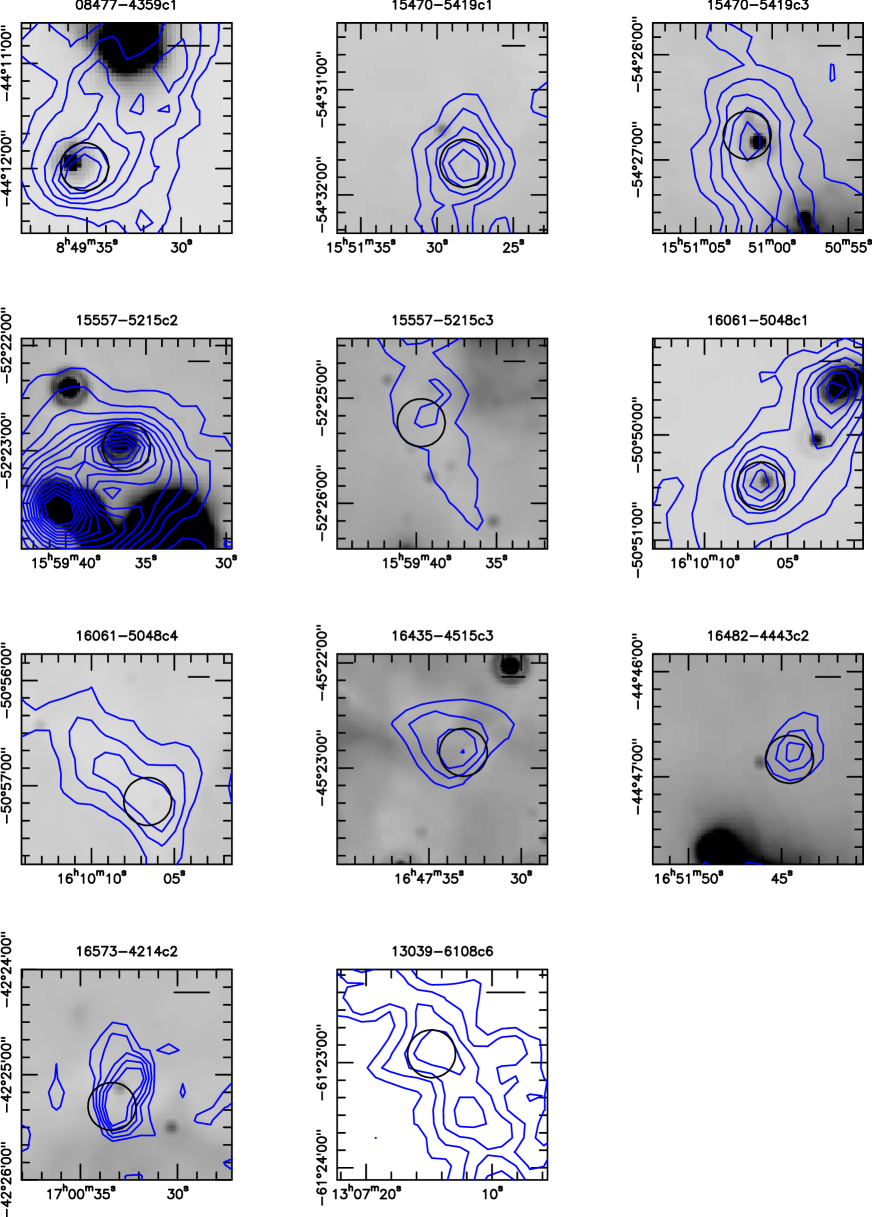
Figure 1: 1.2 mm continuum maps (contours) obtained with SIMBA at the SEST towards the 11 sources in Table 1, having an angular resolution of $\sim$24^′′. In each panel, the image on the background is the Spitzer-MIPS 24 $\mu$m map, available for all clumps but 13039–6108c6, and the circle indicates the ALMA field of view at the frequency of the N₂H⁺ (3–2) line ($\sim$22^′′) centred at the coordinates given in Table 1. The first contour and step correspond to the $3\sigma$ rms level in the map, with the exception of 16061–5048c1, in which the step is of $6\sigma$ rms (see Beltrán et al. 2006 for details). In each panel, the horizontal black bar in the top right corner shows a linear scale of 0.25 pc.

3 Observations and data reduction

Observations with the ALMA array at a frequency of $\sim 278$ GHz were performed during cycle-2 and 3 in configuration C36-6 with baselines up to 1091 m, providing an angular resolution of $0\aas@@fstack{\prime\prime}25$, and a maximum recoverable scale of $3\aas@@fstack{\prime\prime}5$. For each clump, the phase centre was set to the coordinates given in Table 1. The total integration time on each source was $\sim 18-20$ minutes. The amount of precipitable water vapour during observations was generally around $\sim 1.5-2$ mm. Bandpass and phases were calibrated by observing J1427–4206 and J1617–5848, respectively. The absolute flux scale was set through observations of Titan and Ceres. Continuum was extracted by averaging in frequency the line-free channels. The total bandwidth used is $\sim 1.7$ GHz. Calibration and imaging were performed with the CASA software (McMullin et al. 2007). Primary beam correction was always applied, and the final images were analysed following standard procedures with the software MAPPING of the GILDAS package. The angular resolution of the final images is $\sim 0\aas@@fstack{\prime\prime}25$ . We are sensitive to unresolved fragments of $\gtrsim 0.05-0.1$ $M_{\odot}$. We estimated the missing flux by comparing the total integrated flux in the primary beam of the ALMA images with the single-dish continuum measured by Beltrán et al. (2006). The ratios are given in Table 1.

4 Results

The ALMA maps of the dust thermal continuum emission, corrected for the primary beam, are shown in Fig. 2. The plot aims to compare the morphology of the fragment population in the targets to understand possible global similarities and differences. The same images, with the fragment identification and a better presentation of the emission morphology in each source, is given in Appendix A.

The dust thermal continuum emission has been decomposed into fragments according to the following criteria: (1) peak intensity greater than 5 times the noise level; (2) two partially overlapping fragments are considered as resolved if they are separate at their half peak intensity level. The minimum threshold of 5 times the noise was adopted according to the fact that some peaks at the edge of the primary beam are comparable to about 4-5 times the noise level. We decided to use these criteria and decompose the map into cores by eye instead of using decomposition algorithms (such as Clumpfind) because small changes in their input parameters could lead to big changes in the number of identified clumps (Pineda et al. 2009). In Appendix-A, from Fig. A-1 to Fig. A-7, we show the fragments identified in each source superimposed on the corresponding ALMA continuum image. We refer to Fig. 1 of Fontani et al. (2016) for the map of 16061–5048c1, with the identified fragments.

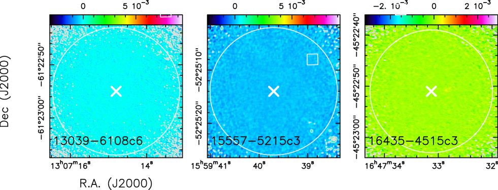
Figure 3: Same as Fig. 2 for the three objects undetected with ALMA: 13039–6108c6, 15557–5215c3, and 16435–4515c3. The location of the ATLASGAL peak is just outside the field shown in 13039–6108c6 and 16435–4515c3.

We have detected fragments in eight out of the 11 targets observed, and found at least four significant fragments in all of the eight clumps (see Figs. A-1 – A-7 in Appendix A for a detailed description). Towards 13039–6108c6, 15557–5215c3, and 16435–4515c3 we do not detect any significant (peak flux $\geq 5\sigma$ rms) fragment. The maps of these sources are shown in Fig. 3. This indicates that the emission is either more extended than the maximum recoverable angular scale ($\sim 3.5$^′′), so that we totally resolve it out, or that the phase centre is not located at the actual centre of the fragmenting region. An uncertainty in the position of the phase centre can influence both the detection and the number of fragments and the amount of missing flux. We will discuss this point further in Sect. 4.1.

4.1 Morphology of the continuum emission

The number of fragments detected ranges from a minimum of four to a maximum of 14 fragments. Fig. 2 presents all the detected sources. The morphologies are very different, with three sources in which the fragments are located along a filament-like structure, 15470–5419c3, 15557–5215c2, and 16061–5048c1, while the others have irregular geometry. About the relative intensity of the fragments within each clump, one can roughly distinguish between sources with a dominant fragment, like 15470–5419c1, 15470–5419c3, 15557–5215c2, and 16482–4443c2, and objects with a smoother distribution in intensity of the fragments. The presence of a dominant fragment can be understood from the average mass ratio between the more massive fragment and the others (Col. 6 in Table 2): for the four clumps mentioned above, this ratio is larger ($\geq 18$) than for the others ($\leq 10$). The fragment mass, $m$, has been calculated following Eq. (A1) in Fontani et al. (2016), taking the clump distances in Table 1, and assuming as dust temperature the average clump gas temperature listed in Table 1. This latter assumption is critical, because some fragments probably have higher temperatures, especially those associated with the 24 $\mu$m emission, in which the star formation activity is expected to be higher (i.e. 08477–4359c1, 15470–5419c3, 15557–5215c2, and 16061–5048c1). In these cases, our mass estimates are likely upper limits. This issue can be solved only with a high angular resolution map of the dust temperature, unavailable to date. Finally, we have assumed the same gas-to-dust ratio (100) and the same expression for the dust mass opacity index as in Fontani et al. (2016). The errors on the gas masses calculated in this way are difficult to quantify, mostly because of the large uncertainty in the mass opacity coefficient, which can be up to a factor 2-3 (e.g. Ossenkopf & Henning 1994).

Four objects have Spitzer 24 $\mu$m emission (indicated by the star in Fig. 2) within the primary beam, and in three of them, 08477–4359c1, 15557–5215c2, and 16061–5048c1, the fragments are clearly associated with the infrared source. The only exception is 15470–5419c3, for which the fragments appear totally offset from both the Spitzer source and the phase centre, at the border of the ALMA primary beam. This morphology, however, is in rough agreement with the elongated structure seen in the SIMBA map.

None of the fragments coincides with the peak of the emission as mapped by SIMBA (indicated by the crosses in Fig. 2). In general, the asymmetric location of the fragments with respect to the phase centre is in rough agreement with the asymmetric emission seen with the single-dish (see Fig. 1), but larger than the nominal pointing error (estimated to be of a few arcseconds, Beltrán et al. 2006). The exception is 16482–4443c2, in which the fragments are located to the North-East, while the SIMBA map seems rather to be slightly elongated to the West (although the SIMBA source is considered as unresolved by Beltrán et al. 2006). We have checked if this can be due to a larger SIMBA pointing uncertainty by comparing the ALMA maps with the ATLASGAL images (Schuller et al. 2009) at $\sim 870$ $\mu$m. In fact, because both the observing frequency and the angular resolution of ATLASGAL are similar to those of our SIMBA data, but have lower noise level, the ATLASGAL maps can help us to pinpoint the single-dish emission peak with better signal-to-noise ratio. All our clumps but 08477–4359c1 are present in the ATLASGAL catalogue. The emission peak of the $\sim 870$ $\mu$m images is superimposed on the ALMA images in Figs. 2 and 3: indeed, in most of the detected sources the ATLASGAL emission peak is more consistent with the location of the ALMA fragments, and offset from the SIMBA peak by a comparable angular displacement. In particular, Fig. 2 shows that the angular separation between the SIMBA and ATLASGAL peaks is in between 3^′′ for 16061–5048c1 and 13^′′ for 15470–5419c1. The clumps in which the separation is the largest are 15470–5419c1, 16573–4214c2, and 16061–5048c4, but those in which the effect is most important are 15470–5419c1, 15470–5419c3, and 16573–4214c2, because several intense fragments appear to be located at the border of (or even outside) the primary beam. Hence, in these sources the number of the fragments and the recovered flux have to be considered as lower limits. The fragments identified outside the primary beam have been considered significant and included in the analysis only if their intensity peak is $\geq 10\sigma$ rms, to avoid fake detections due to the worse signal-to-noise ratio at the edge of the maps.

Among the undetected sources, the ATLASGAL emission peak is outside the primary beam in 13039–6108c6 and 16435–4515c3. Therefore, probably the non-detection of fragments towards these two objects is due to the SIMBA pointing error. On the other hand, in 15557–5215c3 the ATLASGAL peak is offset with respect to the SIMBA peak only by 7^′′, so well inside the ALMA primary beam. We propose that the lack of fragments in this source could be due to the fact that the emission is extended and not (yet) distributed into dense and compact condensations. The absence of embedded infrared sources and the relatively low ($15$ K) gas temperature are consistent with the very early evolutionary stage of this source.

The maps of 15470–5419c1 and 16061–5048c4 require an additional comment: ALMA reveals several fragments in both regions, but the missing flux is huge ($98\%$ in 15470–5419c1, and $90\%$ in 16061–5048c4, see Table 1). This latter has been obtained from the ALMA images by comparing the flux density integrated in the primary beam ($\sim 24$^′′) to the peak flux of the SIMBA map (given that the SIMBA beam is also $\sim 24$^′′). However, in both sources the ATLASGAL emission peak is just outside the primary beam. In particular, in 16061–5048c4 the morphology of the detected feature resembles that of an extended object elongated in direction NE-SW, in which the fainter fragments around the main one could be residuals of the envelope partially resolved out, and not real dust condensations (see also Fig. A-5). All this makes any interpretation of the fragment population in 16061–5048c4 very uncertain. The same comment applies to 15470–5419c1, in which the interpretation of the fragment population must be taken with caution because the location of the most massive fragments are at the border of the ALMA primary beam.

4.2 Physical properties of the fragments

In Appendix-A, from Table A-1 to Table A-7, we list the main properties of the fragments: peak position, integrated flux density ($F_{\nu}$), peak flux density ($F_{\nu}^{\rm peak}$), diameter ($D$), and mass ($m$). To derive these parameters, we adopt the same approach as in Fontani et al. (2016), hence we give in the following a brief description of the methods adopted to compute them, and we refer to Sect. A.1 of that paper for any other detail. We also refer to the same paper for the properties of the fragments identified in 16061–5048c1 (Fig. 1 and Appendix-A of Fontani et al. 2016).

For each fragment, $F_{\nu}$ has been computed by integrating the flux density inside the white polygon depicted in Figs. A-1$-$A-7, which corresponds to the 3$\sigma$ rms level of the map. In the cases in which the 3$\sigma$ level of two adjacent fragments were not separate, the edges between the two have been defined by eye at approximately half of the separation between the peaks. The diameter, $D$, of each fragment has been computed as the diameter of the circle having the same surface of the fragment. Finally, the fragment mass, $m$, has been calculated as explained in Sect. 4.1.

The physical properties of the fragments found in each source, calculated following the aforementioned methods, are shown in Tables A-1 – A-7. In Table 2 we give some statistical properties of the fragment population, such as: number, total mass, mean mass, maximum mass, mean ratio between mass of the most massive fragment and companion mass, average and maximum size, and maximum separation between the fragments. We find that the total mass in the fragments is in between $\sim 53$ $M_{\odot}$ towards 16061–5048c1 and $\sim 4$$M_{\odot}$ in 08477–4359c1, in agreement with the significant amount of extended flux that has been resolved out, as shown in Table 1. The average mass is of the order of the mass of the Sun, and the most massive fragment is of $\sim 14$ $M_{\odot}$ towards 16482–4443c2. The average sizes are around 0.01 – 0.02 pc, corresponding to $\sim 2000-4000$ au, while the fragmenting region is generally not very compact, with maximum separation between the fragments of 0.05 – 0.44 pc, i.e. $\sim 10000-90000$ au.

Table 2: Some statistical properties of the fragment population in each clump: number of fragments, total mass in fragments, average mass, maximum mass, average ratio between mass of the most massive fragment and companion mass, average diameter, maximum diameter, and maximum separation between the intensity peaks.

Source	fragment $n.$	$m_{\rm tot}$	$m_{\rm ave}$	$m_{\rm max}$	$<\frac{m_{\rm max}}{m_{\rm comp}}>$	$D_{\rm ave}$	$D_{\rm max}$	$S_{\rm max}$
		$M_{\odot}$	$M_{\odot}$	$M_{\odot}$		pc	pc	pc
08477–4359c1	4	3.7	0.9	1.5	3.1	0.013	0.02	$\sim 0.10$
15470–5419c1	14	24	1.7	12	34	0.018	0.03	$\sim 0.44$
15470–5419c3	9	31	3.4	10	23	0.026	0.04	$\sim 0.34$
15557–5215c2	12	23	1.9	9.5	18	0.019	0.03	$\sim 0.21$
16061–5048c1	12	53	4.4	8.8	3.5	0.025	0.03	$\sim 0.27$
16061–5048c4	4	4.7	1.2	2.3	7.8	0.014	0.02	$\sim 0.05$
16482–4443c2	4	16	3.9	14	33	0.018	0.04	$\sim 0.07$
16573–4214c2	9	12	1.4	4.5	10	0.012	0.02	$\sim 0.10$

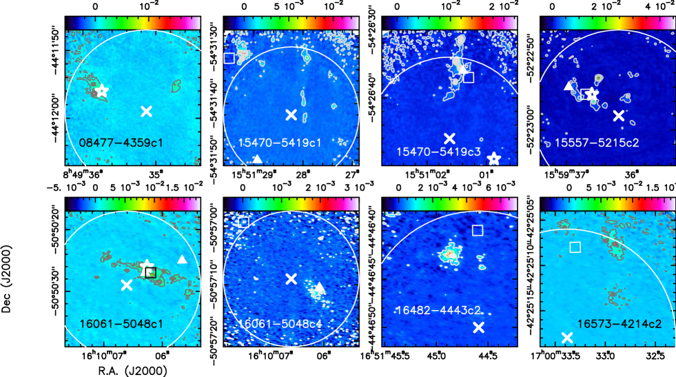
Figure 2: Dust thermal continuum emission maps (contours) at 278 GHz obtained with ALMA with angular resolution of $\sim 0\aas@@fstack{\prime\prime}25$ towards the eight targets detected. All images are primary beam corrected. The wedge on top of each panel indicates the flux density scale (in Jy beam^-1). The target names are reported at the bottom of each frame. Three targets were observed but undetected: 13039–6108c6, 15557–5215c3, and 16435–4515c3. Their maps are shown in Fig. 3. Contours start from the 3$\sigma$ rms level, and are in steps of 10–20$\sigma$ rms, depending on the source. In each panel, the white circle indicates the ALMA field of view at 278 GHz ($\sim$24^′′) centred on the single-dish mm continuum peak marked by the cross (Beltrán et al. 2006). The white stars show the eventual Spitzer 24 $\mu$m continuum peak detected in the ALMA field of view (see Fig. 1), and the filled triangles pinpoint the position of the H₂O maser spots detected towards some clumps (Giannetti et al. 2013). The square shows the emission peak detected in ATLASGAL, at $\sim 870$ $\mu$m (Schuller et al. 2009; source 08477–4359c1 is not present in the ATLASGAL catalogue).

5 Discussion

5.1 Fragment properties versus clump properties

We have searched for possible relations between the properties of the fragment population in Table 2, and the physical parameters of the parent clumps (in Table 1). We have focused on the following clump parameters: gas temperature, total mass, diameter, H₂ total column density, CO depletion factor, non themal velocity dispersion, SFE, and ratio between sound speed and non-thermal velocity dispersion. The non-thermal velocity dispersion, $\sigma_{\rm nth}$, has been estimated from the C¹⁸O (3–2) line width at half maximum by subtracting the thermal contribution (calculated assuming the gas temperature listed in Col. 7 of Table 1). We stress from the beginning that all the conclusions drawn in this Section should be corroborated by a higher statistics. However, some of our findings are indicative of possible correlations that will need to be confirmed with statistically larger samples.

We have first investigated possible relations between the number of fragments and the physical properties of the parent clump. This comparison is shown in Fig. 4: overall, there are no clear (anti-)correlations, although the sources with the largest temperature and mass tend to have more fragments. In particular, with the exception of 16061–5048c4, clumps with more than 200 $M_{\odot}$ always show at least 8 fragments. That the warmer clumps have, on average, more fragments is consistent with the fact that the flux in the less massive fragments is higher if they are warmer. In Fig. 4, we also distinguish between the clumps with and without a 24 $\mu$m source, to check if the presence of the embedded infrared source can influence the fragment population. Again we cannot find any clear difference between the two classes of objects, which could indicate that the star formation activity does not influence the number of fragments (if we assume that the presence of an embedded infrared source indicates a higher star formation activity). This finding is in agreement with Palau et al. (2013), whose study suggested that the evolutionary stage does not have effects on the fragmentation.

We have investigated for possible relations between the mass of the fragments and the clump properties. In Fig. 5, we show the maximum and total mass of the fragments ($m_{\rm max}$ and $m_{\rm tot}$, respectively) as a function of $T$, $\sigma_{\rm nth}$, and the Mach number, i.e. the ratio between the non-thermal velocity dispersion and the sound speed, $\sigma_{\rm nth}/c_{\rm S}$, in order to evaluate the influence of the thermal and turbulent supports. Both $m_{\rm max}$ and $m_{\rm tot}$ increase with $T$ and $\sigma_{\rm nth}$, suggesting that warmer and more turbulent clumps tend to form more massive fragments. In order to evaluate which one is dominant, we have plotted $m_{\rm max}$ and $m_{\rm tot}$ as a function of $\sigma_{\rm nth}/c_{\rm S}$: even though in this case the trend is less apparent, the clumps with higher $\sigma_{\rm nth}/c_{\rm S}$, i.e. with lower thermal support, tend to form more massive objects.

The warmer clumps are also characterised by the largest separation between the fragments, as indicated by Fig. 6, in which we show the maximum linear separation ($S_{\rm max}$) as a function of clump properties. Finally, we have checked for possible trends with the average and maximum clump linear size ($D_{\rm ave}$ and $D_{\rm max}$, respectively), and found again a tentative positive trend with the clump temperature, although this result is quite speculative and certainly needs to be corroborated by a higher statistics.

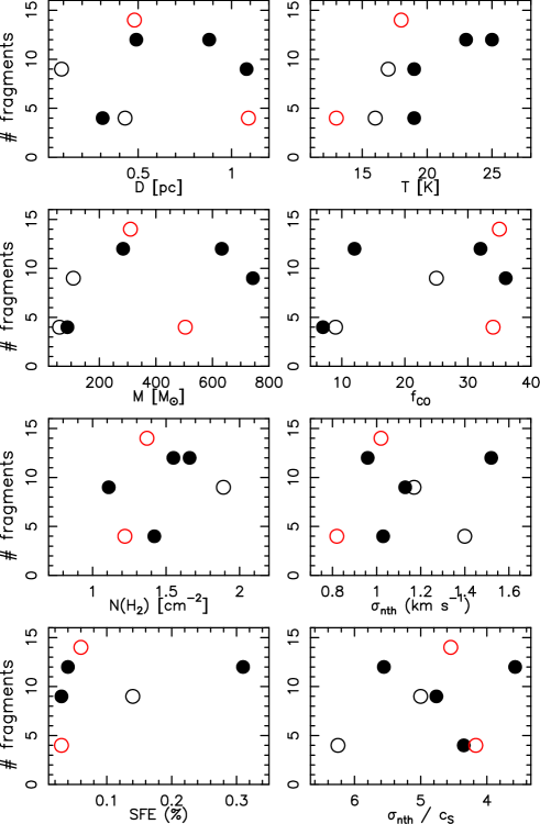
Figure 4: Number of fragments observed per clump (see Tables from A-1 to A-7 versus the following clump parameters: diameter ($D$), mass ($M_{\rm gas}$), H₂ total column density (N(H₂)), SFE, gas temperature ($T$), CO depletion factor ($f_{\rm CO}$), non-thermal velocity dispersion ($\sigma_{\rm nth}$), and the ratio between the non-thermal velocity dispersion and the sound speed ($c_{\rm S}$), i.e. the Mach number. Filled and empty circles indicate clumps with and without an embedded 24$\mu$m source. The red circles corresponds to 15470–5419c1 and 16061–5048c4, in which the interpretation of the clump population needs to be taken with big caution (see Sect. 4.1). In the total H₂ column densities, we have excluded the outlier 16482–4443c2 (see Table 1).

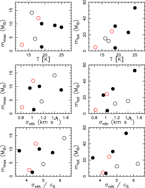
Figure 5: Maximum and total mass of the fragments ($m_{\rm max}$ and $m_{\rm tot}$, respectively) as a function of the clump gas temperature ($T$), the non-thermal velocity dispersion ($\sigma_{\rm nth}$), and the ratio between $\sigma_{\rm nth}$ and the sound speed ($c_{\rm S}$), i.e. the Mach number. The typical uncertainties on the masses, mainly due to the mass opacity coefficient, can be up to a factor 2–3 (see Sect. 4.1).

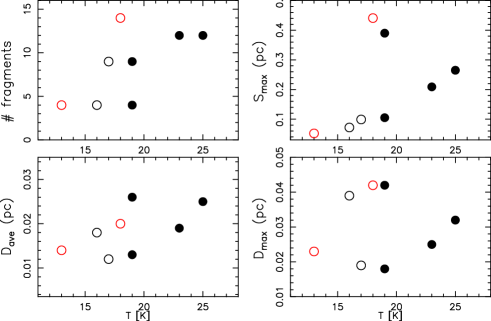
Figure 6: Number, maximum separation ($S_{\rm max}$), average and maximum size of the fragments ($D_{\rm ave}$ and $D_{\rm max}$, respectively) as a function of the clump temperature. The values on the y-axis are not rounded up to the significant digits, and the typical uncertainties on both the diameters and the separations are of about 10$\%$.

5.2 Comparison with numerical simulations

In Fontani et al. (2016), we have simulated the gravitational collapse of 16061–5048c1 through 3D numerical simulations adapted from Commerçon et al. (2011) using the RAMSES code (Teyssier 2002). We consider spherical clouds of radius $r_{0}$ with an initial density profile $\rho(r)=\rho_{\rm c}/(1+(r/r_{\rm c})^{2})$, where $\rho_{\rm c}$ is the central density and $r_{c}$ the extent of the central plateau. In all models, we impose a density contrast of 10 between the center and the border of the cloud. More details about the numerical model can be found in appendix B.1 of Fontani et al. (2016). The calculations were made adopting mass, temperature, average density, and turbulence of the parent clump very similar to those measured in this source with single-dish observations (Beltrán et al. 2006, Fontani et al. 2012, Giannetti et al. 2013). We considered two degrees of magnetisation: $\mu=2$, which is close to the values 2–3 that are observationally inferred (e.g. Crutcher 2012), and $\mu=200$, which corresponds to a quasi-hydrodynamical case. The outcome of the simulations were converted in flux density units of the thermal dust continuum emission using the RADMC-3D radiative transfer code (Dullemond et al. 2012), following the same procedure as in Commerçon et al. (2012a, 2012b). These maps have then been post-processed through the CASA simulator to obtain synthetic images with the same observational conditions as the real observations assuming a source distance of 3.6 kpc and a region of 80 000$\times$80 000 au centred around the most massive protostar. Following the same approach, in this paper we analyse a total of four reference models:

• (1) initial mass of 100 $M_{\odot}$, gas temperature $T=10$ K, Mach number $\mathcal{M}\sim 3$, and virial parameter $\alpha_{\rm vir}=2E_{\rm kin}/E_{\rm grav}=0.4$. The inital density profile is caracterized by $r_{\rm c}=0.22$ pc, $r_{0}=0.67$ pc, and $\rho_{0}=1.4\times 10^{-20}$ g cm^-3. The outcome of these simulations is shown in Fig. 8. Note that these simulations correspond to the ones presented originally in Commerçon et al. (2011), which assume $\mu=130$ for the faint magnetised case. The difference with the $\mu=200$ case, assumed in the other simulations, is completely irrelevant for the fragment population. They have been run without sink particles (e.g. Bleuler & Teyssier 2014), thus without the protostellar radiative feedback;

• (2) initial mass of 300 $M_{\odot}$, gas temperature $T=20$ K, Mach number $\mathcal{M}\sim 6.4$, and virial parameter $\alpha_{\rm vir}=1.1$. The inital density profile is caracterized by $r_{\rm c}=0.085$ pc, $r_{0}=0.25$ pc, and $\rho_{0}=1.5\times 10^{-18}$ g cm^-3. The outcome of these simulations is shown in Fig. 9. These simulations correspond to the ones used in Fontani et al. (2016);

• (3) initial mass of 300 $M_{\odot}$, gas temperature $T=20$ K, Mach number $\mathcal{M}\sim 3$, and virial parameter $\alpha_{\rm vir}=0.22$. The initial density profile is the same as for simulations (2). The outcome of these simulations is shown in Fig. 10;

• (4) initial mass of 300 $M_{\odot}$, gas temperature $T=10$ K, Mach number $\mathcal{M}\sim 6.4$, and virial parameter $\alpha_{\rm vir}=1.1$. The inital density profile is caracterized by $r_{\rm c}=0.17$ pc, $r_{0}=0.5$ pc, and $\rho_{0}=1.9\times 10^{-19}$ g cm^-3. The outcome of these simulations is shown in Fig. 11. In this set of initial conditions, we do not change the ratio between the initial thermal and gravitational energies of simulations (2) and (3). The initial clump is two times larger in radius and the initial density a factor of 8 smaller. Similarly, since the temperature is two times smaller and the Mach number does not change compared to simulations (2), the initial velocity fluctuations are a factor $\sqrt{2}$ smaller in amplitude. Simulations (2), (3), and (4) contain initially the same number of thermal Jeans masses ($\propto T^{3/2}\rho^{-1/2}$);

By comparing simulations (2), (3) and (4), we can understand the separate effect of temperature and turbulence. The source distance assumed in the synthetic images is always 3.6 kpc for the $M=100-300\leavevmode\nobreak\$$M_{\odot}$ cases, which is an average distance of the observed clumps. We have post-processed the simulations as made in Fontani et al. (2016). A set of models that would reproduce the precise initial conditions of each single clump goes far beyond the scope of this paper. In the following, our main aim is to compare the overall morphology of the real and synthetic images to understand if the observed population of fragments is more consistent with strong or with faint magnetic support, and how the initial temperature and turbulence induce clear differences in the population of the fragments. To this purpose, we have decided to analyse the simulations stopped at a SFE of $15\%$, which is an intermediate value between the minimum and maximum SFE found in our sample.

Table 3: Statistical properties of the sink particles when the SFE is $15\%$: absolute time after the start of the simulations, time corresponding to an SFE of 15% after the formation of the first sink particle (time $t_{0}$), number of sink particles, mean and maximum mass of the sink particles, mean and maximum separation between the sink particles, and SFR measured for an SFE $\in[4\%-15\%]$.

Model	$t_{15}$	$t_{15}-t_{0}$	$N_{\rm sink}$	$m_{\rm ave}$	$m_{\rm max}$	$S_{\rm ave}$	$S_{\rm max}$	SFR
	kyr	kyr		$M_{\odot}$	$M_{\odot}$	au	au	$M_{\odot}$ yr-1
$\mu=2$, $T=20$K, $\mathcal{M}=6.4$, $\alpha_{\mathrm{vir}}=1.1$	108	38	36	1.6	7.6	$1\times 10^{4}$	$2.6\times 10^{4}$	$1.5\times 10^{-3}$
$\mu=2$, $T=10$K, $\mathcal{M}=6.4$, $\alpha_{\mathrm{vir}}=1.1$	302	106	47	1.3	6	$2.2\times 10^{4}$	$5.1\times 10^{4}$	$5.3\times 10^{-4}$
$\mu=2$, $T=20$K, $\mathcal{M}=3$, $\alpha_{\mathrm{vir}}=0.22$	98	28	44	1.7	18	$4.5\times 10^{3}$	$1.3\times 10^{4}$	$2.7\times 10^{-3}$
$\mu=200$, $T=20$K, $\mathcal{M}=6.4$, $\alpha_{\mathrm{vir}}=1.1$	84	35	71	0.9	3.3	$1.1\times 10^{4}$	$3.3\times 10^{4}$	$1.7\times 10^{-3}$
$\mu=200$, $T=10$K, $\mathcal{M}=6.4$, $\alpha_{\mathrm{vir}}=1.1$	237	107	84	0.65	3	$2\times 10^{4}$	$6.2\times 10^{4}$	$6.2\times 10^{-4}$
$\mu=200$, $T=20$K, $\mathcal{M}=3$, $\alpha_{\mathrm{vir}}=0.22$	78	27	47	1.4	6.6	$2.3\times 10^{3}$	$1.5\times 10^{4}$	$2.5\times 10^{-3}$

5.2.1 Qualitative description of the simulations

In this section, we briefly describe the outcome of the (2), (3), and (4) sets of simulations. The simulations (1) have been already analysed in Commerçon et al. (2011) and we refer the readers to this work for more details. We focus on the sink particles (i.e., protostars) distribution properties. In the analysis, we select the sink particles with mass larger than $0.1$ $M_{\odot}$. Table 3 reports the sink particles population properties for each simulation when the SFE is $\sim 15\%$. First we note that the time $t_{15}$ at which the SFE reaches 15 % after the start of the simulations depends on all the initial parameters: temperature, magnetisation, and Mach number. Nevertheless, if this time is rescaled after the time $t_{0}$ which corresponds to the time of the first sink particle formation, it does not depend on the magnetisation anymore. This result indicates that even though magnetic fields “dilute” gravity prior to the formation of the first protostars, the subsequent evolution of the SFE is mainly driven by the parent clump properties other than magnetic fields once gravity has taken over. Second, the mean and maximum mass are always largest in the strongly magnetised runs. Except for the $\mathcal{M}\sim 3$ runs, the number of sink particles is almost twice smaller with $\mu=2$, meaning that the strongly magnetised cases favour massive star formation, as already reported in the literature from both models and observations (e.g., Commerçon et al. 2011, Tan et al. 2013, Federrath et al. 2015, Kong et al. 2017, 2018). The mean and maximum separations have been calculated within a spherical region of radius 40000 au around the most massive protostar in order to compare them with the observations. There is no evidence of a correlation of the separation, nor the mean mass with the initial parameters. We also report the measured star formation rate (SFR) which is computed for a SFE varying from 4% to 15%. By comparing simulations (2) and (3), the SFR decreases when $\alpha_{\mathrm{vir}}$ increases as expected from the analytical work in the literature (e.g., Hennebelle & Chabrier 2011). In the runs with $\mathcal{M}\sim 6.4$, the SFR increases by a factor $\sim 2.8$ as the initial temperature is doubled, in line with the total number of protostars. This factor is similar to the factor $\sqrt{8}$ resulting from the difference in the central density free-fall times of simulations (2) and (4) ($t_{\mathrm{ff,(2)}}=t_{\mathrm{ff,(4)}}/\sqrt{8}$), which implies that the SFR measured in unit of the freefall time, i.e., SFR${}_{\mathrm{ff}}=\mathrm{SFR}t_{\mathrm{ff}}(\rho_{\rm c})/M_{0}$ (Krumholz & McKee 2005), remains unchanged.

Figure 7 (left) shows the time evolution of the number of sink particles and of the SFE for simulations (2), (3), and (4), in which the initial mass is 300 $M_{\odot}$. The time evolution has been rescaled after the time $t_{0}$ when the first sink particle was formed. First, we see that the number of protostars in the most turbulent runs ($\mathcal{M}\sim 6.4$) are the most sensitive to the magnetisation. We also note that runs with $\mu=2$ and $\mathcal{M}\sim 6.4$ exhibit a similar slope in the time evolution of the number of protostars. The number of protostars formed in the least turbulent runs $\mathcal{M}\sim 3$ is not dependent on the initial magnetisation. The initial turbulence being weaker, these runs are more dominated by gravity once collapse has been initiated. Interestingly, the SFE does not depend on the magnetisation, while it is sensitive to the initial thermal and turbulent supports as previously mentioned.

Figure 7 (right) shows the time evolution of the mean sink mass and mean separation between sink particles. First, the mean and the maximum protostar mass are always larger in the strongly magnetised run in accordance with previous results of simulations (1). The evolution of the mean separation between protostars shows interesting features. If we focus on the solid lines, i.e., all the sink particles which sit within a sphere of radius 40000 au around the most massive one, we do not find a clear correlation with the initial parameters. The mean separation of the $\mathcal{M}\sim 6.4$ runs is globally smaller for the strongly magnetised case. The dashed line represents the evolution of the mean separation if all the sink particles formed in the simulations are considered. The separation then depends more on the initial temperature and Mach number than on the magnetisation. Focusing on $\mathcal{M}\sim 6.4$ runs, the separation is a factor $\sim 10$ larger in the case of a lower initial temperature, with a maximum separation larger than $80000$ au. This result is consistent with previous studies that show how the fragmentation region extent depends strongly on the initial density profile (e.g., Girichidis et al. 2011). In simulations (4), the inital density profile is flatter than in simulations (2) which favors fragmentation over a wider region. This means that some parts of the simulated clumps where star formation takes place are not taken into account in the synthetic observation we present below. Last but not least, the analysis on the mean separation, averaged over all dimensions, does not reflect the morphology of the fragmentation regions. In Appendix B, we show histrograms of the sink particle separation distribution, as well as their 2D projected distributions for the $\mathcal{M}\sim 6.4$, $T=10$ K runs. A discussion of these distributions is also provided in the same Appendix.

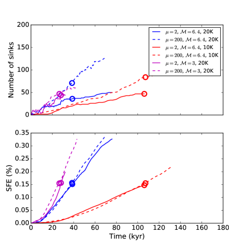
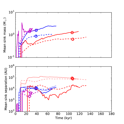
Figure 7: Left: Time evolution of the number of sink particles (top) and of the SFE (bottom) for simulations (2), (3), and (4), i.e. the simulations that reproduce the collapse of a 300 $M_{\odot}$ clump. The circles indicate the time at which we postprocessed the simulations, which corresponds to a SFE$\simeq 15$%. Right: Time evolution of the mean sink particle mass (top) and of the mean separation between sink particles (bottom). The thin lines show the mean separation calculated by accounting for the sink partciles located within a sphere of radius 40 000 au around the most massive one. The dashed lines show the mean separation between all the sink particles.

5.2.2 Qualitative comparison with observations

We now compare our observations with the synthetic images created from the simulations described in the previous Section with the method explained in Fontani et al. (2016). Let us discuss first the case in Fig. 8: assuming a clump mass of 100 $M_{\odot}$, the model is the most appropriate to reproduce the initial conditions of the less massive clumps of our sample, i.e. 08477–4359c1,16482–4443c2, and 16573–4214c2. Depending on $\mu$, the simulations predict either one single fragment in the high magnetic-support case ($\mu=2$), or several fragments packed in a region smaller than $\sim 8000$ au in the other case ($\mu=130$, see bottom panels in Fig. 8). Both predictions are different from our images, because the three clumps mentioned above show all more than one fragment, but these are distributed in an area more extended than 8000 au ($\sim 15000-20000$ au, see Fig. 2 and Col. 8 in Table 2). However, the case that better resembles the images of the less massive sources is the strongly magnetised case, $\mu=2$, because in the $\mu=130$ case, the fragments should have similar size and flux, while in our objects all clumps have a dominant fragment surrounded by much fainter fragments. Moreover, our simulations assume, among the initial conditions, that a single, spherically symmetric clump fragments. Models assuming more complex density profiles such as, e.g., turbulent periodic boxes (e.g. Padoan & Nordlund 2011, Federrath & Klessen 2012, Haugbølle et al. 2018, Mocz et al. 2017), or clouds with more complex turbulent structure (e.g. Li et al. 2018, Girichidis et al. 2011, Federrath et al. 2014, Myers et al. 2014), would provide certainly more fragments. Indeed, our targets could not be single spherical objects, as can be deduced also from the SIMBA maps in Fig. 1. Hence, the initial conditions in our simulations are expected to be those that show the lower level of fragmentation, and the comparison needs to be taken with caution.

The case shown in Fig. 9, especially made to match as well as possible the parameters of 16061–5048c1 in Fontani et al. (2016), can be adopted to qualitatively discuss also 15470–5419c1, 15470–5419c3, and 15557–5215c2. The only difference with Fontani et al. (2016) is that the image that we analyse in this work is obtained when the SFE is $15\%$, while that analysed in Fontani et al. (2016) matched the total flux observed towards 16061–5048c1. For 16061–5048c1, we concluded that the overall filamentary morphology was a strong evidence in favour of the $\mu=2$ case, which cannot be obtained in a weakly magnetised case (Fontani et al. 2016). A filamentary-like shape is found also in 15470–5419c3. The other two sources (15470–5419c1 and 15557–5215c2) show a more irregular structure, which could be explained by a weakly magnetised clump. But even in this case there is not a good agreement, because the fragments predicted by the simulations are distributed in an area less extended than that found in our ALMA images. Moreover, the case of 15470–5419c1 must be interpreted with particular caution because of the huge amount of extended flux resolved out and the location of the most massive fragments at the border of the primary beam.

Figs. 10 and 11 show what happens when we start from a lower Mach number and a lower kinetic temperature, respectively. Inspection of these figures indicates that more than one fragment can be found only if the turbulence is relatively high, because in the $\mathcal{M}=3$ case we find no fragmentation, independent of the magnetic field strength. None of our sources, however, show less than 4 fragments, which implies that this combination of initial conditions is not realistic. This is consistent with the clump velocity dispersions, which indicate always high levels of turbulence. However, as discussed above for the 100 $M_{\odot}$ case, a big caveat arises from the initial density profile adopted in the simulations, which, as stated before, is expected to provide the lower number of fragments and could not be appropriate for our sources if they are not single global spherically symmetric clumps.

To make a more quantitative comparison with the data, we have calculated the properties of the fragments using the same criteria adopted for the real images (see Sect. 4.2). Some statistically relevant quantities are reported in Table 4, and confirm the previous qualitative analysis, namely that: (1) the $\mu=2$ case produces fewer and more massive fragments; (2) more than 1 fragment is possible only if the turbulence is higher ($\mathcal{M}\sim 6.4$ case); (3) the initial temperature has limited influence on the final population of fragments, but warmer clumps tend to exhibit more fragments because the fragmentation region is more concentrated. As shown in figures 7 and B-2, some part of the fragmentation region is missed by our analysis of the synthetic maps of simulations (4) if we consider only the region that would have been observed with ALMA. Overall, the synthetic images discussed in this work allow us to confirm that both the turbulence and the magnetic field are key ingredients in the fragmentation of massive dense clumps, and our observations tend to favour an interplay between turbulence and magnetic field to explain both the morphology and the number of fragments detected.

Table 4: Statistical properties of the fragment population in the synthetic images. The same properties as in Table 2 are shown. The SFE assumed in each simulation is $15\%$.

Model	fragment $n.$	$m_{\rm tot}$	$m_{\rm ave}$	$m_{\rm max}$	$<\frac{m_{\rm max}}{m_{\rm comp}}>$	$D_{\rm ave}$	$D_{\rm max}$	$S_{\rm max}$
		$M_{\odot}$	$M_{\odot}$	$M_{\odot}$		pc	pc	pc - au
$\mu=2$, $T=20$K, $\mathcal{M}=6.4$	9	62	7	26	35	0.023	0.048	0.21 - $\sim 41000$
$\mu=2$, $T=10$K, $\mathcal{M}=6.4$	6	75	12	38	38	0.018	0.026	0.17 - $\sim 33000$
$\mu=2$, $T=20$K, $\mathcal{M}=3$	1	173	–	–	–	0.09	–	–
$\mu=200$, $T=20$K, $\mathcal{M}=6.4$	13	45	3.5	25	24	0.020	0.041	0.21 - $\sim 41000$
$\mu=200$, $T=10$K, $\mathcal{M}=6.4$	11	25	12	13	22	0.013	0.022	0.18 - $\sim 35000$
$\mu=200$, $T=20$K, $\mathcal{M}=3$	1	87	–	–	–	0.083	–	–

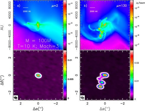
Figure 8: Simulations of the gravitational collapse of a 100 $M_{\odot}$ collapsing clump, with gas temperature $T=10$ K, and Mach number $\mathcal{M}\sim 3$. a): model predictions for the strongly magnetised case, $\mu=2$. In the top panel, we show the direct outcome of the simulations, while the same image processed with the CASA simulator is shown in the bottom panel (first contour and step is 0.3 mJy beam^-1). b): same as a) for the weakly magnetised case, $\mu=130$.

Figure 9: Simulations of the gravitational collapse of a 300 $M_{\odot}$ collapsing clump, with gas temperature $T=20$ K, and Mach number $\mathcal{M}\sim 6.4$. a): model predictions for the strongly magnetised case , $\mu=2$. In the top panel, we show the direct outcome of the simulations, while the same image processed with the CASA simulator is shown in the bottom panel. The first contour is 0.6 mJy beam^-1 as in Fontani et al. (2016, roughly 3 times the 1$\sigma$ rms of most images). The steps are 1.2, 2, 5, 10, 30 and 50 mJy beam^-1. b): same as a) for the weakly magnetised case, $\mu=130$. These simulations have the same set of initial parameters as those discussed in Fontani et al. (2016), but we have post-processed and analysed those at which the star formation efficiency (SFE) is $15\%$, while in Fontani et al. (2016) we analysed the time at which the SFE matched that of IRAS 16061–5048c1 ($\sim 30\%$).

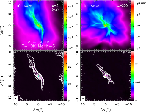
Figure 10: Same as Fig. 9 for a clump with Mach number $\mathcal{M}\sim 3$.

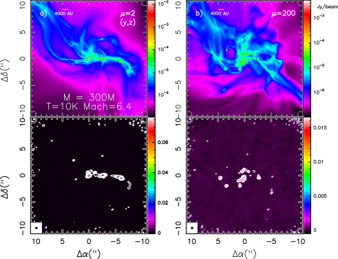
Figure 11: Same as Fig. 9 for a clump with gas temperature $T=10$ K.

6 Conclusions

We have used ALMA to image the 278 GHz continuum emission in 11 massive dense clumps in which the star formation activity is low or absent, to understand the fragment population at the earliest phases of the gravitational collapse. The angular resolution of our observations ($0\aas@@fstack{\prime\prime}25$) is able to resolve a linear scale of $\sim 1000$ au at the distance of the sources. The clumps show a fragment population with at least four fragments distributed in different morphologies, mostly filament-like or irregular. In four targets a dominant fragment surrounded by companions with much smaller mass and size is identified, while many ($\geq 8$) fragments with a gradual change in masses and sizes are found in the others. The number of fragments is likely a lower limit given the huge amount of missing flux in most of the sources. This effect is especially relevant in the targets showing a displacement between the phase centre and the location of the ATLASGAL emission peak. In general, there are no clear relations between the properties of the clumps and those of their fragments, although our results tentatively indicate that the more massive and warmer clumps tend to have more fragments concentrated over a single region. Comparison with the simulations indicate that fragmentation of clumps with initial conditions similar to our objects can occur only assuming a high ($\mathcal{M}\sim 6$) initial turbulence, while in a lower turbulent scenario ($\mathcal{M}\sim 3$) only one very massive fragment surrounded by an extended envelope is expected. Both observations and simulations show that the initially warmer clumps tend to form more fragments. A filament-like morphology is predicted most likely in a highly magnetised clump. We hence conclude that the clumps with many fragments distributed in a filamentary-like structure can be obtained only if the magnetic field plays a dominant role, while the other morphologies are possible also in a weaker magnetised case, or in a scenario in which both magnetic field and turbulence interplay.

Acknowledgments. This paper makes use of the following ALMA data: ADS/JAO.ALMA.2012.1.00366.S. ALMA is a partnership of ESO (representing its member states), NSF (USA) and NINS (Japan), together with NRC (Canada), NSC and ASIAA (Taiwan), and KASI (Republic of Korea), in cooperation with the Republic of Chile. The Joint ALMA Observatory is operated by ESO, AUI/NRAO and NAOJ. We acknowledge the Italian-ARC node for their help in the reduction of the data. We acknowledge partial support from Italian Ministero dell’Istruzione, Universitá e Ricerca through the grant Progetti Premiali 2012 $-$ iALMA (CUP C52I13000140001) and from Gothenburg Centre of Advanced Studies in Science and Technology through the program Origins of habitable planets. ASM is partially supported by the Deutsche Forschungsgemeinschaft (DFG) through grant SFB956 (subproject A6).

Appendix A: Identification and physical properties of the fragments

In Figs. A-1 to  A-7, we show the identified fragments in each source, while in tables A-1 to A-7 we list their main properties: peak position, integrated flux density ($F_{\nu}$), peak flux density ($F_{\nu}^{\rm peak}$), diameter ($D$), and mass ($m$). The coordinates of each fragment indicate the position of its peak flux. The other parameters have beed derived as explained in Sect. 4.2. The map of 16061–5048c1 is not shown because already published in Fontani et al. (2016), following the same approach for the fragment identification.

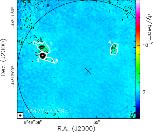
Figure A-1: ALMA dust thermal continuum emission map at 278 GHz towards 08477–4359c1. The first contour level, and the step, is $8.7\times 10^{-4}$ Jy beam^-1, corresponding to the 3$\sigma$ rms noise level ($1\sigma\sim 2.9\times 10^{-4}$ Jy beam^-1). The white polygons indicate the fragments identified on the basis of the criteria described in Sect. 4. In each panel, the circle indicates the ALMA field of view at 278 GHz ($\sim$24^′′), and the cross the phase center, corresponding to the coordinates in Table 1.

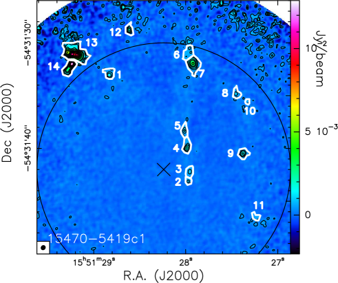
Figure A-2: Same as Fig. A-1 for 15470–5419c1. The first contour level, and the step, is $3.6\times 10^{-4}$ Jy beam^-1, corresponding to the 3$\sigma$ rms noise level ($1\sigma\sim 1.2\times 10^{-4}$ Jy beam^-1).

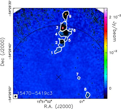
Figure A-3: Same as Fig. A-1 for 15470–5419c3. The first contour level, and the step, is $4.2\times 10^{-4}$ Jy beam^-1, corresponding to the 3$\sigma$ rms noise level ($1\sigma\sim 1.4\times 10^{-4}$ Jy beam^-1).

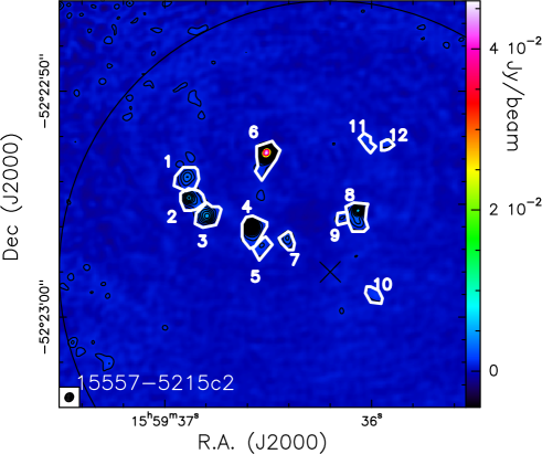
Figure A-4: Same as Fig. A-1 for 15557–5215c2. The first contour level, and the step, is $7.8\times 10^{-4}$ Jy beam^-1, corresponding to the 3$\sigma$ rms noise level ($1\sigma\sim 2.6\times 10^{-4}$ Jy beam^-1).

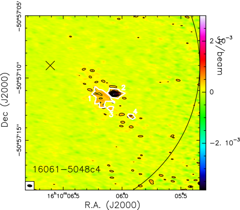
Figure A-5: Same as Fig. A-1 for 16061–5048c4. The first contour level, and the step, is $3\times 10^{-4}$ Jy beam^-1, corresponding to the 3$\sigma$ rms noise level ($1\sigma\sim 1\times 10^{-4}$ Jy beam^-1).

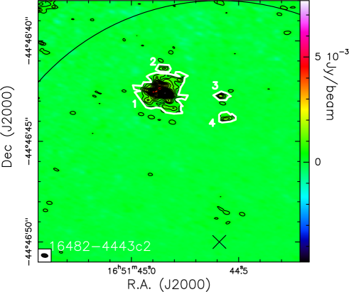
Figure A-6: Same as Fig. A-1 for 16482–4443c2. The first contour level, and the step, is $3\times 10^{-4}$ Jy beam^-1, corresponding to the 3$\sigma$ rms noise level ($1\sigma\sim 1\times 10^{-4}$ Jy beam^-1).

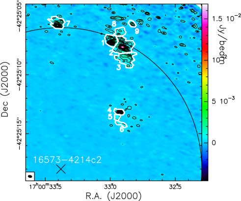
Figure A-7: Same as Fig. A-1 for 16573–4214c2. The first contour level, and the step, is $4.8\times 10^{-4}$ Jy beam^-1, corresponding to the 3$\sigma$ rms noise level ($1\sigma\sim 1.6\times 10^{-4}$ Jy beam^-1).

Table A-1: Peak position (in R.A. and Dec. J2000), integrated flux $F_{\nu}$ (inside the 3$\sigma$ rms contour level), peak flux $F_{\nu}^{\rm peak}$, diameter $D$, and mass $m$ of the fragments identified in Fig. A-1 towards 08477–4359c1. The average error on $F_{\nu}$ is about $1-2\times 10^{-3}$ Jy beam^-1.

Fragment	R.A. (J2000)	Dec. (J2000)	$F_{\nu}$	$F_{\nu}^{\rm peak}$	$D$	$m$
	h:m:s	∘:′:′′	mJy	mJy beam-1	pc	$M_{\odot}$
1	08:49:35.86	$-$44:11:55.1	39	6.11	0.018	1.47
2	08:49:35.85	$-$44:11:56.3	34	19.7	0.011	1.28
3	08:49:35.73	$-$44:11:57.1	6.6	1.40	0.009	0.24
4	08:49:34.74	$-$44:11:55.1	20	2.93	0.014	0.75

Table A-2: Same as Table A-1 for 15470–5419c1.

Fragment	R.A. (J2000)	Dec. (J2000)	$F_{\nu}$	$F_{\nu}^{\rm peak}$	$D$	$m$
	h:m:s	∘:′:′′	mJy	mJy beam-1	pc	$M_{\odot}$
1	15:51:28.83	$-$54:31:33.2	3.0	1.55	0.020	0.63
2	15:51:27.97	$-$54:31:43.2	1.0	0.87	0.013	0.22
3	15:51:27.96	$-$54:31:42.2	2.0	0.94	0.018	0.43
4	15:51:27.98	$-$54:31:40.0	3.8	2.17	0.021	0.80
5	15:51:28.01	$-$54:31:38.4	2.0	1.17	0.017	0.43
6	15:51:27.96	$-$54:31:30.5	3.3	0.85	0.022	0.70
7	15:51:27.92	$-$54:31:32.0	11	4.00	0.029	2.37
8	15:51:27.46	$-$54:31:34.8	1.5	1.02	0.016	0.33
9	15:51:27.38	$-$54:31:40.5	3.1	1.83	0.020	0.65
10	15:51:27.33	$-$54:31:35.6	0.4	0.69	0.010	0.09
11	15:51:27.22	$-$54:31:46.6	1.0	0.63	0.014	0.20
12	15:51:28.61	$-$54:31:28.8	2.4	1.9	0.018	0.51
13	15:51:29.19	$-$54:31:31.1	57.5	10.0	0.042	12.1
14	15:51:29.24	$-$54:31:32.1	21.8	13.0	0.026	4.60

Table A-3: Same as Table A-1 for 15470–5419c3.

Fragment	R.A. (J2000)	Dec. (J2000)	$F_{\nu}$	$F_{\nu}^{\rm peak}$	$D$	$m$
	h:m:s	∘:′:′′	mJy	mJy beam-1	pc	$M_{\odot}$
1	15:51:01.61	$-$54:26:39.6	4.9	1.11	0.027	0.96
2	15:51:01.53	$-$54:26:37.8	19.9	11.5	0.033	3.89
3	15:51:01.51	$-$54:26:34.6	45.6	21.5	0.027	8.91
4	15:51:01.44	$-$54:26:35.6	37.4	9.10	0.042	7.31
5	15:51:01.43	$-$54:26:37.3	1.7	8.4	0.017	0.34
6	15:51:01.29	$-$54:26:35.1	1.2	0.70	0.015	0.23
7	15:51:01.08	$-$54:26:46.1	0.65	0.77	0.011	0.13
8	15:51:00.86	$-$54:26:50.4	3.6	1.38	0.021	0.71
9	15:51:01.43	$-$54:26:31.4	35.3	15.3	0.033	6.90

Table A-4: Same as Table A-1 for 15557–5215c2.

Fragment	R.A. (J2000)	Dec. (J2000)	$F_{\nu}$	$F_{\nu}^{\rm peak}$	$D$	$m$
	h:m:s	∘:′:′′	mJy	mJy beam-1	pc	$M_{\odot}$
1	15:59:36.89	$-$52:22:53.9	7.6	3.1	0.023	1.32
2	15:59:36.88	$-$52:22:54.7	11	5.60	0.022	1.88
3	15:59:36.79	$-$52:22:55.5	12	5.10	0.023	2.02
4	15:59:36.58	$-$52:22:55.9	22	14.0	0.025	3.87
5	15:59:36.53	$-$52:22:56.8	2.9	1.68	0.016	0.51
6	15:59:36.50	$-$52:22:52.7	54	46.0	0.025	9.45
7	15:59:36.41	$-$52:22:56.5	3.0	2.60	0.014	0.52
8	15:59:36.07	$-$52:22:55.3	12	6.1	0.024	2.07
9	15:59:36.14	$-$52:22:55.6	1.6	1.6	0.012	0.28
10	15:59:36.00	$-$52:22:58.9	2.2	1.4	0.015	0.39
11	15:59:36.03	$-$52:22:52.1	1.7	1.3	0.013	0.30
12	15:59:35.93	$-$52:22:52.4	1.4	1.4	0.011	0.19

Table A-5: Same as Table A-1 for 16061–5048c4.

Fragment	R.A. (J2000)	Dec. (J2000)	$F_{\nu}$	$F_{\nu}^{\rm peak}$	$D$	$m$
	h:m:s	∘:′:′′	mJy	mJy beam-1	pc	$M_{\odot}$
1	16:10:06.20	$-$50:57:11.9	7.24	0.60	0.023	1.92
2	16:10:06.07	$-$50:57:11.3	8.80	2.90	0.017	2.33
3	16:10:06.10	$-$50:57:12.4	0.69	0.52	0.007	0.18
4	16:10:05.93	$-$50:57:13.1	0.93	0.68	0.008	0.25

Table A-6: Same as Table A-1 for 16482–4443c2.

Fragment	R.A. (J2000)	Dec. (J2000)	$F_{\nu}$	$F_{\nu}^{\rm peak}$	$D$	$m$
	h:m:s	∘:′:′′	mJy	mJy beam-1	pc	$M_{\odot}$
1	16:51:44.85	$-$44:46:42.6	69.4	7.68	0.038	14.12
2	16:51:44.85	$-$44:46:41.4	1.64	1.05	0.009	0.33
3	16:51:44.58	$-$44:46:42.8	2.27	1.63	0.010	0.46
4	16:51:44.56	$-$44:46:43.9	2.81	1.22	0.012	0.57

Table A-7: Same as Table A-1 for 16573–4214c2.

Fragment	R.A. (J2000)	Dec. (J2000)	$F_{\nu}$	$F_{\nu}^{\rm peak}$	$D$	$m$
	h:m:s	∘:′:′′	mJy	mJy beam-1	pc	$M_{\odot}$
1	17:00:32.99	$-$42:25:07.3	21.3	9.72	0.012	1.96
2	17:00:32.91	$-$42:25:07.6	39.0	17.5	0.015	3.59
3	17:00:32.86	$-$42:25:08.4	21.7	2.42	0.017	2.00
4	17:00:32.92	$-$42:25:13.2	7.88	5.70	0.009	0.73
5	17:00:32.95	$-$42:25:13.6	1.93	0.85	0.006	0.18
6	17:00:32.94	$-$42:25:14.1	2.33	0.84	0.007	0.21
7	17:00:33.41	$-$42:25:05.9	18.6	5.10	0.014	1.71
8	17:00:32.94	$-$42:25:06.6	6.20	1.60	0.011	0.57
9	17:00:32.83	$-$42:25:05.7	3.25	1.80	0.007	0.30

Appendix B: Sink particles distribution in simulations

Figure B-1 shows the histograms of the separation distribution for simulations (2), (3), and (4) along the three coordinates axis. The trend of figure 7 is recovered: the largest separation are found for simulations (4) (middle row) while the smallest one are found in simulations (3) (bottom row). In the $(\mu=2,\mathcal{M}\sim 6.4)$, the separation in the $z$-direction is smaller than in the other two directions, with a difference of a factor $\sim 10$. This means that a filamentary structure with an aspect ratio of 1/10 can be seen by looking at the sink particle distribution in two directions. This feature is only present the strongly magnetized and most turbulent simulations. In all other case, we find a more compact size distribution, suggesting a more roundish sink particle distribution.

Figure B-2 shows the 2D projected sink particles distribution around the most massive one for simulations (3). The red circle delimits the region within a radius of 40000 au that would be observed in our ALMA synthetic observations. A non-negligible number of sink particles is thus excluded from analaysis, and would not be picked up by ALMA in the configuration we used.

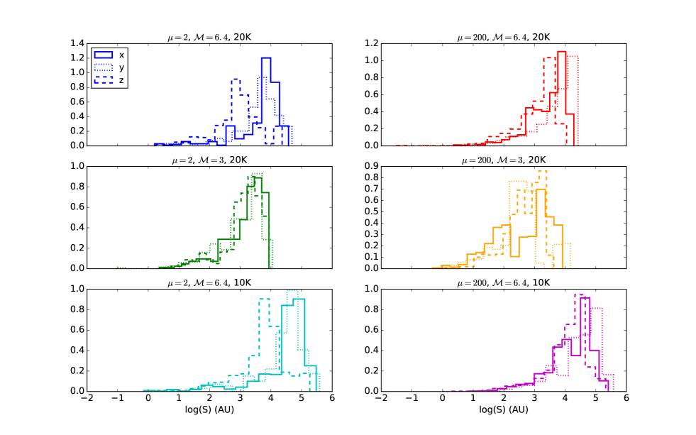
Figure B-1: Histograms of the sink particles separation distribution at a SFE of 15%. The top row shows simulations (2), middle simulations (3), and bottom simulations (4). The left (resp. right) column shows the $\mu=2$ ($\mu=200$) cases. The solid line represents the separation distribution in the $x$-direction, the dotted line that in the $y$-direction, and the dashed line that in the $z$-direction.

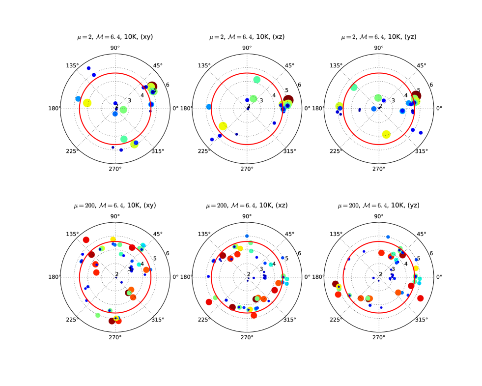
Figure B-2: Projected sink particle distribution centered around the most massive sink particles at an SFE of 15% for simulations (3) ($\mathcal{M}\sim 6.4$, $T=10$ K). The radial direction shows the distance in au in logarithmic scale. The red circle represents the size of the region that we post-processed with CASA to produce the ALMA synthetic observations.

References

- Bate (2009) Bate, M.R. 2009, MNRAS, 392, 1363
- Beltrán et al. (2006) Beltrán, M.T., Brand, J., Cesaroni, R., Fontani, F., Pezzuto, S. et al. 2006, A&A, 447, 221
- Beltrán et al. (2013) Beltrán, M.T., Olmi, L., Cesaroni, R., Schisano, E., Elia, D. et al. 2013, A&A, 552, 123
- Beuther et al. (2002) Beuther, H., Schilke, P., Sridharan, T.K., Menten, K.M., Walmsley, C.M., Wyrowski, F. 2002, A&A, 566, 945
- Bleuler et al. (2014) Bleuler, A., Teyssier, R. 2014, MNRAS, 445, 4015
- Bonnell et al. (2004) Bonnell, I.A., Vine, S.G., Bate M.R. 2004, MNRAS, 349, 735
- Bontemps et al. (2010) Bontemps, S., Motte, F., Csengeri, T., Schneider, N. 2010, A&A, 524, 18
- Caselli et al. (1999) Caselli, P., Walmsley, C.M., Tafalla, M., Dore, L., Myers, P. 1999, ApJ, 523, L165
- Commerçon et al. (2011) Commerçon, B., Hennebelle, P., Henning, T. 2011, ApJ, 742, L9
- Commerçon et al. (2012a) Commerçon, B., Launhardt, R., Dullemond, C., Henning, Th. 2012a, A&A, 545, 98
- Commerçon et al. (2012b) Commerçon, B., Levrier, F., Maury, A.J., Henning, Th., Launhardt, R. 2012b, A&A, 548, 39
- Commerçon et al. (2014) Commerçon, B., Debout, V., Teyssier, R. 2014, A&A, 563, 11
- Crutcher (2012) Crutcher, R.M. 2013, ARA&A, 50, 29
- Csengeri et al. (2017) Csengeri, T., Bontemps, S., Wyrowski, F., Motte, F., Menten, K.M. et al. 2017, A&A, 600, L10
- Cyganowski et al. (2017) Cyganowski, C.J., Brogan, C.L., Hunter, T.R., Smith, R., Kruijssen, J.M.D., Bonnell, I.A., Zhang, Q. 2017, MNRAS, 468, 3694
- Dobbs et al. (2005) Dobbs, C.L., Bonnell, I.A., Clark, P.C. 2005, MNRAS, 360, 2
- Dullemond et al. (2012) Dullemond, C.P., Juhasz, A., Pohl, A., Sereshti, F., Shetty, R., Peters, T., Commerçon, B., Flock, M. 2012, Astrophysics Source Code Library
- Emprechtinger et al. (2009) Emprechtinger, M., Caselli, P., Volgenau, N.H., Stutzki, J., Wiedner, M.C. 2009, A&A, 493, 89
- Federrath (2015) Federrath, C. 2015, MNRAS, 450, 4035
- Federrath et al. (2014) Federrath, C., Schrön, M., Banerjee, R., Klessen, R.S. 2014, ApJ, 790, 128
- Federrath & Klessen (2012) Federrath, C., & Klessen, R.S. 2012, ApJ, 761, 156
- Fontani et al. (2005) Fontani, F., Beltrán, M.T., Brand, J., Cesaroni, R., Molinari, S. et al. 2005, A&A, 432, 921
- Fontani et al. (2012) Fontani, F., Giannetti, A., Beltrán, M.T., Dodson, R., Rioja, M. et al. 2012, MNRAS, 423, 2342
- Fontani et al. (2016) Fontani, F., Commerçon, B., Giannetti, A., Beltrán, M.T., Sánchez-Monge, Á., et al. 2016, A&A, 593, L14
- Fromang et al. (2006) Fromang, S., Hennebelle, P., Teyssier, R. 2006, A&A, 457, 371
- Giannetti et al. (2013) Giannetti, A., Brand, J., Sanchez-Monge, Á., Fontani, F., Cesaroni, R. et al. 2013, A&A, 556, 16
- Girichidis et al. (2011) Girichidis, P., Federrath, C., Banerjee, R., Klessen, R. S. 2011, MNRAS, 413, 2741
- Haugbølle et al. (2018) Haugbølle, T., Padoan, P, Nordlund, A., 2018, arXiv:170901078
- Hennebelle et al. (2011) Hennebelle, P., Commerçon, B., Joos, M., Klessen, R.S., Krumholz, M., Tan, J.C., Teyssier, R. 2011, A&A, 528, 72
- Hennebelle & Chabrier (2011) Hennebelle, P. & Chabrier, G. 2011, ApJ, 743, L29
- Henshaw et al. (2017) Henshaw, J.D., Jiménez-Serra, I., Longmore, S.N., Caselli, P., Pineda, J.E., et al. 2017, MNRAS, 464, L31
- Kauffmann & Pillai (2010) Kauffmann, J. & Pillai, T. 2010, ApJ, 723, L7
- Kauffmann et al. (2017) Kauffmann, J., Goldsmith, P.F., Melnick, G., Tolls, V., Guzman, A., Menten, K.M. 2017, A&A, 605, L5
- Kong et al. (2017) Kong, S., Tan, J.C., Caselli, P., Fontani, F., Liu, M., Butler, M.J. 2017, ApJ, 834, 193
- Kong et al. (2018) Kong, S., Tan, J.C., Caselli, P., Fontani, F., Wang, K., Butler, M.J. 2018, arXiv:170105953
- Krumholz (2005) Krumholz, M.R. & McKee, C.F. 2005, ApJ, 630, 250
- Krumholz (2006) Krumholz, M.R. 2006, ApJ, 641, L45
- Krumholz et al. (2009) Krumholz, M.R., Klein, R., McKee, C.F., Offner, S.S.R., Cunningham, A.J.A. 2009, Science, 323, 754
- Krumholz et al. (2014) Krumholz, M.R., Bate, M.R., Arce, H.G., Dale, J.E., Gutermuth, R. et al. 2014, Protostars and Planets VI, H. Beuther, R.S. Klessen, C.P. Dullemond, and Th. Henning (eds.), 914, 243
- Li et al. (2018) Li, P.S., Klein, R.I., McKee, C.F. 2018, MNRAS, 473, 4220
- Longmore et al. (2011) Longmore, S.N., Pillai, T., Keto, E., Zhang, Q., Qiu, K. 2011, ApJ, 726, L97
- Lopez-Sepulcre et al. (2010) Lopez-Sepulcre, A., Cesaroni, R., Walmsley, C.M. 2010, A&A, 517, 66
- Maret et al. (maret) Maret, S., Hily-Blant, P., Pety, J., Bardeau, S., Reynier, E. 2011, A&A, 526, 47
- McKee & Tan (2003) McKee, C. & Tan, J.C. 2003, ApJ, 585, 850
- McMullin et al. (2007) McMullin, J.P., Waters, B., Schiebel, D., Young, W., & Golap, K. 2007, in Astronomical Data Analysis Software and Systems XVI, eds. R. A. Shaw, F. Hill, & D. J. Bell, ASP Conf. Ser., 376, 127
- Mocz et al. (2017) Mocz, P., Burkhart, B., Hernquist, L., McKee, C.F., Springel, V. 2017, ApJ, 838, 40
- Mouschovias & Spitzer (1976) Mouschovias, T.C. & Spitzer, L.J. ApJ, 210, 326
- Myers et al. (2014) Myers, A.T., Klein, R.I., Krumholz, M.R., McKee, C.F. 2014, MNRAS, 439, 3420
- Ossenkopf & Henning (1994) Ossenkopf, V., & Henning, T. 1994, A&A, 291, 943
- Padoan & Nordlund (2011) Padoan, P. & Nordlund, Å 2011, ApJ, 730, 40
- Palau et al. (2013) Palau, A., Fuente, A., Girart, J.M., Estalella, R., Ho, P.T.P., Sánchez-Monge, A., et al. 2013, ApJ, 762, 120
- Palau et al. (2015) Palau, A., Ballesteros-Paredes, J., Vázquez-Semadeni, E., Sánchez-Monge, Á., Estalella, R., et al. 2015, MNRAS, 453, 3785
- Palau et al. (2017) Palau, A., Zapata, A.L., Román-Zúñiga, C.G., Sánchez-Monge, A., Estalella, R., et al. 2017, arXiv: 1706.04623
- Peretto et al. (2013) Peretto, N., Fuller, G.A., Duarte-Cabral, A., Avison, A., Hennebelle, P., et al. 2013, A&A, 555, 112
- Pillai et al. (2015) Pillai, T., Kauffmann, J., Tan, J.C., Goldsmith, P.F., Carey, S.J., Menten, K.M. 2015, ApJ, 799, 74
- Pineda et al. (2009) Pineda, J.E., Rosolowsky, E.W., Goodman, A.A. 2009, ApJ, 699, L134
- Ragan et al. (2011) Ragan, S.E., Bergin, E.A., Wilner, D. 2011, ApJ, 736, 163
- Rathborne et al. (2015) Rathborne, J.M., Longmore, S.N., Jackson, J.M., Alves, J.F., Bally, J., et al. 2015, ApJ, 802, 125
- Sanchez-Monge et al. (2013) Sanchez-Monge, Á, Beltrán, M.T., Cesaroni, R., Fontani, F., Brand, et al. 2013, A&A, 550, 21
- Schuller et al. (2009) Schuller, F., Menten, K.M., Contreras, Y., Wyrowski, F., Schilke, P., et al. 2009, A&A, 504, 415
- Tan et al. (2013) Tan, J.C., Kong, S., Butler, M.J., Caselli, P., Fontani, F. 2013, ApJ, 779, 96
- Teyssier (2002) Teyssier, R. 2002, A&A, 385, 337
- Weiss et al. (2005) Weiss, A., Hillebrandt, W., Thomas, H.-C., Ritter, H. 2005, Book review: Cox and Giuli’s Principles of Stellar Structure, Cambridge, UK: Princeton Publishing Associates Ltd
- Zhang et al. (2015) Zhang, Q., Wang, K., Xing, L., Jiménez-Serra, I. 2015, ApJ, 804, 141