An Accelerated Directional Derivative Method for Smooth Stochastic Convex Optimization

Pavel Dvurechensky  Eduard Gorbunov  Alexander Gasnikov This paper was published in European Journal of Operational Research (DOI: https://doi.org/10.1016/j.ejor.2020.08.027).
P. Dvurechensky (pavel.dvurechensky@wias-berlin.de) is with Weierstrass Institute for Applied Analysis and Stochastics and Institute for Information Transmission Problems RAS. E. Gorbunov (eduard.gorbunov@phystech.edu, eduardgorbunov.github.io) is with Moscow Institute of Physics and Technology and National Research University Higher School of Economics. A. Gasnikov (gasnikov@yandex.ru) is with Moscow Institute of Physics and Technology, National Research University Higher School of Economics and Institute for Information Transmission Problems RAS
(August 20, 2020)
Abstract

We consider smooth stochastic convex optimization problems in the context of algorithms which are based on directional derivatives of the objective function. This context can be considered as an intermediate one between derivative-free optimization and gradient-based optimization. We assume that at any given point and for any given direction, a stochastic approximation for the directional derivative of the objective function at this point and in this direction is available with some additive noise. The noise is assumed to be of an unknown nature, but bounded in the absolute value. We underline that we consider directional derivatives in any direction, as opposed to coordinate descent methods which use only derivatives in coordinate directions. For this setting, we propose a non-accelerated and an accelerated directional derivative method and provide their complexity bounds. Our non-accelerated algorithm has a complexity bound which is similar to the gradient-based algorithm, that is, without any dimension-dependent factor. Our accelerated algorithm has a complexity bound which coincides with the complexity bound of the accelerated gradient-based algorithm up to a factor of square root of the problem dimension. We extend these results to strongly convex problems.

1 Introduction

Zero-order or derivative-free optimization considers problems of minimization of a function using only, possibly noisy, observations of its values. This area of optimization has a long history, starting as early as in 1960 [64, 34], see also [17, 67, 23]. Even an older area of optimization, which started in 19th century [19], considers first-order methods which use the information about the gradient of the objective function. In this paper, we choose an intermediate class of problems. Namely, we assume that at any given point and for any given direction, a noisy stochastic approximation for the directional derivative of the objective function at this point in this direction is available. We underline that we consider directional derivatives in any direction, as opposed to coordinate descent methods which rely only on derivatives in coordinate directions. We refer to the class of optimization methods, which use directional derivatives of the objective function, as directional derivative methods. Unlike well developed areas of derivative-free and first-order stochastic optimization methods, the area of directional derivative optimization methods for stochastic optimization problems is not sufficiently covered in the literature. This class of optimization methods can be motivated by at least three situations.

The first one is connected to Automatic Differentiation [71]. Assume that the objective function is given as a computer program, which performs elementary arithmetic operations and elementary functions evaluations. Automatic Differentiation allows to calculate the gradient of this objective function and the additional computational cost is no more than five times larger than the cost of the evaluation of the objective value. The drawback of this approach is that it requires to store in memory the result of all the intermediate operations, which can require large memory amount. On the contrary, calculation of the directional derivative is easier than the calculation of the full gradient and requires the same memory amount as the calculation of the value of the objective [49]. Since a random vector can be a part of the program input or some randomness can be used during the program execution, stochastic optimization problems can also be considered.

Importantly, automatic calculation of the directional derivative does not require the objective function to be smooth. This fact motivates the study of directional derivative methods in connection to Deep Learning. Indeed, learning problem is often stated as a problem of minimization of a loss function. A non-smooth activation function, called rectifier, is frequently used in Deep Learning as a building block for the loss function. Formally speaking, this non-smoothness does not allow to use Automatic Differentiation in the form of backpropagation to calculate the gradient of the objective function. At the same time, directional derivatives can be calculated by properly modified backpropagation.

The second motivating situation is connected to quasi-variational inequalities, which are used in modelling of different phenomena, such as sandpile formation and growth [63], determination of lakes and river networks [6], and superconductivity [5]. It happens that directional derivatives can be calculated for such problems [54] as a solution to some auxiliary problem. Since this subproblem can not always be solved exactly, the noise in the directional derivative naturally arises. If the considered physical phenomenon takes place in some random media, stochastic optimization can be a natural approach to use.

The third motivating situation is connected to derivative-free stochastic optimization. In this situation a gradient approximation, based on the difference of stochastic approximations for the values of the objective in two close points, can be considered as a noisy directional derivative in the direction given by the difference of these two points [33]. In this case, derivative-free stochastic optimization can be considered as a particular case of directional derivative stochastic optimization.

Motivated by potential presence of non-stochastic noise in the problem, we assume that the noise in the directional derivative consists of two parts. Similar to stochastic optimization problems, the first part is of a stochastic nature. On the opposite, the second part is an additive noise of an unknown nature, but bounded in the absolute value. More precisely, we consider the following optimization problem

minxn{f(x):=𝔼ξ[F(x,ξ)]=𝒳F(x,ξ)𝑑P(x)},subscript𝑥superscript𝑛assign𝑓𝑥subscript𝔼𝜉delimited-[]𝐹𝑥𝜉subscript𝒳𝐹𝑥𝜉differential-d𝑃𝑥\min_{x\in\mathbb{R}^{n}}\left\{f(x):=\mathbb{E}_{\xi}[F(x,\xi)]=\int_{\mathcal{X}}F(x,\xi)dP(x)\right\}, (1)

where ξ𝜉\xi is a random vector with probability distribution P(ξ)𝑃𝜉P(\xi), ξ𝒳𝜉𝒳\xi\in\mathcal{X}, and for P𝑃P-almost every ξ𝒳𝜉𝒳\xi\in\mathcal{X}, the function F(x,ξ)𝐹𝑥𝜉F(x,\xi) is closed and convex. Moreover, we assume that, for P𝑃P almost every ξ𝜉\xi, the function F(x,ξ)𝐹𝑥𝜉F(x,\xi) has gradient g(x,ξ)𝑔𝑥𝜉g(x,\xi), which is L(ξ)𝐿𝜉L(\xi)-Lipschitz continuous with respect to the Euclidean norm and there exists L20subscript𝐿20L_{2}\geqslant 0 such that 𝔼ξL(ξ)2L2<+subscript𝔼𝜉𝐿superscript𝜉2subscript𝐿2\sqrt{\mathbb{E}_{\xi}L(\xi)^{2}}\leqslant L_{2}<+\infty. Under this assumptions, 𝔼ξg(x,ξ)=f(x)subscript𝔼𝜉𝑔𝑥𝜉𝑓𝑥\mathbb{E}_{\xi}g(x,\xi)=\nabla f(x) and f𝑓f has L2subscript𝐿2L_{2}-Lipschitz continuous gradient with respect to the Euclidean norm. Also we assume that

𝔼ξ[g(x,ξ)f(x)22]σ2,subscript𝔼𝜉delimited-[]superscriptsubscriptnorm𝑔𝑥𝜉𝑓𝑥22superscript𝜎2\mathbb{E}_{\xi}[\|g(x,\xi)-\nabla f(x)\|_{2}^{2}]\leqslant\sigma^{2}, (2)

where 2\|\cdot\|_{2} is the Euclidean norm.

Finally, we assume that an optimization procedure, given a point xn𝑥superscript𝑛x\in\mathbb{R}^{n}, direction eS2(1)𝑒subscript𝑆21e\in S_{2}(1) and ξ𝜉\xi independently drawn from P𝑃P, can obtain a noisy stochastic approximation f~(x,ξ,e)superscript~𝑓𝑥𝜉𝑒\widetilde{f}^{\prime}(x,\xi,e) for the directional derivative g(x,ξ),e𝑔𝑥𝜉𝑒\langle g(x,\xi),e\rangle:

f~(x,ξ,e)superscript~𝑓𝑥𝜉𝑒\displaystyle\widetilde{f}^{\prime}(x,\xi,e) =g(x,ξ),e+ζ(x,ξ,e)+η(x,ξ,e),absent𝑔𝑥𝜉𝑒𝜁𝑥𝜉𝑒𝜂𝑥𝜉𝑒\displaystyle=\langle g(x,\xi),e\rangle+\zeta(x,\xi,e)+\eta(x,\xi,e),
𝔼ξ(ζ(x,ξ,e))2subscript𝔼𝜉superscript𝜁𝑥𝜉𝑒2\displaystyle\mathbb{E}_{\xi}(\zeta(x,\xi,e))^{2} Δζ,xn,eS2(1),formulae-sequenceabsentsubscriptΔ𝜁formulae-sequencefor-all𝑥superscript𝑛for-all𝑒subscript𝑆21\displaystyle\leqslant\Delta_{\zeta},\;\forall x\in\mathbb{R}^{n},\forall e\in S_{2}(1),
|η(x,ξ,e)|𝜂𝑥𝜉𝑒\displaystyle|\eta(x,\xi,e)| Δη,xn,eS2(1),a.s. in ξ,formulae-sequenceabsentsubscriptΔ𝜂formulae-sequencefor-all𝑥superscript𝑛for-all𝑒subscript𝑆21a.s. in 𝜉\displaystyle\leqslant\Delta_{\eta},\;\forall x\in\mathbb{R}^{n},\forall e\in S_{2}(1),\;\text{a.s. in }\xi, (3)

where S2(1)subscript𝑆21S_{2}(1) is the Euclidean sphere or radius one with the center at the point zero and the values ΔζsubscriptΔ𝜁\Delta_{\zeta}, ΔηsubscriptΔ𝜂\Delta_{\eta} are controlled and can be made as small as it is desired. Note that we use the smoothness of F(,ξ)𝐹𝜉F(\cdot,\xi) to write the directional derivative as g(x,ξ),e𝑔𝑥𝜉𝑒\langle g(x,\xi),e\rangle, but we do not assume that the whole stochastic gradient g(x,ξ)𝑔𝑥𝜉g(x,\xi) is available.

It is well-known [50, 25, 31, 36] that, if the stochastic approximation g(x,ξ)𝑔𝑥𝜉g(x,\xi) for the gradient of f𝑓f is available, an accelerated gradient method has complexity bound O(max{L2/ε,σ2/ε2})𝑂subscript𝐿2𝜀superscript𝜎2superscript𝜀2O\left(\max\left\{\sqrt{L_{2}/\varepsilon},\sigma^{2}/\varepsilon^{2}\right\}\right), where ε𝜀\varepsilon is the target optimization error. The question, to which we give a positive answer in this paper, is as follows.

Is it possible to solve a smooth stochastic optimization problem with the same ε𝜀\varepsilon-dependence in the complexity and only noisy observations of the directional derivative?

1.1 Related work

We first consider the related work on directional derivative optimization methods and, then, a closely related class of derivative-free methods with two-point feedback, the latter meaning that an optimization method uses two function value evaluations on each iteration. Since all the considered methods are randomized, we compare oracle complexity bounds in terms of expectation, that is, a number of directional derivatives or function values evaluations which is sufficient to achieve an error ε𝜀\varepsilon in the expected optimization error 𝔼f(x^)f𝔼𝑓^𝑥superscript𝑓\mathbb{E}f(\hat{x})-f^{*}, where x^^𝑥\hat{x} is the output of an algorithm and fsuperscript𝑓f^{*} is the optimal value of f𝑓f.

1.1.1 Directional derivative methods

Deterministic smooth optimization problems. In [60], the authors consider the Euclidean case and propose a non-accelerated and an accelerated directional derivative method for smooth convex problems with complexity bounds O(nL2/ε)𝑂𝑛subscript𝐿2𝜀O(nL_{2}/\varepsilon) and O(nL2/ε)𝑂𝑛subscript𝐿2𝜀O(n\sqrt{L_{2}/\varepsilon}) respectively. Also they propose a non-accelerated and an accelerated method for problems with μ𝜇\mu-strongly convex objective and prove complexity bounds O(nL2/μlog2(1/ε))𝑂𝑛subscript𝐿2𝜇subscript21𝜀O(nL_{2}/\mu\log_{2}(1/\varepsilon)) and O(nL2/μlog2(1/ε))𝑂𝑛subscript𝐿2𝜇subscript21𝜀O(n\sqrt{L_{2}/\mu}\log_{2}(1/\varepsilon)) respectively. For a more general case of problems with additional bounded noise in directional derivatives, but also for the Euclidean case, an accelerated directional derivative method was proposed in [33] and a bound O(nL2/ε)𝑂𝑛subscript𝐿2𝜀O(n\sqrt{L_{2}/\varepsilon}) was proved.

We also should mention coordinate descent methods. In the seminal paper [57], a random coordinate descent for smooth convex and μ𝜇\mu-strongly convex optimization problems were proposed and O(L/ε)𝑂𝐿𝜀O(L/\varepsilon) and O(L/μlog2(1/ε))𝑂𝐿𝜇subscript21𝜀O(L/\mu\log_{2}(1/\varepsilon)) complexity bounds were proved, where L𝐿L is an effective Lipschitz constant of the gradient varying from n𝑛n to some average over coordinates coordinate-wise Lipschitz constant. In the same paper, an accelerated version of random coordinate descent was proposed for convex problems and O(nL/ε)𝑂𝑛𝐿𝜀O(n\sqrt{L/\varepsilon}) complexity bound was proved. Papers [52, 35, 53, 65] generalize accelerated random coordinate descent for different settings, including μ𝜇\mu-strongly convex problems, and [61, 3, 41] provide a O(L/ε)𝑂𝐿𝜀O(\sqrt{L/\varepsilon}) and O(L/μlog2(1/ε))𝑂𝐿𝜇subscript21𝜀O(\sqrt{L/\mu}\log_{2}(1/\varepsilon)) complexity bounds, where L𝐿L is an effective Lipschitz constant of the gradient varying from n𝑛n to some average over coordinates coordinate-wise Lipschitz constant, and, in the best case, is dimension-independent. An accelerated random coordinate descent with inexact coordinate-wise derivatives was proposed in [33] with O(nL/ε)𝑂𝑛𝐿𝜀O(n\sqrt{L/\varepsilon}) complexity bound and also a unified view on directional derivative methods, coordinate descent and derivative-free methods.

Stochastic optimization problems. A directional derivative method for non-smooth stochastic convex optimization problems was introduced in [60] with a complexity bound O(n2/ε2)𝑂superscript𝑛2superscript𝜀2O(n^{2}/\varepsilon^{2}). A random coordinate descent method for non-smooth stochastic convex and μ𝜇\mu- strongly convex optimization problems were introduced in [24] with complexity bounds O(n/ε2)𝑂𝑛superscript𝜀2O(n/\varepsilon^{2}) and O(n/με)𝑂𝑛𝜇𝜀O(n/\mu\varepsilon) respectively.

1.1.2 Derivative-free methods

Deterministic smooth optimization problems. A non-accelerated and an accelerated derivative-free method for this type of problems were proposed in [60] for the Euclidean case with the bounds O(nL2/ε)𝑂𝑛subscript𝐿2𝜀O(nL_{2}/\varepsilon) and O(nL2/ε)𝑂𝑛subscript𝐿2𝜀O(n\sqrt{L_{2}/\varepsilon}) respectively. The same paper proposed a non-accelerated and an accelerated method for μ𝜇\mu-strongly convex problems with complexity bounds O(nL2/μlog2(1/ε))𝑂𝑛subscript𝐿2𝜇subscript21𝜀O(nL_{2}/\mu\log_{2}(1/\varepsilon)) and O(nL2/μlog2(1/ε))𝑂𝑛subscript𝐿2𝜇subscript21𝜀O(n\sqrt{L_{2}/\mu}\log_{2}(1/\varepsilon)) respectively. A non-accelerated derivative-free method for deterministic problems with additional bounded noise in function values was proposed in [15] together with O(nL2/ε)𝑂𝑛subscript𝐿2𝜀O(nL_{2}/\varepsilon) bound and application to learning parameter of a parametric PageRank model, see also [38, 37]. Deterministic problems with additional bounded noise in function values were also considered in [33], where several accelerated derivative-free methods, including Derivative-Free Block-Coordinate Descent, were proposed and a bound O(nL/ε)𝑂𝑛𝐿𝜀O(n\sqrt{L/\varepsilon}) was proved, where L𝐿L depends on the method and, in some sense, characterizes the average over blocks of coordinates Lipschitz constant of the derivative in the block. Mixed first-order/zero-order setting is considered in [13]. After our paper appeared as a preprint, the papers [10, 16] studied derivative-free quasi-Newton methods for problems with noisy function values, and the paper [11] reported theoretical and empirical comparison of different gradient approximations for zero-order methods.

Stochastic optimization problems. Most of the authors in this group solve a more general problem of bandit convex optimization and obtain bounds on the so-called regret. It is well known [20] that a bound on the regret can be converted to a bound on the expected optimization error. Non-smooth stochastic optimization problems were considered in [60], where an O(n2/ε2)𝑂superscript𝑛2superscript𝜀2O(n^{2}/\varepsilon^{2}) complexity bound was proved for a derivative-free method. This bound was improved by [26, 40, 39, 66, 8, 46] to111O~~𝑂\widetilde{O} hides polylogarithmic factors (lnn)csuperscript𝑛𝑐(\ln n)^{c}, c>0𝑐0c>0. O~(n2/qRp2/ε2)~𝑂superscript𝑛2𝑞superscriptsubscript𝑅𝑝2superscript𝜀2\widetilde{O}(n^{2/q}R_{p}^{2}/\varepsilon^{2}), where p{1,2}𝑝12p\in\{1,2\}, 1p+1q=11𝑝1𝑞1\frac{1}{p}+\frac{1}{q}=1 and Rpsubscript𝑅𝑝R_{p} is the radius of the feasible set in the p𝑝p-norm p\|\cdot\|_{p}. For non-smooth μpsubscript𝜇𝑝\mu_{p}-strongly convex w.r.t. to p𝑝p-norm problems, the authors of [39, 8] proved a bound O~(n2/q/(μpε))~𝑂superscript𝑛2𝑞subscript𝜇𝑝𝜀\widetilde{O}(n^{2/q}/(\mu_{p}\varepsilon)). A version of these methods for non-smooth saddle-point problems is developed in [14].

Intermediate, partially smooth problems with a restrictive assumption of boundedness of 𝔼g(x,ξ)2𝔼superscriptnorm𝑔𝑥𝜉2\mathbb{E}~{}\|g(x,\xi)\|^{2}, were considered in [26], where it was proved that a proper modification of Mirror Descent algorithm with derivative-free approximation of the gradient gives a bound O(n2/qRp2/ε2)𝑂superscript𝑛2𝑞superscriptsubscript𝑅𝑝2superscript𝜀2O(n^{2/q}R_{p}^{2}/\varepsilon^{2}) for convex problems, improving upon the bound O~(n2/ε2)~𝑂superscript𝑛2superscript𝜀2\widetilde{O}(n^{2}/\varepsilon^{2}) of [1]. For strongly convex w.r.t 222-norm problems, the authors of [1] obtained a bound O~(n2/ε)~𝑂superscript𝑛2𝜀\widetilde{O}(n^{2}/\varepsilon), which was later extended for μpsubscript𝜇𝑝\mu_{p}-strongly convex problems and improved to O~(n2/q/(μpε))~𝑂superscript𝑛2𝑞subscript𝜇𝑝𝜀\widetilde{O}(n^{2/q}/(\mu_{p}\varepsilon)) in [39].

In the fully smooth case, without the assumption that 𝔼g(x,ξ)2<+𝔼superscriptnorm𝑔𝑥𝜉2\mathbb{E}\|g(x,\xi)\|^{2}<+\infty, papers [43, 42] proposed a derivative-free algorithm for the Euclidean case with the bound

O~(max{nL2R2ε,nσ2ε2}).~𝑂𝑛subscript𝐿2subscript𝑅2𝜀𝑛superscript𝜎2superscript𝜀2\widetilde{O}\left(\max\left\{\frac{nL_{2}R_{2}}{\varepsilon},\frac{n\sigma^{2}}{\varepsilon^{2}}\right\}\right).

In [45], the authors proposed a non-accelerated and an accelerated derivative-free method with the bounds

O~(max{n2qL2Rp2ε,n2qσ2Rp2ε2}),O~(max{n12+1qL2Rp2ε,n2qσ2Rp2ε2})~𝑂superscript𝑛2𝑞subscript𝐿2superscriptsubscript𝑅𝑝2𝜀superscript𝑛2𝑞superscript𝜎2superscriptsubscript𝑅𝑝2superscript𝜀2~𝑂superscript𝑛121𝑞subscript𝐿2superscriptsubscript𝑅𝑝2𝜀superscript𝑛2𝑞superscript𝜎2superscriptsubscript𝑅𝑝2superscript𝜀2\widetilde{O}\left(\max\left\{\frac{n^{\frac{2}{q}}L_{2}R_{p}^{2}}{\varepsilon},\frac{n^{\frac{2}{q}}\sigma^{2}R_{p}^{2}}{\varepsilon^{2}}\right\}\right),\quad\widetilde{O}\left(\max\left\{n^{\frac{1}{2}+\frac{1}{q}}\sqrt{\frac{L_{2}R_{p}^{2}}{\varepsilon}},\frac{n^{\frac{2}{q}}\sigma^{2}R_{p}^{2}}{\varepsilon^{2}}\right\}\right)

respectively, where Rpsubscript𝑅𝑝R_{p} characterizes the distance in p𝑝p-norm between the starting point of the algorithm and a solution to (1), p{1,2}𝑝12p\in\{1,2\} and q{2,}𝑞2q\in\{2,\infty\} is the conjugate to p𝑝p, given by the identity 1p+1q=11𝑝1𝑞1\frac{1}{p}+\frac{1}{q}=1.

The authors of [21] combine accelerated derivative-free optimization with accelerated variance reduction technique for finite-sum convex problems in the Euclidean setup.

Other works. For a recent review of derivative-free optimization see [51] and for a review of stochastic optimization, including derivative-free optimization, see [62].

1.2 Our contributions

As we have seen above, only two results on directional derivative methods for non-smooth stochastic convex optimization are available in the literature, and, to the best of our knowledge, nothing is known about directional derivative methods for smooth stochastic convex optimization, even in the well-developed area of random coordinate descent methods. Our main contribution consists in closing this gap in the theory of directional derivative methods for stochastic optimization and considering even more general setting with additional noise of an unknown nature in the directional derivative.

Our methods are based on two proximal setups [9] characterized by the value222Strictly speaking, we are able to consider all the intermediate cases p[1,2]𝑝12p\in[1,2], but we are not aware of any proximal setup which is compatible with p{1,2}𝑝12p\notin\{1,2\} p{1,2}𝑝12p\in\{1,2\} and its conjugate q{2,}𝑞2q\in\{2,\infty\}, given by the identity 1p+1q=11𝑝1𝑞1\frac{1}{p}+\frac{1}{q}=1. The case p=1𝑝1p=1 corresponds to the choice of 111-norm in nsuperscript𝑛\mathbb{R}^{n} and corresponding prox-function which is strongly convex with respect to this norm (we provide the details below). The case p=2𝑝2p=2 corresponds to the choice of the Euclidean 222-norm in nsuperscript𝑛\mathbb{R}^{n} and squared Euclidean norm as the prox-function. As our main contribution, we propose an Accelerated Randomized Directional Derivative (ARDD) algorithm for smooth stochastic optimization based on noisy observations of directional derivative of the objective. Our method has the complexity bound

O~(max{n12+1qL2Rp2ε,n2qσ2Rp2ε2}),~𝑂superscript𝑛121𝑞subscript𝐿2superscriptsubscript𝑅𝑝2𝜀superscript𝑛2𝑞superscript𝜎2superscriptsubscript𝑅𝑝2superscript𝜀2\widetilde{O}\left(\max\left\{n^{\frac{1}{2}+\frac{1}{q}}\sqrt{\frac{L_{2}R_{p}^{2}}{\varepsilon}},\frac{n^{\frac{2}{q}}\sigma^{2}R_{p}^{2}}{\varepsilon^{2}}\right\}\right), (4)

where Rpsubscript𝑅𝑝R_{p} characterizes the distance in p𝑝p-norm between the starting point of the algorithm and a solution to (1).

As our second contribution, we propose a non-accelerated Randomized Directional Derivative (RDD) algorithm with the complexity bound

O~(max{n2qL2Rp2ε,n2qσ2Rp2ε2}).~𝑂superscript𝑛2𝑞subscript𝐿2superscriptsubscript𝑅𝑝2𝜀superscript𝑛2𝑞superscript𝜎2superscriptsubscript𝑅𝑝2superscript𝜀2\widetilde{O}\left(\max\left\{\frac{n^{\frac{2}{q}}L_{2}R_{p}^{2}}{\varepsilon},\frac{n^{\frac{2}{q}}\sigma^{2}R_{p}^{2}}{\varepsilon^{2}}\right\}\right). (5)

Interestingly, for this method when p=1𝑝1p=1 and q=𝑞q=\infty, we obtain complexity bound which depends on the dimension n𝑛n only logarithmically despite we use only noisy directional derivative observations. Let us comment on the comparison between the accelerated and non-accelerated method. In the regime of small variance σ2superscript𝜎2\sigma^{2} in both bounds the dominating term is the first one. If p=1𝑝1p=1, q=𝑞q=\infty and L2Rp2<nεsubscript𝐿2superscriptsubscript𝑅𝑝2𝑛𝜀L_{2}R_{p}^{2}<n\varepsilon, then the bound for the non-accelerated method is smaller than that of for the accelerated. In this regime it is preferred to use the non-accelerated method.

Note that, in the case of (1) having a sparse solution, our bounds for p=1𝑝1p=1 allow to gain a factor of n𝑛\sqrt{n} in the complexity of the accelerated method and a factor of n𝑛n in the complexity of the non-accelerated method in comparison to the Euclidean case p=2𝑝2p=2. Indeed, sparsity of a solution xsuperscript𝑥x^{*} means that x1=O(1)x2subscriptnormsuperscript𝑥1𝑂1subscriptnormsuperscript𝑥2\|x^{*}\|_{1}=O(1)\cdot\|x^{*}\|_{2} and, if the starting point is zero, we obtain R12=x12=O(1)x22=O(1)R22superscriptsubscript𝑅12superscriptsubscriptnormsuperscript𝑥12𝑂1superscriptsubscriptnormsuperscript𝑥22𝑂1superscriptsubscript𝑅22R_{1}^{2}=\|x^{*}\|_{1}^{2}=O(1)\cdot\|x^{*}\|_{2}^{2}=O(1)R_{2}^{2}. Hence, the bounds for p=1𝑝1p=1 and p=2𝑝2p=2 can be compared only based on the corresponding powers of n𝑛n, the latter being smaller for the case p=1𝑝1p=1, q=𝑞q=\infty.

We underline here that our methods are based on random directions drawn from the uniform distribution on the unit Euclidean sphere and our results for p=1𝑝1p=1 can not be obtained by random coordinate descent.

As our third contribution, we extend the above results to the case when the objective function is additionally known to be μpsubscript𝜇𝑝\mu_{p}-strongly convex w.r.t. p𝑝p-norm. For this case, we propose an accelerated and a non-accelerated algorithm which respectively have complexity bounds

O~(max{n12+1qL2μplog2μpRp2ε,n2qσ2μpε}),O~(max{n2qL2μplog2μpRp2ε,n2qσ2μpε}).~𝑂superscript𝑛121𝑞subscript𝐿2subscript𝜇𝑝subscript2subscript𝜇𝑝superscriptsubscript𝑅𝑝2𝜀superscript𝑛2𝑞superscript𝜎2subscript𝜇𝑝𝜀~𝑂superscript𝑛2𝑞subscript𝐿2subscript𝜇𝑝subscript2subscript𝜇𝑝superscriptsubscript𝑅𝑝2𝜀superscript𝑛2𝑞superscript𝜎2subscript𝜇𝑝𝜀\widetilde{O}\left(\max\left\{n^{\frac{1}{2}+\frac{1}{q}}\sqrt{\frac{L_{2}}{\mu_{p}}}\log_{2}\frac{\mu_{p}R_{p}^{2}}{\varepsilon},\frac{n^{\frac{2}{q}}\sigma^{2}}{\mu_{p}\varepsilon}\right\}\right),\quad\widetilde{O}\left(\max\left\{\frac{n^{\frac{2}{q}}L_{2}}{\mu_{p}}\log_{2}\frac{\mu_{p}R_{p}^{2}}{\varepsilon},\frac{n^{\frac{2}{q}}\sigma^{2}}{\mu_{p}\varepsilon}\right\}\right). (6)

In the regime of small variance σ2superscript𝜎2\sigma^{2} in both bounds the dominating term is the first one. If p=1𝑝1p=1, q=𝑞q=\infty and L2μp<nsubscript𝐿2subscript𝜇𝑝𝑛\frac{L_{2}}{\mu_{p}}<n, then the bound for the non-accelerated method is smaller than that of for the accelerated. In this regime of relatively well-conditioned problems it is preferred to use the non-accelerated method.

As our final contribution, we consider derivative-free smooth stochastic convex optimization with inexact values of the stochastic approximations for the function values as a particular case of optimization using noisy directional derivatives. This allows us to obtain the complexity bounds of [45] as a straightforward corollary of our results in this paper. At the same time we obtain new complexity bounds for the strongly convex case which, to the best of our knowledge, were not known in the literature.

Note that our results for accelerated and non-accelerated methods are somewhat similar to the finite-sum minimization problems of the form

minxni=1mfi(x),subscript𝑥superscript𝑛superscriptsubscript𝑖1𝑚subscript𝑓𝑖𝑥\min_{x\in\mathbb{R}^{n}}\sum_{i=1}^{m}f_{i}(x),

where fisubscript𝑓𝑖f_{i} are convex smooth functions. For such problems accelerated methods have complexity O~(m+mL/ε)~𝑂𝑚𝑚𝐿𝜀\widetilde{O}(m+\sqrt{mL/\varepsilon}) and non-accelerated methods have complexity O~(m+L/ε)~𝑂𝑚𝐿𝜀\widetilde{O}(m+L/\varepsilon) (see, e.g. [2] for a nice review on the topic). As we see, acceleration allows to take the square root of the second term but for the price of m𝑚\sqrt{m} and the two bounds can not be directly compared without additional assumptions on the value of mε𝑚𝜀m\varepsilon.

Special note on [45, 70]. One of the novelties and insights in the approach of this paper in comparison to [45, 70] is to realize that gradient-free methods are a particular case of directional derivative methods with inexact oracle. Unlike these papers, in the current paper we need to account for two types of inexactness. One is stochastic with bounded second moment and the second is bounded a.s. This is a more complicated assumption than the one in [45, 70] and we have to assume that the error values can be controlled, unlike [45, 70]. Moreover, since the oracle returns different information, we have to construct our stochastic approximation of the gradient differently, which also changes the proof technique. We also analyze in this paper the case of strongly convex objective values, which was not done in [45, 70].

1.3 Paper organization

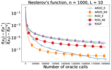
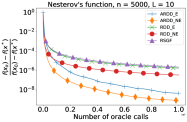
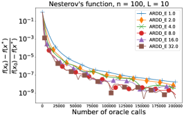
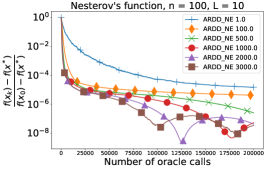
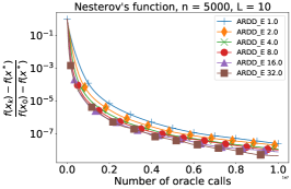
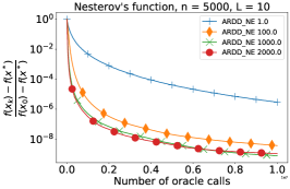
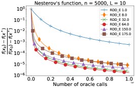
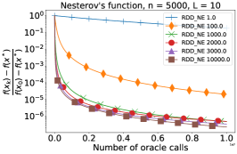
The rest of the paper is organized as follows. In Section 2, both for convex and strongly convex problems, we introduce our algorithms, state their convergence rate theorems and corresponding complexity bounds. Section 3 is devoted to proof of the convergence rate theorem for our accelerated method and convex objective functions. Section 4 is devoted to proof of the convergence rate theorem for our non-accelerated method and convex objective functions. In Section 5 we provide the proofs for the case of strongly convex objective function. Finally, in Section 6 we provide numerical experiments with two types of objective functions: worst case functions for first-order methods [56] and least squares problem.

2 Algorithms and main results

In this section, we provide our non-accelerated and accelerated directional derivative methods both for convex and strongly convex problems together with convergence theorems and corresponding complexity bounds. The proofs are rather technical and postponed to next sections.

2.1 Preliminaries

We start by introducing necessary objects and technical results.

Proximal setup. Let p[1,2]𝑝12p\in[1,2] and xpsubscriptnorm𝑥𝑝\|x\|_{p} be the p𝑝p-norm in nsuperscript𝑛\mathbb{R}^{n} defined as

xpp=i=1n|xi|p,xn,formulae-sequencesuperscriptsubscriptnorm𝑥𝑝𝑝superscriptsubscript𝑖1𝑛superscriptsubscript𝑥𝑖𝑝𝑥superscript𝑛\|x\|_{p}^{p}=\sum\limits_{i=1}^{n}|x_{i}|^{p},\quad x\in\mathbb{R}^{n},

q\|\cdot\|_{q} be its dual, defined by gq=maxx{g,x,xp1}subscriptnorm𝑔𝑞subscript𝑥𝑔𝑥subscriptnorm𝑥𝑝1\|g\|_{q}=\max\limits_{x}\big{\{}\langle g,x\rangle,\|x\|_{p}\leq 1\big{\}}, where q[2,]𝑞2q\in[2,\infty] is the conjugate number to p𝑝p, given by 1p+1q=11𝑝1𝑞1\frac{1}{p}+\frac{1}{q}=1, and, for q=𝑞q=\infty, by definition x=maxi=1,,n|xi|subscriptnorm𝑥subscript𝑖1𝑛subscript𝑥𝑖\|x\|_{\infty}=\max\limits_{i=1,\ldots,n}|x_{i}|.

We choose a prox-function d(x)𝑑𝑥d(x) which is continuous, convex on nsuperscript𝑛\mathbb{R}^{n} and is 111-strongly convex on nsuperscript𝑛\mathbb{R}^{n} with respect to p\|\cdot\|_{p}, i.e., for any x,yn𝑥𝑦superscript𝑛x,y\in\mathbb{R}^{n} d(y)d(x)d(x),yx12yxp2𝑑𝑦𝑑𝑥𝑑𝑥𝑦𝑥12superscriptsubscriptnorm𝑦𝑥𝑝2d(y)-d(x)-\langle\nabla d(x),y-x\rangle\geq\frac{1}{2}\|y-x\|_{p}^{2}. Without loss of generality, we assume that minxnd(x)=0subscript𝑥superscript𝑛𝑑𝑥0\min\limits_{x\in\mathbb{R}^{n}}d(x)=0. We define also the corresponding Bregman divergence V[z](x)=d(x)d(z)d(z),xz𝑉delimited-[]𝑧𝑥𝑑𝑥𝑑𝑧𝑑𝑧𝑥𝑧V[z](x)=d(x)-d(z)-\langle\nabla d(z),x-z\rangle, x,zn𝑥𝑧superscript𝑛x,z\in\mathbb{R}^{n}. Note that, by the strong convexity of d𝑑d,

V[z](x)12xzp2,x,zn.formulae-sequence𝑉delimited-[]𝑧𝑥12superscriptsubscriptnorm𝑥𝑧𝑝2𝑥𝑧superscript𝑛V[z](x)\geq\frac{1}{2}\|x-z\|_{p}^{2},\quad x,z\in\mathbb{R}^{n}. (7)

For the case p=1𝑝1p=1, we choose the following prox-function [9]

d(x)=en(κ1)(2κ)/κlnn2xκ2,κ=1+1lnnformulae-sequence𝑑𝑥esuperscript𝑛𝜅12𝜅𝜅𝑛2superscriptsubscriptnorm𝑥𝜅2𝜅11𝑛d(x)=\frac{{\rm e}n^{(\kappa-1)(2-\kappa)/\kappa}\ln n}{2}\|x\|_{\kappa}^{2},\quad\kappa=1+\frac{1}{\ln n} (8)

and, for the case p=2𝑝2p=2, we choose the prox-function to be the squared Euclidean norm

d(x)=12x22.𝑑𝑥12superscriptsubscriptnorm𝑥22d(x)=\frac{1}{2}\|x\|_{2}^{2}. (9)

Main technical lemma. In our proofs of complexity bounds, we rely on the following lemma. The proof is rather technical and is provided in the appendix.

Lemma 2.1.

Let eRS2(1)𝑒𝑅subscript𝑆21e\in RS_{2}(1), i.e be a random vector uniformly distributed on the surface of the unit Euclidean sphere in nsuperscript𝑛\mathbb{R}^{n}, p[1,2]𝑝12p\in[1,2] and q𝑞q be given by 1p+1q=11𝑝1𝑞1\frac{1}{p}+\frac{1}{q}=1. Then, for n8𝑛8n\geqslant 8 and ρn=min{q1, 16lnn8}n2q1subscript𝜌𝑛𝑞116𝑛8superscript𝑛2𝑞1\rho_{n}=\min\{q-1,\,16\ln n-8\}n^{\frac{2}{q}-1},

𝔼eeq2ρn,subscript𝔼𝑒superscriptsubscriptnorm𝑒𝑞2subscript𝜌𝑛\mathbb{E}_{e}\|e\|_{q}^{2}\leq\rho_{n}, (10)
𝔼e(s,e2eq2)6ρnns22,sn.formulae-sequencesubscript𝔼𝑒superscript𝑠𝑒2superscriptsubscriptnorm𝑒𝑞26subscript𝜌𝑛𝑛superscriptsubscriptnorm𝑠22for-all𝑠superscript𝑛\mathbb{E}_{e}\left(\langle s,e\rangle^{2}\|e\|_{q}^{2}\right)\leq\frac{6\rho_{n}}{n}\|s\|_{2}^{2},\quad\forall s\in\mathbb{R}^{n}. (11)

Stochastic approximation of the gradient. Based on the noisy stochastic observations (3) of the directional derivative, we form the following stochastic approximation of f(x)𝑓𝑥\nabla f(x)

~mf(x)=1mi=1mf~(x,ξi,e)e,superscript~𝑚𝑓𝑥1𝑚superscriptsubscript𝑖1𝑚superscript~𝑓𝑥subscript𝜉𝑖𝑒𝑒\widetilde{\nabla}^{m}f(x)=\frac{1}{m}\sum\limits_{i=1}^{m}\widetilde{f}^{\prime}(x,\xi_{i},e)e, (12)

where eRS2(1)𝑒𝑅subscript𝑆21e\in RS_{2}(1), ξisubscript𝜉𝑖\xi_{i}, i=1,,m𝑖1𝑚i=1,...,m are independent realizations of ξ𝜉\xi, m𝑚m is the batch size.

2.2 Algorithms and main results for convex problems

Our Accelerated Randomized Directional Derivative (ARDD) method is listed as Algorithm 1.

Algorithm 1 Accelerated Randomized Directional Derivative (ARDD) method
0:  x0subscript𝑥0x_{0} —starting point; N1𝑁1N\geqslant 1 — number of iterations; m1𝑚1m\geqslant 1 — batch size.
0:  point yNsubscript𝑦𝑁y_{N}.
1:  y0x0,z0x0formulae-sequencesubscript𝑦0subscript𝑥0subscript𝑧0subscript𝑥0y_{0}\leftarrow x_{0},\,z_{0}\leftarrow x_{0}.
2:  for k=0,,N1𝑘0𝑁1k=0,\,\dots,\,N-1do
3:     αk+1k+296n2ρnL2,τk148αk+1n2ρnL2=2k+2formulae-sequencesubscript𝛼𝑘1𝑘296superscript𝑛2subscript𝜌𝑛subscript𝐿2subscript𝜏𝑘148subscript𝛼𝑘1superscript𝑛2subscript𝜌𝑛subscript𝐿22𝑘2\alpha_{k+1}\leftarrow\frac{k+2}{96n^{2}\rho_{n}L_{2}},\,\tau_{k}\leftarrow\frac{1}{48\alpha_{k+1}n^{2}\rho_{n}L_{2}}=\frac{2}{k+2}.
4:     Generate ek+1RS2(1)subscript𝑒𝑘1𝑅subscript𝑆21e_{k+1}\in RS_{2}(1) independently from previous iterations and ξisubscript𝜉𝑖\xi_{i}, i=1,,m𝑖1𝑚i=1,...,m – independent realizations of ξ𝜉\xi.
5:     Calculate
~mf(xk+1)=1mi=1mf~(xk+1,ξi,e)e.superscript~𝑚𝑓subscript𝑥𝑘11𝑚superscriptsubscript𝑖1𝑚superscript~𝑓subscript𝑥𝑘1subscript𝜉𝑖𝑒𝑒\widetilde{\nabla}^{m}f(x_{k+1})=\frac{1}{m}\sum\limits_{i=1}^{m}\widetilde{f}^{\prime}(x_{k+1},\xi_{i},e)e.
6:     xk+1τkzk+(1τk)yksubscript𝑥𝑘1subscript𝜏𝑘subscript𝑧𝑘1subscript𝜏𝑘subscript𝑦𝑘x_{k+1}\leftarrow\tau_{k}z_{k}+(1-\tau_{k})y_{k}.
7:     yk+1xk+112L2~mf(xk+1)subscript𝑦𝑘1subscript𝑥𝑘112subscript𝐿2superscript~𝑚𝑓subscript𝑥𝑘1y_{k+1}\leftarrow x_{k+1}-\frac{1}{2L_{2}}\widetilde{\nabla}^{m}f(x_{k+1}).
8:     zk+1argminzn{αk+1n~mf(xk+1),zzk+V[zk](z)}subscript𝑧𝑘1subscript𝑧superscript𝑛subscript𝛼𝑘1𝑛superscript~𝑚𝑓subscript𝑥𝑘1𝑧subscript𝑧𝑘𝑉delimited-[]subscript𝑧𝑘𝑧z_{k+1}\leftarrow\mathop{\arg\!\min}\limits_{z\in\mathbb{R}^{n}}\left\{{\alpha_{k+1}n\left\langle\widetilde{\nabla}^{m}f(x_{k+1}),\,z-z_{k}\right\rangle+V[z_{k}]\left(z\right)}\right\}.
9:  end for
10:  return  yNsubscript𝑦𝑁y_{N}
Theorem 2.2.

Let ARDD method be applied to solve problem (1). Then

𝔼[f(yN)]f(x)384Θpn2ρnL2N2+4NnL2σ2m+61N24L2Δζ+122N3L2Δη2+122nΘpN2(Δζ2+2Δη)+N212nρnL2(Δζ2+2Δη)2,𝔼delimited-[]𝑓subscript𝑦𝑁𝑓superscript𝑥384subscriptΘ𝑝superscript𝑛2subscript𝜌𝑛subscript𝐿2superscript𝑁24𝑁𝑛subscript𝐿2superscript𝜎2𝑚61𝑁24subscript𝐿2subscriptΔ𝜁122𝑁3subscript𝐿2superscriptsubscriptΔ𝜂2missing-subexpression122𝑛subscriptΘ𝑝superscript𝑁2subscriptΔ𝜁22subscriptΔ𝜂superscript𝑁212𝑛subscript𝜌𝑛subscript𝐿2superscriptsubscriptΔ𝜁22subscriptΔ𝜂2missing-subexpression\begin{array}[]{rl}\mathbb{E}[f(y_{N})]-f(x^{*})\leqslant\frac{384\Theta_{p}n^{2}\rho_{n}L_{2}}{N^{2}}+\frac{4N}{nL_{2}}\cdot\frac{\sigma^{2}}{m}+\frac{61N}{24L_{2}}\Delta_{\zeta}+\frac{122N}{3L_{2}}\Delta_{\eta}^{2}\\ +\frac{12\sqrt{2n\Theta_{p}}}{N^{2}}\left(\frac{\sqrt{\Delta_{\zeta}}}{2}+2\Delta_{\eta}\right)+\frac{N^{2}}{12n\rho_{n}L_{2}}\left(\frac{\sqrt{\Delta_{\zeta}}}{2}+2\Delta_{\eta}\right)^{2},\end{array} (13)

where Θp=V[z0](x)subscriptΘ𝑝𝑉delimited-[]subscript𝑧0superscript𝑥\Theta_{p}=V[z_{0}](x^{*}) is defined by the chosen proximal setup and 𝔼[]=𝔼e1,,eN,ξ1,1,,ξN,m[]𝔼delimited-[]subscript𝔼subscript𝑒1subscript𝑒𝑁subscript𝜉11subscript𝜉𝑁𝑚delimited-[]\mathbb{E}[\cdot]=\mathbb{E}_{e_{1},\ldots,e_{N},\xi_{1,1},\ldots,\xi_{N,m}}[\cdot].

Before we proceed to the non-accelerated method, we give the appropriate choice of the ARDD method parameters N𝑁N, m𝑚m, and accuracy of the directional derivative evaluation ΔζsubscriptΔ𝜁\Delta_{\zeta}, ΔηsubscriptΔ𝜂\Delta_{\eta}. These values are chosen such that the r.h.s. of (13) is smaller than ε𝜀\varepsilon. For simplicity we omit numerical constants and summarize the obtained values of the algorithm parameters in Table 1 below. The last row represents the total number Nm𝑁𝑚Nm of oracle calls, that is, the number of directional derivative evaluations, which was advertised in (4). Note that the bound (13) allows also to choose the accuracy of the directional derivative evaluation ΔζsubscriptΔ𝜁\Delta_{\zeta}, ΔηsubscriptΔ𝜂\Delta_{\eta} decreasing with N𝑁N. This is done by making each term with ΔζsubscriptΔ𝜁\Delta_{\zeta} or ΔηsubscriptΔ𝜂\Delta_{\eta} in the r.h.s. to be of the same order as the first term.

p=1𝑝1p=1 p=2𝑝2p=2
N𝑁N O(nlnnL2Θ1ε)𝑂𝑛𝑛subscript𝐿2subscriptΘ1𝜀O\left(\sqrt{\frac{n\ln nL_{2}\Theta_{1}}{\varepsilon}}\right) O(n2L2Θ2ε)𝑂superscript𝑛2subscript𝐿2subscriptΘ2𝜀O\left(\sqrt{\frac{n^{2}L_{2}\Theta_{2}}{\varepsilon}}\right)
m𝑚m O(max{1,lnnnσ2ε3/2Θ1L2})𝑂1𝑛𝑛superscript𝜎2superscript𝜀32subscriptΘ1subscript𝐿2O\left(\max\left\{1,\sqrt{\frac{\ln n}{n}}\cdot\frac{\sigma^{2}}{\varepsilon^{3/2}}\cdot\sqrt{\frac{\Theta_{1}}{L_{2}}}\right\}\right) O(max{1,σ2ε3/2Θ2L2})𝑂1superscript𝜎2superscript𝜀32subscriptΘ2subscript𝐿2O\left(\max\left\{1,\frac{\sigma^{2}}{\varepsilon^{3/2}}\cdot\sqrt{\frac{\Theta_{2}}{L_{2}}}\right\}\right)
ΔζsubscriptΔ𝜁\Delta_{\zeta} O(min{n(lnn)2L22Θ1,ε2nΘ1,ε32nlnnL2Θ1})𝑂𝑛superscript𝑛2superscriptsubscript𝐿22subscriptΘ1superscript𝜀2𝑛subscriptΘ1superscript𝜀32𝑛𝑛subscript𝐿2subscriptΘ1O\left(\min\left\{n(\ln n)^{2}L_{2}^{2}\Theta_{1},\,\frac{\varepsilon^{2}}{n\Theta_{1}},\,\frac{\varepsilon^{\frac{3}{2}}}{\sqrt{n\ln n}}\cdot\sqrt{\frac{L_{2}}{\Theta_{1}}}\right\}\right) O(min{n3L22Θ2,ε2nΘ2,ε32nL2Θ2})𝑂superscript𝑛3superscriptsubscript𝐿22subscriptΘ2superscript𝜀2𝑛subscriptΘ2superscript𝜀32𝑛subscript𝐿2subscriptΘ2O\left(\min\left\{n^{3}L_{2}^{2}\Theta_{2},\,\frac{\varepsilon^{2}}{n\Theta_{2}},\,\frac{\varepsilon^{\frac{3}{2}}}{n}\cdot\sqrt{\frac{L_{2}}{\Theta_{2}}}\right\}\right)
ΔηsubscriptΔ𝜂\Delta_{\eta} O(min{nlnnL2Θ1,εnΘ1,ε34nlnn4L2Θ14})𝑂𝑛𝑛subscript𝐿2subscriptΘ1𝜀𝑛subscriptΘ1superscript𝜀344𝑛𝑛4subscript𝐿2subscriptΘ1O\left(\min\left\{\sqrt{n}\ln nL_{2}\sqrt{\Theta_{1}},\,\frac{\varepsilon}{\sqrt{n\Theta_{1}}},\,\frac{\varepsilon^{\frac{3}{4}}}{\sqrt[4]{n\ln n}}\cdot\sqrt[4]{\frac{L_{2}}{\Theta_{1}}}\right\}\right) O(min{n32L2Θ2,εnΘ2,ε34nL2Θ24})𝑂superscript𝑛32subscript𝐿2subscriptΘ2𝜀𝑛subscriptΘ2superscript𝜀34𝑛4subscript𝐿2subscriptΘ2O\left(\min\left\{n^{\frac{3}{2}}L_{2}\sqrt{\Theta_{2}},\,\frac{\varepsilon}{\sqrt{n\Theta_{2}}},\,\frac{\varepsilon^{\frac{3}{4}}}{\sqrt{n}}\cdot\sqrt[4]{\frac{L_{2}}{\Theta_{2}}}\right\}\right)
O-le calls O(max{nlnnL2Θ1ε,σ2Θ1lnnε2})𝑂𝑛𝑛subscript𝐿2subscriptΘ1𝜀superscript𝜎2subscriptΘ1𝑛superscript𝜀2O\left(\max\left\{\sqrt{\frac{n\ln nL_{2}\Theta_{1}}{\varepsilon}},\frac{\sigma^{2}\Theta_{1}\ln n}{\varepsilon^{2}}\right\}\right) O(max{n2L2Θ2ε,σ2Θ2nε2})𝑂superscript𝑛2subscript𝐿2subscriptΘ2𝜀superscript𝜎2subscriptΘ2𝑛superscript𝜀2O\left(\max\left\{\sqrt{\frac{n^{2}L_{2}\Theta_{2}}{\varepsilon}},\frac{\sigma^{2}\Theta_{2}n}{\varepsilon^{2}}\right\}\right)
Table 1: Algorithm 1 parameters for the cases p=1𝑝1p=1 and p=2𝑝2p=2.

Our Randomized Directional Derivative (RDD) method is listed as Algorithm 2.

Algorithm 2 Randomized Directional Derivative (RDD) method
0:  x0subscript𝑥0x_{0} —starting point; N1𝑁1N\geqslant 1 — number of iterations; m1𝑚1m\geqslant 1 — batch size.
0:  point x¯Nsubscript¯𝑥𝑁\bar{x}_{N}.
1:  for k=0,,N1𝑘0𝑁1k=0,\,\dots,\,N-1do
2:     α148nρnL2𝛼148𝑛subscript𝜌𝑛subscript𝐿2\alpha\leftarrow\frac{1}{48n\rho_{n}L_{2}}.
3:     Generate ek+1RS2(1)subscript𝑒𝑘1𝑅subscript𝑆21e_{k+1}\in RS_{2}\left(1\right) independently from previous iterations and ξisubscript𝜉𝑖\xi_{i}, i=1,,m𝑖1𝑚i=1,...,m – independent realizations of ξ𝜉\xi.
4:     Calculate
~mf(xk)=1mi=1mf~(xk,ξi,e)e.superscript~𝑚𝑓subscript𝑥𝑘1𝑚superscriptsubscript𝑖1𝑚superscript~𝑓subscript𝑥𝑘subscript𝜉𝑖𝑒𝑒\widetilde{\nabla}^{m}f(x_{k})=\frac{1}{m}\sum\limits_{i=1}^{m}\widetilde{f}^{\prime}(x_{k},\xi_{i},e)e.
5:     xk+1argminxn{αn~mf(xk),xxk+V[xk](x)}subscript𝑥𝑘1subscript𝑥superscript𝑛𝛼𝑛superscript~𝑚𝑓subscript𝑥𝑘𝑥subscript𝑥𝑘𝑉delimited-[]subscript𝑥𝑘𝑥x_{k+1}\leftarrow\mathop{\arg\!\min}\limits_{x\in\mathbb{R}^{n}}\left\{{\alpha n\left\langle\widetilde{\nabla}^{m}f(x_{k}),\,x-x_{k}\right\rangle+V[x_{k}]\left(x\right)}\right\}.
6:  end for
7:  return  x¯N1Nk=0N1xksubscript¯𝑥𝑁1𝑁superscriptsubscript𝑘0𝑁1subscript𝑥𝑘\bar{x}_{N}\leftarrow\frac{1}{N}\sum\limits_{k=0}^{N-1}x_{k}
Theorem 2.3.

Let RDD method be applied to solve problem (1). Then

𝔼[f(x¯N)]f(x)384nρnL2ΘpN+2L2σ2m+n12L2Δζ+4n3L2Δη2+82nΘpN(Δζ2+2Δη)+N3L2ρn(Δζ2+2Δη)2,𝔼delimited-[]𝑓subscript¯𝑥𝑁𝑓subscript𝑥384𝑛subscript𝜌𝑛subscript𝐿2subscriptΘ𝑝𝑁2subscript𝐿2superscript𝜎2𝑚𝑛12subscript𝐿2subscriptΔ𝜁4𝑛3subscript𝐿2superscriptsubscriptΔ𝜂282𝑛subscriptΘ𝑝𝑁subscriptΔ𝜁22subscriptΔ𝜂missing-subexpression𝑁3subscript𝐿2subscript𝜌𝑛superscriptsubscriptΔ𝜁22subscriptΔ𝜂2missing-subexpression\begin{array}[]{rl}\mathbb{E}[f(\bar{x}_{N})]-f(x_{*})\leqslant\frac{384n\rho_{n}L_{2}\Theta_{p}}{N}+\frac{2}{L_{2}}\frac{\sigma^{2}}{m}+\frac{n}{12L_{2}}\Delta_{\zeta}+\frac{4n}{3L_{2}}\Delta_{\eta}^{2}+\frac{8\sqrt{2n\Theta_{p}}}{N}\left(\frac{\sqrt{\Delta_{\zeta}}}{2}+2\Delta_{\eta}\right)\\ +\frac{N}{3L_{2}\rho_{n}}\left(\frac{\sqrt{\Delta_{\zeta}}}{2}+2\Delta_{\eta}\right)^{2},\end{array} (14)

where Θp=V[z0](x)subscriptΘ𝑝𝑉delimited-[]subscript𝑧0superscript𝑥\Theta_{p}=V[z_{0}](x^{*}) is defined by the chosen proximal setup and 𝔼[]=𝔼e1,,eN,ξ1,1,,ξN,m[]𝔼delimited-[]subscript𝔼subscript𝑒1subscript𝑒𝑁subscript𝜉11subscript𝜉𝑁𝑚delimited-[]\mathbb{E}[\cdot]=\mathbb{E}_{e_{1},\ldots,e_{N},\xi_{1,1},\ldots,\xi_{N,m}}[\cdot].

Before we proceed, we give the appropriate choice of the RDD method parameters N𝑁N, m𝑚m, and accuracy of the directional derivative evaluation ΔζsubscriptΔ𝜁\Delta_{\zeta}, ΔηsubscriptΔ𝜂\Delta_{\eta}. These values are chosen such that the r.h.s. of (14) is smaller than ε𝜀\varepsilon. For simplicity we omit numerical constants and summarize the obtained values of the algorithm parameters in Table 2 below. The last row represents the total number Nm𝑁𝑚Nm of oracle calls, that is, the number of directional derivative evaluations, which was advertised in (5). Note that the bound (14) allows also to choose the accuracy of the directional derivative evaluation ΔζsubscriptΔ𝜁\Delta_{\zeta}, ΔηsubscriptΔ𝜂\Delta_{\eta} decreasing with N𝑁N. This is done by making each term with ΔζsubscriptΔ𝜁\Delta_{\zeta} or ΔηsubscriptΔ𝜂\Delta_{\eta} in the r.h.s. to be of the same order as the first term.

p=1𝑝1p=1 p=2𝑝2p=2
N𝑁N O(L2Θ1lnnε)𝑂subscript𝐿2subscriptΘ1𝑛𝜀O\left(\frac{L_{2}\Theta_{1}\ln n}{\varepsilon}\right) O(nL2Θ2ε)𝑂𝑛subscript𝐿2subscriptΘ2𝜀O\left(\frac{nL_{2}\Theta_{2}}{\varepsilon}\right)
m𝑚m O(max{1,σ2εL2})𝑂1superscript𝜎2𝜀subscript𝐿2O\left(\max\left\{1,\frac{\sigma^{2}}{\varepsilon L_{2}}\right\}\right) O(max{1,σ2εL2})𝑂1superscript𝜎2𝜀subscript𝐿2O\left(\max\left\{1,\frac{\sigma^{2}}{\varepsilon L_{2}}\right\}\right)
ΔζsubscriptΔ𝜁\Delta_{\zeta} O(min{(lnn)2nL22Θ1,ε2nΘ1,εL2n})𝑂superscript𝑛2𝑛superscriptsubscript𝐿22subscriptΘ1superscript𝜀2𝑛subscriptΘ1𝜀subscript𝐿2𝑛O\left(\min\left\{\frac{(\ln n)^{2}}{n}L_{2}^{2}\Theta_{1},\,\frac{\varepsilon^{2}}{n\Theta_{1}},\,\frac{\varepsilon L_{2}}{n}\right\}\right) O(min{nL22Θ2,ε2nΘ2,εL2n})𝑂𝑛superscriptsubscript𝐿22subscriptΘ2superscript𝜀2𝑛subscriptΘ2𝜀subscript𝐿2𝑛O\left(\min\left\{nL_{2}^{2}\Theta_{2},\,\frac{\varepsilon^{2}}{n\Theta_{2}},\,\frac{\varepsilon L_{2}}{n}\right\}\right)
ΔηsubscriptΔ𝜂\Delta_{\eta} O(min{lnnnL2Θ1,εnΘ1,εL2n})𝑂𝑛𝑛subscript𝐿2subscriptΘ1𝜀𝑛subscriptΘ1𝜀subscript𝐿2𝑛O\left(\min\left\{\frac{\ln n}{\sqrt{n}}L_{2}\sqrt{\Theta_{1}},\,\frac{\varepsilon}{\sqrt{n\Theta_{1}}},\,\sqrt{\frac{\varepsilon L_{2}}{n}}\right\}\right) O(min{nL2Θ2,εnΘ2,εL2n})𝑂𝑛subscript𝐿2subscriptΘ2𝜀𝑛subscriptΘ2𝜀subscript𝐿2𝑛O\left(\min\left\{\sqrt{n}L_{2}\sqrt{\Theta_{2}},\,\frac{\varepsilon}{\sqrt{n\Theta_{2}}},\,\sqrt{\frac{\varepsilon L_{2}}{n}}\right\}\right)
O-le calls O(max{L2Θ1lnnε,σ2Θ1lnnε2})𝑂subscript𝐿2subscriptΘ1𝑛𝜀superscript𝜎2subscriptΘ1𝑛superscript𝜀2O\left(\max\left\{\frac{L_{2}\Theta_{1}\ln n}{\varepsilon},\frac{\sigma^{2}\Theta_{1}\ln n}{\varepsilon^{2}}\right\}\right) O(max{nL2Θ2ε,nσ2Θ2ε2})𝑂𝑛subscript𝐿2subscriptΘ2𝜀𝑛superscript𝜎2subscriptΘ2superscript𝜀2O\left(\max\left\{\frac{nL_{2}\Theta_{2}}{\varepsilon},\frac{n\sigma^{2}\Theta_{2}}{\varepsilon^{2}}\right\}\right)
Table 2: Algorithm 2 parameters for the cases p=1𝑝1p=1 and p=2𝑝2p=2.

2.3 Extensions for strongly convex problems

In this subsection, we assume additionally that f𝑓f is μpsubscript𝜇𝑝\mu_{p}-strongly convex w.r.t. p𝑝p-norm. Our algorithms and proofs rely on the following fact. Let xsubscript𝑥x_{*} be some fixed point and x𝑥x be a random point such that 𝔼x[xxp2]Rp2subscript𝔼𝑥delimited-[]superscriptsubscriptnorm𝑥subscript𝑥𝑝2superscriptsubscript𝑅𝑝2\mathbb{E}_{x}\big{[}\|x-x_{*}\|_{p}^{2}\big{]}\leqslant R_{p}^{2}, then

𝔼xd(xxRp)Ωp2,subscript𝔼𝑥𝑑𝑥subscript𝑥subscript𝑅𝑝subscriptΩ𝑝2\mathbb{E}_{x}d\left(\frac{x-x_{*}}{R_{p}}\right)\leqslant\frac{\Omega_{p}}{2}, (15)

where 𝔼xsubscript𝔼𝑥\mathbb{E}_{x} denotes the expectation with respect to random vector x𝑥x and ΩpsubscriptΩ𝑝\Omega_{p} is defined as follows. For p=1𝑝1p=1 and our choice of the prox-function (8), Ωp=en(κ1)(2κ)/κlnn=O(lnn)subscriptΩ𝑝esuperscript𝑛𝜅12𝜅𝜅𝑛𝑂𝑛\Omega_{p}={\rm e}n^{(\kappa-1)(2-\kappa)/\kappa}\ln n=O(\ln n) for our choice of κ=1+1lnn𝜅11𝑛\kappa=1+\frac{1}{\ln n}, see [55, 47]. For p=2𝑝2p=2 and our choice of the prox-function (9), Ωp=1subscriptΩ𝑝1\Omega_{p}=1. Our Accelerated Randomized Directional Derivative method for strongly convex problems (ARDDsc) is listed as Algorithm 3.

Algorithm 3 Accelerated Randomized Directional Derivative method for strongly convex functions (ARDDsc)
0:  x0subscript𝑥0x_{0} —starting point s.t. x0xp2Rp2superscriptsubscriptnormsubscript𝑥0subscript𝑥𝑝2superscriptsubscript𝑅𝑝2\|x_{0}-x_{*}\|_{p}^{2}\leq R_{p}^{2}; K1𝐾1K\geqslant 1 — number of iterations; μpsubscript𝜇𝑝\mu_{p} – strong convexity parameter.
0:  point uKsubscript𝑢𝐾u_{K}.
1:  Set
N0=8aL2Ωpμp,subscript𝑁08𝑎subscript𝐿2subscriptΩ𝑝subscript𝜇𝑝N_{0}=\left\lceil\sqrt{\frac{8aL_{2}\Omega_{p}}{\mu_{p}}}\right\rceil, (16)
where a=384n2ρn𝑎384superscript𝑛2subscript𝜌𝑛a=384n^{2}\rho_{n}.
2:  for k=0,,K1𝑘0𝐾1k=0,\,\dots,\,K-1 do
3:     Set
mk:=max{1,8bσ2N02kL2μpRp2},Rk2:=Rp22k+4Δμp(12k),formulae-sequenceassignsubscript𝑚𝑘18𝑏superscript𝜎2subscript𝑁0superscript2𝑘subscript𝐿2subscript𝜇𝑝superscriptsubscript𝑅𝑝2assignsuperscriptsubscript𝑅𝑘2superscriptsubscript𝑅𝑝2superscript2𝑘4Δsubscript𝜇𝑝1superscript2𝑘\displaystyle m_{k}:=\max\left\{1,\left\lceil\frac{8b\sigma^{2}N_{0}2^{k}}{L_{2}\mu_{p}R_{p}^{2}}\right\rceil\right\},\quad R_{k}^{2}:=R_{p}^{2}2^{-k}+\frac{4\Delta}{\mu_{p}}\left(1-2^{-k}\right), (17)
where b=4n𝑏4𝑛b=\frac{4}{n}.
4:     Set dk(x)=Rk2d(xukRk)subscript𝑑𝑘𝑥superscriptsubscript𝑅𝑘2𝑑𝑥subscript𝑢𝑘subscript𝑅𝑘d_{k}(x)=R_{k}^{2}d\left(\frac{x-u_{k}}{R_{k}}\right).
5:     Run ARDD with starting point uksubscript𝑢𝑘u_{k} and prox-function dk(x)subscript𝑑𝑘𝑥d_{k}(x) for N0subscript𝑁0N_{0} steps with batch size mksubscript𝑚𝑘m_{k}.
6:     Set uk+1=yN0subscript𝑢𝑘1subscript𝑦subscript𝑁0u_{k+1}=y_{N_{0}}, k=k+1𝑘𝑘1k=k+1.
7:  end for
8:  return  uKsubscript𝑢𝐾u_{K}
Theorem 2.4.

Let f𝑓f in problem (1) be μpsubscript𝜇𝑝\mu_{p}-strongly convex and ARDDsc method be applied to solve this problem. Then

𝔼f(uK)fμpRp222K+2Δ.𝔼𝑓subscript𝑢𝐾superscript𝑓subscript𝜇𝑝superscriptsubscript𝑅𝑝22superscript2𝐾2Δmissing-subexpression\begin{array}[]{rl}\mathbb{E}f(u_{K})-f^{*}\leqslant\frac{\mu_{p}R_{p}^{2}}{2}\cdot 2^{-K}+2\Delta.\end{array} (18)

where Δ=61N024L2Δζ+122N03L2Δη2+122nRp2ΩpN02(Δζ2+2Δη)+N0212nρnL2(Δζ2+2Δη)2Δ61subscript𝑁024subscript𝐿2subscriptΔ𝜁122subscript𝑁03subscript𝐿2superscriptsubscriptΔ𝜂2122𝑛superscriptsubscript𝑅𝑝2subscriptΩ𝑝superscriptsubscript𝑁02subscriptΔ𝜁22subscriptΔ𝜂superscriptsubscript𝑁0212𝑛subscript𝜌𝑛subscript𝐿2superscriptsubscriptΔ𝜁22subscriptΔ𝜂2\Delta=\frac{61N_{0}}{24L_{2}}\Delta_{\zeta}+\frac{122N_{0}}{3L_{2}}\Delta_{\eta}^{2}+\frac{12\sqrt{2nR_{p}^{2}\Omega_{p}}}{N_{0}^{2}}\left(\frac{\sqrt{\Delta_{\zeta}}}{2}+2\Delta_{\eta}\right)+\frac{N_{0}^{2}}{12n\rho_{n}L_{2}}\left(\frac{\sqrt{\Delta_{\zeta}}}{2}+2\Delta_{\eta}\right)^{2}. Moreover, under an appropriate choice of ΔζsubscriptΔ𝜁\Delta_{\zeta} and ΔηsubscriptΔ𝜂\Delta_{\eta} s.t. 2Δε/22Δ𝜀22\Delta\leqslant\varepsilon/2, the oracle complexity to achieve ε𝜀\varepsilon-accuracy of the solution is

O~(max{n12+1qL2Ωpμplog2μpRp2ε,n2qσ2Ωpμpε}).~𝑂superscript𝑛121𝑞subscript𝐿2subscriptΩ𝑝subscript𝜇𝑝subscript2subscript𝜇𝑝superscriptsubscript𝑅𝑝2𝜀superscript𝑛2𝑞superscript𝜎2subscriptΩ𝑝subscript𝜇𝑝𝜀\widetilde{O}\left(\max\left\{n^{\frac{1}{2}+\frac{1}{q}}\sqrt{\frac{L_{2}\Omega_{p}}{\mu_{p}}}\log_{2}\frac{\mu_{p}R_{p}^{2}}{\varepsilon},\frac{n^{\frac{2}{q}}\sigma^{2}\Omega_{p}}{\mu_{p}\varepsilon}\right\}\right).

Despite we have linear convergence in terms of the iterations number, the number of the oracle evaluations corresponds to sublinear convergence. The reason is that we consider general stochastic optimization problem, rather than finite-sum problems for which the linear convergence rate is achievable in terms of the oracle evaluations [2]. Our oracle complexity corresponds to the lower complexity bounds [55] for general stochastic convex optimization.

Before we proceed to the non-accelerated method, we give the appropriate choice of the accuracy of the directional derivative evaluation ΔζsubscriptΔ𝜁\Delta_{\zeta}, ΔηsubscriptΔ𝜂\Delta_{\eta} for ARDDsc to achieve an accuracy ε𝜀\varepsilon of the solution. These values are chosen such that the r.h.s. of (18) is smaller than ε𝜀\varepsilon. For simplicity we omit numerical constants and summarize the obtained values of the algorithm parameters in Table 3 below. The last row represents the total number of oracle calls, that is, the number of directional derivative evaluations, which was stated in (6).

p=1𝑝1p=1 p=2𝑝2p=2
ΔζsubscriptΔ𝜁\Delta_{\zeta} O(min{εL2μ1nlnnΩ1,ε2n(lnn)2L22Ω1R12μ12,εμ1nΩ1})𝑂𝜀subscript𝐿2subscript𝜇1𝑛𝑛subscriptΩ1superscript𝜀2𝑛superscript𝑛2superscriptsubscript𝐿22subscriptΩ1superscriptsubscript𝑅12superscriptsubscript𝜇12𝜀subscript𝜇1𝑛subscriptΩ1O\left(\min\left\{\varepsilon\sqrt{\frac{L_{2}\mu_{1}}{n\ln n\Omega_{1}}},\,\varepsilon^{2}\frac{n(\ln n)^{2}L_{2}^{2}\Omega_{1}}{R_{1}^{2}\mu_{1}^{2}},\,\varepsilon\cdot\frac{\mu_{1}}{n\Omega_{1}}\right\}\right) O(min{εL2μ2n2Ω2,ε2n3L22Ω2R22μ22,εμ2nΩ2})𝑂𝜀subscript𝐿2subscript𝜇2superscript𝑛2subscriptΩ2superscript𝜀2superscript𝑛3superscriptsubscript𝐿22subscriptΩ2superscriptsubscript𝑅22superscriptsubscript𝜇22𝜀subscript𝜇2𝑛subscriptΩ2O\left(\min\left\{\varepsilon\sqrt{\frac{L_{2}\mu_{2}}{n^{2}\Omega_{2}}},\,\varepsilon^{2}\frac{n^{3}L_{2}^{2}\Omega_{2}}{R_{2}^{2}\mu_{2}^{2}},\,\varepsilon\cdot\frac{\mu_{2}}{n\Omega_{2}}\right\}\right)
ΔηsubscriptΔ𝜂\Delta_{\eta} O(min{εL2μ1nlnnΩ14,εnlnnL2Ω1R1μ1,εμ1nΩ1})𝑂𝜀4subscript𝐿2subscript𝜇1𝑛𝑛subscriptΩ1𝜀𝑛𝑛subscript𝐿2subscriptΩ1subscript𝑅1subscript𝜇1𝜀subscript𝜇1𝑛subscriptΩ1O\left(\min\left\{\sqrt{\varepsilon}\sqrt[4]{\frac{L_{2}\mu_{1}}{n\ln n\Omega_{1}}},\,\varepsilon\frac{\sqrt{n}\ln nL_{2}\sqrt{\Omega_{1}}}{R_{1}\mu_{1}},\,\sqrt{\varepsilon}\cdot\sqrt{\frac{\mu_{1}}{n\Omega_{1}}}\right\}\right) O(min{εL2μ2n2Ω24,εn3L2Ω2R2μ2,εμ2nΩ2})𝑂𝜀4subscript𝐿2subscript𝜇2superscript𝑛2subscriptΩ2𝜀superscript𝑛3subscript𝐿2subscriptΩ2subscript𝑅2subscript𝜇2𝜀subscript𝜇2𝑛subscriptΩ2O\left(\min\left\{\sqrt{\varepsilon}\sqrt[4]{\frac{L_{2}\mu_{2}}{n^{2}\Omega_{2}}},\,\varepsilon\frac{\sqrt{n^{3}}L_{2}\sqrt{\Omega_{2}}}{R_{2}\mu_{2}},\,\sqrt{\varepsilon}\cdot\sqrt{\frac{\mu_{2}}{n\Omega_{2}}}\right\}\right)
O-le calls O~(max{nlnnL2Ω1μ1log2μ1R12ε,σ2Ω1lnnμ1ε})~𝑂𝑛𝑛subscript𝐿2subscriptΩ1subscript𝜇1subscript2subscript𝜇1superscriptsubscript𝑅12𝜀superscript𝜎2subscriptΩ1𝑛subscript𝜇1𝜀\widetilde{O}\left(\max\left\{\sqrt{\frac{n\ln nL_{2}\Omega_{1}}{\mu_{1}}}\log_{2}\frac{\mu_{1}R_{1}^{2}}{\varepsilon},\frac{\sigma^{2}\Omega_{1}\ln n}{\mu_{1}\varepsilon}\right\}\right) O~(max{nL2Ω2μ2log2μ2R22ε,nσ2Ω2μ2ε})~𝑂𝑛subscript𝐿2subscriptΩ2subscript𝜇2subscript2subscript𝜇2superscriptsubscript𝑅22𝜀𝑛superscript𝜎2subscriptΩ2subscript𝜇2𝜀\widetilde{O}\left(\max\left\{n\sqrt{\frac{L_{2}\Omega_{2}}{\mu_{2}}}\log_{2}\frac{\mu_{2}R_{2}^{2}}{\varepsilon},\frac{n\sigma^{2}\Omega_{2}}{\mu_{2}\varepsilon}\right\}\right)
Table 3: Algorithm 3 parameters for the cases p=1𝑝1p=1 and p=2𝑝2p=2.

Our Randomized Directional Derivative method for strongly convex problems (RDDsc) is listed as Algorithm 4.

Algorithm 4 Randomized Directional Derivative method for strongly convex functions (RDDsc)
0:  x0subscript𝑥0x_{0} —starting point s.t. x0xp2Rp2superscriptsubscriptnormsubscript𝑥0subscript𝑥𝑝2superscriptsubscript𝑅𝑝2\|x_{0}-x_{*}\|_{p}^{2}\leq R_{p}^{2}; K1𝐾1K\geqslant 1 — number of iterations; μpsubscript𝜇𝑝\mu_{p} – strong convexity parameter.
0:  point uKsubscript𝑢𝐾u_{K}.
1:  Set
N0=8aL2Ωpμp,subscript𝑁08𝑎subscript𝐿2subscriptΩ𝑝subscript𝜇𝑝N_{0}=\left\lceil\frac{8aL_{2}\Omega_{p}}{\mu_{p}}\right\rceil, (19)
where a=384nρn𝑎384𝑛subscript𝜌𝑛a=384n\rho_{n}.
2:  for k=0,,K1𝑘0𝐾1k=0,\,\dots,\,K-1 do
3:     Set
mk:=max{1,8bσ22kL2μpRp2},Rk2:=Rp22k+4Δμp(12k),formulae-sequenceassignsubscript𝑚𝑘18𝑏superscript𝜎2superscript2𝑘subscript𝐿2subscript𝜇𝑝superscriptsubscript𝑅𝑝2assignsuperscriptsubscript𝑅𝑘2superscriptsubscript𝑅𝑝2superscript2𝑘4Δsubscript𝜇𝑝1superscript2𝑘\displaystyle m_{k}:=\max\left\{1,\left\lceil\frac{8b\sigma^{2}2^{k}}{L_{2}\mu_{p}R_{p}^{2}}\right\rceil\right\},\quad R_{k}^{2}:=R_{p}^{2}2^{-k}+\frac{4\Delta}{\mu_{p}}\left(1-2^{-k}\right), (20)
where b=2𝑏2b=2
4:     Set dk(x)=Rk2d(xukRk)subscript𝑑𝑘𝑥superscriptsubscript𝑅𝑘2𝑑𝑥subscript𝑢𝑘subscript𝑅𝑘d_{k}(x)=R_{k}^{2}d\left(\frac{x-u_{k}}{R_{k}}\right).
5:     Run RDD with starting point uksubscript𝑢𝑘u_{k} and prox-function dk(x)subscript𝑑𝑘𝑥d_{k}(x) for N0subscript𝑁0N_{0} steps with batch size mksubscript𝑚𝑘m_{k}.
6:     Set uk+1=yN0subscript𝑢𝑘1subscript𝑦subscript𝑁0u_{k+1}=y_{N_{0}}, k=k+1𝑘𝑘1k=k+1.
7:  end for
8:  return  uKsubscript𝑢𝐾u_{K}
Theorem 2.5.

Let f𝑓f in problem (1) be μpsubscript𝜇𝑝\mu_{p}-strongly convex and RDDsc method be applied to solve this problem. Then

𝔼f(uK)fμpRp222K+2Δ.𝔼𝑓subscript𝑢𝐾superscript𝑓subscript𝜇𝑝superscriptsubscript𝑅𝑝22superscript2𝐾2Δmissing-subexpression\begin{array}[]{rl}\mathbb{E}f(u_{K})-f^{*}\leqslant\frac{\mu_{p}R_{p}^{2}}{2}\cdot 2^{-K}+2\Delta.\end{array} (21)

where Δ=n12L2Δζ+4n3L2Δη2+82nRp2ΩpN0(Δζ2+2Δη)+N03L2ρn(Δζ2+2Δη)2Δ𝑛12subscript𝐿2subscriptΔ𝜁4𝑛3subscript𝐿2superscriptsubscriptΔ𝜂282𝑛superscriptsubscript𝑅𝑝2subscriptΩ𝑝subscript𝑁0subscriptΔ𝜁22subscriptΔ𝜂subscript𝑁03subscript𝐿2subscript𝜌𝑛superscriptsubscriptΔ𝜁22subscriptΔ𝜂2\Delta=\frac{n}{12L_{2}}\Delta_{\zeta}+\frac{4n}{3L_{2}}\Delta_{\eta}^{2}+\frac{8\sqrt{2nR_{p}^{2}\Omega_{p}}}{N_{0}}\left(\frac{\sqrt{\Delta_{\zeta}}}{2}+2\Delta_{\eta}\right)+\frac{N_{0}}{3L_{2}\rho_{n}}\left(\frac{\sqrt{\Delta_{\zeta}}}{2}+2\Delta_{\eta}\right)^{2}. Moreover, under an appropriate choice of ΔζsubscriptΔ𝜁\Delta_{\zeta} and ΔηsubscriptΔ𝜂\Delta_{\eta} s.t. 2Δε/22Δ𝜀22\Delta\leqslant\varepsilon/2, the oracle complexity to achieve ε𝜀\varepsilon-accuracy of the solution is

O~(max{n2qL2Ωpμplog2μpRp2ε,n2qσ2Ωpμpε}).~𝑂superscript𝑛2𝑞subscript𝐿2subscriptΩ𝑝subscript𝜇𝑝subscript2subscript𝜇𝑝superscriptsubscript𝑅𝑝2𝜀superscript𝑛2𝑞superscript𝜎2subscriptΩ𝑝subscript𝜇𝑝𝜀\widetilde{O}\left(\max\left\{\frac{n^{\frac{2}{q}}L_{2}\Omega_{p}}{\mu_{p}}\log_{2}\frac{\mu_{p}R_{p}^{2}}{\varepsilon},\frac{n^{\frac{2}{q}}\sigma^{2}\Omega_{p}}{\mu_{p}\varepsilon}\right\}\right).

Despite we have linear convergence in terms of the iterations number, the number of the oracle evaluations corresponds to sublinear convergence. The reason is that we consider general stochastic optimization problem, rather than finite-sum problems for which the linear convergence rate is achievable in terms of the oracle evaluations [2]. Our oracle complexity corresponds to the lower complexity bounds [55] for general stochastic convex optimization.

Before we proceed, we give the appropriate choice of the accuracy of the directional derivative evaluation ΔζsubscriptΔ𝜁\Delta_{\zeta}, ΔηsubscriptΔ𝜂\Delta_{\eta} for RDDsc to achieve an accuracy ε𝜀\varepsilon of the solution. These values are chosen such that the r.h.s. of (21) is smaller than ε𝜀\varepsilon. For simplicity we omit numerical constants and summarize the obtained values of the algorithm parameters in Table 4 below. The last row represents the total number of oracle calls, that is, the number of directional derivative evaluations, which was stated in (6).

p=1𝑝1p=1 p=2𝑝2p=2
ΔζsubscriptΔ𝜁\Delta_{\zeta} O(min{εL2n,ε2(lnn)2L22nR12μ12,εμ1nΩ1})𝑂𝜀subscript𝐿2𝑛superscript𝜀2superscript𝑛2superscriptsubscript𝐿22𝑛superscriptsubscript𝑅12superscriptsubscript𝜇12𝜀subscript𝜇1𝑛subscriptΩ1O\left(\min\left\{\frac{\varepsilon L_{2}}{n},\,\varepsilon^{2}\frac{(\ln n)^{2}L_{2}^{2}}{nR_{1}^{2}\mu_{1}^{2}},\,\varepsilon\frac{\mu_{1}}{n\Omega_{1}}\right\}\right) O(min{εL2n,ε2nL22R22μ22,εμ2nΩ2})𝑂𝜀subscript𝐿2𝑛superscript𝜀2𝑛superscriptsubscript𝐿22superscriptsubscript𝑅22superscriptsubscript𝜇22𝜀subscript𝜇2𝑛subscriptΩ2O\left(\min\left\{\frac{\varepsilon L_{2}}{n},\,\varepsilon^{2}\frac{nL_{2}^{2}}{R_{2}^{2}\mu_{2}^{2}},\,\varepsilon\frac{\mu_{2}}{n\Omega_{2}}\right\}\right)
ΔηsubscriptΔ𝜂\Delta_{\eta} O(min{εL2n,εlnnL2nR1μ1,εμ1nΩ1})𝑂𝜀subscript𝐿2𝑛𝜀𝑛subscript𝐿2𝑛subscript𝑅1subscript𝜇1𝜀subscript𝜇1𝑛subscriptΩ1O\left(\min\left\{\sqrt{\frac{\varepsilon L_{2}}{n}},\,\varepsilon\frac{\ln nL_{2}}{\sqrt{n}R_{1}\mu_{1}},\,\sqrt{\varepsilon\frac{\mu_{1}}{n\Omega_{1}}}\right\}\right) O(min{εL2n,εnL2R2μ2,εμ2nΩ2})𝑂𝜀subscript𝐿2𝑛𝜀𝑛subscript𝐿2subscript𝑅2subscript𝜇2𝜀subscript𝜇2𝑛subscriptΩ2O\left(\min\left\{\sqrt{\frac{\varepsilon L_{2}}{n}},\,\varepsilon\frac{\sqrt{n}L_{2}}{R_{2}\mu_{2}},\,\sqrt{\varepsilon\frac{\mu_{2}}{n\Omega_{2}}}\right\}\right)
O-le calls O~(max{L2Ω1lnnμ1log2μ1R12ε,σ2Ω1μ1ε})~𝑂subscript𝐿2subscriptΩ1𝑛subscript𝜇1subscript2subscript𝜇1superscriptsubscript𝑅12𝜀superscript𝜎2subscriptΩ1subscript𝜇1𝜀\widetilde{O}\left(\max\left\{\frac{L_{2}\Omega_{1}\ln n}{\mu_{1}}\log_{2}\frac{\mu_{1}R_{1}^{2}}{\varepsilon},\frac{\sigma^{2}\Omega_{1}}{\mu_{1}\varepsilon}\right\}\right) O~(max{nL2Ω2μ2log2μ2R22ε,nσ2Ω2μ2ε})~𝑂𝑛subscript𝐿2subscriptΩ2subscript𝜇2subscript2subscript𝜇2superscriptsubscript𝑅22𝜀𝑛superscript𝜎2subscriptΩ2subscript𝜇2𝜀\widetilde{O}\left(\max\left\{\frac{nL_{2}\Omega_{2}}{\mu_{2}}\log_{2}\frac{\mu_{2}R_{2}^{2}}{\varepsilon},\frac{n\sigma^{2}\Omega_{2}}{\mu_{2}\varepsilon}\right\}\right)
Table 4: Algorithm 4 parameters for the cases p=1𝑝1p=1 and p=2𝑝2p=2.

2.4 Corollaries for derivative-free optimization

In this subsection, following [45], we consider derivative-free smooth stochastic optimization in the two-point feedback situation. We assume that an optimization procedure, given a pair of points (x,y)2n𝑥𝑦superscript2𝑛(x,y)\in\mathbb{R}^{2n} , can obtain a pair of noisy stochastic realizations (f~(x,ξ),f~(y,ξ))~𝑓𝑥𝜉~𝑓𝑦𝜉(\widetilde{f}(x,\xi),\widetilde{f}(y,\xi)) of the objective value f𝑓f, where

f~(x,ξ)=F(x,ξ)+Ξ(x,ξ),|Ξ(x,ξ)|Δ,xn,a.s. in ξ,formulae-sequence~𝑓𝑥𝜉𝐹𝑥𝜉Ξ𝑥𝜉formulae-sequenceΞ𝑥𝜉Δfor-all𝑥superscript𝑛a.s. in 𝜉\widetilde{f}(x,\xi)=F(x,\xi)+\Xi(x,\xi),\quad|\Xi(x,\xi)|\leqslant\Delta,\;\forall x\in\mathbb{R}^{n},\;\text{a.s. in }\xi, (22)

and ξ𝜉\xi is independently drawn from P𝑃P.

Based on these observations of the objective value, we form the following stochastic approximation of f(x)𝑓𝑥\nabla f(x)

~mft(x)=1mi=1mf~(x+te,ξi)f~(x,ξi)te=(gm(x,ξm),e+1mi=1m(ζ(x,ξi,e)+η(x,ξi,e)))e,superscript~𝑚superscript𝑓𝑡𝑥1𝑚superscriptsubscript𝑖1𝑚~𝑓𝑥𝑡𝑒subscript𝜉𝑖~𝑓𝑥subscript𝜉𝑖𝑡𝑒superscript𝑔𝑚𝑥subscript𝜉𝑚𝑒1𝑚superscriptsubscript𝑖1𝑚𝜁𝑥subscript𝜉𝑖𝑒𝜂𝑥subscript𝜉𝑖𝑒𝑒\widetilde{\nabla}^{m}f^{t}(x)=\frac{1}{m}\sum\limits_{i=1}^{m}\frac{\widetilde{f}(x+te,\xi_{i})-\widetilde{f}(x,\xi_{i})}{t}e=\left(\left\langle g^{m}(x,\vec{\xi_{m}}),e\right\rangle+\frac{1}{m}\sum\limits_{i=1}^{m}(\zeta(x,\xi_{i},e)+\eta(x,\xi_{i},e))\right)e, (23)

where eRS2(1)𝑒𝑅subscript𝑆21e\in RS_{2}(1), ξisubscript𝜉𝑖\xi_{i}, i=1,,m𝑖1𝑚i=1,...,m are independent realizations of ξ𝜉\xi, m𝑚m is the batch size, t𝑡t is some small positive parameter which we call smoothing parameter, gm(x,ξm):=1mi=1mg(x,ξi)assignsuperscript𝑔𝑚𝑥subscript𝜉𝑚1𝑚superscriptsubscript𝑖1𝑚𝑔𝑥subscript𝜉𝑖g^{m}(x,\vec{\xi_{m}}):=\frac{1}{m}\sum\limits_{i=1}^{m}g(x,\xi_{i}), and

ζ(x,ξi,e)=F(x+te,ξi)F(x,ξi)tg(x,ξi),e,η(x,ξi,e)=Ξ(x+te,ξi)Ξ(x,ξi)t,i=1,,m.formulae-sequence𝜁𝑥subscript𝜉𝑖𝑒𝐹𝑥𝑡𝑒subscript𝜉𝑖𝐹𝑥subscript𝜉𝑖𝑡𝑔𝑥subscript𝜉𝑖𝑒formulae-sequence𝜂𝑥subscript𝜉𝑖𝑒Ξ𝑥𝑡𝑒subscript𝜉𝑖Ξ𝑥subscript𝜉𝑖𝑡𝑖1𝑚\zeta(x,\xi_{i},e)=\frac{F(x+te,\xi_{i})-F(x,\xi_{i})}{t}-\langle g(x,\xi_{i}),\,e\rangle,\quad\eta(x,\xi_{i},e)=\frac{\Xi(x+te,\xi_{i})-\Xi(x,\xi_{i})}{t},\quad i=1,...,m.

By Lipschitz smoothness of F(,ξ)𝐹𝜉F(\cdot,\xi), we have |ζ(x,ξ,e)|L(ξ)t2𝜁𝑥𝜉𝑒𝐿𝜉𝑡2|\zeta(x,\xi,e)|\leqslant\frac{L(\xi)t}{2} for all xn𝑥superscript𝑛x\in\mathbb{R}^{n} and eS2(1)𝑒subscript𝑆21e\in S_{2}(1). Hence, 𝔼ξ(ζ(x,ξ,e))2L22t24subscript𝔼𝜉superscript𝜁𝑥𝜉𝑒2superscriptsubscript𝐿22superscript𝑡24\mathbb{E}_{\xi}(\zeta(x,\xi,e))^{2}\leqslant\frac{L_{2}^{2}t^{2}}{4} for all xn𝑥superscript𝑛x\in\mathbb{R}^{n} and eS2(1)𝑒subscript𝑆21e\in S_{2}(1). At the same time, from (22), we have that |η(x,ξ,e)|2Δt𝜂𝑥𝜉𝑒2Δ𝑡|\eta(x,\xi,e)|\leqslant\frac{2\Delta}{t} for all xn𝑥superscript𝑛x\in\mathbb{R}^{n}, eS2(1)𝑒subscript𝑆21e\in S_{2}(1) and a.s. in ξ𝜉\xi. Applying Theorem 2.2 and Theorem 2.3 with Δζ=L22t24subscriptΔ𝜁superscriptsubscript𝐿22superscript𝑡24\Delta_{\zeta}=\frac{L_{2}^{2}t^{2}}{4} and Δη=2ΔtsubscriptΔ𝜂2Δ𝑡\Delta_{\eta}=\frac{2\Delta}{t}, we reproduce respectively the result of Theorem 2 and Theorem 3 in [45]. Applying Theorem 2.4 and Theorem 2.5 with Δζ=L22t24subscriptΔ𝜁superscriptsubscript𝐿22superscript𝑡24\Delta_{\zeta}=\frac{L_{2}^{2}t^{2}}{4} and Δη=2ΔtsubscriptΔ𝜂2Δ𝑡\Delta_{\eta}=\frac{2\Delta}{t}, we obtain also complexity bounds (6) for derivative-free smooth stochastic strongly convex optimization, which was not yet done in the literature.

3 Proof of main result for ARDD method

We divide the proof of Theorem 2.2 into two large steps. First, to simplify the derivations, we prove this theorem assuming two additional inequalities which connect noisy stochastic approximation of the gradient (12) with the true gradient and function values. This result is stated as Lemma 3.1. Then, in Lemma 3.2, we show that our approximation of the gradient (12) indeed satisfies these two inequalities.

Lemma 3.1.

Let {xk,yk,zk}subscript𝑥𝑘subscript𝑦𝑘subscript𝑧𝑘\{x_{k},y_{k},z_{k}\}, k0𝑘0k\geqslant 0 be generated by ARDD method. Assume that there exist numbers δ1>0subscript𝛿10\delta_{1}>0,δ2>0subscript𝛿20\delta_{2}>0 such that, for all k0𝑘0k\geqslant 0

𝔼[~mf(xk+1),zkx]1n𝔼[f(xk+1),zkx]δ1𝔼[zkx]𝔼delimited-[]superscript~𝑚𝑓subscript𝑥𝑘1subscript𝑧𝑘subscript𝑥1𝑛𝔼delimited-[]𝑓subscript𝑥𝑘1subscript𝑧𝑘subscript𝑥subscript𝛿1𝔼delimited-[]normsubscript𝑧𝑘subscript𝑥\mathbb{E}\left[\left\langle\widetilde{\nabla}^{m}f(x_{k+1}),\,z_{k}-x_{*}\right\rangle\right]\geqslant\frac{1}{n}\mathbb{E}\left[\left\langle\nabla f(x_{k+1}),\,z_{k}-x_{*}\right\rangle\right]-\delta_{1}\mathbb{E}\left[\|z_{k}-x_{*}\|\right] (24)

and

𝔼[~mf(xk+1)q2]96ρnL2(𝔼[f(xk+1)]𝔼[f(yk+1)])+δ2,𝔼delimited-[]superscriptsubscriptnormsuperscript~𝑚𝑓subscript𝑥𝑘1𝑞296subscript𝜌𝑛subscript𝐿2𝔼delimited-[]𝑓subscript𝑥𝑘1𝔼delimited-[]𝑓subscript𝑦𝑘1subscript𝛿2\mathbb{E}\left[\|\widetilde{\nabla}^{m}f(x_{k+1})\|_{q}^{2}\right]\leqslant 96\rho_{n}L_{2}\left(\mathbb{E}[f(x_{k+1})]-\mathbb{E}[f(y_{k+1})]\right)+\delta_{2}, (25)

where expectation is taken w.r.t. all randomness and xsuperscript𝑥x^{*} is a solution to (1). Then

𝔼[f(yN)]f(x)384Θpn2ρnL2N2+12n2ΘpN2δ1+N24ρnL2δ2+N212ρnL2δ12,𝔼delimited-[]𝑓subscript𝑦𝑁𝑓superscript𝑥384subscriptΘ𝑝superscript𝑛2subscript𝜌𝑛subscript𝐿2superscript𝑁212𝑛2subscriptΘ𝑝superscript𝑁2subscript𝛿1𝑁24subscript𝜌𝑛subscript𝐿2subscript𝛿2superscript𝑁212subscript𝜌𝑛subscript𝐿2superscriptsubscript𝛿12missing-subexpression\begin{array}[]{rl}\mathbb{E}[f(y_{N})]-f(x^{*})\leqslant\frac{384\Theta_{p}n^{2}\rho_{n}L_{2}}{N^{2}}+\frac{12n\sqrt{2\Theta_{p}}}{N^{2}}\delta_{1}+\frac{N}{24\rho_{n}L_{2}}\delta_{2}+\frac{N^{2}}{12\rho_{n}L_{2}}\delta_{1}^{2},\end{array} (26)

where Θp=V[z0](x)subscriptΘ𝑝𝑉delimited-[]subscript𝑧0superscript𝑥\Theta_{p}=V[z_{0}](x^{*}) is defined by the chosen proximal setup and the expectation is taken w.r.t. all randomness.

This result is proved below in subsection 3.1.

Lemma 3.2.

Let {xk,yk,zk}subscript𝑥𝑘subscript𝑦𝑘subscript𝑧𝑘\{x_{k},y_{k},z_{k}\}, k0𝑘0k\geqslant 0 be generated by ARDD method. Then (24) and (25) hold with

δ1=Δζ2n+2Δηnsubscript𝛿1subscriptΔ𝜁2𝑛2subscriptΔ𝜂𝑛\delta_{1}=\frac{\sqrt{\Delta_{\zeta}}}{2\sqrt{n}}+\frac{2\Delta_{\eta}}{\sqrt{n}} (27)

and

δ2=96ρnnσ2m+61ρnΔζ+976ρnΔη2.subscript𝛿296subscript𝜌𝑛𝑛superscript𝜎2𝑚61subscript𝜌𝑛subscriptΔ𝜁976subscript𝜌𝑛superscriptsubscriptΔ𝜂2\delta_{2}=\frac{96\rho_{n}}{n}\cdot\frac{\sigma^{2}}{m}+61\rho_{n}\Delta_{\zeta}+976\rho_{n}\Delta_{\eta}^{2}. (28)

This result is proved below in subsection 3.2.

Proof of Theorem 2.2..

Combining Lemma 3.1 and Lemma 3.2, we obtain (13). ∎

3.1 Proof Lemma 3.1

The following lemma estimates the progress in step 8 of ARDD method (and in step 5 of RDD method), which is a Mirror Descent step.

Lemma 3.3.

Assume that z+=argminvn{αn~mf(x),vz+V[z](v)}subscript𝑧subscript𝑣superscript𝑛𝛼𝑛superscript~𝑚𝑓𝑥𝑣𝑧𝑉delimited-[]𝑧𝑣z_{+}=\mathop{\arg\!\min}\limits_{v\in\mathbb{R}^{n}}\left\{{\alpha n\left\langle\widetilde{\nabla}^{m}f(x),\,v-z\right\rangle+V[z]\left(v\right)}\right\}. Then, for any fixed un𝑢superscript𝑛u\in\mathbb{R}^{n},

αn𝔼[~mf(x),zu]α2n22𝔼[~mf(x)q2]+𝔼[V[z](u)]𝔼[V[z+](u)],𝛼𝑛𝔼delimited-[]superscript~𝑚𝑓𝑥𝑧𝑢superscript𝛼2superscript𝑛22𝔼delimited-[]superscriptsubscriptnormsuperscript~𝑚𝑓𝑥𝑞2𝔼delimited-[]𝑉delimited-[]𝑧𝑢𝔼delimited-[]𝑉delimited-[]subscript𝑧𝑢missing-subexpression\begin{array}[]{rl}\alpha n\mathbb{E}\left[\langle\widetilde{\nabla}^{m}f(x),\,z-u\rangle\right]\leqslant\frac{\alpha^{2}n^{2}}{2}\mathbb{E}\left[\|\widetilde{\nabla}^{m}f(x)\|_{q}^{2}\right]+\mathbb{E}\left[V[z](u)\right]-\mathbb{E}\left[V[z_{+}](u)\right],\end{array} (29)

where expectation is taken w.r.t. all randomness.

Proof.

For all un𝑢superscript𝑛u\in\mathbb{R}^{n}, we have

αn~mf(x),zu=αn~mf(x),zz++αn~mf(x),z+uαn~mf(x),zz++V[z](z+),z+u=αn~mf(x),zz++V[z](u)V[z+](u)V[z](z+)(αn~mf(x),zz+12zz+p2)+V[z](u)V[z+](u)α2n22~mf(x)q2+V[z](u)V[z+](u),𝛼𝑛superscript~𝑚𝑓𝑥𝑧𝑢𝛼𝑛superscript~𝑚𝑓𝑥𝑧subscript𝑧𝛼𝑛superscript~𝑚𝑓𝑥subscript𝑧𝑢missing-subexpression𝛼𝑛superscript~𝑚𝑓𝑥𝑧subscript𝑧𝑉delimited-[]𝑧subscript𝑧subscript𝑧𝑢𝛼𝑛superscript~𝑚𝑓𝑥𝑧subscript𝑧missing-subexpression𝑉delimited-[]𝑧𝑢𝑉delimited-[]subscript𝑧𝑢𝑉delimited-[]𝑧subscript𝑧𝛼𝑛superscript~𝑚𝑓𝑥𝑧subscript𝑧12superscriptsubscriptnorm𝑧subscript𝑧𝑝2missing-subexpression𝑉delimited-[]𝑧𝑢𝑉delimited-[]subscript𝑧𝑢superscript𝛼2superscript𝑛22superscriptsubscriptnormsuperscript~𝑚𝑓𝑥𝑞2𝑉delimited-[]𝑧𝑢𝑉delimited-[]subscript𝑧𝑢missing-subexpression\begin{array}[]{rl}\alpha n\langle\widetilde{\nabla}^{m}f(x),\,z-u\rangle=\alpha n\langle\widetilde{\nabla}^{m}f(x),\,z-z_{+}\rangle+\alpha n\langle\widetilde{\nabla}^{m}f(x),\,z_{+}-u\rangle\\ \overset{\text{\char 172}}{\leqslant}\alpha n\langle\widetilde{\nabla}^{m}f(x),\,z-z_{+}\rangle+\langle-\nabla V[z](z_{+}),\,z_{+}-u\rangle\overset{\text{\char 173}}{=}\alpha n\langle\widetilde{\nabla}^{m}f(x),\,z-z_{+}\rangle\\ +V[z](u)-V[z_{+}](u)-V[z](z_{+})\overset{\text{\char 174}}{\leqslant}\left(\alpha n\langle\widetilde{\nabla}^{m}f(x),\,z-z_{+}\rangle-\frac{1}{2}\|z-z_{+}\|_{p}^{2}\right)\\ +V[z](u)-V[z_{+}](u)\overset{\text{\char 175}}{\leqslant}\frac{\alpha^{2}n^{2}}{2}\|\widetilde{\nabla}^{m}f(x)\|_{q}^{2}+V[z](u)-V[z_{+}](u),\end{array} (30)

where follows from the definition of z+subscript𝑧z_{+}, whence V[z](z+)+αn~mft(x),uz+0𝑉delimited-[]𝑧subscript𝑧𝛼𝑛superscript~𝑚superscript𝑓𝑡𝑥𝑢subscript𝑧0\langle\nabla V[z](z_{+})+\alpha n\widetilde{\nabla}^{m}f^{t}(x),\,u-z_{+}\rangle\geqslant 0 for all un𝑢superscript𝑛u\in\mathbb{R}^{n}; follows from the ”‘magic identity”’ Fact 5.3.3 in [9] for the Bregman divergence; follows from (7); and follows from the Fenchel inequality ζs,z12zp2ζ22sq2𝜁𝑠𝑧12superscriptsubscriptnorm𝑧𝑝2superscript𝜁22superscriptsubscriptnorm𝑠𝑞2\zeta\langle s,z\rangle-\frac{1}{2}\|z\|_{p}^{2}\leq\frac{\zeta^{2}}{2}\|s\|_{q}^{2}. Taking full expectation we get (29). ∎

Now we prove the following lemma which estimates the one-iteration progress of the whole algorithm.

Lemma 3.4.

Let {xk,yk,zk,αk,τk}subscript𝑥𝑘subscript𝑦𝑘subscript𝑧𝑘subscript𝛼𝑘subscript𝜏𝑘\{x_{k},y_{k},z_{k},\alpha_{k},\tau_{k}\}, k0𝑘0k\geqslant 0 be generated by ARDD method. Then, under assumptions of Lemma 3.1,

48n2ρnL2αk+12𝔼[f(yk+1)](48n2ρnL2αk+12αk+1)𝔼[f(yk)]𝔼[V[zk](x)]+𝔼[V[zk+1](x)]αk+1δ1n𝔼[zkxp]αk+12n22δ2αk+1f(x),48superscript𝑛2subscript𝜌𝑛subscript𝐿2superscriptsubscript𝛼𝑘12𝔼delimited-[]𝑓subscript𝑦𝑘148superscript𝑛2subscript𝜌𝑛subscript𝐿2superscriptsubscript𝛼𝑘12subscript𝛼𝑘1𝔼delimited-[]𝑓subscript𝑦𝑘missing-subexpression𝔼delimited-[]𝑉delimited-[]subscript𝑧𝑘subscript𝑥𝔼delimited-[]𝑉delimited-[]subscript𝑧𝑘1subscript𝑥subscript𝛼𝑘1subscript𝛿1𝑛𝔼delimited-[]subscriptnormsubscript𝑧𝑘subscript𝑥𝑝superscriptsubscript𝛼𝑘12superscript𝑛22subscript𝛿2subscript𝛼𝑘1𝑓subscript𝑥missing-subexpression\begin{array}[]{rl}48n^{2}\rho_{n}L_{2}\alpha_{k+1}^{2}\mathbb{E}[f(y_{k+1})]-(48n^{2}\rho_{n}L_{2}\alpha_{k+1}^{2}-\alpha_{k+1})\mathbb{E}\left[f(y_{k})\right]\\ -\mathbb{E}\left[V[z_{k}](x_{*})\right]+\mathbb{E}[V[z_{k+1}](x_{*})]-\alpha_{k+1}\delta_{1}n\mathbb{E}\left[\|z_{k}-x_{*}\|_{p}\right]-\frac{\alpha_{k+1}^{2}n^{2}}{2}\delta_{2}\leqslant\alpha_{k+1}f(x_{*}),\end{array} (31)

where expectation is taken w.r.t. all randomness, xsuperscript𝑥x^{*} is a solution to (1).

Proof.

Combining (24), (25) and (29), we obtain

αk+1𝔼[f(xk+1),zkx]48α2n2ρnL2(𝔼[f(xk+1)]𝔼[f(yk+1)])+𝔼[Vzk(x)]𝔼[V[zk+1](x)]+αk+1δ1n𝔼[zkxp]+αk+12n22δ2.subscript𝛼𝑘1𝔼delimited-[]𝑓subscript𝑥𝑘1subscript𝑧𝑘subscript𝑥48superscript𝛼2superscript𝑛2subscript𝜌𝑛subscript𝐿2𝔼delimited-[]𝑓subscript𝑥𝑘1𝔼delimited-[]𝑓subscript𝑦𝑘1missing-subexpression𝔼delimited-[]subscript𝑉subscript𝑧𝑘subscript𝑥𝔼delimited-[]𝑉delimited-[]subscript𝑧𝑘1subscript𝑥subscript𝛼𝑘1subscript𝛿1𝑛𝔼delimited-[]subscriptnormsubscript𝑧𝑘subscript𝑥𝑝superscriptsubscript𝛼𝑘12superscript𝑛22subscript𝛿2missing-subexpression\begin{array}[]{rl}\alpha_{k+1}\mathbb{E}\left[\langle\nabla f(x_{k+1}),z_{k}-x_{*}\rangle\right]\leqslant 48\alpha^{2}n^{2}\rho_{n}L_{2}\left(\mathbb{E}\left[f(x_{k+1})\right]-\mathbb{E}\left[f(y_{k+1})\right]\right)\\ +\mathbb{E}\left[V_{z_{k}}(x_{*})\right]-\mathbb{E}[V[z_{k+1}](x_{*})]+\alpha_{k+1}\delta_{1}n\mathbb{E}\left[\|z_{k}-x_{*}\|_{p}\right]+\frac{\alpha_{k+1}^{2}n^{2}}{2}\delta_{2}.\end{array} (32)

Further,

αk+1(𝔼[f(xk+1)]f(x))αk+1𝔼[f(xk+1),xk+1x]=αk+1𝔼[f(xk+1),xk+1zk]+αk+1𝔼[f(xk+1),zkx]=(1τk)αk+1τk𝔼[f(xk+1),ykxk+1]+αk+1𝔼[f(xk+1),zkx](1τk)αk+1τk(𝔼[f(yk)]𝔼[f(xk+1)])+αk+1𝔼[f(xk+1),zkx](32)(1τk)αk+1τk(𝔼[f(yk)]𝔼[f(xk+1)])+48α2n2ρnL2(𝔼[f(xk+1)]𝔼[f(yk+1)])+𝔼[Vzk(x)]𝔼[V[zk+1](x)]+αk+1δ1n𝔼[zkxp]+αk+12n22δ2=(48αk+12n2ρnL2αk+1)𝔼[f(yk)]48αk+12n2ρnL2𝔼[f(yk+1)]+αk+1𝔼[f(xk+1)]+𝔼[Vzk(x)]𝔼[V[zk+1](x)]+αk+1δ1n𝔼[zkxp]+αk+12n22δ2.subscript𝛼𝑘1𝔼delimited-[]𝑓subscript𝑥𝑘1𝑓subscript𝑥subscript𝛼𝑘1𝔼delimited-[]𝑓subscript𝑥𝑘1subscript𝑥𝑘1subscript𝑥missing-subexpressionabsentsubscript𝛼𝑘1𝔼delimited-[]𝑓subscript𝑥𝑘1subscript𝑥𝑘1subscript𝑧𝑘subscript𝛼𝑘1𝔼delimited-[]𝑓subscript𝑥𝑘1subscript𝑧𝑘subscript𝑥missing-subexpression1subscript𝜏𝑘subscript𝛼𝑘1subscript𝜏𝑘𝔼delimited-[]𝑓subscript𝑥𝑘1subscript𝑦𝑘subscript𝑥𝑘1subscript𝛼𝑘1𝔼delimited-[]𝑓subscript𝑥𝑘1subscript𝑧𝑘subscript𝑥missing-subexpression1subscript𝜏𝑘subscript𝛼𝑘1subscript𝜏𝑘𝔼delimited-[]𝑓subscript𝑦𝑘𝔼delimited-[]𝑓subscript𝑥𝑘1subscript𝛼𝑘1𝔼delimited-[]𝑓subscript𝑥𝑘1subscript𝑧𝑘subscript𝑥missing-subexpressionitalic-(32italic-)1subscript𝜏𝑘subscript𝛼𝑘1subscript𝜏𝑘𝔼delimited-[]𝑓subscript𝑦𝑘𝔼delimited-[]𝑓subscript𝑥𝑘148superscript𝛼2superscript𝑛2subscript𝜌𝑛subscript𝐿2𝔼delimited-[]𝑓subscript𝑥𝑘1𝔼delimited-[]𝑓subscript𝑦𝑘1missing-subexpression𝔼delimited-[]subscript𝑉subscript𝑧𝑘subscript𝑥𝔼delimited-[]𝑉delimited-[]subscript𝑧𝑘1subscript𝑥subscript𝛼𝑘1subscript𝛿1𝑛𝔼delimited-[]subscriptnormsubscript𝑧𝑘subscript𝑥𝑝superscriptsubscript𝛼𝑘12superscript𝑛22subscript𝛿2missing-subexpression48superscriptsubscript𝛼𝑘12superscript𝑛2subscript𝜌𝑛subscript𝐿2subscript𝛼𝑘1𝔼delimited-[]𝑓subscript𝑦𝑘48superscriptsubscript𝛼𝑘12superscript𝑛2subscript𝜌𝑛subscript𝐿2𝔼delimited-[]𝑓subscript𝑦𝑘1missing-subexpressionsubscript𝛼𝑘1𝔼delimited-[]𝑓subscript𝑥𝑘1𝔼delimited-[]subscript𝑉subscript𝑧𝑘subscript𝑥𝔼delimited-[]𝑉delimited-[]subscript𝑧𝑘1subscript𝑥subscript𝛼𝑘1subscript𝛿1𝑛𝔼delimited-[]subscriptnormsubscript𝑧𝑘subscript𝑥𝑝superscriptsubscript𝛼𝑘12superscript𝑛22subscript𝛿2missing-subexpression\begin{array}[]{rl}\alpha_{k+1}\left(\mathbb{E}\left[f(x_{k+1})\right]-f(x_{*})\right)\leqslant\alpha_{k+1}\mathbb{E}\left[\langle\nabla f(x_{k+1}),\,x_{k+1}-x_{*}\rangle\right]\\ =\alpha_{k+1}\mathbb{E}\left[\langle\nabla f(x_{k+1}),\,x_{k+1}-z_{k}\rangle\right]+\alpha_{k+1}\mathbb{E}\left[\langle\nabla f(x_{k+1}),\,z_{k}-x_{*}\rangle\right]\\ \overset{\text{\char 172}}{=}\frac{(1-\tau_{k})\alpha_{k+1}}{\tau_{k}}\mathbb{E}\left[\langle\nabla f(x_{k+1}),\,y_{k}-x_{k+1}\rangle\right]+\alpha_{k+1}\mathbb{E}\left[\langle\nabla f(x_{k+1}),\,z_{k}-x_{*}\rangle\right]\\ \overset{\text{\char 173}}{\leqslant}\frac{(1-\tau_{k})\alpha_{k+1}}{\tau_{k}}\left(\mathbb{E}\left[f(y_{k})\right]-\mathbb{E}\left[f(x_{k+1})\right]\right)+\alpha_{k+1}\mathbb{E}\left[\langle\nabla f(x_{k+1}),\,z_{k}-x_{*}\rangle\right]\\ \overset{\eqref{eq:OneStepPr2}}{\leqslant}\frac{(1-\tau_{k})\alpha_{k+1}}{\tau_{k}}\left(\mathbb{E}\left[f(y_{k})\right]-\mathbb{E}\left[f(x_{k+1})\right]\right)+48\alpha^{2}n^{2}\rho_{n}L_{2}\left(\mathbb{E}\left[f(x_{k+1})\right]-\mathbb{E}\left[f(y_{k+1})\right]\right)\\ +\mathbb{E}\left[V_{z_{k}}(x_{*})\right]-\mathbb{E}[V[z_{k+1}](x_{*})]+\alpha_{k+1}\delta_{1}n\mathbb{E}\left[\|z_{k}-x_{*}\|_{p}\right]+\frac{\alpha_{k+1}^{2}n^{2}}{2}\delta_{2}\\ \overset{\text{\char 174}}{=}(48\alpha_{k+1}^{2}n^{2}\rho_{n}L_{2}-\alpha_{k+1})\mathbb{E}\left[f(y_{k})\right]-48\alpha_{k+1}^{2}n^{2}\rho_{n}L_{2}\mathbb{E}[f(y_{k+1})]\\ +\alpha_{k+1}\mathbb{E}[f(x_{k+1})]+\mathbb{E}\left[V_{z_{k}}(x_{*})\right]-\mathbb{E}[V[z_{k+1}](x_{*})]+\alpha_{k+1}\delta_{1}n\mathbb{E}\left[\|z_{k}-x_{*}\|_{p}\right]+\frac{\alpha_{k+1}^{2}n^{2}}{2}\delta_{2}.\end{array}

Here is since xk+1:=τkzk+(1τk)ykτk(xk+1zk)=(1τk)(ykxk+1)assignsubscript𝑥𝑘1subscript𝜏𝑘subscript𝑧𝑘1subscript𝜏𝑘subscript𝑦𝑘subscript𝜏𝑘subscript𝑥𝑘1subscript𝑧𝑘1subscript𝜏𝑘subscript𝑦𝑘subscript𝑥𝑘1x_{k+1}:=\tau_{k}z_{k}+(1-\tau_{k})y_{k}\;\Leftrightarrow\;\tau_{k}(x_{k+1}-z_{k})=(1-\tau_{k})(y_{k}-x_{k+1}), follows from the convexity of f𝑓f and the inequality 1τk01subscript𝜏𝑘01-\tau_{k}\geqslant 0 and is since τk=148αk+1n2ρnL2subscript𝜏𝑘148subscript𝛼𝑘1superscript𝑛2subscript𝜌𝑛subscript𝐿2\tau_{k}=\frac{1}{48\alpha_{k+1}n^{2}\rho_{n}L_{2}}. Rearranging the terms, we obtain the statement of the lemma. ∎

We are now ready to finish the proof of Lemma 3.1.

Proof of Lemma 3.1..

Note that 48n2ρnL2αk+12αk+1+1192n2ρnL2=48n2ρnL2αk248superscript𝑛2subscript𝜌𝑛subscript𝐿2superscriptsubscript𝛼𝑘12subscript𝛼𝑘11192superscript𝑛2subscript𝜌𝑛subscript𝐿248superscript𝑛2subscript𝜌𝑛subscript𝐿2superscriptsubscript𝛼𝑘248n^{2}\rho_{n}L_{2}\alpha_{k+1}^{2}-\alpha_{k+1}+\frac{1}{192n^{2}\rho_{n}L_{2}}=48n^{2}\rho_{n}L_{2}\alpha_{k}^{2}. That is,

48n2ρnL2αk+12αk+1+1192n2ρnL2=(k+2)2192n2ρnL2k+296n2ρnL2+1192n2ρnL2=k2+4k+42k4+1192n2ρnL2=(k+1)2192n2ρnL2=48n2ρnL2αk2.48superscript𝑛2subscript𝜌𝑛subscript𝐿2superscriptsubscript𝛼𝑘12subscript𝛼𝑘11192superscript𝑛2subscript𝜌𝑛subscript𝐿2superscript𝑘22192superscript𝑛2subscript𝜌𝑛subscript𝐿2𝑘296superscript𝑛2subscript𝜌𝑛subscript𝐿21192superscript𝑛2subscript𝜌𝑛subscript𝐿2missing-subexpressionabsentsuperscript𝑘24𝑘42𝑘41192superscript𝑛2subscript𝜌𝑛subscript𝐿2superscript𝑘12192superscript𝑛2subscript𝜌𝑛subscript𝐿248superscript𝑛2subscript𝜌𝑛subscript𝐿2superscriptsubscript𝛼𝑘2missing-subexpression\begin{array}[]{rl}48n^{2}\rho_{n}L_{2}\alpha_{k+1}^{2}-\alpha_{k+1}+\frac{1}{192n^{2}\rho_{n}L_{2}}=\frac{(k+2)^{2}}{192n^{2}\rho_{n}L_{2}}-\frac{k+2}{96n^{2}\rho_{n}L_{2}}+\frac{1}{192n^{2}\rho_{n}L_{2}}\\ =\frac{k^{2}+4k+4-2k-4+1}{192n^{2}\rho_{n}L_{2}}=\frac{(k+1)^{2}}{192n^{2}\rho_{n}L_{2}}=48n^{2}\rho_{n}L_{2}\alpha_{k}^{2}.\end{array}

Telescoping (31) for k=0,1,2,,l1𝑘012𝑙1k=0,1,2,\ldots,l-1 for lN𝑙𝑁l\leqslant N we have333Note that α1=296n2ρnL2=148n2ρnL2subscript𝛼1296superscript𝑛2subscript𝜌𝑛subscript𝐿2148superscript𝑛2subscript𝜌𝑛subscript𝐿2\alpha_{1}=\frac{2}{96n^{2}\rho_{n}L_{2}}=\frac{1}{48n^{2}\rho_{n}L_{2}} and therefore 48n2ρnL2α12α1=048superscript𝑛2subscript𝜌𝑛subscript𝐿2superscriptsubscript𝛼12subscript𝛼1048n^{2}\rho_{n}L_{2}\alpha_{1}^{2}-\alpha_{1}=0.

48n2ρnL2αl2𝔼[f(yl)]+k=1l11192n2ρnL2𝔼[f(yk)]V[z0](x)+𝔼[V[zl](x)]ζ1k=0l1αk+1𝔼[uzkp]ζ2k=0l1αk+12k=0l1αk+1f(u),48superscript𝑛2subscript𝜌𝑛subscript𝐿2superscriptsubscript𝛼𝑙2𝔼delimited-[]𝑓subscript𝑦𝑙superscriptsubscript𝑘1𝑙11192superscript𝑛2subscript𝜌𝑛subscript𝐿2𝔼delimited-[]𝑓subscript𝑦𝑘𝑉delimited-[]subscript𝑧0subscript𝑥𝔼delimited-[]𝑉delimited-[]subscript𝑧𝑙subscript𝑥missing-subexpressionsubscript𝜁1superscriptsubscript𝑘0𝑙1subscript𝛼𝑘1𝔼delimited-[]subscriptnorm𝑢subscript𝑧𝑘𝑝subscript𝜁2superscriptsubscript𝑘0𝑙1superscriptsubscript𝛼𝑘12superscriptsubscript𝑘0𝑙1subscript𝛼𝑘1𝑓𝑢missing-subexpression\begin{array}[]{rl}48n^{2}\rho_{n}L_{2}\alpha_{l}^{2}\mathbb{E}[f(y_{l})]+\sum\limits_{k=1}^{l-1}\frac{1}{192n^{2}\rho_{n}L_{2}}\mathbb{E}[f(y_{k})]-V[z_{0}](x_{*})+\mathbb{E}[V[z_{l}](x_{*})]\\ -\zeta_{1}\sum\limits_{k=0}^{l-1}\alpha_{k+1}\mathbb{E}[\|u-z_{k}\|_{p}]-\zeta_{2}\sum\limits_{k=0}^{l-1}\alpha_{k+1}^{2}\leqslant\sum\limits_{k=0}^{l-1}\alpha_{k+1}f(u),\end{array} (33)

where we denoted

ζ1:=δ1n,ζ2:=n22δ2.formulae-sequenceassignsubscript𝜁1subscript𝛿1𝑛assignsubscript𝜁2superscript𝑛22subscript𝛿2\zeta_{1}:=\delta_{1}n,\quad\zeta_{2}:=\frac{n^{2}}{2}\delta_{2}. (34)

We define Θ:=V[z0](x)assignΘ𝑉delimited-[]subscript𝑧0superscript𝑥\Theta:=V[z_{0}](x^{*}), Rk:=𝔼[xzkp]assignsubscript𝑅𝑘𝔼delimited-[]subscriptnormsuperscript𝑥subscript𝑧𝑘𝑝R_{k}:=\mathbb{E}[\|x^{*}-z_{k}\|_{p}]. Also, from (7), we have that ζ1α1R02Θζ148n2ρnL2subscript𝜁1subscript𝛼1subscript𝑅02Θsubscript𝜁148superscript𝑛2subscript𝜌𝑛subscript𝐿2\zeta_{1}\alpha_{1}R_{0}\leq\frac{\sqrt{2\Theta}\zeta_{1}}{48n^{2}\rho_{n}L_{2}}. To simplify the notation, we define Bl:=ζ2k=0l1αk+12+Θ+2Θζ148n2ρnL2assignsubscript𝐵𝑙subscript𝜁2superscriptsubscript𝑘0𝑙1superscriptsubscript𝛼𝑘12Θ2Θsubscript𝜁148superscript𝑛2subscript𝜌𝑛subscript𝐿2B_{l}:=\zeta_{2}\sum\limits_{k=0}^{l-1}\alpha_{k+1}^{2}+\Theta+\frac{\sqrt{2\Theta}\zeta_{1}}{48n^{2}\rho_{n}L_{2}} . Since k=0l1αk+1=l(l+3)192n2ρnL2superscriptsubscript𝑘0𝑙1subscript𝛼𝑘1𝑙𝑙3192superscript𝑛2subscript𝜌𝑛subscript𝐿2\sum\limits_{k=0}^{l-1}\alpha_{k+1}=\frac{l(l+3)}{192n^{2}\rho_{n}L_{2}} and, for all i=1,,N𝑖1𝑁i=1,\ldots,N, f(yi)f(x)𝑓subscript𝑦𝑖𝑓superscript𝑥f(y_{i})\leqslant f(x^{*}), we obtain from (33)

(l+1)2192n2ρnL2𝔼[f(yl)]f(x)((l+3)l192n2ρnL2l1192n2ρnL2)+Bl𝔼[V[zl](x)]+ζ1k=1l1αk+1Rk,0(l+1)2192n2ρnL2(𝔼[f(yl)]f(x))Bl𝔼[V[zl](x)]+ζ1k=1l1αk+1Rk,superscript𝑙12192superscript𝑛2subscript𝜌𝑛subscript𝐿2𝔼delimited-[]𝑓subscript𝑦𝑙𝑓superscript𝑥𝑙3𝑙192superscript𝑛2subscript𝜌𝑛subscript𝐿2𝑙1192superscript𝑛2subscript𝜌𝑛subscript𝐿2subscript𝐵𝑙𝔼delimited-[]𝑉delimited-[]subscript𝑧𝑙superscript𝑥subscript𝜁1superscriptsubscript𝑘1𝑙1subscript𝛼𝑘1subscript𝑅𝑘missing-subexpression0superscript𝑙12192superscript𝑛2subscript𝜌𝑛subscript𝐿2𝔼delimited-[]𝑓subscript𝑦𝑙𝑓superscript𝑥subscript𝐵𝑙𝔼delimited-[]𝑉delimited-[]subscript𝑧𝑙superscript𝑥subscript𝜁1superscriptsubscript𝑘1𝑙1subscript𝛼𝑘1subscript𝑅𝑘missing-subexpression\begin{array}[]{rl}\frac{(l+1)^{2}}{192n^{2}\rho_{n}L_{2}}\mathbb{E}[f(y_{l})]\leqslant f(x^{*})\left(\frac{(l+3)l}{192n^{2}\rho_{n}L_{2}}-\frac{l-1}{192n^{2}\rho_{n}L_{2}}\right)+B_{l}-\mathbb{E}[V[z_{l}](x^{*})]+\zeta_{1}\sum\limits_{k=1}^{l-1}\alpha_{k+1}R_{k},\\ 0\leqslant\frac{(l+1)^{2}}{192n^{2}\rho_{n}L_{2}}\left(\mathbb{E}[f(y_{l})]-f(x^{*})\right)\leqslant B_{l}-\mathbb{E}[V[z_{l}](x^{*})]+\zeta_{1}\sum\limits_{k=1}^{l-1}\alpha_{k+1}R_{k},\end{array} (35)

which gives

𝔼[V[zl](x)]Bl+ζ1k=1l1αk+1Rk.𝔼delimited-[]𝑉delimited-[]subscript𝑧𝑙superscript𝑥subscript𝐵𝑙subscript𝜁1superscriptsubscript𝑘1𝑙1subscript𝛼𝑘1subscript𝑅𝑘missing-subexpression\begin{array}[]{rl}\mathbb{E}[V[z_{l}](x^{*})]\leqslant B_{l}+\zeta_{1}\sum\limits_{k=1}^{l-1}\alpha_{k+1}R_{k}.\end{array} (36)

Moreover,

12(𝔼[zlxp])212𝔼[zlxp2]𝔼[V[zl](x)](36)Bl+ζ1k=1l1αk+1Rk,12superscript𝔼delimited-[]subscriptnormsubscript𝑧𝑙superscript𝑥𝑝212𝔼delimited-[]superscriptsubscriptnormsubscript𝑧𝑙superscript𝑥𝑝2𝔼delimited-[]𝑉delimited-[]subscript𝑧𝑙superscript𝑥italic-(36italic-)subscript𝐵𝑙subscript𝜁1superscriptsubscript𝑘1𝑙1subscript𝛼𝑘1subscript𝑅𝑘missing-subexpression\begin{array}[]{rl}\frac{1}{2}\left(\mathbb{E}[\|z_{l}-x^{*}\|_{p}]\right)^{2}\leqslant\frac{1}{2}\mathbb{E}[\|z_{l}-x^{*}\|_{p}^{2}]\leqslant\mathbb{E}[V[z_{l}](x^{*})]\overset{\eqref{theo_bregman_divergence_estim_2_mini_gr_free}}{\leqslant}B_{l}+\zeta_{1}\sum\limits_{k=1}^{l-1}\alpha_{k+1}R_{k},\end{array} (37)

whence,

Rl2Bl+ζ1k=1l1αk+1Rk.subscript𝑅𝑙2subscript𝐵𝑙subscript𝜁1superscriptsubscript𝑘1𝑙1subscript𝛼𝑘1subscript𝑅𝑘missing-subexpression\begin{array}[]{rl}R_{l}\leqslant\sqrt{2}\cdot\sqrt{B_{l}+\zeta_{1}\sum\limits_{k=1}^{l-1}\alpha_{k+1}R_{k}}.\end{array} (38)

Applying Lemma B.1 for a0=ζ2α12+Θ+2Θζ148n2ρnL2,ak=ζ2αk+12,b=ζ1formulae-sequencesubscript𝑎0subscript𝜁2superscriptsubscript𝛼12Θ2Θsubscript𝜁148superscript𝑛2subscript𝜌𝑛subscript𝐿2formulae-sequencesubscript𝑎𝑘subscript𝜁2superscriptsubscript𝛼𝑘12𝑏subscript𝜁1a_{0}=\zeta_{2}\alpha_{1}^{2}+\Theta+\frac{\sqrt{2\Theta}\zeta_{1}}{48n^{2}\rho_{n}L_{2}},a_{k}=\zeta_{2}\alpha_{k+1}^{2},b=\zeta_{1} for k=1,,N1𝑘1𝑁1k=1,\ldots,N-1, we obtain

Bl+ζ1k=1l1αk+1Rk(Bl+2ζ1l296n2ρnL2)2,l=1,,Nformulae-sequencesubscript𝐵𝑙subscript𝜁1superscriptsubscript𝑘1𝑙1subscript𝛼𝑘1subscript𝑅𝑘superscriptsubscript𝐵𝑙2subscript𝜁1superscript𝑙296superscript𝑛2subscript𝜌𝑛subscript𝐿22𝑙1𝑁missing-subexpression\begin{array}[]{rl}B_{l}+\zeta_{1}\sum\limits_{k=1}^{l-1}\alpha_{k+1}R_{k}\leqslant\left(\sqrt{B_{l}}+\sqrt{2}\zeta_{1}\cdot\frac{l^{2}}{96n^{2}\rho_{n}L_{2}}\right)^{2},\;l=1,\ldots,N\end{array} (39)

Since V[z](x)0𝑉delimited-[]𝑧superscript𝑥0V[z](x^{*})\geqslant 0, by inequality (35) for l=N𝑙𝑁l=N and the definition of Blsubscript𝐵𝑙B_{l}, we have

(N+1)2192n2ρnL2(𝔼[f(yN)]f(x))(BN+2ζ1N296n2ρnL2)22BN+4ζ12N4(96n2ρnL2)2=2ζ2k=0l1αk+12+2Θ+2Θζ124n2ρnL2+4ζ12N4(96n2ρnL2)22Θ+2Θζ124n2ρnL2+2ζ2(N+1)3(96n2ρnL2)2+4ζ12N4(96n2ρnL2)2superscript𝑁12192superscript𝑛2subscript𝜌𝑛subscript𝐿2𝔼delimited-[]𝑓subscript𝑦𝑁𝑓superscript𝑥superscriptsubscript𝐵𝑁2subscript𝜁1superscript𝑁296superscript𝑛2subscript𝜌𝑛subscript𝐿222subscript𝐵𝑁4superscriptsubscript𝜁12superscript𝑁4superscript96superscript𝑛2subscript𝜌𝑛subscript𝐿22missing-subexpressionabsent2subscript𝜁2superscriptsubscript𝑘0𝑙1superscriptsubscript𝛼𝑘122Θ2Θsubscript𝜁124superscript𝑛2subscript𝜌𝑛subscript𝐿24superscriptsubscript𝜁12superscript𝑁4superscript96superscript𝑛2subscript𝜌𝑛subscript𝐿22missing-subexpression2Θ2Θsubscript𝜁124superscript𝑛2subscript𝜌𝑛subscript𝐿22subscript𝜁2superscript𝑁13superscript96superscript𝑛2subscript𝜌𝑛subscript𝐿224superscriptsubscript𝜁12superscript𝑁4superscript96superscript𝑛2subscript𝜌𝑛subscript𝐿22missing-subexpression\begin{array}[]{rl}\frac{(N+1)^{2}}{192n^{2}\rho_{n}L_{2}}\left(\mathbb{E}[f(y_{N})]-f(x^{*})\right)\leqslant\left(\sqrt{B_{N}}+\sqrt{2}\zeta_{1}\cdot\frac{N^{2}}{96n^{2}\rho_{n}L_{2}}\right)^{2}\overset{\text{\char 172}}{\leqslant}2B_{N}+4\zeta_{1}^{2}\cdot\frac{N^{4}}{(96n^{2}\rho_{n}L_{2})^{2}}\\ =2\zeta_{2}\sum\limits_{k=0}^{l-1}\alpha_{k+1}^{2}+2\Theta+\frac{\sqrt{2\Theta}\zeta_{1}}{24n^{2}\rho_{n}L_{2}}+4\zeta_{1}^{2}\cdot\frac{N^{4}}{(96n^{2}\rho_{n}L_{2})^{2}}\\ \overset{\text{\char 173}}{\leqslant}2\Theta+\frac{\sqrt{2\Theta}\zeta_{1}}{24n^{2}\rho_{n}L_{2}}+\frac{2\zeta_{2}(N+1)^{3}}{(96n^{2}\rho_{n}L_{2})^{2}}+4\zeta_{1}^{2}\cdot\frac{N^{4}}{(96n^{2}\rho_{n}L_{2})^{2}}\end{array} (40)

where is due to the fact that a,b(a+b)22a2+2b2formulae-sequencefor-all𝑎𝑏superscript𝑎𝑏22superscript𝑎22superscript𝑏2\forall a,b\in\mathbb{R}\quad(a+b)^{2}\leqslant 2a^{2}+2b^{2} and is because k=0N1αk+12=1(96n2ρnL2)2k=2N+1k21(96n2ρnL2)2(N+1)(N+2)(2N+3)61(96n2ρnL2)2(N+1)2(N+1)3(N+1)6=(N+1)3(96n2ρnL2)2superscriptsubscript𝑘0𝑁1superscriptsubscript𝛼𝑘121superscript96superscript𝑛2subscript𝜌𝑛subscript𝐿22superscriptsubscript𝑘2𝑁1superscript𝑘21superscript96superscript𝑛2subscript𝜌𝑛subscript𝐿22𝑁1𝑁22𝑁361superscript96superscript𝑛2subscript𝜌𝑛subscript𝐿22𝑁12𝑁13𝑁16superscript𝑁13superscript96superscript𝑛2subscript𝜌𝑛subscript𝐿22\sum\limits_{k=0}^{N-1}\alpha_{k+1}^{2}=\frac{1}{(96n^{2}\rho_{n}L_{2})^{2}}\sum\limits_{k=2}^{N+1}k^{2}\leqslant\frac{1}{(96n^{2}\rho_{n}L_{2})^{2}}\cdot\frac{(N+1)(N+2)(2N+3)}{6}\leqslant\frac{1}{(96n^{2}\rho_{n}L_{2})^{2}}\cdot\frac{(N+1)2(N+1)3(N+1)}{6}=\frac{(N+1)^{3}}{(96n^{2}\rho_{n}L_{2})^{2}}. Dividing (40) by (N+1)2192n2ρnL2superscript𝑁12192superscript𝑛2subscript𝜌𝑛subscript𝐿2\frac{(N+1)^{2}}{192n^{2}\rho_{n}L_{2}} and substituting ζ1,ζ2subscript𝜁1subscript𝜁2\zeta_{1},\zeta_{2} from (34), we obtain

𝔼[f(yN)]f(x)384Θn2ρnL2(N+1)2+122Θ(N+1)2ζ1+(N+1)ζ224n2ρnL2+N4ζ1212n2ρnL2(N+1)2384Θn2ρnL2N2+12n2ΘN2δ1+N24ρnL2δ2+N212ρnL2δ12.𝔼delimited-[]𝑓subscript𝑦𝑁𝑓superscript𝑥384Θsuperscript𝑛2subscript𝜌𝑛subscript𝐿2superscript𝑁12122Θsuperscript𝑁12subscript𝜁1𝑁1subscript𝜁224superscript𝑛2subscript𝜌𝑛subscript𝐿2superscript𝑁4superscriptsubscript𝜁1212superscript𝑛2subscript𝜌𝑛subscript𝐿2superscript𝑁12missing-subexpressionabsent384Θsuperscript𝑛2subscript𝜌𝑛subscript𝐿2superscript𝑁212𝑛2Θsuperscript𝑁2subscript𝛿1𝑁24subscript𝜌𝑛subscript𝐿2subscript𝛿2superscript𝑁212subscript𝜌𝑛subscript𝐿2superscriptsubscript𝛿12missing-subexpression\begin{array}[]{rl}\mathbb{E}[f(y_{N})]-f(x^{*})\leqslant\frac{384\Theta n^{2}\rho_{n}L_{2}}{(N+1)^{2}}+\frac{12\sqrt{2\Theta}}{(N+1)^{2}}\zeta_{1}+\frac{(N+1)\zeta_{2}}{24n^{2}\rho_{n}L_{2}}+\frac{N^{4}\zeta_{1}^{2}}{12n^{2}\rho_{n}L_{2}(N+1)^{2}}\\ \leqslant\frac{384\Theta n^{2}\rho_{n}L_{2}}{N^{2}}+\frac{12n\sqrt{2\Theta}}{N^{2}}\delta_{1}+\frac{N}{24\rho_{n}L_{2}}\delta_{2}+\frac{N^{2}}{12\rho_{n}L_{2}}\delta_{1}^{2}.\end{array}

3.2 Proof Lemma 3.2

We start with the following technical result which connects our noisy approximation (12) of the stochastic gradient with the stochastic gradient itself and also with f𝑓\nabla f.

Lemma 3.5.

For all x,sn𝑥𝑠superscript𝑛x,s\in\mathbb{R}^{n}, we have

𝔼e~mf(x)q212ρnngm(x,ξm)22+ρnmi=1mζ(x,ξi)2+16ρnΔη2,subscript𝔼𝑒superscriptsubscriptnormsuperscript~𝑚𝑓𝑥𝑞212subscript𝜌𝑛𝑛superscriptsubscriptnormsuperscript𝑔𝑚𝑥subscript𝜉𝑚22subscript𝜌𝑛𝑚superscriptsubscript𝑖1𝑚𝜁superscript𝑥subscript𝜉𝑖216subscript𝜌𝑛superscriptsubscriptΔ𝜂2missing-subexpression\begin{array}[]{rl}\mathbb{E}_{e}\|\widetilde{\nabla}^{m}f(x)\|_{q}^{2}\leqslant\frac{12\rho_{n}}{n}\|g^{m}(x,\vec{\xi_{m}})\|_{2}^{2}+\frac{\rho_{n}}{m}\sum\limits_{i=1}^{m}\zeta(x,\xi_{i})^{2}+16\rho_{n}\Delta_{\eta}^{2},\end{array} (41)
𝔼e~mf(x)2212ngm(x,ξm)2212mi=1mζ(x,ξi)28Δη2,subscript𝔼𝑒superscriptsubscriptnormsuperscript~𝑚𝑓𝑥2212𝑛superscriptsubscriptnormsuperscript𝑔𝑚𝑥subscript𝜉𝑚2212𝑚superscriptsubscript𝑖1𝑚𝜁superscript𝑥subscript𝜉𝑖28superscriptsubscriptΔ𝜂2\mathbb{E}_{e}\|\widetilde{\nabla}^{m}f(x)\|_{2}^{2}\geqslant\frac{1}{2n}\|g^{m}(x,\vec{\xi_{m}})\|_{2}^{2}-\frac{1}{2m}\sum\limits_{i=1}^{m}\zeta(x,\xi_{i})^{2}-8\Delta_{\eta}^{2}, (42)
𝔼e~mf(x),s1ngm(x,ξm),ssp2mni=1m|ζ(x,ξi)|2Δηspn,subscript𝔼𝑒superscript~𝑚𝑓𝑥𝑠1𝑛superscript𝑔𝑚𝑥subscript𝜉𝑚𝑠subscriptnorm𝑠𝑝2𝑚𝑛superscriptsubscript𝑖1𝑚𝜁𝑥subscript𝜉𝑖2subscriptΔ𝜂subscriptnorm𝑠𝑝𝑛missing-subexpression\begin{array}[]{rl}\mathbb{E}_{e}\langle\widetilde{\nabla}^{m}f(x),s\rangle\geqslant\frac{1}{n}\langle g^{m}(x,\vec{\xi_{m}}),s\rangle-\frac{\|s\|_{p}}{2m\sqrt{n}}\sum\limits_{i=1}^{m}|\zeta(x,\xi_{i})|-\frac{2\Delta_{\eta}\|s\|_{p}}{\sqrt{n}},\end{array} (43)
𝔼ef(x),ee~mf(x)222nf(x)gm(x,ξm)22+1mi=1mζ(x,ξi)2+16Δη2,subscript𝔼𝑒superscriptsubscriptnorm𝑓𝑥𝑒𝑒superscript~𝑚𝑓𝑥222𝑛superscriptsubscriptnorm𝑓𝑥superscript𝑔𝑚𝑥subscript𝜉𝑚221𝑚superscriptsubscript𝑖1𝑚𝜁superscript𝑥subscript𝜉𝑖216superscriptsubscriptΔ𝜂2missing-subexpression\begin{array}[]{rl}\mathbb{E}_{e}\|\langle\nabla f(x),e\rangle e-\widetilde{\nabla}^{m}f(x)\|_{2}^{2}\leqslant\frac{2}{n}\|\nabla f(x)-g^{m}(x,\vec{\xi_{m}})\|_{2}^{2}+\frac{1}{m}\sum\limits_{i=1}^{m}\zeta(x,\xi_{i})^{2}+16\Delta_{\eta}^{2},\end{array} (44)

where gm(x,ξm):=1mi=1mg(x,ξi)assignsuperscript𝑔𝑚𝑥subscript𝜉𝑚1𝑚superscriptsubscript𝑖1𝑚𝑔𝑥subscript𝜉𝑖g^{m}(x,\vec{\xi_{m}}):=\frac{1}{m}\sum\limits_{i=1}^{m}g(x,\xi_{i}), ζ(x,ξi)𝜁𝑥subscript𝜉𝑖\zeta(x,\xi_{i}) and ΔηsubscriptΔ𝜂\Delta_{\eta} are defined in (3).

Proof.

First of all, we rewrite ~mf(x)superscript~𝑚𝑓𝑥\widetilde{\nabla}^{m}f(x) as follows

~mf(x)=(gm(x,ξm),e+1mi=1mθ(x,ξi,e))e,superscript~𝑚𝑓𝑥superscript𝑔𝑚𝑥subscript𝜉𝑚𝑒1𝑚superscriptsubscript𝑖1𝑚𝜃𝑥subscript𝜉𝑖𝑒𝑒\widetilde{\nabla}^{m}f(x)=\left(\left\langle g^{m}(x,\vec{\xi_{m}}),e\right\rangle+\frac{1}{m}\sum\limits_{i=1}^{m}\theta(x,\xi_{i},e)\right)e,

where

θ(x,ξi,e)=ζ(x,ξi)+η(x,ξi,e),i=1,,m.formulae-sequence𝜃𝑥subscript𝜉𝑖𝑒𝜁𝑥subscript𝜉𝑖𝜂𝑥subscript𝜉𝑖𝑒𝑖1𝑚\theta(x,\xi_{i},e)=\zeta(x,\xi_{i})+\eta(x,\xi_{i},e),\quad i=1,...,m.

By (3), we have

|θ(x,ξi,e)||ζ(x,ξi)|+Δη.𝜃𝑥subscript𝜉𝑖𝑒𝜁𝑥subscript𝜉𝑖subscriptΔ𝜂|\theta(x,\xi_{i},e)|\leq|\zeta(x,\xi_{i})|+\Delta_{\eta}. (45)

Proof of (41).

𝔼e~mf(x)q2=𝔼e(gm(x,ξm),e+1mi=1mθ(x,ξi,e))eq22𝔼egm(x,ξm),eeq2+2𝔼e1mi=1mθ(x,ξi,e)eq212ρnngm(x,ξm)22+2ρnmi=1m(|ζ(x,ξi)|+Δη)212ρnngm(x,ξm)22+ρnmi=1mζ(x,ξi)2+16ρnΔη2,subscript𝔼𝑒superscriptsubscriptnormsuperscript~𝑚𝑓𝑥𝑞2subscript𝔼𝑒superscriptsubscriptnormsuperscript𝑔𝑚𝑥subscript𝜉𝑚𝑒1𝑚superscriptsubscript𝑖1𝑚𝜃𝑥subscript𝜉𝑖𝑒𝑒𝑞2missing-subexpression2subscript𝔼𝑒superscriptsubscriptnormsuperscript𝑔𝑚𝑥subscript𝜉𝑚𝑒𝑒𝑞22subscript𝔼𝑒superscriptsubscriptnorm1𝑚superscriptsubscript𝑖1𝑚𝜃𝑥subscript𝜉𝑖𝑒𝑒𝑞2missing-subexpression12subscript𝜌𝑛𝑛superscriptsubscriptnormsuperscript𝑔𝑚𝑥subscript𝜉𝑚222subscript𝜌𝑛𝑚superscriptsubscript𝑖1𝑚superscript𝜁𝑥subscript𝜉𝑖subscriptΔ𝜂212subscript𝜌𝑛𝑛superscriptsubscriptnormsuperscript𝑔𝑚𝑥subscript𝜉𝑚22subscript𝜌𝑛𝑚superscriptsubscript𝑖1𝑚𝜁superscript𝑥subscript𝜉𝑖216subscript𝜌𝑛superscriptsubscriptΔ𝜂2missing-subexpression\begin{array}[]{rl}\mathbb{E}_{e}\|\widetilde{\nabla}^{m}f(x)\|_{q}^{2}=\mathbb{E}_{e}\Big{\|}\left(\left\langle g^{m}(x,\vec{\xi_{m}}),e\right\rangle+\frac{1}{m}\sum\limits_{i=1}^{m}\theta(x,\xi_{i},e)\right)e\Big{\|}_{q}^{2}\\ \overset{\text{\char 172}}{\leqslant}2\mathbb{E}_{e}\|\langle g^{m}(x,\vec{\xi_{m}}),e\rangle e\|_{q}^{2}+2\mathbb{E}_{e}\left\|\frac{1}{m}\sum\limits_{i=1}^{m}\theta(x,\xi_{i},e)e\right\|_{q}^{2}\\ \overset{\text{\char 173}}{\leqslant}\frac{12\rho_{n}}{n}\|g^{m}(x,\vec{\xi_{m}})\|_{2}^{2}+\frac{2\rho_{n}}{m}\sum\limits_{i=1}^{m}\left(|\zeta(x,\xi_{i})|+\Delta_{\eta}\right)^{2}\leqslant\frac{12\rho_{n}}{n}\|g^{m}(x,\vec{\xi_{m}})\|_{2}^{2}+\frac{\rho_{n}}{m}\sum\limits_{i=1}^{m}\zeta(x,\xi_{i})^{2}+16\rho_{n}\Delta_{\eta}^{2},\end{array} (46)

where holds since x+yq22xq2+2yq2,x,ynformulae-sequencesuperscriptsubscriptnorm𝑥𝑦𝑞22superscriptsubscriptnorm𝑥𝑞22superscriptsubscriptnorm𝑦𝑞2for-all𝑥𝑦superscript𝑛\|x+y\|_{q}^{2}\leqslant 2\|x\|_{q}^{2}+2\|y\|_{q}^{2},\forall x,y\in\mathbb{R}^{n}; follows from inequalities (10),(11), (45) and the fact that, for any a1,a2,,am>0subscript𝑎1subscript𝑎2subscript𝑎𝑚0a_{1},a_{2},\ldots,a_{m}>0, it holds that (i=1mai)2mi=1mai2superscriptsuperscriptsubscript𝑖1𝑚subscript𝑎𝑖2𝑚superscriptsubscript𝑖1𝑚superscriptsubscript𝑎𝑖2\left(\sum\limits_{i=1}^{m}a_{i}\right)^{2}\leqslant m\sum\limits_{i=1}^{m}a_{i}^{2}.

Proof of (42).

𝔼e~mf(x)22=𝔼e(gm(x,ξm),e+1mi=1mθ(x,ξi,e))e2212𝔼egm(x,ξm),ee221mi=1m(|ζ(x,ξi)|+Δη)212ngm(x,ξm)2212mi=1mζ(x,ξi)28Δη2,subscript𝔼𝑒superscriptsubscriptnormsuperscript~𝑚𝑓𝑥22subscript𝔼𝑒superscriptsubscriptnormsuperscript𝑔𝑚𝑥subscript𝜉𝑚𝑒1𝑚superscriptsubscript𝑖1𝑚𝜃𝑥subscript𝜉𝑖𝑒𝑒22missing-subexpression12subscript𝔼𝑒superscriptsubscriptnormsuperscript𝑔𝑚𝑥subscript𝜉𝑚𝑒𝑒221𝑚superscriptsubscript𝑖1𝑚superscript𝜁𝑥subscript𝜉𝑖subscriptΔ𝜂212𝑛superscriptsubscriptnormsuperscript𝑔𝑚𝑥subscript𝜉𝑚2212𝑚superscriptsubscript𝑖1𝑚𝜁superscript𝑥subscript𝜉𝑖28superscriptsubscriptΔ𝜂2missing-subexpression\begin{array}[]{rl}\mathbb{E}_{e}\|\widetilde{\nabla}^{m}f(x)\|_{2}^{2}=\mathbb{E}_{e}\Big{\|}\left(\left\langle g^{m}(x,\vec{\xi_{m}}),e\right\rangle+\frac{1}{m}\sum\limits_{i=1}^{m}\theta(x,\xi_{i},e)\right)e\Big{\|}_{2}^{2}\\ \overset{\text{\char 172}}{\geqslant}\frac{1}{2}\mathbb{E}_{e}\|\langle g^{m}(x,\vec{\xi_{m}}),e\rangle e\|_{2}^{2}-\frac{1}{m}\sum\limits_{i=1}^{m}\left(|\zeta(x,\xi_{i})|+\Delta_{\eta}\right)^{2}\overset{\text{\char 173}}{\geqslant}\frac{1}{2n}\|g^{m}(x,\vec{\xi_{m}})\|_{2}^{2}-\frac{1}{2m}\sum\limits_{i=1}^{m}\zeta(x,\xi_{i})^{2}-8\Delta_{\eta}^{2},\end{array} (47)

where follows from (45) and inequality x+y2212x22y22,x,ynformulae-sequencesuperscriptsubscriptnorm𝑥𝑦2212superscriptsubscriptnorm𝑥22superscriptsubscriptnorm𝑦22for-all𝑥𝑦superscript𝑛\|x+y\|_{2}^{2}\geqslant\frac{1}{2}\|x\|_{2}^{2}-\|y\|_{2}^{2},\forall x,y\in\mathbb{R}^{n}; follows from eS2(1)𝑒subscript𝑆21e\in S_{2}(1) and Lemma B.10 in [15], stating that, for any sn𝑠superscript𝑛s\in\mathbb{R}^{n}, 𝔼s,e2=1ns22𝔼superscript𝑠𝑒21𝑛superscriptsubscriptnorm𝑠22\mathbb{E}\langle s,e\rangle^{2}=\frac{1}{n}\|s\|_{2}^{2}.

Proof of (43).

𝔼e~mf(x),s=𝔼egm(x,ξm),ee,s+𝔼e1mi=1mθ(x,ξi,e)e,s1ngm(x,ξm),s1mi=1m(|ζ(x,ξi)|+Δη)𝔼e|e,s|1ngm(x,ξm),ssp2mni=1m|ζ(x,ξi)|2Δηspnsubscript𝔼𝑒superscript~𝑚𝑓𝑥𝑠subscript𝔼𝑒superscript𝑔𝑚𝑥subscript𝜉𝑚𝑒𝑒𝑠subscript𝔼𝑒1𝑚superscriptsubscript𝑖1𝑚𝜃𝑥subscript𝜉𝑖𝑒𝑒𝑠missing-subexpression1𝑛superscript𝑔𝑚𝑥subscript𝜉𝑚𝑠1𝑚superscriptsubscript𝑖1𝑚𝜁𝑥subscript𝜉𝑖subscriptΔ𝜂subscript𝔼𝑒𝑒𝑠missing-subexpression1𝑛superscript𝑔𝑚𝑥subscript𝜉𝑚𝑠subscriptnorm𝑠𝑝2𝑚𝑛superscriptsubscript𝑖1𝑚𝜁𝑥subscript𝜉𝑖2subscriptΔ𝜂subscriptnorm𝑠𝑝𝑛missing-subexpression\begin{array}[]{rl}\mathbb{E}_{e}\langle\widetilde{\nabla}^{m}f(x),s\rangle=\mathbb{E}_{e}\langle\langle g^{m}(x,\vec{\xi_{m}}),e\rangle e,s\rangle+\mathbb{E}_{e}\frac{1}{m}\sum\limits_{i=1}^{m}\theta(x,\xi_{i},e)\langle e,s\rangle\\ \overset{\text{\char 172}}{\geqslant}\frac{1}{n}\langle g^{m}(x,\vec{\xi_{m}}),s\rangle-\frac{1}{m}\sum\limits_{i=1}^{m}\left(|\zeta(x,\xi_{i})|+\Delta_{\eta}\right)\mathbb{E}_{e}|\langle e,s\rangle|\\ \overset{\text{\char 173}}{\geqslant}\frac{1}{n}\langle g^{m}(x,\vec{\xi_{m}}),s\rangle-\frac{\|s\|_{p}}{2m\sqrt{n}}\sum\limits_{i=1}^{m}|\zeta(x,\xi_{i})|-\frac{2\Delta_{\eta}\|s\|_{p}}{\sqrt{n}}\end{array} (48)

where follows from 𝔼e[ng,ee]=g,gnformulae-sequencesubscript𝔼𝑒delimited-[]𝑛𝑔𝑒𝑒𝑔for-all𝑔superscript𝑛\mathbb{E}_{e}[n\langle g,e\rangle e]=g,\,\forall g\in\mathbb{R}^{n} and (45); follows from Lemma B.10 in [15], since 𝔼|s,e|𝔼s,e2𝔼𝑠𝑒𝔼superscript𝑠𝑒2\mathbb{E}|\langle s,e\rangle|\leq\sqrt{\mathbb{E}\langle s,e\rangle^{2}}, and the fact that x2xpsubscriptnorm𝑥2subscriptnorm𝑥𝑝\|x\|_{2}\leqslant\|x\|_{p} for p2𝑝2p\leqslant 2.

Proof of (44).

𝔼ef(x),ee~mf(x)22=𝔼ef(x),eegm(x,ξm),ee1mi=1mθ(x,ξi,e)e222𝔼ef(x)gm(x,ξm),ee22+2𝔼e1mi=1mθ(x,ξi,e)e222nf(x)gm(x,ξm)22+1mi=1mζ(x,ξi)2+16Δη2,subscript𝔼𝑒superscriptsubscriptnorm𝑓𝑥𝑒𝑒superscript~𝑚𝑓𝑥22subscript𝔼𝑒superscriptsubscriptnorm𝑓𝑥𝑒𝑒superscript𝑔𝑚𝑥subscript𝜉𝑚𝑒𝑒1𝑚superscriptsubscript𝑖1𝑚𝜃𝑥subscript𝜉𝑖𝑒𝑒22missing-subexpression2subscript𝔼𝑒superscriptsubscriptnorm𝑓𝑥superscript𝑔𝑚𝑥subscript𝜉𝑚𝑒𝑒222subscript𝔼𝑒superscriptsubscriptnorm1𝑚superscriptsubscript𝑖1𝑚𝜃𝑥subscript𝜉𝑖𝑒𝑒22missing-subexpression2𝑛superscriptsubscriptnorm𝑓𝑥superscript𝑔𝑚𝑥subscript𝜉𝑚221𝑚superscriptsubscript𝑖1𝑚𝜁superscript𝑥subscript𝜉𝑖216superscriptsubscriptΔ𝜂2missing-subexpression\begin{array}[]{rl}\mathbb{E}_{e}\|\langle\nabla f(x),e\rangle e-\widetilde{\nabla}^{m}f(x)\|_{2}^{2}=\mathbb{E}_{e}\left\|\langle\nabla f(x),e\rangle e-\langle g^{m}(x,\vec{\xi_{m}}),e\rangle e-\frac{1}{m}\sum\limits_{i=1}^{m}\theta(x,\xi_{i},e)e\right\|_{2}^{2}\\ \overset{\text{\char 172}}{\leqslant}2\mathbb{E}_{e}\left\|\langle\nabla f(x)-g^{m}(x,\vec{\xi_{m}}),e\rangle e\right\|_{2}^{2}+2\mathbb{E}_{e}\left\|\frac{1}{m}\sum\limits_{i=1}^{m}\theta(x,\xi_{i},e)e\right\|_{2}^{2}\\ \overset{\text{\char 173}}{\leqslant}\frac{2}{n}\|\nabla f(x)-g^{m}(x,\vec{\xi_{m}})\|_{2}^{2}+\frac{1}{m}\sum\limits_{i=1}^{m}\zeta(x,\xi_{i})^{2}+16\Delta_{\eta}^{2},\end{array} (49)

where holds since x+y222x22+2y22,x,ynformulae-sequencesuperscriptsubscriptnorm𝑥𝑦222superscriptsubscriptnorm𝑥222superscriptsubscriptnorm𝑦22for-all𝑥𝑦superscript𝑛\|x+y\|_{2}^{2}\leqslant 2\|x\|_{2}^{2}+2\|y\|_{2}^{2},\forall x,y\in\mathbb{R}^{n}; follows from eS2(1)𝑒subscript𝑆21e\in S_{2}(1) and Lemma B.10 in [15], and (45).

We continue by proving the following lemma which estimates the progress in step 7 of ARDD, which is a gradient step.

Lemma 3.6.

Assume that y=x12L2~mf(x)𝑦𝑥12subscript𝐿2superscript~𝑚𝑓𝑥y=x-\frac{1}{2L_{2}}\widetilde{\nabla}^{m}f(x). Then,

gm(x,ξm)228nL2(f(x)𝔼ef(y))+8f(x)gm(x,ξm)22+5nmi=1mζ(x,ξi)2+80nΔη2,superscriptsubscriptnormsuperscript𝑔𝑚𝑥subscript𝜉𝑚228𝑛subscript𝐿2𝑓𝑥subscript𝔼𝑒𝑓𝑦8superscriptsubscriptnorm𝑓𝑥superscript𝑔𝑚𝑥subscript𝜉𝑚22missing-subexpression5𝑛𝑚superscriptsubscript𝑖1𝑚𝜁superscript𝑥subscript𝜉𝑖280𝑛superscriptsubscriptΔ𝜂2missing-subexpression\begin{array}[]{rl}\|g^{m}(x,\vec{\xi_{m}})\|_{2}^{2}\leq 8nL_{2}(f(x)-\mathbb{E}_{e}f(y))+8\|\nabla f(x)-g^{m}(x,\vec{\xi_{m}})\|_{2}^{2}\\ +\frac{5n}{m}\sum\limits_{i=1}^{m}\zeta(x,\xi_{i})^{2}+80n\Delta_{\eta}^{2},\end{array} (50)

where gm(x,ξm)superscript𝑔𝑚𝑥subscript𝜉𝑚g^{m}(x,\vec{\xi_{m}}) is defined in Lemma 3.5, ζ(x,ξi)𝜁𝑥subscript𝜉𝑖\zeta(x,\xi_{i}) and ΔηsubscriptΔ𝜂\Delta_{\eta} are defined in (3).

Proof.

Since ~mf(x)superscript~𝑚𝑓𝑥\widetilde{\nabla}^{m}f(x) is collinear to e𝑒e, we have that, for some γ𝛾\gamma\in\mathbb{R}, yx=γe𝑦𝑥𝛾𝑒y-x=\gamma e. Then, since e2=1subscriptnorm𝑒21\|e\|_{2}=1,

f(x),yx=f(x),eγ=f(x),ee,yx=f(x),ee,yx.𝑓𝑥𝑦𝑥𝑓𝑥𝑒𝛾𝑓𝑥𝑒𝑒𝑦𝑥𝑓𝑥𝑒𝑒𝑦𝑥missing-subexpression\begin{array}[]{rl}\langle\nabla f(x),y-x\rangle=\langle\nabla f(x),e\rangle\gamma=\langle\nabla f(x),e\rangle\langle e,y-x\rangle=\langle\langle\nabla f(x),e\rangle e,\,y-x\rangle.\end{array}

From this and L2subscript𝐿2L_{2}-smoothness of f𝑓f we obtain

f(y)f(x)+f(x),ee,yx+L22yx22f(x)+~mf(x),yx+L2yx22+f(x),ee~mf(x),yxL22yx22f(x)+~mf(x),yx+L2yx22+12L2f(x),ee~mf(x)22,𝑓𝑦𝑓𝑥𝑓𝑥𝑒𝑒𝑦𝑥subscript𝐿22superscriptsubscriptnorm𝑦𝑥22missing-subexpressionabsent𝑓𝑥superscript~𝑚𝑓𝑥𝑦𝑥subscript𝐿2superscriptsubscriptnorm𝑦𝑥22𝑓𝑥𝑒𝑒superscript~𝑚𝑓𝑥𝑦𝑥subscript𝐿22superscriptsubscriptnorm𝑦𝑥22missing-subexpression𝑓𝑥superscript~𝑚𝑓𝑥𝑦𝑥subscript𝐿2superscriptsubscriptnorm𝑦𝑥2212subscript𝐿2superscriptsubscriptnorm𝑓𝑥𝑒𝑒superscript~𝑚𝑓𝑥22missing-subexpression\begin{array}[]{rl}f(y)\leqslant f(x)+\langle\langle\nabla f(x),e\rangle e,\,y-x\rangle+\frac{L_{2}}{2}||y-x||_{2}^{2}\\ \leqslant f(x)+\langle\widetilde{\nabla}^{m}f(x),\,y-x\rangle+L_{2}||y-x||_{2}^{2}+\langle\langle\nabla f(x),e\rangle e-\widetilde{\nabla}^{m}f(x),\,y-x\rangle-\frac{L_{2}}{2}||y-x||_{2}^{2}\\ \overset{\text{\char 172}}{\leqslant}f(x)+\langle\widetilde{\nabla}^{m}f(x),\,y-x\rangle+L_{2}||y-x||_{2}^{2}+\frac{1}{2L_{2}}\|\langle\nabla f(x),e\rangle e-\widetilde{\nabla}^{m}f(x)\|_{2}^{2},\end{array}

where follows form the Fenchel inequality s,zζ2z2212ζs22𝑠𝑧𝜁2superscriptsubscriptnorm𝑧2212𝜁superscriptsubscriptnorm𝑠22\langle s,z\rangle-\frac{\zeta}{2}\|z\|_{2}^{2}\leq\frac{1}{2\zeta}\|s\|_{2}^{2}. Using y=x12L2~mf(x)𝑦𝑥12subscript𝐿2superscript~𝑚𝑓𝑥y=x-\frac{1}{2L_{2}}\widetilde{\nabla}^{m}f(x), we get

14L2~mf(x)22f(x)f(y)+12L2f(x),ee~mf(x)2214subscript𝐿2superscriptsubscriptnormsuperscript~𝑚𝑓𝑥22𝑓𝑥𝑓𝑦12subscript𝐿2superscriptsubscriptnorm𝑓𝑥𝑒𝑒superscript~𝑚𝑓𝑥22missing-subexpression\begin{array}[]{rl}\frac{1}{4L_{2}}\|\widetilde{\nabla}^{m}f(x)\|_{2}^{2}\leqslant f(x)-f(y)+\frac{1}{2L_{2}}\|\langle\nabla f(x),e\rangle e-\widetilde{\nabla}^{m}f(x)\|_{2}^{2}\end{array}

Taking the expectation in e𝑒e and applying (42), (44), we obtain

14L2(12ngm(x,ξm)2212mi=1mζ(x,ξi)28Δη2)14L2𝔼e~mf(x)22f(x)𝔼ef(y)+12L2𝔼ef(x),ee~mf(x)22f(x)𝔼ef(y)+12L2(2nf(x)gm(x,ξm)22+t2mi=1mζ(x,ξi)2+16Δη2),14subscript𝐿212𝑛superscriptsubscriptnormsuperscript𝑔𝑚𝑥subscript𝜉𝑚2212𝑚superscriptsubscript𝑖1𝑚𝜁superscript𝑥subscript𝜉𝑖28superscriptsubscriptΔ𝜂214subscript𝐿2subscript𝔼𝑒superscriptsubscriptnormsuperscript~𝑚𝑓𝑥22missing-subexpressionabsent𝑓𝑥subscript𝔼𝑒𝑓𝑦12subscript𝐿2subscript𝔼𝑒superscriptsubscriptnorm𝑓𝑥𝑒𝑒superscript~𝑚𝑓𝑥22missing-subexpressionabsent𝑓𝑥subscript𝔼𝑒𝑓𝑦12subscript𝐿22𝑛superscriptsubscriptnorm𝑓𝑥superscript𝑔𝑚𝑥subscript𝜉𝑚22superscript𝑡2𝑚superscriptsubscript𝑖1𝑚𝜁superscript𝑥subscript𝜉𝑖216superscriptsubscriptΔ𝜂2missing-subexpression\begin{array}[]{rl}\frac{1}{4L_{2}}\left(\frac{1}{2n}\|g^{m}(x,\vec{\xi_{m}})\|_{2}^{2}-\frac{1}{2m}\sum\limits_{i=1}^{m}\zeta(x,\xi_{i})^{2}-8\Delta_{\eta}^{2}\right)\leqslant\frac{1}{4L_{2}}\mathbb{E}_{e}\|\widetilde{\nabla}^{m}f(x)\|_{2}^{2}\\ \leqslant f(x)-\mathbb{E}_{e}f(y)+\frac{1}{2L_{2}}\mathbb{E}_{e}\|\langle\nabla f(x),e\rangle e-\widetilde{\nabla}^{m}f(x)\|_{2}^{2}\\ \leqslant f(x)-\mathbb{E}_{e}f(y)+\frac{1}{2L_{2}}\left(\frac{2}{n}\|\nabla f(x)-g^{m}(x,\vec{\xi_{m}})\|_{2}^{2}+\frac{t^{2}}{m}\sum\limits_{i=1}^{m}\zeta(x,\xi_{i})^{2}+16\Delta_{\eta}^{2}\right),\end{array}

Rearranging the terms, we obtain the statement of the lemma. ∎

We are now ready to finish the proof of Lemma 3.2.

Proof of Lemma 3.2..

Taking the expectation w.r.t. all randomness444Note that we use s=zkx𝑠subscript𝑧𝑘subscript𝑥s=z_{k}-x_{*} which does not depend on ξ1,ξ2,,ξmsubscript𝜉1subscript𝜉2subscript𝜉𝑚\xi_{1},\xi_{2},\ldots,\xi_{m} from the (k+1)𝑘1(k+1)-th iterate and it does not depend on ek+1subscript𝑒𝑘1e_{k+1}. Therefore we can use tower property of mathematical expectation and take firstly conditional expectation w.r.t. ξ1,,ξmsubscript𝜉1subscript𝜉𝑚\xi_{1},\ldots,\xi_{m} and after that take full expectation. of (43) and using inequality

𝔼[|ζ(x,ξi)|]𝔼[|ζ(x,ξi)|2](3)Δζ,𝔼delimited-[]𝜁𝑥subscript𝜉𝑖𝔼delimited-[]superscript𝜁𝑥subscript𝜉𝑖2italic-(3italic-)subscriptΔ𝜁\mathbb{E}[|\zeta(x,\xi_{i})|]\leqslant\sqrt{\mathbb{E}[|\zeta(x,\xi_{i})|^{2}]}\overset{\eqref{eq:tf_def}}{\leqslant}\sqrt{\Delta_{\zeta}},

we obtain inequality (24) with δ1=Δζ2n+2Δηnsubscript𝛿1subscriptΔ𝜁2𝑛2subscriptΔ𝜂𝑛\delta_{1}=\frac{\sqrt{\Delta_{\zeta}}}{2\sqrt{n}}+\frac{2\Delta_{\eta}}{\sqrt{n}}. Combining (41) and (50), taking the full expectation and using 𝔼[f(x)gm(x,ξ)22]σ2m𝔼delimited-[]superscriptsubscriptnorm𝑓𝑥superscript𝑔𝑚𝑥𝜉22superscript𝜎2𝑚\mathbb{E}[\|\nabla f(x)-g^{m}(x,\xi)\|_{2}^{2}]\leqslant\frac{\sigma^{2}}{m}, which follows from (2), we obtain (25) with δ2=96ρnnσ2m+61ρnΔζ+976ρnΔη2subscript𝛿296subscript𝜌𝑛𝑛superscript𝜎2𝑚61subscript𝜌𝑛subscriptΔ𝜁976subscript𝜌𝑛superscriptsubscriptΔ𝜂2\delta_{2}=\frac{96\rho_{n}}{n}\cdot\frac{\sigma^{2}}{m}+61\rho_{n}\Delta_{\zeta}+976\rho_{n}\Delta_{\eta}^{2}. ∎

4 Proof of main result for RDD method

As in the previous section, we divide the proof of Theorem 2.3 into large steps. First, to simplify the derivations, we prove this theorem assuming two additional inequalities which connect or noisy stochastic approximation of the gradient (12) with the true gradient and function values. Then we show that our approximation of the gradient (12) indeed satisfies these two inequalities.

Lemma 4.1.

Let {xk,yk,zk}subscript𝑥𝑘subscript𝑦𝑘subscript𝑧𝑘\{x_{k},y_{k},z_{k}\}, k0𝑘0k\geqslant 0 be generated by RDD method. Assume that there exist numbers δ1>0subscript𝛿10\delta_{1}>0,δ2>0subscript𝛿20\delta_{2}>0 such that, for all k0𝑘0k\geqslant 0

𝔼[~mf(xk),xkx]1n𝔼[f(xk),xkx]δ1𝔼[xkxp]𝔼delimited-[]superscript~𝑚𝑓subscript𝑥𝑘subscript𝑥𝑘subscript𝑥1𝑛𝔼delimited-[]𝑓subscript𝑥𝑘subscript𝑥𝑘subscript𝑥subscript𝛿1𝔼delimited-[]subscriptnormsubscript𝑥𝑘subscript𝑥𝑝\mathbb{E}\left[\left\langle\widetilde{\nabla}^{m}f(x_{k}),x_{k}-x_{*}\right\rangle\right]\geqslant\frac{1}{n}\mathbb{E}\left[\left\langle\nabla f(x_{k}),\,x_{k}-x_{*}\right\rangle\right]-\delta_{1}\mathbb{E}\left[\|x_{k}-x_{*}\|_{p}\right] (51)
𝔼[~mf(xk)q2]48ρnL2n(𝔼[f(xk)]f(x))+δ2,𝔼delimited-[]superscriptsubscriptnormsuperscript~𝑚𝑓subscript𝑥𝑘𝑞248subscript𝜌𝑛subscript𝐿2𝑛𝔼delimited-[]𝑓subscript𝑥𝑘𝑓subscript𝑥subscript𝛿2\mathbb{E}\left[\|\widetilde{\nabla}^{m}f(x_{k})\|_{q}^{2}\right]\leqslant\frac{48\rho_{n}L_{2}}{n}\left(\mathbb{E}\left[f(x_{k})\right]-f(x_{*})\right)+\delta_{2}, (52)

where expectation is taken w.r.t. all randomness and xsubscript𝑥x_{*} is a solution to (1). Then

𝔼[f(x¯N)]f(x)384nρnL2ΘpN+n12ρnL2δ2+8n2ΘpNδ1+nN3L2ρnδ12,𝔼delimited-[]𝑓subscript¯𝑥𝑁𝑓subscript𝑥384𝑛subscript𝜌𝑛subscript𝐿2subscriptΘ𝑝𝑁𝑛12subscript𝜌𝑛subscript𝐿2subscript𝛿28𝑛2subscriptΘ𝑝𝑁subscript𝛿1𝑛𝑁3subscript𝐿2subscript𝜌𝑛superscriptsubscript𝛿12missing-subexpression\begin{array}[]{rl}\mathbb{E}[f(\bar{x}_{N})]-f(x_{*})\leqslant\frac{384n\rho_{n}L_{2}\Theta_{p}}{N}+\frac{n}{12\rho_{n}L_{2}}\delta_{2}+\frac{8n\sqrt{2\Theta_{p}}}{N}\delta_{1}+\frac{nN}{3L_{2}\rho_{n}}\delta_{1}^{2},\end{array} (53)

where Θp=V[z0](x)subscriptΘ𝑝𝑉delimited-[]subscript𝑧0superscript𝑥\Theta_{p}=V[z_{0}](x^{*}) is defined by the chosen proximal setup and the expectation is taken w.r.t. all randomness.

This result is proved below in subsection 4.1.

Lemma 4.2.

Let {xk,yk,zk}subscript𝑥𝑘subscript𝑦𝑘subscript𝑧𝑘\{x_{k},y_{k},z_{k}\}, k0𝑘0k\geqslant 0 be generated by RDD method. Then (51) and (52) hold with

δ1=Δζ2n+2Δηnsubscript𝛿1subscriptΔ𝜁2𝑛2subscriptΔ𝜂𝑛\delta_{1}=\frac{\sqrt{\Delta_{\zeta}}}{2\sqrt{n}}+\frac{2\Delta_{\eta}}{\sqrt{n}} (54)

and

δ2=24ρnnσ2m+ρnΔζ+16ρnΔη2.subscript𝛿224subscript𝜌𝑛𝑛superscript𝜎2𝑚subscript𝜌𝑛subscriptΔ𝜁16subscript𝜌𝑛superscriptsubscriptΔ𝜂2\delta_{2}=\frac{24\rho_{n}}{n}\cdot\frac{\sigma^{2}}{m}+\rho_{n}\Delta_{\zeta}+16\rho_{n}\Delta_{\eta}^{2}. (55)

This result is proved below in subsection 4.2.

Proof of Theorem 2.3..

Combining Lemma 4.1 and Lemma 4.2, we obtain (14). ∎

4.1 Proof Lemma 4.1

Combining (29), (51) and (52) we get

α𝔼[f(xk),xkx]24α2nρnL2(𝔼[f(xk)]f(x))+αδ1n𝔼[xkxp]+α2n22δ2+𝔼[V[xk](x)]𝔼[V[xk+1](x)],𝛼𝔼delimited-[]𝑓subscript𝑥𝑘subscript𝑥𝑘subscript𝑥24superscript𝛼2𝑛subscript𝜌𝑛subscript𝐿2𝔼delimited-[]𝑓subscript𝑥𝑘𝑓subscript𝑥𝛼subscript𝛿1𝑛𝔼delimited-[]subscriptnormsubscript𝑥𝑘subscript𝑥𝑝superscript𝛼2superscript𝑛22subscript𝛿2missing-subexpression𝔼delimited-[]𝑉delimited-[]subscript𝑥𝑘subscript𝑥𝔼delimited-[]𝑉delimited-[]subscript𝑥𝑘1subscript𝑥missing-subexpression\begin{array}[]{rl}\alpha\mathbb{E}\left[\left\langle\nabla f(x_{k}),\,x_{k}-x_{*}\right\rangle\right]\leqslant 24\alpha^{2}n\rho_{n}L_{2}\left(\mathbb{E}\left[f(x_{k})\right]-f(x_{*})\right)+\alpha\delta_{1}n\mathbb{E}\left[\|x_{k}-x_{*}\|_{p}\right]+\frac{\alpha^{2}n^{2}}{2}\delta_{2}\\ +\mathbb{E}\left[V[x_{k}](x_{*})\right]-\mathbb{E}\left[V[x_{k+1}](x_{*})\right],\end{array}

whence due to convexity of f𝑓f we have

(α24α2nρnL2)α4(𝔼[f(xk)]f(x))αδ1n𝔼[xkxp]+α2n22δ2+𝔼[V[xk](x)]𝔼[V[xk+1](x)],subscript𝛼24superscript𝛼2𝑛subscript𝜌𝑛subscript𝐿2𝛼4𝔼delimited-[]𝑓subscript𝑥𝑘𝑓subscript𝑥𝛼subscript𝛿1𝑛𝔼delimited-[]subscriptnormsubscript𝑥𝑘subscript𝑥𝑝superscript𝛼2superscript𝑛22subscript𝛿2missing-subexpression𝔼delimited-[]𝑉delimited-[]subscript𝑥𝑘subscript𝑥𝔼delimited-[]𝑉delimited-[]subscript𝑥𝑘1subscript𝑥missing-subexpression\begin{array}[]{rl}\underbrace{(\alpha-24\alpha^{2}n\rho_{n}L_{2})}_{\frac{\alpha}{4}}\left(\mathbb{E}[f(x_{k})]-f(x_{*})\right)\leqslant\alpha\delta_{1}n\mathbb{E}\left[\|x_{k}-x_{*}\|_{p}\right]+\frac{\alpha^{2}n^{2}}{2}\delta_{2}\\ +\mathbb{E}[V[x_{k}](x_{*})]-\mathbb{E}[V[x_{k+1}](x_{*})],\end{array} (56)

because α=148nρnL2𝛼148𝑛subscript𝜌𝑛subscript𝐿2\alpha=\frac{1}{48n\rho_{n}L_{2}}. Summing (56) for k=0,,l1𝑘0𝑙1k=0,\ldots,l-1, where lN𝑙𝑁l\leqslant N we get

0Nα4(𝔼[f(x¯l)]f(x))α2n2l2δ2+αδ1nk=0l1𝔼[xkxp]+V[x0](x)Θp𝔼[V[xl](x)],0𝑁𝛼4𝔼delimited-[]𝑓subscript¯𝑥𝑙𝑓subscript𝑥superscript𝛼2superscript𝑛2𝑙2subscript𝛿2𝛼subscript𝛿1𝑛superscriptsubscript𝑘0𝑙1𝔼delimited-[]subscriptnormsubscript𝑥𝑘subscript𝑥𝑝missing-subexpressionsubscript𝑉delimited-[]subscript𝑥0subscript𝑥subscriptΘ𝑝𝔼delimited-[]𝑉delimited-[]subscript𝑥𝑙superscript𝑥missing-subexpression\begin{array}[]{rl}0\leqslant\frac{N\alpha}{4}\left(\mathbb{E}[f(\bar{x}_{l})]-f(x_{*})\right)\leqslant\frac{\alpha^{2}n^{2}l}{2}\delta_{2}+\alpha\delta_{1}n\sum\limits_{k=0}^{l-1}\mathbb{E}[\|x_{k}-x_{*}\|_{p}]\\ +\underbrace{V[x_{0}](x_{*})}_{\Theta_{p}}-\mathbb{E}[V[x_{l}](x^{*})],\end{array} (57)

where x¯l=def1lk=0l1xksubscript¯𝑥𝑙def1𝑙superscriptsubscript𝑘0𝑙1subscript𝑥𝑘\bar{x}_{l}\overset{\text{def}}{=}\frac{1}{l}\sum\limits_{k=0}^{l-1}x_{k}. From the previous inequality we get

12(𝔼[xlxp])212𝔼[xlxp2]𝔼[V[xl](x)]Θp+lα2n22δ2+αδ1nk=0l1𝔼[xkxp],12superscript𝔼delimited-[]subscriptnormsubscript𝑥𝑙subscript𝑥𝑝212𝔼delimited-[]superscriptsubscriptnormsubscript𝑥𝑙subscript𝑥𝑝2𝔼delimited-[]𝑉delimited-[]subscript𝑥𝑙subscript𝑥missing-subexpressionabsentsubscriptΘ𝑝𝑙superscript𝛼2superscript𝑛22subscript𝛿2𝛼subscript𝛿1𝑛superscriptsubscript𝑘0𝑙1𝔼delimited-[]subscriptnormsubscript𝑥𝑘subscript𝑥𝑝missing-subexpression\begin{array}[]{rl}\frac{1}{2}\left(\mathbb{E}[\|x_{l}-x_{*}\|_{p}]\right)^{2}\leqslant\frac{1}{2}\mathbb{E}[\|x_{l}-x_{*}\|_{p}^{2}]\leqslant\mathbb{E}[V[x_{l}](x_{*})]\\ \leqslant\Theta_{p}+l\cdot\frac{\alpha^{2}n^{2}}{2}\delta_{2}+\alpha\delta_{1}n\sum\limits_{k=0}^{l-1}\mathbb{E}[\|x_{k}-x_{*}\|_{p}],\end{array} (58)

whence lNfor-all𝑙𝑁\forall l\leqslant N we obtain

𝔼[xkxp]2Θp+lα2n22δ2+αδ1nk=0l1𝔼[xkxp].𝔼delimited-[]subscriptnormsubscript𝑥𝑘subscript𝑥𝑝2subscriptΘ𝑝𝑙superscript𝛼2superscript𝑛22subscript𝛿2𝛼subscript𝛿1𝑛superscriptsubscript𝑘0𝑙1𝔼delimited-[]subscriptnormsubscript𝑥𝑘subscript𝑥𝑝\mathbb{E}[\|x_{k}-x_{*}\|_{p}]\leqslant\sqrt{2}\sqrt{\Theta_{p}+l\cdot\frac{\alpha^{2}n^{2}}{2}\delta_{2}+\alpha\delta_{1}n\sum\limits_{k=0}^{l-1}\mathbb{E}[\|x_{k}-x_{*}\|_{p}]}. (59)

Denote Rk=𝔼[xxkp]subscript𝑅𝑘𝔼delimited-[]subscriptnormsuperscript𝑥subscript𝑥𝑘𝑝R_{k}=\mathbb{E}[\|x^{*}-x_{k}\|_{p}] for k=0,,N𝑘0𝑁k=0,\ldots,N. Applying Lemma B.2 for a0=Θp+αδ1n𝔼[x0xp]Θp+αn2Θpδ1,ak=α2n22δ2,b=nδ1formulae-sequencesubscript𝑎0subscriptΘ𝑝𝛼subscript𝛿1𝑛𝔼delimited-[]subscriptnormsubscript𝑥0subscript𝑥𝑝subscriptΘ𝑝𝛼𝑛2subscriptΘ𝑝subscript𝛿1formulae-sequencesubscript𝑎𝑘superscript𝛼2superscript𝑛22subscript𝛿2𝑏𝑛subscript𝛿1a_{0}=\Theta_{p}+\alpha\delta_{1}n\mathbb{E}[\|x_{0}-x_{*}\|_{p}]\leqslant\Theta_{p}+\alpha n\sqrt{2\Theta_{p}}\delta_{1},a_{k}=\frac{\alpha^{2}n^{2}}{2}\delta_{2},b=n\delta_{1} for k=1,,N1𝑘1𝑁1k=1,\ldots,N-1 we have for l=N𝑙𝑁l=N

Nα4(𝔼[f(x¯N)]f(x))(Θp+Nα2n22δ2+αn2Θpδ1+2nδ1αN)22Θp+Nα2n2δ2+2αn2Θpδ1+4n2δ12α2N2,𝑁𝛼4𝔼delimited-[]𝑓subscript¯𝑥𝑁𝑓subscript𝑥missing-subexpressionabsentsuperscriptsubscriptΘ𝑝𝑁superscript𝛼2superscript𝑛22subscript𝛿2𝛼𝑛2subscriptΘ𝑝subscript𝛿12𝑛subscript𝛿1𝛼𝑁2missing-subexpression2subscriptΘ𝑝𝑁superscript𝛼2superscript𝑛2subscript𝛿22𝛼𝑛2subscriptΘ𝑝subscript𝛿14superscript𝑛2superscriptsubscript𝛿12superscript𝛼2superscript𝑁2missing-subexpression\begin{array}[]{rl}\frac{N\alpha}{4}\left(\mathbb{E}[f(\bar{x}_{N})]-f(x_{*})\right)\\ \leqslant\left(\sqrt{\Theta_{p}+N\cdot\frac{\alpha^{2}n^{2}}{2}\delta_{2}+\alpha n\sqrt{2\Theta_{p}}\delta_{1}}+\sqrt{2}n\delta_{1}\alpha N\right)^{2}\\ \overset{\text{\char 172}}{\leqslant}2\Theta_{p}+N\alpha^{2}n^{2}\delta_{2}+2\alpha n\sqrt{2\Theta_{p}}\delta_{1}+4n^{2}\delta_{1}^{2}\alpha^{2}N^{2},\end{array}

whence

𝔼[f(x¯N)]f(x)384nρnL2ΘpN+n12ρnL2δ2+8n2ΘpNδ1+nN3L2ρnδ12,𝔼delimited-[]𝑓subscript¯𝑥𝑁𝑓subscript𝑥384𝑛subscript𝜌𝑛subscript𝐿2subscriptΘ𝑝𝑁𝑛12subscript𝜌𝑛subscript𝐿2subscript𝛿28𝑛2subscriptΘ𝑝𝑁subscript𝛿1𝑛𝑁3subscript𝐿2subscript𝜌𝑛superscriptsubscript𝛿12missing-subexpression\begin{array}[]{rl}\mathbb{E}[f(\bar{x}_{N})]-f(x_{*})\leqslant\frac{384n\rho_{n}L_{2}\Theta_{p}}{N}+\frac{n}{12\rho_{n}L_{2}}\delta_{2}+\frac{8n\sqrt{2\Theta_{p}}}{N}\delta_{1}+\frac{nN}{3L_{2}\rho_{n}}\delta_{1}^{2},\end{array}

because α=148nρnL2𝛼148𝑛subscript𝜌𝑛subscript𝐿2\alpha=\frac{1}{48n\rho_{n}L_{2}}. ∎

4.2 Proof Lemma 4.2

Taking mathematical expectation w.r.t. all randomness from the (43) we obtain555Note that we use s=xkx𝑠subscript𝑥𝑘subscript𝑥s=x_{k}-x_{*} which does not depend on ξ1,ξ2,,ξmsubscript𝜉1subscript𝜉2subscript𝜉𝑚\xi_{1},\xi_{2},\ldots,\xi_{m} from the (k+1)𝑘1(k+1)-th iterate and it does not depend on ek+1subscript𝑒𝑘1e_{k+1}. Therefore we can use tower property of mathematical expectation and take firstly conditional expectation w.r.t. ξ1,,ξmsubscript𝜉1subscript𝜉𝑚\xi_{1},\ldots,\xi_{m} and after that take full expectation. inequality (51) with δ1=Δζ2n+2Δηnsubscript𝛿1subscriptΔ𝜁2𝑛2subscriptΔ𝜂𝑛\delta_{1}=\frac{\sqrt{\Delta_{\zeta}}}{2\sqrt{n}}+\frac{2\Delta_{\eta}}{\sqrt{n}}, because 𝔼[|ζ(x,ξi)|]𝔼[|ζ(x,ξi)|2](3)Δζ𝔼delimited-[]𝜁𝑥subscript𝜉𝑖𝔼delimited-[]superscript𝜁𝑥subscript𝜉𝑖2italic-(3italic-)subscriptΔ𝜁\mathbb{E}[|\zeta(x,\xi_{i})|]\leqslant\sqrt{\mathbb{E}[|\zeta(x,\xi_{i})|^{2}]}\overset{\eqref{eq:tf_def}}{\leqslant}\sqrt{\Delta_{\zeta}}. Combining (41) and

gm(x,ξm)222f(x)22+2f(x)gm(x,ξm)224L2(𝔼[f(x)]f(x))+2f(x)gm(x,ξm)22,𝔼[f(x)gm(x,ξm)22]σ2msuperscriptsubscriptnormsuperscript𝑔𝑚𝑥subscript𝜉𝑚222superscriptsubscriptnorm𝑓𝑥222superscriptsubscriptnorm𝑓𝑥superscript𝑔𝑚𝑥subscript𝜉𝑚224subscript𝐿2𝔼delimited-[]𝑓𝑥𝑓subscript𝑥2superscriptsubscriptnorm𝑓𝑥superscript𝑔𝑚𝑥subscript𝜉𝑚22missing-subexpression𝔼delimited-[]superscriptsubscriptnorm𝑓𝑥superscript𝑔𝑚𝑥subscript𝜉𝑚22superscript𝜎2𝑚missing-subexpression\begin{array}[]{rl}\|g^{m}(x,\vec{\xi}_{m})\|_{2}^{2}\leqslant 2\|\nabla f(x)\|_{2}^{2}+2\|\nabla f(x)-g^{m}(x,\vec{\xi}_{m})\|_{2}^{2}\leqslant 4L_{2}\left(\mathbb{E}[f(x)]-f(x_{*})\right)+2\|\nabla f(x)-g^{m}(x,\vec{\xi}_{m})\|_{2}^{2},\\ \mathbb{E}[\|\nabla f(x)-g^{m}(x,\vec{\xi}_{m})\|_{2}^{2}]\leqslant\frac{\sigma^{2}}{m}\end{array}

and taking full mathematical expectation we obtain (52) with δ2=24ρnnσ2m+ρnΔζ+16ρnΔη2subscript𝛿224subscript𝜌𝑛𝑛superscript𝜎2𝑚subscript𝜌𝑛subscriptΔ𝜁16subscript𝜌𝑛superscriptsubscriptΔ𝜂2\delta_{2}=\frac{24\rho_{n}}{n}\cdot\frac{\sigma^{2}}{m}+\rho_{n}\Delta_{\zeta}+16\rho_{n}\Delta_{\eta}^{2}. ∎

5 Proofs for strongly convex problems

5.1 Accelerated algorithm

Lemma 5.1.

Assume that we start ARDD Algorithm 1 from a random point x0subscript𝑥0x_{0} such that 𝔼x0xx0p2Rp2subscript𝔼subscript𝑥0superscriptsubscriptnormsuperscript𝑥subscript𝑥0𝑝2superscriptsubscript𝑅𝑝2\mathbb{E}_{x_{0}}\|x^{*}-x_{0}\|_{p}^{2}\leqslant R_{p}^{2}, use the function Rp2d(xx0Rp)superscriptsubscript𝑅𝑝2𝑑𝑥subscript𝑥0subscript𝑅𝑝R_{p}^{2}d\left(\frac{x-x_{0}}{R_{p}}\right) as the prox-function and run ARDD for N0subscript𝑁0N_{0} iterations. Then

𝔼[f(yN0)]faL2Rp2ΩpN02+bσ2N0mL2+Δ,𝔼delimited-[]𝑓subscript𝑦subscript𝑁0superscript𝑓𝑎subscript𝐿2superscriptsubscript𝑅𝑝2subscriptΩ𝑝superscriptsubscript𝑁02𝑏superscript𝜎2subscript𝑁0𝑚subscript𝐿2Δ\displaystyle\mathbb{E}[f(y_{N_{0}})]-f^{*}\leqslant\frac{aL_{2}R_{p}^{2}\Omega_{p}}{N_{0}^{2}}+\frac{b\sigma^{2}N_{0}}{mL_{2}}+\Delta,

where a=384n2ρn𝑎384superscript𝑛2subscript𝜌𝑛a=384n^{2}\rho_{n}, b=4n𝑏4𝑛b=\frac{4}{n},

Δ=61N024L2Δζ+122N03L2Δη2+122nRp2ΩpN02(Δζ2+2Δη)+N0212nρnL2(Δζ2+2Δη)2Δ61subscript𝑁024subscript𝐿2subscriptΔ𝜁122subscript𝑁03subscript𝐿2superscriptsubscriptΔ𝜂2122𝑛superscriptsubscript𝑅𝑝2subscriptΩ𝑝superscriptsubscript𝑁02subscriptΔ𝜁22subscriptΔ𝜂superscriptsubscript𝑁0212𝑛subscript𝜌𝑛subscript𝐿2superscriptsubscriptΔ𝜁22subscriptΔ𝜂2\Delta=\frac{61N_{0}}{24L_{2}}\Delta_{\zeta}+\frac{122N_{0}}{3L_{2}}\Delta_{\eta}^{2}+\frac{12\sqrt{2nR_{p}^{2}\Omega_{p}}}{N_{0}^{2}}\left(\frac{\sqrt{\Delta_{\zeta}}}{2}+2\Delta_{\eta}\right)+\frac{N_{0}^{2}}{12n\rho_{n}L_{2}}\left(\frac{\sqrt{\Delta_{\zeta}}}{2}+2\Delta_{\eta}\right)^{2}

and the expectation is taken with respect to all the randomness.

Proof.

Note that Rp2d(xx0Rp)superscriptsubscript𝑅𝑝2𝑑𝑥subscript𝑥0subscript𝑅𝑝R_{p}^{2}d\left(\frac{x-x_{0}}{R_{p}}\right) is strongly convex with constant 1 w.r.t p\|\cdot\|_{p}. Since 0=argmind(x)0𝑑𝑥0=\arg\min d(x), we have, for the prox-function d¯(x)=Rp2d(xx0Rp)¯𝑑𝑥superscriptsubscript𝑅𝑝2𝑑𝑥subscript𝑥0subscript𝑅𝑝\bar{d}(x)=R_{p}^{2}d\left(\frac{x-x_{0}}{R_{p}}\right) and corresponding Bregman divergence V¯[x0](x)¯𝑉delimited-[]subscript𝑥0𝑥\bar{V}[x_{0}](x),

Θp=V¯[x0](x)=d¯(x)d¯(x0)d¯(x0),xx0=d¯(x)Rp2Ωp2.subscriptΘ𝑝¯𝑉delimited-[]subscript𝑥0subscript𝑥¯𝑑subscript𝑥¯𝑑subscript𝑥0¯𝑑subscript𝑥0subscript𝑥subscript𝑥0¯𝑑subscript𝑥superscriptsubscript𝑅𝑝2subscriptΩ𝑝2\Theta_{p}=\bar{V}[x_{0}](x_{*})=\bar{d}(x_{*})-\bar{d}(x_{0})-\langle\nabla\bar{d}(x_{0}),x_{*}-x_{0}\rangle=\bar{d}(x_{*})\leq\frac{R_{p}^{2}\Omega_{p}}{2}.

Applying Theorem 2.2 an taking additional expectation w.r.t to x0subscript𝑥0x_{0}, we finish the proof of the lemma.

Proof of Theorem 2.4.

We prove by induction that

𝔼ukxp2Rk2=Rp22k+4Δμp(12k).𝔼superscriptsubscriptnormsubscript𝑢𝑘superscript𝑥𝑝2superscriptsubscript𝑅𝑘2superscriptsubscript𝑅𝑝2superscript2𝑘4Δsubscript𝜇𝑝1superscript2𝑘\mathbb{E}\|u_{k}-x^{*}\|_{p}^{2}\leq R_{k}^{2}=R_{p}^{2}2^{-k}+\frac{4\Delta}{\mu_{p}}\left(1-2^{-k}\right). (60)

For k=0𝑘0k=0, this inequality obviously holds. Let us assume that it holds for some k0𝑘0k\geq 0 and prove the induction step. Applying Lemma 5.1 at the step k𝑘k of Algorithm 3, we obtain that

𝔼f(uk+1)f=𝔼f(yN0)faL2Rk2ΩpN02+bσ2N0mkL2+Δ.𝔼𝑓subscript𝑢𝑘1superscript𝑓𝔼𝑓subscript𝑦subscript𝑁0superscript𝑓𝑎subscript𝐿2superscriptsubscript𝑅𝑘2subscriptΩ𝑝superscriptsubscript𝑁02𝑏superscript𝜎2subscript𝑁0subscript𝑚𝑘subscript𝐿2Δ\mathbb{E}f(u_{k+1})-f^{*}=\mathbb{E}f(y_{N_{0}})-f^{*}\leqslant\frac{aL_{2}R_{k}^{2}\Omega_{p}}{N_{0}^{2}}+\frac{b\sigma^{2}N_{0}}{m_{k}L_{2}}+\Delta.

By definition of N0subscript𝑁0N_{0}, we have

aL2Rk2ΩpN02aL2Rk2Ωp8aL2Ωpμp=μpRk28.𝑎subscript𝐿2superscriptsubscript𝑅𝑘2subscriptΩ𝑝superscriptsubscript𝑁02𝑎subscript𝐿2superscriptsubscript𝑅𝑘2subscriptΩ𝑝8𝑎subscript𝐿2subscriptΩ𝑝subscript𝜇𝑝subscript𝜇𝑝superscriptsubscript𝑅𝑘28\frac{aL_{2}R_{k}^{2}\Omega_{p}}{N_{0}^{2}}\leqslant\frac{aL_{2}R_{k}^{2}\Omega_{p}}{\frac{8aL_{2}\Omega_{p}}{\mu_{p}}}=\frac{\mu_{p}R_{k}^{2}}{8}.

By definition of mksubscript𝑚𝑘m_{k}, we have

mk8bσ2N0L2μpRp22k8bσ2N0L2μp(Rp22k+4Δμp(12k))=8bσ2N0L2μpRk2subscript𝑚𝑘8𝑏superscript𝜎2subscript𝑁0subscript𝐿2subscript𝜇𝑝superscriptsubscript𝑅𝑝2superscript2𝑘8𝑏superscript𝜎2subscript𝑁0subscript𝐿2subscript𝜇𝑝superscriptsubscript𝑅𝑝2superscript2𝑘4Δsubscript𝜇𝑝1superscript2𝑘8𝑏superscript𝜎2subscript𝑁0subscript𝐿2subscript𝜇𝑝superscriptsubscript𝑅𝑘2\displaystyle m_{k}\geqslant\frac{8b\sigma^{2}N_{0}}{L_{2}\mu_{p}R_{p}^{2}2^{-k}}\geqslant\frac{8b\sigma^{2}N_{0}}{L_{2}\mu_{p}\left(R_{p}^{2}2^{-k}+\frac{4\Delta}{\mu_{p}}\left(1-2^{-k}\right)\right)}=\frac{8b\sigma^{2}N_{0}}{L_{2}\mu_{p}R_{k}^{2}}

and

bσ2N0mkL2bσ2N0L28bσ2N0L2μpRk2=μpRk28.𝑏superscript𝜎2subscript𝑁0subscript𝑚𝑘subscript𝐿2𝑏superscript𝜎2subscript𝑁0subscript𝐿28𝑏superscript𝜎2subscript𝑁0subscript𝐿2subscript𝜇𝑝superscriptsubscript𝑅𝑘2subscript𝜇𝑝superscriptsubscript𝑅𝑘28\frac{b\sigma^{2}N_{0}}{m_{k}L_{2}}\leqslant\frac{b\sigma^{2}N_{0}}{L_{2}\frac{8b\sigma^{2}N_{0}}{L_{2}\mu_{p}R_{k}^{2}}}=\frac{\mu_{p}R_{k}^{2}}{8}.

Hence,

𝔼f(uk+1)fμpRk24+Δ=μp4(Rp22k+4Δμp(12k))+Δ=μp2(Rp22(k+1)+4Δμp(12(k+1)))=μpRk+122.𝔼𝑓subscript𝑢𝑘1superscript𝑓subscript𝜇𝑝superscriptsubscript𝑅𝑘24Δsubscript𝜇𝑝4superscriptsubscript𝑅𝑝2superscript2𝑘4Δsubscript𝜇𝑝1superscript2𝑘Δmissing-subexpressionabsentsubscript𝜇𝑝2superscriptsubscript𝑅𝑝2superscript2𝑘14Δsubscript𝜇𝑝1superscript2𝑘1subscript𝜇𝑝superscriptsubscript𝑅𝑘122missing-subexpression\begin{array}[]{rl}\mathbb{E}f(u_{k+1})-f^{*}\leqslant\frac{\mu_{p}R_{k}^{2}}{4}+\Delta=\frac{\mu_{p}}{4}\left(R_{p}^{2}2^{-k}+\frac{4\Delta}{\mu_{p}}\left(1-2^{-k}\right)\right)+\Delta\\ =\frac{\mu_{p}}{2}\left(R_{p}^{2}2^{-(k+1)}+\frac{4\Delta}{\mu_{p}}\left(1-2^{-(k+1)}\right)\right)=\frac{\mu_{p}R_{k+1}^{2}}{2}.\end{array}

Since f𝑓f is strongly convex, we have

𝔼uk+1xp22μp(𝔼f(uk+1)f)Rk+12.𝔼superscriptsubscriptnormsubscript𝑢𝑘1superscript𝑥𝑝22subscript𝜇𝑝𝔼𝑓subscript𝑢𝑘1superscript𝑓superscriptsubscript𝑅𝑘12\mathbb{E}\|u_{k+1}-x^{*}\|_{p}^{2}\leqslant\frac{2}{\mu_{p}}(\mathbb{E}f(u_{k+1})-f^{*})\leqslant R_{k+1}^{2}.

This finishes the induction step and, as a byproduct, we obtain inequality (18).

It remains to estimate the complexity. To make the right hand side of (18) smaller than ε𝜀\varepsilon it is sufficient to choose K=log2μpRp2ε𝐾subscript2subscript𝜇𝑝superscriptsubscript𝑅𝑝2𝜀K=\left\lceil\log_{2}\frac{\mu_{p}R_{p}^{2}}{\varepsilon}\right\rceil. To estimate the total number of oracle calls, we write

Number of calls=k=0K1N0mkNumber of callssuperscriptsubscript𝑘0𝐾1subscript𝑁0subscript𝑚𝑘\displaystyle\text{Number of calls}=\sum_{k=0}^{K-1}{N_{0}m_{k}} k=0K1N0(1+8bσ2N02kL2μpRp2)KN0+8bσ2N022KL2μpRp2absentsuperscriptsubscript𝑘0𝐾1subscript𝑁018𝑏superscript𝜎2subscript𝑁0superscript2𝑘subscript𝐿2subscript𝜇𝑝superscriptsubscript𝑅𝑝2𝐾subscript𝑁08𝑏superscript𝜎2superscriptsubscript𝑁02superscript2𝐾subscript𝐿2subscript𝜇𝑝superscriptsubscript𝑅𝑝2\displaystyle\leqslant\sum_{k=0}^{K-1}{N_{0}\left(1+\frac{8b\sigma^{2}N_{0}2^{k}}{L_{2}\mu_{p}R_{p}^{2}}\right)}\leqslant KN_{0}+\frac{8b\sigma^{2}N_{0}^{2}2^{K}}{L_{2}\mu_{p}R_{p}^{2}}
8aL2Ωpμplog2μpRp2ε+8bσ2L2μpRp28aL2ΩpμpμpRp2εabsent8𝑎subscript𝐿2subscriptΩ𝑝subscript𝜇𝑝subscript2subscript𝜇𝑝superscriptsubscript𝑅𝑝2𝜀8𝑏superscript𝜎2subscript𝐿2subscript𝜇𝑝superscriptsubscript𝑅𝑝28𝑎subscript𝐿2subscriptΩ𝑝subscript𝜇𝑝subscript𝜇𝑝superscriptsubscript𝑅𝑝2𝜀\displaystyle\leqslant\sqrt{\frac{8aL_{2}\Omega_{p}}{\mu_{p}}}\log_{2}\frac{\mu_{p}R_{p}^{2}}{\varepsilon}+\frac{8b\sigma^{2}}{L_{2}\mu_{p}R_{p}^{2}}\cdot\frac{8aL_{2}\Omega_{p}}{\mu_{p}}\cdot\frac{\mu_{p}R_{p}^{2}}{\varepsilon}
8aL2Ωpμplog2μpRp2ε+64abσ2Ωpμpεabsent8𝑎subscript𝐿2subscriptΩ𝑝subscript𝜇𝑝subscript2subscript𝜇𝑝superscriptsubscript𝑅𝑝2𝜀64𝑎𝑏superscript𝜎2subscriptΩ𝑝subscript𝜇𝑝𝜀\displaystyle\leqslant\sqrt{\frac{8aL_{2}\Omega_{p}}{\mu_{p}}}\log_{2}\frac{\mu_{p}R_{p}^{2}}{\varepsilon}+\frac{64ab\sigma^{2}\Omega_{p}}{\mu_{p}\varepsilon}
=O~(max{n12+1qL2Ωpμplog2μpRp2ε,n2qσ2Ωpμpε}),absent~𝑂superscript𝑛121𝑞subscript𝐿2subscriptΩ𝑝subscript𝜇𝑝subscript2subscript𝜇𝑝superscriptsubscript𝑅𝑝2𝜀superscript𝑛2𝑞superscript𝜎2subscriptΩ𝑝subscript𝜇𝑝𝜀\displaystyle=\widetilde{O}\left(\max\left\{n^{\frac{1}{2}+\frac{1}{q}}\sqrt{\frac{L_{2}\Omega_{p}}{\mu_{p}}}\log_{2}\frac{\mu_{p}R_{p}^{2}}{\varepsilon},\frac{n^{\frac{2}{q}}\sigma^{2}\Omega_{p}}{\mu_{p}\varepsilon}\right\}\right),

where we used that a=384n2ρn𝑎384superscript𝑛2subscript𝜌𝑛a=384n^{2}\rho_{n}, b=4n𝑏4𝑛b=\frac{4}{n} and ρnsubscript𝜌𝑛\rho_{n} is given in Lemma 2.1.

5.2 Non-accelerated algorithm

Lemma 5.2.

Assume that we start RDD Algorithm 2 from a random point x0subscript𝑥0x_{0} such that 𝔼x0xx0p2Rp2subscript𝔼subscript𝑥0superscriptsubscriptnormsuperscript𝑥subscript𝑥0𝑝2superscriptsubscript𝑅𝑝2\mathbb{E}_{x_{0}}\|x^{*}-x_{0}\|_{p}^{2}\leqslant R_{p}^{2}, use the function Rp2d(xx0Rp)superscriptsubscript𝑅𝑝2𝑑𝑥subscript𝑥0subscript𝑅𝑝R_{p}^{2}d\left(\frac{x-x_{0}}{R_{p}}\right) as the prox-function and run RDD for N0subscript𝑁0N_{0} iterations. Then

𝔼[f(yN0)]faL2Rp2ΩpN0+bσ2mL2+Δ,𝔼delimited-[]𝑓subscript𝑦subscript𝑁0superscript𝑓𝑎subscript𝐿2superscriptsubscript𝑅𝑝2subscriptΩ𝑝subscript𝑁0𝑏superscript𝜎2𝑚subscript𝐿2Δ\displaystyle\mathbb{E}[f(y_{N_{0}})]-f^{*}\leqslant\frac{aL_{2}R_{p}^{2}\Omega_{p}}{N_{0}}+\frac{b\sigma^{2}}{mL_{2}}+\Delta,

where a=192nρn𝑎192𝑛subscript𝜌𝑛a=192n\rho_{n}, b=2𝑏2b=2, Δ=n12L2Δζ+4n3L2Δη2+82nRp2ΩpN0(Δζ2+2Δη)+N03L2ρn(Δζ2+2Δη)2Δ𝑛12subscript𝐿2subscriptΔ𝜁4𝑛3subscript𝐿2superscriptsubscriptΔ𝜂282𝑛superscriptsubscript𝑅𝑝2subscriptΩ𝑝subscript𝑁0subscriptΔ𝜁22subscriptΔ𝜂subscript𝑁03subscript𝐿2subscript𝜌𝑛superscriptsubscriptΔ𝜁22subscriptΔ𝜂2\Delta=\frac{n}{12L_{2}}\Delta_{\zeta}+\frac{4n}{3L_{2}}\Delta_{\eta}^{2}+\frac{8\sqrt{2nR_{p}^{2}\Omega_{p}}}{N_{0}}\left(\frac{\sqrt{\Delta_{\zeta}}}{2}+2\Delta_{\eta}\right)+\frac{N_{0}}{3L_{2}\rho_{n}}\left(\frac{\sqrt{\Delta_{\zeta}}}{2}+2\Delta_{\eta}\right)^{2} and the expectation is taken with respect to all the randomness.

Proof.

Note that Rp2d(xx0Rp)superscriptsubscript𝑅𝑝2𝑑𝑥subscript𝑥0subscript𝑅𝑝R_{p}^{2}d\left(\frac{x-x_{0}}{R_{p}}\right) is strongly convex with constant 1 w.r.t p\|\cdot\|_{p}. Since 0=argmind(x)0𝑑𝑥0=\arg\min d(x), we have, for the prox-function d¯(x)=Rp2d(xx0Rp)¯𝑑𝑥superscriptsubscript𝑅𝑝2𝑑𝑥subscript𝑥0subscript𝑅𝑝\bar{d}(x)=R_{p}^{2}d\left(\frac{x-x_{0}}{R_{p}}\right) and corresponding Bregman divergence V¯[x0](x)¯𝑉delimited-[]subscript𝑥0𝑥\bar{V}[x_{0}](x),

Θp=V¯[x0](x)=d¯(x)d¯(x0)d¯(x0),xx0=d¯(x)Rp2Ωp2.subscriptΘ𝑝¯𝑉delimited-[]subscript𝑥0subscript𝑥¯𝑑subscript𝑥¯𝑑subscript𝑥0¯𝑑subscript𝑥0subscript𝑥subscript𝑥0¯𝑑subscript𝑥superscriptsubscript𝑅𝑝2subscriptΩ𝑝2\Theta_{p}=\bar{V}[x_{0}](x_{*})=\bar{d}(x_{*})-\bar{d}(x_{0})-\langle\nabla\bar{d}(x_{0}),x_{*}-x_{0}\rangle=\bar{d}(x_{*})\leq\frac{R_{p}^{2}\Omega_{p}}{2}.

Applying Theorem 2.3 an taking additional expectation w.r.t to x0subscript𝑥0x_{0}, we finish the proof of the lemma.

Proof of Theorem 2.5.

We prove by induction that

𝔼ukxp2Rk2=Rp22k+4Δμp(12k).𝔼superscriptsubscriptnormsubscript𝑢𝑘superscript𝑥𝑝2superscriptsubscript𝑅𝑘2superscriptsubscript𝑅𝑝2superscript2𝑘4Δsubscript𝜇𝑝1superscript2𝑘\mathbb{E}\|u_{k}-x^{*}\|_{p}^{2}\leq R_{k}^{2}=R_{p}^{2}2^{-k}+\frac{4\Delta}{\mu_{p}}\left(1-2^{-k}\right). (61)

For k=0𝑘0k=0, this inequality obviously holds. Let us assume that it holds for some k0𝑘0k\geq 0 and prove the induction step. Applying Lemma 5.2 at the step k𝑘k of Algorithm 4, we obtain that

𝔼f(uk+1)f=𝔼f(yN0)faL2Rk2ΩpN0+bσ2mkL2+Δ.𝔼𝑓subscript𝑢𝑘1superscript𝑓𝔼𝑓subscript𝑦subscript𝑁0superscript𝑓𝑎subscript𝐿2superscriptsubscript𝑅𝑘2subscriptΩ𝑝subscript𝑁0𝑏superscript𝜎2subscript𝑚𝑘subscript𝐿2Δ\mathbb{E}f(u_{k+1})-f^{*}=\mathbb{E}f(y_{N_{0}})-f^{*}\leqslant\frac{aL_{2}R_{k}^{2}\Omega_{p}}{N_{0}}+\frac{b\sigma^{2}}{m_{k}L_{2}}+\Delta.

By definition of N0subscript𝑁0N_{0}, we have

aL2Rk2ΩpN0aL2Rk2Ωp8aL2Ωpμp=μpRk28.𝑎subscript𝐿2superscriptsubscript𝑅𝑘2subscriptΩ𝑝subscript𝑁0𝑎subscript𝐿2superscriptsubscript𝑅𝑘2subscriptΩ𝑝8𝑎subscript𝐿2subscriptΩ𝑝subscript𝜇𝑝subscript𝜇𝑝superscriptsubscript𝑅𝑘28\frac{aL_{2}R_{k}^{2}\Omega_{p}}{N_{0}}\leqslant\frac{aL_{2}R_{k}^{2}\Omega_{p}}{\frac{8aL_{2}\Omega_{p}}{\mu_{p}}}=\frac{\mu_{p}R_{k}^{2}}{8}.

By definition of mksubscript𝑚𝑘m_{k}, we have

mk8bσ2L2μpRp22k8bσ2L2μp(Rp22k+4Δμp(12k))=8bσ2L2μpRk2subscript𝑚𝑘8𝑏superscript𝜎2subscript𝐿2subscript𝜇𝑝superscriptsubscript𝑅𝑝2superscript2𝑘8𝑏superscript𝜎2subscript𝐿2subscript𝜇𝑝superscriptsubscript𝑅𝑝2superscript2𝑘4Δsubscript𝜇𝑝1superscript2𝑘8𝑏superscript𝜎2subscript𝐿2subscript𝜇𝑝superscriptsubscript𝑅𝑘2\displaystyle m_{k}\geqslant\frac{8b\sigma^{2}}{L_{2}\mu_{p}R_{p}^{2}2^{-k}}\geqslant\frac{8b\sigma^{2}}{L_{2}\mu_{p}\left(R_{p}^{2}2^{-k}+\frac{4\Delta}{\mu_{p}}\left(1-2^{-k}\right)\right)}=\frac{8b\sigma^{2}}{L_{2}\mu_{p}R_{k}^{2}}

and

bσ2mkL2bσ2L28bσ2L2μpRk2=μpRk28.𝑏superscript𝜎2subscript𝑚𝑘subscript𝐿2𝑏superscript𝜎2subscript𝐿28𝑏superscript𝜎2subscript𝐿2subscript𝜇𝑝superscriptsubscript𝑅𝑘2subscript𝜇𝑝superscriptsubscript𝑅𝑘28\frac{b\sigma^{2}}{m_{k}L_{2}}\leqslant\frac{b\sigma^{2}}{L_{2}\frac{8b\sigma^{2}}{L_{2}\mu_{p}R_{k}^{2}}}=\frac{\mu_{p}R_{k}^{2}}{8}.

Hence,

𝔼f(uk+1)fμpRk24+Δ=μp4(Rp22k+4Δμp(12k))+Δ=μp2(Rp22(k+1)+4Δμp(12(k+1)))=μpRk+122.𝔼𝑓subscript𝑢𝑘1superscript𝑓subscript𝜇𝑝superscriptsubscript𝑅𝑘24Δsubscript𝜇𝑝4superscriptsubscript𝑅𝑝2superscript2𝑘4Δsubscript𝜇𝑝1superscript2𝑘Δmissing-subexpressionabsentsubscript𝜇𝑝2superscriptsubscript𝑅𝑝2superscript2𝑘14Δsubscript𝜇𝑝1superscript2𝑘1subscript𝜇𝑝superscriptsubscript𝑅𝑘122missing-subexpression\begin{array}[]{rl}\mathbb{E}f(u_{k+1})-f^{*}\leqslant\frac{\mu_{p}R_{k}^{2}}{4}+\Delta=\frac{\mu_{p}}{4}\left(R_{p}^{2}2^{-k}+\frac{4\Delta}{\mu_{p}}\left(1-2^{-k}\right)\right)+\Delta\\ =\frac{\mu_{p}}{2}\left(R_{p}^{2}2^{-(k+1)}+\frac{4\Delta}{\mu_{p}}\left(1-2^{-(k+1)}\right)\right)=\frac{\mu_{p}R_{k+1}^{2}}{2}.\end{array}

Since f𝑓f is strongly convex, we have

𝔼uk+1xp22μp(𝔼f(uk+1)f)Rk+12.𝔼superscriptsubscriptnormsubscript𝑢𝑘1superscript𝑥𝑝22subscript𝜇𝑝𝔼𝑓subscript𝑢𝑘1superscript𝑓superscriptsubscript𝑅𝑘12\mathbb{E}\|u_{k+1}-x^{*}\|_{p}^{2}\leqslant\frac{2}{\mu_{p}}(\mathbb{E}f(u_{k+1})-f^{*})\leqslant R_{k+1}^{2}.

This finishes the induction step and, as a byproduct, we obtain inequality (21).

It remains to estimate the complexity. To make the right hand side of (21) smaller than ε𝜀\varepsilon it is sufficient to choose K=log2μpRp2ε𝐾subscript2subscript𝜇𝑝superscriptsubscript𝑅𝑝2𝜀K=\left\lceil\log_{2}\frac{\mu_{p}R_{p}^{2}}{\varepsilon}\right\rceil. To estimate the total number of oracle calls, we write

Number of calls=k=0K1N0mkNumber of callssuperscriptsubscript𝑘0𝐾1subscript𝑁0subscript𝑚𝑘\displaystyle\text{Number of calls}=\sum_{k=0}^{K-1}{N_{0}m_{k}} k=0K1N0(1+8bσ22kL2μpRp2)KN0+8bσ2N02KL2μpRp2absentsuperscriptsubscript𝑘0𝐾1subscript𝑁018𝑏superscript𝜎2superscript2𝑘subscript𝐿2subscript𝜇𝑝superscriptsubscript𝑅𝑝2𝐾subscript𝑁08𝑏superscript𝜎2subscript𝑁0superscript2𝐾subscript𝐿2subscript𝜇𝑝superscriptsubscript𝑅𝑝2\displaystyle\leqslant\sum_{k=0}^{K-1}{N_{0}\left(1+\frac{8b\sigma^{2}2^{k}}{L_{2}\mu_{p}R_{p}^{2}}\right)}\leqslant KN_{0}+\frac{8b\sigma^{2}N_{0}2^{K}}{L_{2}\mu_{p}R_{p}^{2}}
8aL2Ωpμplog2μpRp2ε+8bσ2L2μpRp28aL2ΩpμpμpRp2εabsent8𝑎subscript𝐿2subscriptΩ𝑝subscript𝜇𝑝subscript2subscript𝜇𝑝superscriptsubscript𝑅𝑝2𝜀8𝑏superscript𝜎2subscript𝐿2subscript𝜇𝑝superscriptsubscript𝑅𝑝28𝑎subscript𝐿2subscriptΩ𝑝subscript𝜇𝑝subscript𝜇𝑝superscriptsubscript𝑅𝑝2𝜀\displaystyle\leqslant\frac{8aL_{2}\Omega_{p}}{\mu_{p}}\log_{2}\frac{\mu_{p}R_{p}^{2}}{\varepsilon}+\frac{8b\sigma^{2}}{L_{2}\mu_{p}R_{p}^{2}}\cdot\frac{8aL_{2}\Omega_{p}}{\mu_{p}}\cdot\frac{\mu_{p}R_{p}^{2}}{\varepsilon}
8aL2Ωpμplog2μpRp2ε+64abσ2Ωpμpεabsent8𝑎subscript𝐿2subscriptΩ𝑝subscript𝜇𝑝subscript2subscript𝜇𝑝superscriptsubscript𝑅𝑝2𝜀64𝑎𝑏superscript𝜎2subscriptΩ𝑝subscript𝜇𝑝𝜀\displaystyle\leqslant\frac{8aL_{2}\Omega_{p}}{\mu_{p}}\log_{2}\frac{\mu_{p}R_{p}^{2}}{\varepsilon}+\frac{64ab\sigma^{2}\Omega_{p}}{\mu_{p}\varepsilon}
=O~(max{n2qL2Ωpμplog2μpRp2ε,n2qσ2Ωpμpε}),absent~𝑂superscript𝑛2𝑞subscript𝐿2subscriptΩ𝑝subscript𝜇𝑝subscript2subscript𝜇𝑝superscriptsubscript𝑅𝑝2𝜀superscript𝑛2𝑞superscript𝜎2subscriptΩ𝑝subscript𝜇𝑝𝜀\displaystyle=\widetilde{O}\left(\max\left\{\frac{n^{\frac{2}{q}}L_{2}\Omega_{p}}{\mu_{p}}\log_{2}\frac{\mu_{p}R_{p}^{2}}{\varepsilon},\frac{n^{\frac{2}{q}}\sigma^{2}\Omega_{p}}{\mu_{p}\varepsilon}\right\}\right),

where we used that a=192nρn𝑎192𝑛subscript𝜌𝑛a=192n\rho_{n}, b=2𝑏2b=2 and ρnsubscript𝜌𝑛\rho_{n} is given in Lemma 2.1.

6 Numerical experiments

In this section we numerically test our methods on the “worst in the world” function from [56] and least squares problem. In these problems there is no noise of type η(x,ξ,e)𝜂𝑥𝜉𝑒\eta(x,\xi,e) from (3) since one can compute directional derivatives with machine precision. Moreover, for both examples one can compute exact functional values, therefore, using small enough smoothing parameter t𝑡t (see (23)) it is possible to approximate directional derivatives via finite differences with high enough accuracy. That is, for the problems we consider in this section the difference between directional derivative oracle and derivative-free oracle is negligible to influence the behaviour of our methods. Taking it into account we consider only derivative-free oracle in the experiments and compare our methods with RSGF from [42].

6.1 Nesterov’s function

We start with numerical tests on Nesterov’s function

f(x)=L8(x12+i=0n1(xixi+1)2+xi2)L4x1𝑓𝑥𝐿8superscriptsubscript𝑥12superscriptsubscript𝑖0𝑛1superscriptsubscript𝑥𝑖subscript𝑥𝑖12superscriptsubscript𝑥𝑖2𝐿4subscript𝑥1f(x)=\frac{L}{8}\left(x_{1}^{2}+\sum\limits_{i=0}^{n-1}\left(x_{i}-x_{i+1}\right)^{2}+x_{i}^{2}\right)-\frac{L}{4}x_{1} (62)

which is convex, L𝐿L-smooth and attains its minimal value f=L8(1+1n+1)superscript𝑓𝐿811𝑛1f^{*}=\frac{L}{8}\left(-1+\frac{1}{n+1}\right) at such x=(x1,,xn)superscript𝑥superscriptsuperscriptsubscript𝑥1superscriptsubscript𝑥𝑛topx^{*}=(x_{1}^{*},\ldots,x_{n}^{*})^{\top} that xi=1in+1superscriptsubscript𝑥𝑖1𝑖𝑛1x_{i}^{*}=1-\frac{i}{n+1} for i=1,,n𝑖1𝑛i=1,\ldots,n [56]. We take the starting point x0subscript𝑥0x_{0} such that all coordinates expect the first one coincides with corresponding coordinates of xsuperscript𝑥x^{*} and we take 101010 as the first coordinate of x0subscript𝑥0x_{0}. We also choose L=10𝐿10L=10, t=108𝑡superscript108t=10^{-8} and consider n=100,1000,5000𝑛10010005000n=100,1000,5000. The results can be found in Figure 1.
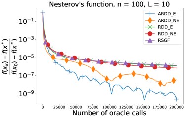
Refer to caption
Refer to caption
Refer to caption
Figure 1: ARDD, RDD and RSGF applied to minimize Nesterov’s function (62). We use _E and _NE to define 2subscript2\ell_{2} and 1subscript1\ell_{1} proximal setups respectively (see (8) and (9) for the details). In the plot for n=5000𝑛5000n=5000 number of oracle calls is divided by 107superscript10710^{7}.

In these settings x0x1=x0x2subscriptnormsubscript𝑥0superscript𝑥1subscriptnormsubscript𝑥0superscript𝑥2\|x_{0}-x^{*}\|_{1}=\|x_{0}-x^{*}\|_{2} and our theory establishes (see Tables 1 and 2) better complexity bounds for the case when p=1𝑝1p=1 then for the Euclidean case especially for big n𝑛n. The experiments confirm this claim: as one can see in Figure 1, the choice of 1subscript1\ell_{1} proximal setup becomes more beneficial than standard Euclidean setup for n=1000𝑛1000n=1000 and n=5000𝑛5000n=5000 to reach good enough accuracy. Indeed, our choice of the starting point and L𝐿L implies that f(x0)f(x)200𝑓subscript𝑥0𝑓superscript𝑥200f(x_{0})-f(x^{*})\approx 200 and for n=1000𝑛1000n=1000 and n=5000𝑛5000n=5000 ARDD with 1subscript1\ell_{1} proximal setup (ARDD_NE in Figure 1) make f(xN)f(x)𝑓subscript𝑥𝑁𝑓superscript𝑥f(x_{N})-f(x^{*}) of order 103105superscript103superscript10510^{-3}-10^{-5} faster than ARDD with p=2𝑝2p=2 (ARDD_E in Figure 1) and RDD with p=1𝑝1p=1 (RDD_NE in Figure 1) finds such xNsuperscript𝑥𝑁x^{N} that f(xN)f(x)𝑓superscript𝑥𝑁𝑓superscript𝑥f(x^{N})-f(x^{*}) is of order 103superscript10310^{-3} faster than its Euclidean counterpart (RDD_E in Figure 1). Finally, all of our methods outperform RSGF on the considered problem.

To perform mirror descent step for p=1𝑝1p=1 we apply relations obtained in Appendix B from [45]. See other details connected with parameters tuning in C of this work.

6.2 Least squares problem

In this subsection we consider least squares problem:

minxn{f(x)=12rAxb22=1ri=1r12(Aixbi)2}.subscript𝑥superscript𝑛𝑓𝑥12𝑟superscriptsubscriptnorm𝐴𝑥𝑏221𝑟superscriptsubscript𝑖1𝑟12superscriptsubscript𝐴𝑖𝑥subscript𝑏𝑖2\min\limits_{x\in\mathbb{R}^{n}}\left\{f(x)=\frac{1}{2r}\|Ax-b\|_{2}^{2}=\frac{1}{r}\sum\limits_{i=1}^{r}\frac{1}{2}(A_{i}x-b_{i})^{2}\right\}. (63)

Here A𝐴A is r×n𝑟𝑛r\times n real matrix, br𝑏superscript𝑟b\in\mathbb{R}^{r} and Aisubscript𝐴𝑖A_{i} denotes the i𝑖i-th row of A𝐴A. Clearly, f(x)𝑓𝑥f(x) is convex and smooth function. Moreover, each summand fi(x)=12(Aixbi)2subscript𝑓𝑖𝑥12superscriptsubscript𝐴𝑖𝑥subscript𝑏𝑖2f_{i}(x)=\frac{1}{2}(A_{i}x-b_{i})^{2} is also convex and L2.isubscript𝐿formulae-sequence2𝑖L_{2.i}-smooth function with L2,i=Ai22subscript𝐿2𝑖superscriptsubscriptnormsubscript𝐴𝑖22L_{2,i}=\|A_{i}\|_{2}^{2}. One can consider (63) as (1) with F(x,ξ)=fξ(x)=12(Aξxbξ)2𝐹𝑥𝜉subscript𝑓𝜉𝑥12superscriptsubscript𝐴𝜉𝑥subscript𝑏𝜉2F(x,\xi)=f_{\xi}(x)=\frac{1}{2}(A_{\xi}x-b_{\xi})^{2} where ξ𝜉\xi is uniformly distributed on {1,2,,r}12𝑟\{1,2,\ldots,r\}. Then, by definition of L2subscript𝐿2L_{2} we have

L2=𝔼ξL2,ξ2=1ri=1rAi22=AFrsubscript𝐿2subscript𝔼𝜉superscriptsubscript𝐿2𝜉21𝑟superscriptsubscript𝑖1𝑟superscriptsubscriptnormsubscript𝐴𝑖22subscriptnorm𝐴𝐹𝑟L_{2}=\sqrt{\mathbb{E}_{\xi}L_{2,\xi}^{2}}=\sqrt{\frac{1}{r}\sum\limits_{i=1}^{r}\|A_{i}\|_{2}^{2}}=\frac{\|A\|_{F}}{\sqrt{r}} (64)

where AFsubscriptnorm𝐴𝐹\|A\|_{F} denotes Frobenius norm of matrix A𝐴A.

In our preliminary experiments elements of A𝐴A and b𝑏b were sampled independently from the standard normal distribution and then matrix A𝐴A was normalized by its 2subscript2\ell_{2}-norm. In particular, we choose r=300𝑟300r=300 and n=400𝑛400n=400 which implies that f(x)𝑓𝑥f(x) is just convex but not strongly convex and f(x)=0𝑓superscript𝑥0f(x^{*})=0. Moreover, we compute the solution xsuperscript𝑥x^{*} as A+bsuperscript𝐴𝑏A^{+}b where A+superscript𝐴A^{+} denotes Moore-Penrose inverse of A𝐴A and choose the starting point x0subscript𝑥0x_{0} as xsuperscript𝑥x^{*} and 100100100 to the first component. In our tests the suboptimality of the starting point, i.e. f(x0)f(x)𝑓subscript𝑥0𝑓superscript𝑥f(x_{0})-f(x^{*}), was approximately 333. The results can be found in Figure 2.
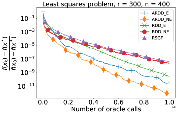
Refer to caption
Figure 2: ARDD, RDD and RSGF applied to solve least squares problem (63). We use _E and _NE to define 2subscript2\ell_{2} and 1subscript1\ell_{1} proximal setups respectively (see (8) and (9) for the details). For all methods batch size m𝑚m equals 505050. By oracle call we mean one computation of functional value of a summand. Number of oracle calls is divided by 108superscript10810^{8}.

We want to notice that in these preliminary experiments with stochasticity in functional values in experiments with ARDD it was needed to tune not only αk+1subscript𝛼𝑘1\alpha_{k+1} that appears in the mirror descent step, but also the stepsize for the gradient step, see the details in C.

7 Conclusion

In this paper we propose four novel directional derivative methods for smooth stochastic convex and strongly convex optimization with corollaries for derivative-free optimization. These methods are able to work with Euclidean and non-Euclidean proximal setups. We prove complexity results showing that in non-Euclidean case complexities of our methods outperform state-of-the-art results for directional derivative and derivative-free methods in terms of the dependence on the dimension of the problem under assumption that 1subscript1\ell_{1} and 2subscript2\ell_{2} norms of x0xsubscript𝑥0superscript𝑥x_{0}-x^{*} are close to each other, e.g. when x0=0subscript𝑥00x_{0}=0 and xsuperscript𝑥x^{*} is sparse. Moreover, we analyze our methods under general assumptions on the noisy oracle and provide bounds for the admissible noise levels. Since we use mini-batches, we are able to separate iteration complexity and sample complexity, the former being up to a dimension-dependent factor the same as for accelerated gradient method in the standard deterministic full-gradient setting. This makes our methods amenable to parallel computation setting [29] and leads to acceleration in this setting compared to standard stochastic gradient methods [26]. Finally, we conduct several experiments providing numerical justifications of the obtained results.

Using an additional “light-tail” assumption that 𝔼ξ[exp(g(x,ξ)f(x)22/σ2)]exp(1)subscript𝔼𝜉delimited-[]superscriptsubscriptnorm𝑔𝑥𝜉𝑓𝑥22superscript𝜎21\mathbb{E}_{\xi}[\exp(\|g(x,\xi)-\nabla f(x)\|_{2}^{2}/\sigma^{2})]\leqslant\exp(1) and techniques of [44] our algorithms and analysis can be extended to obtain results in terms of probability of large deviations. For example, in the case of controlled noise levels Δζ,ΔηsubscriptΔ𝜁subscriptΔ𝜂\Delta_{\zeta},\Delta_{\eta} this means that an algorithm outputs a point x^^𝑥\hat{x} which satisfies {f(x^)f(x)ε}1δ𝑓^𝑥𝑓superscript𝑥𝜀1𝛿\mathbb{P}\{f(\hat{x})-f(x^{*})\leqslant\varepsilon\}\geqslant 1-\delta, where δ(0,1)𝛿01\delta\in(0,1) is the confidence level, for the price of extra ln1δ1𝛿\ln\frac{1}{\delta} factor in N𝑁N and m𝑚m. As directions of future research we would like to point a primal-dual extension for problems with linear constraints in the spirit of [32, 22, 4, 7, 30, 27, 59], an extension with line-search to adapt to an unknown value of L2subscript𝐿2L_{2} using the techniques in [18, 12, 28], an extension for the case of intermediate smoothness [58, 48] or interpolation between accelerated and non-accelerated methods [36, 31], as well as extension to a more general type of inexactness called inexact model of the objective [69, 68].

Acknowledgements

The research is supported by the Ministry of Science and Higher Education of the Russian Federation (Goszadaniye) No. 075-00337-20-03, project No. 0714-2020-0005.

Appendix A Proof of Lemma 2.1

Here we prove that, for eRS2(1)𝑒𝑅subscript𝑆21e\in RS_{2}\left(1\right)

𝔼[eq2]min{q1, 16lnn8}n2q1,𝔼delimited-[]superscriptsubscriptnorm𝑒𝑞2𝑞116𝑛8superscript𝑛2𝑞1\mathbb{E}[\|e\|_{q}^{2}]\leqslant\min\{q-1,\,16\ln n-8\}n^{\frac{2}{q}-1}, (65)
𝔼[s,e2eq2]6s22min{q1,16lnn8}n2q2.𝔼delimited-[]superscript𝑠𝑒2superscriptsubscriptnorm𝑒𝑞26superscriptsubscriptnorm𝑠22𝑞116𝑛8superscript𝑛2𝑞2\mathbb{E}[\langle s,\,e\rangle^{2}\|e\|_{q}^{2}]\leqslant 6\|s\|_{2}^{2}\min\{q-1,16\ln n-8\}n^{\frac{2}{q}-2}. (66)

We start with proving the following inequality which could be rough for big q𝑞q:

𝔼[eq2](q1)n2q1,2q<.formulae-sequence𝔼delimited-[]superscriptsubscriptnorm𝑒𝑞2𝑞1superscript𝑛2𝑞12𝑞\mathbb{E}[\|e\|_{q}^{2}]\leqslant(q-1)n^{\frac{2}{q}-1},\quad 2\leqslant q<\infty. (67)

We have

𝔼[eq2]=𝔼[(k=1n|ek|q)2q](𝔼[k=1n|ek|q])2q=(n𝔼[|e2|q])2q,𝔼delimited-[]superscriptsubscriptnorm𝑒𝑞2𝔼delimited-[]superscriptsuperscriptsubscript𝑘1𝑛superscriptsubscript𝑒𝑘𝑞2𝑞superscript𝔼delimited-[]superscriptsubscript𝑘1𝑛superscriptsubscript𝑒𝑘𝑞2𝑞superscript𝑛𝔼delimited-[]superscriptsubscript𝑒2𝑞2𝑞missing-subexpression\begin{array}[]{rl}\mathbb{E}[\|e\|_{q}^{2}]=\mathbb{E}\left[\left(\sum\limits_{k=1}^{n}|e_{k}|^{q}\right)^{\frac{2}{q}}\right]\overset{\text{\char 172}}{\leqslant}\left(\mathbb{E}\left[\sum\limits_{k=1}^{n}|e_{k}|^{q}\right]\right)^{\frac{2}{q}}\overset{\text{\char 173}}{=}\left(n\mathbb{E}[|e_{2}|^{q}]\right)^{\frac{2}{q}},\end{array} (68)

where is due to probabilistic version of Jensen’s inequality (function φ(x)=x2q𝜑𝑥superscript𝑥2𝑞\varphi(x)=x^{\frac{2}{q}} is concave, because q2𝑞2q\geqslant 2) and is because mathematical expectation is linear and components of vector e𝑒e are identically distributed.

Moreover, due to Poincare lemma, we have

e=𝑑ξξ12++ξn2,𝑒𝑑𝜉superscriptsubscript𝜉12superscriptsubscript𝜉𝑛2e\overset{d}{=}\frac{\xi}{\sqrt{\xi_{1}^{2}+\dots+\xi_{n}^{2}}}, (69)

where ξ𝜉\xi is Gaussian random vector which mathematical expectation is zero vector and covariance matrix is identical. Then

𝔼[|e2|q]=𝔼[|ξ2|q(ξ12++ξn2)q2]=∫⋯∫n|x2|q(k=1nxk2)q21(2π)n2exp(12k=1nxk2)𝑑x1𝑑xn.𝔼delimited-[]superscriptsubscript𝑒2𝑞𝔼delimited-[]superscriptsubscript𝜉2𝑞superscriptsuperscriptsubscript𝜉12superscriptsubscript𝜉𝑛2𝑞2missing-subexpressionabsentsubscriptmultiple-integralsuperscript𝑛superscriptsubscript𝑥2𝑞superscriptsuperscriptsubscript𝑘1𝑛superscriptsubscript𝑥𝑘2𝑞21superscript2𝜋𝑛212superscriptsubscript𝑘1𝑛superscriptsubscript𝑥𝑘2differential-dsubscript𝑥1differential-dsubscript𝑥𝑛missing-subexpression\begin{array}[]{rl}\mathbb{E}[|e_{2}|^{q}]=\mathbb{E}\left[\frac{|\xi_{2}|^{q}}{\left(\xi_{1}^{2}+\ldots+\xi_{n}^{2}\right)^{\frac{q}{2}}}\right]\\ =\idotsint\limits_{\mathbb{R}^{n}}|x_{2}|^{q}\left(\sum\limits_{k=1}^{n}x_{k}^{2}\right)^{-\frac{q}{2}}\cdot\frac{1}{(2\pi)^{\frac{n}{2}}}\cdot\exp\left(-\frac{1}{2}\sum\limits_{k=1}^{n}x_{k}^{2}\right)dx_{1}\ldots dx_{n}.\end{array}

Consider spherical coordinates:

x1=rcosφsinθ1sinθn2,x2=rsinφsinθ1sinθn2,x3=rcosθ1sinθ2sinθn2,x4=rcosθ2sinθ3sinθn2,xn=rcosθn2,r>0,φ[0,2π),θi[0,π],i=1,n2¯.subscript𝑥1𝑟𝜑subscript𝜃1subscript𝜃𝑛2missing-subexpressionsubscript𝑥2𝑟𝜑subscript𝜃1subscript𝜃𝑛2missing-subexpressionsubscript𝑥3𝑟subscript𝜃1subscript𝜃2subscript𝜃𝑛2missing-subexpressionsubscript𝑥4𝑟subscript𝜃2subscript𝜃3subscript𝜃𝑛2missing-subexpressionmissing-subexpressionsubscript𝑥𝑛𝑟subscript𝜃𝑛2missing-subexpressionformulae-sequence𝑟0formulae-sequence𝜑02𝜋formulae-sequencesubscript𝜃𝑖0𝜋𝑖¯1𝑛2missing-subexpression\begin{array}[]{rl}x_{1}=r\cos\varphi\sin\theta_{1}\ldots\sin\theta_{n-2},\\ x_{2}=r\sin\varphi\sin\theta_{1}\ldots\sin\theta_{n-2},\\ x_{3}=r\cos\theta_{1}\sin\theta_{2}\ldots\sin\theta_{n-2},\\ x_{4}=r\cos\theta_{2}\sin\theta_{3}\ldots\sin\theta_{n-2},\\ \ldots\\ x_{n}=r\cos\theta_{n-2},\\ r>0,\,\varphi\in[0,2\pi),\,\theta_{i}\in[0,\pi],\,i=\overline{1,n-2}.\end{array}

The Jacobian of mapping is

det((x1,,xn)(r,φ,θ1,θ2,,θn2))=rn1sinθ1(sinθ2)2(sinθn2)n2.subscript𝑥1subscript𝑥𝑛𝑟𝜑subscript𝜃1subscript𝜃2subscript𝜃𝑛2superscript𝑟𝑛1subscript𝜃1superscriptsubscript𝜃22superscriptsubscript𝜃𝑛2𝑛2\det\left(\frac{\partial(x_{1},\ldots,x_{n})}{\partial(r,\varphi,\theta_{1},\theta_{2},\ldots,\theta_{n-2})}\right)=r^{n-1}\sin\theta_{1}(\sin\theta_{2})^{2}\ldots(\sin\theta_{n-2})^{n-2}.

Then mathematical expectation 𝔼[|e2|q]𝔼delimited-[]superscriptsubscript𝑒2𝑞\mathbb{E}[|e_{2}|^{q}] could be rewritten in the following form:

𝔼[|e2|q]=∫⋯∫r>0,φ[0,2π),θi[0,π],i=1,n2¯rn1|sinφ|q|sinθ1|q+1|sinθ2|q+2|sinθn2|q+n2er22(2π)n2drdθn2=1(2π)n2IrIφIθ1Iθ2Iθn2,𝔼delimited-[]superscriptsubscript𝑒2𝑞missing-subexpressionabsentsubscriptmultiple-integralformulae-sequence𝑟0𝜑02𝜋formulae-sequencesubscript𝜃𝑖0𝜋𝑖¯1𝑛2superscript𝑟𝑛1superscript𝜑𝑞superscriptsubscript𝜃1𝑞1superscriptsubscript𝜃2𝑞2superscriptsubscript𝜃𝑛2𝑞𝑛2missing-subexpressionabsentsuperscript𝑒superscript𝑟22superscript2𝜋𝑛2𝑑𝑟𝑑subscript𝜃𝑛2missing-subexpressionabsent1superscript2𝜋𝑛2subscript𝐼𝑟subscript𝐼𝜑subscript𝐼subscript𝜃1subscript𝐼subscript𝜃2subscript𝐼subscript𝜃𝑛2missing-subexpression\begin{array}[]{rl}\mathbb{E}[|e_{2}|^{q}]\\ =\idotsint\limits_{\begin{subarray}{c}r>0,\,\varphi\in[0,2\pi),\\ \theta_{i}\in[0,\pi],\,i=\overline{1,n-2}\end{subarray}}r^{n-1}|\sin\varphi|^{q}|\sin\theta_{1}|^{q+1}|\sin\theta_{2}|^{q+2}\ldots|\sin\theta_{n-2}|^{q+n-2}\\ \cdot\frac{e^{-\frac{r^{2}}{2}}}{(2\pi)^{\frac{n}{2}}}dr\ldots d\theta_{n-2}\\ =\frac{1}{(2\pi)^{\frac{n}{2}}}I_{r}\cdot I_{\varphi}\cdot I_{\theta_{1}}\cdot I_{\theta_{2}}\cdot\ldots\cdot I_{\theta_{n-2}},\end{array}

where

Ir=0+rn1er22𝑑r,Iφ=02π|sinφ|q𝑑φ=20π|sinφ|q𝑑φ,Iθi=0π|sinθi|q+i𝑑θi,i=1,n2¯.subscript𝐼𝑟superscriptsubscript0superscript𝑟𝑛1superscript𝑒superscript𝑟22differential-d𝑟missing-subexpressionsubscript𝐼𝜑superscriptsubscript02𝜋superscript𝜑𝑞differential-d𝜑2superscriptsubscript0𝜋superscript𝜑𝑞differential-d𝜑missing-subexpressionformulae-sequencesubscript𝐼subscript𝜃𝑖superscriptsubscript0𝜋superscriptsubscript𝜃𝑖𝑞𝑖differential-dsubscript𝜃𝑖𝑖¯1𝑛2missing-subexpression\begin{array}[]{rl}I_{r}=\int\limits_{0}^{+\infty}r^{n-1}e^{-\frac{r^{2}}{2}}dr,\\ I_{\varphi}=\int\limits_{0}^{2\pi}|\sin\varphi|^{q}d\varphi=2\int\limits_{0}^{\pi}|\sin\varphi|^{q}d\varphi,\\ I_{\theta_{i}}=\int\limits_{0}^{\pi}|\sin\theta_{i}|^{q+i}d\theta_{i},\,i=\overline{1,n-2}.\end{array}

Now we are going to compute these integrals. Start with Irsubscript𝐼𝑟I_{r}:

Ir=0+rn1er22dr=/r=2t/=0+(2t)n21etdt=2n21Γ(n2).\begin{array}[]{rl}I_{r}=\int\limits_{0}^{+\infty}r^{n-1}e^{-\frac{r^{2}}{2}}dr=/r=\sqrt{2t}/=\int\limits_{0}^{+\infty}(2t)^{\frac{n}{2}-1}e^{-t}dt=2^{\frac{n}{2}-1}\Gamma(\frac{n}{2}).\end{array}

To compute other integrals it is useful to consider the following integral (α>0)𝛼0(\alpha>0):

0π|sinφ|αdφ=20π2|sinφ|αdφ=20π2(sin2φ)α2dφ=/t=sin2φ/=01tα12(1t)12𝑑t=B(α+12,12)=Γ(α+12)Γ(12)Γ(α+22)=πΓ(α+12)Γ(α+22).\begin{array}[]{rl}\int\limits_{0}^{\pi}|\sin\varphi|^{\alpha}d\varphi=2\int\limits_{0}^{\frac{\pi}{2}}|\sin\varphi|^{\alpha}d\varphi=2\int\limits_{0}^{\frac{\pi}{2}}(\sin^{2}\varphi)^{\frac{\alpha}{2}}d\varphi=/t=\sin^{2}\varphi/\\ =\int\limits_{0}^{1}t^{\frac{\alpha-1}{2}}(1-t)^{-\frac{1}{2}}dt=B(\frac{\alpha+1}{2},\,\frac{1}{2})=\frac{\Gamma(\frac{\alpha+1}{2})\Gamma(\frac{1}{2})}{\Gamma(\frac{\alpha+2}{2})}=\sqrt{\pi}\frac{\Gamma(\frac{\alpha+1}{2})}{\Gamma(\frac{\alpha+2}{2})}.\end{array}

From this we obtain

𝔼[|e2|q]=1(2π)n2IrIφIθ1Iθ2Iθn2=1(2π)n22n21Γ(n2)2πΓ(q+12)Γ(q+22)πΓ(q+22)Γ(q+32)πΓ(q+32)Γ(q+42)πΓ(q+n12)Γ(q+n2)=1πΓ(n2)Γ(q+12)Γ(q+n2).𝔼delimited-[]superscriptsubscript𝑒2𝑞1superscript2𝜋𝑛2subscript𝐼𝑟subscript𝐼𝜑subscript𝐼subscript𝜃1subscript𝐼subscript𝜃2subscript𝐼subscript𝜃𝑛2missing-subexpressionabsent1superscript2𝜋𝑛2superscript2𝑛21Γ𝑛22𝜋Γ𝑞12Γ𝑞22𝜋Γ𝑞22Γ𝑞32𝜋Γ𝑞32Γ𝑞42𝜋Γ𝑞𝑛12Γ𝑞𝑛2missing-subexpressionabsent1𝜋Γ𝑛2Γ𝑞12Γ𝑞𝑛2missing-subexpression\begin{array}[]{rl}\mathbb{E}[|e_{2}|^{q}]=\frac{1}{(2\pi)^{\frac{n}{2}}}I_{r}\cdot I_{\varphi}\cdot I_{\theta_{1}}\cdot I_{\theta_{2}}\cdot\ldots\cdot I_{\theta_{n-2}}\\ =\frac{1}{(2\pi)^{\frac{n}{2}}}\cdot 2^{\frac{n}{2}-1}\Gamma(\frac{n}{2})\cdot 2\sqrt{\pi}\frac{\Gamma(\frac{q+1}{2})}{\Gamma(\frac{q+2}{2})}\cdot\sqrt{\pi}\frac{\Gamma(\frac{q+2}{2})}{\Gamma(\frac{q+3}{2})}\cdot\sqrt{\pi}\frac{\Gamma(\frac{q+3}{2})}{\Gamma(\frac{q+4}{2})}\cdot\ldots\cdot\sqrt{\pi}\frac{\Gamma(\frac{q+n-1}{2})}{\Gamma(\frac{q+n}{2})}\\ =\frac{1}{\sqrt{\pi}}\cdot\frac{\Gamma(\frac{n}{2})\Gamma(\frac{q+1}{2})}{\Gamma(\frac{q+n}{2})}.\end{array} (70)

Now, we want to show that q2for-all𝑞2\forall\,q\geqslant 2

1πΓ(n2)Γ(q+12)Γ(q+n2)(q1n)q2.1𝜋Γ𝑛2Γ𝑞12Γ𝑞𝑛2superscript𝑞1𝑛𝑞2\frac{1}{\sqrt{\pi}}\cdot\frac{\Gamma(\frac{n}{2})\Gamma(\frac{q+1}{2})}{\Gamma(\frac{q+n}{2})}\leqslant\left(\frac{q-1}{n}\right)^{\frac{q}{2}}. (71)

At the beginning show that (71) holds for q=2𝑞2q=2 (and arbitrary n𝑛n):

1πΓ(n2)Γ(2+12)Γ(2+n2)1n=1πΓ(n2)12Γ(12)n2Γ(n2)1n=1n1n=00.1𝜋Γ𝑛2Γ212Γ2𝑛21𝑛1𝜋Γ𝑛212Γ12𝑛2Γ𝑛21𝑛1𝑛1𝑛00\frac{1}{\sqrt{\pi}}\cdot\frac{\Gamma(\frac{n}{2})\Gamma(\frac{2+1}{2})}{\Gamma(\frac{2+n}{2})}-\frac{1}{n}=\frac{1}{\sqrt{\pi}}\cdot\frac{\Gamma(\frac{n}{2})\cdot\frac{1}{2}\Gamma(\frac{1}{2})}{\frac{n}{2}\Gamma(\frac{n}{2})}-\frac{1}{n}=\frac{1}{n}-\frac{1}{n}=0\leqslant 0.

Consider the function

fn(q)=1πΓ(n2)Γ(q+12)Γ(q+n2)(q1n)q2subscript𝑓𝑛𝑞1𝜋Γ𝑛2Γ𝑞12Γ𝑞𝑛2superscript𝑞1𝑛𝑞2f_{n}(q)=\frac{1}{\sqrt{\pi}}\cdot\frac{\Gamma(\frac{n}{2})\Gamma(\frac{q+1}{2})}{\Gamma(\frac{q+n}{2})}-\left(\frac{q-1}{n}\right)^{\frac{q}{2}}

where q2𝑞2q\geqslant 2. Also consider ψ(x)=d(ln(Γ(x)))dx𝜓𝑥𝑑Γ𝑥𝑑𝑥\psi(x)=\frac{d(\ln(\Gamma(x)))}{dx} with x>0𝑥0x>0 which is called (digamma function). For gamma function it holds

Γ(x+1)=xΓ(x),x>0.formulae-sequenceΓ𝑥1𝑥Γ𝑥𝑥0\Gamma(x+1)=x\Gamma(x),\,x>0.

Taking natural logarithm from it and taking derivative w.r.t. x𝑥x:

lnΓ(x+1)=lnΓ(x)+lnx,d(ln(Γ(x+1)))dx=d(ln(Γ(x)))dx+1x,Γ𝑥1Γ𝑥𝑥missing-subexpression𝑑Γ𝑥1𝑑𝑥𝑑Γ𝑥𝑑𝑥1𝑥missing-subexpression\begin{array}[]{rl}\ln\Gamma(x+1)=\ln\Gamma(x)+\ln x,\\ \frac{d(\ln(\Gamma(x+1)))}{dx}=\frac{d(\ln(\Gamma(x)))}{dx}+\frac{1}{x},\end{array}

which could be written in digamma-function-notation:

ψ(x+1)=ψ(x)+1x.𝜓𝑥1𝜓𝑥1𝑥\psi(x+1)=\psi(x)+\frac{1}{x}. (72)

One can show that digamma function is monotonically increases when x>0𝑥0x>0. To prove this fact we are going to show that

(Γ(x))2<Γ(x)Γ′′(x).superscriptsuperscriptΓ𝑥2Γ𝑥superscriptΓ′′𝑥\left(\Gamma^{\prime}(x)\right)^{2}<\Gamma(x)\Gamma^{\prime\prime}(x). (73)

That is,

(Γ(x))2=(0+etlnttx1dt)2<0+(et2tx12)2𝑑t0+(et2tx12lnt)2𝑑t=0+ettx1𝑑tΓ(x)0+ettx1ln2tdtΓ′′(x),superscriptsuperscriptΓ𝑥2superscriptsuperscriptsubscript0superscript𝑒𝑡𝑡superscript𝑡𝑥1𝑑𝑡2missing-subexpressionsuperscriptsubscript0superscriptsuperscript𝑒𝑡2superscript𝑡𝑥122differential-d𝑡superscriptsubscript0superscriptsuperscript𝑒𝑡2superscript𝑡𝑥12𝑡2differential-d𝑡subscriptsuperscriptsubscript0superscript𝑒𝑡superscript𝑡𝑥1differential-d𝑡Γ𝑥subscriptsuperscriptsubscript0superscript𝑒𝑡superscript𝑡𝑥1superscript2𝑡𝑑𝑡superscriptΓ′′𝑥missing-subexpression\begin{array}[]{rl}\left(\Gamma^{\prime}(x)\right)^{2}=\left(\int\limits_{0}^{+\infty}e^{-t}\ln t\cdot t^{x-1}dt\right)^{2}\\ \overset{\text{\char 172}}{<}\int\limits_{0}^{+\infty}\left(e^{-\frac{t}{2}}t^{\frac{x-1}{2}}\right)^{2}dt\cdot\int\limits_{0}^{+\infty}\left(e^{-\frac{t}{2}}t^{\frac{x-1}{2}}\ln t\right)^{2}dt=\underbrace{\int\limits_{0}^{+\infty}e^{-t}t^{x-1}dt}_{\Gamma(x)}\cdot\underbrace{\int\limits_{0}^{+\infty}e^{t}t^{x-1}\ln^{2}tdt}_{\Gamma^{\prime\prime}(x)},\end{array}

where follows from Cauchy-Schwartz inequality (the equality cannot occur because functions et2tx12superscript𝑒𝑡2superscript𝑡𝑥12e^{-\frac{t}{2}}t^{\frac{x-1}{2}} and et2tx12lntsuperscript𝑒𝑡2superscript𝑡𝑥12𝑡e^{-\frac{t}{2}}t^{\frac{x-1}{2}}\ln t are linearly independent). From (73) follows that

d2(lnΓ(x))dx2=(Γ(x)Γ(x))=Γ′′(x)Γ(x)(Γ(x))2(Γ(x))2>(73)0,superscript𝑑2Γ𝑥𝑑superscript𝑥2superscriptsuperscriptΓ𝑥Γ𝑥superscriptΓ′′𝑥Γ𝑥superscriptsuperscriptΓ𝑥2superscriptΓ𝑥2italic-(73italic-)0\frac{d^{2}(\ln\Gamma(x))}{dx^{2}}=\left(\frac{\Gamma^{\prime}(x)}{\Gamma(x)}\right)^{\prime}=\frac{\Gamma^{\prime\prime}(x)}{\Gamma(x)}-\frac{\left(\Gamma^{\prime}(x)\right)^{2}}{\left(\Gamma(x)\right)^{2}}\overset{\eqref{lemm1:digamma_decrease}}{>}0,

which shows that digamma function increases.

Now we show that fn(q)subscript𝑓𝑛𝑞f_{n}(q) decreases on the interval [2,+)2[2,+\infty). To obtain it is sufficient to consider ln(f(q))𝑓𝑞\ln(f(q)):

ln(fn(q))=ln(Γ(n2)π)+ln(Γ(q+12))ln(Γ(q+n2))q2(ln(q1)lnn),d(ln(fn(q)))dq=12ψ(q+12)12ψ(q+n2)12ln(q1)q2(q1)+12lnn.subscript𝑓𝑛𝑞missing-subexpressionabsentΓ𝑛2𝜋Γ𝑞12Γ𝑞𝑛2𝑞2𝑞1𝑛missing-subexpression𝑑subscript𝑓𝑛𝑞𝑑𝑞12𝜓𝑞1212𝜓𝑞𝑛212𝑞1𝑞2𝑞112𝑛missing-subexpression\begin{array}[]{rl}\ln(f_{n}(q))\\ =\ln\left(\frac{\Gamma(\frac{n}{2})}{\sqrt{\pi}}\right)+\ln\left(\Gamma\left(\frac{q+1}{2}\right)\right)-\ln\left(\Gamma\left(\frac{q+n}{2}\right)\right)-\frac{q}{2}\left(\ln(q-1)-\ln n\right),\\ \frac{d(\ln(f_{n}(q)))}{dq}=\frac{1}{2}\psi\left(\frac{q+1}{2}\right)-\frac{1}{2}\psi\left(\frac{q+n}{2}\right)-\frac{1}{2}\ln(q-1)-\frac{q}{2(q-1)}+\frac{1}{2}\ln n.\end{array}

We are going to show that d(ln(fn(q)))dq<0𝑑subscript𝑓𝑛𝑞𝑑𝑞0\frac{d(\ln(f_{n}(q)))}{dq}<0 for q2𝑞2q\geqslant 2. Let k=n2𝑘𝑛2k=\lfloor\frac{n}{2}\rfloor (the closest integer which is no greater than n2𝑛2\frac{n}{2}). Then ψ(q+n2)>ψ(k1+q+12)𝜓𝑞𝑛2𝜓𝑘1𝑞12\psi\left(\frac{q+n}{2}\right)>\psi\left(k-1+\frac{q+1}{2}\right) and lnnln(2k+1)𝑛2𝑘1\ln n\leqslant\ln(2k+1), whence

d(ln(fn(q)))dq<12(ψ(q+12)ψ(k1+q+12))12ln(q1)q2(q1)+12ln(2k+1)=(72)12(ψ(q+12)i=1k11q+12+ki1ψ(q+12))q2(q1)+12ln(2k+1q1)12i=1k12q1+2k2i1q1+12ln(2k+1q1)=12(2q1+2q+1+2q+3++2q+2k3)+12ln(2k+1q1)<12ln(q+2k1q1)+12ln(2k+1q1)12ln(2k+1q1)+12ln(2k+1q1)=0,𝑑subscript𝑓𝑛𝑞𝑑𝑞missing-subexpressionabsent12𝜓𝑞12𝜓𝑘1𝑞1212𝑞1𝑞2𝑞1122𝑘1missing-subexpressionitalic-(72italic-)12𝜓𝑞12superscriptsubscript𝑖1𝑘11𝑞12𝑘𝑖1𝜓𝑞12𝑞2𝑞1122𝑘1𝑞1missing-subexpression12superscriptsubscript𝑖1𝑘12𝑞12𝑘2𝑖1𝑞1122𝑘1𝑞1missing-subexpressionabsent122𝑞12𝑞12𝑞32𝑞2𝑘3122𝑘1𝑞1missing-subexpression12𝑞2𝑘1𝑞1122𝑘1𝑞1122𝑘1𝑞1122𝑘1𝑞10missing-subexpression\begin{array}[]{rl}\frac{d(\ln(f_{n}(q)))}{dq}\\ <\frac{1}{2}\left(\psi\left(\frac{q+1}{2}\right)-\psi\left(k-1+\frac{q+1}{2}\right)\right)-\frac{1}{2}\ln(q-1)-\frac{q}{2(q-1)}+\frac{1}{2}\ln(2k+1)\\ \overset{\eqref{lemm1:digamma_recurrence}}{=}\frac{1}{2}\left(\psi\left(\frac{q+1}{2}\right)-\sum\limits_{i=1}^{k-1}\frac{1}{\frac{q+1}{2}+k-i-1}-\psi\left(\frac{q+1}{2}\right)\right)-\frac{q}{2(q-1)}+\frac{1}{2}\ln\left(\frac{2k+1}{q-1}\right)\\ \overset{\text{\char 172}}{\leqslant}-\frac{1}{2}\sum\limits_{i=1}^{k-1}\frac{2}{q-1+2k-2i}-\frac{1}{q-1}+\frac{1}{2}\ln\left(\frac{2k+1}{q-1}\right)\\ =-\frac{1}{2}\left(\frac{2}{q-1}+\frac{2}{q+1}+\frac{2}{q+3}+\ldots+\frac{2}{q+2k-3}\right)+\frac{1}{2}\ln\left(\frac{2k+1}{q-1}\right)\\ \overset{\text{\char 173}}{<}-\frac{1}{2}\ln\left(\frac{q+2k-1}{q-1}\right)+\frac{1}{2}\ln\left(\frac{2k+1}{q-1}\right)\overset{\text{\char 174}}{\leqslant}-\frac{1}{2}\ln\left(\frac{2k+1}{q-1}\right)+\frac{1}{2}\ln\left(\frac{2k+1}{q-1}\right)=0,\end{array}

where and is because q2𝑞2q\geqslant 2, is due to estimation of integral of 1x1𝑥\frac{1}{x} by integral of g(x)=1q1+2i,x[q1+2i,q1+2i+2],i=0,2k1¯formulae-sequence𝑔𝑥1𝑞12𝑖formulae-sequence𝑥𝑞12𝑖𝑞12𝑖2𝑖¯02𝑘1g(x)=\frac{1}{q-1+2i},\,x\in[q-1+2i,q-1+2i+2],\,i=\overline{0,2k-1} which is no less than f(x)𝑓𝑥f(x):

2q1+2q+1+2q+3++2q+2k3>q1q+2k11x𝑑x=ln(q+2k1q1).2𝑞12𝑞12𝑞32𝑞2𝑘3superscriptsubscript𝑞1𝑞2𝑘11𝑥differential-d𝑥𝑞2𝑘1𝑞1\frac{2}{q-1}+\frac{2}{q+1}+\frac{2}{q+3}+\ldots+\frac{2}{q+2k-3}>\int\limits_{q-1}^{q+2k-1}\frac{1}{x}dx=\ln\left(\frac{q+2k-1}{q-1}\right).

So, we shown that d(ln(fn(q)))dq<0𝑑subscript𝑓𝑛𝑞𝑑𝑞0\frac{d(\ln(f_{n}(q)))}{dq}<0 for q2𝑞2q\geqslant 2 arbitrary natural number n𝑛n. Therefore for any fixed number n𝑛n the function fn(q)subscript𝑓𝑛𝑞f_{n}(q) decreases as q𝑞q increase, which means that fn(q)fn(2)=0subscript𝑓𝑛𝑞subscript𝑓𝑛20f_{n}(q)\leqslant f_{n}(2)=0, i.e., (71) holds. From this and (68),(70) we obtain that q2for-all𝑞2\forall\,q\geqslant 2

𝔼[eq2](68)(n𝔼[|e2|q])2q(70),(71)(q1)n2q1.𝔼delimited-[]superscriptsubscriptnorm𝑒𝑞2italic-(68italic-)superscript𝑛𝔼delimited-[]superscriptsubscript𝑒2𝑞2𝑞italic-(70italic-)italic-(71italic-)𝑞1superscript𝑛2𝑞1\mathbb{E}[||e||_{q}^{2}]\overset{\eqref{lemm1:jensen}}{\leqslant}\left(n\mathbb{E}[|e_{2}|^{q}]\right)^{\frac{2}{q}}\overset{\eqref{lemm1:expectation_component},\eqref{lemm1:key_estimation}}{\leqslant}(q-1)n^{\frac{2}{q}-1}. (74)

However, inequality (74) is useless when q𝑞q is big (with respect to n𝑛n). Consider left hand side of (74) as function of q𝑞q and find its minimum for q2𝑞2q\geqslant 2. Consider hn(q)=ln(q1)+(2q1)lnnsubscript𝑛𝑞𝑞12𝑞1𝑛h_{n}(q)=\ln(q-1)+\left(\frac{2}{q}-1\right)\ln n (it is logarithm of the right hand side of (74)). Derivative of h(q)𝑞h(q) is

dh(q)dq=1q12lnnq2,1q12lnnq2=0,q22qlnn+2lnn=0.𝑑𝑞𝑑𝑞1𝑞12𝑛superscript𝑞2missing-subexpression1𝑞12𝑛superscript𝑞20missing-subexpressionsuperscript𝑞22𝑞𝑛2𝑛0missing-subexpression\begin{array}[]{rl}\frac{dh(q)}{dq}=\frac{1}{q-1}-\frac{2\ln n}{q^{2}},\\ \frac{1}{q-1}-\frac{2\ln n}{q^{2}}=0,\\ q^{2}-2q\ln n+2\ln n=0.\end{array}

If n8𝑛8n\geqslant 8, then the point where the function obtains its minimum on the set [2,+)2[2,+\infty) is q0=lnn(1+12lnn)subscript𝑞0𝑛112𝑛q_{0}=\ln n\left(1+\sqrt{1-\frac{2}{\ln n}}\right) (for the case n7𝑛7n\leqslant 7 it turns out that q0=2subscript𝑞02q_{0}=2; further without loss of generality we assume n8𝑛8n\geqslant 8). Therefore for all q>q0𝑞subscript𝑞0q>q_{0} it is more useful to use the following estimation:

𝔼[eq2]<𝔼[eq02](74)(q01)n2q01(2lnn1)n2lnn1=(2lnn1)e21n(16lnn8)1n(16lnn8)n2q1,𝔼delimited-[]superscriptsubscriptnorm𝑒𝑞2𝔼delimited-[]superscriptsubscriptnorm𝑒subscript𝑞02italic-(74italic-)subscript𝑞01superscript𝑛2subscript𝑞012𝑛1superscript𝑛2𝑛1missing-subexpressionabsent2𝑛1superscript𝑒21𝑛16𝑛81𝑛16𝑛8superscript𝑛2𝑞1missing-subexpression\begin{array}[]{rl}\mathbb{E}[||e||_{q}^{2}]\overset{\text{\char 172}}{<}\mathbb{E}[||e||_{q_{0}}^{2}]\overset{\eqref{lemm1:pre-final}}{\leqslant}(q_{0}-1)n^{\frac{2}{q_{0}}-1}\overset{\text{\char 173}}{\leqslant}(2\ln n-1)n^{\frac{2}{\ln n}-1}\\ =(2\ln n-1)e^{2}\frac{1}{n}\leqslant(16\ln n-8)\frac{1}{n}\leqslant(16\ln n-8)n^{\frac{2}{q}-1},\end{array} (75)

where is due to eq<eq0subscriptnorm𝑒𝑞subscriptnorm𝑒subscript𝑞0\|e\|_{q}<\|e\|_{q_{0}} for q>q0𝑞subscript𝑞0q>q_{0}, follows from q02lnn,q0lnnformulae-sequencesubscript𝑞02𝑛subscript𝑞0𝑛q_{0}\leqslant 2\ln n,\,q_{0}\geqslant\ln n. Putting estimations (74) and (75) together we obtain (65).

Now we are going to prove (66). Firstly, we want to estimate 𝔼[eq4]𝔼delimited-[]superscriptsubscriptnorm𝑒𝑞4\sqrt{\mathbb{E}[\|e\|_{q}^{4}]}. Due to probabilistic Jensen’s inequality (q2𝑞2q\geqslant 2)

𝔼[eq4]=𝔼[((k=1n|ek|q)2)2q](𝔼[(k=1n|ek|q)2])2q(𝔼[(nk=1n|ek|2q)])2q=(n2𝔼[|e2|2q])2q(70),(71)n4q((2q1n)2q2)2q=(2q1)2n4q2,𝔼delimited-[]superscriptsubscriptnorm𝑒𝑞4𝔼delimited-[]superscriptsuperscriptsuperscriptsubscript𝑘1𝑛superscriptsubscript𝑒𝑘𝑞22𝑞superscript𝔼delimited-[]superscriptsuperscriptsubscript𝑘1𝑛superscriptsubscript𝑒𝑘𝑞22𝑞missing-subexpressionsuperscript𝔼delimited-[]𝑛superscriptsubscript𝑘1𝑛superscriptsubscript𝑒𝑘2𝑞2𝑞superscriptsuperscript𝑛2𝔼delimited-[]superscriptsubscript𝑒22𝑞2𝑞missing-subexpressionitalic-(70italic-)italic-(71italic-)superscript𝑛4𝑞superscriptsuperscript2𝑞1𝑛2𝑞22𝑞superscript2𝑞12superscript𝑛4𝑞2missing-subexpression\begin{array}[]{rl}\mathbb{E}[||e||_{q}^{4}]=\mathbb{E}\left[\left(\left(\sum\limits_{k=1}^{n}|e_{k}|^{q}\right)^{2}\right)^{\frac{2}{q}}\right]\leqslant\left(\mathbb{E}\left[\left(\sum\limits_{k=1}^{n}|e_{k}|^{q}\right)^{2}\right]\right)^{\frac{2}{q}}\\ \overset{\text{\char 172}}{\leqslant}\left(\mathbb{E}\left[\left(n\sum\limits_{k=1}^{n}|e_{k}|^{2q}\right)\right]\right)^{\frac{2}{q}}\overset{\text{\char 173}}{=}\left(n^{2}\mathbb{E}[|e_{2}|^{2q}]\right)^{\frac{2}{q}}\\ \overset{\eqref{lemm1:expectation_component},\eqref{lemm1:key_estimation}}{\leqslant}n^{\frac{4}{q}}\left(\left(\frac{2q-1}{n}\right)^{\frac{2q}{2}}\right)^{\frac{2}{q}}=(2q-1)^{2}n^{\frac{4}{q}-2},\end{array}

where is because (k=1nxk)2nk=1nxk2superscriptsuperscriptsubscript𝑘1𝑛subscript𝑥𝑘2𝑛superscriptsubscript𝑘1𝑛superscriptsubscript𝑥𝑘2\left(\sum\limits_{k=1}^{n}x_{k}\right)^{2}\leqslant n\sum\limits_{k=1}^{n}x_{k}^{2} for x1,x2,,xnsubscript𝑥1subscript𝑥2subscript𝑥𝑛x_{1},x_{2},\ldots,x_{n}\in\mathbb{R} and follows from that mathematical expectation is linear and components of the random vector e𝑒e are identically distributed. From this we obtain

𝔼[eq4](2q1)n2q1.𝔼delimited-[]superscriptsubscriptnorm𝑒𝑞42𝑞1superscript𝑛2𝑞1\sqrt{\mathbb{E}[||e||_{q}^{4}]}\leqslant(2q-1)n^{\frac{2}{q}-1}. (76)

Consider the right hand side of the inequality (76) as a function of q𝑞q and find its minimum for q2𝑞2q\geqslant 2. Consider hn(q)=ln(2q1)+(2q1)lnnsubscript𝑛𝑞2𝑞12𝑞1𝑛h_{n}(q)=\ln(2q-1)+\left(\frac{2}{q}-1\right)\ln n (logarithm of the right hand side (76)). Derivative of h(q)𝑞h(q) is

dh(q)dq=22q12lnnq2,22q12lnnq2=0,q22qlnn+lnn=0.𝑑𝑞𝑑𝑞22𝑞12𝑛superscript𝑞2missing-subexpression22𝑞12𝑛superscript𝑞20missing-subexpressionsuperscript𝑞22𝑞𝑛𝑛0missing-subexpression\begin{array}[]{rl}\frac{dh(q)}{dq}=\frac{2}{2q-1}-\frac{2\ln n}{q^{2}},\\ \frac{2}{2q-1}-\frac{2\ln n}{q^{2}}=0,\\ q^{2}-2q\ln n+\ln n=0.\end{array}

If n3𝑛3n\geqslant 3, the the point where the function obtains its minimum on the set [2,+)2[2,+\infty) is q0=lnn(1+11lnn)subscript𝑞0𝑛111𝑛q_{0}=\ln n\left(1+\sqrt{1-\frac{1}{\ln n}}\right) (for the case n2𝑛2n\leqslant 2 it turns out that q0=2subscript𝑞02q_{0}=2; further without loss of generality we assume that n3𝑛3n\geqslant 3). Therefore for all q>q0𝑞subscript𝑞0q>q_{0}:

𝔼[eq4]<𝔼[eq04](76)(2q01)n2q01(4lnn1)n2lnn1=(4lnn1)e21n(32lnn8)1n(32lnn8)n2q1,𝔼delimited-[]superscriptsubscriptnorm𝑒𝑞4𝔼delimited-[]superscriptsubscriptnorm𝑒subscript𝑞04italic-(76italic-)2subscript𝑞01superscript𝑛2subscript𝑞014𝑛1superscript𝑛2𝑛1missing-subexpressionabsent4𝑛1superscript𝑒21𝑛32𝑛81𝑛32𝑛8superscript𝑛2𝑞1missing-subexpression\begin{array}[]{rl}\sqrt{\mathbb{E}[||e||_{q}^{4}]}\overset{\text{\char 172}}{<}\sqrt{\mathbb{E}[||e||_{q_{0}}^{4}]}\overset{\eqref{lemm1:pre_final_q_norm_power4}}{\leqslant}(2q_{0}-1)n^{\frac{2}{q_{0}}-1}\overset{\text{\char 173}}{\leqslant}(4\ln n-1)n^{\frac{2}{\ln n}-1}\\ =(4\ln n-1)e^{2}\frac{1}{n}\leqslant(32\ln n-8)\frac{1}{n}\leqslant(32\ln n-8)n^{\frac{2}{q}-1},\end{array} (77)

where is due to eq<eq0subscriptnorm𝑒𝑞subscriptnorm𝑒subscript𝑞0\|e\|_{q}<\|e\|_{q_{0}} for q>q0𝑞subscript𝑞0q>q_{0}, follows from q02lnn,q0lnnformulae-sequencesubscript𝑞02𝑛subscript𝑞0𝑛q_{0}\leqslant 2\ln n,\,q_{0}\geqslant\ln n. Putting estimations (76) and (77) together we get inequality

𝔼[eq4]min{2q1,32lnn8}n2q1.𝔼delimited-[]superscriptsubscriptnorm𝑒𝑞42𝑞132𝑛8superscript𝑛2𝑞1\sqrt{\mathbb{E}[||e||_{q}^{4}]}\leqslant\min\{2q-1,32\ln n-8\}n^{\frac{2}{q}-1}. (78)

Now we are going to find 𝔼[s,e4]𝔼delimited-[]superscript𝑠𝑒4\mathbb{E}[\langle s,\,e\rangle^{4}], where sn𝑠superscript𝑛s\in\mathbb{R}^{n} is some vector. Let Sn(r)subscript𝑆𝑛𝑟S_{n}(r) be a surface area of n𝑛n-dimensional Euclidean sphere with radius r𝑟r and dσ(e)𝑑𝜎𝑒d\sigma(e) be unnormalized uniform measure on n𝑛n-dimensional Euclidean sphere. From this it follows that Sn(r)=Sn(1)rn1,Sn1(1)Sn(1)=n1nπΓ(n+22)Γ(n+12)formulae-sequencesubscript𝑆𝑛𝑟subscript𝑆𝑛1superscript𝑟𝑛1subscript𝑆𝑛11subscript𝑆𝑛1𝑛1𝑛𝜋Γ𝑛22Γ𝑛12S_{n}(r)=S_{n}(1)r^{n-1},\,\frac{S_{n-1}(1)}{S_{n}(1)}=\frac{n-1}{n\sqrt{\pi}}\frac{\Gamma(\frac{n+2}{2})}{\Gamma(\frac{n+1}{2})}. Besides, let φ𝜑\varphi be the angle between s𝑠s and e𝑒e. Then

𝔼[s,e4]=1Sn(1)Ss,e4𝑑σ(φ)=1Sn(1)0πs24cos3φSn1(sinφ)𝑑φ=s24Sn1(1)Sn(1)0πcos4φsinn2φdφ=s24n1nπΓ(n+22)Γ(n+12)0πcos4φsinn2φdφ.𝔼delimited-[]superscript𝑠𝑒41subscript𝑆𝑛1subscript𝑆superscript𝑠𝑒4differential-d𝜎𝜑1subscript𝑆𝑛1superscriptsubscript0𝜋superscriptsubscriptnorm𝑠24superscript3𝜑subscript𝑆𝑛1𝜑differential-d𝜑missing-subexpressionabsentsuperscriptsubscriptnorm𝑠24subscript𝑆𝑛11subscript𝑆𝑛1superscriptsubscript0𝜋superscript4𝜑superscript𝑛2𝜑𝑑𝜑superscriptsubscriptnorm𝑠24𝑛1𝑛𝜋Γ𝑛22Γ𝑛12superscriptsubscript0𝜋superscript4𝜑superscript𝑛2𝜑𝑑𝜑missing-subexpression\begin{array}[]{rl}\mathbb{E}[\langle s,\,e\rangle^{4}]=\frac{1}{S_{n}(1)}\int\limits_{S}\langle s,\,e\rangle^{4}d\sigma(\varphi)=\frac{1}{S_{n}(1)}\int\limits_{0}^{\pi}||s||_{2}^{4}\cos^{3}\varphi S_{n-1}(\sin\varphi)d\varphi\\ =||s||_{2}^{4}\frac{S_{n-1}(1)}{S_{n}(1)}\int\limits_{0}^{\pi}\cos^{4}\varphi\sin^{n-2}\varphi d\varphi=||s||_{2}^{4}\cdot\frac{n-1}{n\sqrt{\pi}}\frac{\Gamma(\frac{n+2}{2})}{\Gamma(\frac{n+1}{2})}\int\limits_{0}^{\pi}\cos^{4}\varphi\sin^{n-2}\varphi d\varphi.\end{array} (79)

Compute the integral:

0πcos4φsinn2φdφ=20π2cos4φsinn2φdφ=/t=sin2φ/=0π2tn32(1t)32𝑑t=B(n12,52)=Γ(52)Γ(n12)Γ(n+42)=3212Γ(12)Γ(n12)n+22Γ(n+22)=3n+2πΓ(n12)2Γ(n+22).\begin{array}[]{rl}\int\limits_{0}^{\pi}\cos^{4}\varphi\sin^{n-2}\varphi d\varphi=2\int\limits_{0}^{\frac{\pi}{2}}\cos^{4}\varphi\sin^{n-2}\varphi d\varphi=/t=\sin^{2}\varphi/\\ =\int\limits_{0}^{\frac{\pi}{2}}t^{\frac{n-3}{2}}(1-t)^{\frac{3}{2}}dt=B(\frac{n-1}{2},\frac{5}{2})=\frac{\Gamma(\frac{5}{2})\Gamma(\frac{n-1}{2})}{\Gamma(\frac{n+4}{2})}=\frac{\frac{3}{2}\cdot\frac{1}{2}\Gamma(\frac{1}{2})\Gamma(\frac{n-1}{2})}{\frac{n+2}{2}\cdot\Gamma(\frac{n+2}{2})}=\frac{3}{n+2}\cdot\frac{\sqrt{\pi}\Gamma(\frac{n-1}{2})}{2\Gamma(\frac{n+2}{2})}.\end{array}

From this and (79) we obtain

𝔼[s,e4]=s24n1nπΓ(n+22)Γ(n+12)3n+2πΓ(n12)2Γ(n+22)=s243(n1)2n(n+2)Γ(n12)n12Γ(n12)=3s24n(n+2)3s24n2.𝔼delimited-[]superscript𝑠𝑒4superscriptsubscriptnorm𝑠24𝑛1𝑛𝜋Γ𝑛22Γ𝑛123𝑛2𝜋Γ𝑛122Γ𝑛22missing-subexpressionabsentsuperscriptsubscriptnorm𝑠243𝑛12𝑛𝑛2Γ𝑛12𝑛12Γ𝑛123superscriptsubscriptnorm𝑠24𝑛𝑛23superscriptsubscriptnorm𝑠24superscript𝑛2missing-subexpression\begin{array}[]{rl}\mathbb{E}[\langle s,\,e\rangle^{4}]=||s||_{2}^{4}\cdot\frac{n-1}{n\sqrt{\pi}}\frac{\Gamma(\frac{n+2}{2})}{\Gamma(\frac{n+1}{2})}\cdot\frac{3}{n+2}\cdot\frac{\sqrt{\pi}\Gamma(\frac{n-1}{2})}{2\Gamma(\frac{n+2}{2})}\\ =||s||_{2}^{4}\cdot\frac{3(n-1)}{2n(n+2)}\cdot\frac{\Gamma(\frac{n-1}{2})}{\frac{n-1}{2}\Gamma(\frac{n-1}{2})}=\frac{3||s||_{2}^{4}}{n(n+2)}\overset{\text{\char 172}}{\leqslant}\frac{3||s||_{2}^{4}}{n^{2}}.\end{array} (80)

To prove (66), it remains to use (78), (80) and Cauchy-Schwartz inequality ((𝔼[XY])2𝔼[X2]𝔼[Y2]superscript𝔼delimited-[]𝑋𝑌2𝔼delimited-[]superscript𝑋2𝔼delimited-[]superscript𝑌2(\mathbb{E}[XY])^{2}\leqslant\mathbb{E}[X^{2}]\cdot\mathbb{E}[Y^{2}]):

𝔼[s,e2eq2]𝔼[s,e4]𝔼[eq4]3s22min{2q1,32lnn8}n2q2.𝔼delimited-[]superscript𝑠𝑒2superscriptsubscriptnorm𝑒𝑞2𝔼delimited-[]superscript𝑠𝑒4𝔼delimited-[]superscriptsubscriptnorm𝑒𝑞43superscriptsubscriptnorm𝑠222𝑞132𝑛8superscript𝑛2𝑞2missing-subexpression\begin{array}[]{rl}\mathbb{E}[\langle s,\,e\rangle^{2}||e||_{q}^{2}]\overset{\text{\char 172}}{\leqslant}\sqrt{\mathbb{E}[\langle s,\,e\rangle^{4}]\cdot\mathbb{E}[||e||_{q}^{4}]}\leqslant\sqrt{3}||s||_{2}^{2}\min\{2q-1,32\ln n-8\}n^{\frac{2}{q}-2}.\end{array}

Appendix B Technical Results

Lemma B.1.

Let a0,,aN1,b,R1,,RN1subscript𝑎0subscript𝑎𝑁1𝑏subscript𝑅1subscript𝑅𝑁1a_{0},\ldots,a_{N-1},b,R_{1},\ldots,R_{N-1} be non-negative numbers such that

Rl2(k=0l1ak+bk=1l1αk+1Rk)l=1,,N,formulae-sequencesubscript𝑅𝑙2superscriptsubscript𝑘0𝑙1subscript𝑎𝑘𝑏superscriptsubscript𝑘1𝑙1subscript𝛼𝑘1subscript𝑅𝑘𝑙1𝑁R_{l}\leqslant\sqrt{2}\cdot\sqrt{\left(\sum\limits_{k=0}^{l-1}a_{k}+b\sum\limits_{k=1}^{l-1}\alpha_{k+1}R_{k}\right)}\quad l=1,\ldots,N, (81)

where αk+1=k+296n2ρnL2subscript𝛼𝑘1𝑘296superscript𝑛2subscript𝜌𝑛subscript𝐿2\alpha_{k+1}=\frac{k+2}{96n^{2}\rho_{n}L_{2}} for all k𝑘k\in\mathbb{N}. Then for l=1,,N𝑙1𝑁l=1,\ldots,N

k=0l1ak+bk=1l1αk+1Rk(k=0l1ak+2bl296n2ρnL2)2.superscriptsubscript𝑘0𝑙1subscript𝑎𝑘𝑏superscriptsubscript𝑘1𝑙1subscript𝛼𝑘1subscript𝑅𝑘superscriptsuperscriptsubscript𝑘0𝑙1subscript𝑎𝑘2𝑏superscript𝑙296superscript𝑛2subscript𝜌𝑛subscript𝐿22\sum\limits_{k=0}^{l-1}a_{k}+b\sum\limits_{k=1}^{l-1}\alpha_{k+1}R_{k}\leqslant\left(\sqrt{\sum\limits_{k=0}^{l-1}a_{k}}+\sqrt{2}b\cdot\frac{l^{2}}{96n^{2}\rho_{n}L_{2}}\right)^{2}. (82)
Proof.

For l=1𝑙1l=1 it is trivial inequality. Assume that (82) holds for some l<N𝑙𝑁l<N and prove it for l+1𝑙1l+1. From the induction assumption and (81) we obtain

Rl2(k=0l1ak+2bl296n2ρnL2),subscript𝑅𝑙2superscriptsubscript𝑘0𝑙1subscript𝑎𝑘2𝑏superscript𝑙296superscript𝑛2subscript𝜌𝑛subscript𝐿2missing-subexpression\begin{array}[]{rl}R_{l}\leqslant\sqrt{2}\left(\sqrt{\sum\limits_{k=0}^{l-1}a_{k}}+\sqrt{2}b\cdot\frac{l^{2}}{96n^{2}\rho_{n}L_{2}}\right),\end{array} (83)

whence

k=0lak+bk=1lαk+1Rk=k=0l1ak+bk=1l1αk+1Rk+al+bαl+1Rl(k=0l1ak+2bl296n2ρnL2)2+al+2bαl+1(k=0l1ak+2bl296n2ρnL2)=k=0lak+2k=0l1ak2bl296n2ρnL2+2b2l4(96n2ρnL2)2+2bαl+1(k=0l1ak+2bl296n2ρnL2)=k=0lak+2k=0l1ak2b(l296n2ρnL2+αl+12)+2b2(l4(96n2ρnL2)2+αl+1l296n2ρnL2)k=0lak+2k=0lak2b(l+1)296n2ρnL2+2b2(l+1)4(96n2ρnL2)2=(k=0lak+2b(l+1)296n2ρnL2)2,superscriptsubscript𝑘0𝑙subscript𝑎𝑘𝑏superscriptsubscript𝑘1𝑙subscript𝛼𝑘1subscript𝑅𝑘superscriptsubscript𝑘0𝑙1subscript𝑎𝑘𝑏superscriptsubscript𝑘1𝑙1subscript𝛼𝑘1subscript𝑅𝑘subscript𝑎𝑙𝑏subscript𝛼𝑙1subscript𝑅𝑙missing-subexpressionsuperscriptsuperscriptsubscript𝑘0𝑙1subscript𝑎𝑘2𝑏superscript𝑙296superscript𝑛2subscript𝜌𝑛subscript𝐿22subscript𝑎𝑙2𝑏subscript𝛼𝑙1superscriptsubscript𝑘0𝑙1subscript𝑎𝑘2𝑏superscript𝑙296superscript𝑛2subscript𝜌𝑛subscript𝐿2missing-subexpressionabsentsuperscriptsubscript𝑘0𝑙subscript𝑎𝑘2superscriptsubscript𝑘0𝑙1subscript𝑎𝑘2𝑏superscript𝑙296superscript𝑛2subscript𝜌𝑛subscript𝐿22superscript𝑏2superscript𝑙4superscript96superscript𝑛2subscript𝜌𝑛subscript𝐿222𝑏subscript𝛼𝑙1superscriptsubscript𝑘0𝑙1subscript𝑎𝑘2𝑏superscript𝑙296superscript𝑛2subscript𝜌𝑛subscript𝐿2missing-subexpressionabsentsuperscriptsubscript𝑘0𝑙subscript𝑎𝑘2superscriptsubscript𝑘0𝑙1subscript𝑎𝑘2𝑏superscript𝑙296superscript𝑛2subscript𝜌𝑛subscript𝐿2subscript𝛼𝑙122superscript𝑏2superscript𝑙4superscript96superscript𝑛2subscript𝜌𝑛subscript𝐿22subscript𝛼𝑙1superscript𝑙296superscript𝑛2subscript𝜌𝑛subscript𝐿2missing-subexpressionsuperscriptsubscript𝑘0𝑙subscript𝑎𝑘2superscriptsubscript𝑘0𝑙subscript𝑎𝑘2𝑏superscript𝑙1296superscript𝑛2subscript𝜌𝑛subscript𝐿22superscript𝑏2superscript𝑙14superscript96superscript𝑛2subscript𝜌𝑛subscript𝐿22superscriptsuperscriptsubscript𝑘0𝑙subscript𝑎𝑘2𝑏superscript𝑙1296superscript𝑛2subscript𝜌𝑛subscript𝐿22missing-subexpression\begin{array}[]{rl}\sum\limits_{k=0}^{l}a_{k}+b\sum\limits_{k=1}^{l}\alpha_{k+1}R_{k}=\sum\limits_{k=0}^{l-1}a_{k}+b\sum\limits_{k=1}^{l-1}\alpha_{k+1}R_{k}+a_{l}+b\alpha_{l+1}R_{l}\\ \overset{\text{\char 172}}{\leqslant}\left(\sqrt{\sum\limits_{k=0}^{l-1}a_{k}}+\sqrt{2}b\cdot\frac{l^{2}}{96n^{2}\rho_{n}L_{2}}\right)^{2}+a_{l}+\sqrt{2}b\alpha_{l+1}\left(\sqrt{\sum\limits_{k=0}^{l-1}a_{k}}+\sqrt{2}b\cdot\frac{l^{2}}{96n^{2}\rho_{n}L_{2}}\right)\\ =\sum\limits_{k=0}^{l}a_{k}+2\sqrt{\sum\limits_{k=0}^{l-1}a_{k}}\cdot\sqrt{2}b\frac{l^{2}}{96n^{2}\rho_{n}L_{2}}+2b^{2}\frac{l^{4}}{(96n^{2}\rho_{n}L_{2})^{2}}+\sqrt{2}b\alpha_{l+1}\left(\sqrt{\sum\limits_{k=0}^{l-1}a_{k}}+\sqrt{2}b\cdot\frac{l^{2}}{96n^{2}\rho_{n}L_{2}}\right)\\ =\sum\limits_{k=0}^{l}a_{k}+2\sqrt{\sum\limits_{k=0}^{l-1}a_{k}}\cdot\sqrt{2}b\left(\frac{l^{2}}{96n^{2}\rho_{n}L_{2}}+\frac{\alpha_{l+1}}{2}\right)+2b^{2}\left(\frac{l^{4}}{(96n^{2}\rho_{n}L_{2})^{2}}+\alpha_{l+1}\cdot\frac{l^{2}}{96n^{2}\rho_{n}L_{2}}\right)\\ \overset{\text{\char 173}}{\leqslant}\sum\limits_{k=0}^{l}a_{k}+2\sqrt{\sum\limits_{k=0}^{l}a_{k}}\cdot\sqrt{2}b\frac{(l+1)^{2}}{96n^{2}\rho_{n}L_{2}}+2b^{2}\frac{(l+1)^{4}}{(96n^{2}\rho_{n}L_{2})^{2}}=\left(\sqrt{\sum\limits_{k=0}^{l}a_{k}}+\sqrt{2}b\cdot\frac{(l+1)^{2}}{96n^{2}\rho_{n}L_{2}}\right)^{2},\end{array}

where follows from the induction assumption and (83), is because k=0l1akk=0laksuperscriptsubscript𝑘0𝑙1subscript𝑎𝑘superscriptsubscript𝑘0𝑙subscript𝑎𝑘\sum\limits_{k=0}^{l-1}a_{k}\leqslant\sum\limits_{k=0}^{l}a_{k} and

l296n2ρnL2+αl+12=2l2+l+2192n2ρnL2(l+1)296n2ρnL2,l4(96n2ρnL2)2+αl+1l296n2ρnL2l4+(l+2)l2(96n2ρnL2)2(l+1)4(96n2ρnL2)2.superscript𝑙296superscript𝑛2subscript𝜌𝑛subscript𝐿2subscript𝛼𝑙122superscript𝑙2𝑙2192superscript𝑛2subscript𝜌𝑛subscript𝐿2superscript𝑙1296superscript𝑛2subscript𝜌𝑛subscript𝐿2missing-subexpressionsuperscript𝑙4superscript96superscript𝑛2subscript𝜌𝑛subscript𝐿22subscript𝛼𝑙1superscript𝑙296superscript𝑛2subscript𝜌𝑛subscript𝐿2superscript𝑙4𝑙2superscript𝑙2superscript96superscript𝑛2subscript𝜌𝑛subscript𝐿22superscript𝑙14superscript96superscript𝑛2subscript𝜌𝑛subscript𝐿22missing-subexpression\begin{array}[]{rl}\frac{l^{2}}{96n^{2}\rho_{n}L_{2}}+\frac{\alpha_{l+1}}{2}=\frac{2l^{2}+l+2}{192n^{2}\rho_{n}L_{2}}\leqslant\frac{(l+1)^{2}}{96n^{2}\rho_{n}L_{2}},\\ \frac{l^{4}}{(96n^{2}\rho_{n}L_{2})^{2}}+\alpha_{l+1}\cdot\frac{l^{2}}{96n^{2}\rho_{n}L_{2}}\leqslant\frac{l^{4}+(l+2)l^{2}}{(96n^{2}\rho_{n}L_{2})^{2}}\leqslant\frac{(l+1)^{4}}{(96n^{2}\rho_{n}L_{2})^{2}}.\end{array}

Lemma B.2.

Let a0,,aN1,b,R1,,RN1subscript𝑎0subscript𝑎𝑁1𝑏subscript𝑅1subscript𝑅𝑁1a_{0},\ldots,a_{N-1},b,R_{1},\ldots,R_{N-1} be non-negative numbers such that

Rl2(k=0l1ak+bαk=1l1Rk)l=1,,N.formulae-sequencesubscript𝑅𝑙2superscriptsubscript𝑘0𝑙1subscript𝑎𝑘𝑏𝛼superscriptsubscript𝑘1𝑙1subscript𝑅𝑘𝑙1𝑁R_{l}\leqslant\sqrt{2}\cdot\sqrt{\left(\sum\limits_{k=0}^{l-1}a_{k}+b\alpha\sum\limits_{k=1}^{l-1}R_{k}\right)}\quad l=1,\ldots,N. (84)

Then for l=1,,N𝑙1𝑁l=1,\ldots,N

k=0l1ak+bαk=1l1Rk(k=0l1ak+2bαl)2.superscriptsubscript𝑘0𝑙1subscript𝑎𝑘𝑏𝛼superscriptsubscript𝑘1𝑙1subscript𝑅𝑘superscriptsuperscriptsubscript𝑘0𝑙1subscript𝑎𝑘2𝑏𝛼𝑙2\sum\limits_{k=0}^{l-1}a_{k}+b\alpha\sum\limits_{k=1}^{l-1}R_{k}\leqslant\left(\sqrt{\sum\limits_{k=0}^{l-1}a_{k}}+\sqrt{2}b\alpha l\right)^{2}. (85)
Proof.

For l=1𝑙1l=1 it is trivial inequality. Assume that (85) holds for some l<N𝑙𝑁l<N and prove it for l+1𝑙1l+1. From the induction assumption and (84) we obtain

Rl2(k=0l1ak+2bαl),subscript𝑅𝑙2superscriptsubscript𝑘0𝑙1subscript𝑎𝑘2𝑏𝛼𝑙missing-subexpression\begin{array}[]{rl}R_{l}\leqslant\sqrt{2}\left(\sqrt{\sum\limits_{k=0}^{l-1}a_{k}}+\sqrt{2}b\alpha l\right),\end{array} (86)

whence

k=0lak+bαk=1lRk=k=0l1ak+bαk=1l1Rk+al+bαRl(k=0l1ak+2bαl)2+al+2bα(k=0l1ak+2bαl)=k=0lak+2k=0l1ak2bαl+2b2α2l2+2bα(k=0l1ak+2bαl)=k=0lak+2k=0l1ak2bα(l+12)+2b2α2(l2+l)k=0lak+2k=0lak2bα(l+1)+2b2α2(l+1)2=(k=0lak+2bα(l+1))2,superscriptsubscript𝑘0𝑙subscript𝑎𝑘𝑏𝛼superscriptsubscript𝑘1𝑙subscript𝑅𝑘superscriptsubscript𝑘0𝑙1subscript𝑎𝑘𝑏𝛼superscriptsubscript𝑘1𝑙1subscript𝑅𝑘subscript𝑎𝑙𝑏𝛼subscript𝑅𝑙missing-subexpressionsuperscriptsuperscriptsubscript𝑘0𝑙1subscript𝑎𝑘2𝑏𝛼𝑙2subscript𝑎𝑙2𝑏𝛼superscriptsubscript𝑘0𝑙1subscript𝑎𝑘2𝑏𝛼𝑙missing-subexpressionabsentsuperscriptsubscript𝑘0𝑙subscript𝑎𝑘2superscriptsubscript𝑘0𝑙1subscript𝑎𝑘2𝑏𝛼𝑙2superscript𝑏2superscript𝛼2superscript𝑙22𝑏𝛼superscriptsubscript𝑘0𝑙1subscript𝑎𝑘2𝑏𝛼𝑙missing-subexpressionabsentsuperscriptsubscript𝑘0𝑙subscript𝑎𝑘2superscriptsubscript𝑘0𝑙1subscript𝑎𝑘2𝑏𝛼𝑙122superscript𝑏2superscript𝛼2superscript𝑙2𝑙missing-subexpressionsuperscriptsubscript𝑘0𝑙subscript𝑎𝑘2superscriptsubscript𝑘0𝑙subscript𝑎𝑘2𝑏𝛼𝑙12superscript𝑏2superscript𝛼2superscript𝑙12superscriptsuperscriptsubscript𝑘0𝑙subscript𝑎𝑘2𝑏𝛼𝑙12missing-subexpression\begin{array}[]{rl}\sum\limits_{k=0}^{l}a_{k}+b\alpha\sum\limits_{k=1}^{l}R_{k}=\sum\limits_{k=0}^{l-1}a_{k}+b\alpha\sum\limits_{k=1}^{l-1}R_{k}+a_{l}+b\alpha R_{l}\\ \overset{\text{\char 172}}{\leqslant}\left(\sqrt{\sum\limits_{k=0}^{l-1}a_{k}}+\sqrt{2}b\alpha l\right)^{2}+a_{l}+\sqrt{2}b\alpha\left(\sqrt{\sum\limits_{k=0}^{l-1}a_{k}}+\sqrt{2}b\alpha l\right)\\ =\sum\limits_{k=0}^{l}a_{k}+2\sqrt{\sum\limits_{k=0}^{l-1}a_{k}}\cdot\sqrt{2}b\alpha l+2b^{2}\alpha^{2}l^{2}+\sqrt{2}b\alpha\left(\sqrt{\sum\limits_{k=0}^{l-1}a_{k}}+\sqrt{2}b\alpha l\right)\\ =\sum\limits_{k=0}^{l}a_{k}+2\sqrt{\sum\limits_{k=0}^{l-1}a_{k}}\cdot\sqrt{2}b\alpha\left(l+\frac{1}{2}\right)+2b^{2}\alpha^{2}\left(l^{2}+l\right)\\ \overset{\text{\char 173}}{\leqslant}\sum\limits_{k=0}^{l}a_{k}+2\sqrt{\sum\limits_{k=0}^{l}a_{k}}\cdot\sqrt{2}b\alpha(l+1)+2b^{2}\alpha^{2}(l+1)^{2}=\left(\sqrt{\sum\limits_{k=0}^{l}a_{k}}+\sqrt{2}b\alpha(l+1)\right)^{2},\end{array}

where follows from the induction assumption and (86), is because k=0l1akk=0laksuperscriptsubscript𝑘0𝑙1subscript𝑎𝑘superscriptsubscript𝑘0𝑙subscript𝑎𝑘\sum\limits_{k=0}^{l-1}a_{k}\leqslant\sum\limits_{k=0}^{l}a_{k}. ∎

Appendix C Parameters tuning

In our analysis it is needed to choose αk+1=k+296n2ρnL2subscript𝛼𝑘1𝑘296superscript𝑛2subscript𝜌𝑛subscript𝐿2\alpha_{k+1}=\frac{k+2}{96n^{2}\rho_{n}L_{2}} for ARDD and α=148nρnL2𝛼148𝑛subscript𝜌𝑛subscript𝐿2\alpha=\frac{1}{48n\rho_{n}L_{2}}. However, one can tune these parameters in order to achieve better convergence rate in practice. In our experiments we choose αk+1=γk+296n2ρnL2subscript𝛼𝑘1𝛾𝑘296superscript𝑛2subscript𝜌𝑛subscript𝐿2\alpha_{k+1}=\gamma\cdot\frac{k+2}{96n^{2}\rho_{n}L_{2}}, α=γ148nρnL2𝛼𝛾148𝑛subscript𝜌𝑛subscript𝐿2\alpha=\gamma\cdot\frac{1}{48n\rho_{n}L_{2}} and tune numerical factor γ𝛾\gamma. In [42] authors prove convergence results for stepsize666If σ=0𝜎0\sigma=0, then one should ignore the second term in the minimum. α=1n+4min{14Ln+4,D~σN}𝛼1𝑛414𝐿𝑛4~𝐷𝜎𝑁\alpha=\frac{1}{\sqrt{n+4}}\min\left\{\frac{1}{4L\sqrt{n+4}},\frac{\tilde{D}}{\sigma\sqrt{N}}\right\} where D~~𝐷\tilde{D} is some numerical constant, therefore, in our experiments with RSGD we use stepsizes α=γ1n+4min{14Ln+4,1N}𝛼𝛾1𝑛414𝐿𝑛41𝑁\alpha=\gamma\cdot\frac{1}{\sqrt{n+4}}\min\left\{\frac{1}{4L\sqrt{n+4}},\frac{1}{\sqrt{N}}\right\} where we also tune numerical factor γ𝛾\gamma.

C.1 Nesterov’s function
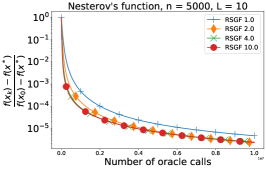
One can find our numerical results with tuning stepsizes for each method in Figures 3-5.

Refer to caption
Refer to caption
Refer to caption
Refer to caption
Refer to caption
Figure 3: Stepsize tuning for ARDD, RDD and RSGF applied to minimize Nesterov’s function (62). We use _E and _NE to define 2subscript2\ell_{2} and 1subscript1\ell_{1} proximal setups respectively (see (8) and (9) for the details). Numbers in labels in upper right corners denote different choices of γ𝛾\gamma that are used.
Refer to caption
Refer to caption
Refer to caption
Refer to caption
Refer to caption
Figure 4: Stepsize tuning for ARDD, RDD and RSGF applied to minimize Nesterov’s function (62). We use _E and _NE to define 2subscript2\ell_{2} and 1subscript1\ell_{1} proximal setups respectively (see (8) and (9) for the details). Numbers in labels in upper right corners denote different choices of γ𝛾\gamma that are used.
Refer to caption
Refer to caption
Refer to caption
Refer to caption
Refer to caption
Figure 5: Stepsize tuning for ARDD, RDD and RSGF applied to minimize Nesterov’s function (62). We use _E and _NE to define 2subscript2\ell_{2} and 1subscript1\ell_{1} proximal setups respectively (see (8) and (9) for the details). Number of oracle calls is divided by 107superscript10710^{7}. Numbers in labels in upper right corners denote different choices of γ𝛾\gamma that are used.

Our tests with Nesterov’s function show that for this problem ARDD_E and RDD_ work better with γ[32,64]𝛾3264\gamma\in[32,64] and RSGF shows the best performance with γ[4,10]𝛾410\gamma\in[4,10]. Interestingly, ARDD and RDD with p=1𝑝1p=1 require to choose γ𝛾\gamma significantly larger (of order 103104superscript103superscript10410^{3}-10^{4}) than for Euclidean methods in order to get competitive or even better convergence rate. Moreover, ARDD_E, RDD_E and RSGF disconverge for γ64,200,20𝛾6420020\gamma\geq 64,200,20 respectively. So, our empirical observation is as follows: ARDD and RDD with non-Euclidean proximal setup are able to converge with significantly larger stepsizes than its Euclidean counterpart.

We summarize best options for γ𝛾\gamma that we use in the experiments presented in Section 6 in Table 5.

ARDD_E ARDD_NE RDD_E RDD_NE RSGF
n=100𝑛100n=100 323232 200020002000 323232 120001200012000 101010
n=1000𝑛1000n=1000 323232 200020002000 646464 300030003000 444
n=5000𝑛5000n=5000 323232 100010001000 646464 300030003000 101010
Table 5: The optimal choices of γ𝛾\gamma for ARDD, RDD and RSGF applied to minimize Nesterov’s function (62) for different dimension n𝑛n.

C.2 Least squares problem

In addition to the tuning of γ𝛾\gamma in ARDD we also tried different options for L2subscript𝐿2L_{2}: instead of L2subscript𝐿2L_{2} from (64) we tried βAFr𝛽subscriptnorm𝐴𝐹𝑟\beta\cdot\frac{\|A\|_{F}}{\sqrt{r}} with different β𝛽\beta. We tried β=0.001,0.01,0.1,1,2,5𝛽0.0010.010.1125\beta=0.001,0.01,0.1,1,2,5 and 101010, but the best results were obtained for β=0.01𝛽0.01\beta=0.01. One can find our numerical results with tuning γ𝛾\gamma in Figure 6.

Refer to caption
Refer to caption
Refer to caption
Refer to caption
Refer to caption
Figure 6: Stepsize tuning for ARDD, RDD and RSGF applied to solve least squares problem (63). We use _E and _NE to define 2subscript2\ell_{2} and 1subscript1\ell_{1} proximal setups respectively (see (8) and (9) for the details). For all methods batch size m𝑚m equals 505050. By oracle call we mean one computation of functional value of a summand. Number of oracle calls is divided by 108superscript10810^{8}.

Besides m=50𝑚50m=50 we tried different batch sizes. In general, the behaviour of the considered methods was similar after proper parameters tuning.

References

  • [1] Alekh Agarwal, Ofer Dekel, and Lin Xiao. Optimal algorithms for online convex optimization with multi-point bandit feedback. In COLT 2010 - The 23rd Conference on Learning Theory, 2010.
  • [2] Zeyuan Allen-Zhu. Katyusha: The first direct acceleration of stochastic gradient methods. In Proceedings of the 49th Annual ACM SIGACT Symposium on Theory of Computing, STOC 2017, pages 1200–1205, New York, NY, USA, 2017. ACM. arXiv:1603.05953.
  • [3] Zeyuan Allen-Zhu, Zheng Qu, Peter Richtarik, and Yang Yuan. Even faster accelerated coordinate descent using non-uniform sampling. In Maria Florina Balcan and Kilian Q. Weinberger, editors, Proceedings of The 33rd International Conference on Machine Learning, volume 48 of Proceedings of Machine Learning Research, pages 1110–1119, New York, New York, USA, 20–22 Jun 2016. PMLR. First appeared in arXiv:1512.09103.
  • [4] A. S. Anikin, A. V. Gasnikov, P. E. Dvurechensky, A. I. Tyurin, and A. V. Chernov. Dual approaches to the minimization of strongly convex functionals with a simple structure under affine constraints. Computational Mathematics and Mathematical Physics, 57(8):1262–1276, 2017.
  • [5] John W. Barrett and Leonid Prigozhin. A quasi-variational inequality problem in superconductivity. Mathematical Models and Methods in Applied Sciences, 20(5):679–706, 2010.
  • [6] John W. Barrett and Leonid Prigozhin. Lakes and rivers in the landscape: A quasi-variational inequality approach. Interfaces and Free Boundaries, 16(2):269–296, 2014.
  • [7] Anastasia Bayandina, Pavel Dvurechensky, Alexander Gasnikov, Fedor Stonyakin, and Alexander Titov. Mirror descent and convex optimization problems with non-smooth inequality constraints. In Pontus Giselsson and Anders Rantzer, editors, Large-Scale and Distributed Optimization, chapter 8, pages 181–215. Springer International Publishing, 2018. arXiv:1710.06612.
  • [8] Anastasia Bayandina, Alexander Gasnikov, and Anastasia Lagunovskaya. Gradient-free two-points optimal method for non smooth stochastic convex optimization problem with additional small noise. Automation and remote control, 79(7), 2018. arXiv:1701.03821.
  • [9] Aaron Ben-Tal and Arkadi Nemirovski. Lectures on Modern Convex Optimization (Lecture Notes). Personal web-page of A. Nemirovski, 2015.
  • [10] Albert S. Berahas, Richard H. Byrd, and Jorge Nocedal. Derivative-free optimization of noisy functions via quasi-Newton methods. SIAM Journal on Optimization, 29(2):965–993, 2019.
  • [11] Albert S. Berahas, Liyuan Cao, Krzysztof Choromanski, and Katya Scheinberg. A theoretical and empirical comparison of gradient approximations in derivative-free optimization. arXiv:1905.01332, 2019.
  • [12] Albert S. Berahas, Liyuan Cao, and Katya Scheinberg. Global convergence rate analysis of a generic line search algorithm with noise. arXiv:1910.04055, 2019.
  • [13] Aleksandr Beznosikov, Eduard Gorbunov, and Alexander Gasnikov. Derivative-free method for composite optimization with applications to decentralized distributed optimization. IFAC-PapersOnLine, 2020. Accepted, arXiv:1911.10645.
  • [14] Aleksandr Beznosikov, Abdurakhmon Sadiev, and Alexander Gasnikov. Gradient-free methods for saddle-point problem. In A. Kononov and et al., editors, Mathematical Optimization Theory and Operations Research 2020, Cham, 2020. Springer International Publishing. accepted, arXiv:2005.05913.
  • [15] Lev Bogolubsky, Pavel Dvurechensky, Alexander Gasnikov, Gleb Gusev, Yurii Nesterov, Andrei M Raigorodskii, Aleksey Tikhonov, and Maksim Zhukovskii. Learning supervised pagerank with gradient-based and gradient-free optimization methods. In D. D. Lee, M. Sugiyama, U. V. Luxburg, I. Guyon, and R. Garnett, editors, Advances in Neural Information Processing Systems 29, pages 4914–4922. Curran Associates, Inc., 2016. arXiv:1603.00717.
  • [16] Raghu Bollapragada and Stefan M. Wild. Adaptive sampling quasi-Newton methods for derivative-free stochastic optimization. arXiv:1910.13516, 2019.
  • [17] R.P. Brent. Algorithms for Minimization Without Derivatives. Dover Books on Mathematics. Dover Publications, 1973.
  • [18] C. Cartis and K. Scheinberg. Global convergence rate analysis of unconstrained optimization methods based on probabilistic models. Mathematical Programming, 169(2):337–375, Jun 2018.
  • [19] Augustin Cauchy. Méthode générale pour la résolution des systémes d’équations simultanées. Comptes rendus hebdomadaires des séances de l’Académie des sciences, 55:536–538, 1847.
  • [20] Nicolò Cesa-bianchi, Alex Conconi, and Claudio Gentile. On the generalization ability of on-line learning algorithms. In T. G. Dietterich, S. Becker, and Z. Ghahramani, editors, Advances in Neural Information Processing Systems 14, pages 359–366. MIT Press, 2002.
  • [21] Yuwen Chen, Antonio Orvieto, and Aurelien Lucchi. An accelerated DFO algorithm for finite-sum convex functions. In Proceedings of the 37th International Conference on Machine Learning, Proceedings of Machine Learning Research. PMLR, 2020. (accepted), arXiv:2007.03311.
  • [22] Alexey Chernov, Pavel Dvurechensky, and Alexander Gasnikov. Fast Primal-Dual Gradient Method for Strongly Convex Minimization Problems with Linear Constraints, pages 391–403. Springer International Publishing, Cham, 2016.
  • [23] A. Conn, K. Scheinberg, and L. Vicente. Introduction to Derivative-Free Optimization. Society for Industrial and Applied Mathematics, 2009.
  • [24] Cong D. Dang and Guanghui Lan. Stochastic block mirror descent methods for nonsmooth and stochastic optimization. SIAM J. on Optimization, 25(2):856–881, April 2015.
  • [25] Olivier Devolder. Stochastic first order methods in smooth convex optimization. CORE Discussion Paper 2011/70, 2011.
  • [26] John C. Duchi, Michael I. Jordan, Martin J. Wainwright, and Andre Wibisono. Optimal rates for zero-order convex optimization: The power of two function evaluations. IEEE Trans. Information Theory, 61(5):2788–2806, 2015. arXiv:1312.2139.
  • [27] Darina Dvinskikh, Eduard Gorbunov, Alexander Gasnikov, Pavel Dvurechensky, and Cesar A. Uribe. On primal and dual approaches for distributed stochastic convex optimization over networks. In 2019 IEEE 58th Conference on Decision and Control (CDC), pages 7435–7440, 2019. arXiv:1903.09844.
  • [28] Darina Dvinskikh, Aleksandr Ogaltsov, Alexander Gasnikov, Pavel Dvurechensky, and Vladimir Spokoiny. On the line-search gradient methods for stochastic optimization. IFAC-PapersOnLine, 2020. Accepted, arXiv:1911.08380.
  • [29] P. E. Dvurechensky, A. V. Gasnikov, and A. A. Lagunovskaya. Parallel algorithms and probability of large deviation for stochastic convex optimization problems. Numerical Analysis and Applications, 11(1):33–37, Jan 2018. arXiv:1701.01830.
  • [30] Pavel Dvurechensky, Darina Dvinskikh, Alexander Gasnikov, César A. Uribe, and Angelia Nedić. Decentralize and randomize: Faster algorithm for Wasserstein barycenters. In S. Bengio, H. Wallach, H. Larochelle, K. Grauman, N. Cesa-Bianchi, and R. Garnett, editors, Advances in Neural Information Processing Systems 31, NeurIPS 2018, pages 10783–10793. Curran Associates, Inc., 2018. arXiv:1806.03915.
  • [31] Pavel Dvurechensky and Alexander Gasnikov. Stochastic intermediate gradient method for convex problems with stochastic inexact oracle. Journal of Optimization Theory and Applications, 171(1):121–145, 2016.
  • [32] Pavel Dvurechensky, Alexander Gasnikov, Evgenia Gasnikova, Sergey Matsievsky, Anton Rodomanov, and Inna Usik. Primal-dual method for searching equilibrium in hierarchical congestion population games. In Supplementary Proceedings of the 9th International Conference on Discrete Optimization and Operations Research and Scientific School (DOOR 2016) Vladivostok, Russia, September 19 - 23, 2016, pages 584–595, 2016. arXiv:1606.08988.
  • [33] Pavel Dvurechensky, Alexander Gasnikov, and Alexander Tiurin. Randomized similar triangles method: A unifying framework for accelerated randomized optimization methods (coordinate descent, directional search, derivative-free method). arXiv:1707.08486, 2017.
  • [34] Vaclav Fabian. Stochastic approximation of minima with improved asymptotic speed. Ann. Math. Statist., 38(1):191–200, 02 1967.
  • [35] Olivier Fercoq and Peter Richtárik. Accelerated, parallel, and proximal coordinate descent. SIAM Journal on Optimization, 25(4):1997–2023, 2015. First appeared in arXiv:1312.5799.
  • [36] A. V. Gasnikov and P. E. Dvurechensky. Stochastic intermediate gradient method for convex optimization problems. Doklady Mathematics, 93(2):148–151, Mar 2016.
  • [37] A. V. Gasnikov, P. E. Dvurechensky, M. E. Zhukovskii, S. V. Kim, S. S. Plaunov, D. A. Smirnov, and F. A. Noskov. About the power law of the pagerank vector component distribution. Part 2. The Buckley–Osthus model, verification of the power law for this model, and setup of real search engines. Numerical Analysis and Applications, 11(1):16–32, 2018.
  • [38] A. V. Gasnikov, E. V. Gasnikova, P. E. Dvurechensky, A. A. M. Mohammed, and E. O. Chernousova. About the power law of the pagerank vector component distribution. Part 1. Numerical methods for finding the pagerank vector. Numerical Analysis and Applications, 10(4):299–312, 2017.
  • [39] A. V. Gasnikov, E. A. Krymova, A. A. Lagunovskaya, I. N. Usmanova, and F. A. Fedorenko. Stochastic online optimization. single-point and multi-point non-linear multi-armed bandits. convex and strongly-convex case. Automation and Remote Control, 78(2):224–234, Feb 2017. arXiv:1509.01679.
  • [40] A. V. Gasnikov, A. A. Lagunovskaya, I. N. Usmanova, and F. A. Fedorenko. Gradient-free proximal methods with inexact oracle for convex stochastic nonsmooth optimization problems on the simplex. Automation and Remote Control, 77(11):2018–2034, Nov 2016. arXiv:1412.3890.
  • [41] Alexander Gasnikov, Pavel Dvurechensky, and Ilnura Usmanova. On accelerated randomized methods. Proceedings of Moscow Institute of Physics and Technology, 8(2):67–100, 2016. In Russian, first appeared in arXiv:1508.02182.
  • [42] Saeed Ghadimi and Guanghui Lan. Stochastic first- and zeroth-order methods for nonconvex stochastic programming. SIAM Journal on Optimization, 23(4):2341–2368, 2013. arXiv:1309.5549.
  • [43] Saeed Ghadimi, Guanghui Lan, and Hongchao Zhang. Mini-batch stochastic approximation methods for nonconvex stochastic composite optimization. Mathematical Programming, 155(1):267–305, 2016. arXiv:1308.6594.
  • [44] Eduard Gorbunov, Darina Dvinskikh, and Alexander Gasnikov. Optimal decentralized distributed algorithms for stochastic convex optimization. arXiv preprint arXiv:1911.07363, 2019.
  • [45] Eduard Gorbunov, Pavel Dvurechensky, and Alexander Gasnikov. An accelerated method for derivative-free smooth stochastic convex optimization. arXiv:1802.09022, 2018.
  • [46] Xiaowei Hu, Prashanth L.A., András György, and Csaba Szepesvari. (bandit) convex optimization with biased noisy gradient oracles. In Arthur Gretton and Christian C. Robert, editors, Proceedings of the 19th International Conference on Artificial Intelligence and Statistics, volume 51 of Proceedings of Machine Learning Research, pages 819–828, Cadiz, Spain, 09–11 May 2016. PMLR.
  • [47] Anatoli Juditsky and Yuri Nesterov. Deterministic and stochastic primal-dual subgradient algorithms for uniformly convex minimization. Stochastic Systems, 4(1):44–80, 2014.
  • [48] Dmitry Kamzolov, Pavel Dvurechensky, and Alexander V. Gasnikov. Universal intermediate gradient method for convex problems with inexact oracle. Optimization Methods and Software, 0(0):1–28, 2020. arXiv:1712.06036.
  • [49] K. Kim, Yu. Nesterov, V. Skokov, and B. Cherkasskii. Effektivnii algoritm vychisleniya proisvodnyh i ekstremalnye zadachi (efficient algorithm for calculation of derivatives and extreme problems). Ekonomika i matematicheskie metody, 20(2):309–318, 1984.
  • [50] Guanghui Lan. An optimal method for stochastic composite optimization. Mathematical Programming, 133(1):365–397, Jun 2012. Firs appeared in June 2008.
  • [51] Jeffrey Larson, Matt Menickelly, and Stefan M. Wild. Derivative-free optimization methods. Acta Numerica, 28:287–404, 2019.
  • [52] Yin Tat Lee and Aaron Sidford. Efficient accelerated coordinate descent methods and faster algorithms for solving linear systems. In Proceedings of the 2013 IEEE 54th Annual Symposium on Foundations of Computer Science, FOCS ’13, pages 147–156, Washington, DC, USA, 2013. IEEE Computer Society. First appeared in arXiv:1305.1922.
  • [53] Qihang Lin, Zhaosong Lu, and Lin Xiao. An accelerated proximal coordinate gradient method. In Z. Ghahramani, M. Welling, C. Cortes, N. D. Lawrence, and K. Q. Weinberger, editors, Advances in Neural Information Processing Systems 27, pages 3059–3067. Curran Associates, Inc., 2014. First appeared in arXiv:1407.1296.
  • [54] Boris S. Mordukhovich and Jiri V. Outrata. Coderivative analysis of quasi‐variational inequalities with applications to stability and optimization. SIAM Journal on Optimization, 18(2):389–412, 2007.
  • [55] A.S. Nemirovsky and D.B. Yudin. Problem Complexity and Method Efficiency in Optimization. J. Wiley & Sons, New York, 1983.
  • [56] Yurii Nesterov. Introductory Lectures on Convex Optimization: a basic course. Kluwer Academic Publishers, Massachusetts, 2004.
  • [57] Yurii Nesterov. Efficiency of coordinate descent methods on huge-scale optimization problems. SIAM Journal on Optimization, 22(2):341–362, 2012. First appeared in 2010 as CORE discussion paper 2010/2.
  • [58] Yurii Nesterov. Universal gradient methods for convex optimization problems. Mathematical Programming, 152(1):381–404, 2015.
  • [59] Yurii Nesterov, Alexander Gasnikov, Sergey Guminov, and Pavel Dvurechensky. Primal-dual accelerated gradient methods with small-dimensional relaxation oracle. Optimization Methods and Software, pages 1–28, 2020. arXiv:1809.05895.
  • [60] Yurii Nesterov and Vladimir Spokoiny. Random gradient-free minimization of convex functions. Found. Comput. Math., 17(2):527–566, April 2017. First appeared in 2011 as CORE discussion paper 2011/16.
  • [61] Yurii Nesterov and Sebastian U. Stich. Efficiency of the accelerated coordinate descent method on structured optimization problems. SIAM Journal on Optimization, 27(1):110–123, 2017. First presented in May 2015 http://www.mathnet.ru:8080/PresentFiles/11909/7_nesterov.pdf.
  • [62] Warren B. Powell. A unified framework for stochastic optimization. European Journal of Operational Research, 275(3):795 – 821, 2019.
  • [63] Leonid Prigozhin. Variational model of sandpile growth. European Journal of Applied Mathematics, 7(3):225–235, 1996.
  • [64] H. H. Rosenbrock. An automatic method for finding the greatest or least value of a function. The Computer Journal, 3(3):175–184, 1960.
  • [65] Shai Shalev-Shwartz and Tong Zhang. Accelerated proximal stochastic dual coordinate ascent for regularized loss minimization. In Eric P. Xing and Tony Jebara, editors, Proceedings of the 31st International Conference on Machine Learning, volume 32 of Proceedings of Machine Learning Research, pages 64–72, Bejing, China, 22–24 Jun 2014. PMLR. First appeared in arXiv:1309.2375.
  • [66] Ohad Shamir. An optimal algorithm for bandit and zero-order convex optimization with two-point feedback. Journal of Machine Learning Research, 18:52:1–52:11, 2017. First appeared in arXiv:1507.08752.
  • [67] James C. Spall. Introduction to Stochastic Search and Optimization. John Wiley & Sons, Inc., New York, NY, USA, 1 edition, 2003.
  • [68] Fedor Stonyakin, Alexander Tyurin, Alexander Gasnikov, Pavel Dvurechensky, Artem Agafonov, Darina Dvinskikh, Dmitry Pasechnyuk, Sergei Artamonov, and Victorya Piskunova. Inexact relative smoothness and strong convexity for optimization and variational inequalities by inexact model. arXiv:2001.09013, 2020.
  • [69] Fedor S. Stonyakin, Darina Dvinskikh, Pavel Dvurechensky, Alexey Kroshnin, Olesya Kuznetsova, Artem Agafonov, Alexander Gasnikov, Alexander Tyurin, César A. Uribe, Dmitry Pasechnyuk, and Sergei Artamonov. Gradient methods for problems with inexact model of the objective. In Michael Khachay, Yury Kochetov, and Panos Pardalos, editors, Mathematical Optimization Theory and Operations Research, pages 97–114, Cham, 2019. Springer International Publishing. arXiv:1902.09001.
  • [70] E. A. Vorontsova, A. V. Gasnikov, E. A. Gorbunov, and P. E. Dvurechenskii. Accelerated gradient-free optimization methods with a non-euclidean proximal operator. Automation and Remote Control, 80(8):1487–1501, 2019.
  • [71] R. E. Wengert. A simple automatic derivative evaluation program. Commun. ACM, 7(8):463–464, August 1964.