Comparison of Travel-Time and Amplitude Measurements for Deep-Focusing Time–Distance Helioseismology

iint iiint

1 Introduction

Time–distance helioseismology (Duvall et al., 1993) is a branch of local helioseismology (e.g. Gizon and Birch, 2005) that aims at probing the complex subsurface structures of the solar interior. The time–distance method measures the travel times of acoustic waves between any pair of points on the solar surface from the cross-covariance function of the observed oscillation signals. Seismic travel times contain information about the local physical properties of the medium and have thus been broadly used in helioseismology (e.g. Gizon and Birch, 2002; Birch, Kosovichev, and Duvall, 2004; Gizon, Birch, and Spruit, 2010).

A consistent issue with local helioseismology is the signal-to-noise ratio. When examining near-surface structures such as supergranular flows (Duvall et al., 1996; Langfellner, Gizon, and Birch, 2015), averaging is typically performed around an annulus, where the cross-covariance is calculated between the center point and the average signal in the annulus. This technique is highly sensitive to near-surface perturbations. To probe greater depths, one would seek a different averaging technique that has peak sensitivity at any chosen target depth. Such a technique is known as deep-focusing and was first described by Duvall (1995), who outlined a procedure in which points on the surface are chosen such that a large number of connecting ray paths intersect at the target (focus) point, with the expectation that sensitivity is large near the target depth. The deep-focusing time–distance technique has been employed to study the meridional flow in the solar interior (e.g. Hartlep et al., 2013; Zhao et al., 2013) and sunspot structure (e.g. Moradi and Hanasoge, 2010). Jensen (2001) investigated the application of the deep-focusing method to improve inversions for large sunspots. Using the Rytov approximation, he found sensitivity in a shell around the target point but zero sensitivity at the target point, consistent with wavefront healing seen in the Born approximation in geophysics and helioseismology. To resolve this drawback, Hughes, Pijpers, and Thompson (2007) suggested an optimized technique for deep focusing that allocates weightings for each measurement. They obtained improvements in the results by considering travel-time measurements of synthetic experiments.

In addition to the travel times, the cross-covariance function contains additional information that may be of use to helioseismology. For instance, in terrestrial seismology cross-covariance amplitudes have been used to characterize seismic waves (e.g. Nolet, Dahlen, and Montelli, 2005). The importance of the amplitudes was examined by Dalton, Hjörleifsdóttir, and Ekström (2014), who concluded that assumptions and simplifications in the measurement of surface-wave amplitudes affect the attenuation structure found through inversions. Moreover, Dahlen and Baig (2002) investigated the Fréchet sensitivity kernels using the geometrical ray approximation for travel-time and amplitude measurements. They found a maximum sensitivity along the point-to-point ray path when examining the amplitude of seismic-wave cross-correlation. In contrast to travel times, few studies have considered the amplitude measurements of the cross-covariance function in helioseismology. Liang et al. (2013) measured the spatial maps of wave travel times and amplitudes from the cross-covariance function of the wave field around a sunspot in the NOAO Active Region 9787. Using 2D ray theory, they observed an amplitude reduction that was attributed to the defocusing of wave energy by the fast-wave-speed perturbation in the sunspot. Recent work by Nagashima et al. (2017) described a linear procedure to measure the amplitude of the cross-covariance function of solar oscillations. This linear relation between the cross-covariance function and the amplitude allows the derivation of Born sensitivity kernels using the procedure of Gizon and Birch (2002), which provides a straightforward interpretation for the amplitude measurements.

The deep-focusing time–distance technique using amplitude measurements is lacking in time–distance helioseismology. Furthermore, the deep-focusing analysis has been considered only using the ray theory, which is a high-frequency approximation and does not take into account finite-wavelength effects. As a result, the ray approximation may be inaccurate for amplitude calculations (e.g. Tong et al., 1998). In this study, we use the deep-focusing time–distance technique to compare signal and noise for travel-time and amplitude measurements under the Born approximation. Section sec:cross-covariance describes the definition of travel-time and amplitude measurements and explains the deep-focusing technique and the noise model. The setup and derivation of sensitivity kernels are explained in Section sec:toy_problem and the results are presented in Section sec:results. Conclusions are given in Section sec:summary.

2 Travel-Time and Amplitude Measurements

sec:cross-covariance

2.1 Definitions

In time–distance helioseismology, one uses the cross-covariance function between the oscillation signals observed at any two points [$\bm{r}_{1}$ and $\bm{r}_{2}$] on the solar surface to recover the desired information within the relevant wave-field observable. In general, we observe the line-of-sight velocity $[\phi]$ and define the temporal cross-covariance function for surface locations $\bm{r}_{1}$ and $\bm{r}_{2}$ as

$$C(\bm{r}_{1},\bm{r}_{2},t)=\frac{1}{T}\int_{-T/2}^{T/2}\phi(\bm{r}_{1},t^{\prime})\phi(\bm{r}_{2},t^{\prime}+t)\,\mathrm{d}t^{\prime},\ilabel{eq:cross-cov_{g}eneral}$$ (1)

where $t$ is the time lag and $T$ is the duration of observation. Considering small changes to a reference solar model, one can define the incremental travel time $[\delta\tau]$ and relative amplitude $[\delta a]$ between the observed $[C(\bm{r}_{1},\bm{r}_{2};t)]$ and reference $[C_{0}(\bm{r}_{1},\bm{r}_{2};t)]$ cross-covariances as

$$\delta\tau(\bm{r}_{1},\bm{r}_{2}) = \int_{-T/2}^{T/2}W_{\tau}(\bm{r}_{1},\bm{r}_{2},t)\,\delta C(\bm{r}_{1},\bm{r}_{2},t)\,\mathrm{d}t,$$ (2)

$$\delta a(\bm{r}_{1},\bm{r}_{2}) = \int_{-T/2}^{T/2}W_{a}(\bm{r}_{1},\bm{r}_{2},t)\,\delta C(\bm{r}_{1},\bm{r}_{2},t)\,\mathrm{d}t,$$ (3)

where

$$\delta C(\bm{r}_{1},\bm{r}_{2},t)=C(\bm{r}_{1},\bm{r}_{2},t)-C_{0}(\bm{r}_{1},\bm{r}_{2},t).$$ (4)

The above linear relations between the measurements and the cross-covariance function are specified via the weighting functions $[W]$ given by Nagashima et al. (2017):

$$W_{\tau}(t) = -\frac{w(t)\partial_{t}C_{0}(t)}{\int_{-T/2}^{T/2}w(t^{\prime})[\partial_{t^{\prime}}C_{0}(t^{\prime})]^{2}\mathrm{d}t^{\prime}},$$ (5)

$$W_{a}(t) = \frac{w(t)C_{0}(t)}{\int_{-T/2}^{T/2}w(t^{\prime})[C_{0}(t^{\prime})]^{2}\mathrm{d}t^{\prime}},$$ (6)

where $w(t)$ is a window function that may select the first-arrival wave packet. With this definition of the weighting function $[W_{a}]$ the relative amplitude $[\delta a]$ is dimensionless.

Throughout this article, we use $q$ to denote either the travel-time $[\tau]$ or the amplitude measurement $[a]$. Using this compact notation, we write

$$\delta q(\bm{r}_{1},\bm{r}_{2})=\int_{-T/2}^{T/2}W_{q}(\bm{r}_{1},\bm{r}_{2},t)\delta C(\bm{r}_{1},\bm{r}_{2},t)\,\mathrm{d}t,\quad\text{ for }q\in\{\tau,a\}.\ilabel{eq:travel_{t}ime_{g}eneral}$$ (7)

2.2 Deep-Focusing Averages

sec:Deep_Foc The basic idea of the deep-focusing technique is to obtain high sensitivity to a physical quantity by focusing at a given target point. To do so, we consider a set of pairs of points on the solar surface such that the ray paths (straight lines for a homogeneous medium) intersect at a chosen target point. As an example, Figure fig:points illustrates how these pairs of points could be distributed on the surface of the near-side of the Sun. In a solar case, the ray paths would be curved due to the sound-speed stratification.

For any desired target point $[\bm{r}_{t}]$ in the solar interior, we define the averaged travel-time and amplitude perturbations as

$$\overline{\delta q}(\bm{r}_{t})=\frac{1}{N}\sum_{i=1}^{N}\delta q_{i}(\bm{r}_{t}),\quad q\in\{\tau,a\},\ilabel{eq:ave_{t}ravel_{t}ime}$$ (8)

where $\delta q_{i}(\bm{r}_{t})$ represents the point-to-point measurement between the points $\bm{r}_{i}$ and $\bm{r}^{\prime}_{i}$ chosen such that the ray path intersects at the focus point $\bm{r}_{t}$,

$$\delta q_{i}(\bm{r}_{t})=\delta q(\bm{r}_{i},\bm{r}^{\prime}_{i}).\ilabel{eq:travel_{t}ime_{i}j}$$ (9)

The observations points $\bm{r}_{i}$ and $\bm{r}_{i}^{\prime}$ are on a sphere of radius $\mathrm{R_{\odot}}$ and have coordinates $\bm{r}_{i}=(\mathrm{R_{\odot}},\theta_{i},\phi_{i})$ and $\bm{r}^{\prime}_{i}=(\mathrm{R_{\odot}},{\theta}^{\prime}_{i},\phi^{\prime}_{i})$ in the spherical-polar coordinate system whose polar axis contains the target point (depicted in Figure fig:points). The index $i$ spans $[1,N]$, where $N=N_{\theta}N_{\phi}$ is the total number of pairs of points, with $N_{\theta}$ the number of colatitudes and $N_{\phi}$ the number of longitudes. Each index $i$ is associated with a pair of indices $(i_{\theta},i_{\phi})\in[1,N_{\theta}]\times[1,N_{\phi}]$, where the first index refers to the colatitudes $\theta_{i_{\theta}}$ and $\theta^{\prime}_{i_{\theta}}=\Delta-\theta_{i_{\theta}}$ (where $\Delta$ is the colatitude difference between the two observation points in a pair) and the second index refers to the uniformly-spaced azimuths $\phi_{i_{\phi}}={2\pi}(i_{\phi}-1)/N_{\phi}$ and $\phi_{i_{\phi}}^{\prime}=\phi_{i_{\phi}}+\pi$. The range of colatitudes $\theta_{1}\leq\theta\leq\theta_{N_{\theta}}$ defines the extent of the pupil. Choosing a maximum value $\theta_{N_{\theta}}=65^{\circ}$, the value of $\theta_{1}$ then depends on the target depth. At a fixed longitude, the colatitudes of the points within the pupil are chosen such that the angle between neighboring ray paths is uniform.

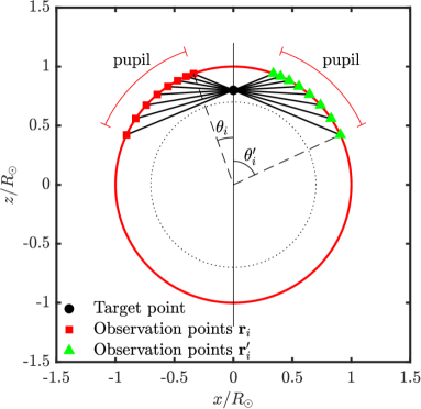
Figure 1.: Sketch depicting the location of the observation points $\bm{r}_{i}$ (red squares) and $\bm{r}^{\prime}_{i}$ (green triangles) inside the pupil. The points are chosen such that the ray paths (black lines) intersect at a focus point at $z_{t}=0.8\,\mathrm{R_{\odot}}$ (black dot). The dotted circle has a radius of $0.7\,\mathrm{R_{\odot}}$.fig:points

2.3 Noise Model

sec:noise_model Here we describe the noise in the averaged measurements for travel time and amplitude. Random noise in helioseismology is due to the stochastic excitation of acoustic waves by turbulent convection. The noise model developed by Gizon and Birch (2004) is based on the reasonable assumption that the reference wave field $[\phi_{0}]$ is described by a stationary Gaussian random process.

The variance of the averaged travel-time or amplitude measurement is given by

$$\sigma^{2}_{q}=\textrm{Var}\left[\,\overline{\delta q}\,\right]=\frac{1}{N^{2}}\sum_{i=1}^{N}\sum_{j=1}^{N}\textrm{Cov}[\delta q_{i},\delta q_{j}].\ilabel{eq:std_{t}au}$$ (10)

The covariance between any two measurements [$\textrm{Cov}[\delta q_{i},\delta q_{j}]$] depends on the reference cross-covariance function in the frequency domain,

$$C_{0}(\omega)=\frac{1}{2\pi}\int_{-{T}/{2}}^{{T}/{2}}C_{0}(t)e^{\textrm{i}\omega t}\,\mathrm{d}t,\ilabel{C_{0}{}_{f}req}$$ (11)

and on the weighting functions $[W_{q}]$. Fournier et al. (2014) showed that the covariance is explicitly given by

$$\textrm{Cov}[\delta q_{i},\delta q_{j}]=\frac{(2\pi)^{3}}{T}\int_{-\omega_{\rm max}}^{\omega_{\rm max}}\mathrm{d}\omega W_{q}^{*}(\bm{r}_{i},\bm{r}^{\prime}_{i},\omega)\left[W_{q}(\bm{r}_{j},\bm{r}^{\prime}_{j},\omega)C_{0}(\bm{r}^{\prime}_{i},\bm{r}^{\prime}_{j},\omega)\right.\\ \left.\times C_{0}(\bm{r}_{i},\bm{r}_{j},\omega)+W_{q}^{*}(\bm{r}_{j},\bm{r}^{\prime}_{j},\omega)C_{0}(\bm{r}_{j},\bm{r}^{\prime}_{i};\omega)C_{0}(\bm{r}_{i},\bm{r}^{\prime}_{j},\omega)\right],\ilabel{eq:noise_{c}ov_{t}au}$$ (12)

where $\omega_{\rm max}=\pi/h_{t}$ is the Nyquist frequency and $h_{t}$ is the temporal cadence. The star denotes complex conjugation. Note that the noise covariance was originally derived for travel-time measurements, but it is easily extended to the amplitude measurements due to the linearity between $\delta a$ and $\delta C$.

3 Travel-Time and Amplitude Sensitivity Kernels for Sound-Speed Perturbations to a Uniform Background Medium

sec:toy_problem

3.1 Wave Equation and Reference Green’s Function

We consider the wave equation at angular frequency $\omega$,

$$\mathcal{L}\phi(\bm{r},\omega)=s(\bm{r},\omega),$$ (13)

where the wave operator is

$$\mathcal{L}=\nabla^{2}+k^{2}(\bm{r},\omega)\ilabel{eq:wave_{o}perator}$$ (14)

and the wave number is given by

$$k(\bm{r},\omega)=\frac{\omega}{c(\bm{r})}\left(1+\textrm{i}\gamma\right),$$ (15)

where $c(\bm{r})$ is the sound speed and $\gamma$ is a constant number that accounts for attenuation. The random source of excitation $s(\bm{r},\omega)$ is assumed to be stationary, uniformly distributed and spatially uncorrelated throughout the medium. Under these conditions, the expectation value of the cross-covariance function can be related directly to the imaginary part of the Green’s function in the frequency domain (e.g. Gizon et al., 2017)

$$\langle C(\omega)\rangle=\frac{\Pi(\omega)}{\omega}\mbox{Im}\,G(\bm{r},\bm{r}^{\prime},\omega),\ilabel{eq:cross_{c}ov}$$ (16)

where the function $\Pi(\omega)$ is related to the frequency dependence of the source covariance. The angle brackets $\langle\ \rangle$ represent the expectation value of a stochastic quantity.

We consider a background medium with the reference wave number

$$k_{0}(\omega)=\frac{\omega}{c_{0}}\left(1+\textrm{i}\gamma\right),\ilabel{eq:ref_{k}}$$ (17)

where the reference sound speed is constant $c_{0}$. The reference Green’s function is solution of $\mathcal{L}_{0}G_{0}(\bm{r},\bm{r}^{\prime})=\delta(\bm{r}-\bm{r}^{\prime})$ where $\mathcal{L}_{0}=\nabla^{2}+k_{0}^{2}$ is the reference wave operator. Using a Sommerfeld radiation condition to avoid incoming waves at infinity, the expression for $G_{0}$ is

$$G_{0}(\bm{r},\bm{r}^{\prime})=-\frac{e^{\textrm{i}k_{0}\|\bm{r}-\bm{r}^{\prime}\|}}{4\pi\|\bm{r}-\bm{r}^{\prime}\|}.\ilabel{eq:analytic_{G}reen}$$ (18)

This simple analytic expression motivates the choice that we have made of a uniform medium.

3.2 Perturbation to the Cross-Covariance Function

sec:Born approximation In this section we compute the perturbation to the cross-covariance $[\delta C=C-C_{0}]$ due to a small perturbation in sound speed $[\delta c(\bm{r})=c(\bm{r})-c_{0}]$. Using Equation eq:cross_cov, the expectation value of $\delta C$ is related to the perturbation to the Green’s function,

$$\langle\delta C(\omega)\rangle=\langle C(\omega)\rangle-C_{0}(\omega)=\frac{\Pi(\omega)}{\omega}\mbox{Im}\,(\delta G).\ilabel{eq:smartgreen}$$ (19)

Under the first-order Born approximation we have

$$\mathcal{L}_{0}\delta G(\bm{r},\bm{r}^{\prime},\omega)=-\delta\mathcal{L}G_{0}(\bm{r},\bm{r}^{\prime},\omega),\ilabel{eq:Born}$$ (20)

where $\delta\mathcal{L}=-2k_{0}^{2}\delta c(\bm{r})/c_{0}$ is the perturbation to the wave operator caused by the perturbations in the sound speed $\delta c$. According to Equation eq:Born, the Born approximation is an equivalent-source description of wave interaction. Using $G_{0}$ to solve for $\delta G$, we find

$$\delta G(\bm{r}_{i},\bm{r}^{\prime}_{i},\omega)=\int_{V}G_{0}(\bm{r}_{i},\bm{r},\omega)\,2k_{0}^{2}\frac{\delta c(\bm{r})}{c_{0}}\,G_{0}(\bm{r},\bm{r}^{\prime}_{i},\omega)\,\mathrm{d}^{3}\bm{r},\ilabel{eq:deltaG}$$ (21)

where $V$ is the computational domain, including the full sphere. It follows that the perturbation to the cross-covariance between the points $\bm{r}_{i}$ and $\bm{r}^{\prime}_{i}$ is

$$\langle\delta C_{i}(\omega)\rangle=\int_{V}\mathscr{C}_{i}(\bm{r},\omega)\frac{\delta c(\bm{r})}{c_{0}}\,\mathrm{d}^{3}\bm{r},\ilabel{eq:deltaC}$$ (22)

where $\mathscr{C}_{i}(\bm{r},\omega)$ is defined as

$$\mathscr{C}_{i}(\bm{r},\omega)=\frac{2\Pi(\omega)}{\omega}\mbox{ Im}\left[k_{0}^{2}G_{0}(\bm{r},\bm{r}_{i},\omega)G_{0}(\bm{r},\bm{r}^{\prime}_{i},\omega)\right],\ilabel{eq:kernel_{C}}$$ (23)

where we used seismic reciprocity (the Green’s function is unchanged upon exchanging source and receiver). Equation eq:kernel_C shows that to compute the perturbation to the cross-covariance we need to compute a product of two Green’s functions, one with a source at $\bm{r}_{i}$ and the other one with a source at $\bm{r}^{\prime}_{i}$.

3.3 Travel-Time and Amplitude Sensitivity Kernels

With the expression in hand for the perturbation to the cross-covariance, we now extract the travel-time and amplitude perturbations from the cross-covariance function. Using Equation eq:travel_time_general and Equation eq:deltaC, the expectation value of the perturbation to the travel time $[\langle\delta\tau_{i}\rangle]$ and to the amplitude $[\langle\delta a_{i}\rangle]$ is given by

$$\langle\delta q_{i}\rangle=2\pi\int_{-\omega_{\rm max}}^{\omega_{\rm max}}W_{q}^{*}(\omega)\langle\delta C_{i}(\omega)\rangle\mathrm{d}\omega=\int_{V}K_{i}^{q}(\bm{r})\frac{\delta c(\bm{r})}{c_{0}}\mathrm{d}^{3}\bm{r},\quad q\in\{\tau,a\},\ilabel{eq:travel_{t}ime_{i}}$$ (24)

where $K^{q}$ are the point-to-point sensitivity kernels

$$K_{i}^{q}(\bm{r})=2\pi\int_{-\omega_{\rm max}}^{\omega_{\rm max}}W_{q}^{*}(\omega)\mathscr{C}_{i}(\bm{r},\omega)\mathrm{d}\omega.\ilabel{eq:kernel_{w}}$$ (25)

Next we need to average the measurements for the deep-focusing technique as explained in Section sec:Deep_Foc. Using Equation eq:ave_travel_time, the expectation values of the averaged travel-time $\langle\overline{\delta\tau}\rangle$ and amplitude $\langle\overline{\delta a}\rangle$ perturbations can be written as

$$\langle\overline{\delta q}(\bm{r}_{t})\rangle=\frac{1}{N}\sum_{i=1}^{N}\langle\delta q_{i}(\bm{r}_{t})\rangle=\int_{V}\overline{K^{q}}(\bm{r};\bm{r}_{t})\frac{\delta c(\bm{r})}{c_{0}}\mathrm{d}^{3}\bm{r},\quad q\in\{\tau,a\},\ilabel{eq:ave_{t}ravel_{t}ime_{k}ernel}$$ (26)

where $\overline{K^{q}}(\bm{r};\bm{r}_{t})$ are the deep-focusing sensitivity kernels targeting a point at $\bm{r}_{t}$ defined by

$$\overline{K^{q}}(\bm{r};\bm{r}_{t})=\frac{1}{N}\sum_{i=1}^{N}K_{i}^{q}(\bm{r}),\quad q\in\{\tau,a\}.\ilabel{eq:Ave_{k}{}_{t}au}$$ (27)

4 Example Calculations

sec:results

4.1 Choice of Numerical Values and Parameters

In the following, the value of the reference sound speed is $c_{0}=10^{5}$ $\rm{m\,s}^{-1}$, the wave attenuation parameter is $\gamma=10^{-3}$, and $\mathrm{R_{\odot}=696}$ Mm. The frequency dependence of the source covariance is chosen to be a Gaussian profile,

$$\Pi(\omega)=\exp\left(-\frac{(\left|\omega\right|-\omega_{0})^{2}}{2\sigma^{2}}\right),\ilabel{eq:Pi_{f}unc_{G}auss}$$ (28)

where $\omega_{0}/2\pi=3$ mHz and $\sigma/2\pi=1$ mHz. In our computations, we chose a temporal cadence $h_{t}=45$ s, i.e. the Solar Dynamics Observatory (SDO)/ Helioseismic and Magnetic Imager (HMI) cadence.

To compute the travel time and the amplitude, we have to define the window function $w$ in Equations eq:weighting_func – eq:weighting_func_amp. Since in this setup the cross-covariance function has a single branch, we chose a Heaviside step function:

$$w(t)=\begin{cases}1&\textrm{if}\quad t>0,\\ 0&\textrm{otherwise}.\end{cases}\ilabel{eq:window_{f}unc}$$ (29)

Using the analytic expression for the Green’s function (Equation eq:analytic_Green) we obtain the reference cross-covariance $[C_{0}]$ (Equation eq:cross_cov). Figure fig:C_Wtau_Wamp shows the travel-time and amplitude weighting functions [$W_{\tau}$ and $W_{a}$] as a function of time for a pair of points separated by a distance of $D=1.2\,\mathrm{R_{\odot}}$. The function $W_{a}$ is proportional to $C_{0}$ as stated by Equation eq:weighting_func_amp, while $W_{\tau}$ is proportional to the temporal derivative of $C_{0}$ (Equation eq:weighting_func) and is thus shifted by one-fourth of a period.

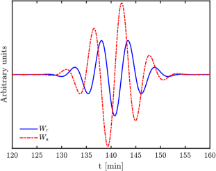
Figure 2.: Sketch of the weighting functions for measuring travel times $[W_{\tau}]$ and cross-covariance amplitudes $[W_{a}]$. The function $W_{a}$ is proportional to the unperturbed cross-covariance function $[C_{0}]$. In this example, the two observation points are separated by a distance $D=1.2\,\mathrm{R_{\odot}}$. The scalings for the functions $W_{\tau}$ and $W_{a}$ that are shown here are arbitrary as the two functions have different units.fig:C˙Wtau˙Wamp

4.2 Point-to-point Sensitivity Kernels

Using Equation eq:kernel_w, we compute the point-to-point travel-time and amplitude sensitivity kernels for sound-speed perturbations with a pair of points separated by $1.2\,\mathrm{R_{\odot}}$. Cross-sections through the point-to-point sensitivity kernels for the sound speed are shown in Figure fig:single_kernels. As already discussed in geophysics (Dahlen and Baig, 2002) and in helioseismology (Gizon and Birch, 2002), the travel-time kernel $[K^{\tau}]$ has small values along the geometrical ray path and the largest absolute values in the surrounding first Fresnel zone; see Figure fig:single_kernels(a). The kernel changes sign multiple times away from the ray path when crossing higher-order Fresnel zones. One the other hand, the amplitude sensitivity kernel for sound-speed takes maximum absolute values along the ray path (Nolet, Dahlen, and Montelli, 2005), see Figure fig:single_kernels(b). For a uniform background model, both point-to-point kernels are axially symmetric about the ray path. The total volume integrals of the two-point kernels are negative, $\int K^{\tau}(\bm{r})\mathrm{d}^{3}\bm{r}\approx-8500$ s and $\int K^{a}(\bm{r})\mathrm{d}^{3}\bm{r}\approx-1.2$, which means that a uniform reduction in sound speed leads to a longer travel time and a larger cross-covariance amplitude.

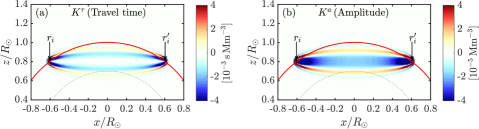
Figure 3.: 2D cross-sections ($y=0$) through the point-to-point kernels for sound-speed perturbations: (a) travel-time kernel $K^{\tau}(\bm{r})$ and (b) amplitude kernel $K^{a}(\bm{r})$. The pair of points ($\bm{r}_{i},\bm{r}^{\prime}_{i}$) on the surface are separated by $D=1.2\,\mathrm{R_{\odot}}$. The dotted circle highlights radius $r=0.7\,\mathrm{R_{\odot}}$.fig:single˙kernels

4.3 Deep-Focusing Sensitivity Kernels

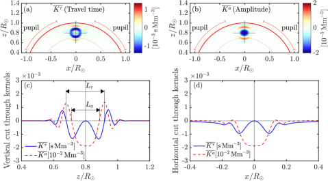
Figure 4.: 2D cross-sections ($y=0$) through the 3D deep-focusing (a) sensitivity kernel for $\overline{\delta\tau}$ and (b) sensitivity kernel for $\overline{\delta a}$ averaged over the $N=N_{\theta}N_{\phi}$ observation points, where $N_{\theta}=158$ and $N_{\phi}=793$. The cross shows the target location, $x_{t}=y_{t}=0$, $z_{t}=0.8\,\mathrm{R_{\odot}}$ which corresponds to the separation distance, $D=1.2\,\mathrm{R_{\odot}}$ and the dots are situated at the surface at $z=0.7\,\mathrm{R_{\odot}}$. (c) Vertical ($x=0$, $y=0$) and (d) horizontal ($y=0$, $z=0.8\,\mathrm{R_{\odot}}$) cuts of the sensitivity kernels. $L_{\tau}$ and $L_{a}$ are the vertical widths of the deep-focusing kernels for travel time and amplitude, respectively.fig:aveKernels

With the point-to-point kernels for sound-speed perturbations in hand, we compute the deep-focusing sensitivity kernels for averaged travel time and amplitude using Equation eq:Ave_k_tau. We consider all pairs of points in a pupil such that their ray paths intersect at a given target point along the $z$-axis. Neighboring observation points are separated in colatitude by a distance of approximately $\lambda_{\rm min}/4\approx 5$ Mm ($0.41^{\circ}$), where $\lambda_{\rm min}$ is the minimum wavelength used in this calculation. For a target point at radius $z_{t}=0.8\,\mathrm{R_{\odot}}$, Figures fig:aveKernels(a) and fig:aveKernels(b) show 2D cross-sections ($y=0$) through the deep-focusing sound-speed sensitivity kernels for $\overline{\delta\tau}$ and $\overline{\delta a}$. For travel-time measurements, the sensitivity is restricted to a shell surrounding the target location. In the case of amplitude measurements, the sensitivity is highly localized at the target point. This is a direct consequence of the structure of the point-to-point kernels depicted in Figure fig:single_kernels. Figure fig:aveKernels_nearSurface shows the same bottom panels as in Figure fig:aveKernels, but for a target point near the surface, $z_{t}=0.95\,\mathrm{R_{\odot}}$. This target point leads to a shorter separation distance: $D=0.63\,\mathrm{R_{\odot}}$.

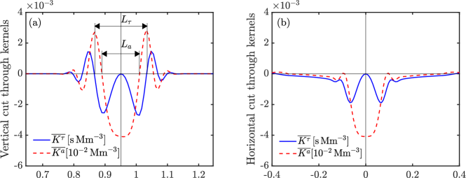
Figure 5.: (a) Vertical ($x=0$, $y=0$) and (b) horizontal ($y=0$, $z=0.95\,\mathrm{R_{\odot}}$) cuts of the sensitivity kernels for $\overline{\delta\tau}$ and $\overline{\delta a}$ for the target location, $x_{t}=y_{t}=0$, $z_{t}=0.95\,\mathrm{R_{\odot}}$ which corresponds to the shorter separation distance, $D=0.63\,\mathrm{R_{\odot}}$.fig:aveKernels˙nearSurface

4.4 Kernel Widths as Functions of Target Depth

sec.fresnel

The vertical widths of the deep-focusing sensitivity kernels for travel time [$L_{\tau}$] and amplitude [$L_{a}$] are defined in Figure fig:aveKernels(c). This width indicates the extent of the central regions of a kernel, within which it keeps the same (negative) sign. The smaller $L_{\tau}$ (or $L_{a}$), the higher the spatial resolution of the travel-time (or amplitude) deep-focusing technique.

In Figure fig:L_width the widths $L_{\tau}$ and $L_{a}$ are plotted as functions of the target radius $z_{t}$. The sensitivity kernels for amplitude measurements are better localized than those for travel-time measurements, at all depths, with $L_{a}\approx 0.7L_{\tau}$. Furthermore $L_{\tau}$ and $L_{a}$ increase with target depth.

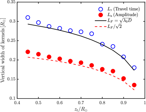
Figure 6.: Vertical width of the deep-focusing sensitivity kernels for travel time ($L_{\tau}$, open circles) and amplitude ($L_{a}$, full circles) as a function of target position. The solid and dashed curves show the simple models described in Section sec.fresnel. The width of the first Fresnel zone is approximately $L_{F}=\sqrt{\lambda_{0}D}$, where $D$ is the distance between the two points and $\lambda_{0}=33.3$ Mm is the wavelength at frequency $3$ mHz. fig:L˙width

In order to better understand the data points, we consider a simplified version of the model presented in Section sec:Born approximation. For a single sound-speed scatterer (volume $\mathrm{d}V$) at position $\bm{r}$ in the mid-plane, the cross-covariance between observation points $\bm{r}_{i}$ and $\bm{r}_{i}^{\prime}$ can be written

eq.phitot$$C(\bm{r}_{i},\bm{r}_{i}^{\prime}) \propto {\rm Im}\left[G_{0}(\bm{r}_{i}^{\prime},\bm{r}_{i})+\tilde{\epsilon}G_{0}(\bm{r}_{i}^{\prime},\bm{r})G_{0}(\bm{r},\bm{r}_{i})\right],\quad\tilde{\epsilon}=2k_{0}^{2}\frac{\delta c}{c_{0}}\mathrm{d}V,$$ (30)

$$\propto {\rm Im}\left[G_{0}(\bm{r}_{i}^{\prime},\bm{r}_{i})\left(1-\epsilon\,\rm e^{\textrm{i}\Delta\phi}\right)\right],\qquad\qquad\;\epsilon\approx\frac{\tilde{\epsilon}}{\pi D}.$$

In the above expression, $|\epsilon|\ll 1$ is the scattering amplitude. The phase perturbation [$\Delta\phi$] is due to the difference [$\delta$] between the path through the scatterer and the direct path between the two points [$D$],

$$\Delta\phi=2\pi\frac{\delta}{\lambda_{0}},$$ (31)

where $\lambda_{0}=33.3$ Mm is the reference wavelength. For a scatterer at equal distance from the two points (see Figure fig:fresnel), we have

$$\delta=2\sqrt{(D/2)^{2}+(L/2)^{2}}-D\approx\frac{L^{2}}{2D}.$$ (32)

Thus the phase perturbation due to a scatterer midway between the two points and at a distance $L/2$ from the direct path is approximately

$$\Delta\phi\approx\frac{\pi L^{2}}{\lambda_{0}D}.$$ (33)

Figure 7.: Sketch of the geometry discussed in Section sec.fresnel. A scatterer is placed at equal distance to the two observation points. The scattered and direct wave fields combine at observation point $\bm{r}_{i}^{\prime}$. The open circle indicates the position of the target point.fig:fresnel

A travel time $[\tau]$ is most easily interpreted as a phase travel time. According to Equation eq.phitot, there is no phase change at the receiver when ${\rm Arg}(1-\epsilon\rm e^{\textrm{i}\Delta\phi})=0$, i.e. when $\Delta\phi=n\pi$, $n\in\mathbb{Z}$. In particular the sensitivity is zero along the direct ray path ($n=0$). The width of the travel-time kernel coincides with the boundary of the first ($n=1$) Fresnel zone:

$$\Delta\phi_{\tau}=\pi\quad\text{ and }\quad L_{\tau}=\sqrt{\lambda_{0}D}.\ilabel{eq.Ltau}$$ (34)

This simple result was reported earlier in 2D by Gizon (2006).

Contrary to the travel-time perturbations, cross-covariance amplitude perturbations are extremal along the ray path (where $\Delta\phi=0$). The amplitude of the cross-covariance is unchanged when $\left|1-\epsilon\,\rm e^{\textrm{i}\Delta\phi}\right|=1$. For small-amplitude perturbations, this condition is approximately $2\,\epsilon\cos\,\Delta\phi=0$, i.e. $\Delta\phi=\pi/2+m\pi$, with $m\in\mathbb{Z}$. Setting $m=0$ gives the width of the amplitude kernel:

$$\Delta\phi_{a}=\pi/2\quad\text{ and }\quad L_{a}=\sqrt{\lambda_{0}D/2}.\ilabel{eq.La}$$ (35)

The dependence of the widths on target radius $z_{t}$ is understood through $D=4\sqrt{R^{2}-z_{t}^{2}}$, so that $L\propto(R^{2}-z_{t}^{2})^{1/4}$. As seen in Figure fig:L_width, the model values for $L_{\tau}$ and $L_{a}$ from Equations eq.Ltau – eq.La are in reasonable agreement with the numerical values, including the relationship $L_{a}=L_{\tau}/\sqrt{2}\approx 0.7L_{\tau}$.

4.5 Noise Covariance

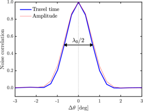
Figure 8.: Cut through the noise correlation matrix for point-to-point travel times (solid curve) and point-to-point amplitude measurements (thin-red curve) as a function of the angular distance between neighboring points. The reference observation point is kept fixed at $\theta=45.2^{\circ}$ and the target radius is $z_{t}=0.8\,\mathrm{R_{\odot}}$. The double-headed arrow indicates $\lambda_{0}/2$, where $\lambda_{0}=33.3$ Mm is the wavelength at frequency $3$ mHz.fig:noise˙corr

The model for the noise covariance matrix for travel-time and amplitude measurements was outlined in Section sec:noise_model. Figure fig:noise_corr shows a cut through the noise correlation matrix of point-to-point travel times and amplitudes. The correlation between neighboring pairs of points drops fast as a function of angular distance. For both travel-time and amplitude measurements, the correlation distance at half maximum is approximately $\lambda_{0}/2$ (see also Gizon and Birch, 2004). This justifies a posteriori why we chose points in the pupil that are separated by $\lambda_{0}/4\approx 8.3$ Mm to avoid under sampling.

4.6 Localized Sound-Speed Anomaly at $z_{0}=0.7\,\mathrm{R_{\odot}}$

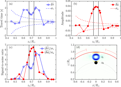
Figure 9.: (a) Deep-focusing travel-time perturbation $\overline{\delta\tau}$ (connected open circles) and (b) amplitude perturbation $\overline{\delta a}$ (connected filled circles) due to 2 % decrease in sound speed at radius $z_{0}=0.7\,\mathrm{R_{\odot}}$ given by Equation eq:target_func1. The dashed lines show the 1-$\sigma$ level of stochastic noise for an observation duration $T=$ four years. The vertical lines indicate the width of the negative sound-speed perturbation ($z_{0}\pm s$). (c) Signal-to-noise ratios for the deep-focusing travel-time and amplitude perturbations as functions of target radius. (d) Geometrical setup. The (negative) Gaussian perturbation in sound speed is indicated by the filled black circle at $\bm{r}_{0}=(x_{0},y_{0},z_{0})=(0,0,0.7\,\mathrm{R_{\odot}})$. An example deep-focusing sensitivity kernel for $\overline{\delta\tau}$ is shown for the target radius $z_{t}=0.85\,\mathrm{R_{\odot}}$.fig:d˙tau˙amp˙pupil˙target1

In order to quantify the bias and variance of the travel-time and amplitude measurements in the present deep-focusing setup, we compute the travel-time and amplitude perturbations generated by sound-speed perturbations of our choosing (forward modeling).

In this section we consider a highly localized perturbation in sound speed with a Gaussian profile centered at $\bm{r}_{0}=(x_{0},y_{0},z_{0})=(0,0,0.7\,\mathrm{R_{\odot}})$ such that

$$\frac{\delta c(\bm{r})}{c_{0}}=-A_{1}\exp\left(-\|\bm{r}-\bm{r}_{0}\|^{2}/2s^{2}\right),\ilabel{eq:target_{f}unc1}$$ (36)

where $A_{1}=0.02$. Notice that we have chosen a negative perturbation in sound speed. The parameter $s=0.03\,\mathrm{R_{\odot}}$ determines the extent of the perturbation, which is roughly of the same size as the wavelength ($\lambda_{0}\approx 0.05\,\mathrm{R_{\odot}}$). The location of the perturbation is represented by the filled black circle in Figure fig:d_tau_amp_pupil_target1(d).

Figure fig:d_tau_amp_pupil_target1(a) shows the deep-focusing travel-time measurements $[\overline{\delta\tau}]$ and the corresponding noise levels (standard deviations) for different target locations $\bm{r}_{t}=(0,0,z_{t})$, where $0.4<z_{t}/\mathrm{R_{\odot}}<1$. Due to the hollow nature of the deep-focusing travel-time kernel, the signal is weaker at the depth where the perturbation is located than in the surroundings. The bulk of the perturbation is within $|z_{0}-z_{t}|<L_{\tau}(z_{0})/2\approx 0.13\,\mathrm{R_{\odot}}$. On the other hand, a maximum signal for the amplitude measurements is obtained at the radius where the perturbation is placed (Figure fig:d_tau_amp_pupil_target1(b)) due to the concentrated sensitivity of the deep-focusing kernel for amplitude measurements (Figure fig:aveKernels(b)).

To compare the two types of measurements, travel-time versus amplitude measurements, the signal-to-noise ratios are plotted in Figure fig:d_tau_amp_pupil_target1(c). We find that the signal-to-noise ratio is higher and better localized for the amplitude measurements than for the travel-time measurements, given the highly localized perturbation in sound speed that we chose in this section.

4.7 Sound-Speed Anomaly in a Shell at Radius $r_{0}=0.7\,\mathrm{R_{\odot}}$

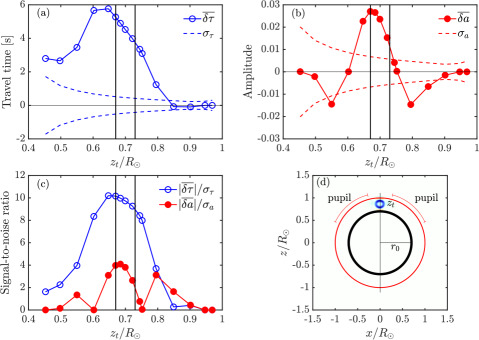
Figure 10.: (a) Deep-focusing travel-time perturbation $\overline{\delta\tau}$ and (b) amplitude perturbation $\overline{\delta a}$ due to a $0.2$ % decrease in sound speed in a thin shell at radius $r_{0}=0.7\,\mathrm{R_{\odot}}$ and defined by Equation eq:target_func2. The vertical lines indicate the width of the negative sound-speed perturbation ($r_{0}\pm s$). (c) Signal-to-noise ratios for the deep-focusing travel-time and amplitude perturbations versus target depth, for an observation duration $T=$ four years. (d) The thick black circle of thickness $2s=0.06\,\mathrm{R_{\odot}}$ indicates the location of the shell of sound-speed perturbation. The blue shades show a cut through a deep-focusing travel-time sensitivity kernel with target radius $z_{t}=0.85\,\mathrm{R_{\odot}}$.fig:d˙tau˙amp˙pupil˙target2

The search for solar-cycle changes at the bottom of the solar convection zone is a key question in helioseismology. In this section we consider a shell of perturbation in sound speed at radius $r_{0}=0.7\,\mathrm{R_{\odot}}$ with a profile given by

$$\frac{\delta c(\bm{r})}{c_{0}}=-A_{2}\exp\left(-\left(\|\bm{r}\|-r_{0}\right)^{2}/2s^{2}\right),\ilabel{eq:target_{f}unc2}$$ (37)

where $A_{2}=0.002$ and $s=0.03\,\mathrm{R_{\odot}}$. This shell of negative sound-speed perturbation is illustrated in Figure fig:d_tau_amp_pupil_target2(d). As in the previous section the radial extent of this perturbation is of the order of a wavelength.

The corresponding travel-time and amplitude perturbations, as well as the noise levels for $T=$ four years, are shown in Figures fig:d_tau_amp_pupil_target2(a) and fig:d_tau_amp_pupil_target2(b). We see that the travel-time and amplitude signals peak below $z_{t}=0.7\,\mathrm{R_{\odot}}$: the deep-focusing averaging scheme is not unbiased. For a shell-like perturbation, the signal-to-noise ratio is twice as large for the travel-time measurements as for the amplitude measurements (Figure fig:d_tau_amp_pupil_target2(c)).

5 Conclusion

sec:summary In this article we considered toy models in a uniform background medium to study the localization and noise properties of the deep-focusing time–distance technique. We considered two measurement quantities extracted from the cross-covariance function: travel times and amplitudes. The sensitivity kernels for sound speed were derived under the first Born approximation.

We computed the spatial sensitivity of travel-time and amplitude to perturbations in sound speed with respect to a uniform background medium. We find that the travel-time sensitivity to sound-speed perturbations is zero at the target location and negative in a surrounding region with diameter $L_{\tau}\approx(\lambda_{0}D)^{1/2}$, where $\lambda_{0}$ is the wavelength and $D$ is the travel distance between the points used in the deep-focusing averaging. On the other hand, the amplitude sensitivity peaks at the target location and is negative in a region with diameter $L_{a}\approx(\lambda_{0}D/2)^{1/2}$, resulting in a higher signal-to-noise ratio for small-scale perturbations. We conclude that amplitude measurements are a useful complement to travel-time measurements in local helioseismology.

In future studies, we intend to extend this work to a standard solar model using accurate computations of Green’s functions in the frequency domain. We also intend to study the capability of the deep-focusing technique to recover flows in the solar interior. Deep-focusing travel times have already been used to recover meridional circulation (e.g. Rajaguru and Antia, 2015). No significant improvement is expected from using deep-focusing amplitude measurements to recover such slowly varying flows. However, amplitude measurements should help resolve flows that vary on scales smaller than the wavelength, e.g. convective flows.

Acknowledgments

We thank Thomas L. Duvall, Aaron C. Birch, Zhi-Chao Liang, Chris S. Hanson and Kaori Nagashima for useful discussions and comments. MP is a member of the International Max Planck Research School (IMPRS) for Solar System Science at the University of Göttingen.

References

- Birch, Kosovichev, and Duvall (2004) Birch, A.C., Kosovichev, A.G., Duvall, T.L. Jr.: 2004, Sensitivity of Acoustic Wave Travel Times to Sound-Speed Perturbations in the Solar Interior. ApJ 608, 580. DOI. ADS.
- Dahlen and Baig (2002) Dahlen, F.A., Baig, A.M.: 2002, Fréchet kernels for body-wave amplitudes. Geophys. J. Int. 150, 440. DOI. ADS.
- Dalton, Hjörleifsdóttir, and Ekström (2014) Dalton, C.A., Hjörleifsdóttir, V., Ekström, G.: 2014, A comparison of approaches to the prediction of surface wave amplitude. Geophys. J. Int. 196, 386. DOI. ADS.
- Duvall (1995) Duvall, T.L. Jr.: 1995, Time-Distance Helioseismology: an Update. In: Ulrich, R.K., Rhodes, E.J. Jr., Dappen, W. (eds.) GONG 1994. Helio- and Astro-Seismology from the Earth and Space CS- 76, Astron. Soc. Pacific, 465. ADS.
- Duvall et al. (1993) Duvall, T.L. Jr., Jefferies, S.M., Harvey, J.W., Pomerantz, M.A.: 1993, Time-distance helioseismology. Nature 362, 430. DOI. ADS.
- Duvall et al. (1996) Duvall, T.L., D’Silva, S., Jefferies, S.M., Harvey, J.W., Schou, J.: 1996, Downflows under sunspots detected by helioseismic tomography. Nature 379, 235. DOI. ADS.
- Fournier et al. (2014) Fournier, D., Gizon, L., Hohage, T., Birch, A.C.: 2014, Generalization of the noise model for time-distance helioseismology. A&A 567, A137. DOI. ADS.
- Gizon (2006) Gizon, L.: 2006, Probing Convection and Solar Activity with Local Helioseismology. In: SOHO-17. 10 Years of SOHO and Beyond SP- 617, ESA, 5.1. ADS.
- Gizon and Birch (2002) Gizon, L., Birch, A.C.: 2002, Time-Distance Helioseismology: The Forward Problem for Random Distributed Sources. ApJ 571, 966. DOI. ADS.
- Gizon and Birch (2004) Gizon, L., Birch, A.C.: 2004, Time-Distance Helioseismology: Noise Estimation. ApJ 614, 472. DOI. ADS.
- Gizon and Birch (2005) Gizon, L., Birch, A.C.: 2005, Local Helioseismology. Living Rev. Sol. Phys. 2, 6. DOI. ADS.
- Gizon, Birch, and Spruit (2010) Gizon, L., Birch, A.C., Spruit, H.C.: 2010, Local Helioseismology: Three-Dimensional Imaging of the Solar Interior. ARA&A 48, 289. DOI. ADS.
- Gizon et al. (2017) Gizon, L., Barucq, H., Duruflé, M., Hanson, C.S., Leguèbe, M., Birch, A.C., Chabassier, J., Fournier, D., Hohage, T., Papini, E.: 2017, Computational helioseismology in the frequency domain: acoustic waves in axisymmetric solar models with flows. A&A 600, A35. DOI. ADS.
- Hartlep et al. (2013) Hartlep, T., Zhao, J., Kosovichev, A.G., Mansour, N.N.: 2013, Solar Wave-field Simulation for Testing Prospects of Helioseismic Measurements of Deep Meridional Flows. ApJ 762, 132. DOI. ADS.
- Hughes, Pijpers, and Thompson (2007) Hughes, S.J., Pijpers, F.P., Thompson, M.J.: 2007, Optimized data masks for focussed solar tomography: background and artificial diagnostic experiments. A&A 468, 341. DOI. ADS.
- Jensen (2001) Jensen, J.M.: 2001, Helioseismic Time–Distance Inversion. PhD thesis, University of Aarhus, Denmark.
- Langfellner, Gizon, and Birch (2015) Langfellner, J., Gizon, L., Birch, A.C.: 2015, Spatially resolved vertical vorticity in solar supergranulation using helioseismology and local correlation tracking. A&A 581, A67. DOI. ADS.
- Liang et al. (2013) Liang, Z.-C., Gizon, L., Schunker, H., Philippe, T.: 2013, Helioseismology of sunspots: defocusing, folding, and healing of wavefronts. A&A 558, A129. DOI. ADS.
- Moradi and Hanasoge (2010) Moradi, H., Hanasoge, S.M.: 2010, Deep-Focus Diagnostics of Sunspot Structure. Astrophysics and Space Science Proceedings 19, 378. DOI. ADS.
- Nagashima et al. (2017) Nagashima, K., Fournier, D., Birch, A.C., Gizon, L.: 2017, The amplitude of the cross-covariance function of solar oscillations as a diagnostic tool for wave attenuation and geometrical spreading. A&A 599, A111. DOI. ADS.
- Nolet, Dahlen, and Montelli (2005) Nolet, G., Dahlen, F.A., Montelli, R.: 2005, Traveltimes and amplitudes of seismic waves: A re-assessment. Washington DC American Geophysical Union Geophysical Monograph Series 157, 37. DOI. ADS.
- Rajaguru and Antia (2015) Rajaguru, S.P., Antia, H.M.: 2015, Meridional Circulation in the Solar Convection Zone: Time-Distance Helioseismic Inferences from Four Years of HMI/SDO Observations. ApJ 813, 114. DOI. ADS.
- Tong et al. (1998) Tong, J., Dahlen, F.A., Nolet, G., Marquering, H.: 1998, Diffraction effects upon finite-frequency travel times: A simple 2-D example. Geophys. Res. Lett. 25, 1983. DOI. ADS.
- Zhao et al. (2013) Zhao, J., Bogart, R.S., Kosovichev, A.G., Duvall, T.L. Jr., Hartlep, T.: 2013, Detection of Equatorward Meridional Flow and Evidence of Double-cell Meridional Circulation inside the Sun. ApJ 774, L29. DOI. ADS.