Accelerated Optimization in the PDE Framework: Formulations for the Manifold of Diffeomorphisms

Abstract

We consider the problem of optimization of cost functionals on the infinite-dimensional manifold of diffeomorphisms. We present a new class of optimization methods, valid for any optimization problem setup on the space of diffeomorphisms by generalizing Nesterov accelerated optimization to the manifold of diffeomorphisms. While our framework is general for infinite dimensional manifolds, we specifically treat the case of diffeomorphisms, motivated by optical flow problems in computer vision. This is accomplished by building on a recent variational approach to a general class of accelerated optimization methods by Wibisono, Wilson and Jordan [1], which applies in finite dimensions. We generalize that approach to infinite dimensional manifolds. We derive the surprisingly simple continuum evolution equations, which are partial differential equations, for accelerated gradient descent, and relate it to simple mechanical principles from fluid mechanics. Our approach has natural connections to the optimal mass transport problem. This is because one can think of our approach as an evolution of an infinite number of particles endowed with mass (represented with a mass density) that moves in an energy landscape. The mass evolves with the optimization variable, and endows the particles with dynamics. This is different than the finite dimensional case where only a single particle moves and hence the dynamics does not depend on the mass. We derive the theory, compute the PDEs for accelerated optimization, and illustrate the behavior of these new accelerated optimization schemes.

I Introduction

Accelerated optimization methods have gained wide applicability within the machine learning and optimization communities (e.g., [2, 3, 4, 5, 6, 7, 8, 9, 10, 11, 12]). They are known for leading to optimal convergence rates among schemes that use only gradient (first order) information in the convex case. In the non-convex case, they appear to provide robustness to shallow local minima. The intuitive idea is that by considering a particle with mass that moves in an energy landscape, the particle will gain momentum and surpass shallow local minimum and settle in in more wider, deeper local extrema in the energy landscape. This property has made them (in conjunction with stochastic search algorithms) particularly useful in machine learning, especially in the training of deep networks, where the optimization is a non-convex problem that is riddled with local minima. These methods have so far have only been used in optimization problems that are defined in finite dimensions. In this paper, we consider the generalization of these methods to infinite dimensional manifolds. We are motivated by applications in computer vision, in particular, segmentation, 3D reconstruction, and optical flow. In these problems, the optimization is over infinite dimensional geometric quantities (e.g., curves, surfaces, mappings), and so the problems are formulated on infinite dimensional manifolds. Recently there has been interest within the machine learning community in optimization on finite dimensional manifolds, such as matrix groups, e.g., [13, 14, 15], which have particular structure not available on infinite dimensional manifolds that we consider here.

Recent work [1] has shown that the continuum limit of accelerated methods, which are discrete optimization algorithms, may be formulated with variational principles. This allows one to derive the continuum limit of accelerated optimization methods (Nesterov’s optimization method [12] and others) as an optimization problem on descent paths. The resulting optimal continuum path is defined by an ODE, which when discretized appropriately yields Nesterov’s method and other accelerated optimization schemes. The optimization problem on paths is an action integral, which integrates the Bregman Lagrangian. The Bregman Lagrangian is a time-explicit Lagrangian (from physics) that consists of kinetic and potential energies. The kinetic energy is defined using the Bregman divergence (see Section II-B); it is designed for finite step sizes, and thus differs from classical action integrals in physics [16, 17]. The potential energy is the cost function that is to be optimized.

We build on the approach of [1] by formulating accelerated optimization with an action integral, but we generalize that approach to infinite dimensional manifolds. Our approach is general for infinite dimensional manifolds, but we illustrate the idea here for the case of the infinite dimensional manifold of diffeomorphisms of $\mathbb{R}^{n}$ (the case of the manifold of curves has been recently formulated by the authors [18]). To do this, we abandon the Bregman Lagrangian framework in [1] since that assumes that the variable over which one optimizes is embedded in $\mathbb{R}^{n}$.

Instead, we adopt the classical formulation of action integrals in physics [16, 17], which is already general enough to deal with manifolds, and kinetic energies that are defined through general Riemannian metrics rather than a traditional Euclidean metric, thus by-passing the need for the use of Bregman distances. Our approach requires consideration of additional technicalities beyond that of [1] and classical physics. Namely, in finite dimensions in $\mathbb{R}^{n}$, one can think of accelerated optimization as a single particle with mass moving in an energy landscape. Since only a single particle moves, mass is a fixed constant that does not impact the dynamics of the particle. However, in infinite dimensions, one can instead think of an infinite number of particles each moving, and these masses of particles is better modeled with a mass density. In the case of the manifold of diffeomorphisms of $\mathbb{R}^{n}$ this mass density exists in $\mathbb{R}^{n}$. As the diffeomorphism evolves to optimize the cost functional, it deforms $\mathbb{R}^{n}$ and redistributes the mass, and so the density changes in time. Since the mass density defines the kinetic energy and the stationary action path depends on the kinetic energy, the dynamics of the evolution to minimize the cost functional depends on the way that mass is distributed in $\mathbb{R}^{n}$. Therefore, in the infinite dimensional case, one also needs to optimize and account for the mass density, which cannot be neglected. Further, our approach, due to the infinite dimensional nature, has evolution equations that are PDEs rather than ODEs in [1]. Finally, the discretization of the resulting PDEs requires the use of entropy schemes [19] since our evolution equations are defined as viscosity solutions of PDEs, required to treat shocks and rarefaction fans. These phenomena appear not to be present in the finite dimensional case.

I-A Related Work

I-A1 Sobolev Optimization

Our work is motivated by Sobolev gradient descent approaches [20, 21, 22, 23, 24, 25, 26, 27, 28, 29] for optimization problems on manifolds, which have been used for segmentation and optical flow problems. These approaches are general in that they apply to non-convex problems, and they are derived by computing the gradient of a cost functional with respect to a Sobolev metric rather than an $L^{2}$ metric typically assumed in variational optimization problems. The resulting gradient flows have been demonstrated to yield coarse-to-fine evolutions, where the optimization automatically transitions from coarse to successively finer scale deformations. This makes the optimization robust to local minimizers that plague $L^{2}$ gradient descents. We should point out that the Sobolev metric is used beyond optimization problems and have been used extensively in shape analysis (e.g., [30, 31, 32, 33]). While such gradient descents are robust to local minimizers, computing them in general involves an expensive computation of an inverse differential operator at each iteration of the gradient descent. In the case of optimization problems on curves and a very particular form of a Sobolev metric this can be made computationally fast [23], but the idea does not generalize beyond curves. In this work, we aim to obtain robustness properties of Sobolev gradient flows, but without the expensive computation of inverse operators. Our accelerated approach involves averaging the gradient across time in the descent process, rather than an averaging across space in the Sobolev case. Despite our goal of avoiding Sobolev gradients for computational speed, we should mention that our framework is general to allow one to consider accelerated Sobolev gradient descents (although we do not demonstrate it here), where there is averaging in both space and time. This can be accomplished by changing the definition of kinetic energy in our approach. This could be useful in applications where added robustness is needed but speed is not a critical factor.

I-A2 Optimal Mass Transport

Our work relates to the literature on the problem of optimal mass transportion (e.g., [34, 35, 36]), especially the formulation of the problem in [37]. The modern formulation of the problem, called the Monge-Kantorovich problem, is as follows. One is given two probability densities $\rho_{0},\rho_{1}$ in $\mathbb{R}^{n}$, and the goal is to compute a transformation $M:\mathbb{R}^{n}\to\mathbb{R}^{n}$ so that the pushforward of $\rho_{0}$ by $M$ results in $\rho_{1}$ such that $M$ has minimal cost. The cost is defined as the average Euclidean norm of displacement: $\int_{\mathbb{R}^{n}}|M(x)-x|^{p}\rho_{0}(x)\,\mathrm{d}x$ where $p\geq 1$. The value of the minimum cost is a distance (called the $L^{p}$ Wasserstein distance) on the space of probability measures. In the case that $p=2$, [37] has shown that mass transport can be formulated as a fluid mechanics problem. In particular, the Wasserstein distance can be formulated as a distance arising from a Riemannian metric on the space of probability densities. The cost can be shown equivalent to the minimum Riemannian path length on the space of probability densities, with the initial and final points on the path being the two densities $\rho_{0},\rho_{1}$. The tangent space is defined to be velocities of the density that infinitesimally displace the density. The Riemannian metric is just the kinetic energy of the mass distribution as it is displaced by the velocity, given by $\int_{\mathbb{R}^{n}}\frac{1}{2}\rho(x)|v(x)|^{2}\,\mathrm{d}x$. Therefore, optimal mass transport computes an optimal path on densities that minimizes the integral of kinetic energy along the path.

In our work, we seek to minimize a potential on the space of diffeomorphisms, with the use of acceleration. We can imagine that each diffeomorphism is associated with a point on a manifold, and the goal is to move to the bottom of the potential well. To do so, we associate a mass density in $\mathbb{R}^{n}$, which as we optimize the potential, moves in $\mathbb{R}^{n}$ via a push-forward of the evolving diffeomorphism. We regard this evolution as a path in the space of diffeomorphisms that arises from an action integral, where the action is the difference of the kinetic and potential energies. The kinetic energy that we choose, purely to endow the diffeomorphism with acceleration, is the same one used in the fluid mechanics formulation of optimal mass transportation for $p=2$. We have chosen this kinetic energy for simplicity to illustrate our method, but we envision a variety of kinetic energies can be defined to introduce different dynamics. The main difference of our approach to the fluid mechanics formulation of mass transport is in the fact that we do not minimize just the path integral of the kinetic energy, but rather we derive our method by computing stationary paths of the path integral of kinetic minus potential energies. Since diffeomorphisms are generated by smooth velocity fields, we equivalently optimize over velocities. We also optimize over the mass distribution. Thus, the main difference between the fluid mechanics formulations of $L^{2}$ mass transport and our approach is the potential on diffeomorphisms, which is used to define the action integral.

I-A3 Diffeomorphic Image Registration

Our work relates to the literature on diffeomorphic image registration [21, 38], where the goal, similar to ours, is to compute a registration between two images as a diffeomorphism. There a diffeomorphism is generated by a path of smooth velocity fields integrated over the path. Rather than formulating an optimization problem directly on the diffeomorphism, the optimization problem is formed on a path of velocity fields. The optimization problem is to minimize $\int_{0}^{1}\|v\|^{2}\,\mathrm{d}t$ where $v$ is a time varying vector field, $\|\cdot\|$ is a norm on velocity fields, and the optimization is subject to the constraint that the mapping $\phi$ maps one image to the other, i.e., $I_{1}=I_{0}\circ\phi^{-1}$. The minimization can be considered the minimization of an action integral where the action contains only a kinetic energy. The norm is chosen to be a Sobolev norm to ensure that the generated diffeomorphism (by integrating the velocity fields over time) is smooth. The optimization problem is solved in [21] by a Sobolev gradient descent on the space of paths. The resulting path is a geodesic with Riemannian metric given by the Sobolev metric $\|v\|$. In [38], it is shown these geodesics can be computed by integrating a forward evolution equation, determined from the conservation of momentum, with an initial velocity.

Our framework instead uses accelerated gradient descent. Like [21, 38], it is derived from an action integral, but the action has both a kinetic energy and a potential energy, which is the objective functional that is to be optimized. In this current work, our kinetic energy arises naturally from physics rather than a Sobolev norm. One of our motivations in this work is to get regularizing effects of Sobolev norms without using Sobolev norms, since that requires inverting differential operators in the optimization, which is computationally expensive. Our kinetic energy is an $L^{2}$ metric weighted by mass. Our method has acceleration, rather than zero acceleration in [21, 38], and this is obtained by endowing a diffeomorphism with mass, which is a mass density in $\mathbb{R}^{n}$. This mass allows for the kinetic energy to endow the optimization with dynamics. Our optimization is obtained as the stationary conditions of the action with respect to both velocity and mass density. The latter links our approach to optimal mass transport, described earlier. Our physically motivated kinetic energy and in particular the mass consideration allows us to generate diffeomorphisms without the use fo Sobolev norms. We also avoid the inversion of differential operators.

I-A4 Optical Flow

Although our framework is general in solving any optimization on infinite dimensional manifolds, we demonstrate the framework for optimization of diffeomorphisms and specifically for optical flow problems formulated as variational problems in computer vision (e.g., [39, 40, 41, 42, 43, 44, 45]). Optical flow, i.e., determining pixel-wise correspondence between images, is a fundamental problem in computer vision that remains a challenge to solve, mainly because optical flow is a non-convex optimization problem, and thus few methods exist to optimize such problems. Optical flow was first formulated as a variational problem in [39], which consisted of a data fidelity term and regularization favoring smooth optical flow. Since the problem is non-convex, approaches to solve this problem typically involve the assumption of small displacement between frames, so a linearization of the data fidelity term can be performed, and this results in a problem in which the global optimum of [39] can be solved via the solution of a linear PDE. Although standard gradient descent could be used on the non-linearized problem, it is numerically sensitive, extremely computationally costly, and does not produce meaningful results unless coupled with the strategy described next. Large displacements are treated with two strategies: iterative warping and image pyramids. Iterative warping involves iteration of the linearization around the current accumulated optical flow. By use of image pyramids, a large displacement is converted to a smaller displacement in the downsampled images. While this strategy is successful in many cases, there are also many problems associated with linearization and pyramids, such as computing optical flow of thin structures that undergo large displacements. This basic strategy of linearization, iterative warping and image pyramids have been the dominant approach to many variational optical flow models (e.g., [39, 40, 41, 42, 43]), regardless of the regularization that is used (e.g., use of robust norms, total variation, non-local norms, etc). In [42], the linearized problem with TV regularization has been formulated as a convex optimization problem, in which a primal-dual algorithm can be used. In [29] linearization is avoided and rather a gradient descent with respect to a Sobolev metric is computed, and is shown to have a automatic coarse-to-fine optimization behavior. Despite these works, most optical flow algorithms involve simplification of the problem into a linear problem. In this work, we construct accelerated gradient descent algorithms that are applicable to any variational optical flow algorithm in which we avoid the linearization step and aim to obtain a better optimizer. For illustration, we consider here the case of optical flow modeled as a global diffeomorphism, but in principle this can be generalized to piecewise diffeomorphisms as in [45]. Since diffeomorphisms do not form a linear space, rather a infinite-dimensional manifold, we generalize accelerated optimization to that space.

II Background for Accelerated Optimization on Manifolds

II-A Manifolds and Mechanics

We briefly summarize the key facts in classical mechanics that are the basis for our accelerated optimization method on manifolds.

II-A1 Differential Geometry

We review differential geometry (from [46]), as this will be needed to derive our accelerated optimization scheme on the manifold of diffeomorphisms. First a manifold $M$ is a space in which every point $p\in M$ has a (invertible) mapping $f_{p}$ from a neighborhood of $p$ to a model space that is a linear normed vector space, and has an additional compatibility condition that if the neighborhoods for $p$ and $q$ overlap then the mapping $f_{p}\circ f_{q}^{-1}$ is differentiable. Intuitively, a manifold is a space that locally appears flat. The model space may be finite or infinite dimensional when the model spaces are finite or infinite dimensional, respectively. In the latter case the manifold is referred to as an infinite dimensional manifold and in the former case a finite dimensional manifold. The space of diffeomorphisms of $\mathbb{R}^{n}$, the space of interest in this paper, is an infinite dimensional manifold. The tangent space at a point $p\in M$ is the equivalence class, $[\gamma]$, of curves $\gamma:[0,1]\to M$ under the equivalence that $\gamma(0)=p$ and $(f_{p}\circ\gamma)^{\prime}(0)$ are the same for each curve $\gamma\in[\gamma]$. Intuitively, these are the set of possible directions of movement at the point $p$ on the manifold. The tangent bundle, denoted $TM$, is $TM=\{(p,v)\,:\,p\in M,v\in T_{p}M\}$, i.e., the space formed from the collection of all points and tangent spaces.

In this paper, we will assume additional structure on the manifold, namely, that an inner product (called the metric) exists on each tangent space $T_{p}M$. Such a manifold is called a Riemannian manifold. A Riemannian manifold allows one to formally define the lengths of curves $\gamma:[-1,1]\to M$ on the manifold. This allows one to construct paths of critical length, called geodesics, a generalization of a path on constant velocity on the manifold. Note that while existence of geodesics is guaranteed on finite dimensional manifolds, in the infinite dimensional case, there is no such guarantee. The Riemannian metric also allows one to define gradients of functions $g:M\to\mathbb{R}$ defined on the manifold: the gradient $\nabla g(p)\in T_{p}M$ is defined to be the vector that satisfies $\frac{\,\mathrm{d}{}}{\,\mathrm{d}{\varepsilon}}\left.g(\gamma(\varepsilon))\right|_{\varepsilon=0}=\left<{\nabla g(p)},{\gamma^{\prime}(0)}\right>$, where $\gamma(0)=p$, the left hand side is the directional derivative and the right hand side is the inner product from the Riemannian structure.

II-A2 Mechanics on Manifolds

We now briefly review some of the formalism of classical mechanics on manifolds that will be used in this paper. The material is from [16, 17]. The subject of mechanics describes the principles governing the evolution of a particle that moves on a manifold $M$. The equations governing a particle are Newton’s laws. There are two viewpoints in mechanics, namely the Lagrangian and Hamiltonian viewpoints, which formulate more general principles to derive Newton’s equations. In this paper, we use the Lagrangian formulation to derive equations of motion for accelerated optimization on the manifold of diffeomorphisms. Lagrangian mechanics obtains equations of motion through variational principles, which makes it easier to generalize Newton’s laws beyond simple particle systems in $\mathbb{R}^{3}$, especially to the case of manifolds. In Lagrangian mechanics, we start with a function $L:TM\to\mathbb{R}$, called the Lagrangian, from the tangent bundle to the reals. Here we assume that $M$ is a Riemannian manifold. One says that a curve $\gamma:[-1,1]\to M$ is a motion in a Lagrangian system with Lagrangian $L$ if it is an extremal of $A=\int L(\gamma(t),\dot{\gamma}(t))\,\mathrm{d}t$. The previous integral is called an action integral. Hamilton’s principle of stationary action states that the motion in the Lagrangian system satisfies the condition that $\delta A=0$, where $\delta$ denotes the variation, for all variations of $A$ induced by variations of the path $\gamma$ that keep endpoints fixed. The variation is defined as $\delta A:=\frac{\,\mathrm{d}{}}{\,\mathrm{d}{s}}\left.A(\tilde{\gamma}(t,s))\right|_{s=0}$ where $\tilde{\gamma}:[-1,1]^{2}\to M$ is a smooth family of curves (a variation of $\gamma$) on the manifold such that $\tilde{\gamma}(t,0)=\gamma(t)$. The stationary conditions give rise to what is known as Lagrange’s equations. A natural Lagrangian has the special form $L=T-U$ where $T:TM\to\mathbb{R}^{+}$ is the kinetic energy and $U:M\to\mathbb{R}$ is the potential energy. The kinetic energy is defined as $T(v)=\frac{1}{2}\left<{v},{v}\right>$ where $\left<{\cdot},{\cdot}\right>$ is the inner product from the Riemannian structure. In the case that one has a particle system in $\mathbb{R}^{3}$, i.e., a collection of particles with masses $m_{i}$, in a natural Lagrangian system, one can show that Hamilton’s principle of stationary action is equivalent to Newton’s law of motion, i.e., that $\frac{\,\mathrm{d}{}}{\,\mathrm{d}{t}}(m_{i}\dot{r}_{i})=-\frac{\partial{U}}{\partial{r_{i}}}$ where $r_{i}$ is the trajectory of the $i^{\text{th}}$ particle, and $\dot{r}_{i}$ is the velocity. This states that mass times acceleration is the force, which is given by minus the derivative of the potential in a conservative system. Thus, Hamilton’s principle is more general and allows us to more easily derive equations of motion for more general systems, in particular those on manifolds.

In this paper, we will consider Lagrangian non-autonomous systems where the Lagrangian is also an explicit function of time $t$, i.e., $L:TM\times\mathbb{R}\to\mathbb{R}$. In particular, the kinetic and potential energies can both be explicit functions of time: $T:TM\times\mathbb{R}\to\mathbb{R}$ and $U:M\times\mathbb{R}\to\mathbb{R}$. Autonomous systems have an energy conservation property and do not converge; for instance, one can think of a moving pendulum with no friction, which oscillates forever. Since the objective in this paper is to minimize an objective functional, we want the system to eventually converge and Lagrangian non-autonomous systems allow for this possibility. For completness, we present some basic facts of the Hamiltonian perspective to elaborate on the previous point, although we do not use this in the present paper. The generalization of total energy is the Hamiltonian, defined as the Legendre transform of the Lagrangian: $H(p,q,t)=\left<{p},{\dot{q}}\right>-L(q,\dot{q},t)$ where $p=\frac{\,\mathrm{d}{L}}{\,\mathrm{d}{\dot{q}}}$ is the fiber derivative of $L$ with respect to $\dot{q}$, i.e., $\frac{\,\mathrm{d}{L}}{\,\mathrm{d}{\dot{q}}}\cdot w=\frac{\,\mathrm{d}{}}{\,\mathrm{d}{\varepsilon}}\left.L(q,\dot{q}+\varepsilon w)\right|_{\varepsilon=0}$. From the Hamiltonian, one can also obtain a system of equations describing motion on the manifold. It can be shown that if $L=T-U$ then $H=T+U$ and more generally, $\frac{\,\mathrm{d}{H}}{\,\mathrm{d}{t}}=-\frac{\partial{L}}{\partial{t}}$ along the stationary path of the action. Thus, if the Lagrangian is natural and autonomous, the total energy is preserved, otherwise energy could be dissipated based on the partial of the Lagrangian with respect to $t$.

II-B Variational Approach to Accelerated Optimization in Finite Dimensional Vector Spaces

Accelerated gradient optimization can be motivated by the desire to make an ordinary gradient descent algorithm 1) more robust to noise and local minimizers, and 2) speed-up the convergence while only using first order (gradient) information. For instance, if one computes a noisy gradient due imperfections in obtaining an accurate gradient, a simple heuristic to make the algorithm more robust is to compute a running average of the gradient over iterations, and use that as the search direction. This also has the advantage, for instance in speeding up optimization in narrow shallow valleys. Gradient descent (with finite step sizes) would bounce back and forth across the valley and slowly descend down, but averaging the gradient could cancel the component across the valley and more quickly optimize the function. Strategic dynamically changing weights on previous gradients can boost the descent rate. Nesterov put forth the following famous scheme [12] which attains an optimal rate of order $\frac{1}{t^{2}}$ in the case of a smooth, convex cost function $f(x)$:

$$y_{k+1}=x_{k}-\frac{1}{\beta}\nabla f(x_{k}),\qquad x_{k+1}=(1-\gamma_{k})y_{k+1}+\gamma_{k}y_{k},\qquad\gamma_{k}=\frac{1-\lambda_{k}}{\lambda_{k}+1},\qquad\lambda_{k}=\frac{1+\sqrt{1+4\lambda_{k-1}^{2}}}{2}$$

where $x_{k}$ is the $k$-th iterate of the algorithm, $y_{k}$ is an intermediate sequence, and $\gamma_{k}$ are dynamically updated weights.

Recently [1] presented a variational generalization of Nesterov’s [12] and other accelerated gradient descent schemes in $\mathbb{R}^{n}$ based on the Bregman divergence of a convex distance generating function $h$:

$$d(y,x)=h(y)-h(x)-\nabla h(x)\cdot(y-x)$$ (1)

and careful discretization of the Euler-Lagrange equations for the time integral of the following Bregman Lagrangian

$$L(X,V,t)=e^{a(t)+\gamma(t)}\left[d(X+e^{-a(t)}V,X)-e^{b(t)}U(X)\right]$$

where the potential energy $U$ represents the cost to be minimized. In the Euclidean case where $h(x)=\frac{1}{2}|x|^{2}$ gives $d(y,x)=\frac{1}{2}|y-x|^{2}$, this simplifies to

$$L=e^{\gamma(t)}\left[e^{-a(t)}\frac{1}{2}|V|^{2}-e^{a(t)+b(t)}U(X)\right]$$

where $T=\frac{1}{2}|V|^{2}$ is the kinetic energy of a unit mass particle in $\mathbb{R}^{n}$. Nesterov’s methods [12, 47, 48, 11, 49, 10] belong to a subfamily of Bregman Lagrangians with the following choice of parameters (indexed by $k>0$)

$$a=\log k-\log t,\qquad b=k\,\log t+\log\lambda,\qquad\gamma=k\,\log t$$

which, in the Euclidean case, yields a non-autonomous Lagrangian as follows:

$$L=\frac{t^{k+1}}{k}\left(T-\lambda k^{2}t^{k-2}U\right)$$ (2)

In the case of $k=2$, for example, the stationary conditions of the integral of this time-explicit action yield the continuum limit of Nesterov’s accelerated mirror descent [10] derived in both [50, 8].

Since the Bregman Lagrangian assumes that the underlying manifold is a subset of $\mathbb{R}^{n}$ (in order to define the Bregman distance), which many manifolds do not have - for instance the manifold of diffeomorphisms that we consider in this paper, we instead use the original classical mechanics formulation, which already provides a formalism for considering general metrics though the Riemannian distance, although not equivalent to the Bregman distance.

III Accelerated Optimization for Diffeomorphisms

In this section, we use the mechanics of particles on manifolds developed in the previous section, and apply it to the case of the infinite-dimensional manifold of diffeomorphisms in $\mathbb{R}^{n}$ for general $n$. This allows us to generalize accelerated optimization to infinite dimensional manifolds. Diffeomorphisms are smooth mappings $\phi:\mathbb{R}^{n}\to\mathbb{R}^{n}$ whose inverse exists and is also smooth. Diffeomorphisms form a group under composition. The inverse operator on the group is defined as the inverse of the function, i.e., $\phi^{-1}(\phi(x))=x$. Here smoothness will mean that two derivatives of the mapping exist. The group of diffeomorphisms will be denoted $\mbox{Diff}(\mathbb{R}^{n})$. Diffeomorphisms relate to image registration and optical flow, where the mappings between two images are often modeled as diffeomorphisms. Recovering diffeomorphisms from two images will be formulated as an optimization problem $U(\phi)$ where $U$ will correspond to the potential energy. Note we avoid calling $U$ the energy as is customary in computer vision literature, because for us the energy will refer to the total mechanical energy (i.e., the sum of the kinetic and potential energies). We do not make any assumptions on the particular form of the potential in this section, as our goal is to be able to accelerate any optimization problem for diffeomorphisms, given that one can compute a gradient of the potential. The formulation here allows any of the numerous cost functionals developed over the past three decades for image registration to be accelerated.

In the first sub-section, we give the formulation and evolution equations for the case of acceleration without energy dissipation (Hamiltonian is conserved), since most of the calculations are relevant for the case of energy dissipation, which is needed for the evolution to converge to a diffeomorphism. In the second sub-section, we formulate and compute the evolution equations for the energy dissipation case, which generalizes Nesterov’s method to the infinite dimensional manifold of diffeomorphisms. Finally, in the last sub-section we give an example potential and its gradient calculation for a standard image registration or optical flow problem.

III-A Acceleration Without Energy Dissipation

III-A1 Formulation of the Action Integral

Since the potential energy $U$ is assumed given, in order to formulate the action integral in the non-dissipative case, we need to define kinetic energy $T$ on the space of diffeomorphisms. Since diffeomorphisms form a manifold, we can apply the the results in the previous section and note that the kinetic energy will be defined on the tangent space to $\mbox{Diff}(\mathbb{R}^{n})$ at a particular diffeomorphism $\phi$. This will be denoted $T_{\phi}\mbox{Diff}(\mathbb{R}^{n})$. The tangent space at $\phi$ can be roughly thought of as the set of local perturbations $v$ of $\phi$ given for all $\varepsilon$ small that perserve the diffeomorphism property, i.e., $\phi+\varepsilon v$ is a diffeomorphism. One can show that the tangent space is given by

$$T_{\phi}\mbox{Diff}(\mathbb{R}^{n})=\{v:\phi(\mathbb{R}^{n})\to\mathbb{R}^{n}\,:\,v\mbox{ is smooth }\}.$$ (3)

In the above, since $\phi$ is a diffeomorphism, we have that $\phi(\mathbb{R}^{n})=\mathbb{R}^{n}$. However, we write $v:\phi(\mathbb{R}^{n})\to\mathbb{R}^{n}$ to emphasize that the velocity fields in the tangent space are defined on the range of $\phi$, so that $v$ is interpreted as a Eulerian velocity. By definition of the tangent space, an infinitesimal perturbation of $\phi$ by a tangent vector, given by $\phi+\varepsilon v$, will be a diffeomorphism for $\varepsilon$ sufficiently small. Note that the previous operation of addition is defined as follows:

$$(\phi+\varepsilon v)(x)=\phi(x)+\varepsilon v(\phi(x)).$$

The tangent space is a set of smooth vector fields on $\phi(\mathbb{R}^{n})$ in which the vector field at each point $\phi(x)$, displaces $\phi(x)$ infinitesimally by $v(\phi(x))$ to form another diffeomorphism.

We note a classical result from [51], which will be of utmost importance in our derivation of accelerated optimization on $\mbox{Diff}(\mathbb{R}^{n})$. The result is that any (orientable) diffeomorphism may be generated by integrating a time-varying smooth vector field over time, i.e.,

$$\partial_{t}\phi_{t}(x)=v_{t}(\phi_{t}(x)),\quad x\in\mathbb{R}^{n},$$ (4)

where $\partial_{t}$ denotes partial derivative with respect to $t$, $\phi_{t}$ denotes a time varying family of diffeomorphisms evaluated at the time $t$, and $v_{t}$ is a time varying collection of vector fields evaluated at time $t$. The path $t\to\phi_{t}(x)$ for a fixed $x$ represents a trajectory of a particle starting at $x$ and flowing according to the velocity field.

The space on which the kinetic energy is defined is now clear, but one more ingredient is needed before we can define the kinetic energy. Any accelerated method will need a notion of mass, otherwise acceleration is not possible, e.g., a mass-less ball will not accelerate. We generalize the concept of mass to the infinite dimensional manifold of diffeomorphisms, where there are infinitely more possibilities than a single particle in the finite dimensional case considered by [1]. There optimization is done on a finite dimensional space, the space of a single particle, and the possible choices of mass are just different fixed constants. The choice of the constant, given the particle’s mass remains fixed, is irrelevant to the final evolution. This is different in than the case of diffeomorphisms. Here we imagine that an infinite number of particles densely distributed in $\mathbb{R}^{n}$ with mass exist and are displaced by the velocity field $v$ at every point. Since the particles are densely distributed, it is natural to represent the mass of all particles with a mass density $\rho:\mathbb{R}^{n}\to\mathbb{R}$, similar to a fluid at a fixed time instant. The density $\rho$ is defined as mass divided by volume as the volume shrinks. During the evolution to optimize the potential $U$, the particles are displaced continuously and thus the density of these particles will in general change over time. Note the density will change even if the density at the start is constant except in the case of full translation motion (when $v$ is spatially constant). The latter case is not general enough, as we want to capture general diffeomorphisms. We will assume that the system of particles in $\mathbb{R}^{n}$ is closed and so we impose a mass preservation constraint, i.e.,

$$\int_{\mathbb{R}^{n}}\rho(x)\,\mathrm{d}x=1,$$ (5)

where we assume the total mass is one without loss of generality. Note that the evolution of a time varying density $\rho_{t}$ as it is deformed in time by a time varying velocity is given by the continuity equation, which is a local form of the conservation of mass given by (5). The continuity equation is defined by the partial differential equation

$$\partial_{t}\rho(x)+\mbox{div}\left({\rho(x)v(x)}\right)=0,\quad x\in\mathbb{R}^{n}$$ (6)

where $\mbox{div}\left({}\right)$ denotes the divergence operator acting on a vector field and is $\mbox{div}\left({F}\right)=\sum_{i=}^{n}\partial_{x_{i}}F^{i}$ where $\partial_{x_{i}}$ is the partial with respect to the $i^{\text{th}}$ coordinate and $F^{i}$ is the $i^{\text{th}}$ component of the vector field. We will assume that the mass distribution dies down to zero outside a compact set so as to avoid boundary considerations in our derivations.

We now have the two ingredients, namely the tangent vectors to $\mbox{Diff}(\mathbb{R}^{n})$ and the concept of mass, which allows us to define a natural physical extension of the kinetic energy to the case of an infinite mass distribution. We present one possible kinetic energy to illustrate the idea of accelerated optimization, but this is by no means the only definition of kinetic energy. We envision this to be part of the design process in which one could get a multitude of various different accelerated optimization schemes by defining different kinetic energies. Our definition of kinetic energy is just the kinetic energy arising from fluid mechanics:

$$T(v)=\int_{\phi(\mathbb{R}^{n})}\frac{1}{2}\rho(x)|v(x)|^{2}\,\mathrm{d}x,$$ (7)

which is just the integration of single particle’s kinetic energy $\frac{1}{2}m|v|^{2}$ and matches the definition of the kinetic energy of a sum of particles in elementary physics. Note that the kinetic energy is just one-half times the norm squared for the norm arising from the Riemannian metric [16], i.e., an inner product on the tangent space of $\mbox{Diff}(\mathbb{R}^{n})$. The Riemannian metric is given by $\left<{v_{1}},{v_{2}}\right>=\int_{\mathbb{R}^{n}}\rho(x)v_{1}(x)\cdot v_{2}(x)\,\mathrm{d}x$, which is just a weighted $\mathbb{L}^{2}$ inner product.

We are now ready to define the action integral for the case of $\mbox{Diff}(\mathbb{R}^{n})$, which is defined on paths of diffeomorphisms. A path of diffeomorphisms is $\phi:[0,\infty)\times\mathbb{R}^{n}\to\mathbb{R}^{n}$ and we will denote the diffeomorphism at time $t$ along this path as $\phi_{t}$. Since diffeomorphisms are generated by velocity fields, we may equivalently define the action in terms of paths of velocity fields. A path of velocity fields is given by $v:[0,\infty)\times\mathbb{R}^{n}\to\mathbb{R}^{n}$, and the velocity at time $t$ along the path is denoted $v_{t}$. Notice that the action requires a kinetic energy and the kinetic energy is dependent on the mass density. Thus, a path of densities $\rho:[0,\infty)\times\mathbb{R}^{n}\to\mathbb{R}^{+}$ is required, which represents the mass distribution of the particles in $\mathbb{R}^{n}$ as they are deformed along time by the velocity field $v_{t}$. This path of densities is subject to the continuity equation. With this, the action integral is then

$$A=\int\left[T(v_{t})-U(\phi_{t})\right]\,\mathrm{d}t,$$ (8)

where the integral is over time, and we do not specify the limits of integration as it is irrelevant as the endpoints will be fixed and the action will be thus independent of the limits. Note that the action is implicitly a function of three paths, i.e., $v_{t},\phi_{t}$ and $\rho_{t}$. Further, these paths are not independent of each other as $\phi_{t}$ depends on $v_{t}$ through the generator relation (4), and $\rho_{t}$ depends on $v_{t}$ through the continuity equation (6).

III-A2 Stationary Conditions for the Action

We now derive the stationary conditions for the action integral (8), and thus the evolution equation for a path of diffeomorphisms, which is Hamilton’s principle of stationary action, equivalent to a generalization of Newton’s laws of motion extended to diffeomorphisms. As discussed earlier, we would like to find the stationary conditions for the action integral (8), defined on the path $\phi_{t}$, under the conditions that it is generated by a path of smooth velocity fields $v_{t}$, which is also coupled with the mass density $\rho_{t}$.

We treat the computation of the stationary conditions of the action as a constrained optimization problem with respect to the two aforementioned constraints. To do this, it is easier to formulate the action in terms of the path of the inverse diffeomorphisms $\phi^{-1}_{t}$, which we will call $\psi_{t}$. This is because the non-linear PDE constraint (4) can be equivalently reformulated as the following linear transport PDE in the inverse mappings:

$$\partial_{t}\psi_{t}(x)+[D\psi_{t}(x)]v_{t}(x)=0,\quad x\in\mathbb{R}^{n}$$ (9)

where $D$ denotes the derivative (Jacobian) operator. To derive the stationary conditions with respect to the constraints, we use the method of Lagrange multipliers. We denote by $\lambda:[0,\infty)\times\mathbb{R}^{n}\to\mathbb{R}^{n}$ the Lagrange multiplier according to (9). We denote $\mu:[0,\infty)\times\mathbb{R}^{n}\to\mathbb{R}$ as the Lagrange multiplier for the continuity equation (6). Because we would like to be able to have possibly discontinuous solutions of the continuity equation, we formulate it in its weak form by multiplying the constraint by the Lagrange multiplier and integrating by parts thereby removing the derivatives on possibly discontinuous $\rho$:

$$\int\int_{\mathbb{R}^{n}}\mu\left[\partial_{t}\rho+\mbox{div}\left({pv}\right)\right]\,\mathrm{d}x\,\mathrm{d}t=-\int\int_{\mathbb{R}^{n}}\left[\partial_{t}\mu+\nabla\mu\cdot v\right]\rho\,\mathrm{d}x\,\mathrm{d}t,$$ (10)

where $\nabla$ denotes the spatial gradient operator. Notice that we ignore the boundary terms from integration by parts as we will eventually compute stationary conditions, and we are assuming fixed initial conditions for $\rho_{0}$ and we assume that $\rho_{\infty}$ converges and thus cannot be perturbed when computing the variation of the action integral. With this, we can formulate the action integral with Lagrange multipliers as

$$A =\int\left[T(v)-U(\phi)\right]\,\mathrm{d}t+\int\int_{\mathbb{R}^{n}}\lambda^{T}[\partial_{t}\psi+(D\psi)v]\,\mathrm{d}x\,\mathrm{d}t-\int\int_{\mathbb{R}^{n}}\left[\partial_{t}\mu+\nabla\mu\cdot v\right]\rho\,\mathrm{d}x\,\mathrm{d}t,$$ (11)

where we have omitted the subscripts to avoid cluttering the notation. Notice that the potential $U$ is now a function of $\psi$, and the action depends now on $\rho,\psi,v$ and the Lagrange multipliers $\mu,\lambda$.

We now compute variations of $A$ as we perturb the paths by variations $\delta\rho$, $\delta v$ and $\delta\phi$ along the paths. The variation with respect to $\rho$ is defined as $\delta A\cdot\delta\rho=\left.\frac{\,\mathrm{d}{}}{\,\mathrm{d}{\varepsilon}}A(\rho+\varepsilon\delta\rho,v,\psi)\right|_{\varepsilon=0}$, and the other variations are defined in a similar fashion. By computing these variations, we get the following stationary equations:

Theorem III.1.

The stationary conditions of the path for the action (11) are

$$\partial_{t}\lambda+(D\lambda)v+\lambda\mbox{div}\left({v}\right) =(\nabla\psi)^{-1}\nabla U(\phi)$$ (12)

$$\rho v+(\nabla\psi)\lambda-\rho\nabla\mu =0$$ (13)

$$\partial_{t}\mu+\nabla\mu\cdot v =\frac{1}{2}|v|^{2}$$ (14)

where $\nabla U(\phi)\in T_{\phi}\mbox{Diff}(\mathbb{R}^{n})$ denotes the functional gradient of $U$ with respect to $\phi$ (see Appendix -A), and $\nabla\mu,\nabla\psi$ are spatial gradients. The original constraints (9) on the mapping and the continuity equation (6) are part of the stationary conditions.

Proof.

See Appendix -B. ∎

While the previous theorem does give the stationary conditions and evolution of the Lagrange multipliers, in order to define a forward evolution method where the initial conditions for the density, mapping and velocity are given, we would need initial conditions for the Lagrange multipliers, which are not known from the calculation leading to Theorem III.1. Therefore, we will now eliminate the Lagrange multipliers and rewrite the evolution equations in terms of forward equations for the velocity, mapping and density. This leads to the following theorem:

Theorem III.2 (Evolution Equations for the Path of Least Action).

The stationary conditions for the path of the action integral (8) subject to the constraints (4) on the mapping and the continuity equation (6) are given by the forward evolution equation

$$\partial_{t}v=-(Dv)v-\frac{1}{\rho}\nabla U(\phi),$$ (15)

which describes the evolution of the velocity. The forward evolution equation for the diffeomorphism is given by (4), that of its inverse mapping is given by (9), and the forward evolution of its density is given by (6).

Proof.

See Appendix -C. ∎

Remark 1 (Relation to Euler’s Equations).

The left hand side of the equation (along with the continuity equation) is the left hand side of the compressible Euler Equation [17], which describes the motion of a perfect fluid (i.e., assuming no heat transfer or viscous effects). The difference is that the right hand side in (15) is the gradient of the potential, which we seek to optimize, that depends on the diffeomorphism that is the integral of the velocity over time, rather than the gradient of pressure that is purely a function of density in the Euler equations.

With this theorem, it is now possible to numerically compute the stationary path of the action, by starting with initial conditions on the density, mapping and velocity. The velocity is updated by (15), the mapping is then updated by (4), and the density is updated by (6). Note that the density at each time impacts the velocity as seen in (15). These equations are a set of coupled partial differential equations. They describe the path of stationary action when the action integral does not arise from a system that has dissipative forces. Notice the velocity evolution is a natural analogue of Newton’s equations. Indeed, if we consider the material derivative, which describes the time rate of change of a quantity subjected to a time dependent velocity field, then one can write the velocity evolution (15) as follows.

Theorem III.3 (Equivalence of Critical Paths of Action to Newton’s 2nd Law).

The velocity evolution (15) derived as the critical path of the action integral (8) is

$$\rho\frac{Dv}{Dt}=-\nabla U(\phi),$$ (16)

where $\frac{Df}{Dt}:=\partial_{t}f+(Df)v$ is the material derivative.

Proof.

This is consequence of the definition of material derivative. ∎

The material derivative is obtained by taking the time derivative of $f$ along the path $t\to\phi(t,x)$, i.e., $\frac{\,\mathrm{d}{}}{\,\mathrm{d}{t}}f(t,\phi(t,x))$. Therefore, $Dv/Dt$ is the derivative of velocity along the path. The equation (16) says the time rate of change of velocity times density is equation to minus the gradient of the potential, which is Newton’s 2nd law, i.e., the mass times acceleration is equal to the force, which is given by the gradient of the potential in a conservative system.

The evolution described by the equations above will not converge. This is because the total energy is conserved, and thus the system will oscillate over a (local) minimum of the potential $U$, forever, unless the initialization is at a stationary point of the potential $U$. In practice, due to discretization of the equations, which require entropy preserving schemes [19], the implementation will dissipate energy and the evolution equations eventually converge.

III-A3 Viscosity Solution and Regularity

An important question is whether the evolution equations given by Theorem III.2 maintain that the mapping $\phi_{t}$ remains a diffeomorphism given that one starts the evolution with a diffeomorphism. This is of course important since all of the derivations above were done assuming that $\phi$ is a diffeomorphism, moreover for many applications one wants to maintain a diffeomorphic mapping. The answer is affirmative since to define a solution of (15), we define the solution as the viscosity solution (see e.g., [52, 53, 19]). The viscosity solution is defined as the limit of the equation (15) with a diffusive term of the velocity added to the right hand side, as the diffusive coefficient goes to zero. More precisely

$$\partial_{t}v_{\varepsilon}=-(Dv_{\varepsilon})v_{\varepsilon}+\varepsilon\Delta v_{\varepsilon}-\frac{1}{\rho}\nabla U(\phi),$$ (17)

where $\Delta$ denotes the spatial Laplacian, which is a smoothing operator. This leads to a smooth ($C^{\infty}$) solution due to the known smoothing properties of the Laplacian. The viscosity solution is then $v=\lim_{\varepsilon\to 0}v$. In practice, we do not actually add in the diffusive term, but rather approximate the effects with small $\varepsilon$ by using entropy conditions in our numerical implementation. One may of course add the diffusive term to induce more regularity into the velocity and thus into the mapping $\phi$. Since the velocity is smooth ($C^{\infty}$), the integral of a smooth vector field will result in a diffeomorphism [51].

III-A4 Discussion

An important property of these evolution equations, when compared to virtually all previous image registration and optical flow methods is the lack of need to compute inverses of differential operators, which are global smoothing operations, and are expensive. Typically, in optical flow (such as the classical Horn & Schunck [39]) or LDDMM [21] where one computes Sobolev gradients, one needs to compute inverses of differential operators, which are expensive. Of course one could perform standard gradient descent, which does not typically require computing inverses of differential operators, but gradient descent is known not to be feasible and it is hard to numerically implement without significant pre-processing, and easily gets stuck in what are effectively numerical local minima. The equations in Theorem III.2 are all local, and experiments suggest they are not susceptible to the problems that plague gradient descent.

III-A5 Constant Density Case

We now analyze the case when the density $\rho$ is chosen to be a fixed constant, and we derive the evolution equations. In this case, the kinetic energy simplifies as follows

$$T(v)=\frac{\rho}{2}\int_{\phi(\mathbb{R}^{n})}|v(x)|^{2}\,\mathrm{d}x.$$ (18)

We can define the action integral as before (8) with the previous definition of kinetic energy, and we can derive the stationary conditions by defining the following action integral incorporating the mapping constraint (9). This gives the modified action integral as

$$A =\int\left[T(v)-U(\phi)\right]\,\mathrm{d}t+\int\int_{\mathbb{R}^{n}}\lambda^{T}[\partial_{t}\psi+(D\psi)v]\,\mathrm{d}x\,\mathrm{d}t.$$ (19)

Note that the continuity equation is no longer imposed as a constraint as the density is treated as a fixed constant. This leads to the following stationary conditions.

Theorem III.4.

The stationary conditions of the path for the action (19) are

$$\partial_{t}\lambda+(D\lambda)v+\lambda\mbox{div}\left({v}\right) =(\nabla\psi)^{-1}\nabla U(\phi)$$ (20)

$$\rho v+(\nabla\psi)\lambda =0$$ (21)

where $\nabla U(\phi)\in T_{\phi}\mbox{Diff}(\mathbb{R}^{n})$ denotes the functional gradient of $U$ with respect to $\phi$, and $\nabla\psi$ are spatial gradients. The original constraint (9) on the mapping is part of the stationary conditions.

Proof.

The computation is similar to the non-constant density case Appendix -B. Note that stationary condition with respect to the mapping remains the same as the density constraint in the non-constant density case does not depend on the mapping. The stationary condition with respect to the velocity avoids the variation with respect to the density constraint in the non-constant density case, and remains the same except for the last term. ∎

As before, we can solve for the velocity evolution directly. This results in the following result.

Theorem III.5 (Evolution Equations for the Path of Least Action).

The stationary conditions for the path of the action integral (8) with kinetic energy (18) subject to the constraint (4) on the mapping is given by the forward evolution equation

$$\partial_{t}v=-(Dv)v-(\nabla v)v-v\mbox{div}\left({v}\right)-\frac{1}{\rho}\nabla U(\phi)$$ (22)

The forward evolution equation for the diffeomorphism is given by (4), and that of its inverse mapping is given by (9).

Proof.

We can apply Lemma 4 in Appendix -C with $w=-\frac{1}{\rho}v$. ∎

The former equation (22) (without the potential term) is known as the Euler-Poincaré equation (EPDiff), the geodesic equation for the diffeomorphism group under the $L^{2}$ metric [38]. This shows that one relationship between Euler’s equation and EPDiff is that Euler’s equation is derived by a time-varying density in the kinetic energy, which is optimized over the mass distribution along with the velocity whereas EPDiff assumes a constant mass density in the kinetic energy. The non-constant density model (arising in Euler’s equation) has a natural interpretation in terms of Newton’s equations.

III-B Acceleration with Energy Dissipation

We now present the case of deriving the stationary conditions for a system on the manifold of diffeomorphisms in which total energy dissipates. This is important so the system will converge to a local minima, and not oscillate about a local minimum forever, as the evolution equations from the previous section. To do this, we consider time varying scalar functions $a,b:[0,\infty)\to\mathbb{R}^{+}$, and define the action integral, again defined on paths of diffeomorphisms, as follows:

$$A=\int\left[a_{t}T(v_{t})-b_{t}U(\phi_{t})\right]\,\mathrm{d}t,$$ (23)

where $a_{t},b_{t}$ denote the values of the scalar at time $t$. We may again go through finding the stationary conditions subject to the mapping constraint (9) and the continuity equation constraint (6), with Lagrange multiplier and then derive the forward evolution equations. The final result is as follows:

Theorem III.6 (Evolution Equations for the Path of Least Action).

The stationary conditions for the path of the action integral (23) subject to the constraints (4) on the mapping and the continuity equation (6) are given by the forward evolution equation

$$a\partial_{t}v+a(Dv)v+(\partial_{t}a)v=-\frac{b}{\rho}\nabla U(\phi),$$ (24)

which describes the evolution of the velocity. The same evolution equations as Theorem III.2 for the mappings (4) and (9), and density hold (6).

Proof.

See Appendix -D. ∎

If we consider certain forms of $a$ and $b$, then one can arrive at various generalizations of Nesterov’s schemes. In particular, the choice of $a$ and $b$ below are those considered in [1] to explain various versions of Nesterov’s schemes, which are optimization schemes in finite dimensions.

Theorem III.7 (Evolution Equations for the Path of Least Action: Generalization of Nesterov’s Method).

If we choose

$$a_{t}=e^{\gamma_{t}-\alpha_{t}}\quad\mbox{and}\quad b_{t}=e^{\alpha_{t}+\beta_{t}+\gamma_{t}}$$

where

$$\alpha_{t}=\log p-\log t,\quad\beta_{t}=p\log t+\log C,\quad\gamma_{t}=p\log t,$$

$C>0$ is a constant, and $p$ is a positive integer, then we will arrive at the evolution equation

$$\partial_{t}v=-\frac{p+1}{t}v-(Dv)v-\frac{1}{\rho}Cp^{2}t^{p-2}\nabla U(\phi).$$ (25)

In the case $p=2$ and $C=1/4$ the evolution reduces to

$$\partial_{t}v=-\frac{3}{t}v-(Dv)v-\frac{1}{\rho}\nabla U(\phi).$$ (26)

The case $p=2$ was considered in [1] as the continuum equivalent to Nesterov’s original scheme in finite dimensions. We can notice that this evolution equation is the same as the evolution equations for the non-dissipative case (15), except for the term $-(3/t)v$. One can interpret the latter term as a frictional dissipative term, analogous to viscous resistance in fluids. Thus, even in this case the equation has a natural interpretation that arises from Newton’s laws.

III-C Second Order PDE for Acceleration

We now convert the system of PDE for the forward mapping and velocity into a second order PDE in the forward mapping itself. Interestingly, this eliminates the non-linearity from the non-potential terms.

Theorem III.8 (Second Order PDE for the Forward Mapping).

The accelerated optimization, arising from the stationarity of the action integral (23), given by the system of PDE defined by (24) and the forward mapping (4) is

$$a\frac{\partial{{}^{2}\phi}}{\partial{t^{2}}}+(\partial_{t}a)\frac{\partial{\phi}}{\partial{t}}+\frac{b}{\rho_{0}}\widetilde{\nabla}U(\phi)=0,$$ (27)

where $\rho_{0}$ is the initial density, $\widetilde{\nabla}U(\phi)=[\nabla U(\phi)\circ\phi]\det{\nabla\phi}$ is the gradient defined on the un-warped domain, i.e., $\delta A\cdot\delta\phi=\int_{\mathbb{R}^{n}}\widetilde{\nabla}U(\phi)(x)\cdot\delta\phi(x)\,\mathrm{d}x$ is satisfied for all perturbations $\delta\phi$ of $\phi$.

Proof.

We differentiate the definition of the forward mapping in time to obtain (4) and substituting the velocity evolution (24):

$$\partial_{tt}\phi =(\partial_{t}v)\circ\phi+[(Dv)\circ\phi]\partial_{t}\phi$$

$$=-[(Dv)\circ\phi]v\circ\phi-\frac{\partial_{t}a}{a}v\circ\phi-\frac{b}{a}\frac{1}{\rho\circ\phi}\nabla U(\phi)\circ\phi+[(Dv)\circ\phi]\partial_{t}\phi$$

$$=-\frac{\partial_{t}a}{a}\partial_{t}\phi-\frac{b}{a}\frac{1}{\rho\circ\phi}\nabla U(\phi)\circ\phi$$

We note the following for any $B\subset\mathbb{R}^{n}$, because of mass preservation, we have that

$$\int_{B}\rho_{0}(x)\,\mathrm{d}x=\int_{\phi(B)}\rho_{t}(y)\,\mathrm{d}y=\int_{B}\rho_{t}(\phi(x))\det{\nabla\phi(x)}\,\mathrm{d}x,$$

where the last equality is obtained by a change of variables. Since we can take $B$ arbitrarily small, $\rho_{0}(x)=\rho_{t}(\phi(x))\det{\nabla\phi(x)}$. Using this last formula, we see that

$$\frac{1}{\rho\circ\phi}\nabla U(\phi)\circ\phi=\frac{1}{\rho_{0}}\widetilde{\nabla}U(\phi),$$

which proves the proposition. ∎

III-D Illustrative Potential Energy for Diffeomorphisms

We now consider a standard potential for illustrative purposes in simulations, and derive the gradient. The objective is for the evolution equations in the previous section to minimize the potential, which is a function of the mapping. Our evolution equations in the previous section are general and work with any potential; our purpose in this section is not to advocate a particular potential, but to show how the gradient of the potential is computed so that it can be used in the evolution equations in the previous section. We consider the standard Horn & Schunck model for optical flow defined as

$$U(\phi)=\frac{1}{2}\int_{\mathbb{R}^{n}}|I_{1}(\phi(x))-I_{0}(x)|^{2}\,\mathrm{d}x+\frac{1}{2}\alpha\int_{\mathbb{R}^{n}}|\nabla(\phi(x)-x)|^{2}\,\mathrm{d}x,$$ (28)

where $\alpha>0$ is a weight, and $I_{0},I_{1}$ are images. The first term is the data fidelity which measures how close $\phi$ deforms $I_{1}$ back to $I_{0}$ through the squared norm, and the second term penalizes non-smoothness of the displacement field, given by $\phi(x)-x$ at the point $x$. Notice that the potential is a function of only the mapping $\phi$, and not the velocity.

We now compute the functional gradient of $U$ with respect to the mapping $\phi$, denoted by the expression $\nabla U(\phi)$. This gradient is defined by the relation (see Appendix -A) $\delta U\cdot\delta\phi=\int_{\phi(\mathbb{R}^{n})}\nabla U(\phi)\cdot\delta\phi\,\mathrm{d}x$, i.e., the functional gradient satisfies the relation that the $\mathbb{L}^{2}$ inner product of it with any perturbation $\delta\phi$ of $\phi$ is equal to the variation of the potential $U$ with respect to the perturbation $\delta\phi$. With this definition, one can show that (see Appendix -A)

$$\nabla U(\phi)=\left[(I_{1}-I_{0}\circ\psi)\nabla I_{1}-\alpha(\Delta\phi)\circ\psi\right]\det\nabla\psi,$$ (29)

where $\det$ denotes the determinant.

We can also see that the gradient defined on the un-warped domain is

$$\widetilde{\nabla}U(\phi)=(I_{1}\circ\phi-I_{0})\nabla I_{1}\circ\phi-\alpha\Delta\phi,$$ (30)

therefore, the generalization of Nesterov’s method on the original domain itself, in this case is

$$\frac{\partial{{}^{2}\phi}}{\partial{t^{2}}}+\frac{3}{t}\frac{\partial{\phi}}{\partial{t}}-\frac{\alpha}{\rho_{0}}\Delta\phi+\frac{1}{\rho_{0}}(I_{1}\circ\phi-I_{0})\nabla I_{1}\circ\phi=0,$$ (31)

which is a damped wave equation.

IV Experiments

We now show some examples to illustrate the behavior of our generalization of accelerated optimization to the infinite dimensional manifold of diffeomorphisms. We compare to standard (Riemannian $L^{2}$) gradient descent to illustrate how much one can gain by incorporating acceleration, which requires little additional effort over gradient descent. Over gradient descent, acceleration requires only to update the velocity by the velocity evolution in the previous section, and the density evolution. Both these evolutions are cheap to compute since they only involve local updates. Note the gradient descent of the potential $U$ is given by choosing $v=-\nabla U(\phi)$, the other evolution equation for the mapping $\phi$ (4) and $\psi$ (9) remains the same, and no density evolution is considered. We note that we implement the equations as they are, and there is no additional processing that is now common in optical flow methods (e.g., no smoothing images nor derivatives, no special derivative filters, no multi-scale techniques, no use of robust norms, median filters, etc). Although our equations are for diffeomorphisms on all of $\mathbb{R}^{n}$, in practice be have finite images, and the issue of boundary conditions come up. For simplicity to illustrate our ideas, we choose periodic boundary conditions. We should note that our numerical scheme (see Appendix -E) for implementing accelerated gradient descent is quite basic and not final, and a number of speed ups and / or refinements to the numerics can be done, which we plan to explore in the near future. Thus, at this point we do not compare the method to current optical flow techniques since our numerics are not finalized. Our intention is to show the promise of acceleration and that simply by using acceleration, one can get an impractical algorithm (gradient descent) to become practical, especially with respect to speed.

In all the experiments, we choose the step size to satisfy CFL conditions. For ordinary gradient descent we choose $\Delta t<1/(4\alpha)$, for accelerated gradient descent we have the additional evolution of the velocity (26), and our numerical scheme has CFL condition $\Delta t<1/\max_{x\in\Omega}\{|v(x)|,|Dv(x)|\}$. Also, because there is a diffusion according to regularity, we found that $\Delta t<1/(4\alpha\cdot\max_{x\in\Omega}\{|v(x)|,|Dv(x)|\})$ gives stable results, although we have not done a proper Von-Neumann analysis, and in practice we do see we can choose a higher step size. The step size for accelerated gradient descent is lower in our experiments than accelerated gradient descent.

In all experiments, the initialization is $\phi(x)=\psi(x)=x$, $v(x)=0$, and $\rho(x)=1/|\Omega|$ where $|\Omega|$ is the area of the domain of the image.

IV-1 Convergence analysis

In this experiment, the images are two white squares against a black background. The sizes of the squares are $50\times 50$ pixels wide, and the square (of size $20\times 20$) in the first image is translated by $10$ pixels to form the second image. Small images are chosen due to the fact gradient descent is too impractically slow for reasonable sized images without multi-scale approaches that even modest sized images (e.g., $256\times 256$) do not converge in a reasonable amount of time, and we will demonstrate this in an experiment later. Figure 1 shows the plot of the potential energy (28) of both gradient descent and accelerated gradient descent as the evolution progresses. Here $\alpha=5$ (images are scaled between 0 and 1). Notice that accelerated gradient descent very quickly accelerates to a global minimum, surpasses the global minimum and then oscillates until the friction term slows it down and then it converges very quickly. Notice that this behavior is expected since accelerated gradient descent is not a strict descent method (it does not necessarily decrease the potential energy each step). Gradient descent very slowly decreases the energy each iteration and eventually converges.

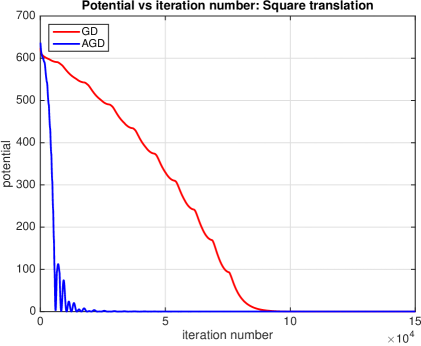
Figure 1: Convergence Comparison: Two binary images with squares in which the square is translated are registered. The value of the functional (to be minimized) versus the iteration number is shown for both gradient descent (GD) and accelerated gradient descent (AGD).

We now repeat the same experiment, but with different images to show that this behavior is not restricted to the particular choice of images, one a translation of the other. To this end, we choose the images again to be $50\times 50$. The first image has a square that is $17\times 17$ and the second image has a rectangle of size $20\times 14$ and is translated by $8$ pixels. We choose the regularity $\alpha=2$, since the regularity should be chosen smaller to account for the stretching and squeezing, resulting in a non-smooth flow field. A plot of results of this simulation is shown in Figure 2. Again accelerated gradient accelerates very quickly at the start, then oscillates and the oscillations die down and then it converges. This time the potential does not go to zero since the final flow is not a translation and thus the regularity term is non-zero. Gradient descent converges faster than the case of translation due to larger $\alpha$ and thus larger step size. However, it appears to be stuck in a higher energy configuration. In fact, gradient descent has not fully converged - gradient descent is slow in adapting to the scale changes and becomes extremely slow in stretching and squeezing in different directions. We verify that gradient descent has not fully converged by plotting just the first term of the potential, i.e., the reconstruction error, which is zero for accelerated gradient descent at convergence, indicating that the flow correctly reconstructs $I_{0}$ from $I_{1}$. On the other hand, gradient descent has an error of about $50$, indicating the flow does not fully warp $I_{1}$ to $I_{0}$, and therefore it not the correct flow. This does not appear to be a local minimum, just slow convergence.

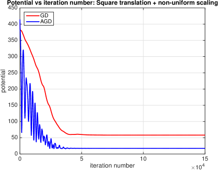
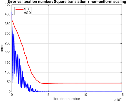
Figure 2: Convergence Comparison: Two images are registered, each are binary images. The first is a square and the second image is a translated and non-uniformly scaled version of the square in the first image. [Left]: The cost functional to be minimized versus the iteration number is shown for both gradient descent (GD) and accelerated gradient descent (AGD). AGD converges to a lower energy solution quicker. [Right]: Note that GD did not fully converge as the convergence is extremely slow in obtaining fine scale details of the non-uniform scaling. This is verified by plotting the image reconstruction error: $\|I_{1}\circ\phi-I_{0}\|$, which shows that AGD reconstructs $I_{0}$ with zero error.

We again repeat the same experiment, but with real images from a cardiac MRI sequence, in which the heart beats. The transformation relating the images is a general diffeomorphism that is not easily described as in the previous experiments. The images are of size $256\times 256$. We choose $\alpha=0.02$. A plot of the potential versus iteration number for both gradient descent (GD) and accelerated gradient descent (AGD) is shown in the left of Figure 3. The convergence is quicker for accelerated gradient descent. The right of Figure 3 shows the original images and the images warped under both the result from gradient descent and accelerated gradient descent, and that they both produce a similar correct warp, but accelerated gradient obtains the warp in much fewer iterations.

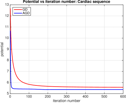
$I_{1}$	$I_{0}$
$I_{1}\circ\phi_{gd}$	$I_{1}\circ\phi_{agd}$

Figure 3: Convergence Comparison: Two MR cardiac images from a sequence are registered. The images are related through a general deformation. [Left]: A plot of the potential versus the iteration number in the minimization using gradient descent (GD) and accelerated gradient descent (AGD). AGD converges at a quicker rate. [Right]: The original images and the back-warped images using the recovered diffeomorphisms. Note that $I_{1}\circ\phi$ should appear close to $I_{0}$. Both methods seem to recover a similar transformation, but AGD recovers it faster.

IV-2 Convergence analysis versus parameter settings

We now analyze the convergence of accelerated gradient descent and gradient descent as a function of the regularity $\alpha$ and the image size. To this end, we first analyze an image pair of size $50\times 50$ in which one image has a square of size $16\times 16$ and the other image is the same square translated by $7$ pixels. We now vary $\alpha$ and analyze the convergence. In the left plot of Figure 4, we show the number of iterations until convergence versus the regularity $\alpha$. As $\alpha$ increases, the number of iterations for both gradient descent and accelerated gradient descent increase as expected since there is a inverse relationship between $\alpha$ and the step size. However, the number of iterations for accelerated gradient descent grows more slowly. In all cases, the algorithm is run until the flow field between successive iterations does not change according to a fixed tolerance. In all cases, the flow achieves the ground truth flow.

Next, we analyze the number of convergence iterations versus the image size. To this end, we again consider binary images with squares of size $16\times 16$ and translated by $7$ pixels. However, we vary the image size from $50\times 50$ to $200\times 200$. We fix $\alpha=8$. Now we show the number of iterations to convergence versus the image size. This is shown in the right plot of Figure 4. Gradient descent is impractically slow for all the sizes considered, and the number of iterations quickly increases with image size (it appears to be an exponential growth). Accelerated gradient descent, surprisingly, appears to have very little or no growth with respect to the image size. Of course one could use multi-scaling pyramid approaches to improve gradient descent, but as soon as one goes to finer scales, gradient descent is incredibly slow even when the images are related by small displacements. Simple acceleration makes standard gradient descent scalable with just a few extra local updates.

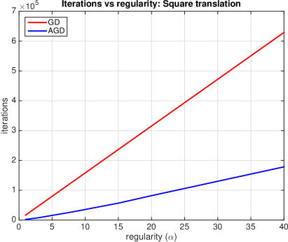
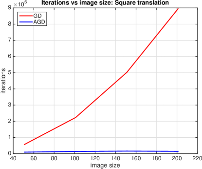
Figure 4: [Left]: Convergence Comparison as a Function of Regularity: Two binary images (a square and a translated square) are registered with varying amounts of regularization $\alpha$ for gradient descent (GD) and accelerated gradient descent (AGD). [Right]: Convergence Comparison as a Function of Image Size: We keep the squares in the images and $\alpha=3$ fixed, but we vary the size (height and width) of the image and compare GD with AGD. Very quickly, gradient descent becomes impractical due to extremely slow convergence.

IV-3 Analysis of Robustness to Noise

We now analyze the robustness of gradient descent and accelerated gradient descent to noise. We do this to simulate robustness to undesirable local minima. We choose to use salt and pepper noise to model possible clutter in the image. We consider images of size $50\times 50$. We fix $\alpha=1$ in all the simulations and vary the noise level; of course one could increase $\alpha$ to increase robustness to noise. However, we are interested in understanding the robustness to noise of the optimization algorithms themselves rather than changing the potential energy to better cope with noise. First, we consider a square of size $16\times 16$ in the first binary image and the same square translated by $4$ pixels in the second image. We plot the error in the flow (measured as the average endpoint error of the flow returned by the algorithm against ground truth flow) versus the noise level. The result is shown in the left plot of Figure 5. This shows that accelerated gradient descent degrades much slower than gradient descent. Figure 6 shows visual comparison of the final results where we show $I_{1}\circ\phi$ and compare it to $I_{0}$ for both accelerated gradient descent and gradient descent.

We repeat the same experiment to show that this trend is not just with this configuration of images. To this end, we experiment with $50\times 50$ images one with a square of size $15\times 15$ and a rectangle that is size $20\times 10$ and translated by $5$ pixels. We again fix the regularity to $\alpha=1$. The result of the experiment is plotted in the right of Figure 5. A similar trend of the previous experiment is observed: accelerated gradient descent degrades much less than gradient descent. Note we have measured accuracy as the average reconstruction error with the original (non-noisy) images. This is because the ground truth flow is not known. Figure 7 shows visual comparison of the final results.

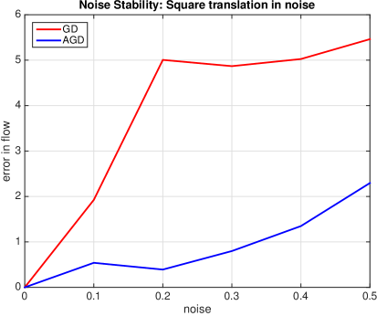
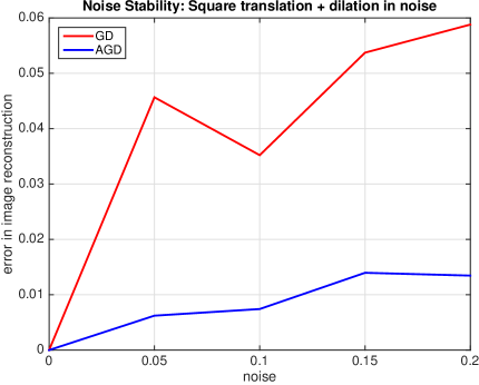
Figure 5: Analysis of Stability to Noise: We add salt and pepper noise with varying intensity to binary images and then register the images. We plot the error in the recovered flow of both gradient descent (GD) and accelerated gradient descent (AGD) versus the level of noise. The value of $\alpha$ is kept fixed. The error is measured by the average endpoint error of the flow. [Left]: The first image is formed from a square and the second image is the same square but translated. [Right]: The first image is a square and the second image is the non-uniformly scaled and translated square. The error is measured as the average image reconstruction error.

$\quad\quad\quad I_{1}\quad\quad$ $\quad\quad\quad I_{0}\quad$ $\quad\quad\quad I_{1}\circ\phi_{gd}$ $\quad\quad I_{1}\circ\phi_{agd}$	$\quad\quad\quad I_{1}\quad\quad$ $\quad\quad\quad I_{0}\quad$ $\quad\quad\quad I_{1}\circ\phi_{gd}$ $\quad\quad I_{1}\circ\phi_{agd}$
$\quad\sigma=0.0$	$\quad\sigma=0.1$
$\quad\sigma=0.2$	$\quad\sigma=0.3$
$\quad\sigma=0.4$	$\quad\sigma=0.5$

Figure 6: Visual Comparison on Square Translation in Noise Experiment. The above show the visual results of the noise robustness experiment. For each row group of images: the two original images, the warped image by gradient descent, and the warped image by accelerated gradient descent. The last two images should resemble the second if the registration is correct.

$\quad\quad\quad I_{1}\quad\quad$ $\quad\quad\quad I_{0}\quad$ $\quad\quad\quad I_{1}\circ\phi_{gd}$ $\quad\quad I_{1}\circ\phi_{agd}$	$\quad\quad\quad I_{1}\quad\quad$ $\quad\quad\quad I_{0}\quad$ $\quad\quad\quad I_{1}\circ\phi_{gd}$ $\quad\quad I_{1}\circ\phi_{agd}$
$\quad\sigma=0.00$	$\quad\sigma=0.05$
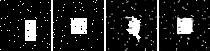
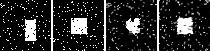
$\quad\sigma=0.10$	$\quad\sigma=0.15$
$\quad\sigma=0.20$

Figure 7: Visual Comparison on Square Non-Uniform Scaling and Translation in Noise Experiment. The above show the visual results of the noise robustness experiment. For each row group of images: the two original images, the warped image by gradient descent, and the warped image by accelerated gradient descent. The last two images should resemble the second if the registration is correct.

V Conclusion

We have generalized accelerated optimization, in particular Nesterov’s scheme, to infinite dimensional manifolds. This method is general and applies to optimizing any functional on an infinite dimensional manifold. We have demonstrated this for the class of diffeomorphisms motivated by variational optical flow problems in computer vision. The main objective of the paper was to introduce the formalism and derive the evolution equations that are PDEs. The evolution equations are natural extensions of mechanical principles from fluid mechanics, and in particular connect to optimal mass transport. They require additional evolution equations over gradient descent, i.e., a velocity evolution and a density evolution, but that does not significantly add to the cost of $L^{2}$ gradient descent per iteration since the updates are all local, i.e., computation of derivatives. Our numerical scheme to implement these equations used entropy conditions, which were employed to cope with shocks and fans of the underlying PDE. Our numerical scheme is not final and could be improved, and we plan to explore this in future work. Experiments on toy examples nevertheless demonstrated the advantages of speed and robustness to local minima over gradient descent, and illustrated the behavior of accelerated gradient descent. Just by simple acceleration, gradient descent, unusable in practice due to scalability with image size, became usable. One area that should be explored further is the choice of the time-explicit functions $a,b$ in the generalized Lagrangian. These were chosen to coincide with the choices to produce the continuum limit of Nesterov’s scheme finite dimensions, which are designed for the convex case to yield optimal convergence. Since the energies that we consider are non-convex, these may no longer be optimal. Of interest would be a design principle for choosing $a,b$ so as to obtain optimal convergence rates. A follow-up question would then be whether the discretization of the PDEs gives optimal rates in discrete-time. Another issue is that we assumed that the domain of the diffeomorphism was $\mathbb{R}^{n}$, but images are compact; we by-passed this complication by assuming periodic boundary conditions. Future work will look into proper treatment of the boundary.

-A Functional Gradients

Definition 1 (Functional Gradients).

Let $U:\mbox{Diff}(\mathbb{R}^{n})\to\mathbb{R}$. The gradient (or functional derivative) of $U$ with respect to $\phi\in\mbox{Diff}(\mathbb{R}^{n})$, denoted $\nabla U(\phi)$, is defined as the $\nabla U(\phi)\in T_{\phi}\mbox{Diff}(\mathbb{R}^{n})$ that satisfies

$$\delta U(\phi)\cdot v=\int_{\phi(\mathbb{R}^{n})}\nabla U(\phi)(x)\cdot v(x)\,\mathrm{d}x$$ (32)

for all $v\in T_{\phi}\mbox{Diff}(\mathbb{R}^{n})$. The left hand side is the directional derivative and is defined as

$$\delta U(\phi)\cdot v:=\left.\frac{\,\mathrm{d}{}}{\,\mathrm{d}{\varepsilon}}U(\phi+\varepsilon v)\right|_{\varepsilon=0}.$$ (33)

Note that $(\phi+\varepsilon v)(x)=\phi(x)+\varepsilon v(\phi(x))$ for $x\in\mathbb{R}^{n}$.

We now show the computation of the gradient for the illustrative potential (29) used in this paper. First, let us consider the data term $U_{1}(\phi)=\int_{\mathbb{R}^{n}}|I_{1}(\phi(x))-I_{0}(x)|^{2}\,\mathrm{d}x$ then

$$\delta U_{1}(\phi)\cdot\delta\phi=\int_{\mathbb{R}^{n}}2(I_{1}(\phi(x))-I_{0}(x))DI_{1}(\phi(x))\widehat{\delta\phi}(x)\,\mathrm{d}x=\int_{\phi(\mathbb{R}^{n})}2(I_{1}(x)-I_{0}(\psi(x)))DI_{1}(x)\delta\phi(x)\det{\nabla\psi(x)}\,\mathrm{d}x,$$

where $\widehat{\delta\phi}=\delta\phi\circ\phi$, $\psi=\phi^{-1}$ and we have performed a change of variables. Thus, $\nabla U_{1}=2\nabla I_{1}(I_{1}-I_{0}\circ\psi)\det{\nabla\psi}$. Now consider the regularity term $U_{2}(\phi)=\int_{\mathbb{R}^{n}}|\nabla(\phi(x)-x)|^{2}\,\mathrm{d}x$, then

$$\delta U(\phi)=2\int_{\mathbb{R}^{n}}\mbox{tr}\left({\nabla(\phi(x)-\mbox{id})^{T}\nabla\widehat{\delta\phi}(x)}\right)\,\mathrm{d}x=-\int_{\mathbb{R}^{n}}\Delta\phi(x)^{T}\delta\phi(x)\,\mathrm{d}x=\int_{\Omega}(\Delta\phi)(\psi(x))^{T}\delta\phi(x)\det{\nabla\psi(x)}\,\mathrm{d}x.$$

Note that in integration by parts, the boundary term vanishes since we assume that $\phi(x)=x$ as $|x|\to\infty$. Thus, $\nabla U_{2}=(\Delta\phi)\circ\psi\det{\nabla\psi}$.

-B Stationary Conditions

Lemma 1 (Stationary Condition for the Mapping).

The stationary condition of the action (11) for the mapping is

$$\partial_{t}\lambda+\mbox{div}\left({v\lambda^{T}}\right)^{T}=(\nabla\psi)^{-1}\nabla U(\phi).$$ (34)

Proof.

We compute the variation of $A$ (defined in (11)) with respect to the mapping $\phi$. The only terms in the action that depend on the mapping are $U$ and the Lagrange multiplier term associated with the mapping. Taking the variation w.r.t the potenial term gives

$$-\int\int_{\phi(\mathbb{R}^{n})}\nabla U(\phi)\cdot\delta\phi\,\mathrm{d}x\,\mathrm{d}t.$$

Now the variation with respect to the Lagrange multiplier term:

$$\int\int_{\phi(\mathbb{R}^{n})}\lambda^{T}[\partial_{t}\widehat{\delta\psi}+D(\widehat{\delta\psi})v]\,\mathrm{d}x\,\mathrm{d}t=-\int\int_{\phi(\mathbb{R}^{n})}[\partial_{t}\lambda^{T}+\mbox{div}\left({v\lambda^{T}}\right)]\widehat{\delta\psi}\,\mathrm{d}x\,\mathrm{d}t,$$

where we have integrated by parts, the $\mbox{div}\left({\cdot}\right)$ of a matrix means the divergence of each of the columns, resulting in a row vector, and $\widehat{\delta\psi}=\delta\psi\circ\psi$. Note that we can take the variation of $\psi(\phi(x))=x$ to obtain

$$\widehat{\delta\psi}\circ\phi(x)+[D\psi(\phi(x))]\widehat{\delta\phi}(x)=0,$$

or

$$\widehat{\delta\psi}(y)=-[D\psi(y)]\delta\phi(y).$$

Therefore,

$$\delta A\cdot\delta\phi=\int\int_{\phi(\mathbb{R}^{n})}\left\{(\nabla\psi)\left[\partial_{t}\lambda+\mbox{div}\left({v\lambda^{T}}\right)^{T}\right]-\nabla U(\phi)\right\}\cdot\delta\phi\,\mathrm{d}x\,\mathrm{d}t.$$ (35)

∎

Lemma 2 (Stationary Condition for the Velocity).

The stationary condition of the action (11) arising from the velocity is

$$\rho v+(\nabla\psi)\lambda-\rho\nabla\mu=0.$$ (36)

Proof.

We compute the variation w.r.t the kinetic energy:

$$\delta T\cdot\delta v=\int_{\phi(\mathbb{R}^{n})}\rho v\cdot\delta v\,\mathrm{d}x.$$

The variation of the Lagrange multiplier terms is

$$\int\int_{\phi(\mathbb{R}^{n})}\lambda^{T}(D\psi)\delta v-\rho\nabla\mu\cdot\delta v\,\mathrm{d}x\,\mathrm{d}t=\int\int_{\phi(\mathbb{R}^{n})}[(\nabla\psi)\lambda-\rho\nabla\mu]\cdot\delta v\,\mathrm{d}x\,\mathrm{d}t.$$

Therefore,

$$\delta A\cdot\delta v=\int\int_{\phi(\mathbb{R}^{n})}[\rho v+(\nabla\psi)\lambda-\rho\nabla\mu]\cdot\delta v\,\mathrm{d}x\,\mathrm{d}t.$$ (37)

∎

Lemma 3 (Stationary Condition for the Density).

The stationary condition of the action (11) arising from the velocity is

$$\partial_{t}\mu+(D\mu)v=\frac{1}{2}|v|^{2}.$$ (38)

Proof.

Note that the terms that contain the density in (11) are the kinetic energy and the Lagrange multiplier corresponding to the density. We see that

$$\delta A\cdot\delta\rho=\int\int_{\phi(\mathbb{R}^{n})}\frac{1}{2}|v|^{2}\delta\rho-(\partial_{t}\mu+\nabla\mu\cdot v)\delta\rho\,\mathrm{d}x\,\mathrm{d}t,$$ (39)

which yields the lemma. ∎

-C Velocity Evolution

Lemma 4.

Given that $(\nabla\psi)\lambda=w$, we have that

$$\partial_{t}\lambda+(D\lambda)v+\lambda\mbox{div}\left({v}\right)=(\nabla\psi)^{-1}[\partial_{t}w+(Dw)v+(\nabla v)w+w\mbox{div}\left({v}\right)]$$ (40)

Proof.

Define the Hessian as follows:

$$[D^{2}\psi]_{ijk}=\partial_{x_{i}x_{j}}^{2}\psi^{k},\quad[D^{2}\psi(a,b)]_{k}=\sum_{ij}\partial_{x_{i}x_{j}}^{2}\psi^{k}a_{i}b_{j}.$$

We compute

$$\{D[(\nabla\psi)\lambda]\}_{ij}=\partial_{x_{j}}[(\nabla\psi)\lambda]_{i}=\partial_{x_{j}}\sum_{l}\partial_{x_{i}}\psi^{l}\lambda_{l}=\sum_{l}(\partial^{2}_{x_{j}x_{i}}\psi^{l}\lambda_{l})+\partial_{x_{i}}\psi^{l}\partial_{x_{j}}\lambda_{l}.$$

Therefore,

$$D[(\nabla\psi)\lambda]=D^{2}\psi(\cdot,\cdot)\cdot\lambda+(\nabla\psi)(D\lambda)$$

Since $D[(\nabla\psi)\lambda]=Dw$ then solving for $D\lambda$ gives

$$D\lambda=(\nabla\psi)^{-1}[Dw-D^{2}\psi(\cdot,\cdot)\cdot\lambda],$$

so

$$(D\lambda)v=(\nabla\psi)^{-1}[(Dw)v-D^{2}\psi(\cdot,v)\cdot\lambda].$$ (41)

Now differentiating $(\nabla\psi)\lambda=w$ w.r.t $t$, we have

$$(\nabla\partial_{t}\psi)\lambda+(\nabla\psi)\partial_{t}\lambda=\partial_{t}w,\quad\mbox{or}\quad\partial_{t}\lambda=(\nabla\psi)^{-1}[\partial_{t}w-(\nabla\partial_{t}\psi)\lambda]$$

Note that $\partial_{t}\psi=-(D\psi)v$ so

$$\partial_{t}\lambda=(\nabla\psi)^{-1}\left\{\partial_{t}w+\nabla[(D\psi)v]\lambda\right\}.$$ (42)

Now computing $\nabla[(D\psi)v]$ yields

$$\{\nabla[(D\psi)v)]\}_{lk}=\partial_{x_{l}}\sum_{i}\partial_{x_{i}}\psi^{k}v^{i}=\sum_{i}\partial_{x_{l}}\partial_{x_{i}}\psi^{k}v^{i}+\partial_{x_{i}}\psi^{k}\partial_{x_{l}}v^{i}.$$

Then multiplying the above matrix by $\lambda$ gives

$$\{\nabla[(D\psi)v)]\lambda\}_{l}=\sum_{ik}\partial_{x_{l}}\partial_{x_{i}}\psi^{k}v^{i}\lambda^{k}+\partial_{x_{i}}\psi^{k}\partial_{x_{l}}v^{i}\lambda^{k},$$

which in matrix form is

$$\nabla[(D\psi)v)]\lambda=D^{2}\psi(\cdot,v)\cdot\lambda+(\nabla v)(\nabla\psi)\lambda=D^{2}\psi(\cdot,v)\cdot\lambda+(\nabla v)w$$

Therefore, (42) becomes

$$\partial_{t}\lambda=(\nabla\psi)^{-1}[\partial_{t}w+D^{2}\psi(\cdot,v)\cdot\lambda+(\nabla v)w].$$

Combining the previous with (41) and noting that $\lambda\mbox{div}\left({v}\right)=(\nabla\psi)^{-1}w\mbox{div}\left({v}\right)$ yields

$$\partial_{t}\lambda+(D\lambda)v+\lambda\mbox{div}\left({v}\right)=(\nabla\psi)^{-1}[\partial_{t}w+(Dw)v+(\nabla v)w+w\mbox{div}\left({v}\right)].$$

∎

Lemma 5.

If $w=\rho(\nabla\mu-v)$, then

$$\partial_{t}w+(Dw)v+(\nabla v)w+w\mbox{div}\left({v}\right)=-\rho[\partial_{t}v+(Dv)v].$$ (43)

Proof.

Differentiating $w=\rho(\nabla\mu-v)$, we have

$$\partial_{t}w =(\partial_{t}\rho)(\nabla\mu-v)+\rho(\nabla\partial_{t}\mu-\partial_{t}v)$$

$$Dw =(\nabla\mu-v)(D\rho)+\rho[D(\nabla\mu)-Dv].$$

Therefore,

$$\partial_{t}w+(Dw)v+(\nabla v)w+w\mbox{div}\left({v}\right) =(\nabla\mu-v)(\partial_{t}\rho+\nabla\rho\cdot v)+\rho[\nabla\partial_{t}\mu-\partial_{t}v+D(\nabla\mu)v-(Dv)v]$$

$$+\rho(\nabla v)(\nabla\mu-v)+\rho(\nabla\mu-v)\mbox{div}\left({v}\right)$$

$$=(\nabla\mu-v)(\partial_{t}\rho+\nabla\rho\cdot v+\rho\mbox{div}\left({v}\right))$$

$$+\rho[\nabla\partial_{t}\mu-\partial_{t}v+D(\nabla\mu)v-(Dv)v+(\nabla v)(\nabla\mu-v)].$$

Note that $\partial_{t}\rho+\nabla\rho\cdot v+\rho\mbox{div}\left({v}\right)=\partial_{t}\rho+\mbox{div}\left({\rho v}\right)=0$, due to the continuity equation. Therefore,

$$\partial_{t}w+(Dw)v+(\nabla v)w+w\mbox{div}\left({v}\right) =\rho[-\partial_{t}v-(Dv)v-(\nabla v)v+\nabla\partial_{t}\mu+D(\nabla\mu)v+(\nabla v)(\nabla\mu)]$$

$$=\rho\left\{-\partial_{t}v-(Dv)v-(\nabla v)v+\nabla[\partial_{t}\mu+(D\mu)v]\right\}.$$

By the stationary condition for the density, $\partial_{t}\mu+(D\mu)v=1/2|v|^{2}$, so $\nabla[\partial_{t}\mu+(D\mu)v]=(\nabla v)v$, which gives the lemma. ∎

Theorem .1 (Velocity Evolution).

The evolution equation for the velocity arising from the stationarity of the action integral is

$$\rho[\partial_{t}v+(Dv)v]=-\nabla U(\phi).$$ (44)

Proof.

This is a combination of Lemmas 1, 4, and 5. ∎

-D Stationary Conditions for the Dissipative Case

Theorem .2 (Stationary Conditions for the Path of Least Action: Dissipative Case).

The stationary conditions of the path for the action

$$A =\int\left[aT(v)-bU(\phi)\right]\,\mathrm{d}t+\int\int_{\mathbb{R}^{n}}\lambda^{T}[\partial_{t}\psi_{t}+(D\psi)v]\,\mathrm{d}x\,\mathrm{d}t-\int\int_{\mathbb{R}^{n}}\left[\partial_{t}\mu+\nabla\mu\cdot v\right]\rho\,\mathrm{d}x\,\mathrm{d}t,$$ (45)

are

$$\partial_{t}\lambda+(D\lambda)v+\lambda\mbox{div}\left({v}\right) =b(\nabla\psi)^{-1}\nabla U(\phi)$$ (46)

$$a\rho v+(\nabla\psi)\lambda-\rho\nabla\mu =0$$ (47)

$$\partial_{t}\mu+\nabla\mu\cdot v =\frac{1}{2}a|v|^{2}.$$ (48)

Proof.

Note that

$$\nabla[bU](\phi) =b\nabla U(\phi)$$

$$\delta[aT]\cdot\delta\rho =\int_{\phi(\mathbb{R}^{n})}\frac{1}{2}a|v|^{2}\delta\rho\,\mathrm{d}x$$

$$\delta[aT]\cdot\delta v =\int_{\phi(\mathbb{R}^{n})}a\rho v\cdot\delta v\,\mathrm{d}x.$$

Therefore, using (35) and replacing $\nabla U(\phi)$ with $b\nabla U(\phi)$, we have

$$\delta A\cdot\delta\phi=\int\int_{\phi(\mathbb{R}^{n})}\left\{(\nabla\psi)\left[\partial_{t}\lambda+\mbox{div}\left({v\lambda^{T}}\right)^{T}\right]-b\nabla U(\phi)\right\}\cdot\delta\phi\,\mathrm{d}x\,\mathrm{d}t,$$

which yields the stationary condition on the mapping. Also, updating (37) yields

$$\delta A\cdot\delta v=\int\int_{\phi(\mathbb{R}^{n})}[a\rho v+(\nabla\psi)\lambda-\rho\nabla\mu]\cdot\delta v\,\mathrm{d}x\,\mathrm{d}t,$$

which yields the stationary condition for the velocity. Finally, updating (39) yields

$$\delta A\cdot\delta\rho=\int\int_{\phi(\mathbb{R}^{n})}\frac{1}{2}a|v|^{2}\delta\rho-(\partial_{t}\mu+\nabla\mu\cdot v)\delta\rho\,\mathrm{d}x\,\mathrm{d}t,$$

and that yields the last stationary condition. ∎

Theorem .3 (Evolution Equations for the Path of Least Action: Dissipative Case).

The evolution equations for the stationary conditions of the action in (45) is

$$\rho[\partial_{t}(av)+a(Dv)v]=-b\nabla U(\phi).$$ (49)

Proof.

Let $w=\rho(\nabla\mu-av)$ then

$$\partial_{t}w =(\partial_{t}\rho)(\nabla\mu-av)+\rho(\nabla\partial_{t}\mu-\partial_{t}(av))$$

$$Dw =(\nabla\mu-av)(D\rho)+\rho[D(\nabla\mu)-aDv].$$

Then

$$\partial_{t}w+(Dw)v+(\nabla v)w+w\mbox{div}\left({v}\right) =g(\nabla\mu-av)(\partial_{t}\rho+\nabla\rho\cdot v)+\rho[\nabla\partial_{t}\mu-\partial_{t}(av)+D(\nabla\mu)v-a(Dv)v]$$

$$+\rho(\nabla v)(\nabla\mu-av)+\rho(\nabla\mu-av)\mbox{div}\left({v}\right)$$

$$=(\nabla\mu-av)(\partial_{t}\rho+\nabla\rho\cdot v+\rho\mbox{div}\left({v}\right))$$

$$+\rho[\nabla\partial_{t}\mu-\partial_{t}(av)+D(\nabla\mu)v-a(Dv)v+(\nabla v)(\nabla\mu-av)]$$

$$=\rho\left\{-\partial_{t}(av)-a(Dv)v-a(\nabla v)v+\nabla[\partial_{t}\mu+(D\mu)v]\right\}$$

$$=\rho\left\{-\partial_{t}(av)-a(Dv)v\right\}.$$

By Lemma 4 and the previous expression, we have our result. ∎

-E Discretization

We present the discretization of the velocity PDE (26) first. In one dimension, the terms involving $v$ are Burger’s equation, which is known to produce shocks. We thus use an entropy scheme. Writing the PDE component-wise, we get

$$\partial_{t}v_{1} =-\frac{1}{2}\partial_{x_{1}}(v_{1})^{2}-v_{2}\partial_{x_{2}}v_{1}-\frac{3}{t}v_{1}-\frac{1}{\rho}(\nabla U)_{1}$$ (50)

$$\partial_{t}v_{2} =-\frac{1}{2}\partial_{x_{2}}(v_{2})^{2}-v_{1}\partial_{x_{1}}v_{1}-\frac{3}{t}v_{2}-\frac{1}{\rho}(\nabla U)_{2},$$ (51)

where the subscript indicates the component of the vector. We use forward Euler for the time derivative, and for the first term on the right hand side, we use an entropy scheme for Burger’s equation which results in the following discretization:

$$\partial_{x_{1}}(v_{1})^{2}(x)\approx\max\{v_{1}(x),0\}^{2}-\min\{v_{1}(x),0\}^{2}+\min\{v_{1}(x_{1}+\Delta x,x_{2}),0\}^{2}-\max\{v_{1}(x_{1}+\Delta x,x_{2}),0\}^{2},$$

where $\Delta x$ is the spatial sampling size, and the $\partial_{x_{2}}(v_{2})^{2}$ follows similarly. For the second term on the right hand side of (50), we follow the discretization of a transport equation using an up-winding scheme, which yields the following discretization:

$$v_{2}(x)\partial_{x_{2}}v_{1}(x)\approx v_{2}(x)\cdot\begin{cases}v_{1}(x_{1},x_{2})-v_{1}(x_{1},x_{2}-\Delta x)&v_{2}(x)>0\\ v_{1}(x_{1},x_{2}+\Delta x)-v_{1}(x_{1},x_{2})&v_{2}(x)<0\end{cases}.$$

With regards to the gradient of potential, if we use the potential (29), then all the derivatives are discretized using central differences, as the key term is a diffusion. The step size $\Delta t/\Delta x<1/\max_{x}\{|v(x)|,|Dv(x)|\}$.

The backward map $\psi$ evolves according to a transport PDE (9), and thus an up-winding scheme similar to the transport term in the velocity term is used. For the discretization of the continuity equation, we use a staggered grid (so that the values of $v$ are defined in between grid points and $\rho$ is defined at the grid points). The discretization is just the sum of the fluxes coming into the point:

$$-\mbox{div}\left({\rho(x)v(x)}\right)\approx\sum_{i=1}^{2}\left[-v_{i}(x)\begin{cases}\rho(x)&v_{i}(x)>0\\ \rho(x+\Delta x_{i})&v_{i}(x)<0\end{cases}+v_{i}(x-\Delta x_{i})\begin{cases}\rho(x-\Delta x_{i})&v_{1}(x-\Delta x_{i})>0\\ \rho(x)&v_{1}(x-\Delta x_{i})<0\end{cases}\right],$$

where $\Delta x_{i}$ denotes the vector of the spatial increment $\Delta x$ in the $i^{\text{th}}$ coordinate direction, $v_{1}(x)$ denotes the velocity defined at the midpoint between $(x_{1},x_{2})$ and $(x_{1}+\Delta x,x_{2})$, and $v_{2}(x)$ denotes the velocity defined at the midpoint between $(x_{1},x_{2})$ and $(x_{1},x_{2}+\Delta x)$. The term $\partial_{t}\rho(x)$ is discretized with forward Euler. This scheme is guaranteed to preserve mass.

References

- [1] A. Wibisono, A. C. Wilson, and M. I. Jordan, “A variational perspective on accelerated methods in optimization,” Proceedings of the National Academy of Sciences, vol. 113, no. 47, pp. E7351–E7358, 2016.
- [2] S. Bubeck, Y. T. Lee, and M. Singh, “A geometric alternative to nesterov’s accelerated gradient descent,” CoRR, vol. abs/1506.08187, 2015.
- [3] N. Flammarion and F. Bach, “From averaging to acceleration, there is only a step-size,” in Proceedings of Machine Learning Research, vol. 40, 2015, pp. 658–695.
- [4] S. Ghadimi and G. Lan, “Accelerated gradient methods for nonconvex nonlinear and stochastic programming,” Math. Program., vol. 156, no. 1-2, pp. 59–99, 2016.
- [5] C. Hu, W. Pan, and J. T. Kwok, “Accelerated gradient methods for stochastic optimization and online learning,” in Advances in Neural Information Processing Systems 22, Y. Bengio, D. Schuurmans, J. D. Lafferty, C. K. I. Williams, and A. Culotta, Eds. Curran Associates, Inc., 2009, pp. 781–789.
- [6] S. Ji and J. Ye, “An accelerated gradient method for trace norm minimization,” in Proceedings of the 26th Annual International Conference on Machine Learning, ser. ICML ’09, 2009, pp. 457–464.
- [7] V. Jojic, S. Gould, and D. Koller, “Accelerated dual decomposition for map inference,” in Proceedings of the 27th International Conference on International Conference on Machine Learning, ser. ICML’10, 2010, pp. 503–510.
- [8] W. Krichene, A. Bayen, and P. L. Bartlett, “Accelerated mirror descent in continuous and discrete time,” in Advances in Neural Information Processing Systems 28, C. Cortes, N. D. Lawrence, D. D. Lee, M. Sugiyama, and R. Garnett, Eds. Curran Associates, Inc., 2015, pp. 2845–2853.
- [9] H. Li and Z. Lin, “Accelerated proximal gradient methods for nonconvex programming,” in Advances in Neural Information Processing Systems 28, C. Cortes, N. D. Lawrence, D. D. Lee, M. Sugiyama, and R. Garnett, Eds. Curran Associates, Inc., 2015, pp. 379–387.
- [10] Y. Nesterov, “Smooth minimization of non-smooth functions,” Math. Program., vol. 103, no. 1, pp. 127–152, 2005.
- [11] ——, “Accelerating the cubic regularization of newton’s method on convex problems,” Math. Program., vol. 112, no. 1, pp. 159–181, 2008.
- [12] ——, “A method of solving a convex programming problem with convergence rate o (1/k2),” in Soviet Mathematics Doklady, vol. 27, 1983, pp. 372–376.
- [13] H. Zhang, S. J. Reddi, and S. Sra, “Riemannian svrg: fast stochastic optimization on riemannian manifolds,” in Advances in Neural Information Processing Systems, 2016, pp. 4592–4600.
- [14] Y. Liu, F. Shang, J. Cheng, H. Cheng, and L. Jiao, “Accelerated first-order methods for geodesically convex optimization on riemannian manifolds,” in Advances in Neural Information Processing Systems, 2017, pp. 4875–4884.
- [15] R. Hosseini and S. Sra, “An alternative to em for gaussian mixture models: Batch and stochastic riemannian optimization,” arXiv preprint arXiv:1706.03267, 2017.
- [16] V. I. Arnol’d, Mathematical methods of classical mechanics. Springer Science & Business Media, 2013, vol. 60.
- [17] J. E. Marsden and T. S. Ratiu, Introduction to mechanics and symmetry: a basic exposition of classical mechanical systems. Springer Science & Business Media, 2013, vol. 17.
- [18] A. J. Yezzi and G. Sundaramoorthi, “Accelerated optimization in the PDE framework: Formulations for the active contour case,” CoRR, vol. abs/1711.09867, 2017. [Online]. Available: http://arxiv.org/abs/1711.09867
- [19] J. A. Sethian, Level set methods and fast marching methods: evolving interfaces in computational geometry, fluid mechanics, computer vision, and materials science. Cambridge university press, 1999, vol. 3.
- [20] G. Sundaramoorthi, A. Yezzi, and A. Mennucci, “Sobolev active contours,” in Variational, Geometric and Level Set Methods in Computer Vision, ser. Lecture Notes in Computer Science. Springer, 2005, pp. 109–120.
- [21] M. F. Beg, M. I. Miller, A. Trouvé, and L. Younes, “Computing large deformation metric mappings via geodesic flows of diffeomorphisms,” International journal of computer vision, vol. 61, no. 2, pp. 139–157, 2005.
- [22] G. Charpiat, R. Keriven, J.-P. Pons, and O. Faugeras, “Designing spatially coherent minimizing flows for variational problems based on active contours,” in Computer Vision, 2005. ICCV 2005. Tenth IEEE International Conference on, vol. 2. IEEE, 2005, pp. 1403–1408.
- [23] G. Sundaramoorthi, A. Yezzi, and A. C. Mennucci, “Sobolev active contours,” International Journal of Computer Vision, vol. 73, no. 3, pp. 345–366, 2007.
- [24] G. Charpiat, P. Maurel, J.-P. Pons, R. Keriven, and O. Faugeras, “Generalized gradients: Priors on minimization flows,” International journal of computer vision, vol. 73, no. 3, pp. 325–344, 2007.
- [25] G. Sundaramoorthi, A. Yezzi, and A. Mennucci, “Coarse-to-fine segmentation and tracking using sobolev active contours,” IEEE Transactions on Pattern Analysis and Machine Intelligence, vol. 30, no. 5, pp. 851–864, 2008.
- [26] G. Sundaramoorthi, A. Yezzi, A. C. Mennucci, and G. Sapiro, “New possibilities with sobolev active contours,” International journal of computer vision, vol. 84, no. 2, pp. 113–129, 2009.
- [27] A. Mennucci, A. Yezzi, and G. Sundaramoorthi, “Sobolev–type metrics in the space of curves,” Interfaces and Free Boundaries, no. 10, pp. 423–445, 2008.
- [28] G. Sundaramoorthi, A. Mennucci, S. Soatto, and A. Yezzi, “A new geometric metric in the space of curves, and applications to tracking deforming objects by prediction and filtering,” SIAM Journal on Imaging Sciences, vol. 4, no. 1, pp. 109–145, 2011.
- [29] Y. Yang and G. Sundaramoorthi, “Shape tracking with occlusions via coarse-to-fine region-based sobolev descent,” IEEE transactions on pattern analysis and machine intelligence, vol. 37, no. 5, pp. 1053–1066, 2015.
- [30] E. Klassen, A. Srivastava, M. Mio, and S. H. Joshi, “Analysis of planar shapes using geodesic paths on shape spaces,” IEEE transactions on pattern analysis and machine intelligence, vol. 26, no. 3, pp. 372–383, 2004.
- [31] P. W. Michor, D. Mumford, J. Shah, and L. Younes, “A metric on shape space with explicit geodesics,” arXiv preprint arXiv:0706.4299, 2007.
- [32] M. Micheli, P. W. Michor, and D. Mumford, “Sobolev metrics on diffeomorphism groups and the derived geometry of spaces of submanifolds,” Izvestiya: Mathematics, vol. 77, no. 3, p. 541, 2013.
- [33] M. Bauer, M. Bruveris, and P. W. Michor, “Overview of the geometries of shape spaces and diffeomorphism groups,” Journal of Mathematical Imaging and Vision, vol. 50, no. 1-2, pp. 60–97, 2014.
- [34] C. Villani, Topics in optimal transportation. American Mathematical Soc., 2003, no. 58.
- [35] W. Gangbo and R. J. McCann, “The geometry of optimal transportation,” Acta Mathematica, vol. 177, no. 2, pp. 113–161, 1996.
- [36] S. Angenent, S. Haker, and A. Tannenbaum, “Minimizing flows for the monge–kantorovich problem,” SIAM journal on mathematical analysis, vol. 35, no. 1, pp. 61–97, 2003.
- [37] J.-D. Benamou and Y. Brenier, “A computational fluid mechanics solution to the monge-kantorovich mass transfer problem,” Numerische Mathematik, vol. 84, no. 3, pp. 375–393, 2000.
- [38] M. I. Miller, A. Trouvé, and L. Younes, “Geodesic shooting for computational anatomy,” Journal of mathematical imaging and vision, vol. 24, no. 2, pp. 209–228, 2006.
- [39] B. K. Horn and B. G. Schunck, “Determining optical flow,” Artificial intelligence, vol. 17, no. 1-3, pp. 185–203, 1981.
- [40] M. J. Black and P. Anandan, “The robust estimation of multiple motions: Parametric and piecewise-smooth flow fields,” Computer vision and image understanding, vol. 63, no. 1, pp. 75–104, 1996.
- [41] T. Brox, A. Bruhn, N. Papenberg, and J. Weickert, “High accuracy optical flow estimation based on a theory for warping,” in European conference on computer vision. Springer, 2004, pp. 25–36.
- [42] A. Wedel, T. Pock, C. Zach, H. Bischof, and D. Cremers, “An improved algorithm for tv-l 1 optical flow,” in Statistical and geometrical approaches to visual motion analysis. Springer, 2009, pp. 23–45.
- [43] D. Sun, S. Roth, and M. J. Black, “Secrets of optical flow estimation and their principles,” in Computer Vision and Pattern Recognition (CVPR), 2010 IEEE Conference on. IEEE, 2010, pp. 2432–2439.
- [44] Y. Yang and G. Sundaramoorthi, “Modeling self-occlusions in dynamic shape and appearance tracking,” in Computer Vision (ICCV), 2013 IEEE International Conference on. IEEE, 2013, pp. 201–208.
- [45] Y. Yang, G. Sundaramoorthi, and S. Soatto, “Self-occlusions and disocclusions in causal video object segmentation,” in Proceedings of the IEEE International Conference on Computer Vision, 2015, pp. 4408–4416.
- [46] M. P. Do Carmo, Riemannian geometry. Birkhauser, 1992.
- [47] Y. Nesterov, Introductory Lectures on Convex Optimization: A Basic Course, 1st ed. Springer Publishing Company, Incorporated, 2014.
- [48] ——, “Gradient methods for minimizing composite functions,” Math. Program., vol. 140, no. 1, pp. 125–161, 2013.
- [49] Y. Nesterov and B. T. Polyak, “Cubic regularization of newton method and its global performance,” Math. Program., vol. 108, no. 1, pp. 177–205, 2006.
- [50] W. Su, S. Boyd, and E. Candès, “A differential equation for modeling nesterov’s accelerated gradient method: Theory and insights,” in Advances in Neural Information Processing Systems, 2014, pp. 2510–2518.
- [51] D. G. Ebin and J. Marsden, “Groups of diffeomorphisms and the motion of an incompressible fluid,” Annals of Mathematics, pp. 102–163, 1970.
- [52] M. G. Crandall and P.-L. Lions, “Viscosity solutions of hamilton-jacobi equations,” Transactions of the American Mathematical Society, vol. 277, no. 1, pp. 1–42, 1983.
- [53] E. Rouy and A. Tourin, “A viscosity solutions approach to shape-from-shading,” SIAM Journal on Numerical Analysis, vol. 29, no. 3, pp. 867–884, 1992.