Phase transition, scaling of moments, and order-parameter distributions in Brownian particles and branching processes with finite-size effects

Abstract

We revisit the problem of Brownian diffusion with drift in order to study finite-size effects in the geometric Galton-Watson branching process. This is possible because of an exact mapping between one-dimensional random walks and geometric branching processes, known as the Harris walk. In this way, first-passage times of Brownian particles are equivalent to sizes of trees in the branching process (up to a factor of proportionality). Brownian particles that reach a distant boundary correspond to percolating trees, and those that do not correspond to non-percolating trees. In fact, both systems display a second-order phase transition between “insulating” and “conducting” phases, controlled by the drift velocity in the Brownian system. In the limit of large system size, we obtain exact expressions for the Laplace transforms of the probability distributions and their first and second moments. These quantities are also shown to obey finite-size scaling laws.

I Introduction

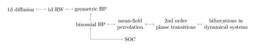
Figure 1: Relations between different physical processes and models, with abbreviations RW (random walk), BP (Galton-Watson branching process), SOC (self-organized critical phenomena) Jensen ; Christensen_Moloney ; Watkins_25years . BP with geometric and binomial offspring distribution share the same critical properties due to universality.

Random walks and rooted trees are important models in probability theory and statistical physics Harris52 . Random walks Weiss_Rubin ; Weiss_RW ; Klafter_Sokolov provide a microscopic model for diffusion processes Crank_diffusion , and rooted trees are the geometric representation of branching processes Harris_original ; branching_biology . The Galton-Watson process, which is the simplest branching process and is at the heart of self-organized-critical behavior Zapperi_branching ; Corral_FontClos , is essentially the same as mean-field percolation Aharony ; Christensen_Moloney when the offspring distribution of the former is binomial. Percolation, meanwhile, is one of the simplest examples of a second-order phase transition Stanley ; Yeomans1992 ; munoz_colloquium . Moreover, important characteristics of phase transitions also show up in bifurcations in low-dimensional dynamical systems Corral_Alseda_Sardanyes . An exact, purely geometric mapping between walks and rooted trees was presented in Ref. Harris52 , thereby connecting results from random walks to branching processes and beyond Font_clos_molon . Figure 1 offers a scheme for these relations.

This mapping, known as the Harris walk, implies that a realization of a finite-size geometric Galton-Watson branching process with no more than $L$ generations corresponds (exactly) to a random walker confined between absorbing and reflecting boundaries (at $X=0$ and $X=L$, respectively). Recently, Font-Clos and Moloney Font_clos_molon applied this mapping to derive the distribution of the size of the percolating clusters in a finite Bethe lattice, by using the first-passage time to the origin of a Brownian particle conditioned to first reach $L$. In the critical case (unbiased diffusion), a Kolmogorov-Smirnov distribution is obtained (as in Ref. Botet ). In the subcritical case (diffusion with negative drift) these authors find that the size of the percolating cluster follows Gaussian statistics, whereas in the supercritical case (diffusion with positive drift), an exponential-like distribution is reported.

In this work we follow the approach of Ref. Font_clos_molon and use the first passage-time in a diffusion process to calculate the size distribution of both percolating and non-percolating clusters in a geometric Galton-Watson process with a finite number of generations. First, we solve the corresponding diffusion problem and derive analytical expressions and scaling laws (Sec. 2); then we translate the results to the random-walk picture (Sec. 3); and finally, by means of the mapping from trees to walks Harris52 , we obtain the properties of the associated branching process. A discussion about the most appropriate definition of an order parameter in these systems is also provided. Our main focus is the size distribution of all clusters (whether they percolate or not). Given that the percolating case was thoroughly studied in Font_clos_molon , we will only provide details for the non-percolating case.

II First-passage times via the diffusion equation

Consider the one-dimensional diffusion equation with drift,

$$\frac{\partial c}{\partial t}+v\frac{\partial c}{\partial x}=D\frac{\partial^{2}c}{\partial x^{2}}$$ (1)

which describes the evolution of the concentration $c(x,t)$ of particles at position $x$ and time $t$, with drift velocity $v$ and diffusion constant $D$. Both position and time are continuous. We will work in a finite interval, $0\leq x\leq\ell$, with $\ell$ playing the role of system size ($X$ and $L$ mentioned in the introduction are dimensionless versions of $x$ and $\ell$). Following Redner Redner , first-passage times are most readily obtained by applying the Laplace transform $c(x,s)=\int_{0}^{\infty}e^{-st}c(x,t)dt$ to the diffusion equation, yielding

$$sc(x,s)-c(x,t=0)+vc^{\prime}(x,s)=Dc^{\prime\prime}(x,s),$$ (2)

where the prime denotes a derivative with respect to $x$.

II.1 Absorbing boundaries

First-passage time probability densities $f(t)$ are obtained from spatial concentration gradients at absorbing boundaries Redner . To see this, we track the rate of particle loss from the interval $0\leq x\leq\ell$:

$$f(t)=-\frac{d}{dt}\int_{0}^{\ell}c(x,t)dx =-\int_{0}^{\ell}D\frac{\partial^{2}c}{\partial x^{2}}\,dx+\int_{0}^{\ell}v\frac{\partial c}{\partial x}\,dx$$ (3)

$$=\left.-D\frac{\partial c}{\partial x}\right|_{x=\ell}+\left.D\frac{\partial c}{\partial x}\right|_{x=0},$$ (4)

where we have made use of the normalization of $c(x,t)$ for $t=0$ and of the absorbing boundary conditions at $x=0$ and $x=\ell$:

$$c(x=0,t)=c(x=\ell,t)=0.$$ (5)

Note that the terms in the above sum above are not probability densities themselves (because they are not normalized). Rather, they are the net outflux of particles at each boundary, so that $f(t)=j_{\ell}(t)+j_{0}(t)$. The Laplace transform of the probability density can therefore be written as

$$f(s)=j_{\ell}(s)+j_{0}(s)=-Dc^{\prime}(x=\ell,s)+Dc^{\prime}(x=0,s).$$ (6)

With Dirac-$\delta$ initial condition centered at $x_{0}$,

$$c(x,t=0)=\delta(x-x_{0}),$$ (7)

the solution of the Laplace-transformed diffusion equation with two absorbing boundaries is Redner :

$$c(x,s)=\frac{e^{(x/\ell-{u_{0}})P_{e}}\sinh(Rx_{<}/\ell)\sinh[R(\ell-x_{>})/\ell]}{DR\sinh(R)/\ell},$$ (8)

where $P_{e}$ is a dimensionless parameter known as the Péclet number (up to a factor of $1/2$ according to convention),

$$P_{e}=\frac{\ell v}{2D},$$

$u_{0}$ is the dimensionless initial position and $\tau$ a diffusion time,

$${u_{0}}=\frac{x_{0}}{\ell},\qquad\tau=\frac{\ell^{2}}{D},$$

and, for convenience of notation,

$$R=\sqrt{P_{e}^{2}+\tau s},\qquad\text{and}\qquad x_{<}=\min(x,x_{0}),\,x_{>}=\max(x,x_{0}).$$

II.2 Absorption at $x=0$

Using the above formalism, Redner Redner examines the driftless case, $v=0$, in full detail. For completeness, we provide the calculation for $v\neq 0$ in Appendix A. In summary, the Laplace transform of the first-passage time density, $f_{0}(s)$, for absorption at $x=0$ can be expanded in powers of $u_{0}$ as

$$f_{0}(s)=1-\left(\frac{R}{\tanh R}-\frac{P_{e}}{\tanh P_{e}}\right){u_{0}}+\mathcal{O}({u_{0}}^{2}).$$ (9)

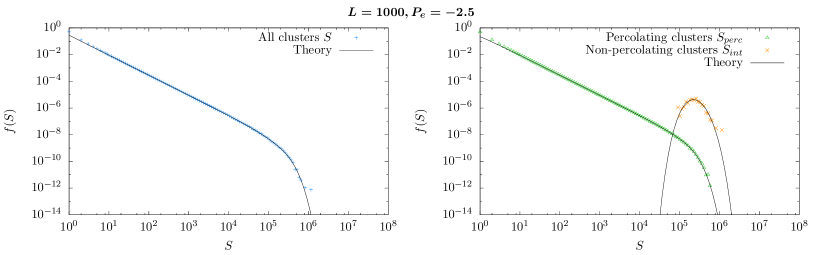
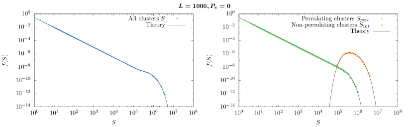
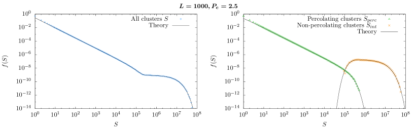
Figure 2: Distribution of sizes in the geometric Galton-Watson process in the three regimes: subcritical ($P_{e}=-2.5$, top), critical ($P_{e}=0$, middle), and supercritical ($P_{e}=2.5$, bottom), together with theoretical predictions from the first-passage times of a diffusion process (numerical inversion of the Laplace transform is done by the Talbot method using the routine in Ref. Laplace_inversion ). Plots on the left show the full distribution. Plots on the right show the distribution decomposed into its percolating and non-percolating contributions. In the critical regime, the complete distribution $f(S)$ (middle left) shows a small bump for large sizes, which is much more pronounced in the supercritical regime. The subcritical distribution, having no bump (top left), can be visually confused with a critical distribution. Logarithmic binning has been applied Christensen_Moloney ; Corral_Deluca .

A numerical inversion of $f_{0}(s)$ is shown in Fig. 2.

The first two moments can be similarly expanded as

$$\langle t_{0}\rangle =\frac{1}{2P_{e}\tanh P_{e}}\left(1+P_{e}\tanh P_{e}-\frac{P_{e}}{\tanh P_{e}}\right)\tau{u_{0}}+\mathcal{O}({u_{0}}^{2}),$$ (10)

$$\langle t_{0}^{2}\rangle =\frac{1}{2P_{e}^{3}\tanh P_{e}}\left(\frac{1}{2}-\frac{P_{e}\tanh P_{e}}{2}+\frac{P_{e}}{2\tanh P_{e}}+P_{e}^{2}-\frac{P_{e}^{2}}{\tanh^{2}P_{e}}\right){\tau^{2}{u_{0}}}+\mathcal{O}({u_{0}}^{2}).$$ (11)

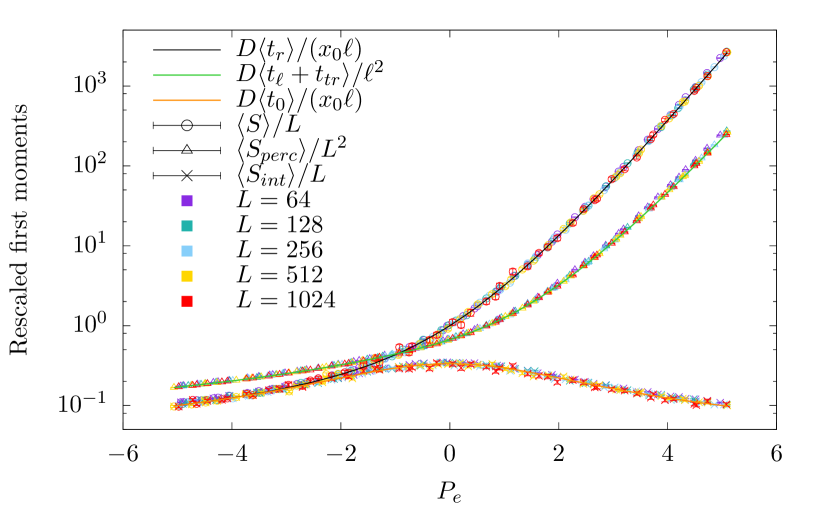
Figure 3: Rescaled mean sizes (simulations, $10^{5}$ realizations) and rescaled times (theory) versus Péclet number for different systems sizes $L$.

A plot of $\langle t_{0}\rangle$ as a function of $P_{e}$ is shown in Fig. 3.

Note that these expressions are even in $P_{e}$. The expansions are valid in the limit of small $u_{0}$, i.e., $x_{0}\ll\ell$ (more precisely, $u_{0}P_{e}\ll 1$ and $u_{0}R\ll 1$). See Eqs. (45), (46), and (47) in Appendix A for their full derivation.

II.3 Critical point

The critical point corresponds to diffusion with no drift, $P_{e}=0$ (i.e. $v=0$). Using the results of Appendix A, the exact distribution reads

$$f_{0}^{*}(s)=\frac{\sinh[(1-u_{0})\sqrt{\tau s}]}{(1-u_{0})\sinh\sqrt{\tau s}},$$

where the asterisk denotes the critical point. To first order in $u_{0}$

$$f_{0}^{*}(s)=1-\left(\frac{\sqrt{\tau s}}{\tanh\sqrt{\tau s}}-1\right)u_{0}+\mathcal{O}({u_{0}}^{2}).$$ (12)

Figure 2 shows a plot of the numerical inverse Laplace transform of $f_{0}^{*}(s)$. The case $P_{e}=0$ and $\ell$ infinite corresponds to $\tau s\gg 1$, for which

$$f_{0}^{*}(s)=j_{0}^{*}(s)\simeq 1-{{u_{0}}\sqrt{\tau s}}+\mathcal{O}({u_{0}}^{2}).$$

After inverting the Laplace transform (see e.g. Eq. 4.6.23 of Ref. Bleistein ),

$$f_{0}^{*}(t)=j_{0}^{*}(t)\simeq\frac{{u_{0}}}{2}\sqrt{\frac{\tau}{\pi t^{3}}}+\mathcal{O}({u_{0}}^{2}),$$ (13)

for $P_{e}=0$ and $t\ll\tau=\ell^{2}/D$, thereby recovering the well-known $t^{-3/2}$ behavior of first-passage to the origin in an infinite system.

To lowest order in $u_{0}$, the moments are given by

$$\langle t_{0}^{*}\rangle =\frac{\tau{u_{0}}}{3}=\frac{x_{0}\ell}{3D},$$ (14)

$$\sigma_{0}^{*}\simeq\sqrt{\langle t_{0}^{2*}\rangle} =\sqrt{\frac{2\tau^{2}{u_{0}}}{45}}=\sqrt{\frac{2x_{0}\ell^{3}}{45D^{2}}},$$ (15)

expanding Eq. (12) for small $\sqrt{\tau s}=\ell\sqrt{s/D}$.

II.4 Absorbing boundary at $x=\ell$ and splitting probability

Although already studied in Ref. Font_clos_molon , for completeness we summarize the results for absorption at $x=\ell$. In the notation of this article, we extract from Eq. (8) the expansion

$$j_{\ell}(s)=-Dc^{\prime}(x=\ell,s)=\frac{e^{(1-{u_{0}})P_{e}}\sinh({u_{0}}R)}{\sinh R}=\frac{e^{P_{e}}R{u_{0}}}{\sinh R}+\mathcal{O}({u_{0}}^{2}),$$ (16)

valid for $u_{0}\ll 1$. For $z=\tau s/P_{e}^{2}\ll 1$,

$$j_{\ell}(s)=\frac{e^{P_{e}}P_{e}{u_{0}}}{\sinh P_{e}}\left[1-\left(-1+\frac{P_{e}}{\tanh P_{e}}\right)\frac{z}{2}+\frac{1}{2}\left(\frac{2P_{e}^{2}}{\tanh^{2}P_{e}}-\frac{P_{e}}{\tanh P_{e}}-P_{e}^{2}-1\right)\frac{z^{2}}{4}+\mathcal{O}(z^{3})\right]+\mathcal{O}({u_{0}}^{2}),$$ (17)

So, to zeroth order in ${u_{0}}$,

$$\langle t_{\ell}\rangle =\frac{\tau}{2P_{e}^{2}}\left(\frac{P_{e}}{\tanh P_{e}}-1\right)+\mathcal{O}({u_{0}}),$$ (18)

$$\langle t_{\ell}^{2}\rangle =\frac{\tau^{2}}{4P_{e}^{4}}\left(\frac{2P_{e}^{2}}{\tanh^{2}P_{e}}-\frac{P_{e}}{\tanh P_{e}}-P_{e}^{2}-1\right)+\mathcal{O}({u_{0}}).$$ (19)

Note that the common multiplying factor in Eq. (17),

$$C_{\ell}=j_{\ell}(0)=\frac{e^{(1-{u_{0}})P_{e}}\sinh({u_{0}}P_{e})}{\sinh P_{e}}=\frac{e^{P_{e}}P_{e}{u_{0}}}{\sinh P_{e}}+\mathcal{O}({u_{0}}^{2}).$$ (20)

gives the ratio between the outflux of particles at $\ell$, denoted by $j_{\ell}(t)$, and the probability density $f_{\ell}(t)$ of the first-passage time to the boundary at $x=\ell$; i.e., $j_{\ell}(t)=C_{\ell}f_{\ell}(t)$, so that,

$$f_{\ell}(s)=\frac{j_{\ell}(s)}{C_{\ell}}=\frac{\sinh P_{e}}{\sinh R}\frac{\sinh(u_{0}R)}{\sinh(u_{0}P_{e})}=\frac{R\sinh P_{e}}{P_{e}\sinh R}+\mathcal{O}(u_{0}).$$

$C_{\ell}$ is known as the splitting probability Redner ; Farkas . Note that $\langle t_{\ell}\rangle$, $\langle t_{\ell}^{2}\rangle$, and $f_{\ell}(s)$ (and therefore $f_{\ell}(t)$) are even for $P_{e}$ (but not $j_{\ell}(s)$ and $C_{\ell}$). For $P_{e}=0$ (i.e., at the critical point) one has that $f_{\ell}^{*}(s)$, to first order in $u_{0}$, is the Laplace transform of the celebrated Kolmogorov-Smirnov distribution Botet ; Font_clos_molon ,

$$f_{\ell}^{*}(s)=\frac{\sinh(u_{0}\sqrt{\tau s})}{u_{0}\sinh\sqrt{\tau s}}=\frac{\sqrt{\tau s}}{\sinh\sqrt{\tau s}}+\mathcal{O}({u_{0}}).$$ (21)

The factor $C_{\ell}$ is also the probability that a particle is absorbed at $x=\ell$. Equation (20) is the same scaling law found in Refs. GarciaMillan ; Corral_garciamillan , as explained in the next section. A formula for $C_{\ell}$ also appears in Refs. Redner ; Farkas ; Font_clos_molon , but without expanding in ${u_{0}}$, therefore hiding its finite-size scaling. The probability that a particle is instead absorbed at $x=0$ is $C_{0}=1-C_{\ell}\simeq 1$ (to zeroth order in $u_{0}$).

Combining the results for $t_{\ell}$ with those obtained previously for $t_{0}$, we have the solution of one-dimensional diffusion between two absorbing boundaries. In Appendix B, we show that it displays a phase transition with finite-size scaling when $x_{0}\ll\ell$ Farkas .

II.5 Reflecting boundary at $x=\ell$

We now consider first-passage times to $x=0$, starting from a reflecting boundary at $x=\ell$. The initial condition is most conveniently handled by injecting into an empty interval a single particle at $x=\ell$. Together with a zero flux condition at this boundary for $t>0$, this stipulates that

$$j_{tr\ell}(t)=\left[vc(x,t)-D\frac{\partial c(x,t)}{\partial x}\right]_{x=\ell}=-\delta(t),$$

where the $-\delta(t)$ term ensures that the injection (hence minus sign) occurs at $t=0$. In Laplace space, this boundary condition reads

$$vc(x=\ell,s)-D{c^{\prime}(x=\ell,s)}=-1.$$

Note that in this case there is no dependence on $u_{0}$, since the particle is injected precisely at $x=\ell$. The absorbing boundary condition at $x=0$ remains unchanged.

The solution of the diffusion equation (Eq. (2)) with these boundary conditions is provided in detail in Refs. Redner and Font_clos_molon . The outflux at the absorbing boundary is

$$f_{tr}(s)=j_{tr0}(s)=Dc^{\prime}(x=0,s)=\frac{e^{-P_{e}}R}{R\cosh R-P_{e}\sinh R},$$ (22)

where the subscript $tr$ denotes transmission from the reflecting to the absorbing boundary Redner . In contrast to the case of two absorbing boundaries, this Laplace transform is not even in $P_{e}$. The exact moments are given by

$$\langle t_{tr}\rangle =\frac{\tau}{4P_{e}^{2}}(e^{2P_{e}}-2P_{e}-1),$$ (23)

$$\langle t_{tr}^{2}\rangle =\frac{\tau^{2}}{8P_{e}^{4}}[e^{4P_{e}}+(1-6P_{e})e^{2P_{e}}+2(P_{e}^{2}-1)],$$ (24)

see Ref. Redner . For the critical case ($P_{e}=0$), we recover

$$f_{tr}^{*}(s)=j_{tr}^{*}(s)=\frac{1}{\cosh\sqrt{\tau s}}$$

as in Ref. Font_clos_molon .

Since $t_{\ell}$ and $t_{tr}$ are independent random variables, the total time $t_{\ell tr}=t_{\ell}+t_{tr}$ until absorption, having first reached $x=\ell$ from the origin, Laplace transforms as Font_clos_molon

$$f_{\ell tr}(s)=f_{\ell}(s)f_{tr}(s)=\frac{R^{2}e^{-P_{e}}\sinh P_{e}}{P_{e}R\sinh R\cosh R-P_{e}^{2}\sinh^{2}R}+\mathcal{O}(u_{0}).$$ (25)

$\langle t_{\ell tr}\rangle$ and the inverse Laplace transforms of $f_{\ell tr}(s)$ and $f_{\ell tr}^{*}(s)$ are shown in Figs. 3 and 2.

II.6 Entire diffusion problem: moments

We are now in a position to study the entire diffusion problem. The quantity of primary interest is the first-passage time to $x=0$, denoted $t_{r}$, where the subscript $r$ refers to the so-called reflection mode Redner . This time is a mixture of two times: $t_{0}$ (for realizations that do not reach $x=\ell$ before absorption at $x=0$), and $t_{\ell tr}=t_{\ell}+t_{tr}$ (for realizations that do reach $x=\ell$ before absorption at $x=0$). The weight of each time is given by $1$ (to zeroth order in $u_{0}$) and $C_{\ell}$ (from Eq. (20)), respectively. Thus, to lowest order in $u_{0}$, the expected value of $t_{r}$ is

$$\langle t_{r}\rangle =\langle t_{0}\rangle+C_{\ell}{\left(\langle t_{\ell}\rangle+\langle t_{tr}\rangle\right)}$$

$$=\left\{\frac{1}{2P_{e}\tanh P_{e}}\left(1+P_{e}\tanh P_{e}-\frac{P_{e}}{\tanh P_{e}}\right)\right.$$

$$+\left.\frac{e^{P_{e}}P_{e}}{\sinh P_{e}}\left[\frac{1}{2P_{e}^{2}}\left(\frac{P_{e}}{\tanh P_{e}}-1\right)+\frac{e^{2P_{e}}-2P_{e}-1}{4P_{e}^{2}}\right]\right\}\tau{u_{0}}+\mathcal{O}({u_{0}}^{2}),$$ (26)

which is plotted in Fig. 3.

For the second moment we find

$$\langle t_{r}^{2}\rangle=\langle t_{0}^{2}\rangle+C_{\ell}{\left(\langle t_{\ell}^{2}\rangle+\langle t_{tr}^{2}\rangle+2\langle t_{\ell}\rangle\langle t_{tr}\rangle\right)},$$ (27)

to lowest order in $u_{0}$. This result is due to the fact that the moments of any order (with respect to the origin $t=0$) are additive in a mixture of random variables (including the corresponding weights), but not for the sum of independent random variables ($t_{\ell}$ and $t_{tr}$), for which only the variances are additive. The particular form of $\langle t_{r}^{2}\rangle$ can be obtained directly from Eqs. (11), (19), and (24). To first order in $u_{0}$, $\sigma_{r}^{2}=\langle t_{r}^{2}\rangle$.

II.7 Possible order parameters

Asymptotically, the first moment of $t_{r}$, Eq. (26), behaves as

$$\langle t_{r}\rangle \sim\langle t_{0}\rangle\sim\frac{\tau u_{0}}{2|P_{e}|}=\frac{x_{0}}{|v|} \qquad\mbox{ for }P_{e}\rightarrow-\infty,$$

$$\langle t_{r}^{*}\rangle =\left[\frac{1}{3}+1\cdot\left(\frac{1}{6}+\frac{1}{2}\right)\right]\tau u_{0}=\frac{\ell x_{0}}{D} \qquad\mbox{ for }P_{e}=0,$$

$$\langle t_{r}\rangle \sim C_{\ell}\langle t_{tr}\rangle\sim\frac{\tau u_{0}e^{2P_{e}}}{2P_{e}}=\frac{x_{0}e^{\ell v/D}}{v} \qquad\mbox{ for }P_{e}\rightarrow\infty.$$

as obtained immediately from Eqs. (10), (18), (20), and (23). On the other hand, the order parameter considered in Refs. Font_clos_molon ; Botet , $t_{\ell tr}=t_{\ell}+t_{tr}$, behaves as

$$\langle t_{\ell tr}\rangle \sim\frac{\tau}{|P_{e}|}=\frac{2\ell}{|v|} \qquad\mbox{ for }P_{e}\rightarrow-\infty,$$

$$\langle t_{\ell tr}^{*}\rangle =\left(\frac{1}{6}+\frac{1}{2}\right)\tau=\frac{2\ell^{2}}{3D} \qquad\mbox{ for }P_{e}=0,$$

$$\langle t_{\ell tr}\rangle \sim\langle t_{tr}\rangle\sim\frac{\tau e^{2P_{e}}}{4P_{e}^{2}}=\frac{De^{\ell v/D}}{v^{2}} \qquad\mbox{ for }P_{e}\rightarrow\infty,$$

Finally, the order parameter of Refs. GarciaMillan ; Corral_garciamillan behaves as

$$C_{\ell} \sim 2u_{0}{|P_{e}|}e^{-2|P_{e}|}=\frac{x_{0}|v|}{D}e^{-\ell|v|/D} \qquad\mbox{ for }P_{e}\rightarrow-\infty,$$

$$C_{\ell}^{*} =u_{0}=\frac{x_{0}}{\ell} \qquad\mbox{ for }P_{e}=0,$$

$$C_{\ell} \sim 2u_{0}P_{e}=\frac{x_{0}v}{D} \qquad\mbox{ for }P_{e}\rightarrow\infty.$$

All three quantities, $\langle t_{r}\rangle$, $\langle t_{\ell tr}\rangle$, and $C_{\ell}$, are reasonable candidates for order parameters — finding the order parameter of a phase transition is often not obvious Fisher_school : citing J. P. Sethna, “there is often more than one sensible choice” Sethna_book .

Typically, one expects that in the thermodynamic limit ($\ell\rightarrow\infty$) the order parameter goes to zero for $P_{e}<0$ and scales with a power of $\ell$ for $P_{e}>0$ (if the order parameter is extensive). This is not the case for $\langle t_{r}\rangle$ or $\langle t_{\ell tr}\rangle$, and there is no simple rescaling to bring about the desired behavior. Instead, one could redefine the order parameters somewhat artificially as $\ell^{-1}\ln(|v|\langle t_{r}\rangle/x_{0})$ and $\ell^{-1}\ln(v^{2}\langle t_{\ell tr}\rangle/D)$, which below and above the critical point behave as intensive order parameters — but they are not well defined at the critical point. $C_{\ell}$, meanwhile, undergoes a transcritical bifurcation at the critical point Corral_Alseda_Sardanyes , but below the transition it goes to zero exponentially rather than as a power law of $1/\ell$. A drawback of all three order parameters is the lack of an associated variance that diverges at the critical point.

II.8 Finite-size scaling for the moments of the distributions

The equations in the previous subsections show that, when $u_{0}$ is small, all the first-passage times ($t_{0},t_{\ell},t_{tr},t_{\ell tr}$, and $t_{r}$) obey finite-size scaling laws Privman . Indeed, starting with $t_{\ell}$,

$$\langle t_{\ell}\rangle ={\tau}G_{\ell 1}\left(P_{e}\right)=\frac{\ell^{2}}{D}G_{\ell 1}\left(\frac{\ell v}{2D}\right),$$

$${\langle t_{\ell}^{2}\rangle} =\tau^{2}G_{\ell 2}\left(P_{e}\right)=\frac{\ell^{4}}{D^{2}}G_{\ell 2}\left(\frac{\ell v}{2D}\right),$$

to zeroth order in $u_{0}$, where $G_{\ell 1}(P_{e})$ and $G_{\ell 2}(P_{e})$ are scaling functions completely determined by Eqs. (18) and (19). The same scaling holds for $t_{tr}$ and $t_{\ell tr}$ (but with different scaling functions). In contrast, from Eqs. (26) and (27),

$$\langle t_{r}\rangle ={{u_{0}}\tau}G_{r1}\left(P_{e}\right)=\frac{x_{0}\ell}{D}G_{r1}\left(\frac{\ell v}{2D}\right),$$ (28)

$${\langle t_{r}^{2}\rangle} ={u_{0}}\tau^{2}G_{r2}\left(P_{e}\right)=\frac{x_{0}\ell^{3}}{D^{2}}G_{r2}\left(\frac{\ell v}{2D}\right),$$ (29)

to first order in $u_{0}$. The moments of $t_{0}$ share the same scaling (but with different scaling functions). For further comparison,

$$C_{\ell}=u_{0}G_{c}\left(P_{e}\right)=\frac{x_{0}}{\ell}G_{c}\left(\frac{\ell v}{2D}\right),$$

to lowest order in $u_{0}$. Note that the position of the critical point does not shift with $\ell$: it remains at $P_{e}=0$ (or $v=0$) for finite $\ell$.

II.9 Entire diffusion problem: distribution

The Laplace transform of the probability density of the first-passage time, $t_{r}$, can be written as the weighted sum

$$f_{r}(s)=(1-C_{\ell})f_{0}(s)+C_{\ell}f_{\ell}(s)f_{tr}(s)=j_{0}(s)+j_{\ell}(s)f_{tr}(s).$$

From Eqs. (42), (16), and (22), we thus obtain

$$f_{r}(s)=j_{0}(s)+j_{\ell}(s)f_{tr}(s)=\frac{e^{-P_{e}u_{0}}\sinh[(1-u_{0})R]}{\sinh R}+\frac{2e^{-u_{0}P_{e}}R\sinh(u_{0}R)}{R\sinh(2R)-2P_{e}\sinh^{2}R},$$

which, at the critical point $P_{e}=0$, reduces to

$$f_{r}^{*}(s)=\frac{\sinh[(1-u_{0})\sqrt{\tau s}]}{\sinh\sqrt{\tau s}}+\frac{2\sinh(u_{0}\sqrt{\tau s})}{\sinh(2\sqrt{\tau s})}.$$

Expanding in $u_{0}$, we find (see Eqs. (43), (16), and (22))

$$f_{r}(s) =1-\left(P_{e}+\frac{R}{\tanh R}\right){u_{0}}+\left(\frac{e^{P_{e}}R}{\sinh R}\right)\left(\frac{e^{-P_{e}}R}{R\cosh R-P_{e}\sinh R}\right){u_{0}}+\mathcal{O}({u_{0}}^{2})$$

$$=1-\left(P_{e}+\frac{R}{\tanh R}-\frac{2R^{2}}{R\sinh(2R)-2P_{e}\sinh^{2}R}\right){u_{0}}+\mathcal{O}({u_{0}}^{2}),$$ (30)

valid for $u_{0}R\ll 1$. At the critical point ($P_{e}=0$),

$$f_{r}^{*}(s) =1-\frac{\sqrt{\tau s}}{\tanh\sqrt{\tau s}}u_{0}+\left(\frac{\sqrt{\tau s}}{\sinh\sqrt{\tau s}}\right)\left(\frac{1}{\cosh\sqrt{\tau s}}\right)u_{0}+\mathcal{O}(u_{0}^{2})$$

$$=1-\left(\frac{\sqrt{\tau s}}{\tanh\sqrt{\tau s}}-\frac{\sqrt{4\tau s}}{\sinh\sqrt{4\tau s}}\right)u_{0}+\mathcal{O}(u_{0}^{2}).$$

Plots of the inverse Laplace transforms of $f_{r}(s)$ and $f_{r}^{*}(s)$ are shown in Fig. 2. Note that all the results presented here for diffusion processes are valid for $x_{0}\ll\ell$.

II.10 Finite-size scaling for the distributions

The Laplace transforms of the probability densities of $t_{\ell}$, $t_{tr}$, and $t_{\ell tr}$ obey simple finite-size scaling laws (to zeroth order in $u_{0}$),

$$f_{\ell}(s)=\hat{F}_{\ell}\left(\tau s,P_{e}\right)=\hat{F}_{\ell}\left(\frac{\ell^{2}s}{D},\frac{\ell v}{2D}\right),$$ (31)

from Eq. (21), where the scaling function $\hat{F}_{\ell}$ is exactly known. Again, $f_{tr}(s)$ and $f_{\ell tr}(s)$ scale in the same way as $f_{\ell}(s)$ (with different scaling functions). Inverting the Laplace transforms, we see that the probability densities also obey simple finite-size scaling laws for fixed $P_{e}$,

$$f_{\ell}(t)=\frac{1}{\tau}F_{\ell}\left(\frac{t}{\tau},P_{e}\right)=\frac{D}{\ell^{2}}F_{\ell}\left(\frac{Dt}{\ell^{2}},\frac{\ell v}{2D}\right),$$ (32)

with $f_{tr}(t)$ and $f_{\ell tr}(t)$ scaling in the same way.

In contrast, the Laplace transforms associated with $t_{r}$ and $t_{0}$ obey

$$f_{r}(s)=\hat{F}_{r}\left(\tau s,{u_{0}},P_{e}\right)=\hat{F}_{r}\left(\frac{\ell^{2}s}{D},\frac{x_{0}}{\ell},\frac{\ell v}{2D}\right),$$ (33)

to first order in $u_{0}$, from Eq. (30). This is not finite-size scaling for fixed $x_{0}$, due to the dependence on $u_{0}$; $f_{0}$ obeys an analogous equation. The corresponding densities obey

$$f_{r}(t)=\frac{1}{\tau}F_{r}\left(\frac{t}{\tau},{{u_{0}}},P_{e}\right)=\frac{D}{\ell^{2}}F_{r}\left(\frac{Dt}{\ell^{2}},\frac{x_{0}}{\ell},\frac{\ell v}{2D}\right),$$ (34)

with $f_{0}(t)$ scaling in the same way, but with its own scaling function. However, as the moments of $t_{r}$ and $t_{0}$ have an extra factor $u_{0}$ in comparison with $t_{\ell}$ and $t_{tr}$, this suggests that the densities and their transforms can be written with an extra factor $u_{0}$ as well, i.e.,

$$f_{r}(t)=\frac{u_{0}}{\tau}F_{r}\left(\frac{t}{\tau},P_{e}\right)=\frac{Dx_{0}}{\ell^{3}}F_{r}\left(\frac{Dt}{\ell^{2}},\frac{\ell v}{2D}\right),$$ (35)

where in a slight abuse of notation we have recycled the symbol $F_{r}$, which now refers to a different scaling function. $t_{0}$ obeys an analogous equation (now truly a finite-size scaling law). The scaling law for $f_{r}(t)$ is compatible with the form

$$f_{r}(t)=\frac{1}{m}\left(\frac{m}{t}\right)^{\alpha}F\left(\frac{t}{\tau},P_{e}\right)$$ (36)

(and similarly for $f_{0}(t)$) with the new scaling function $F$ going to a constant for small arguments and decaying very fast for large arguments, and with $\alpha=3/2$ and $m={u_{0}}^{2}\tau$ the minimum value of $t$ (that is, for $t<m$ the probability density $f_{0}(t)$ can be considered as zero). This is in agreement with the power-law behavior shown in Eq. (13). An alternative way to write the scaling law (36) is:

$$f_{r}(t)=\frac{1}{m}\left(\frac{m}{\tau}\right)^{\alpha}\tilde{F}\left(\frac{t}{\tau},P_{e}\right)$$ (37)

with the scaling function $\tilde{F}$ absorbing the power-law part with exponent $\alpha=3/2$. For $P_{e}=0$ this leads to the same scaling law as in Ref. Corral_csf . In fact, that reference gives a more direct derivation of the scaling laws (36) and (37), but only for $f_{0}(t)$ with $P_{e}=0$.

III Branching process and size distributions

III.1 Diffusion and random walks

First, we recall the connection between diffusion and random walks. Consider a random walk described by a position $X$ at time $T$, which are both discrete and dimensionless. At each time step $T$, the position $X$ increases by one unit with probability $q$, or decreases by one unit with probability $1-q$. The continuum limit of the random walk is a diffusion process, with $x=X\delta_{x}$ and $t=T\delta_{t}$, where $\delta_{x}$ and $\delta_{t}$ are elementary space and time units, which tend to zero Redner . The limiting process is described by the diffusion equation, Eq. (1), with $v=(2q-1)\delta_{x}/\delta_{t}$ and $D=2q(1-q)\delta_{x}^{2}/\delta_{t}$. In this limit, the results obtained for moments and probability densities of diffusion processes are also valid for random walks Redner . As all the relevant equations of the previous section can be written in terms of dimensionless quantities, we can make the substitutions

$$v\rightarrow 2\left(q-\frac{1}{2}\right),\hskip 28.45274ptD\rightarrow 2q(1-q),\hskip 28.45274pt\mbox{and}\hskip 28.45274pt\tau\rightarrow\frac{L^{2}}{2q(1-q)},$$ (38)

together with $u_{0}=X_{0}/L$, with $X_{0}=x_{0}/\delta_{x}$ and $L=\ell/\delta_{x}$; in particular

$$P_{e}=\frac{L(q-1/2)}{2q(1-q)}.$$ (39)

As an illustration, Eq. (26) becomes

$$\langle T_{r}\rangle=\frac{1}{4P_{e}}\left(\frac{e^{3P_{e}}}{\sinh{P_{e}}}-\frac{1}{\tanh P_{e}}-3\right)\frac{X_{0}L}{2q(1-q)}+\mathcal{O}(u_{0}^{2}).$$ (40)

Care is required approximating the (dimensionless) probability mass functions of random walk times $T$, with the probability densities for diffusion times $t$, which have the dimensions of time^-1. Note that, in the former case, first-passage times are discretized in steps of 2 (since boundaries can only be reached in either an odd or even number of steps). Thus, the two functions are related via

$$f_{T}(T)=2\delta_{t}f_{t}(T\delta_{t}),$$ (41)

where $f_{T}$ denotes the probability mass function for the random walk and $f_{t}$ the probability density for the diffusion process. The extra factor 2 with respect a standard change of variables comes from the discretization of $T$. In this way, rewriting Eqs. (32) and (35) for random walk scaling laws, we obtain

$$f_{L}(T)=\frac{4q(1-q)}{L^{2}}F_{\ell}\left(\frac{2q(1-q)T}{L^{2}},P_{e}\right)\simeq\frac{1}{L^{2}}F_{\ell}\left(\frac{T}{2L^{2}},P_{e}\right),$$

with an analogous expression for $f_{TR}(T)$, while

$$f_{R}(T)=\frac{4q(1-q)X_{0}}{L^{3}}F_{r}\left(\frac{2q(1-q)T}{L^{2}},P_{e}\right)\simeq\frac{X_{0}}{L^{3}}F_{r}\left(\frac{T}{2L^{2}},P_{e}\right),$$

where we have used $q\simeq 1/2$ close to the critical point. The scaling functions $F_{\ell}$ and $F_{r}$ are the same as for the diffusion process of the previous section.

III.2 Branching processes

We now consider the Galton-Watson branching process associated with the random walk. The branching process starts with one single member (also known as the root), defining the first generation. It produces a random number of offspring drawn from a geometric distribution, i.e. the probability of $k$ offspring is $(1-q)q^{k}$, $k=0,1,2,\ldots$, where $1-q$ is the success probability. Each of these second generation offspring produce their own (third generation) offspring, and so on, independently and identically. The process can be visualised as a rooted tree. In principle, $q$ is the only parameter of the model, but one can introduce finite-size effects by stopping the branching process at generation $L$.

The size $S$ of the branching process, or the size of the tree or cluster, is given by its total population (total number of offspring plus root, or, equivalently, the total number of vertices in the tree) Harris_original ; Corral_FontClos . In a finite system, clusters can be classified into two types: percolating clusters, which reach generation $L$, and non-percolating clusters, which do not. We denote the size of each of these by the random variables $S_{perc}$ (for percolating) and $S_{int}$ (internal, for non-percolating). Overall, $S$ is a mixture of $S_{perc}$ and $S_{int}$.

III.3 Mapping from branching processes to random walks

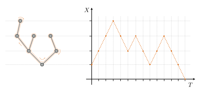
Figure 4: Correspondence between trees and positive walks (excursions), known as a Harris walk Harris52 . A walker starts at the root of the tree (the vertex at the bottom) and follows each branch in turn to its end, starting with the left-most branch. If the tree is generated from a geometric offspring distribution, the resulting path is a simple random walk.

Harris’ mapping from trees to walks proceeds as follows (for complete details see Refs. Harris52 ; Font_clos_molon ; Corral_garciamillan ; Devroye_notes , for a visual explanation, see Fig. 4). A (deterministic) walker is placed at the root of the tree and carries out a so-called depth-first search by traversing each branch in turn to its very end, starting with the leftmost branch. Whenever a choice of unvisited branches presents itself, the walker traverses them in the order left to right. Eventually, the walker will return to the root, having traversed all branches. In doing so, the walker will have visited each member of the tree twice. To define a positive walk, it is convenient to append a final step to a “generation zero”, see Fig. 4. In this way, one obtains a one-dimensional, positive walk (or excursion), starting at $X=1$ and ending at $X=0$, where $X$ corresponds to the generation number as the walker traverses the tree. The size of the tree $S$ is then seen to be the duration of the walk (plus one) divided by two — the division by two takes care of the fact that each member of the tree is visited twice.

In addition, a probability measure over the set of all positive walks is inherited from the probability measure over the set of rooted trees. When the tree is generated with a geometric offspring distribution with success probability $p$, one obtains the standard random walk, where $X\rightarrow X+1$ with probability $q=1-p$, and $X\rightarrow X-1$ with probability $p$.

In this way, a realization of a Galton-Watson process with geometric offspring distribution is equivalent to a realization of a random walk that starts at $X=1$ and ends at $X=0$, staying positive in between. The stipulation that a branching process cannot exceed $L$ generations is effected, in the random walk, by a reflecting boundary at $X=L$.

III.4 Moments and splitting probability

One can calculate $S_{perc}$ from the first-passage time of a diffusing particle that first reaches $x=\ell$, before being absorbed at $x=0$ (as in Ref. Font_clos_molon ). The total time is the sum of two independent times: the first, $t_{\ell}$, is the time to reach $x=\ell$ starting from $x=x_{0}$ (and not touch $x=0$), and the second, $t_{tr}$, is the time to reach $x=0$ starting from $x=\ell$, see Ref. Font_clos_molon . Thus, in terms of a random walk, $S_{perc}=(T_{L}+T_{tr}+1)/2$, where the discrete and dimensionless times $T_{L}$ and $T_{tr}$ are analogs of $t_{\ell}$ and $t_{tr}$ for the diffusion process. Similarly, $S_{int}$ is obtained from the first-passage time to $x=0$ of a diffusing particle that does not reach $x=\ell$, denoted $t_{0}$. Thus, $S_{int}=(T_{0}+1)/2$, with $T_{0}=t_{0}/\delta_{t}$. The total size $S$ (percolating or not) can be obtained directly from the total first-passage time $t_{r}$, via $S={(T_{r}+1)}/2,$ with $T_{r}=t_{r}/\delta_{t}$. The moments of $S$ are

$$\langle S\rangle =\frac{\langle T_{r}\rangle+1}{2}\simeq\frac{\langle t_{r}\rangle}{2\delta_{t}},$$

$$\langle S^{2}\rangle =\frac{\langle T_{r}^{2}\rangle+2\langle T_{r}\rangle+1}{4}\simeq\frac{\langle t_{r}^{2}\rangle}{4\delta_{t}^{2}},$$

for $L\gg 1$. Thus, from Eq. (40)

$$\langle S\rangle=\frac{1}{8P_{e}}\left(\frac{e^{3P_{e}}}{\sinh{P_{e}}}-\frac{1}{\tanh P_{e}}-3\right){2L}+\frac{1}{2},$$

where we have used the fact that, close to the critical point, $q\simeq 0.5$. In the limit of large system size, the moments of $S$ obey the same scaling laws as those of $t_{r}$, Eqs. (28) and (29), i.e.

$$\langle S\rangle=\frac{L}{4q(1-q)}G_{r1}\left(\frac{L(q-1/2)}{2q(1-q)}\right)\simeq{L}G_{r1}\left({2L(q-1/2)}\right),$$

Figure 3 shows good agreement between theory and realizations of branching processes from computer simulations.

Note that the scaling law for $C_{\ell}$, Eq. (20), derived in the diffusion framework, is the same as that obtained for branching processes in Refs. GarciaMillan ; Corral_garciamillan . Indeed, transcribing $\ell$, $D$ and $v$ into their discrete versions, Eq. (38), we get

$$2P_{e}=\frac{\ell v}{D}\simeq 4L\left(q-\frac{1}{2}\right)\simeq L(\langle k\rangle-1)$$

to first order in $q-1/2$, with $\langle k\rangle=q/p\simeq 1+4(q-1/2)$ for the geometric distribution. Substituting the previous expression for $2P_{e}$ into Eq. (20), with $x_{0}/\ell=1/L$, leads to the result of Refs. GarciaMillan ; Corral_garciamillan .

III.5 Distribution of sizes

The distributions of sizes $f_{S}(S)$ (for $S_{int},S_{perc}$ or total $S$) are related to the distributions of first-passage times in the random walk $f_{T}(T)$ and in the diffusion process $f_{t}(t)$ via

$$f_{S}(S)=f_{T}(2S-1)=2\delta_{t}f_{t}((2S-1)\delta_{t}),$$

using Eq. (41). While we do not have explicit formulas for $f_{T}(T)$ and $f_{t}(t)$, we do have their Laplace transforms $f_{t}(s)$. Thus, given a finite-size Galton-Watson branching process, with parameters $q$ and $L$, we can calculate $\tau$, $P_{e}$, and $u_{0}$ for the equivalent diffusion process, using Eqs. (38) and (39), and then perform the numerical inversion of the Laplace-transformed expressions (9), (25), and (30). This yields a nearly perfect agreement between computer simulations of the Galton-Watson process and theory, based on diffusion processes, as Fig. 2 illustrates.

Note from the figure that the critical case, $P_{e}=0$, displays a bump before the exponential decay at large sizes, which comes from the Kolmogorov-Smirnov distribution associated with percolating clusters. Similar bumps have been observed in paradigmatic models of critical phenomena, such as the Oslo sandpile model Corral_thesis . Therefore, although deviations from criticality ($P_{e}\neq 0$) in infinite systems lead to a $f(S)$ given by a power-law multiplied by an exponential tail ($f(S)\propto e^{-S/\xi}/S^{3/2}$, see Ref. Corral_FontClos ), this parameterization is not valid for finite-size effects at the critical point, since it does not reproduce the bump for large $S$. A much larger bump is present in the supercritical regime.

This behavior can be taken as an instance of the so-called dragon-king effect Sornette_dragon_king , in which events at the tail of a distribution have a much larger probability than that given by the extrapolation of a power-law central part. This would correspond to the so-called characteristic-earthquake scenario in statistical seismology Ben_Zion_review , although from our results and those of Ref. Font_clos_molon it seems clear that the bump cannot be described by Gaussian-like statistics (which is only applicable in the subcritical regime, where the bump is negligible or very small, depending on $P_{e}$), contrary to the statement in Ref. Ben_Zion_review .

Finally, from Eqs. (32) and (35), the scaling laws for the size distributions can be written as

$$f_{perc}(S) =\frac{1}{L^{2}}F_{\ell tr}\left(\frac{2S-1}{2L^{2}},P_{e}\right),$$

$$f_{int}(S) =\frac{1}{L^{3}}F_{0}\left(\frac{2S-1}{2L^{2}},P_{e}\right),$$

$$f(S) =\frac{1}{L^{3}}F_{r}\left(\frac{2S-1}{2L^{2}},P_{e}\right),$$

where, again, $q\simeq 1/2$ close the the critical point. The scaling functions $F_{\ell}$, $F_{0}$, and $F_{r}$ are the same as for the diffusion process.

IV Summary and Conclusions

The Harris walk mapping establishes a direct correspondence between finite-size branching processes (in which the number of generations cannot exceed $L$) and one-dimensional random walks between $X=0$ and $X=L$. By approximating random walks with diffusions, techniques from the latter can be applied to branching processes, such that first-passage times of Brownian particles with drift correspond to sizes of trees generated by the branching process (up to a proportionality factor).

We solved the ensuing diffusion equations, arriving, in the limit of large system size, at exact expressions for the Laplace transforms of the probability densities of first passage times. The drift term is a control parameter, bringing about a second-order phase transition as it changes sign. This transition separates a regime in which diffusing particles (starting at the origin) barely reach the distant boundary, from a regime in which particles reach the boundary with non-zero probability. In the context of branching processes, the transition separates subcritical and supercritical phases. In the latter case, trees percolate (i.e. reach generation $L$) with non-zero probability. In the limit of infinite system size, these transitions are sharp. We obtained finite-size scaling laws for probability densities, and discussed possible choices of order parameter.

Our approach allows us to treat separately the contribution from particles that do reach the further boundary (corresponding to percolating trees) and particles that do not. In the latter case, the distribution is governed by a power law with exponent $3/2$ (except for very large and very short times), whereas in the former case we recover the results of Ref. Font_clos_molon , which give a Kolmogorov-Smirnov distribution in the critical case.

An important lesson from this study is that truncated gamma distributions Serra_Corral (power laws multiplied by an exponential decay term), although valid for modeling off-critical effects in infinite systems, are not appropriate for modeling finite-size effects in critical systems, due to a large-size bump in the distribution coming from system-spanning clusters. Another point to bear in mind is that the existence of finite-size scaling in the distributions of some observable is not a guarantee that the system under consideration is at a critical point. It could be that the system is simply close to but not at the critical point, in such a way that the rescaled control parameter ($P_{e}$ in our case) takes a constant value.

V Appendix A

We provide details of the calculation of the outflux at $x=0$ in a system with two absorbing boundaries, see Eqs. (1), (5), and (7). From Eq. (8), we arrive at the exact expression

$$j_{0}(s)=Dc^{\prime}(x=0,s)=\frac{e^{-P_{e}{u_{0}}}\sinh[(1-{u_{0}})R]}{\sinh R},$$ (42)

from which

$$f_{0}(s)=\frac{j_{0}(s)}{j_{0}(s=0)}=\frac{\sinh[(1-u_{0})R]\sinh P_{e}}{\sinh[(1-u_{0})P_{e}]\sinh R}.$$

We are interested in particles starting very close to the $x=0$ boundary, i.e. $x_{0}\ll\ell$ and ${u_{0}}\ll 1$. Expanding Eq. (42) to first order in ${u_{0}}$,

$$j_{0}(s)=1-\left(P_{e}+\frac{R}{\tanh R}\right){u_{0}}+\mathcal{O}({u_{0}}^{2})$$ (43)

(in fact, we require $u_{0}P_{e}\ll 1$ and $u_{0}R\ll 1$). The properties of the first-passage time to $x=0$ will arise from the Taylor expansion of $j_{0}(s)$ around $s=0$. If we write $R=P_{e}\sqrt{1+z}$ with $z=\tau s/P_{e}^{2}$, then, to second order in $z$,

$$j_{0}(s)=1-\left(P_{e}+\frac{P_{e}}{\tanh P_{e}}\right){u_{0}}-\frac{P_{e}}{2\tanh P_{e}}\left(1+P_{e}\tanh P_{e}-\frac{P_{e}}{\tanh P_{e}}\right){u_{0}}z$$

$$-\frac{P_{e}}{2\tanh P_{e}}\left(-\frac{1}{2}+\frac{P_{e}\tanh P_{e}}{2}-\frac{P_{e}}{2\tanh P_{e}}-P_{e}^{2}+\frac{P_{e}^{2}}{\tanh^{2}P_{e}}\right)\frac{{u_{0}}z^{2}}{2}+\mathcal{O}(z^{3}){u_{0}}+\mathcal{O}({u_{0}}^{2}).$$ (44)

Since $j(s)$ is the moment generating function for first passage times, i.e. $j(s)=C(1-\langle t\rangle s+\langle t^{2}\rangle s^{2}/2+\mathcal{O}(s^{3}))$, for some normalization constant $C$, we read off from the above expansion

$$\langle t_{0}\rangle =\frac{1}{2P_{e}\tanh P_{e}}\left(1+P_{e}\tanh P_{e}-\frac{P_{e}}{\tanh P_{e}}\right)\tau{u_{0}}+\mathcal{O}({u_{0}}^{2}),$$ (45)

$$\langle t_{0}^{2}\rangle =\frac{1}{2P_{e}^{3}\tanh P_{e}}\left(\frac{1}{2}-\frac{P_{e}\tanh P_{e}}{2}+\frac{P_{e}}{2\tanh P_{e}}+P_{e}^{2}-\frac{P_{e}^{2}}{\tanh^{2}P_{e}}\right){\tau^{2}{u_{0}}}+\mathcal{O}({u_{0}}^{2}),$$ (46)

where the subscript $0$ in $t$ denotes first-passage to the boundary at $x=0$. To first order in $u_{0}$, the variance coincides with the second moment, i.e., $\sigma_{0}^{2}=\langle t_{0}^{2}\rangle-\langle t_{0}\rangle^{2}\simeq\langle t_{0}^{2}\rangle$.

The zeroth-order term in $s$ (i.e., the constant $C=C_{0}=j_{0}(s=0)$), is only one in the limit ${u_{0}}\rightarrow 0$. To first order in $u_{0}$, the coefficients in the expansion of $j_{0}(s)$ yield the moments of $t_{0}$. Using Eq. (43), the Laplace-transformed probability density is

$$f_{0}(s)=\frac{j_{0}(s)}{j_{0}(s=0)}=1-\left(\frac{R}{\tanh R}-\frac{P_{e}}{\tanh P_{e}}\right){u_{0}}+\mathcal{O}({u_{0}}^{2}),$$ (47)

to first order in $u_{0}$.

VI Appendix B

The problem of one-dimensional diffusion between two absorbing boundaries (analyzed in Ref. Farkas ) displays a phase transition in the same way as diffusion between absorbing and reflecting boundaries. The calculation of first-passage times is analogous to that of the absorbing-reflecting system, but with the contribution from $t_{tr}$ excluded.

The exact Laplace-transformed probability density for $t_{0\ell}$, the first-passage time to either boundary, reads

$$f_{0\ell}(s)=\frac{e^{-P_{e}{u_{0}}}\sinh[(1-{u_{0}})R]}{\sinh R}+\frac{e^{(1-{u_{0}})P_{e}}\sinh({u_{0}}R)}{\sinh R},$$

which, at the critical point ($P_{e}=0$), reduces to

$$f_{0\ell}^{*}(s)=\frac{\sinh[(1-u_{0})\sqrt{\tau s}]+\sinh(u_{0}\sqrt{\tau s})}{\sinh\sqrt{\tau s}}.$$

These expressions may be expanded in $u_{0}$ as

$$f_{0\ell}(s)=j_{0}(s)+j_{\ell}(s)=1-u_{0}\left(P_{e}+\frac{R}{\tanh R}-\frac{e^{P_{e}}R}{\sinh R}\right)+\mathcal{O}(u_{0}^{2}),$$

and, at the critical point,

$$f_{0\ell}^{*}(s)=1-u_{0}\left(\frac{\sqrt{\tau s}}{\tanh{\sqrt{\tau s}}}-\frac{\sqrt{\tau s}}{\sinh{\sqrt{\tau s}}}\right)+\mathcal{O}(u_{0}^{2}),$$

in which the Kolmogorov-Smirnov distribution again appears (corresponding to particles that reach $x=\ell$). Note that $t_{0\ell}$ scales in the same way as $t_{r}$ and $t_{0}$ (but with different scaling functions). Thus, the scaling laws in the core of the paper also apply here (but with different scaling functions).

To first order in $u_{0}$, $\langle t_{0\ell}\rangle=\langle t_{0}\rangle+C_{\ell}\langle t_{\ell}\rangle$, where $C_{\ell}$ is the same as in the absorbing-reflecting system. Thus, the first moment is given by

$$\langle t_{0\ell}\rangle=\frac{\tau u_{0}}{2}\left(1+\frac{1}{\tanh P_{e}}-\frac{1}{P_{e}}\right),$$

which is the expansion to first order in $u_{0}$ of Eq. 2.3.10 in Ref. Redner , or, equivalently, Eq. (6) in Ref. Farkas .

References

• (1) T. E. Harris. First passage and recurrence distributions. Trans. Am. Math. Soc., 73:471–486, 1952.
• (2) G. H. Weiss and R. J. Rubin. Random walks: Theory and selected applications. Adv. Chem. Phys., 52:363–505, 1983.
• (3) G. H. Weiss. Aspects and Applications of the Random Walk. North Holland, Amsterdam, 1994.
• (4) J. Klafter and I. M. Sokolov. First Steps in Random Walks. Oxford University Press, Oxford, 2011.
• (5) J. Crank. The Mathematics of Diffusion. Oxford University Press, Oxford, second edition, 1975.
• (6) T. E. Harris. The Theory of Branching Processes. Springer, Berlin, 1963.
• (7) M. Kimmel and D. E. Axelrod. Branching Processes in Biology. Springer-Verlag, New York, 2002.
• (8) S. Zapperi, K. B. Lauritsen, and H. E. Stanley. Self-organized branching processes: Mean-field theory for avalanches. Phys. Rev. Lett., 75:4071–4074, 1995.
• (9) A. Corral and F. Font-Clos. Criticality and self-organization in branching processes: application to natural hazards. In M. Aschwanden, editor, Self-Organized Criticality Systems, pages 183–228. Open Academic Press, Berlin, 2013.
• (10) D. Stauffer and A. Aharony. Introduction To Percolation Theory. CRC Press, 2nd edition, 1994.
• (11) K. Christensen and N. R. Moloney. Complexity and Criticality. Imperial College Press, London, 2005.
• (12) H. E. Stanley. Introduction to Phase Transitions and Critical Phenomena. Oxford University Press, Oxford, 1973.
• (13) J. M. Yeomans. Statistical Mechanics of Phase Transitions. Oxford University Press, New York, 1992.
• (14) M. A. Muñoz. Colloquium: Criticality and dynamical scaling in living systems. ArXiv e-prints, 1712:04499, 2017.
• (15) A. Corral, L. Alsedà, and J. Sardanyes. Finite-time scaling in local bifurcations. Phys. Rev. Lett., (submitted), 2018.
• (16) F. Font-Clos and N. R. Moloney. Percolation on trees as a Brownian excursion: from Gaussian to Kolmogorov-Smirnov to exponential statistics. arXiv, 1606.03764, 2016.
• (17) R. Botet and M. Ploszajczak. Exact order-parameter distribution for critical mean-field percolation and critical aggregation. Phys. Rev. Lett., 95:185702, 2005.
• (18) S. Redner. A Guide to First-Passage Processes. Cambridge University Press, Cambridge, 2007.
• (19) N. Bleistein and R. A. Handelsman. Asymptotic Expansions of Integrals. Dover, New York, 1986.
• (20) Z. Farkas and T. Fülöp. One-dimensional drift-diffusion between two absorbing boundaries: application to granular segregation. J. Phys. A: Math. Gen., 34(15):3191, 2001.
• (21) R. Garcia-Millan, F. Font-Clos, and A. Corral. Finite-size scaling of survival probability in branching processes. Phys. Rev. E, 91:042122, 2015.
• (22) A. Corral, R. Garcia-Millan, and F. Font-Clos. Exact derivation of a finite-size scaling law and corrections to scaling in the geometric Galton-Watson process. PLoS ONE, 11(9):e0161586, 2016.
• (23) M. E. Fisher. The theory of critical point singularities. In M. S. Green, editor, Critical Phenomena, Proceedings of the 1970 E. Fermi International School of Physics, page 1. Academic Press Inc., New York, 1971.
• (24) J. P. Sethna. Statistical Mechanics: Entropy, Order Parameters, and Complexity. Oxford University Press, New York, 2006.
• (25) V. Privman. Finite-size scaling theory. In V. Privman, editor, Finite Size Scaling and Numerical Simulation of Statistical Systems, pages 1–98. World Scientific, Singapore, 1990.
• (26) A. Corral. Scaling in the timing of extreme events. Chaos. Solit. Fract., 74:99–112, 2015.
• (27) L. Devroye. From Darwin to Janson. Course notes. Barcelona, 2017.
• (28) A. Corral. Complex behavior in slowly driven dynamical systems: sandpiles, earthquakes, biological oscillators. PhD thesis, University of Barcelona, 1997.
• (29) D. Sornette. Dragon-kings, black swans and the prediction of crises. Int. J. Terraspace Sci. Eng., 2(1):1–18, 2009.
• (30) Y. Ben-Zion. Collective behavior of earthquakes and faults: continuum-discrete transitions, progressive evolutionary changes, and different dynamic regimes. Rev. Geophys., 46:RG4006, 2008.
• (31) I. Serra and A. Corral. Deviation from power law of the global seismic moment distribution. Sci. Rep., 7:40045, 2017.
• (32) H. J. Jensen. Self-Organized Criticality. Cambridge University Press, Cambridge, 1998.
• (33) N. W. Watkins, G. Pruessner, S. C. Chapman, N. B. Crosby, and H. J. Jensen. 25 years of self-organized criticality: Concepts and controversies. Space Sci. Rev., 198:3–44, 2016.
• (34) P. Olejnik. Numerical inversion of the Laplace transform with mpmath https://github.com/ActiveState/code/tree/3b27230f418b714bc9a0f897cb8ea189c3515e99/recipes/Python/578799$\_$Numerical$\_$InversiLaplace$\_$Transform, 2013.
• (35) A. Deluca and A. Corral. Fitting and goodness-of-fit test of non-truncated and truncated power-law distributions. Acta Geophys., 61:1351–1394, 2013.
Refer to caption