Sparsifying preconditioner for the time-harmonic Maxwell’s equations

Abstract

This paper presents the sparsifying preconditioner for the time-harmonic Maxwell’s equations in the integral formulation. Following the work on sparsifying preconditioner for the Lippmann-Schwinger equation, this paper generalizes that approach from the scalar wave case to the vector case. The key idea is to construct a sparse approximation to the dense system by minimizing the non-local interactions in the integral equation, which allows for applying sparse linear solvers to reduce the computational cost. When combined with the standard GMRES solver, the number of preconditioned iterations remains small and essentially independent of the frequency. This suggests that, when the sparsifying preconditioner is adopted, solving the dense integral system can be done as efficiently as solving the sparse system from PDE discretization.

Keywords.Maxwell’s equations, electromagnetic scattering, preconditioner, sparse linear algebra

AMS subject classifications. 65F08, 65F50, 65N22, 65R20, 78A45, 35Q61

1 Introduction

This paper concerns the time-harmonic scattering problem for the Maxwell’s equations with inhomogeneous permittivity. For electromagnetic scattering problems, the solution typically has a highly oscillatory form especially when the wave number is large. Due to the Nyquist theorem, at least a constant number of grid points is needed per wavelength to capture the pattern of the solution. As a consequence, the number of unknowns could be huge in high frequency regime.

Common approaches to solve this problem involve discretizing the PDE with the finite difference or the finite element methods. Well known schemes include the Yee grid [21, 4] and the Nédélec curl-conforming finite element scheme [18]. Exploiting the sparsity of the discretized system, the multifrontal method or the nested dissection factorization [12, 9, 16] are generally applied in this scenario, where the setup and the solve costs are $O(N^{2})$ and $O(N^{4/3})$ respectively, which is a huge advantage over the naïve Gaussian elimination. However, directly discretizing the PDE suffers from the pollution effect [1]. Higher order schemes could help to reduce the pollution error, but the corresponding larger stencil supports will soon make the nested dissection factorization no longer as effective.

Instead of solving the PDE form, one can solve the integral form of the equation. There are several advantages of doing that. First, the integral equation approach trades the dispersion error of the PDE approaches for the quadrature error, which can often be controlled by high order quadrature rules. Another advantage of solving the integral form is that, the boundary conditions are dealt with more naturally, unlike for the PDE form where we need to seek for artificial absorbing boundary conditions such as the PML [2, 13, 5]. Despite all those advantages of the integral form, there is a notable drawback: the integral equation is dense, thus sparse matrix techniques cannot be applied directly to save the computational cost.

Recently, the sparsifying preconditioner [23, 22] was developed to address the efficiency of solving the integral form. It was originally designed for the scalar time-harmonic wave equations such as the Lippmann-Schwinger equation and the time-harmonic Schrödinger equation. The idea is to numerically transform the dense linear system into a sparse one by minimizing the non-local interactions in the integral system. The solving process of the sparse system then serves as a preconditioner for the dense integral system, where the iteration number is essentially independent of the problem size. This paper demonstrates that this idea can be generalized to the time-harmonic Maxwell’s equations with suitable modifications. Consequently, the integral form of the time-harmonic Maxwell’s equations can be solved with a cost as cheap as solving the PDE form up to a few preconditioned iterations.

Despite that our method solves the integral equation with the same order of cost for solving the PDE form, we rely on a key assumption that the medium needs to be smooth such that Nyström discretization on a uniform Cartesian grid can be used to give reasonably accurate approximations and that FFT can be applied for the forward operator. For cases where the medium has sharp transitions, we refer the reader to [3].

The rest of the paper is organized as follows. Section 2 introduces the dense integral equation of the time-harmonic Maxwell’s equations. Section 3 describes the details of the sparsifying preconditioner for that equation. Numerical results in Section 4 demonstrate the effectiveness of the preconditioner. Conclusions and future work are given in Section 5.

2 Problem formulation

This section formalizes the problem we aim to solve. The goal is to solve the electromagnetic scattering problem with inhomogeneous permittivity in isotropic media. Following the notations in Chapter 9 of [6], let $\varepsilon=\varepsilon(x)>0$ be the electric permittivity, $\mu=\mu_{0}>0$ be the magnetic permeability and $\sigma=\sigma(x)$ be the electric conductivity. We assume $\varepsilon(x)\equiv\varepsilon_{0}$ and $\sigma(x)\equiv 0$ outside some compact region $\Omega$. Note that the media is isotropic and $\varepsilon,\mu,\sigma$ are all scalars. Under this setting, the time-harmonic Maxwell’s equations can be written as

$$\begin{dcases}\nabla\times E(x)-\,\mathrm{i}\,kH(x)=0,\\ \nabla\times H(x)+\,\mathrm{i}\,k\,(1-m(x))E(x)=0,\end{dcases}$$ (1)

where $k=\sqrt{\varepsilon_{0}\mu_{0}}\omega$ is a normalizing factor and $\omega$ is the angular frequency. $m(x)$ is given by

$$m(x)\coloneqq 1-\dfrac{1}{\varepsilon_{0}}\left(\varepsilon(x)+\,\mathrm{i}\,\dfrac{\sigma(x)}{\omega}\right),$$

where $m(x)\equiv 0$ outside $\Omega$.

Eliminating $H(x)$ in (1) gives the equation for $E(x)$

$$\nabla\times(\nabla\times E(x))-k^{2}(1-m(x))E(x)=0.$$ (2)

For the scattering problem, the electric field $E(x)$ consists of two parts: the incident field $E^{i}(x)$ and the scattered field $E^{s}(x)$, where $E^{i}(x)$ is known and satisfies the time-harmonic Maxwell’s equations of the homogeneous background

$$\nabla\times(\nabla\times E^{i}(x))-k^{2}E^{i}(x)=0.$$

The goal is to solve the scattered field $E^{s}(x)$ by

$$\nabla\times(\nabla\times(E^{i}(x)+E^{s}(x)))-k^{2}(1-m(x))(E^{i}(x)+E^{s}(x))=0,$$

where $E^{s}(x)$ satisfies the Silver-Müller radiation condition [17]

$$\lim_{|x|\to\infty}(\nabla\times E^{s}(x))\times x-\,\mathrm{i}\,k|x|E^{s}(x)=0.$$

Following Chapter 9.2 of [6], an equivalent integral form of the equation is given by

$$E(x)=E^{i}(x)-k^{2}\int_{\mathbb{R}^{3}}G(x-y)m(y)E(y)\,\mathrm{d}y-\int_{\mathbb{R}^{3}}\dfrac{1}{1-m(y)}\nabla m(y)\cdot E(y)\,\nabla G(x-y)\,\mathrm{d}y,$$ (3)

where $G(x)\coloneqq\dfrac{e^{\,\mathrm{i}\,k|x|}}{4\pi|x|}$ is the Helmholtz kernel. This paper aims to solve (3) efficiently. Note that while (3) is posted on the whole 3D space, it only needs to be solved on $\Omega$ since $m(x)$ is compact supported in $\Omega$. We also note that an equation similar to (3) is valid in 2D as well. The only difference is that $G(x)$ will be the 2D Helmholtz kernel. We shall restrict our discussion below to the 3D case for simplicity and clarity. Nonetheless, the approach works for 2D as well.

By rearranging the terms, we have the equation for $E^{s}(x)$

$$E^{s}(x)+k^{2}\int_{\Omega}G(x-y)m(y)E^{s}(y)\,\mathrm{d}y+\int_{\Omega}\dfrac{1}{1-m(y)}\nabla m(y)\cdot E^{s}(y)\,\nabla G(x-y)\,\mathrm{d}y=g(x)$$ (4)

with $g(x)\coloneqq-k^{2}\int_{\Omega}G(x-y)m(y)E^{i}(y)\,\mathrm{d}y-\int_{\Omega}\dfrac{1}{1-m(y)}\nabla m(y)\cdot E^{i}(y)\,\nabla G(x-y)\,\mathrm{d}y$. Now let $E^{1}(x),E^{2}(x),E^{3}(x)$ be the three components of $E^{s}(x)$, and $g^{1}(x),g^{2}(x),g^{3}(x)$ be the components of $g(x)$, and introduce

$$p^{1}(x)\coloneqq\dfrac{1}{1-m(x)}\dfrac{\partial{m}}{\partial{x_{1}}}(x),\quad p^{2}(x)\coloneqq\dfrac{1}{1-m(x)}\dfrac{\partial{m}}{\partial{x_{2}}}(x),\quad p^{3}(x)\coloneqq\dfrac{1}{1-m(x)}\dfrac{\partial{m}}{\partial{x_{3}}}(x),\quad$$

$$G^{1}(x)\coloneqq\dfrac{\partial{G}}{\partial{x_{1}}}(x),\quad G^{2}(x)\coloneqq\dfrac{\partial{G}}{\partial{x_{2}}}(x),\quad G^{3}(x)\coloneqq\dfrac{\partial{G}}{\partial{x_{3}}}(x).\quad$$

With these notations, (4) can be rewritten as the following matrix form

$$\begin{bmatrix}E^{1}\\ E^{2}\\ E^{3}\end{bmatrix}+k^{2}G\ast\left(m\begin{bmatrix}E^{1}\\ E^{2}\\ E^{3}\end{bmatrix}\right)+\begin{bmatrix}G^{1}\ast\\ G^{2}\ast\\ G^{3}\ast\end{bmatrix}\left(\begin{bmatrix}p^{1}&p^{2}&p^{3}\end{bmatrix}\begin{bmatrix}E^{1}\\ E^{2}\\ E^{3}\end{bmatrix}\right)=\begin{bmatrix}g^{1}\\ g^{2}\\ g^{3}\end{bmatrix}.$$

Without loss of generality, we assume that $\Omega=(0,1)^{3}$ and discretize $\Omega$ with a uniform Cartesian grid so that the convolutions can be evaluated efficiently by the FFT [7]. Let $n$ be the number of points per dimension and $h=1/(n+1)$ be the step size. Denote

$$\mathcal{I}\coloneqq\{i=(i_{1},i_{2},i_{3}):1\leq i_{1},i_{2},i_{3}\leq n\}$$

as the discrete index set. To obtain the discrete equation, we use subscripts to denote the discrete indices. For example, $m_{i}$ stands for the value of $m(x)$ at $x=ih$ where $i=(i_{1},i_{2},i_{3})\in\mathcal{I}$ is a multi-index. Then the discrete equations can be expressed as

$$E^{d}_{i}+k^{2}\sum_{j\in\mathcal{I}}G_{{i},{j}}m_{j}E^{d}_{j}+\sum_{j\in\mathcal{I}}G^{d}_{{i},{j}}(p^{1}_{j}E^{1}_{j}+p^{2}_{j}E^{2}_{j}+p^{3}_{j}E^{3}_{j})=g^{d}_{i},\quad i\in\mathcal{I},\quad d=1,2,3,$$ (5)

where we slightly abuse the notation by using the same letter for the continuous and discrete objects. To clarify, $G_{{i},{j}}$ is the $(i,j)$-th entry of the corresponding convolution (Toeplitz) matrix. For entries away from the diagonal, the values are given by

$$G_{{i},{j}}=h^{3}G(ih-jh),$$

and for entries close to or on the diagonal where the Helmholtz kernel is singular, the values are given by a fourth-order quadrature correction (see [8] for details). The same notation is used for the partial derivative $G^{d}$ matrices. Higher order quadrature corrections can also be used without modifying the following discussion.

Combining (5) for all $i\in\mathcal{I}$ results in the discrete equation in matrix form

$$\begin{bmatrix}E^{1}\\ E^{2}\\ E^{3}\end{bmatrix}+\begin{bmatrix}k^{2}G&&&G^{1}\\ &k^{2}G&&G^{2}\\ &&k^{2}G&G^{3}\end{bmatrix}\begin{bmatrix}m&&\\ &m&\\ &&m\\ p^{1}&p^{2}&p^{3}\end{bmatrix}\begin{bmatrix}E^{1}\\ E^{2}\\ E^{3}\end{bmatrix}=\begin{bmatrix}g^{1}\\ g^{2}\\ g^{3}\end{bmatrix}$$ (6)

where $E^{d}$ and $g^{d}$ are discrete vectors. $m$ and $p^{d}$ should be interpreted as diagonal matrices and $G$ and $G^{d}$ are convolution (Toeplitz) matrices.

3 Sparsifying preconditioner

To solve (5) efficiently, we adopt the idea of the sparsifying preconditioner [23]. The key insight is that, as the integral equation comes from PDE formulation, there exists some local stencil that can restrict any unknown to interact only to its nearby neighbors. As a result, a sparse system can be formulated to approximate the dense one. Thereafter, the process of solving the sparse system can be treated as a preconditioning step for the dense system.

3.1 Building the approximating sparse system

For each $i\in\mathcal{I}$, we denote $\tau_{i}$ as its neighborhood

$$\tau_{i}\coloneqq\{j\in\mathcal{I}:\|j-i\|_{\infty}\leq 1\}.$$

Each index $i$ is involved with three unknowns $E^{1}_{i},E^{2}_{i}$ and $E^{3}_{i}$, and the total number of unknowns is $3n^{3}$. What we are going to do next is to construct three equations for each $i$ where each equation only involves unknowns indexed by $j\in\tau_{i}$, unlike in (5) where each equation is dense. To start with, let us pull out the equations indexed by $\tau_{i}$ in (5) and rearrange them into the following form by splitting the interactions into the local part (unknowns indexed by $\tau_{i}$) and the non-local part (unknowns indexed by $\tau_{i}^{c}$):

$$\begin{gathered}E^{d}_{\tau_{i}}+k^{2}(G_{{\tau_{i}},{\tau_{i}}}(mE^{d})_{\tau_{i}}+G_{{\tau_{i}},{\tau_{i}^{c}}}(mE^{d})_{\tau_{i}^{c}})\\ +(G^{d}_{{\tau_{i}},{\tau_{i}}}(p^{1}E^{1}+p^{2}E^{2}+p^{3}E^{3})_{\tau_{i}}+G^{d}_{{\tau_{i}},{\tau_{i}^{c}}}(p^{1}E^{1}+p^{2}E^{2}+p^{3}E^{3})_{\tau_{i}^{c}})=g^{d}_{\tau_{i}},\quad d=1,2,3.\end{gathered}$$ (7)

We make the following explanations to clarify the notations in (7):

• $\tau_{i}^{c}\coloneqq\mathcal{I}\setminus\tau_{i}$, which is the complement of $\tau_{i}$ with respect to $\mathcal{I}$.

• The single-subscript stands for the restriction of the corresponding vector to certain row indices. For example, $m_{\tau_{i}}$ means the restriction of $m$ to $\tau_{i}$.

• The double-subscript stands for the restriction of the corresponding matrix to certain row and column indices. For example, $G_{\tau_{i},\tau_{i}^{c}}$ is the sub-matrix of $G$ with row index set $\tau_{i}$ and column index set $\tau_{i}^{c}$. The other notions for sub-matrix terms such as $G^{d}_{{\tau_{i}},{\tau_{i}}}$ should be interpreted similarly.

Equivalently we have the block matrix form

$$\begin{gathered}\begin{bmatrix}E^{1}_{\tau_{i}}\\ E^{2}_{\tau_{i}}\\ E^{3}_{\tau_{i}}\end{bmatrix}+\begin{bmatrix}k^{2}G_{{\tau_{i}},{\tau_{i}}}&&&G^{1}_{{\tau_{i}},{\tau_{i}}}\\ &k^{2}G_{{\tau_{i}},{\tau_{i}}}&&G^{2}_{{\tau_{i}},{\tau_{i}}}\\ &&k^{2}G_{{\tau_{i}},{\tau_{i}}}&G^{3}_{{\tau_{i}},{\tau_{i}}}\end{bmatrix}\begin{bmatrix}m_{\tau_{i}}&&\\ &m_{\tau_{i}}&\\ &&m_{\tau_{i}}\\ p^{1}_{\tau_{i}}&p^{2}_{\tau_{i}}&p^{3}_{\tau_{i}}\end{bmatrix}\begin{bmatrix}E^{1}_{\tau_{i}}\\ E^{2}_{\tau_{i}}\\ E^{3}_{\tau_{i}}\end{bmatrix}\\ +\begin{bmatrix}k^{2}G_{{\tau_{i}},{\tau_{i}^{c}}}&&&G^{1}_{{\tau_{i}},{\tau_{i}^{c}}}\\ &k^{2}G_{{\tau_{i}},{\tau_{i}^{c}}}&&G^{2}_{{\tau_{i}},{\tau_{i}^{c}}}\\ &&k^{2}G_{{\tau_{i}},{\tau_{i}^{c}}}&G^{3}_{{\tau_{i}},{\tau_{i}^{c}}}\end{bmatrix}\begin{bmatrix}m_{\tau_{i}^{c}}&&\\ &m_{\tau_{i}^{c}}&\\ &&m_{\tau_{i}^{c}}\\ p^{1}_{\tau_{i}^{c}}&p^{2}_{\tau_{i}^{c}}&p^{3}_{\tau_{i}^{c}}\end{bmatrix}\begin{bmatrix}E^{1}_{\tau_{i}^{c}}\\ E^{2}_{\tau_{i}^{c}}\\ E^{3}_{\tau_{i}^{c}}\end{bmatrix}=\begin{bmatrix}g^{1}_{\tau_{i}}\\ g^{2}_{\tau_{i}}\\ g^{3}_{\tau_{i}}\end{bmatrix}.\end{gathered}$$ (8)

The next step is to transform this equation set into three approximately sparse equations where the non-local interactions can be neglected. Specifically, let $\alpha$ be a matrix of row size $3\times|\tau_{i}|$ and column size $3$. Multiplying $\alpha^{T}$ on both sides of (8) gives

$$\begin{gathered}\alpha^{T}\begin{bmatrix}E^{1}_{\tau_{i}}\\ E^{2}_{\tau_{i}}\\ E^{3}_{\tau_{i}}\end{bmatrix}+\alpha^{T}\begin{bmatrix}k^{2}G_{{\tau_{i}},{\tau_{i}}}&&&G^{1}_{{\tau_{i}},{\tau_{i}}}\\ &k^{2}G_{{\tau_{i}},{\tau_{i}}}&&G^{2}_{{\tau_{i}},{\tau_{i}}}\\ &&k^{2}G_{{\tau_{i}},{\tau_{i}}}&G^{3}_{{\tau_{i}},{\tau_{i}}}\end{bmatrix}\begin{bmatrix}m_{\tau_{i}}&&\\ &m_{\tau_{i}}&\\ &&m_{\tau_{i}}\\ p^{1}_{\tau_{i}}&p^{2}_{\tau_{i}}&p^{3}_{\tau_{i}}\end{bmatrix}\begin{bmatrix}E^{1}_{\tau_{i}}\\ E^{2}_{\tau_{i}}\\ E^{3}_{\tau_{i}}\end{bmatrix}\\ +\alpha^{T}\begin{bmatrix}k^{2}G_{{\tau_{i}},{\tau_{i}^{c}}}&&&G^{1}_{{\tau_{i}},{\tau_{i}^{c}}}\\ &k^{2}G_{{\tau_{i}},{\tau_{i}^{c}}}&&G^{2}_{{\tau_{i}},{\tau_{i}^{c}}}\\ &&k^{2}G_{{\tau_{i}},{\tau_{i}^{c}}}&G^{3}_{{\tau_{i}},{\tau_{i}^{c}}}\end{bmatrix}\begin{bmatrix}m_{\tau_{i}^{c}}&&\\ &m_{\tau_{i}^{c}}&\\ &&m_{\tau_{i}^{c}}\\ p^{1}_{\tau_{i}^{c}}&p^{2}_{\tau_{i}^{c}}&p^{3}_{\tau_{i}^{c}}\end{bmatrix}\begin{bmatrix}E^{1}_{\tau_{i}^{c}}\\ E^{2}_{\tau_{i}^{c}}\\ E^{3}_{\tau_{i}^{c}}\end{bmatrix}=\alpha^{T}\begin{bmatrix}g^{1}_{\tau_{i}}\\ g^{2}_{\tau_{i}}\\ g^{3}_{\tau_{i}}\end{bmatrix}.\end{gathered}$$ (9)

If it is possible to find some non-trivial $\alpha$ such that

$$\alpha^{T}\begin{bmatrix}k^{2}G_{{\tau_{i}},{\tau_{i}^{c}}}&&&G^{1}_{{\tau_{i}},{\tau_{i}^{c}}}\\ &k^{2}G_{{\tau_{i}},{\tau_{i}^{c}}}&&G^{2}_{{\tau_{i}},{\tau_{i}^{c}}}\\ &&k^{2}G_{{\tau_{i}},{\tau_{i}^{c}}}&G^{3}_{{\tau_{i}},{\tau_{i}^{c}}}\end{bmatrix}\approx 0,$$ (10)

we can safely discard the terms involving the non-local interactions in (9) and obtain

$$\begin{gathered}\alpha^{T}\begin{bmatrix}E^{1}_{\tau_{i}}\\ E^{2}_{\tau_{i}}\\ E^{3}_{\tau_{i}}\end{bmatrix}+\beta^{T}\begin{bmatrix}m_{\tau_{i}}&&\\ &m_{\tau_{i}}&\\ &&m_{\tau_{i}}\\ p^{1}_{\tau_{i}}&p^{2}_{\tau_{i}}&p^{3}_{\tau_{i}}\end{bmatrix}\begin{bmatrix}E^{1}_{\tau_{i}}\\ E^{2}_{\tau_{i}}\\ E^{3}_{\tau_{i}}\end{bmatrix}\approx\alpha^{T}\begin{bmatrix}g^{1}_{\tau_{i}}\\ g^{2}_{\tau_{i}}\\ g^{3}_{\tau_{i}}\end{bmatrix},\end{gathered}$$ (11)

where $\beta$ is computed by

$$\beta=\begin{bmatrix}k^{2}G_{{\tau_{i}},{\tau_{i}}}&&&G^{1}_{{\tau_{i}},{\tau_{i}}}\\ &k^{2}G_{{\tau_{i}},{\tau_{i}}}&&G^{2}_{{\tau_{i}},{\tau_{i}}}\\ &&k^{2}G_{{\tau_{i}},{\tau_{i}}}&G^{3}_{{\tau_{i}},{\tau_{i}}}\end{bmatrix}^{T}\alpha.$$ (12)

Note that the unknowns involved in (11) are all indexed by $\tau_{i}$, hence sparse and local. By repeating this for every index $i\in\mathcal{I}$, one gets an approximately sparse system that can be solved efficiently by sparse solvers, if treating the approximately equal sign as strictly equal.

The key question is, does there exist such an $\alpha$ and how do we find it? To address this question, let us examine the Helmholtz kernel $G(x)$ and its derivatives $G^{d}(x)$. The key observation is that they satisfy the same Helmholtz equation at $x$ away from $0$. Specifically

$$(-\Delta-k^{2})G(x)=0,\quad x\neq 0,$$

$$(-\Delta-k^{2})G^{d}(x)=0,\quad x\neq 0,\quad d=1,2,3.$$

Since the row set $\tau_{i}$ and the column set $\tau_{i}^{c}$ for all matrices in (10) are naturally disjoint, there exists some local stencil $\gamma$, which is a column vector of size $\tau_{i}$ that can be thought of as a discretization of the operator $(-\Delta-k^{2})$, such that

$$\gamma^{T}\begin{bmatrix}G_{{\tau_{i}},{\tau_{i}^{c}}}&G^{1}_{{\tau_{i}},{\tau_{i}^{c}}}&G^{2}_{{\tau_{i}},{\tau_{i}^{c}}}&G^{3}_{{\tau_{i}},{\tau_{i}^{c}}}\end{bmatrix}\approx 0.$$

In other words, the off-diagonal blocks of $G$ and $G^{d}$ can be simultaneously annihilated by $\gamma$. Once $\gamma$ is ready, setting $\alpha$ as

$$\alpha=\begin{bmatrix}\gamma&&\\ &\gamma&\\ &&\gamma\end{bmatrix},$$ (13)

gives rise to

$$\alpha^{T}\begin{bmatrix}k^{2}G_{{\tau_{i}},{\tau_{i}^{c}}}&&&G^{1}_{{\tau_{i}},{\tau_{i}^{c}}}\\ &k^{2}G_{{\tau_{i}},{\tau_{i}^{c}}}&&G^{2}_{{\tau_{i}},{\tau_{i}^{c}}}\\ &&k^{2}G_{{\tau_{i}},{\tau_{i}^{c}}}&G^{3}_{{\tau_{i}},{\tau_{i}^{c}}}\end{bmatrix}$$

$$=\begin{bmatrix}\gamma^{T}&&\\ &\gamma^{T}&\\ &&\gamma^{T}\end{bmatrix}\begin{bmatrix}k^{2}G_{{\tau_{i}},{\tau_{i}^{c}}}&&&G^{1}_{{\tau_{i}},{\tau_{i}^{c}}}\\ &k^{2}G_{{\tau_{i}},{\tau_{i}^{c}}}&&G^{2}_{{\tau_{i}},{\tau_{i}^{c}}}\\ &&k^{2}G_{{\tau_{i}},{\tau_{i}^{c}}}&G^{3}_{{\tau_{i}},{\tau_{i}^{c}}}\end{bmatrix}\approx 0.$$

The above justifies the existence of such $\alpha$ for the interior index points. For the boundary indices, $\alpha$ exists since one can construct local absorbing boundary conditions (ABCs) to approximate the Silver-Müller radiation condition reasonably well.

In the actual implementation $\alpha$ is obtained in a more numerically way. More specifically, we consider the following optimization problem

$$\min_{\alpha^{T}\alpha=I}\|\alpha^{T}M\|_{F}$$

where

$$M\coloneqq\begin{bmatrix}k^{2}G_{{\tau_{i}},{\tau_{i}^{c}}}&&&G^{1}_{{\tau_{i}},{\tau_{i}^{c}}}\\ &k^{2}G_{{\tau_{i}},{\tau_{i}^{c}}}&&G^{2}_{{\tau_{i}},{\tau_{i}^{c}}}\\ &&k^{2}G_{{\tau_{i}},{\tau_{i}^{c}}}&G^{3}_{{\tau_{i}},{\tau_{i}^{c}}}\end{bmatrix}.$$

The solution is given by the column-concatenation of the smallest three left singular vectors of $M$, and it can be easily acquired by computing the SVD of $M$.

Once $\alpha$ is ready, we compute $\beta$ by (12) and form the three approximately sparse equations in (11). Assembling all the equations for each $i\in\mathcal{I}$ and replacing “$\approx$” with “$=$” results in a sparse system, which can be solved efficiently by the nested dissection algorithm. The solving process can be treated as a preconditioner for the dense system (6). As we shall see in Section 4, when combined with the standard GMRES solver, the preconditioner takes only a few iterations to converge, where the rate is insensitive to the problem size.

3.2 Exploiting translational invariance to compute the stencils

This section is concerned with the efficient computation of the stencils $\alpha$. From the discussion above, it seemed that we need to compute the SVD of $M$ for each index point $i$, which could be costly. It turns out that these repetitive computations are not needed due to the translational invariance of $G$ and $G^{d}$. To be specific, we categorize the index points $i\in\mathcal{I}$ into the following groups

• The interior index point $i=(i_{1},i_{2},i_{3})$ where $2\leq i_{1},i_{2},i_{3}\leq n-1$.

• The face point $i$ where one of the $i_{d}$ is $1$ or $n$.

• The edge point $i$ where two of the $i_{d}$ is $1$ or $n$.

• The vertex point $i$ where all three $i_{d}$ is $1$ or $n$.

For the interior point $i$, we translate the neighborhood $\tau_{i}$ to $\tau$ as

$$\tau=\{j:-1\leq j_{1},j_{2},j_{3}\leq 1\},$$

i.e., the neighborhood of the original point, and we set $\tau^{c}$ as

$$\tau^{c}=\{j:-n+2\leq j_{1},j_{2},j_{3}\leq n-2\}\setminus\tau,$$

then we compute $\alpha$ and $\beta$ from the matrices

$$\begin{bmatrix}k^{2}G_{{\tau},{\tau}}&&&G^{1}_{{\tau},{\tau}}\\ &k^{2}G_{{\tau},{\tau}}&&G^{2}_{{\tau},{\tau}}\\ &&k^{2}G_{{\tau},{\tau}}&G^{3}_{{\tau},{\tau}}\end{bmatrix}\quad\text{and}\quad\begin{bmatrix}k^{2}G_{{\tau},{\tau^{c}}}&&&G^{1}_{{\tau},{\tau^{c}}}\\ &k^{2}G_{{\tau},{\tau^{c}}}&&G^{2}_{{\tau},{\tau^{c}}}\\ &&k^{2}G_{{\tau},{\tau^{c}}}&G^{3}_{{\tau},{\tau^{c}}}\end{bmatrix}.$$

Due to the translational invariance property of the convolution matrices, the stencils $\alpha$ and $\beta$ acquired here work for all the interior index points. Note that the complement $\tau^{c}$ is taken with respect to a larger index set so that each translated copy of $\tau_{i}^{c}$ is covered.

For the face points, let us take $i=(1,i_{2},i_{3})$ as an example where $2\leq i_{2},i_{3}\leq n-1$. In this case, we should set

$$\tau=\{j:1\leq j_{1}\leq 2\text{ and }-1\leq j_{2},j_{3}\leq 1\},$$

$$\tau^{c}=\{j:1\leq j_{1}\leq n\text{ and }-n+2\leq j_{2},j_{3}\leq n-2\}\setminus\tau,$$

and the rest of the procedure is the same as for the interior points.

For the edge points and the vertex points, the process above can be generalized without difficulty. Take $i=(1,1,i_{3})$ where $2\leq i_{3}\leq n-1$ for the edge point example. Correspondingly, we set

$$\tau=\{j:1\leq j_{1},j_{2}\leq 2\text{ and }-1\leq j_{3}\leq 1\},$$

$$\tau^{c}=\{j:1\leq j_{1},j_{2}\leq n\text{ and }-n+2\leq j_{3}\leq n-2\}\setminus\tau.$$

The last example is for the vertex point $i=(1,1,1)$ where we have

$$\tau=\{j:1\leq j_{1},j_{2},j_{3}\leq 2\},$$

$$\tau^{c}=\{j:1\leq j_{1},j_{2},j_{3}\leq n\}\setminus\tau.$$

3.3 Complexity analysis

Let $N=3n^{3}$ be the number of unknowns. From the previous discussions, we see that computing the stencils $\alpha$ and $\beta$ for all the index groups needs $O(N)$ time and $O(N)$ space in total. Once we have the stencils, the sparse system can be formed and the nested dissection algorithm can be applied. For this stage, the setup cost is $O(N^{2})$ time and $O(N^{4/3})$ space, and the application time cost is $O(N^{4/3})$ in 3D. The forward operator of the dense system can be evaluated fast by the FFT with $O(N\log N)$ cost, dominated by the nested dissection algorithm. Thus the overall costs are: $O(N^{2})$ time and $O(N^{4/3})$ space for the preconditioner setup, and $O(N^{4/3})$ time per preconditioner application.

In the 2D case, the setup cost is $O(N^{3/2})$ time and $O(N\log N)$ space, and the application time cost is $O(N\log N)$. As shown by the numerical results in Section 4, the preconditioner converges in only a few iterations, essentially independent of the problem size and the frequency. This implies that, by applying the sparsifying preconditioner, solving the dense integral system is comparable to the cost of solving the sparse system.

4 Numerical results

This section presents the numerical results. The algorithm is implemented in MATLAB and the tests are performed on a server with four Intel Xeon E7-4830-v3 CPUs. The preconditioner is combined with the standard GMRES solver. The relative residual is $10^{-6}$ and the restart value is 20. The step size $h$ is chosen such that there are six points per background wavelength. Numerical examples are presented in both 2D and 3D.

2D problems.

Three examples are considered, where the $m(x)$ is

1. a converging Gaussian lens,

2. a square obstacle with smooth boundary,

3. a random perturbation of the square obstacle,

respectively. The incident field $E^{i}(x)$ is a plane wave

$$E^{i}(x)=\begin{bmatrix}0\\ e^{\,\mathrm{i}\,kx_{1}}\end{bmatrix}.$$

$k/(2\pi)$	$N$	$T_{\text{setup}}$	$T_{\text{apply}}$	$N_{\text{iter}}$	$T_{\text{solve}}$
$20$	$2\times 119^{2}$	1.25e+00	5.58e-02	6	9.13e-01
$40$	$2\times 239^{2}$	5.52e+00	3.27e-01	6	2.51e+00
$80$	$2\times 479^{2}$	2.17e+01	1.40e+00	6	8.93e+00
$160$	$2\times 959^{2}$	9.87e+01	5.03e+00	6	4.13e+01

Table 1: Results for example (1) in 2D. Top left: the inhomogeneity $m(x)$. Top right: the second component of the total field $E^{i}(x)+E^{s}(x)$ for $k/(2\pi)=80$. Bottom: the numerical results.

$k/(2\pi)$	$N$	$T_{\text{setup}}$	$T_{\text{apply}}$	$N_{\text{iter}}$	$T_{\text{solve}}$
$20$	$2\times 119^{2}$	1.28e+00	5.60e-02	6	8.41e-01
$40$	$2\times 239^{2}$	5.31e+00	2.46e-01	7	2.31e+00
$80$	$2\times 479^{2}$	2.24e+01	1.37e+00	8	1.32e+01
$160$	$2\times 959^{2}$	9.76e+01	5.85e+00	9	5.89e+01

Table 2: Results for example (2) in 2D. Top left: the inhomogeneity $m(x)$. Top right: the second component of the total field $E^{i}(x)+E^{s}(x)$ for $k/(2\pi)=80$. Bottom: the numerical results.

$k/(2\pi)$	$N$	$T_{\text{setup}}$	$T_{\text{apply}}$	$N_{\text{iter}}$	$T_{\text{solve}}$
$20$	$2\times 119^{2}$	1.38e+00	7.12e-02	6	1.19e+00
$40$	$2\times 239^{2}$	5.62e+00	2.68e-01	6	2.26e+00
$80$	$2\times 479^{2}$	2.30e+01	1.53e+00	6	9.83e+00
$160$	$2\times 959^{2}$	9.98e+01	6.36e+00	7	4.71e+01

Table 3: Results for example (3) in 2D. Top left: the inhomogeneity $m(x)$. Top right: the second component of the total field $E^{i}(x)+E^{s}(x)$ for $k/(2\pi)=80$. Bottom: the numerical results.

The results of these three examples are given in Tables 1, 2 and 3, respectively. The notations used in the tables are listed as follows:

• $k/(2\pi)$ is the background wave number.

• $N$ is the number of unknowns.

• $T_{\text{setup}}$ is the setup cost of the preconditioner in seconds.

• $T_{\text{apply}}$ is the application cost of the preconditioner in seconds.

• $N_{\text{iter}}$ is the iteration number.

• $T_{\text{solve}}$ is the solve cost of the preconditioner in seconds.

3D problems.

Three examples are considered again, where the $m(x)$ is

1. a converging Gaussian lens,

2. a cube obstacle with smooth boundary,

3. a random perturbation of the cube obstacle,

respectively. The incident field $E^{i}(x)$ is

$$E^{i}(x)=\begin{bmatrix}0\\ 0\\ e^{\,\mathrm{i}\,kx_{1}}\end{bmatrix}.$$

The results are given in Tables 4, 5 and 6, respectively.

$k/(2\pi)$	$N$	$T_{\text{setup}}$	$T_{\text{apply}}$	$N_{\text{iter}}$	$T_{\text{solve}}$
$5$	$3\times 29^{3}$	2.07e+01	6.39e-01	6	5.10e+00
$10$	$3\times 59^{3}$	4.84e+02	6.56e+00	6	4.67e+01
$20$	$3\times 119^{3}$	1.18e+04	7.81e+01	6	5.31e+02

Table 4: Results for example (1) in 3D. Top left: the inhomogeneity $m(x)$ in cross section view at $x_{3}=0.5$. Top right: the third component of the total field $E^{i}(x)+E^{s}(x)$ at $x_{3}=0.5$ for $k/(2\pi)=20$. Bottom: the numerical results.

$k/(2\pi)$	$N$	$T_{\text{setup}}$	$T_{\text{apply}}$	$N_{\text{iter}}$	$T_{\text{solve}}$
$5$	$3\times 29^{3}$	2.17e+01	5.48e-01	7	5.18e+00
$10$	$3\times 59^{3}$	4.83e+02	7.49e+00	7	5.52e+01
$20$	$3\times 119^{3}$	1.18e+04	8.06e+01	7	6.20e+02

Table 5: Results for example (2) in 3D. Top left: the inhomogeneity $m(x)$ in cross section view at $x_{3}=0.5$. Top right: the third component of the total field $E^{i}(x)+E^{s}(x)$ at $x_{3}=0.5$ for $k/(2\pi)=20$. Bottom: the numerical results.

$k/(2\pi)$	$N$	$T_{\text{setup}}$	$T_{\text{apply}}$	$N_{\text{iter}}$	$T_{\text{solve}}$
$5$	$3\times 29^{3}$	2.18e+01	6.41e-01	6	5.62e+00
$10$	$3\times 59^{3}$	5.08e+02	7.21e+00	6	4.56e+01
$20$	$3\times 119^{3}$	1.20e+04	7.95e+01	6	5.23e+02

Table 6: Results for example (3) in 3D. Top left: the inhomogeneity $m(x)$ in cross section view at $x_{3}=0.5$. Top right: the third component of the total field $E^{i}(x)+E^{s}(x)$ at $x_{3}=0.5$ for $k/(2\pi)=20$. Bottom: the numerical results.

From the numerical results we observe that the iteration number changes at most mildly as the wave number grows. On the other hand, the iteration number can depend significantly on the profile of $m(x)$. In the examples, the square/cube obstacle needs more iterations compared to the other cases. The reason is that the square/cube obstacle has larger areas with high refractive index. From (9) one can see that larger values of $|m(x)|$ lead to larger truncation errors and the numerical results are consistent with this observation. Nonetheless, in all test cases, the iteration numbers are below ten, which show the validity of this preconditioner.

On the runtime side, the setup and application times are scaling as or below the theoretical complexities, especially in the setup cases where the actual costs are scaling far below the theoretical ones. The credit is to MATLAB’s built-in parallelization which notably speeds up the matrix operations. To be specific, it drastically sped up the matrix inversions for the degree of freedoms on the solving front during the setup stage. Figures 1 and 2 provide the $\log$-$\log$ plot views for setup and application costs in 2D and 3D respectively.

Note that the actual runtime depends on the implementation and platform. If implementing a single thread version, one should hope the costs align closer to the theoretical complexities. What we showed here are two points. First, the runtimes of our implementation scale at least as well as the theoretical analysis. Second, this method can be easily sped up by mature software packages. Ideally, one can use state-of-the-art multifrontal solvers to achieve the best performance.

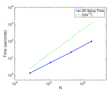
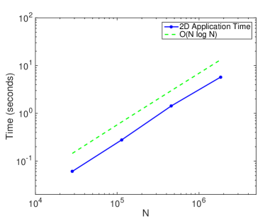
Figure 1: The $\log$-$\log$ plots of the scalings of the runtimes in 2D. The runtimes are taken as the averages of $T_{\text{setup}}$ and $T_{\text{apply}}$ of the three test cases. Left: Setup time scaling. Right: Application time scaling. The solid lines are the actual runtimes and the dashed lines are the theoretical scalings. We see that the application time scales as the theoretical cost, while the setup time scales far below, benefiting from MATLAB’s built-in parallelization.

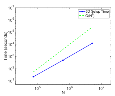
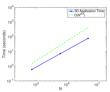
Figure 2: The $\log$-$\log$ plots of the scalings of the runtimes in 3D. The runtimes are taken as the averages of $T_{\text{setup}}$ and $T_{\text{apply}}$ of the three test cases. Left: Setup time scaling. Right: Application time scaling. The solid lines are the actual runtimes and the dashed lines are the theoretical scalings. The setup cost scales below the theoretical cost, which is credited to MATLAB’s built-in parallelization.

5 Conclusions and future work

This paper presents the sparsifying preconditioner for the time-harmonic Maxwell’s equations. The key idea is to transform the dense linear system into a sparse one by minimizing the non-local interactions. As shown by the numerical results, when combined with the standard GMRES solver, the preconditioner converges in only a few iterations, essentially independent of the problem size. The setup and application costs are almost the same as the ones for solving the sparse system arising from the PDE formulation.

There are several potential improvements that can be made. First, the problem considered in this paper only involves inhomogeneity for the electric permittivity $\varepsilon$. Indeed, the magnetic permeability $\mu$ can be inhomogeneous as well. The only difference is that, by taking the inhomogeneity of $\mu$ into account, one needs to deal with a larger integral system with both $E$ and $H$ involved. Nevertheless, the same idea applies and the integral system can be sparsified with a similar procedure. Second, instead of solving the sparsified system with the nested dissection method, the sweeping preconditioner [10, 11] could be applied to further reduce the computational cost. There are several previous works indicating the validity of this approach. For example, [19, 20] applied the sweeping preconditioner to the time-harmonic Maxwell’s equations. [15] combined the sweeping preconditioner with the sparsifying preconditioner and formed an efficient preconditioner that solves the Lippmann-Schwinger equation in quasi-linear time. By combining the two preconditioners alongside with a recursive approach similar to [14], we could hopefully reduce the cost of solving the integral form of the time-harmonic Maxwell’s equations to quasi-linear as well.

References

- [1] I. M. Babuška and S. A. Sauter. Is the Pollution Effect of the FEM Avoidable for the Helmholtz Equation Considering High Wave Numbers? SIAM Journal on Numerical Analysis, 34(6):2392–2423, 1997.
- [2] J.-P. Berenger. A perfectly matched layer for the absorption of electromagnetic waves. J. Comput. Phys., 114(2):185–200, 1994.
- [3] G. Beylkin, C. Kurcz, and L. Monzón. Fast convolution with the free space Helmholtz Green’s function. Journal of Computational Physics, 228(8):2770–2791, 2009.
- [4] N. J. Champagne II, J. G. Berryman, and H. M. Buettner. FDFD: A 3D finite-difference frequency-domain code for electromagnetic induction tomography. Journal of Computational Physics, 170(2):830–848, 2001.
- [5] W. C. Chew and W. H. Weedon. A 3D perfectly matched medium from modified Maxwell’s equations with stretched coordinates. Microw. Opt. Techn. Let., 7(13):599–604, 1994.
- [6] D. Colton and R. Kress. Inverse acoustic and electromagnetic scattering theory, volume 93. Springer Science & Business Media, 2012.
- [7] J. W. Cooley and J. W. Tukey. An algorithm for the machine calculation of complex Fourier series. Mathematics of computation, 19(90):297–301, 1965.
- [8] R. Duan and V. Rokhlin. High-order Quadratures for the Solution of Scattering Problems in Two Dimensions. J. Comput. Phys., 228(6):2152–2174, Apr. 2009.
- [9] I. S. Duff and J. K. Reid. The multifrontal solution of indefinite sparse symmetric linear equations. ACM Trans. Math. Software, 9(3):302–325, 1983.
- [10] B. Engquist and L. Ying. Sweeping preconditioner for the Helmholtz equation: hierarchical matrix representation. Comm. Pure Appl. Math., 64(5):697–735, 2011.
- [11] B. Engquist and L. Ying. Sweeping preconditioner for the Helmholtz equation: moving perfectly matched layers. Multiscale Model. Simul., 9(2):686–710, 2011.
- [12] A. George. Nested dissection of a regular finite element mesh. SIAM J. Numer. Anal., 10:345–363, 1973. Collection of articles dedicated to the memory of George E. Forsythe.
- [13] S. G. Johnson. Notes on Perfectly Matched Layers (PMLs). Lecture notes, Massachusetts Institute of Technology, Massachusetts, 2008.
- [14] F. Liu and L. Ying. Recursive sweeping preconditioner for the three-dimensional Helmholtz equation. SIAM Journal on Scientific Computing, 38(2):A814–A832, 2016.
- [15] F. Liu and L. Ying. Sparsify and Sweep: An Efficient Preconditioner for the Lippmann–Schwinger Equation. SIAM Journal on Scientific Computing, 40(2):B379–B404, 2018.
- [16] J. W. H. Liu. The multifrontal method for sparse matrix solution: theory and practice. SIAM Rev., 34(1):82–109, 1992.
- [17] C. Müller. Foundations of the mathematical theory of electromagnetic waves, volume 155. Springer Science & Business Media, 2013.
- [18] J.-C. Nédélec. Mixed finite elements in . Numerische Mathematik, 35(3):315–341, 1980.
- [19] P. Tsuji, B. Engquist, and L. Ying. A sweeping preconditioner for time-harmonic Maxwell’s equations with finite elements. Journal of Computational Physics, 231(9):3770–3783, 2012.
- [20] P. Tsuji and L. Ying. A sweeping preconditioner for Yee’s finite difference approximation of time-harmonic Maxwell’s equations. Frontiers of Mathematics in China, 7(2):347–363, 2012.
- [21] K. Yee. Numerical solution of initial boundary value problems involving Maxwell’s equations in isotropic media. IEEE Transactions on antennas and propagation, 14(3):302–307, 1966.
- [22] L. Ying. Sparsifying Preconditioner for Pseudospectral Approximations of Indefinite Systems on Periodic Structures. Multiscale Modeling & Simulation, 13(2):459–471, 2015.
- [23] L. Ying. Sparsifying Preconditioner for the Lippmann-Schwinger Equation. Multiscale Modeling & Simulation, 13(2):644–660, 2015.