A Lagrangian stochastic model of a volcanic eruption column

Abstract

We develop a Lagrangian stochastic model (LSM) of a volcanic plume in which the mean flow is provided by an integral plume model of the eruption column and fluctuations in the vertical velocity are modelled by a suitably constructed stochastic differential equation. The LSM is applied to the two eruptions considered by Costa et al. (2016) for the volcanic-plume intercomparison study. Vertical profiles of the mass concentration computed from the LSM are compared with equivalent results from a large-eddy simulation (LES) for the case of no ambient wind. The LSM captures the order of magnitude of the LES mass concentrations and some aspects of their profiles. In contrast with a standard integral plume model, i.e. without fluctuations, the mass concentration computed from the LSM decays (to zero) towards the top of the plume which is consistent with the LES plumes. In the lower part of the plume, we show that the presence of ash leads to a peak in the mass concentration at the level at which there is a transition from a negatively buoyant jet to a positively buoyant plume. The model can also account for the ambient wind and moisture.

1 Introduction

Volcanic plumes represent the most powerful naturally occuring buoyant sources of airborne contaminants. The spread of volcanic ash downwind of the eruption column presents a significant hazard to aviation which motivates the development of mathematical models that enable its prediction. Models of the eruption column play a role in quantifying a volcanic source for a long-range dispersion model. While simple one-dimensional integral models of volcanic plumes (see e.g. Woods, 1988, 1993; Glaze et al., 1997; Mastin, 2007; Devenish, 2013; Costa et al., 2016, and references therein) can provide the variation with height of bulk properties of the plume including the mass concentration, this latter quantity has the unfortunate property that it blows up at the top of the plume. The vertical profile of mass concentration produced by an integral model is then not suitable for initialising a long-range dispersion model. One purpose of this letter is to present a model that can provide a more realistic vertical profile of the mass concentration.

A second motivation for this study is the development of a model for the explicit treatment of volcanic plumes within a long-range dispersion model. Models of turbulent dispersion often take a Lagrangian form which provides a natural framework for modelling, for example, dispersion from a point source which is harder to model with an Eulerian approach. Typically, thousands of model particles are followed through a given flow field and statistics such as the mean concentration are calculated from the ensemble of particles. The resolved part of the flow field would, for realistic applications, normally be taken from a numerical weather prediction model while the unresolved part of the motion is modelled by means of random increments to the velocity of the particles. These models, which are known as Lagrangian stochastic models (LSMs), can be rigorously formulated (Thomson, 1987) and have been very successful at reproducing observations (e.g. Thomson & Wilson, 2012).

In most realistic dispersion models that are used for operational purposes, the Lagrangian particles move independently of each other through the flow field. There is then an inherent difficulty in modelling a coherent process such as a volcanic plume using single-particle LSMs: the motion of individual particles or fluid elements depends on the buoyancy of all the fluid elements. Moreover, there is nothing to constrain two neighbouring model particles to be moving upwards with similar velocities.

Several authors have attempted to model simple Boussinesq plumes using a Lagrangian approach (e.g. Luhar & Britter, 1992; Anfossi et al., 1993; Weil, 1994; Heinz & van Dop, 1999; Alessandrini et al., 2013; Marro et al., 2014). In particular we consider the approach developed by Webster and Thomson (2002) and Bisignano and Devenish (2015) in which the mean flow is calculated from an integral plume model and the fluctuations are calculated using a suitably formulated stochastic differential equation (sde). Here we extend this approach to the modelling of volcanic plumes.

In the next section we present the LSM which is formulated for a realistic atmosphere with non-uniform stability, ambient wind and moisture. In section 3 we consider numerical solutions of the LSM for various different cases: in particular we compare solutions of the LSM with an equivalent large-eddy simulation (LES) in the case of no ambient wind.

2 Lagrangian Stochastic Model

The model of Devenish (2013) is used to provide the mean flow. The governing equations take the form

$$\frac{dQ_{m}}{dt} = E\overline{v}_{p}$$ (1)

$$\frac{dM_{z}}{dt} = (\rho_{a}-\rho_{p})g\pi b^{2}\overline{v}_{p}$$ (2)

$$\frac{dM_{i}}{dt} = -Q_{m}\frac{dU_{i}}{dt}\qquad i=x,y$$ (3)

$$\frac{dH}{dt} = \left((1-q_{va})c_{pd}+q_{va}c_{pv}\right)T_{a}E\overline{v}_{p}-g\rho_{a}\pi b^{2}\overline{v}_{p}\overline{w}_{p}$$ (4)

$$+\left[L_{v0}-273(c_{pv}-c_{pl})\right]\frac{dQ_{l}}{dt}$$

$$\frac{dQ_{t}}{dt} = Eq_{va}\overline{v}_{p}$$ (5)

where, at time $t$, $Q_{m}=\rho_{p}\pi b^{2}\overline{v}_{p}$ is the mass flux; $Q_{t}=n_{t}Q_{m}$ is the total moisture flux (water vapour and liquid water; the model contains no ice); $Q_{l}=n_{l}Q_{m}$ is the flux of liquid water; $M_{i}=(u_{pi}-U_{i})Q_{m}$ ($i=x,y$) are the horizontal components of the momentum flux; $M_{z}=\overline{w}_{p}Q_{m}$ is the vertical component of the momentum flux; and $H=c_{pp}T_{p}Q_{m}$ is the enthalpy flux. In equations (1)–(5) and the expressions for the fluxes $\overline{v}_{p}=\sqrt{u_{px}^{2}+u_{py}^{2}+\overline{w}_{p}^{2}}$ is the total velocity in which $u_{pi}$ ($i=x,y$) are the horizontal components of the plume velocity and $\overline{w}_{p}$ is the vertical component of the plume velocity; $n$ is a mass fraction and the subscripts $l$, $v$ and $t$ refer to liquid water, water vapour and the total moisture content respectively and we have $n_{t}=n_{v}+n_{l}$; $c_{pp}$ is the bulk specific heat capacity of the plume (to be defined below); $b$ is the plume radius; $g$ is the acceleration due to gravity; $q_{v}$ is the humidity; $\rho$ is the density and $T$ is the plume temperature; a subscript $a$ refers to ambient whereas a subscript $p$ refers to plume. The horizontal coordinates are $x$ and $y$ and $z$ indicates the vertical coordinate. In equation (3) the components of the ambient wind speed are indicated by $U_{i}$ ($i=x,y$). In equation (4) $c_{pd}$, $c_{pv}$ and $c_{pl}$ are the specific heat capacities at constant pressure of the dry air, water vapour and liquid water respectively; $L_{v0}$ is the latent heat of vaporisation at 0${}^{\mbox{\footnotesize{o}}}$ C.

The entrainment, $E$, is determined following Devenish (2013) as are phase changes between water vapour and liquid water. Similarly, the plume density, bulk gas constant and bulk specific heat capacity are also calculated following Devenish (2013). The evolution of the mass fraction of gas is determined assuming that there is no fall out of material (both ash and liquid water) during the evolution of the plume (see Devenish (2013) for more details).

In the construction of the model, it is useful to re-write equation (2) as an equation for the vertical velocity:

$$\frac{d\overline{w}_{p}}{dt}=\frac{g(\rho_{a}-\rho_{p})}{\rho_{p}}-\frac{\overline{v}_{p}\overline{w}_{p}E}{Q_{m}}.$$ (6)

Equation (6) makes clear that the evolution of $\overline{w}_{p}$ depends on the local buoyancy of the plume and that entrainment produces a deceleration of the plume. The sde. for the fluctuating vertical velocity, $w_{p}^{\prime}$, is constructed from an analogous equation to equation (6) coupled with an LSM for $w_{p}^{\prime}$ appropriate for inhomogeneous turbulence. Since we assume there are no fluctuations in $\rho$ (either in the plume or in the environment), the sde for $w_{p}^{\prime}$ is given by

$$dw_{p}^{\prime}=-\frac{\overline{v}_{p}w_{p}^{\prime}E}{Q_{m}}dt-\frac{w_{p}^{\prime}}{T_{L}}dt+\frac{1}{2}\left(\frac{1}{w_{p}}+\frac{w_{p}^{\prime}}{\sigma_{w}^{2}}\right)d\sigma_{w}^{2}+\frac{\sigma_{w}^{2}}{w_{p}\rho_{p}}\,d\rho_{p}+\sqrt{C_{0}\varepsilon}\,dW$$ (7)

where $w_{p}=\overline{w}_{p}+w_{p}^{\prime}$, $T_{L}$ is the time scale on which $w_{p}^{\prime}$ changes, $\sigma_{w}^{2}$ is the vertical-velocity variance, $\varepsilon$ is the mean kinetic energy dissipation rate, $dW$ is the increment of a Wiener process and $C_{0}$ is the constant of proportionality in the second-order Lagrangian velocity structure function which typically has a value in the range $5-7$ for homogeneous isotropic turbulence (e.g. Yeung, 2002); we choose $C_{0}=6$. The first term on the right-hand side (rhs) of equation (7) represents entrainment-related turbulence and is motivated by the form of equation (6) and consistency with Bisignano and Devenish (2015). The last four terms on the rhs of equation (7) are those of Thomson (1987)’s LSM for inhomogeneous turbulence (as would be the case for a one-point Gaussian joint velocity-density distribution). Note that the penultimate term on the rhs is often neglected (Stohl & Thomson, 1999) but, as will be shown below, can be significant.

It remains to specify the forms of $\sigma_{w}^{2}$, $T_{L}$ and $\varepsilon$ which are all functions of $z$. We expect $\sigma_{w}$ to scale with $\overline{w}$ and $T_{L}$ to be related to the appropriate mean quantities in the problem. Hence, following Bisignano and Devenish (2015), we choose $\sigma_{w}=\alpha|\overline{w}_{p}|$, and $T_{L}=b/|\overline{w}_{p}|$. At the vent, $T_{L}$ is defined by the source radius and the exit velocity which is consistent with the eddy decorrelation time scale identified by Cerminara et al. (2016). Since

$$T_{L}=\frac{2\sigma_{w}^{2}}{C_{0}\varepsilon},$$

(e.g. Pope, 2000, p.486) it follows that

$$\varepsilon=\frac{2\alpha^{2}\overline{w}_{p}^{2}|\overline{w}_{p}|}{C_{0}b}.$$

3 Numerical Solution of the LSM

The LSM presented in the previous section i.e. equations (1), (3) – (5), (6) and (7) are solved simultaneously using an Euler-Maruyama method. The fluctuating velocity component is initially drawn from a Gaussian distribution with mean zero and variance $\sigma_{w}^{2}$. The results are computed following 100,000 independently moving particles. Integration is terminated for each particle when $\overline{w}_{p}$ becomes zero. The mass concentration per unit length, $C$, is calculated according to

$$C(z)=\frac{Q_{m0}}{\Delta z\,N_{p}}\sum_{N_{t}}(\#\,\mbox{particles in each box})\,\Delta t$$

where $\Delta z$ is the depth of each box, $N_{p}$ is the number of particles, $N_{t}$ is the number of time steps and $\Delta t$ is the time step (or residence time).

Results are presented for two eruptions: the weak and strong eruptions considered by Costa et al. (2016) with and without the ambient wind. The weak eruption is the 26 January 2011 Shinmoe-dake eruption in Japan that produced a plume that reached about 8 km above sea level (Hashimoto et al., 2012; Kozono et al., 2013; Suzuki & Koyaguchi, 2013). The strong eruption is based on the climactic phase of the Pinatubo eruption, Philippines, on 15 June 1991, during which the eruption column reached about 39 km above sea level (Koyaguchi & Tokuno, 1993; Holasek et al., 1996; Costa et al., 2013). The source mass fluxes for each case are 1.5 Gg s^-1 and 1.5 Tg s^-1 respectively. The same initial conditions and profiles of the ambient quantities as used by Costa et al. (2016) are also used here.

The results of the LSM are compared with corresponding results from a recent LES (Cerminara et al., 2016) for the case of no ambient wind. The LES plume region is defined as the subdomain where the mass fraction of a tracer is larger than 0.1% of its initial value. The maximum rise height of the LES plumes is determined from the mass flux: it is the level at which the mass flux falls below 1% of its value at the vent (see Cerminara et al., 2016, for more details). The level of neutral buoyancy, $z_{eq}$, is 9.3 km above mean sea level (msl) for the weak eruption and 20.3 km (above msl) for the strong eruption (Cerminara et al., 2016). The jet length scale, $L_{M}$, is the characteristic height at which the initial momentum-dominated jet becomes a buoyancy dominated plume. For a volcanic plume, $L_{M}$ is defined as (Cerminara, 2016, Section 3.6)

$$L_{M}=\frac{L_{0}}{(2\alpha\mbox{Ri})^{1/2}}$$

where

$$L_{0}=\frac{Q_{m}}{\sqrt{\pi\rho_{a}M_{z}}}=b\sqrt{\frac{\rho_{p}}{\rho_{a}}}\sqrt{\frac{\overline{v}_{p}}{\overline{w}_{p}}}$$

$$\mbox{Ri}=\frac{\phi\,gQ_{m}^{3}}{\sqrt{\pi\rho_{a}M_{z}^{5}}}=\frac{\phi gb}{\overline{w}_{p}^{2}}\sqrt{\frac{\rho_{p}}{\rho_{a}}}\sqrt{\frac{\overline{v}_{p}}{\overline{w}_{p}}}$$

and $\phi=h_{p}/h_{a}-1$ where $h_{p}$ and $h_{a}$ are the specific enthalpies of the plume and the environment respectively. The plume properties and those of the environment are evaluated at the vent level. In the Boussinesq limit $L_{0}$ reduces to the vent radius for a vertically rising plume; in practice $\overline{v}_{p}\approx\overline{w}_{p}$ for a volcanic plume at the vent. In the same limit, $L_{M}$ reduces to the jet length scale defined by Morton (1959). For forced plumes such as volcanic plumes, $L_{0}\ll L_{M}$. For the weak eruption $L_{M}\approx 0.35$ km and for the strong eruption $L_{M}\approx 4$ km. At the vent level the plume is a mixture of three components: water, coarse particles and fine particles. For the weak eruption, the mass fractions are 3 wt.%, 48.5 wt% and 48.5 wt.% respectively; coarse particles have a diameter of 1 mm and fine particles a diameter of 62.5 $\mu$m. For the strong eruption the mass fractions are 5 wt.%, 47.5 wt% and 47.5 wt.% respectively; coarse particles have a diameter of 500 $\mu$m and fine particles a diameter of 16 $\mu$m. The LES results to be presented below are for the upwardly rising core of the plume.

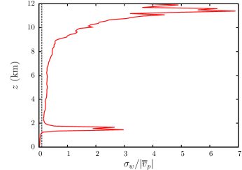
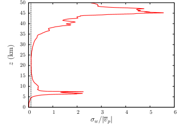
Figure 1: The variation with height of $\sigma_{w}/|\overline{v}_{p}|$ (red) for the LES plume for the (a) weak and (b) strong eruptions. In both figures the dashed black line represents the value $\sigma_{w}/|\overline{v}_{p}|=0.1$.

Figure 1 shows the variation with height of the ratio $\sigma_{w}/|\overline{v}_{p}|$ along the centreline of the LES plumes. (Note that $\overline{v}_{p}\approx\overline{w}_{p}$ over most of the depth of the plume except at heights of order $L_{M}$ and at the plume top where $\overline{w}_{p}$ becomes zero.) It shows that the assumption that $\sigma_{w}=\alpha\overline{w}_{p}$ where $\alpha=0.1$ is reasonable in the positively buoyant part of the plume i.e. the region between $L_{M}$ and $z_{eq}$.

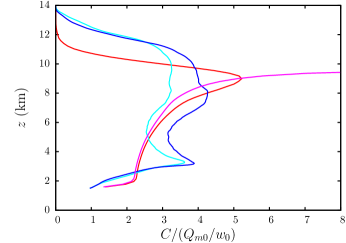
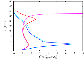
Figure 2: The variation with height of the normalised concentration for the (a) weak and (b) strong eruptions. In each figure the red line represents the LSM, the magenta line the LSM with no turbulence, the cyan line the LES with the coarse mass fraction and the blue line the LES with the fine mass fraction. In the normalisation of the concentration, the subscript ‘0’ represents the initial value at the vent.

The vertical profile of the mass concentration in the LSM is shown in Figure 2 for the case of no ambient wind both with and without turbulence. The latter case amounts to solving the plume equations alone i.e. equations (1) – (5) such that the concentration is given by $\pi b^{2}\rho_{s}$. Figure 2 clearly shows that turbulent fluctuations have very little effect on the concentration profile in the lower part of the plume but that without turbulent fluctuations the mass concentration increases very rapidly towards the top of the plume. This behaviour is explained by the fact that as $\overline{w}_{p}\rightarrow 0$ at the top of the plume, $b\rightarrow\infty$ (since $Q_{m}$ grows monotonically with height). In the case with turbulent fluctuations, particles have different values of $z$ when $\overline{w}_{p}=0$ and this gives rise to the smooth peak which decays to zero at the top of the plume.

Figure 2 also shows the vertical profiles of the mass concentration for the LES plume (i.e. $\int_{S(z)}\rho_{p}(x,y,z)\,dx\,dy$ where $S(z)$ is a horizontal slice at height $z$ of the LES plume region with positive vertical velocity). It can be seen that the maximum rise height of the LSM plume is broadly consistent with that of the LES plume. The LSM plume is better at capturing the order of magnitude of the concentration and the vertical structure of the LES plume for the weak eruption than the strong eruption. This is also evident in the total mass within the plume (i.e. $\int C(z)\,dz$) shown in Table 1 for the weak and strong eruptions. The vertical profile of the LES plume for the weak eruption shows a distinct lower peak and a broader higher peak. The profile for the strong eruption is dominated by the lower peak. The equivalent LSM plumes show pronounced upper peaks but only incipient lower peaks especially for the weak eruption. For both the weak and strong eruptions, the height of the upper peak in the LSM plume is consistent with the level of maximum radial spread found by Suzuki et al. (2016). The presence of the solid phase in the LES plumes can lead to partial column collapse, particle settling and re-circulation especially at $z\sim L_{M}$. This is particularly prevalent in the strong eruption and leads to the formation of the significant lower peak in the concentration profile as shown in Figure 2b. However, since these processes are absent in the LSM, it does not explain why the LSM plume also exhibits a lower peak.

Case	LSM	LES
		Coarse	Fine	Total
Weak	317 Gg	192 Gg	164 Gg	356 Gg
Strong	308 Tg	195 Tg	210 Tg	405 Tg

Table 1: The total mass in the LSM and LES plumes.

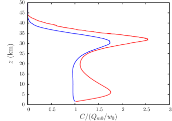
Figure 3: The normalised concentration for the LSM plume: (a) weak and (b) strong eruptions. In each figure the red line represents the default case i.e. an ash rich plume (as shown in Figure 2) and the blue line represents the case of a gas-only plume.

Figure 3 shows the LSM plumes with and without ash for both the weak and strong eruptions. In the absence of ash, the concentration does not exhibit a lower peak for either the weak or strong eruptions; this is particularly noteworthy for the strong eruption. The height of the lower peak occurs, to a good approximation, at a distance $L_{M}$ above the vent, the height associated with buoyancy reversal i.e. a transition from negative to positive buoyancy. In the LES plume this is the height at which partial column collapse tends to occur since material above this height is more likely to be carried aloft by the positive buoyancy. In the absence of ash, the plume is dominated by buoyancy from the vent upwards and so no transition occurs.

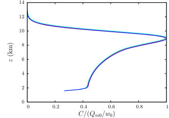
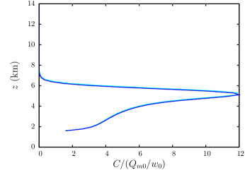
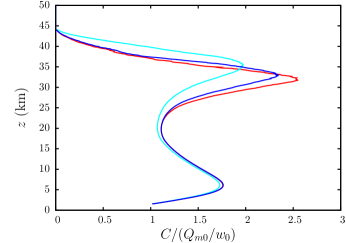
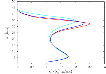
Figure 4: The normalised concentration for the weak (top row) and strong (bottom row) eruptions. The left-hand column is the case without the ambient wind and the right-hand column is the case with the ambient wind. In each figure the red line is the default case (as shown in Figure 2), the blue line the LSM without moisture and the cyan line the LSM with no density correction.

The LSM can be used to assess the importance of a number of different physical processes. In Figure 4 we show the effect of the ambient wind, moisture and the acceleration due to the change in density with height (as represented by the penultimate term on the rhs of equation (7)). For all these cases, no equivalent LES data is available. It is immediately clear that the ambient wind has a significant effect on the rise height of the weak eruption with no appreciable effect on the qualitative morphology of the concentration profile. It is also clear that neither moisture nor the density correction have any noticeable impact on this case. For the strong eruption, it is clear that the ambient wind has no effect but that the moisture has a small effect on the vertical structure of the plume; the same can be said for the density correction.

4 Conclusions

We have presented an LSM of a volcanic plume in which an integral volcanic-plume model provides the mean flow and a suitably constructed sde gives the fluctuating vertical velocity. We compared the mass concentration computed from the LSM with data from a corresponding LES for the two eruptions considered in the volcanic-plume intercomparison study of Costa et al. (2016). The LSM captures the order of magnitude of the mass concentration and aspects of its vertical profile. In qualitative agreement with the LES results, the LSM mass concentration decays to zero at the top of the plume. In contrast, the mass concentration computed from a standard integral plume model, i.e. without fluctuations, blows up at the top of the plume. As with the integral plume models considered in Costa et al. (2016) the LSM compares relatively well with the weak eruption but not so well with the strong eruption. The reasons for this are complex but are likely to include a relatively small aspect ratio and a relatively small ratio of $z_{eq}$ to $L_{M}$ compared with the weak eruption. We showed that the presence of ash alone is sufficient to produce a peak in the mass concentration at $z\sim L_{M}$, the height at which there is a transition from a negatively buoyant jet to a positively buoyant plume. Although for the LES plume the magnitude of this peak is likely to be determined by the complex flow features in the LES, their absence in the LSM and the standard integral plume model suggests that $L_{M}$ plays an important role in the LES plume as well.

The LSM developed here is designed to be used with realistic meteorological profiles including the ambient wind and moisture. An analysis of the effect of ambient conditions on the two eruption columns showed that, as expected, the ambient wind affected the weak eruption but not the strong eruption. In contrast, ambient moisture had a small effect on the strong eruption but almost no effect on the weak eruption. The LSM can be used to provide a vertical distribution of material for use in an operational dispersion model where the eruption column is often modelled as a uniform passive line source. Furthermore, it could be incorporated into a Lagrangian dispersion model to provide a dynamic source.

The LES data can be accessed at the repository:
vmsg.pi.ingv.it/uploads/files/publications/LES_data.zip

References

- Alessandrini et al. (2013) Alessandrini, S., Ferrero, E., & Anfossi, D. (2013). A new Lagrangian method for modelling the buoyant plume rise. Atmospheric Environment 77, 239-249.
- Anfossi et al. (1993) Anfossi, D., Ferrero, E., Brusasca, G., Marzorati, A., & Tinarelli, G. (1993). A simple way of computing buoyant plume rise in Lagrangian stochastic dispersion model. Atmospheric Environment 27A, 1443-1451.
- Bisignano and Devenish (2015) Bisignano, A., & Devenish, B. J. (2015). A model for temperature fluctuations in a buoyant plume. Boundary-Layer Meteorology 157, 157-172.
- Cerminara (2016) Cerminara, M. (2016). Modeling dispersed gas-particle turbulence in volcanic ash plumes (Doctoral dissertation). Pisa, Italy: Scuola Normale Superiore.
- Cerminara et al. (2016) Cerminara, M., Esposti Ongaro, T., & Neri, A. (2016). Large Eddy Simulation of gas-particle kinematic decoupling and turbulent entrainment in volcanic plumes. Journal of Volcanology and Geothermal Research 326, 143-171.
- Costa et al. (2013) Costa, A., Folch, A., Macedonio, G. (2013). Density-driven transport in the umbrella region of volcanic clouds: implications for tephra dispersion models. Geophysical Research Letters 40, 4823-4827.
- Costa et al. (2016) Costa, A., Suzuki, Y. J., Cerminara, M., Devenish, B. J., Esposti Ongaro, T., Herzog, M., …Bonadonna, C. (2016). Results of the eruptive column model inter-comparison study. Journal of Volcanology and Geothermal Research 326, 2-25.
- Devenish (2013) Devenish, B. J. (2013). Using simple plume models to refine the source mass flux of volcanic eruptions according to atmospheric conditions. Journal of Volcanology and Geothermal Research 256, 118-127.
- Glaze et al. (1997) Glaze, L. S., Baloga, S. M., & Wilson. L. (1997). Transport of atmospheric water vapor by volcanic eruption columns. Journal of Geophysical Research 102, 6099-6108.
- Hashimoto et al. (2012) Hashimoto, A., Shimbori, T., & Fukui, K. (2012). Tephra fall simulation for the eruptions at Mt. Shinmoe-dake during 26-27 January 2011 with JMANHM. Scientific online letters on the atmosphere (SOLA) 8, 37-40.
- Heinz & van Dop (1999) Heinz, S., van Dop, H. (1999). Buoyant plume rise described by a Lagrangian turbulence model. Atmospheric Environment 33, 2031-2043.
- Holasek et al. (1996) Holasek, R., Self, S., & Woods, A. (1996). Satellite observations and interpretation of the 1991 Mount Pinatubo eruption plumes. Journal of Geophysical Research 101, 27635-27655.
- Koyaguchi & Tokuno (1993) Koyaguchi, T., & Tokuno, M., (1993). Origin of the giant eruption cloud of Pinatubo, June 15, 1991. Journal of Volcanology and Geothermal Research 55, 85-96.
- Kozono et al. (2013) Kozono, T., Ueda, H., Ozawa, T., Koyaguchi, T., Fujita, E., Tomiya, A., & Suzuki, Y. J. (2013). Magma discharge variations during the 2011 eruptions of Shinmoe-dake volcano, Japan, revealed by geodetic and satellite observations. Bulletin of Volcanology 75, 695.
- Luhar & Britter (1992) Luhar, A.K., Britter, R.E. (1992). Random walk modelling of buoyant-plume dispersion in the convective boundary layer. Atmospheric Environment 26A, 1283-1298.
- Marro et al. (2014) Marro, M., Salizzoni, P., Cierco, F. X., Korsakissok, I., Danzi, E., & Soulhac, L. (2014). Plume rise and spread in buoyant releases from elevated sources in the lower atmosphere. Environmental Fluid Mechanics 14, 201-219.
- Mastin (2007) Mastin, L. G. (2007). A user-friendly one-dimensional model for wet volcanic plumes. Geochemistry, Geophysics, Geosystems 8, Q03014.
- Morton (1959) Morton, B. R. (1959). Forced plumes. Journal of Fluid Mechanics 5, 151-163.
- Pope (2000) Pope, S. B. (2000). Turbulent flows. Cambridge: Cambridge University Press.
- Ricou & Spalding (1961) Ricou, F. P., & Spalding, D. B. (1961). Measurements of entrainment by axisymmetrical turbulent jets. Journal of Fluid Mechanics, 8, 21-32.
- Stohl & Thomson (1999) Stohl, A., & Thomson, D. J. (1999). A density correction for Lagrangian particle dispersion models. Boundary-Layer Meteorology 90, 155-167.
- Suzuki & Koyaguchi (2013) Suzuki, Y. J., & Koyaguchi, T. (2013). 3D numerical simulation of volcanic eruption clouds during the 2011 Shinmoe-dake eruptions. Earth Planets Space 65, 581-589.
- Suzuki et al. (2016) Suzuki, Y. J., Costa, A., Cerminara, M., Esposti Ongaro, T., Herzog, M., Van Eaton, A. R., & Denby, L. C. (2016). Inter-comparison of three-dimensional models of volcanic plumes. Journal of Volcanology and Geothermal Research 326, 26-42.
- Thomson (1987) Thomson, D. J. (1987). Criteria for the selection of stochastic models of particle trajectories in turbulent flows. Journal of Fluid Mechanics 180, 529-556.
- Thomson & Wilson (2012) Thomson, D. J., & Wilson, J. D. (2012). History of Lagrangian stochastic models for turbulent dispersion. In J. Lin, D. Brunner, C. Gerbig, A. Stohl, A. Luhar, P. Webley (Eds.), Lagrangian Modelling of the Atmosphere, Geophysical Monograph Series (Vol. 200, 19-36). Washington, DC: American Geophysical Union.
- Webster and Thomson (2002) Webster, H. N., & Thomson, D. J. (2002). Validation of a Lagrangian model plume rise scheme using the Kincaid data set. Atmospheric Environment 36, 5031-5042.
- Weil (1994) Weil, J. C. (1994). A hybrid Lagrangian dispersion model for elevated sources in the convective boundary layer. Atmospheric Environment 28, 3433-3448.
- Woods (1988) Woods, A. W. (1988). The fluid dynamics and thermodynamics of eruption columns. Bulletin of Volcanology 50, 169-193.
- Woods (1993) Woods, A.W. (1993). Moist convection and the injection of volcanic ash into the atmosphere. Journal of Geophysical Research 98, 17627-17636.
- Yeung (2002) Yeung, P. K. (2002). Lagrangian investigations of turbulence. Annual Review of Fluid Mechanics 34, 115-142.