A meshfree particle method for a vision-based macroscopic pedestrian model

Abstract

In this paper we present numerical simulations of a macroscopic vision-based model [2] derived from microscopic situation rules described in [3]. This model describes an approach to collision avoidance between pedestrians by taking decisions of turning or slowing down based on basic interaction rules, where the dangerousness level of an interaction with another pedestrian is measured in terms of the derivative of the bearing angle and of the time-to-interaction. A meshfree particle method is used to solve the equations of the model. Several numerical cases are considered to compare this model with models established in the field, for example, social force model coupled to an Eikonal equation [4]. Particular emphasis is put on the comparison of evacuation and computation times.

Keywords: Interacting particle system; Pedestrian dynamics; Collision avoidance; Bearing angle; Time-to-interaction; Macroscopic limits; Particle method; Social force model.

1 Introduction

To achieve a better comprehension of crowd behavior and increase the reliability of predictions, numerical modeling and simulation of human crowd motion have become a major subject of research with a wide field of applications. These include planning the architecture of buildings, supporting transport planners or managers to design timetables, improving efficiency and safety in public places such as airport terminals, train stations, theaters and shopping malls.

Several models of pedestrian behavior have been proposed on different levels of description in recent years. The Individual-Based Models (or IBM) such as models based on heuristic rules [5], Newton type equations [6, 7, 8, 9], traffic following models [10], cellular-automata [11, 12], agent-based models [13, 14], optimal control theory models [15], mechanical models [16, 17] and vision-based models [3, 18, 19, 20, 21, 22, 23] have been developed. Macroscopic pedestrian flow model involving equation for density and mean velocity of the flow are derived in Refs. [2, 4, 24, 25, 26, 27, 28].

Pedestrians can estimate the positions and velocities of moving obstacles such as other pedestrians with fairly good accuracy, compare [29] and are able to process this information in order to determine the dangerousness level of an encounter [30]. With these considerations, the heuristic-based model of [31] proposes that pedestrians follow two phases: a perception phase and a decision-making phase.

In the perception phase, pedestrians make an assessment of the dangerousness of an encounter with the other pedestrians. In the decision-making phase, they take decisions of turning or slowing down based on this assessment. To make this assessment, each pedestrian senses the indicators of the dangerousness of the collision such as the derivative of the Bearing Angle (DBA), the Time-To-Interaction (TTI) and the minimal distance (MD) with each of his interaction partners. The Bearing angle is the angle between the walking direction and the line connecting the two interaction partners and its time derivative provides a sensor of the likeliness of a collision, a constant Bearing angle in time being associated with a risk of future collision. The TTI is the time needed by the subject to reach the interaction point from his current position. The MD is the distance where the distance between the collision subjects is minimal. Finally, the risk of future collisions is determined by combining these indicators DBA, TTI and MD. For detailed explanations and geometrical interpretations we refer [2].

Using these considerations, a macroscopic model has been derived in [2] from the vision-based Individual-Based Models (IBM) of [3]. Moreover, there, a procedure has been presented to approximate the macroscopic mean-field equations with a local approximation. These models will be investigated numerically in the present paper.

One main objective of the present paper is to develop a numerical scheme to simulate the vision-based pedestrian model on a macroscopic scale and to compare it to other models established in the field, for example, classical social force models [6, 4]. We use, as in Ref. [24], a particle method which is based on a Lagrangian formulation of these equations, where particles are used as moving grid points. Preliminary numerical comparisons of the macroscopic models are presented. Moreover, we note that the method presented here is easily extended to more complicated “real” life situations.

The reminder of the paper is organized as follows. Section 2 contains the macroscopic vision-based model for pedestrian flow from [2]. The local approximation of the macroscopic model is presented in section 3. Particle method used in the simulations is described in section 4. Section 5 contains the numerical results. We consider a bidirectional evacuation problem. A comparison between the solutions of the macroscopic equations from the vision-based model and social force model is presented together with a comparison of the associated evacuation as well as computational times. Finally, section 6 concludes the work.

2 Vision-based macroscopic pedestrian flow model from [2]

For completeness of the presentation we review the macroscopic vision-based model for pedestrian flow, see Refs.[2, 3]. For further details we refer to these papers. There, denoting the density of pedestrians by $\rho(x,\xi,t)$ and by $U(x,\xi,t)$ the mean velocity at position $x$ with target point $\xi$ at time $t$, the model is given by the following mass and momentum balance equations

$$\partial_{t}\rho+\nabla_{x}\cdot(c\rho U) =0,$$ (1)

$$\partial_{t}U+cU\cdot\nabla_{x}U =\omega_{\rho\delta_{U}}(x,U(x,\xi,t),\xi,t)U^{\perp}(x,\xi,t),$$ (2)

where $c$ is the constant speed of the pedestrians and $\omega_{\rho\delta_{U}}(x,U(x,\xi,t),\xi,t)$ is the angular velocity, defined in the following way. First one has to define the indicators of the dangerousness of the collision measured between a particle located at position $x\in\mathbb{R}^{2}$ with velocity direction $u\in\mathbb{S}^{1}$ to the relative target $\xi\in\mathbb{R}^{2}$ and its collision particle located at position $y\in\mathbb{R}^{2}$ with velocity direction $v\in\mathbb{S}^{1}$ to the relative target $\eta\in\mathbb{R}^{2}$. They are respectively denoted by $\tilde{\dot{\alpha}}(x,u,y,v)$, $\tilde{\tau}(x,u,y,v)$, $\tilde{D}(x,u,y,v)$ and $\tilde{\dot{\alpha}}_{g}(x,u,\xi)$ and defined as

$$\tilde{\dot{\alpha}}(x,\xi,y,\eta,t) =c\dfrac{(y-x)\times(U(y,\eta,t)-U(x,\xi,t))}{\arrowvert y-x\arrowvert^{2}},$$ (3)

$$\tilde{\tau}(x,\xi,y,\eta,t) =-\frac{1}{c}\dfrac{(y-x)\cdot(U(y,\eta,t)-U(x,\xi,t))}{\arrowvert U(y,\eta,t)-U(x,\xi,t)\arrowvert^{2}},$$ (4)

$$\tilde{D}(x,\xi,y,\eta,t) =\left(\arrowvert y-x\arrowvert^{2}-\left((y-x)\cdot\dfrac{U(y,\eta,t)-U(x,\xi,t)}{\arrowvert U(y,\eta,t)-U(x,\xi,t)\arrowvert}\right)^{2}\right)^{1/2},$$ (5)

$$\tilde{\dot{\alpha}}_{g}(x,u,\xi) =-c\dfrac{(\xi-x)\times U(x,\xi,t)}{\arrowvert\xi-x\arrowvert^{2}}.$$ (6)

Moreover, one defines

$$\tilde{S}_{\pm}(x,\xi,t)= \{(y,\eta)\in\mathbb{R}^{2}\times\mathbb{R}^{2}|\pm\tilde{\dot{\alpha}}(x,\xi,y,\eta,t)>0,\tilde{\tau}(x,\xi,y,\eta,t)>0,$$ (7)

$$\hskip 25.60747pt\tilde{D}^{2}(x,\xi,y,\eta,t)<R^{2},|\tilde{\dot{\alpha}}(x,\xi,y,\eta,t)|<\sigma(|\tilde{\tau}(x,\xi,y,\eta,t)|)\}$$

and

$$\tilde{\Phi}_{\pm} (x,\xi,t)$$ (8)

$$=\dfrac{\int_{(y,\eta)\in\tilde{S}_{\pm}(x,\xi,t)}\Phi(|\tilde{\dot{\alpha}}(x,\xi,y,\eta,t)|,|\tilde{\tau}(x,\xi,y,\eta,t)|)\rho(y,\eta,t)dyd\eta}{\int_{(y,\eta)\in\tilde{S}_{\pm}(x,\xi,t)}\rho(y,\eta,t)dyd\eta},$$

where the function $\Phi$ is given by

$$\Phi(|\tilde{\dot{\alpha}}(x,\xi,y,\eta,t)|, |\tilde{\tau}(x,\xi,y,\eta,t)|)$$

$$=\Phi_{0}\max\{\sigma(|\tilde{\tau}(x,\xi,y,\eta,t)|)-|\tilde{\dot{\alpha}}(x,\xi,y,\eta,t)|,0\}$$ (9)

and

$$\sigma(|\tilde{\tau}(x,\xi,y,\eta,t)|)=a+\dfrac{b}{(|\tilde{\tau}(x,\xi,y,\eta,t)|+\tau_{0})^{c}},$$ (10)

where $\tau_{0},a,b$ are positive constants and $\Phi_{0}$ is the positive proportionality constant.

Then $\omega_{\rho\delta_{U}}(x,U(x,\xi,t),\xi,t)$ is defined in the following:

1. If the current deviation to the goal is small, this means that $|\tilde{\dot{\alpha}}_{g}|$ is smaller than the reaction induced by collision avoidance, i.e.

   $$-\tilde{\Phi}_{-}(x,\xi,t)\leq\tilde{\dot{\alpha}}_{g}(x,\xi,t)\leq\tilde{\Phi}_{+}(x,\xi,t).$$ (11)

   Then

   $$\omega_{\rho\delta_{U}}(x,U(x,\xi,t),\xi,t)=$$ (12)

   $$-\tilde{\Phi}_{+}(x,\xi,t)H(|\tilde{\Phi}_{-}(x,\xi,t)-|\tilde{\dot{\alpha}}_{g}(x,\xi,t)||-|\tilde{\Phi}_{+}(x,\xi,t)-|\tilde{\dot{\alpha}}_{g}(x,\xi,t)||)$$

   $$+\tilde{\Phi}_{-}(x,\xi,t)H(|\tilde{\Phi}_{+}(x,\xi,t)-|\tilde{\dot{\alpha}}_{g}(x,\xi,t)||-|\tilde{\Phi}_{-}(x,\xi,t)-|\tilde{\dot{\alpha}}_{g}(x,\xi,t)||),$$

   where H is the Heaviside function. This formula states that the pedestrian determines the worst case in each direction (expression of $\tilde{\Phi}_{+}$ and $\tilde{\Phi}_{-}$) and then chooses the turning direction as the one which produces the smallest deviation to the goal.

2. If the deviation to the goal is large, i.e.

   $$\tilde{\dot{\alpha}}_{g}(x,\xi,t)<-\tilde{\Phi}_{-}(x,\xi,t)\quad\text{or}\quad\tilde{\dot{\alpha}}_{g}(x,\xi,t)>\tilde{\Phi}_{+}(x,\xi,t).$$ (13)

   Then

   $$\omega_{\rho\delta_{U}}(x,U(x,\xi,t),\xi,t)=\tilde{\dot{\alpha}}_{g}(x,\xi,t).$$ (14)

   In this case, the deviation to the goal is larger than the reaction to collisions and the decision is to restore a direction of motion more compatible to the goal.

The intensity of the force is non-local in space as the pedestrian anticipates the behavior of neighboring pedestrians to take a decision. In the next section the spatially local approximation is discussed .

3 Local approximations to the macroscopic model

In this section we state the spatially local approximation to the macroscopic model using the procedure explained in [2] for the local approximation to the mean-field kinetic model. One assumes that there exists a small dimensionless quantity $\lambda\ll 1$ such that

$$R=\lambda\hat{R},\hskip 5.69054pt\Phi_{0}=\lambda\hat{\Phi_{0}},\hskip 5.69054pta=\frac{1}{\lambda}\hat{a},\hskip 5.69054pt\tau_{0}=\lambda\hat{\tau}_{0},\hskip 5.69054ptb=\lambda^{c-1}\hat{b},\hskip 5.69054pt\sigma=\frac{1}{\lambda}\hat{\sigma},$$ (15)

where all ‘hat’ quantities are assumed to be $\mathcal{O}(1)$. One introduces a change of variables $y=x+\lambda\zeta$, with $\zeta\in\mathbb{R}^{2}$ in all expressions involving $y$. This yields the expression for equations (3) - (5) as

$$\tilde{\dot{\alpha}}(x,\xi,y,\eta,t) =\frac{1}{\lambda}\hat{\dot{\alpha}}(\zeta,U(y,\eta,t)-U(x,\xi,t)),\hskip 5.69054pt\mbox{where}$$

$$\hat{\dot{\alpha}}(\zeta,U(y,\eta,t)-U(x,\xi,t))=c\dfrac{\zeta\times(U(y,\eta,t)-U(x,\xi,t))}{\arrowvert\zeta\arrowvert^{2}},$$

$$\tilde{\tau}(x,\xi,y,\eta,t) =\lambda\hat{\dot{\tau}}(\zeta,U(y,\eta,t)-U(x,\xi,t)),\hskip 5.69054pt\mbox{where}$$

$$\hat{\dot{\tau}}(\zeta,U(y,\eta,t)-U(x,\xi,t))=-\frac{1}{c}\dfrac{\zeta\cdot(U(y,\eta,t)-U(x,\xi,t))}{\arrowvert U(y,\eta,t)-U(x,\xi,t)\arrowvert^{2}},$$

$$\tilde{D}(x,\xi,y,\eta,t) =\lambda\hat{D}(\zeta,U(y,\eta,t)-U(x,\xi,t)),\hskip 5.69054pt\mbox{where}$$

$$\hat{D}(\zeta, U(y,\eta,t)-U(x,\xi,t))=\left(\arrowvert\zeta\arrowvert^{2}-\left(\zeta\cdot\dfrac{U(y,\eta,t)-U(x,\xi,t)}{\arrowvert U(y,\eta,t)-U(x,\xi,t)\arrowvert}\right)^{2}\right)^{1/2}.$$

The function $\Phi(|\tilde{\dot{\alpha}}|,|\tilde{\tau}|)$ is changed into $\hat{\Phi}(|\hat{\dot{\alpha}}|,|\hat{\tau}|)$, such that

$$\Phi(|\tilde{\dot{\alpha}}(x,\xi,y,\eta,t )|,|\tilde{\tau}(x,\xi,y,\eta,t)|)$$

$$= \hat{\Phi}(|\hat{\dot{\alpha}}(\zeta,U(y,\eta,t)-U(x,\xi,t))|,|\hat{\tau}(\zeta,U(y,\eta,t)-U(x,\xi,t))|),$$

$$\hat{\Phi}(|\hat{\dot{\alpha}}|,|\hat{\tau}|)=\hat{\Phi}_{0} \max\{\hat{\sigma}(|\hat{\tau}|)-|\hat{\dot{\alpha}}|,0\},$$

$$\hat{\sigma}(|\hat{\tau}|)=\hat{a}+ \dfrac{\hat{b}}{(|\hat{\tau}|+\hat{\tau}_{0})^{c}}.$$

Thus, formula (8) can be written as:

$$\tilde{\Phi}_{\pm}(x,\xi,t)=\dfrac{\int_{(\zeta,\eta)\in\tilde{S}_{\pm}(x,\xi,t)}\hat{\Phi}(|\hat{\dot{\alpha}}|,|\hat{\tau}|)\rho(x+\lambda\zeta,\eta,t)d\zeta d\eta}{\int_{(\zeta,\eta)\in\tilde{S}_{\pm}(x,\xi,t)}\rho(x+\lambda\zeta,\eta,t)d\zeta d\eta},$$ (16)

where

$$\tilde{S}_{\pm}(x,\xi,t) =\{(\zeta,\eta)\in\mathbb{R}^{2}\times\mathbb{R}^{2}|\pm\hat{\dot{\alpha}}(\zeta,U(y,\eta,t)-U(x,\xi,t))>0,$$

$$\hat{\tau}(\zeta,U(y,\eta,t)-U(x,\xi,t))>0,\hat{D}^{2}(\zeta,U(y,\eta,t)-U(x,\xi,t))<\hat{R}^{2},$$

$$\hskip 22.76219pt|\hat{\dot{\alpha}}(\zeta,U(y,\eta,t)-U(x,\xi,t))|<\hat{\sigma}(|\hat{\tau}(\zeta,U(y,\eta,t)-U(x,\xi,t))|)\}.$$

For $\lambda\longrightarrow 0$ the dependence of $\rho$ upon $\zeta$ disappears and $\hat{\Phi}$ can be integrated out with respect to $\zeta$. Therefore, (16) leads to:

$$\tilde{\Phi}_{\pm}(x,\xi,t)=\dfrac{\int_{\eta\in\mathbb{R}^{2}}\Psi_{\pm}(|U(x,\eta,t)-U(x,\xi,t)|)\rho(x,\eta,t)d\eta}{\int_{\eta\in\mathbb{R}^{2}}\rho(x,\eta,t)d\eta},$$ (17)

where

$$\Psi_{\pm}(|U(x,\eta,t)-U(x,\xi,t)|)=\dfrac{\int_{\zeta\in\hat{S}_{\pm}(U(x,\eta,t)-U(x,\xi,t))}\hat{\Phi}(|\hat{\dot{\alpha}}|,|\hat{\tau}|)d\zeta}{\text{Area}(\hat{S}_{\pm}(U(x,\eta,t)-U(x,\xi,t)))}$$

and the set

$$\hat{S}_{\pm}(U(x,\eta,t) -U(x,\xi,t)))=\{\zeta\in\mathbb{R}^{2}|\pm\hat{\dot{\alpha}}(\zeta,U(y,\eta,t)-U(x,\xi,t))>0,$$

$$\hat{\tau}(\zeta,U(y,\eta,t)-U(x,\xi,t))>0,\hat{D}^{2}(\zeta,U(y,\eta,t)-U(x,\xi,t))<\hat{R}^{2},$$

$$\hskip 22.76219pt|\hat{\dot{\alpha}}(\zeta,U(y,\eta,t)-U(x,\xi,t))|<\hat{\sigma}(|\hat{\tau}(\zeta,U(y,\eta,t)-U(x,\xi,t))|)\}.$$

After the computation of the function $\tilde{\Phi}_{\pm}$, one determines $\omega_{\rho\delta_{U}}$ as in section 2.

The approximation (17) is called “local” since only the values of $\rho$ at position $x$ are needed to evaluate this integral.

4 Numerical method

In this section, we discuss the numerical method for the macroscopic vision-based pedestrian models (1) and (2). To solve these equations numerically we use a meshfree particle method, see, for example [32]. Meshfree particle methods are an appropriate scheme to solve pedestrian flow problems due to the appearance of situations with complicated geometries, free and moving boundaries and potentially large deformations of the domain of computation, i.e. the region where the density of pedestrians is non-zero. The particle method is based on a Lagrangian formulation of equations (1) and (2), which is given as

$$\frac{dx}{dt} = cU$$

$$\frac{d\rho}{dt} = -c\rho\nabla_{x}\cdot U$$

$$\frac{dU}{dt} = \omega_{\rho\delta_{U}}(x,U(x,\xi,t),\xi,t)U^{\perp}(x,\xi,t),$$

where $\frac{d}{dt}=\partial_{t}+cU\cdot\nabla_{x}$.

A meshfree Lagrangian method is used to approximate the spatial differential and integral operators appearing on the right hand side of the above equations, where a difference approximation at the particle locations from the surrounding neighboring particles a weighted least square approximation has been used. For the present computation we use a weight function $w$ with compact support of radius h, restricting in this way the number of neighboring particles. The Gaussian weight functions are of the form

$$w=w(x;h)=\left\{\begin{array}[]{l}\exp(-\alpha\frac{|x|^{2}}{h^{2}}),\quad\mbox{if }\frac{|x|}{h}\leq 1\\ 0,\qquad\qquad\quad\quad\quad\mbox{else},\end{array}\right.$$ (20)

where $\alpha>0$, a user defined constant is taken in the range of $2$ to $6$. The radius h is chosen to include initially enough particles for a stable approximation of the spatial derivatives, which is approximately three times the initial spacing of the particles. For details of the implementation, we refer to [33].

The simplest way to evaluate the integral over the interaction potential is to use a straightforward first order integration rule using an approximation of the local area around a particle determined by nearest neighbor search. This works fine for a well resolved situation with a sufficiently large number of grid points. After the approximations of the spatial derivatives and the integral, we obtain a system of time dependent ODEs. The resulting system of ODEs is then solved by a suitable time discretization method.

5 Numerical Results

In this section, we present a series of numerical experiments for the macroscopic vision-based pedestrian model equations (1), (2) applied to bidirectional evacuation problem. We investigate the model numerically for a corridor of length $50$ and width $20$ with two entrances and two exits of width $10$ on both ends as in figure 1. All distance are measured in meter $m$. Densities are measured in $1/m^{2}$. Time is measured in seconds $s$ and velocity in $m/s$. Initially, pedestrians are concentrated at the left boundary (blue particles) and right boundary (red particles). Pedestrians on the left boundary can leave through right exit and on right boundary through left exit. We choose parameters as $a=0$, $b=0.6$, $c=1.5$, $\tau_{0}=1.0$ and $\Phi_{0}=1.0$. We are choosing different value for $R$ depending on the initial spacing of the particles.

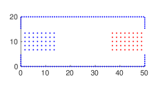
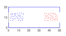
Fig. 1: Initial distribution of grid particles for the systematic distribution case (left) and the random distribution case (right).

5.1 Understanding decision-making phase

In this subsection we consider systematic and random initial distribution of 80 grid points (40 grid points on each end) as in figure 1. Pedestrians at left entrance have the destination point (50,10). The pedestrians entering at right entrance have (0,10) on the opposite end. Here we try to understand collision avoidance between particles by the comparison of without control on direction and with control on direction. In the case of without control on direction, pedestrians have only the information to satisfy goal (i.e. the angular velocity is given by (14) if the deviation to the goal is large, otherwise, zero). We use the constant time step $\Delta t=0.00042$, initial spacing of particles $\Delta x=1.68$ and $R=1.68$.

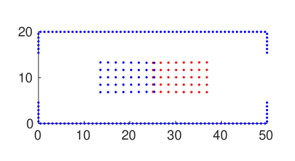
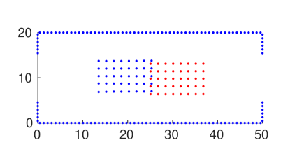
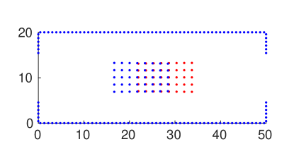
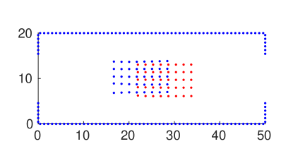
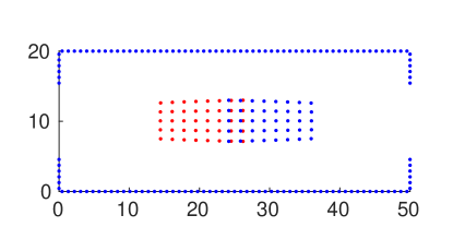
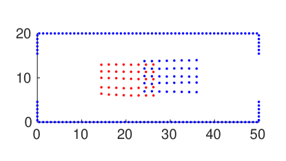
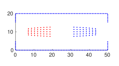
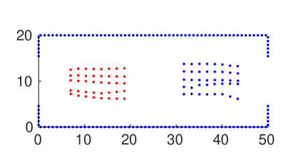
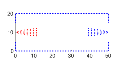
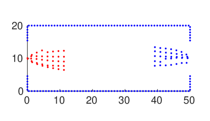
Fig. 2: Distribution of grid particles in the model without control on direction (first column) and with control on direction (second column) at time $t=8,10,15,20,25$ (top to bottom) respectively.

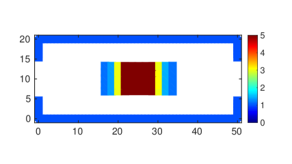
Fig. 3: Density of pedestrians in the model without control on direction (top) and with control on direction (bottom) at time $t=10$.

Figure 2 shows the time evolution of the grid particles in the model without control on direction (first column) and with control on direction (second column) at time $t=8$, $t=10$, $t=15$, $t=20$ and $t=25$. One observes that when grid particles are close to each other then they avoid collision by changing their direction. The results for the location of the grid points show similarities with those obtined in [3]. Figure 3 shows the corresponding density plots for the time $t=10$ in the model without control on direction (top) and with control on direction (bottom). The density is higher in case there is no control on direction.

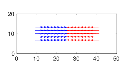
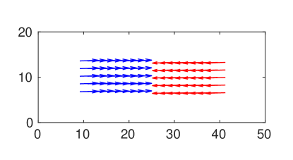
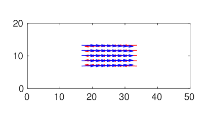
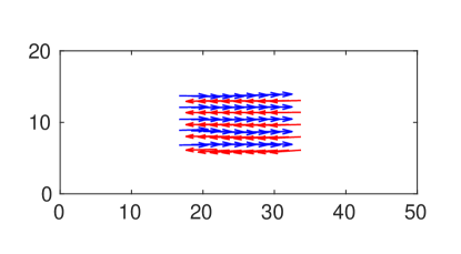
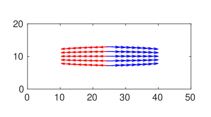
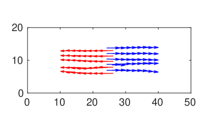
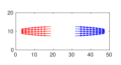
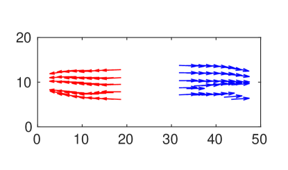
Fig. 4: Direction of grid particles in the model without control on direction (first column) and with control on direction (second column) at time $t=5,10,15,20$ (top to bottom) respectively.

Figure 4 shows the time evolution of particle paths in the model at time $t=5$, $t=10$, $t=15$ and $t=20$. One observes the change in the direction of particle paths when pedestrians are close to each other.

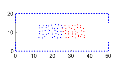
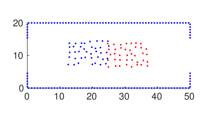
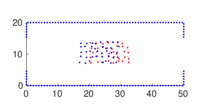
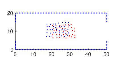
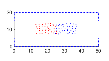
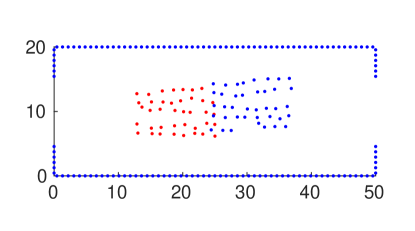
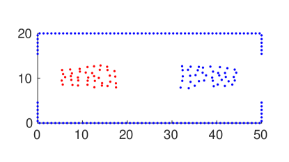
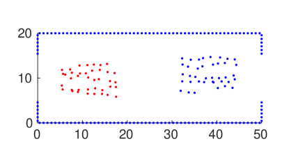
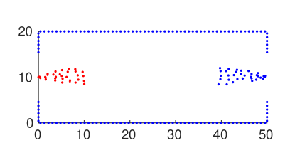
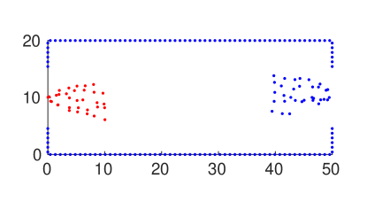
Fig. 5: Random distribution of grid particles in the model without control on direction (first column) and with control on direction (second column) at time $t=7.14,10,15,20,25$ (top to bottom) respectively.

In the earlier examples, we have initialized particles in a regular lattice. In real situations, the initial positions can be randomly distributed. Therefore, in figure 5 we consider the time evolution of randomly distributed grid particles in the model without control on direction (first column) and with control on direction (second column) at time $t=7.14$, $t=10$, $t=15$, $t=20$ and $t=25$. Again one observes the change in direction to avoid collision.

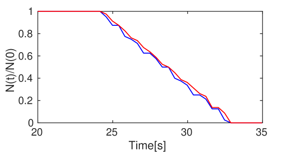
Fig. 6: Ratio of initial and actual grid particles with respect to time in the model without control on direction (blue) and with control on direction (red).

Figure 6 shows the percentage of grid particles being in the computational domain for the model without control on direction and with control on direction with respect to time. One observes that the evacuation time is almost similar in this simple case. However, it may differ for complicated and larger geometries.

5.2 Improvement of collision avoidance

If we decrease the initial spacing of the particles, then the particles might collide after interaction with other particles. So, in this subsection we improve collision avoidance between particles by adding some small extra repulsive force as in the social force model between particle in the vision-based model, for details of extra repulsive force we refer [4].

Here, we consider 100 grid points (50 gridpoints on each side having target at the opposite end). We use the constant time step $\Delta t=0.00021$, initial distance of grid points $\Delta x=0.84$ and $R=1.0$. For repulsive force between particles, we use the following values of parameters as $k_{n}=1.0$, $\gamma_{n}=0.01$ and $\gamma_{t}=0.01$.

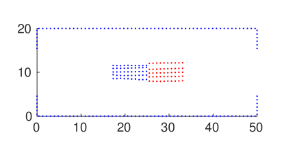
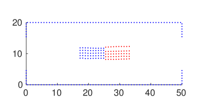
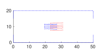
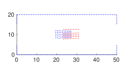
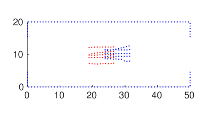
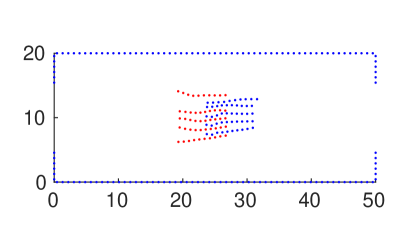
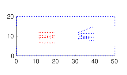
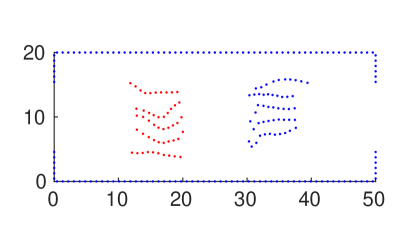
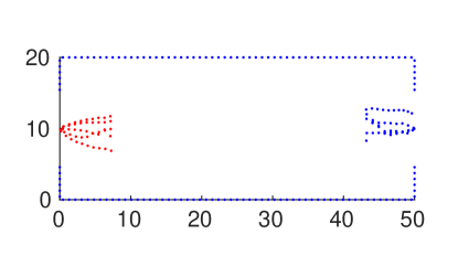
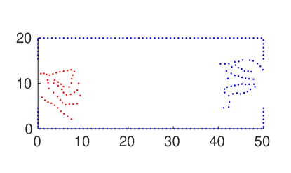
Fig. 7: Distribution of grid particles in the vision-based model (left column) and vision-based model with extra repulsion force (right column) at time $t=10.5,12,15,20,28$ (top to bottom).

Figure 7 shows the time evolution of the grid particles in the model without extra repulsive force between grid particles (left column) and with extra repulsive force between grid particles (right column) at time $t=10.5$, $t=12$, $t=15$, $t=20$ and $t=28$. If we do not use an additional repulsive force we can clearly observe that some particles collide with each other.

5.3 Comparison of non-local and local approximation

In this subsection we compare the non-local approximation with the local approximation for different $\lambda$. We use the same value of parameters as in subsection 5.1.

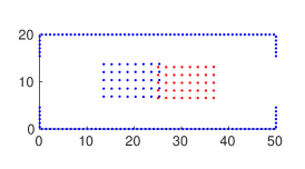
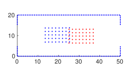
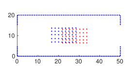
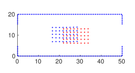
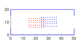
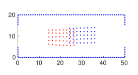
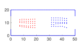
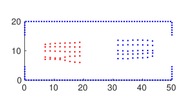
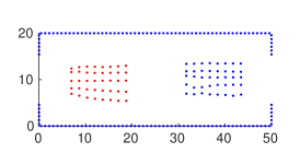
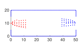
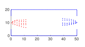
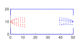
Fig. 8: Distribution of grid particles in non-local (first column) and local for $\lambda=10^{-2}$ (second column), $\lambda=10^{-5}$ (third column) at time $t=8,10,15,20,25$ (top to bottom) respectively.

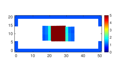
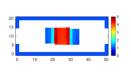
Fig. 9: Density of pedestrians in the model for non-local (top) and local approximations for $\lambda=10^{-2}$ (middle), $\lambda=10^{-5}$ (bottom) at time $t=10$.

Figure 8 shows the time evolution of the grid particles in non-local (first column), local for $\lambda=10^{-2}$ (second column) and local for $\lambda=10^{-5}$ (third column) at time $t=8$, $t=10$, $t=15$, $t=20$ and $t=25$. One observes that for $\lambda$ going to $0$, the the nonlocal approximation approaches the local model. Figure 9 shows the corresponding density plots at time $t=10$ in the models for non-local and local approximations, where the higher density in the center of geometry indicates more collisions of pedestrians.

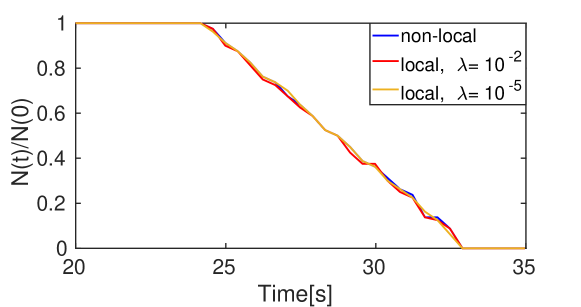
Fig. 10: Ratio of initial and actual grid particles with respect to time in non-local and local approximation of the model with different $\lambda$.

Figure 10 shows the percentage of grid particles being in the computational domain in non-local and local approximation of the model with different $\lambda$ with respect to time. In this case also, one observes that the evacuation time is similar in all models.

5.4 Comparison between vision-based pedestrian model and social force pedestrian model

In this subsection we consider the same parameters for the vision-based models as in section 5.1. We compare here the numerical simulation of the macroscopic vision-based pedestrian model and a social force based macroscopic pedestrian model which is coupled with the Eikonal equation. For details of the macroscopic social force model, we refer to [4]. Compare the results here also with the results obtained in [3] for the microscopic vision-based models.

For the social force model, we use the following values of parameters: $\Delta t=0.00042$, $\gamma_{n}=1.0$, $\gamma_{t}=0.2$, $T=0.001$, $u_{\max}=1.5$ $m/s$ and different values of repulsive force coefficient $k_{n}$ as 100, 500, 1000, 2000.

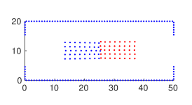
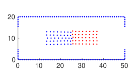
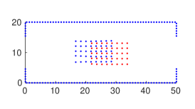
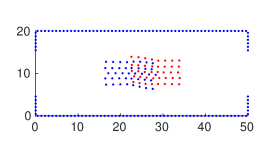
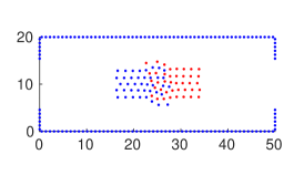
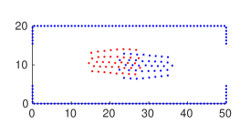
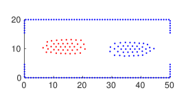
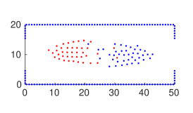
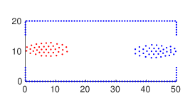
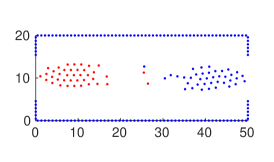
Fig. 11: Distribution of grid particles in the vision-based model (first column), social force model with $K_{n}=100$ (second column) and social force model with $K_{n}=1000$ (third column) at time $t=8,10,15,20,25$ (top to bottom).

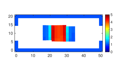
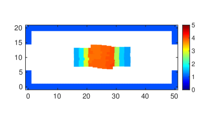
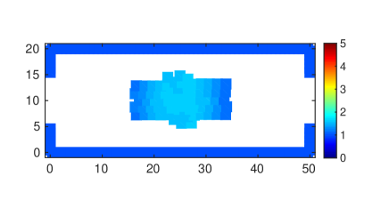
Fig. 12: Density of pedestrians in the vision-based model (top), social force model with $K_{n}=100$ (middle) and social force model with $K_{n}=1000$ (bottom) at time $t=10$.

Figure 11 shows the time evolution of the grid particles in vision-based model and social force pedestrian models for different $k_{n}$ at time $t=8$, $t=10$, $t=15$, $t=20$, and $t=25$. One can observe that collision avoidance between pedestrians of the vision-based model is almost similar with a social force pedestrian model for $k_{n}=100$. For bigger values of $k_{n}$ as in the third column of figure 11 one observes larger differences. Figure 12 shows the corresponding density plots at time $t=10$ in vision-based model and social force pedestrian models for different $k_{n}$.

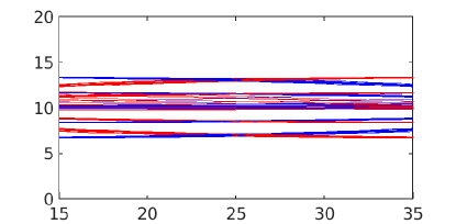
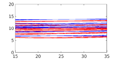
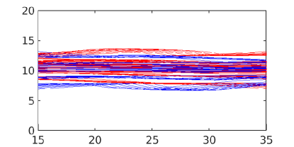
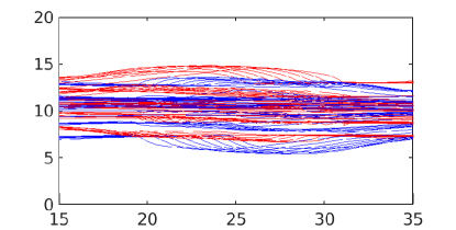
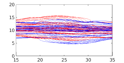
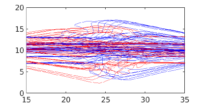
Fig. 13: Trajectory of the grid particles in the models such as vision-based model without control on direction (top left), vision-based model with control on direction (top right), social force model for $k_{n}$ being 100 (middle left), 500 (middle right), 1000 (bottom left), 2000 (bottom right) respectively.

Figure 13 shows the trajectory of the grid particles in the vision-based model and social force model. For larger values of $k_{n}$ in the social force model one observes trajectory which are similar to those obtained in [3].

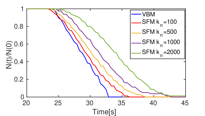
Fig. 14: Ratio of initial and actual grid particles with respect to time in vision-based model and social force model with different $k_{n}$.

Figure 14 shows the percentage of grid particles being in the computational domain for the vision-based model and social force model for the different $k_{n}$ with respect to time. One observes that the evacuation time is larger in the social force model and also, increasing for larger values of $k_{n}$.

5.5 Computational time

The computational time for a simulation of the macroscopic equation up to $t=45s$ are given for the vision-based model and the social force based model in table 1. One observes that the social force model has almost double the computational costs than the vision-based model. This is mainly due to the solution of the Eikonal equation with source depending on $\rho(t,x)$, which has to be solved at every time step.

Models	RUN TIME
VBM without control on direction	02:00
VBM with control on direction	02:01
Social force model with $k_{n}=100$	04:23
Social force model with $k_{n}=500$	04:29
Social force model with $k_{n}=1000$	04:31
Social force model with $k_{n}=2000$	04:35

Table 1: Computing time of the vision-based model and social force model.

6 Conclusion

We have considered the macroscopic vision-based pedestrian model presented in [2]. A mesh-free particle method to solve the governing equations is presented and used for the computation of several numerical examples analysing non-local and local vision-based model with and without additional social force terms. Also, we have presented a comparison between macroscopic models based on vision-based model and on social force pedestrian model coupled with the eikonal equation for a simple bi-directional situation. Results obtained here with a mesh free particle method for macroscopic equations are in accordance with the ones obtained for the microscopic vision based model in [3]. Future research topics are in particular the consideration of more complex situations, for example, interaction with moving objects and comparison with experimental data.

References

- [1]
- [2] Degond P., Appert-Rolland C., Petteré J., Theraulaz G., Vision-based macroscopic pedestrian models, Kinetic and Related models, AIMs 6(4), 809-839 (2013)
- [3] Ondřej J., Pettré J., Olivier A.H., Donikian S., A synthetic-vision based steering approach for crowd simulation, ACM Transactions on Graphics, 29(4), Article 123 (2010)
- [4] Etikyala R., Göttlich S., Klar A., Tiwari S., Particle methods for pedestrian flow models: From microscopic to nonlocal continuum models, Mathematical Models and Methods in Applied Sciences, 20(12), 2503-2523 (2014)
- [5] Reynolds C.W., Steering behaviors for autonomous characters, In the proceedings of Game Developers Conference, San Jose, California, 763-782 (1999)
- [6] Helbing D., Molnár P., Social force model for pedestrian dynamics, Phys. Rev. E, 51, 4282-4286 (1995)
- [7] Helbing D., Farkas I.J., Molnár P., Vicsek T., Simulation of pedestrian crowds in normal and evacuation situations, In: M. schreckenberg, s.d. sharma (eds.), Pedestrian and Evacuation Dynamics, Springer-Verlag, Berlin, 21-58 (2002)
- [8] Maury B., Roudneff-Chupin, Santambrogio F., A macroscopic crowd motion model of the gradient-flow type, Math. Models Methods Appl. Sci., 20, 1787-1921 (2010)
- [9] Piccoli B., Tosin A., Pedestrian flows in bounded domains with obstacles, Contin. Mech. Thermodynam., 21, 85-107 (2009)
- [10] Lemercier S., Jelic A., Kulpa R., Hua J., Fehrenbach J., Degond P., Appert-Rolland C., Donikian S., Pettré J., Realistic following behaviors for crowd simulation, Comput. Graph. Forum, 31, 489-498 (2012)
- [11] Burstedde C., Klauck K., Schadschneider A., Zittartz J., Simulation of pedestrian dynamics using a two-dimensional cellular automaton, Physica A, 295, 507-525 (2001)
- [12] Luo L., Fu Z., Cheng H., Yang L., Update schemes of multi-velocity floor field cellular automaton for pedestrian dynamics, In the proceedings of Game Developers Conference, 491, 946-963 (2018)
- [13] Karbovskii V., Voloshin D., Karsakov A.B.A., Gershenson C., Multi-model agent-based simulation environment for mass-gatherings and pedestrian dynamics, Future Generation Computer Systems, 79, 155-165 (2018)
- [14] Omer I., Kaplan N., Using space syntax and agent-based approaches for modeling pedestrian volume at the urban scale, Computers, Environment and Urban Systems, 64, 57-67 (2017)
- [15] Hoogendoorn S., Bovy P.H.L., Simulation of pedestrian flows by optimal control and differential games, Optimal Control Appl. and Methods, 24, 153-172 (2003)
- [16] Helbing D., A mathematical model for the behavior of pedestrians, Behav. Sci., 36, 298-310 (1991)
- [17] Helbing D., Molnár P., Self-organization phenomena in pedestrian crowds, In: Schweitzer, F.(ed.) Self-Organization of Complex Structures: From Individuals to Collective Dynamics, 567-577. Gordon and Breach, London (1997)
- [18] Hughes R., Ondřej J., Dingliana J., Davis: Density-adaptive synthetic vision based steering for virtual crowds, Proceedings of the 8th ACM SIGGRAPH Conference on Motion in Games, 79-84 (2015)
- [19] Guy S.J., Chhugani J., Kim C., Satish N., Lin M., Manocha D., Dubey P., Clearpath: Highly parallel collision avoidance for multi-agent simulation, In: ACM SIGGRAPH/Eurographics Symposium on Computer Animation, 177-187 (2009)
- [20] Huang W.H., Fajen B.R., Fink J.R., Warren W.H., Visual navigation and obstacle avoidance using a steering potential function, Robot. Auton. Syst., 54, 288-299 (2006)
- [21] Paris S., Pettré J., Donikian S., Pedestrian reactive navigation for crowd simulation: a predictive approach, Eurographics, 26, 665-674 (2007)
- [22] PettréJ., Ondřej J., Olivier A.H., Cretual A., Donikian S., Experiment-based modeling, simulation and validation of interactions between virtual walkers, In: SCA ’09: Proceedings of the 2009 ACM SIGGRAPH/Eurographics Symposium on Computer Animation, 189-198 (2009)
- [23] Berg J. van den, Overmars H., Planning time-minimal safe paths amidst unpredictably moving obstacles, Int. J. Robot. Res., 27, 1274-1294 (2008)
- [24] Mahato N.K., Klar A., Tiwari S., Particle methods for multi-group pedestrian flow, Applied Mathematical Modelling, 53, 447-461 (2018)
- [25] Degond P., Appert-Rolland C., Moussaïd M., Petteré J., Theraulaz G., A hierarchy of heuristic-based models of crowd dynamics, J. Stat Phys, 152, 1033-1068 (2013)
- [26] Bellomo N., Dogbe C., On the modeling crowd dynamics from scaling to hyperbolic macroscopic models, Math. Models Methods Appl. Sci., 18, 1317-1345 (2008)
- [27] Helbing D., A fluid dynamic model for the movement of pedestrians, Complex Syst., 6, 391-415 (1992)
- [28] Treuille A., Cooper S., Popovic Z., Continuum crowds, ACM Transactions on Graphics (proceedings of the “SIGGRAPH 2006” conference), 25
- [29] Cutting J.E., Vishton P.M., Braren P.A., How we avoid collisions with stationary and moving objects., Phychol. Rev., 102, 627-651 (1995)
- [30] Warren W.H., Fajen B.R., From optic flow to laws of control, In: Vaina L.M., Beardsley S.A., Rushton S.K. (eds) Optic Flow and Beyond, 324, 307-337. Springer, Dordrecht (2004)
- [31] Moussaïd M., Helbing D., Theraulaz G., How simple rules determine pedestrian behavior and crowd disasters, Proc. Natl. Acad. Sci. USA, 108, 6884-6888 (2011)
- [32] Tiwari S., Kuhnert J., Modelling of two-phase flow with surface tension by finite pointset method (fpm), J. Comp. Appl. Math, 203, 376-386 (2007)
- [33] Tiwari S., Kuhnert J., Finite pointset method based on the projection method for simulations of the incompressible navier-stokes equations, Meshfree Methods for Partial Differential Equations, eds. M. Griebel and M.A. Schweitzer, Lecture Notes in Computational Science and Engineering, 26, 373-387. Springer-Verlag (2003)