Coupled Wire Model of $Z_{4}$ Orbifold Quantum Hall States

Abstract

We introduce a coupled wire model for a sequence of non-Abelian quantum Hall states that generalize the $Z_{4}$ parafermion Read Rezayi state. The $Z_{4}$ orbifold quantum Hall states occur at filling factors $\nu=2/(2m-p)$ for odd integers $m$ and $p$, and have a topological order with a neutral sector characterized by the orbifold conformal field theory with central charge $c=1$ at radius $R=\sqrt{p/2}$. When $p=1$ the state is Abelian. The state with $p=3$ is the $Z_{4}$ Read Rezayi state, and the series of $p\geq 3$ defines a sequence of non-Abelian states that resembles the Laughlin sequence. Our model is based on clustering of electrons in groups of four, and is formulated as a two fluid model in which each wire exhibits two phases: a weak clustered phase, where charge $e$ electrons coexist with charge $4e$ bosons and a strong clustered phase where the electrons are strongly bound in groups of 4. The transition between these two phases on a wire is mapped to the critical point of the 4 state clock model, which in turn is described by the orbifold conformal field theory. For an array of wires coupled in the presence of a perpendicular magnetic field, strongly clustered wires form a charge $4e$ bosonic Laughlin state with a chiral charge mode at the edge, but no neutral mode and a gap for single electrons. Coupled wires near the critical state form quantum Hall states with a gapless neutral mode described by the orbifold theory. The coupled wire approach allows us to employ the Abelian bosonization technique to fully analyze the physics of single wire, and then to extract most topological properties of the resulting non-Abelian quantum Hall states. These include the list of quasiparticles, their fusion rules, the correspondence between bulk quasiparticles and edge topological sectors, and most of the phases associated with quasiparticles winding one another.

I Introduction

Recent works have studied the two dimensional quantum Hall effect as a set of coupled planar parallel quantum wires subject to a perpendicular magnetic fieldKane et al. (2002); Teo and Kane (2014); Neupert et al. (2014); Klinovaja and Tserkovnyak (2014); Sagi and Oreg (2014); Santos et al. (2015); Meng et al. (2015); Sagi and Oreg (2015); Huang et al. (2016); Iadecola et al. (2016); Mross et al. (2015, 2016); Klinovaja et al. (2016); Fuji and Lecheminant (2017). The easiest case to consider is that of the integer quantum Hall effect, where interactions between electrons are not essential. The fractional quantum Hall states require interactions, and the coupled wire description enables the application of bosonization techniquesHaldane (1981a, b) for the analysis of these interactions. As expected, among the fractional quantum Hall states the Laughlin $\nu=1/m$ “magic fractions”Laughlin (1983) are easiest to handle, with the complexity increasing when dealing with hierarchy states. The non-Abelian quantum Hall, including the Moore Read stateMoore and Read (1991) and Read Rezayi states statesRead and Rezayi (1999) were reproduced by coupled wire constructionsTeo and Kane (2014), but at the cost of introducing a spatially modulated magnetic field.

In our earlier paperKane et al. (2017), to which the present paper is a companion, we showed how to use a coupled wire model to construct non-Abelian states that are a result of clustering of electrons into pairs. These states, of which the best known is the Moore-Read Pfaffian stateMoore and Read (1991), may also be described as various types of $p$-wave superconductors of Chern-Simons composite fermionsRead and Green (2000). Our construction combined the two ingredients common to all Read-Rezayi non-Abelian quantum Hall states: the clustering of electrons (in this case into pairs) and the construction of an edge made of a chiral charge mode that is a Luttinger liquid and a chiral neutral mode that is described by a Conformal Field Theory (CFT) of a fractional central charge. It did not require a modulated magnetic field.

In this work we focus on another set of non-Abelian states, in which electrons cluster to groups of four, and the neutral edge mode is described in terms of an orbifold theoryDi Francesco et al. (1997); Ginsparg (1988a). The Read-Rezayi series of non-Abelian statesRead and Rezayi (1999) is based on the construction of clusters of $k$-electrons at filling factors $\nu=k/(mk+2)$ (with $m$ odd) or the clustering of $k$-bosons at $\nu=k/(mk+2)$ (with $m$ even). In both cases it may be viewed as a Bose condensate of these clusters, which, due to Chern-Simons flux attachment, may be mapped onto Bosons at zero magnetic field. The Read-Rezayi series span all positive integer values of $k$.

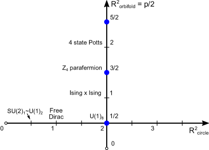
Figure 1: Conformal field theories with $c=1$ include two intersecting lines of continuously varying critical pointsGinsparg (1988b, a). The horizontal line describes a free boson compactified on a circle of radius $R_{\rm circle}$, while the vertical line describes a free boson compactified on an orbifold of radius $R_{\rm orbifold}$Note (1). The circle theory at $R_{\rm circle}=\sqrt{2}$ and the orbifold theory at $R_{\rm orbifold}=1/\sqrt{2}$ are equivalent and related by an $SU(2)$ symmetry. The $Z_{4}$ orbifold states studied in this paper form a sequence analogous to the Laughlin sequence, and have edge states with a neutral sector described by the orbifold theory at $R_{\rm orbifold}=\sqrt{p/2}$, where $p$ is an odd integer, indicated by the solid blue circles.

The case of $k=4$ is unique. On one hand, it is too complicated to allow for a quadratic mean field Hamiltonian description. On the other hand, we show here that it does allow for a rather detailed and transparent analysis of its many-body Hamiltonian. Our work highlights the connection between the coupled wire model and the $c=1$ orbifold theory developed by Dijkgraaf, Vafa, Verlinde and VerlindeDijkgraaf et al. (1989), which formed the basis for the analysis of orbifold quantum Hall states carried out by Barkeshli and WenBarkeshli and Wen (2011).

The space of conformal field theories with $c=1$ was studied extensively in the 1980’sGinsparg (1988b, a); Dijkgraaf et al. (1989); Di Francesco et al. (1997), and has the structure depicted in Fig. 1. It includes two intersecting lines of continuously varying critical points, denoted the “circle” line and the “orbifold” line. The circle line is equivalent to the theory of an ordinary single channel Luttinger liquid, which can be described as a free boson $\varphi$ with Lagrangian density $(\partial_{\mu}\varphi)^{2}/8\pi$ compactified on a circle, so that $\varphi\equiv\varphi+2\pi R_{\rm circle}$. The radius $R_{\rm circle}$ is related to the Luttinger parameter $K$, and specific radii describe rational CFT’s of interest. The value $R_{\rm circle}=1/\sqrt{2}$ is the theory of the spin sector of $SU(2)$ fermions, described by $SU(2)_{1}$, or equivalently $U(1)_{2}$, with $K=2$. The edge states of bosonic Laughlin states at filling $\nu=1/m$ with $m$ even are described by $R_{\rm circle}=\sqrt{m}/2$. Fermionic Laughlin states at $\nu=1/m$ are described by the circle theory at $R_{\rm circle}=\sqrt{m}$ with a constrained Hilbert space. In particular, for $\nu=1$, the free Dirac fermion is at $R_{\rm circle}=1$.

The orbifold theory is a variant on the Luttinger liquid model, and describes a free boson compactified on a circle with radius $R_{\rm orbifold}$ in which angles $\theta$ and $-\theta$ are identified. The orbifold theory at $R_{\rm orbifold}=1/\sqrt{2}$ and the circle theory at $R_{\rm circle}=\sqrt{2}$ (describing $U(1)_{8}$ - or $K=8$) are equivalent and are related by a hidden $SU(2)$ symmetry, which will play a key role in our analysis. The orbifold theory at specific radii correspond to theories of interest, including doubled Ising model at $R_{\rm orbifold}=1$, the $Z_{4}$ parafermion CFT at $R_{\rm orbifold}=\sqrt{3/2}$ and the 4 state Potts model at $R_{\rm orbifold}=\sqrt{2}$.

The $Z_{4}$ orbifold states that we will construct in this paper occur at filling factors

$$\nu=\frac{2}{2m-p}$$ (1)

where $m$ and $p$ are odd integers. They have neutral edge modes that are described by the orbifold CFT at $R_{\rm orbifold}=\sqrt{p/2}$. When $p=1$, the state is Abelian, and has an alternate description in terms of the circle CFT. When $p=3$ the orbifold state is equivalent to the $Z_{4}$ parafermion Read Rezayi state. Our coupled wire formulation takes advantage of the $SU(2)$ symmetry mentioned above, which allows for a description of the orbifold CFT in terms of Abelian bosonization. This highlights the similarity between the sequence of orbifold states states for $p=1,3,5,...$ and the Laughlin sequence of Abelian states at $\nu=1/m$, and allows a rather detailed analysis of the topological structure of the ground state and quasiparticle excitations.

The rest of the paper presents our analysis. Sec. (II) presents our results and the physical picture that we develop to understand them. Sec. (III) analyzes a single wire where the interaction between electrons favors a clustering to $k$ electrons. Sec. (IV) focuses on the case $k=4$ and shows how this case may be solved by exploiting a hidden $SU(2)$ symmetry. Section (V) constructs quantum Hall states from single wires of the type discussed in Sec. (IV). Sec. (VI) analyzes the quasi-particles of these states, and Sec. (VII) gives a concluding discussion.

II Physical picture and summary of results

II.1 Single Wire

II.1.1 General set-up

Our approach for creating a coupled wire description of the $k=4$ states is similar to our earlier construction of $k=2$ statesKane et al. (2017). It is a two-fluid model, both of the single wire and of the entire system. For each wire we start with two pairs of counter-propagating gapless modes: one carries clusters of four electrons and is described by the fields $\varphi_{4},\theta_{4}$; the other carries single electrons and is described by the fields $\phi_{1L},\phi_{1R}$. We then introduce two interaction terms, one ($u$) that back-scatters single electrons and one ($v$) that composes and decomposes clusters into four electrons. The Hamiltonian density for a single wire then takes the form

$${\cal H}={\cal H}_{0}+{\cal H}_{int}$$ (2)

where ${\cal H}_{0}$ is the Luttinger liquid Hamiltonian density for the two pairs of fields, and the interaction Hamiltonian density is

$${\cal H}_{int}=u\cos{(\varphi_{4}-2\phi_{1L}-2\phi_{1R})}+v\cos{(\phi_{1R}-\phi_{1L})}$$ (3)

When the second interaction term dominates there is an energy gap for single electron excitations, and the system is in a strongly clustered state. It carries a pair of counter-propagating gapless cluster modes. When the first term dominates the single wire is in a weakly-clustered state in which one of the two pairs of counter-propagating modes is gapped. In this state there is no energy gap for single electron excitations. The operator that inserts a single electron with a vanishing energy cost does so with the insertion of a winding to the phase of the bosonic phase field of the clusters. Finally, in between these two phases there is a critical state in which none of the modes is gappedLecheminant et al. (2002).

II.1.2 A wire at the critical state

The nature of the critical state is what makes the $k=4$ state unique when compared to $k=2,3$. While for $k=2,3$ there is a single critical point, for $k=4$ there is a critical line, i.e., the low energy properties depend on the value of $u$ and $v$. Furthermore, while for $k=2,3$ the central charge of the gapless state is fractional, for $k=4$ it is an integer.

For the $k=4$ case the competition of the $u,v$ terms in (3) is reminiscent of the quantum four-state clock-modelFradkin and Kadanoff (1980), composed of one dimensional lattice of “clocks”. This model is a special case of the more general Ashkin-Teller modelGinsparg (1988a); Di Francesco et al. (1997), which has recently appeared in a number of contexts Lecheminant et al. (2002); Zhang and Kane (2014); Kane and Zhang (2015); Meidan et al. (2017). In this model each site hosts a phase degree of freedom $\phi_{i}$. An interaction term assigns an energy cost $\sim\cos{4(\phi_{i}-\phi_{i+1})}$ to a phase difference between neighboring site, while an on-site term introduces a change of the local phase $\phi_{i}\rightarrow\phi_{i}\pm\frac{\pi}{2}$. The relative size of these terms determines whether the system is in an ordered or disordered phase. As we describe below, the critical state of the single wire of our problem has much similarity with the critical state of the Ashkin-Teller model. Like the latter, its low energy spectrum includes an orbifold theory of central charge $c=1$, whose properties are analyzed in detail in Ref. Dijkgraaf et al., 1989.

Our focus here is on wires in the critical state. For all values of $k$ the kinetic energy of the two counter-propagating pairs of modes is quadratic in the bosonic fields that describe the modes, while the two competing interaction terms are cosines of combinations of the bosonic fields, which do not commute with one another. The non-commutativity of the interaction terms makes the Hamiltonian generally difficult to handle. For $k=2$ the fermionic language comes to the rescue, since the interaction turns out to be quadratic in terms of properly chosen Majorana fermions. For $k=4$ the interaction terms are not quadratic. However, the $k=4$ case has a hidden $SU(2)$ symmetry, which is not apparent in Eq. (3). Due to that symmetry, a properly chosen fermionic representation allows for an expression of the interactions as interactions of small momentum transfer, which allows for their mapping onto a quadratic Luttinger liquid. The nature of the mapping imposes constraints on the Luttinger liquid, and these constraints translate into an orbifold theory.

Our study hops between the fermionic and bosonic representation of the one dimensional degrees of freedom that we analyze. The bosonization approach to one dimensional systems allows for the definition of vertex operators of the form $e^{i{\bf\alpha\cdot\phi}}$ where ${\bf\phi}\equiv\left(\phi_{e,R},\phi_{e,L},\phi_{4},\theta_{4}\right)^{T}$ is the vector of bosonic fields that describe the system and $\bf\alpha$ is a vector of real numbers. The value of $\bf\alpha$ determines the quantum statistics of the operator. When the components of $\alpha$ are all integers, the operator is local, i.e., it is composed of creation and annihilation operators of single electrons and four-electron clusters within a localized region. All operators within a Hamiltonian must obviously be local. In the case we consider, where the starting point is that of two pairs of counter-propagating bosons, the hidden $SU(2)$ symmetry is brought to the forefront by choosing a set of four vectors $\bf\alpha$ that express the problem in terms of two types of fermions, each having left and right moving branches. When we assign the two types of fermions a fictitious spin “up”/“down”, any operator that involves the two types of fermions takes the form of a spin-$1/2$ field. From here on we will use the term spin freely, referring always to the fictitious spin. We will refer to these newly defined fermions as “the $SU(2)$ fermions”, to distinguish them from the original (spinless) electronic degrees of freedom. The one dimensional $SU(2)$ fermions may be described by two pairs of counter propagating bosonic modes, which we denote by $\phi_{s,a}$, with $s=\uparrow,\downarrow$ denoting the spin direction and $a=L,R$ denoting the direction of motion.

The expression of the original degrees of freedom in terms of $SU(2)$ fermions is possible for all values of $k$. It is useful for $k=4$ due to three unique characteristicsLecheminant et al. (2002); Ginsparg (1988a). First, there is a simple criterion that determines whether an operator expressed in terms of the $SU(2)$ fermions is local in terms of the original electrons. This criterion states that a local operator is an operator that changes the number of spin-down fermions by an even number. Thus, the physical subspace of the Hilbert space of the $SU(2)$ fermions is constrained to the states at which the number of down fermions is even, and the local operators commute with the parity of the number of spin-down fermions. Second, many of the operators that are local in terms of the original electrons turn out to be local also in terms of the $SU(2)$ fermions (exceptions will be elaborated on below). And third, at the critical point the Hamiltonian takes a particularly simple form in terms of the $SU(2)$ fermions. The kinetic term is an isotropic ferromagnetic coupling which does not mix different chiralities. It is quadratic in the $\phi_{s,a}$’s. The critical interaction term couples the $x$-components of the spins of right and left moving $SU(2)$ fermions to one another. So, not only is the Hamiltonian local with respect to the fermions, it is also in a form that may be diagonalized. Its diagonalization, however, requires us to bosonize the $SU(2)$ fermions, since the Hamiltonian is quartic in $SU(2)$ fermion operators.

In the bosonized language of the $SU(2)$ fermions, the $x,y$-components of the spin density are non-linear in the bosonic fields $\phi_{s,a}$, involving factors such as $S^{\pm}\sim\exp{\pm i(\phi_{a,\uparrow}-\phi_{a,\downarrow})}$. In contrast, the $z$-component is linear, involving only $S_{z}\sim\partial_{x}(\varphi_{a,\uparrow}-\varphi_{a,\downarrow})$. Consequently, it is desirable to rotate the spin axes by $\pi/2$ around the $y$-axis, such that the coupling of $x$-components of the right- and left-moving spins becomes a coupling of the $z$-components. Were it not for the constraint imposed on the physical subspace, this would have been just a renaming of axes. However, the rotation affects also the constraint, transforming it to the statement that in the rotated frame a local operator is an operator that is invariant to the interchange of spin-up with spin-down fermions.

When the transformation from the original degrees of freedom to the rotated fermions is completed, the effect of the critical interaction is to transform the two pairs of counter-propagating bosonic modes, of the clusters and the single electrons, into two pairs of coupled counter-propagating modes, of the spin-up and down $SU(2)$ fermions, subjected to a constraint on the allowed operators and allowed states. The gapless modes of the rotated fermions can then be described by a third and last set of bosonic fields $\chi^{r}_{\rho,a}$ and $\chi^{r}_{\sigma,a}$, where the super-script $r$ indicates the rotated frame, the subscripts $\rho,\sigma$ indicate charge and spin fields, and the subscript $a$ indicates again a direction of motion. The Hamiltonian is quadratic in these fields, and the interaction term couples only the spin fields. The Hamiltonian is diagonalized to a pair of counter-propagating charge modes and a pair of counter-propagating spin modes, with the only parameter in the diagonalization being the relative strength of the critical interaction to the kinetic term. This parameter determines the relative velocity of the charge and spin modes, as well as the eigen-operators of the spin mode. The eigenmodes mix the right- and left-moving fermions of the non-interacting problem to create chiral eigenmodes of the interacting one. There is a set of discrete values of the critical interaction parameter $\lambda$ for which the eigen-operators of the spin modes create an integer number $p$ fermions of one chirality and $p-1$ fermions of the opposite chirality. This discrete set of $\lambda$’s play a special role below. The most obvious example is the non-interacting case, $\lambda=0$, for which $p=1$. Operators are local when they are invariant to the transformation $\chi^{r}_{\sigma,a}\rightarrow-\chi^{r}_{\sigma,a}$ for both $a=R,L$. The charge mode is not affected by this constraint.

As mentioned before, the transformation from the four electron clusters and single electrons to the $SU(2)$ fermions has the virtue that almost all local operators in the original degrees of freedom correspond to local degrees of freedom in the fermionic representation. Notable exceptions are the operators $e^{i(2n+1)\theta_{4}}$, with an integer $n$. In the original degrees of freedom, the $n=0$ operator is an operator that introduces a $2\pi$ kink into the field $\phi_{4}$. When expressed in terms of the $SU(2)$ fermions, it becomes an operator that introduces a $\pi$ kink into the spin field of the fermions.

II.2 From coupled wires to a quantum Hall state

Tunneling between wires forms a quantum Hall state when it gaps the gapless modes in the bulk and leaves gapless chiral modes near the edgeKane et al. (2002); Teo and Kane (2014). In an idealized situation, that would happen when the tunneling operator couples only left movers of one wire to right movers of a neighboring wire. In the present case each wire has two counter-propagating pairs of modes. In the strong-clustered and weak-clustered phases one of these pairs is gapped by intra-wire interactions, such that inter-wire tunneling needs to gap only one pair. In the critical state, however, two tunneling terms are needed to gap the two pairs of gapless modes.

To be effective, the tunneling terms should satisfy several conditions: there must be a spectral weight for the tunneling particle to tunnel into or out of a wire at the chemical potential; the tunneling particle must be local; and there must be a momentum balance. The sum of the momentum that the tunneling particle takes from its wire of origin and the momentum that it receives from the Lorenz force when it tunnels should equal the momentum that is associated with the state to which it tunnels in the wire of destination. These requirements are general to all wire constructions of quantum Hall states, but some aspects of their application are unique to the present context.

The identity of the particles that have a spectral weight to tunnel at the chemical potential depends on the phase that the single wire is in. In the strongly clustered states, the only particles that may tunnel are clusters of four electrons, which in the $SU(2)$ language are described as two spin-up and two spin-down fermions. Thus, each cluster is spinless. In the critical state all particles can tunnel at the chemical potential.

The notion of locality appears here twice. The tunneling particle must be local in terms of the electrons and the 4-electron clusters. However, it does not have to be local in terms of the $SU(2)$ fermions, which are calculational constructs. It is to be expected, though, that tunneling terms that are local also in terms of the $SU(2)$ fermions would be easier to analyze. Indeed, we study quantum Hall states based on such terms here, and defer those for which the tunneling terms are non-local in terms of the $SU(2)$ fermions to a future publication.

The balance of momentum is the major factor that determines the filling factors for which quantum Hall states are formed. The filling factors formed are those for which when a charge $q$ tunnels between states at the chemical potential on different wires, the momentum it adds to the electronic system in the wires equals the momentum it receives from the Lorenz force, namely $qBd$, where $d$ is the inter-wire distance. For $\nu=1$, for example, a single electron tunnels between two Fermi points, such that $eBd=2k_{F}=2\pi n_{e}$, which corresponds to $\nu=1$ (here $n_{e}$ is the one-dimensional electron density). When the tunneling event is accompanied by two intra-wire $2k_{F}$ scattering events, one in each of the participating wires, the momentum balance is $eBd=6k_{F}$, and the $\nu=1/3$ state is obtained.

For the present problem the condition for momentum balance depends on the identity of the tunneling particle, which depends on the state of the individual wires. Tunneling operators of 4-clusters have the form

$$e^{i\left(\varphi_{4}+L\theta_{4}+M(\phi_{1R}-\phi_{1L})\right)}$$ (4)

Here and below $L,M$ are integers, and $n_{b}$ is the number density of the bosonic clusters. These operators involve a momentum of $2\pi(Ln_{b}+Mn_{e})$. When the wires are in the strongly clustered phase, the only active degrees of freedom are the bosonic $4e$ clusters, such that $M=0$. Based on tunneling operators with $L=l$ Laughlin states of cluster filling factor $\nu_{4e}=1/{2l}$ may be formed, which correspond to electronic filling factors of $\nu=8/l$. The states are Abelian, and the edge carries a single chiral mode, with a central charge of one.

When the wires are in their critical states there are two tunneling processes, aimed at gapping the charge and the neutral modes. The charge mode is gapped by the same operator that gaps it in the strongly clustered state - a tunneling of a four-electron cluster, which corresponds to the tunneling of two spin-up and two spin-down $SU(2)$ fermions. The charge mode is insensitive to the interaction strength $\lambda$, and hence so is also the operator that gaps it.

The operator that gaps the spin mode must tunnel charge, so that it may get momentum from the Lorenz force, and must carry spin, to couple to the spin mode. A single electron tunneling is then the natural candidate. Generally, the single electron tunneling operator is

$$e^{i\left(\frac{1+m}{2}\phi_{1R}+\frac{1-m}{2}\phi_{1L}+l\theta_{k}\right)}.$$ (5)

with $m$ being an odd integer, and $l$ an integer. The momentum involved is $2\pi(mn_{e}+ln_{b})$. Close to the transition $n_{b}\gg n_{e}$, such that $4en_{b}$ is approximately the total charge density, and the momentum balance condition $2\pi ln_{b}=eBd$ translates to $\nu=2/l$. Furthermore, when expressed in terms of the $SU(2)$ fermions, the operators (5) are local only for odd $l$, imposing the final restriction on our analysis to filling factors of the form $\nu=2/l$, with odd $l$.

The momentum balance, and hence the filling factor, do not depend on the value of $m$ in (5). This value is determined by the requirement that the single electron tunneling term gaps the spin mode. Since the eigenvectors of the spin mode couple right- and left-moving electrons in a way that depends on the interaction scale $\lambda$, the tunneling operator should depend on the interaction as well. As explained before, for a set of discrete value $\lambda(p)$ there is a single electron operator that couples only to one chirality of the spin mode. For odd $p$, this happens when $m=(l+p)/2$.

Expressing $l$ in terms of $m$ and $p$, we summarize this subsection by saying that the analysis we present in this paper takes us from the Abelian quantum Hall states at $\nu=2/(2m-p)$, which are formed by wires at their strongly clustered phase, to quantum Hall states at the same $\nu$ formed by wires at their critical phase. The phase boundary between the two states is determined by the ratio of intra-wire single electron back scattering and inter-wire single electron tunneling. As we explain in the next subsection, the latter states are non-Abelian.

As a final remark on the subject we note that when the wires are in their weakly clustered phase, single electron tunneling may lead to the formation of an anisotropic quantum Hall state. A chiral charge mode then runs along the entire edge, and a neutral achiral edge mode exists along edges that are not parallel to the wires. The properties of this state are quite similar to those of its $k=2$ counterpartKane et al. (2017).

II.3 Topological properties of the quantum Hall states

The fractionalized quasiparticles of fractional quantum Hall states are manifested in the ground state degeneracy in a torus geometry, in the different topological sectors of the chiral edge modes in an annular geometry, and as gapped bulk excitations. Within the wire construction, the first two manifestations are expressed in terms of operators that create quasiparticle-quasihole pairs and position them on the two edges of the annulus or take them around the torus. The bulk quasiparticle-quasihole pair occurs as a kink-antikink pair in a bosonic phase variable that is pinned to one of several degenerate values in the system’s bulkKane et al. (2002); Teo and Kane (2014). In Sec. (VI) we analyze both edge and bulk quasiparticles. Here we describe the physical picture of bulk quasi-particles. We do so using the language of the $SU(2)$ fermions in the rotated system of axes.

The quasiparticle content of the strongly clustered quantum Hall states is rather easy to understand. The states we consider here are Laughlin states of 4-electrons clusters with the cluster filling factors being $1/8l$, and $l$ being odd integer. Their $K$-matrix is the number $8l$, and their charge vector is the number $4$. As such, they carry $8l$ fractionally-charged quasi-particles of charges $Q/2l$, with $Q=1,...,8l$. Within the wire construction, single electron backscattering in each wire gaps the spin degree of freedom and makes it irrelevant to the quantum Hall physics, while cluster tunneling between neighboring wires gaps the charge degrees of freedom, except one chiral mode at each edge. Within a bosonized description of the $SU(2)$ fermions, cluster tunneling leads to the pinning of a particular relative phase of the charge modes of neighboring wires, which we denote by ${\bar{\theta}}_{\rho}$ and define precisely in Eq. (89). This relative phase is pinned to one of $8l$ possible values for which the energy is minimal and degenerate. The quasi-particles reside between wires, in the form of kinks in the pinned relative phase. The charge $Q$ of the quasi-particle is coupled then to the phase jump between the start point and the end point of the kink, which is ${\bar{\theta}}_{\rho}=Q\pi/4l$.

When the quantum Hall state is formed of wires at the critical state the spin modes are gapped by single electron tunneling terms between neighboring wires. These terms involve both the charge and the spin modes, and couple them in an interesting way: when ${\bar{\theta}}_{\rho}$ is pinned to $j\pi/4l$ with an even value of $j$, it pins a relative phase of the spin sector ${\bar{\theta}}_{\sigma}$ (defined precisely in Eq. (104)) to one of $p$ possible values which are evenly spaced. When the value of $j$ is odd, a different relative phase ${\bar{\varphi}}_{\sigma}$ (defined precisely in Eq. (104)) is pinned to one of $p$ values which are evenly spaced. The two phases ${\bar{\varphi}}_{\sigma},{\bar{\theta}}_{\sigma}$ do not commute with one another. As a consequence, kinks in ${\bar{\theta}}_{\rho}$ of even $j$ may come together with kinks in the pinned spin phase, be it ${\bar{\varphi}}_{\sigma}$ or ${\bar{\theta}}_{\sigma}$. In contrast, kinks of odd $j$ come together with an excitation similar to the one occurring when two counter propagating FQHE edge modes are gapped alternately by a superconductor and by backscatteringLindner et al. (2012); J Clarke et al. (2013); Vaezi (2014); Cheng (2012); Mong et al. (2014). The appearance of this excitation makes the quasiparticle associated with an odd value of $j$ non-Abelian for all values of $p>1$. Excitations of this type will be referred to as a twist fields, and will be denoted by $\sigma,\tau$.

The interface between two regions with pinned non-commuting phase variables is one of two sources for non-Abelian quasiparticles. The other source is the constraint imposed on the Hilbert space of the $SU(2)$ fermions. In the rotated basis, physical states should be invariant to the interchange of spin-up and spin-down fermions. This interchange may be expressed as a transformation on the values of the bosonic phases ${\bar{\varphi}}_{\sigma},{\bar{\theta}}_{\sigma}$. The values to which each of these phases may be pinned are either invariant under the transformation or form pairs that are transformed onto one another. In the former case the states are allowed. In the latter case, which happens only for $p\geq 2$, they may occur only as superpositions of states pinned to the members of the pair. In these cases a phase variable is in a superposition of two distinct values over distances that may be macroscopic, the distances between a kink and its inverse. The superposition is protected from decoherence by the constraint, which makes operators that may distinguish the two superposed values unphysical. Again, a quasiparticle is a kink that separates between two regions with different pinning values. When two quasiparticles that create superpositions are fused, the constraint forces the fusion to have several possible outcomes, making the quasiparticles non-Abelian. These quasiparticles will be referred to as $\Phi_{\lambda}$.

The imposition of the constraint on the Hilbert space of the spin mode has another consequence - it splits the vacuum sector of the spin mode into two topologically distinct sectors, a topologically trivial vacuum and a non-trivial neutral particle. A particle-antiparticle pair of the latter is created by an operator that is invariant to the interchange of spin-up and spin-down $SU(2)$ fermions of both chiralities, but is odd under this interchange when carried out for one chirality only.

Our analysis of the constrained system of the $SU(2)$ fermions and its coupling between different wires reproduces for the non-Abelian states the entire set of primary fields that is familiar from the orbifold description of these states, and provides a bosonized description for each of these operatorsDijkgraaf et al. (1989); Di Francesco et al. (1997).

III Clustering Transition on a single wire

In this section we consider in detail a single one dimensional wire with an attractive interaction that favors the formation of $k$ particle bound states. Our approach is to develop a “two fluid” model, described by a two channel Luttinger liquid theory, that describes charge $ke$ particles coexisting with charge $e$ particles (which can be either fermions or bosons). We will show that for this wire there are two distinct phases. There is a “strong clustered” phase, in which there is a gap for the addition of a charge $e$ particle, so that single particle Green’s function decays exponentially. In addition there is a “weak clustered” phase in which the single particle gap vanishes, and the Green’s function has a power law decay. These phases will be identified as the ordered and disordered phases of a $Z_{k}$ clock type model. For $k<4$, there is a transition in the $k$ state Potts model universality class. For $k=4$, there is a line of critical points characteristic of the Ashkin Teller model that maps to the orbifold conformal field theory. For $k>4$ there is an intermediate gapless phase.

III.1 Bosonization

We begin by developing a model for clustering on a single one dimensional wire. Our strategy mirrors the approach of Ref. (Kane et al., 2017), where pairing was implemented by coupling a charge $e$ Fermi gas to a one-dimensional Luttinger liquid of charge $2e$ bosons. Here we generalize this to allow for clusters of $k$ particles. Our primary interest in this paper will be $k=4$, and for simplicity we will assume here that $k$ is even, so that the clusters are bosons. However, the model which we derive can also be applied for odd $k$, where the clusters are fermions, as well as to the case where the charge $e$ particles are bosons.

We begin with a Hamiltonian density of the form

$${\cal H}={\cal H}^{0}_{e}+{\cal H}^{0}_{ke}+{\cal H}^{\rm int}_{c}$$ (6)

where

$${\cal H}^{0}_{e}=\psi_{1}^{\dagger}(\epsilon_{0}-\partial_{x}^{2}/2m-\mu)\psi_{1}$$ (7)

describes a one dimensional system of non-interacting charge $e$ fermions, and

$${\cal H}^{0}_{ke}=\frac{v}{4\pi}[g(\partial_{x}\varphi_{k})^{2}+\frac{1}{g}(\partial_{x}\theta_{k})^{2}]-k\mu(\frac{\partial_{x}\theta_{k}}{2\pi}+\bar{\rho}_{k})$$ (8)

describes a one-dimensional Luttinger liquid of charge $ke$ bosons with average density $\bar{\rho}_{k}$. The Luttinger liquid is characterized by a Luttinger parameter $g$, and is expressed in terms of variables that satisfy

$$[\theta_{k}(x),\varphi_{k}(x^{\prime})]=2\pi i\Theta(x-x^{\prime}).$$ (9)

A charge $ke$ boson is created by $e^{i\varphi_{k}}$, and the number density of charge $ke$ bosons is $\bar{\rho}_{k}+\partial_{x}\theta_{k}/2\pi$. We assume the charge $e$ and $ke$ sectors are in equilibrium at a chemical potential $\mu$ and are coupled by a clustering term of the form

$${\cal H}^{\rm int}_{c}=\Delta e^{i\varphi_{k}}\prod_{j=1}^{k}(\partial_{x}^{j-1}\psi_{1}).$$ (10)

This term describes a local clustering interaction which turns $k$ charge $e$ fermions into a charge $ke$ boson and vice versa. The derivatives are necessary due to the Fermi statistics of $\psi$. This term is the generalization of a spinless p-wave BCS pairing term, when $k=2$. In addition, we will consider below additional forward scattering interactions between the charge $e$ and charge $ke$ sectors.

When $\epsilon_{0}-\mu$ is large and positive, the charge $e$ particles will be depleted, and all of the charge density will reside in the charge $ke$ sector. This strongly clustered phase is a gapless Luttinger liquid of charge $ke$ particles that has a gap for adding charge $e$ particles. For $\epsilon_{0}-\mu$ large and negative, the charge $e$ and charge $ke$ particles coexist. For $k=2$ we showed in Ref. Kane et al., 2017 that this is a weakly paired phase, in which there is no gap for adding charge $e$ particles, and we showed that the transition between weak and strong pairing phases is in the 2D Ising universality class. We anticipate a similar structure here, but unlike the $k=2$ case, there is no free fermion limit in which the problem is solvable. Here we will develop a different approach by bosonizing the charge $e$ sector.

A difficulty with directly bosonizing $\psi$ in Eq. 7 is that the clustering transition occurs when the fermions are depleted. It is difficult to bosonize near the bottom of a band. An alternative is to consider a theory of Dirac fermions, or equivalently a finite density of fermions in the presence of a commensurate periodic potential. This opens a gap at the Fermi energy, which has the same effect as depleting the Fermion density.

We therefore replace Eq. 7 by

$$\tilde{\cal H}^{0}_{e}=-iv_{F}(\psi_{1R}^{\dagger}\partial_{x}\psi_{1R}-\psi_{1L}^{\dagger}\partial_{x}\psi_{1L})+\Gamma(\psi_{1R}^{\dagger}\psi_{1L}+h.c.)$$ (11)

Here $\psi_{1R}$ and $\psi_{1L}$ are right and left moving chiral Dirac fermion operators, subject to a backscattering term $\Gamma$, which opens an insulating energy gap. We replace the clustering interaction by

$$\tilde{\cal H}^{\rm int}_{c}=\Delta e^{i\varphi_{k}}\prod_{j=1}^{k/2}\left(\partial_{x}^{j-1}\psi_{1R}\right)\left(\partial_{x}^{j-1}\psi_{1L}\right)+h.c.$$ (12)

For $k=2$, this theory has the structure of a four band Bogoliubov de Gennes theory for the transition between a trivial and topological superconductor. When $\Gamma\gg\Delta$, the fermions acquire a band gap at the Fermi energy, and they are effectively depleted. On the other hand, when $\Gamma\ll\Delta$, the fermions are not gapped. These phases and the transition between them are the same as simpler two band Read Green model described by (7,10) when $k=2$. It is natural to expect that the equivalence between these two models also holds for more general values of $k$.

Importantly, in this alternative model we tune through the clustering transition by varying the relative magnitudes of $\Delta$ and $\Gamma$, not by varying the chemical potential. We fix the chemical potential to be precisely at the Dirac point, where the left and right moving fermions have momentum zero. Therefore, the total average density $\rho_{e}=\rho_{1}+k\rho_{k}$ is entirely in the charge $ke$ sector, so that $\rho_{k}=\rho_{e}/k$.

We now bosonize the zero momentum Dirac fermions by writing

$$\psi_{1A}(x)\sim e^{i\phi_{1A}(x)},$$ (13)

where $A=R,L$ and the boson fields commute with $\varphi_{k}$, $\theta_{k}$ satisfying

$$[\phi_{1A}(x),\phi_{1A^{\prime}}(x^{\prime})]=i\pi{\rm sgn}(x_{A}-x^{\prime}_{A^{\prime}}).$$ (14)

Here we have chosen a convention in which on a finite wire of length $L$ with periodic boundary conditions we specify an ordering for the fields $\phi_{1A}(x)$. We define $x_{L}=L-x$ and $x_{R}=L+x$. Since $x_{R}>x_{L}$, it follows that $[\phi_{1R}(x),\phi_{1L}(x^{\prime})]=i\pi$. This ensures the proper anticommutation between $\psi_{1R}$ and $\psi_{1L}$.

Our theory is characterized by four bosonic fields, which are convenient to combine into a column vector

$$\Phi=(\phi_{1R},\phi_{1L},\theta_{k},\phi_{k})^{T}.$$ (15)

The fields $\Phi_{I}$ are each defined modulo $2\pi$. It follows that the local operators in the theory can be expressed as derivatives of $\Phi_{I}$ and as vertex operators of the form

$$e^{i{\bf N}\cdot\Phi}$$ (16)

where ${\bf N}$ is a four component integer valued vector. The basic vertex operators in the theory include the charge $e$ particle creation operators $e^{i\phi_{1R/L}}$ and the charge $ke$ particle creation operator $e^{i\varphi_{4}}$. In addition, the operator $e^{i\theta_{4}}$ describes the phase of the modulation of the charge $ke$ density at wave vector $2\pi\bar{\rho}_{k}$, analogous to the $2k_{F}=2\pi\bar{\rho}_{1}$ density modulation $e^{i(\phi_{1R}-\phi_{1L})}$. Equivalently, $e^{i\theta_{k}}$ describes the tunneling of a flux $h/ke$ vortex in the charge $ke$ boson order parameter across the wire.

The original electron operator will in general be a sum of all charge $e$ operators, which include the bare fermion operators $\psi_{1R/L}$ along with composite operators that include scattering from the density fluctuations of the charge $e$ ($ke$) particles. This has the form

$$\psi_{1}(x)=\sum_{ml}c_{ml}\psi_{ml}e^{i2\pi\frac{l}{k}\bar{\rho}_{e}x}$$ (17)

where $c_{ml}$ are non universal constants and

$$\psi_{ml}=e^{i\left(\frac{1+m}{2}\phi_{1R}+\frac{1-m}{2}\phi_{1L}+l\theta_{k}\right)}.$$ (18)

Here $l$ is any integer and $m$ is an odd integer. In (17) we have used the fact that $\bar{\rho}_{1}=0$ and $\bar{\rho}_{k}=\bar{\rho}_{e}/k$. The operators $\psi_{10}$ and $\psi_{-10}$ are the bare fermion operators $\psi_{1R/L}$, while the rest of the operators are composites that involve additional backscattering of the charge $e$ and/or $ke$ particles. In general, $\psi_{-m-l}$ and $\psi_{ml}$ are related by a reflection that interchanges right and left movers.

Similarly, we can consider composite charge $ke$ operators of the form

$$\Psi_{k}(x)=\sum_{NL}C_{ML}\Psi_{ML}e^{2\pi i\frac{M}{k}\bar{\rho}_{e}x}$$ (19)

with

$$\Psi_{ML}=e^{i\left(\varphi_{k}+L\theta_{k}+M(\phi_{1R}-\phi_{1L})\right)},$$ (20)

where $M$ and $L$ are integers.

Expressed in these variables, our Hamiltonian takes the general form

$${\cal H}={\cal H}_{0}+{\cal H}_{uv},$$ (21)

with

$${\cal H}_{0}=\sum_{IJ}V_{IJ}\partial_{x}\Phi_{I}\partial_{x}\Phi_{J}$$ (22)

$${\cal H}_{uv}=u\cos(\frac{k}{2}(\phi_{1R}+\phi_{1L})-\varphi_{k})+v\cos(\phi_{1R}-\phi_{1L})$$ (23)

where $u$ and $v$ are proportional to $\Gamma$ and $\Delta$. In ${\cal H}_{0}$ we have included a general positive definite forward scattering interaction matrix, which in addition to accounting for the Luttinger parameter $g$ in (8) includes forward scattering interactions that act in the charge $e$ sector as well as coupling terms between the charge $e$ and charge $ke$ sector.

The constants $V_{IJ}$ will determine the scaling dimensions of both terms in (23) as well as the dimensions of the composite electron operators $\psi_{ml}$. In the spirit of the coupled wire model, our strategy is to choose $V_{IJ}$ to maximize convenience. We shall see that certain special choices for $V_{IJ}$ make the problem straightforwardly solvable.

III.2 Phases and Critical Behavior

To examine the phases and critical behavior of (22,23) it is useful to introduce a variable change that separates the charged and neutral degrees of freedom. We define

$$\theta_{\rho} = \phi_{1R}-\phi_{1L}+k\theta_{k},$$

$$\varphi_{\rho} = \varphi_{k}/k,$$

$$\theta_{\sigma} = \phi_{1R}-\phi_{1L},$$ (24)

$$\varphi_{\sigma} = (\phi_{1R}+\phi_{1L})/2-\varphi_{k}/k.$$

This transformation decouples the charge and neutral sectors

$$\left[\theta_{\alpha}(x),\varphi_{\beta}(x^{\prime})\right] = 2\pi i\delta_{\alpha\beta}\Theta(x-x^{\prime})$$ (25)

$$\left[\theta_{\rho}(x),\theta_{\sigma}(x^{\prime})\right] = \left[\varphi_{\rho}(x),\varphi_{\sigma}(x^{\prime})\right]=0.$$ (26)

where $\alpha,\beta=\rho$ or $\sigma$. In terms of these operators, the elementary charge $e$ and charge $ke$ operators are given by

$$\psi_{ml} = e^{i\left(\varphi_{\rho}+\frac{l}{k}\theta_{\rho}+\varphi_{\sigma}+\frac{mk-2l}{2k}\theta_{\sigma}\right)}$$ (27)

$$\Psi_{ML} = e^{i\left(k\varphi_{\rho}+\frac{L}{k}\theta_{\rho}+{\frac{Mk-L}{rk}}\theta_{\sigma}\right)}.$$ (28)

It is convenient to choose the forward scattering interactions so that in terms of these new variables the charge and neutral sectors decouple, with no terms coupling $\theta_{\rho},\varphi_{\rho}$ to $\theta_{\sigma},\varphi_{\sigma}$. In this case,

$${\cal H}={\cal H}_{\rho}+{\cal H}_{\sigma}.$$ (29)

The charge sector ${\cal H}^{\rho}$ is simply a gapless Luttinger liquid

$${\cal H}_{\rho}=\frac{v_{\rho}}{4\pi}[g_{\rho}(\partial_{x}\varphi_{\rho})^{2}+\frac{1}{g_{\rho}}(\partial_{x}\theta_{\rho})^{2}],$$ (30)

while in the neutral sector

$${\cal H}_{\sigma}=\frac{v_{\sigma}}{4\pi}[g_{\sigma}(\partial_{x}\varphi_{\sigma})^{2}+\frac{1}{g_{\sigma}}(\partial_{x}\theta_{\sigma})^{2}]+u\cos k\varphi_{\sigma}+v\cos\theta_{\sigma}.$$ (31)

Since $\theta_{\sigma}$ and $\varphi_{\sigma}$ do not commute, $u$ and $v$ compete with one another. When either term dominates, the neutral sector is gapped. When $v$ is large, $\theta_{\sigma}$ is pinned. It is then clear that $\psi_{ml}$, which involves $e^{i\varphi_{\sigma}}$, has a gap. The charge sector thus describes a “strong clustered” Luttinger liquid of charge $ke$ particles. On the other hand, when $u$ is large, $\varphi_{\sigma}$ is pinned. For general $m$ and $l$ the charge $e$ operator $\psi_{ml}$ involves $e^{i\theta_{\sigma}}$ and is gapped. However, for $l=km/2$, $\psi_{ml}$ does not involve $\theta_{\sigma}$. Therefore this composite charge $e$ operator does not have a gap, so the system describes a “weak clustered” Luttinger liquid of charge $e$ particles.

The boundary between the strong and weak clustered phases occurs when the $u$ and $v$ terms are balanced, and is related to the critical behavior of the $k$-state clock model. For $u=0$, the neutral sector Hamiltonian ${\cal H}^{\sigma}$ is equivalent to the sine Gordon representation of the XY model, where $v$ describes the fugacity of vortices around which the angular variable $\varphi_{\sigma}$ advances by $2\pi$. The term $u\cos k\varphi_{\sigma}$ then introduces a $k$-state anisotropy to the XY model, leading to a clock model. In this picture, $u>>v$ describes the ordered state of the clock model, while $u<<v$ describes the disordered state. An equivalent dual description is to view $u$ as the fugacity for vortices around which $\theta_{\sigma}$ advances by $k\pi$. In this case $v\cos\theta_{\sigma}$ provides the $k$-state anisotropy.

Figure 2: Behavior of the $k$-state clock model at the self dual critical point $u=v$. For $k=2,3$ the interaction $u$ is relevant at the Luttinger liquid fixed point, and the system flows to a $Z_{k}$ parafermion critical point. For $k>4$ the Luttinger liquid fixed point is stable. For $k=4$ there is a continuous line of critical points described by the orbifold CFT shown in Fig. 1. The $Z_{4}$ parafermion theory is one point on that line.

The critical point occurs when the theory is self dual. This occurs when $u=v$ and the Luttinger parameter $g_{\sigma}$ is such that the scaling dimensions of the operators $\cos k\varphi_{\sigma}$ and $\cos\theta_{\sigma}$ are equal to each other. In terms of the Luttinger parameter $g_{\sigma}$, the scaling dimensions are

$$\Delta_{u}=\frac{k^{2}}{2g_{\sigma}},\quad\quad\Delta_{v}=\frac{g_{\sigma}}{2}.$$ (32)

The self dual point occurs at $g_{\sigma}=k$, where the common scaling dimension is $\Delta=k/2$. It follows that for $k<4$, $\Delta<2$, so the self dual interaction $u(\cos k\varphi_{\sigma}+\cos\theta_{\sigma})$ is relevant. In that case the system flows to a strong coupling critical point describing either the Ising ($k=2$) or three state Potts ($k=3$) transition. For $k<4$ these are the unique critical points with $Z_{k}$ symmetry, and are equivalent to the $Z_{k}$ parafermion critical point. For $k>4$ we have $\Delta>2$, and the self dual interaction is irrelevant. This means that in between strong and weak paired phase there is an intermediate phase in which the neutral sector is gapless. At strong coupling there may exist critical points in a higher dimensional parameter space, such as the $Z_{k}$ parafermion point, and the distinct critical point of the $k$ state Potts model. However, we do not have access to these strong coupling fixed points in this theory. The case $k=4$ is special because the interaction is marginal. In fact, the interaction is exactly marginal to all orders, and there exists a line of critical points parametrized by $u$. This fixed line, which has continuously varying critical exponents is well known from the study of the Ashkin-Teller modelDi Francesco et al. (1997); Ginsparg (1988a), and is described by the orbifold line of $c=1$ conformal field theory shown in Fig. 1. Special points on this line correspond to specific distinct critical points such as the $Z_{4}$ parafermion critical point and the four state Potts model critical point.

In the following we will develop a simple description of the critical theories on this orbifold line. This description will enable us to formulate a coupled wire model that describes a family of non-Abelian “orbifold” quantum Hall states, which includes and generalizes the $Z_{4}$ Read Rezayi state. The key step that allows this progress is the identification of a special symmetry that is present in the $k=4$ theory.

IV $SU(2)$ symmetry for $k=4$

Consider the decoupled Hamiltonian in the neutral sector for $k=4$ at the self-dual point $u=v$ and $g_{\sigma}=4$.

$${\cal H}_{\sigma}=\frac{v_{\sigma}}{4\pi}[4(\partial_{x}\varphi_{\sigma})^{2}+\frac{1}{4}(\partial_{x}\theta_{\sigma})^{2}]+u(\cos 4\varphi_{\sigma}+\cos\theta_{\sigma}).$$ (33)

This Hamiltonian still contains cosine terms, which makes analysis beyond perturbation theory in $u$ appear difficult. However, the problem possesses a hidden $SU(2)$ symmetry which allows it to be cast in a much simpler form. We will first give a rough sketch of the $SU(2)$ symmetry which explains why the simplification that arises. We will then go on to discuss a refermionization procedure that enables us to carry it out precisely.

We begin by defining chiral charge and neutral fields

$$\phi_{\rho R} = \varphi_{\rho}+\theta_{\rho}/4,$$

$$\phi_{\rho L} = \varphi_{\rho}-\theta_{\rho}/4,$$ (34)

$$\phi_{\sigma R} = \varphi_{\sigma}+\theta_{\sigma}/4,$$

$$\phi_{\sigma L} = \varphi_{\sigma}-\theta_{\sigma}/4,$$ (35)

which satisfy

$$\left[\phi_{\alpha A}(x),\phi_{\alpha^{\prime}A^{\prime}}(x^{\prime})\right]=i\frac{\pi}{2}\delta_{\alpha\alpha^{\prime}}{\rm sgn}(x_{A}-x^{\prime}_{A^{\prime}}),\\$$ (36)

for $A=R,L$ and $\alpha=\rho,\sigma$, where we adopt the same convention for $x_{A}$ as in Eq. 14. The definition of $\phi_{\sigma A}$ is designed to simplify (33) by separating the chiral components. The fields $\phi_{\rho A}$ In terms of these variables we have

$${\cal H}_{\sigma}=\frac{v_{\sigma}}{2\pi}[(\partial_{x}\phi_{\sigma R})^{2}+(\partial_{x}\phi_{\sigma L})^{2}]-2u\cos 2\phi_{\sigma R}\cos 2\phi_{\sigma L}.$$ (37)

The operators $\cos 2\phi_{\sigma A}$, $\sin 2\phi_{\sigma A}$ and $\partial_{x}\phi_{\sigma A}$ all have dimension $\Delta=1$. With appropriate numerical prefactors they define the $x$, $y$ and $z$ components of a chiral current operator $\vec{J}_{A=R/L}$ that satisfies an $SU(2)_{1}$ current algebra. By performing a $\pi/2$ $SU(2)$ rotation, it is possible to transform $\cos\phi_{\sigma A}$ into $\partial_{x}\phi_{\sigma A}$ (up to a cutoff dependent numerical prefactor)Lecheminant et al. (2002). The Hamiltonian then takes the form

$$\tilde{\cal H}_{\sigma}=\frac{v_{\sigma}}{2\pi}[(\partial_{x}\phi_{\sigma R})^{2}+(\partial_{x}\phi_{\sigma L})^{2}+2\lambda_{\sigma}\partial_{x}\phi_{\sigma R}\partial_{x}\phi_{\sigma L}]$$ (38)

where $\lambda_{\sigma}\propto u$. This resembles a Luttinger liquid with a $\lambda_{\sigma}$ dependent Luttinger parameter. This line of $c=1$ fixed points parametrized by $\lambda$ defines the “orbifold line”, which is well known in the conformal field theory literatureDi Francesco et al. (1997). It is not exactly the same as an ordinary Luttinger liquid because the bosonic fields are compactified on an orbifold rather than a circle, which, as will be explained further below, modifies the operator content of the theory.

In the rotated basis, the strongly interacting theory (37) becomes a free theory (38), allowing for an analysis that is nonperturbative in $u$. In order to apply this to quantum Hall states using the coupled wire model, the task at hand is to learn how to describe the physical local operators (16) in this rotated basis. We have found that this is most easily accomplished by recasting this problem in terms of a new set of $SU(2)$ fermion variables. In addition to providing us the technical means to accomplish the rotation, this refermionization procedure will shed light on the relationship between the orbifold theory and the ordinary Luttinger liquid (the circle theory).

IV.1 Fermionization

To make the $SU(2)$ symmetry present for $k=4$ explicit, we introduce yet another basis for the four component boson field $\Phi$ defined in (15). We define

$$\phi_{\uparrow A} = \phi_{\rho A}+\phi_{\sigma A}$$

$$\phi_{\downarrow A} = \phi_{\rho A}-\phi_{\sigma A},$$ (39)

where $A=L$ or $R$. These satisfy

$$[\phi_{sA}(x),\phi_{s^{\prime}A^{\prime}}(x^{\prime})]=i\pi\delta_{ss^{\prime}}{\rm sgn}(x_{A}-x^{\prime}_{A^{\prime}}).$$ (40)

where $s=\uparrow,\downarrow$ and we use the same convention for $x_{A}$ as Eq. 14. These operators resemble the chiral boson operators in a theory of $SU(2)$ fermions. This motivates us to fermionize them by defining

$$\psi_{sA}(x)=\frac{e^{i\pi N_{\sigma}/2}}{\sqrt{2\pi x_{c}}}e^{i\phi_{sA}(x)}.$$ (41)

$\psi_{sA}(x)$ obey the anticommutation relations for $SU(2)$ fermions. Here $x_{c}$ is a short distance cutoff, which is necessary to identify the numerical prefactors. Note that since $[\phi_{\uparrow A},\phi_{\downarrow A^{\prime}}]=0$ it is necessary to include a factor that ensures that $\left\{\psi_{\uparrow,A},\psi_{\downarrow,A^{\prime}}\right\}=0$. This is accomplished by the $\exp(i\pi N_{\sigma}/2)$ term, where

$$N_{\sigma}=N_{\uparrow}-N_{\downarrow}=\int dx\partial_{x}(\phi_{\sigma R}-\phi_{\sigma L})/\pi,$$ (42)

which satisfies $[N_{\sigma},\phi_{\sigma A}]=i$. Note that when expressed in terms of the original variables, $N_{\sigma}=N_{1}$, which is the total number of the original charge $e$ fermions. We also define

$$N_{\rho}=N_{\uparrow}+N_{\downarrow}$$ (43)

and note that $N_{\rho}$ and $N_{\sigma}$ differ by an even number, since the parity of the total charge is the parity of the single electron number.

Consider the $SU(2)$ current defined by

$$\vec{J}_{A}=\frac{1}{2}\sum_{r,s=\uparrow,\downarrow}\psi_{rA}^{\dagger}\vec{\sigma}_{rs}\psi_{sA}.$$ (44)

Using (41) and (39) it follows that

$$J_{A}^{x} = \frac{1}{2\pi x_{c}}\cos\phi_{\sigma A}$$

$$J_{A}^{y} = \frac{1}{2\pi x_{c}}\sin\phi_{\sigma A}$$ (45)

$$J_{A}^{z} = \frac{\partial_{x}\phi_{\sigma A}}{4\pi}.$$

The Hamiltonian (21) may now be written in terms of these $SU(2)$ fermions.

$${\cal H}_{\uparrow\downarrow}=-iv_{F}\sum_{s,A,B}\tau^{z}_{AB}\psi^{\dagger}_{AR}\partial_{x}\psi_{BR}+2\pi\lambda v_{F}J^{x}_{R}J^{x}_{L},$$ (46)

where the sum is over $s=\uparrow,\downarrow$ and $A,B=R,L$ and we identify $\lambda=\pi x_{c}^{2}u/v_{F}$.

${\cal H}^{\uparrow\downarrow}$ is an exact representation of the Hamiltonian (21) for the specific choice of forward scattering interactions that decouples ${\cal H}^{\rho}$ and ${\cal H}^{\sigma}$ in (29) and sets $g_{\rho}=g_{\sigma}=4$. However, our theory is not identical to ordinary $SU(2)$ fermions, even for $\lambda=0$ because the Hilbert space on which ${\cal H}_{\uparrow\downarrow}$ acts is not the same. This is the origin of the difference between the orbifold theory and the ordinary Luttinger liquid.

The reason for the difference can be seen by expressing $\phi_{sA}$ in terms of the original variables $\Phi$ in (15). Using (24) and (39) we find

$$\phi_{\uparrow,R} = \phi_{1R}+\theta_{4},$$

$$\phi_{\uparrow,L} = \phi_{1L}-\theta_{4},$$ (47)

$$\phi_{\downarrow,R} = \frac{1}{2}(-\phi_{1R}-\phi_{1L}+\varphi_{4}+2\theta_{4}),$$

$$\phi_{\downarrow,L} = \frac{1}{2}(-\phi_{1R}-\phi_{1L}+\varphi_{4}-2\theta_{4}).$$

Due to the presence of the $1/2$, this is not an $SL(2,Z)$ change of basis. This means that unlike for ordinary $SU(2)$ fermions, the set of local operators is not simply given by exponentials of integer multiples of $\phi_{sA}$ as in Eq. 16. This introduces two important modifications.

The first is that not all of the states in the $SU(2)$ fermion Hilbert space are present in our problem. From (47) it can be observed that products of fermion operators will be local operators (with integer coefficients of $\Phi_{I}$) if and only if the total number of down spin operators is even. Thus, the only states of the $SU(2)$ fermion theory that correspond to physical states in our theory are the states with an even number of down spin fermions. There is a constraint on the Hilbert space of the form

$$\Xi\equiv e^{i\pi N_{\downarrow}}=1$$ (48)

where $N_{s}=\int dx\psi_{Rs}^{\dagger}\psi_{Rs}+\psi_{Ls}^{\dagger}\psi_{Ls}$ is the total number of spin $s=\uparrow,\downarrow$ fermions. Expressed in terms of charge and neutral variables this takes the form

$$\Xi=\Xi_{\rho}\Xi_{\sigma}$$ (49)

with

$$\Xi_{\rho} = e^{i\pi N_{\rho}/2}$$ (50)

$$\Xi_{\sigma} = e^{i\pi S^{z}},$$ (51)

where $S^{z}=N_{\sigma}/2$. The operator $\Xi_{\sigma}$ implements a $\pi$ rotation of the spin about the $z$ axis, which takes $\varphi_{\sigma}\rightarrow\varphi_{\sigma}+\pi$. Thus, the constraint effectively reduces the compactification radius of $\varphi_{\sigma}$ from $2\pi$ to $\pi$ by identifying points that differ by $\pi$.

The second difference is that there exists an operator in our theory that is not present in the $SU(2)$ fermion theory. Consider the operator

$$e^{i\theta_{4}}=e^{\frac{i}{2}(\phi_{\downarrow R}-\phi_{\downarrow L})}$$ (52)

This is clearly a local operator in our theory, but it can not be expressed in terms of the $SU(2)$ fermion operators $\psi_{sA}$. In contrast, $e^{2i\theta_{4}}$, as well as the other three elementary local operators $e^{i\phi_{1R}}$, $e^{i\phi_{1L}}$ and $e^{i\varphi_{4}}$ can be written locally in terms of $\psi_{sA}$. Thus, there are two classes of operators (and states): those with a “twist” and those without. Acting in the spin sector, $e^{i\theta_{4}}$ involves $e^{i\theta_{\sigma}/4}$, which introduces a $\pi$ kink into $\varphi_{\sigma}$. For ordinary $SU(2)$ fermions this is not allowed because $\varphi_{\sigma}$ has a compactification radius of $2\pi$. However, due to (48) it is allowed, since the $\varphi_{\sigma}$ and $\varphi_{\sigma}+\pi$ are identified. If we write this operator in terms of the charge and spin fields it is

$$e^{i\theta_{4}}=e^{\frac{i}{4}(\phi_{\rho R}-\phi_{\rho L})}\sigma^{+}_{R}\sigma^{-}_{L}$$ (53)

where we identify the chiral twist operators

$$\sigma^{\pm}_{A}=e^{\pm i\phi_{\sigma A}/4}$$ (54)

These operators play a central role in the orbifold conformal field theory. For $\lambda=0$ it is straightforward to see that $\sigma_{A}$ (which is the “4th root” of the dimension $1$ operator $e^{i\phi_{\sigma A}}$) has dimension $1/16$. In addition, there exists an “excited” twist operator

$$\tau_{A}^{\pm}=e^{\mp 3i\phi_{\sigma A}/4}$$ (55)

with dimension $9/16$.

Finally, it is useful to express the local composite electron operators defined in Eq. 18. Using (47) we find

$$\psi_{ml}=e^{i\left(\frac{m+1}{2}\phi_{R\uparrow}-\frac{m-1}{2}\phi_{L\uparrow}+\frac{l-m}{2}(\phi_{R\downarrow}-\phi_{L\downarrow})\right)}.$$ (56)

Recall that $m$ is odd. When $l$ is even, $\psi_{ml}$ involves the twist operator and can not be expressed in terms of the $SU(2)$ fermions. In this paper we will focus exclusively on states built from operators in which $l$ is odd, and may be expressed in terms of the $SU(2)$ fermion operators as

$$\psi_{ml}=\psi_{R\uparrow}(\psi_{L\uparrow}^{\dagger}\psi_{R\uparrow})^{\frac{m-1}{2}}(\psi_{L\downarrow}^{\dagger}\psi_{R\downarrow})^{\frac{l-m}{2}}.$$ (57)

In this expression, negative powers should be understood as implying the substitution $\psi\leftrightarrow\psi^{\dagger}$. In particular, note that $\psi_{-m,-l}$ is essentially $\psi_{ml}$ with the substitution $R\leftrightarrow L$.

IV.2 $SU(2)$ Rotation

In order to simplify (46) we now implement a $90^{\circ}$ $SU(2)$ rotation that converts $J^{x}_{A}$ to $J^{z}_{A}$. Upon rebosonizing, this will lead to a Hamiltonian that is quadratic in the boson operators even when $\lambda$ is large. Consider the canonical transformation

$$U=e^{i\pi S^{y}/2}$$ (58)

where $\vec{S}=\int dx(\vec{J}_{R}+\vec{J}_{L})$. Under this transformation

$$U^{\dagger}(J^{x}_{A},J^{y}_{A},J^{z}_{A})U=(J^{z}_{A},J^{y}_{A},-J^{x}_{A})$$ (59)

for $A=R,L$ and

$$U^{\dagger}\psi_{rA}U=\sum_{s=\uparrow,\downarrow}[e^{i\pi\sigma^{y}/4}]_{rs}\psi_{sA}.$$ (60)

It is now straightforward to do the rotation by performing the canonical transformation

$$\tilde{\cal H}_{\uparrow\downarrow} \equiv U^{\dagger}{\cal H}^{\uparrow\downarrow}U$$

$$= -iv_{F}\sum_{s,A,A^{\prime}}\psi^{\dagger}_{sA}\tau^{z}_{AA^{\prime}}\partial_{x}\psi_{sA^{\prime}}+2\pi\lambda v_{F}J^{z}_{R}J^{z}_{L},$$

Upon bosonizing, the Hamiltonian in the rotated basis becomes $\tilde{\cal H}={\cal H}_{\rho}+\tilde{\cal H}_{\sigma}$, where ${\cal H}_{\rho}$ is given by (30) with $g_{\rho}=4$ and ${\cal H}_{\sigma}$ is given by (38). Thus we can identify $\lambda=4\pi x_{c}^{2}u/v_{F}$. Using (35) this can then be recast in terms of $\theta_{\rho,\sigma}$ and $\varphi_{\rho,\sigma}$ as

$$\tilde{\cal H}_{\sigma}=\frac{\tilde{v}_{\sigma}}{4\pi}[\tilde{g}_{\sigma}(\partial_{x}\varphi_{\sigma})^{2}+\frac{1}{\tilde{g}_{\sigma}}(\partial_{x}\theta_{\sigma})^{2}]$$ (62)

with $\tilde{v}_{\sigma}=v_{\sigma}\sqrt{1-\lambda^{2}}$ and

$$\tilde{g}_{\sigma}=4\sqrt{(1+\lambda)/(1-\lambda)}.$$ (63)

We have cast the strongly interacting Hamiltonian in a form that allows us to take advantage of Abelian bosonization. It now remains to express the local electron operators in this rotated basis. The rotated form of the single electron operators $\psi^{\dagger}_{sA}$ are

$$U^{\dagger}\psi^{\dagger}_{\uparrow A}U = \frac{1}{\sqrt{2}}(\psi^{\dagger}_{\uparrow A}+\psi^{\dagger}_{\downarrow A})$$

$$U^{\dagger}\psi^{\dagger}_{\downarrow A}U = \frac{1}{\sqrt{2}}(\psi^{\dagger}_{\uparrow A}-\psi^{\dagger}_{\downarrow A}).$$ (64)

One could construct the rotated versions of the local composite fermion operators in Eq. 57 by taking products of many of the above terms. However, these will involve a sum of many terms. Another approach is to ask what is the simplest form of composite operators is in the rotated basis. To this end, consider the rotated form of the constraint operator,

$$\tilde{\Xi}=U^{\dagger}\Xi U=\Xi_{\rho}\tilde{\Xi}_{\sigma}$$ (65)

with $\Xi_{\rho}$ given in (50) and

$$\tilde{\Xi}_{\sigma}=e^{i\pi S^{x}}.$$ (66)

This has the property

$$\tilde{\Xi}^{\dagger}\psi_{\uparrow A}\tilde{\Xi} = \psi_{\downarrow A}$$ (67)

$$\tilde{\Xi}^{\dagger}\psi_{\downarrow A}\tilde{\Xi} = \psi_{\uparrow A}.$$

It follows that any combination of fermion operators that preserves the constraint $\tilde{\Xi}=1$ must be invariant under the interchange of up and down spins. This invites us to consider the set of local charge $e$ operators in the rotated basis that are built from $\psi_{ml}$ in (57):

$$\tilde{\psi}_{ml}=\frac{1}{2}(\tilde{\psi}_{ml\uparrow}+\tilde{\psi}_{ml\downarrow})$$ (68)

with

$$\tilde{\psi}_{ml\uparrow} = \psi_{R\uparrow}(\psi_{\uparrow L}^{\dagger}\psi_{\uparrow R})^{\frac{m-1}{2}}(\psi_{\downarrow L}^{\dagger}\psi_{\downarrow R})^{\frac{l-m}{2}}$$

$$\tilde{\psi}_{ml\downarrow} = \psi_{\downarrow R}(\psi_{\downarrow L}^{\dagger}\psi_{\downarrow R})^{\frac{m-1}{2}}(\psi_{\uparrow L}^{\dagger}\psi_{\uparrow R})^{\frac{l-m}{2}}$$ (69)

$\tilde{\psi}^{\dagger}_{ml}$ can be related to the unrotated $\psi^{\dagger}_{ml}$ by inverting the $SU(2)$ rotation. It will be the sum of many different terms, but each term is guaranteed to satisfy the constraint by having an even number of down spin fermion operators. These operators will serve as the building blocks for our coupled wire construction in the next section.

Upon rebosonizing, using (41), $\tilde{\psi}_{ml}$ may be expressed in the charge-spin variables defined in (39,34,35) as

$$\tilde{\psi}_{ml}\sim e^{i(\varphi_{\rho}+\frac{l}{4}\theta_{\rho})}e^{i\pi N_{\sigma}/2}\cos\left(\varphi_{\sigma}+\frac{2m-l}{4}\theta_{\sigma}\right).$$ (70)

Finally we contemplate the $SU(2)$ rotation of the twist field. The constraint $\Xi$ in the unrotated bases identifies $\varphi_{\sigma}$ with $\varphi_{\sigma}+\pi$, which is equivalent to a $\pi$ rotation about $\hat{z}$ that takes $(J^{x},J^{y},J^{z})$ to $(-J^{x},-J^{y},J^{z})$. The rotated constraint $\tilde{\Xi}$ takes $(J^{x},J^{y},J^{z})$ to $(J^{x},-J^{y},-J^{z})$, which is equivalent to taking $\varphi_{\sigma}$ to $-\varphi_{\sigma}$. Thus, rather than compactifying the circle with circumference $2\pi$ to a smaller circle of radius $\pi$, the rotated constraint compactifies the circle to an orbifold, which is a $2\pi$ circumference circle with $\varphi_{\sigma}$ and $-\varphi_{\sigma}$ identified. The rotated twist operator $\sigma^{\pm}_{R}\sigma^{\mp}_{L}$ therefore introduces a “kink” in which $\varphi_{\sigma}\rightarrow-\varphi_{\sigma}$ on one side.

There is no simple representation for the rotated form of the twist operators. However, we saw above that for $\lambda=0$ (or equivalently $\tilde{g}_{\sigma}=4$) the twist operators have a simple representation in the unrotated basis, which shows that they have dimensions $\Delta_{\sigma^{\pm}}=1/16$ and $\Delta_{\tau^{\pm}}=9/16$. In fact, these dimensions are independent of the orbifold radius and remain the same for all values of $\lambda$ (or $\tilde{g}_{\sigma}$)Dijkgraaf et al. (1989); Ginsparg (1988a, b); Di Francesco et al. (1997). This is plausible because $\tilde{g}_{\sigma}$ can be absorbed by a suitable rescaling of $\varphi_{\sigma}$. Unlike the $\varphi_{\sigma}\rightarrow\varphi_{\sigma}+\pi$ kink, the $\varphi_{\sigma}\rightarrow-\varphi_{\sigma}$ kink is invariant under rescaling $\varphi_{\sigma}$, so $\Delta_{\sigma^{\pm}}$ and $\Delta_{\tau^{\pm}}$ should not depend on $\tilde{g}_{\sigma}$.

V Coupled Wire Model

We now develop a theory of fractional quantum Hall states by coupling together the wires. We consider an array of wires parametrized by $i$ with a magnetic flux $b$ per unit length between any pair of neighboring wires. The array is described by the Hamiltonian

$${\cal H}=\sum_{i}{\cal H}_{\rho,i}+{\cal H}_{\sigma,i}+{\cal H}_{T1,i+1/2}+{\cal H}_{T4,i+1/2}+{\cal H}_{{\rm int},i+1/2}.$$ (71)

Here, ${\cal H}_{\rho,i}$ is given by (30) for each wire, and is parametrized by the Luttinger parameter $g_{\rho}$ describing the ordinary Luttinger liquid of the charge sector. The spin part of the Hamiltonian, ${\cal H}_{\sigma,i}$, is given for each wire by (31). For $u=v$, it may be expressed in the rotated basis as $\tilde{\cal H}_{\sigma,i}$ by (62) and is characterized by $\tilde{g}_{\sigma}$, which identifies the point on the orbifold line in the neutral sector. We will choose specific values for $g_{\rho}$ and $\tilde{g}_{\sigma}$, which will depend on the different states that we construct below. For those special values of $g_{\rho}$ and $\tilde{g}_{\sigma}$, the single wire factorizes into decoupled left and right moving chiral sectors that have the same structure as the edge states of the quantum Hall states that we will construct, so that the single wire is like a wide quantum Hall strip.

We consider two types of tunneling terms that couple the wires. The term ${\cal H}_{T1,i+1/2}$ tunnels single electrons between wires $i$ and $i+1$, and is given by

$${\cal H}_{T1,i+1/2}=-t_{1}\psi_{1,i}^{\dagger}\psi_{1,i+1}e^{ibx}+h.c.$$ (72)

where the oscillating exponential is due to the magnetic flux per unit length $b$ between the wires, and we set $\hbar=e=1$. The operator $\psi_{1,i}$ will in general be a sum over many terms $\psi_{ml}$ in (17), with oscillating phases $e^{i\pi l\bar{\rho}_{e}x/2}$ due to momentum. We consider terms $\psi_{ml,i}^{\dagger}\psi_{-m-l,i+1}$ and require that the oscillating factors to cancel, giving $b=\pi l\rho_{e}$. If we define the filling factor $\nu=2\pi\bar{\rho}_{e}/b$, then for filling factor

$$\nu=2/l$$ (73)

we allow the single electron tunneling term

$${\cal H}_{T1,i+1/2}=-t_{1}\psi_{ml,i}^{\dagger}\psi_{-m-l,i+1}.$$ (74)

As explained in Section II.2, we will focus on the case in which the integer $l$ is odd.

In addition we consider the tunneling of clusters of electrons between the wires,

$${\cal H}_{T4,i+1/2}=-t_{4}\Psi_{4,i}^{\dagger}\Psi_{4,i+1}e^{i4bx}+h.c.$$ (75)

The operator $\Psi_{4,i}$ will be a sum of terms $\Psi_{ML,i}$ with phase $e^{i\pi L\bar{\rho}_{e}x/2}$. We again require that the magnetic field term cancels the phase due to the momentum. So given (73), we consider terms $\Psi_{ML,i}\Psi^{\dagger}_{-M-L,i+1}$ with $L=4l$. In addition, from (28) it can be seen that if $L=4M$ then $\Psi_{ML,i}$ only involves the charge sector. We will assume this without loss of generality, since other terms will be generated by combination with the relevant $u$ term in (31). This leads us to write

$${\cal H}_{T4,i+1/2}=-t_{4}\Psi_{l,4l,i}^{\dagger}\Psi_{l,4l,i+1}$$ (76)

We note that by combining single-electron and cluster-tunneling we limit ourselves to a subset of the bosonic Laughlin states that may be created for charge-$4e$ bosons. The latter would satisfy $\nu=8/l$, but the weakly-clustered states and the non-Abelian states formed by wires in the critical states occur only for $\nu=2/l$.

We will also consider an extra interaction term ${\cal H}_{{\rm int},i+1/2}$ which couples wires $i$ and $i+1$. These terms will be designed to ensure that $t_{1}$ and $t_{4}$ are relevant, and will be specified below.

In the following we will show that the interactions (74) and (76) define a sequence of fractional quantum Hall states parametrized by the odd integers $l$ and $m$. The integer $l$ specifies the character of the state in the charge sector and determines the filling factor, while the integer $m$ characterizes the neutral sector and specifies a sequence of non-Abelian topological states characterized by the orbifold conformal field theories.

In order to define the bosonized theory with multiple wires it is necessary to specify the convention for ensuring that fermions on different wires anticommute. We do this by defining the boson operators on different wires to have a non zero commutator, specified by an ordering of the wires. For right and left moving modes on wire $i$ at position $x$ we generalize the convention in Eq. 14 and define $x_{iR}=L+x+2Li$ and $x_{iL}=L-x+2Li$. This defines a “raster pattern” in which $...<x_{iL}<x_{iR}<x_{i+1L}<x_{i+1R}<...$. Then, for the original fermions (Eq. 14) we have

$$[\phi_{1iA}(x),\phi_{1i^{\prime}A^{\prime}}(x^{\prime})]=i\pi{\rm sgn}(x_{iA}-x^{\prime}_{i^{\prime}A^{\prime}}).$$ (77)

Likewise, for the $SU(2)$ fermions in Eq. (39) we write

$$[\phi_{i,sA}(x),\phi_{i^{\prime},s^{\prime}A^{\prime}}(x^{\prime})]=i\pi\delta_{ss^{\prime}}{\rm sgn}(x_{iA}-x^{\prime}_{i^{\prime}A^{\prime}}).$$ (78)

where $s,s^{\prime}=\uparrow,\downarrow$. Note that $[\phi_{i,\uparrow,A},\phi_{i^{\prime},\downarrow,A^{\prime}}]=0$. The anticommutation between $\psi_{i,\uparrow,A}$ and $\psi_{i^{\prime},\downarrow,A^{\prime}}$ is taken into account by the prefactor $\exp i\pi N_{\sigma}/2$ in $\psi_{i,s,A}$, as in (41), where now $N_{\sigma}$ refers to the total spin on all of the wires. Similar commutation relations follow for the chiral charge and spin modes defined in (34,35). For the non chiral fields $\theta_{\rho,\sigma}$ and $\varphi_{\rho,\sigma}$ defined in (24), as well as the rotated versions used in (62) satisfy

$$\left[\theta_{i\alpha}(x),\varphi_{i^{\prime}\alpha^{\prime}}(x^{\prime})\right] = 2\pi i\delta_{\alpha\alpha^{\prime}}\Theta(x_{iR}-x^{\prime}_{jR})$$

$$\left[\theta_{i\alpha}(x),\theta_{i^{\prime}\alpha^{\prime}}(x^{\prime})\right] = \left[\varphi_{i\alpha}(x),\varphi_{i^{\prime}\alpha^{\prime}}(x^{\prime})\right]=0.$$ (79)

We will begin with a discussion of the charge sector. When the individual wires are in a strong clustered phase in which the neutral sector is gapped, ${\cal H}_{T4,i+1/2}$ leads to an Abelian quantum Hall state, which can be interpreted as a strong clustered Laughlin state of charge $4e$ bosons. When the neutral sector on each wire is in the critical state, we will show in the following section that ${\cal H}_{T1,i+1/2}$ leads to a sequence of non-Abelian orbifold quantum Hall states.

V.1 Charge sector: Strong clustered states

Here we consider the charge sector, in which the individual wires are Luttinger liquids describe by (30) and coupled by ${\cal H}_{T4,i+1/2}$ in (76). We will first focus on the case in which $v\gg u$ in Eq. 31, so that the neutral sector has a gap, and $\theta_{\sigma}$ is pinned at $0$. Coupling the wires in the charge sector by ${\cal H}_{T4,i+1/2}$ then leads to a strong clustered fractional quantum Hall state at filling $\nu=2/l$ that can be viewed as a Laughlin state of charge $4e$ bosons at filling $\nu_{4e}=1/(8l)$. In this case, the coupled wire construction of this state is the same as that in Ref. Kane et al., 2002 and Teo and Kane, 2014. We repeat the analysis here to establish our notation because we will see similar steps in the following section, where the individual wires will be at criticality, and the quantum Hall state is modified by the neutral sector. Note again that the strongly clustered states that we consider are only a subset of the possible strongly clustered Laughlin states for the $4e$ bosons, restricted by the choice $L=4l$, and chosen since they form non-Abelian states at criticality.

The charge $4e$ operator in (76), given in (28), has the form

$$\Psi_{l,4l,i}\sim e^{i(4\varphi_{\rho,i}+l\theta_{\rho,i})}.$$ (80)

For a general value of $g_{\rho}$ in (30), the operator in the exponent involves both the right and left moving chiral fields, which are proportional to $\varphi_{\rho}\pm\theta_{\rho}/g_{\rho}$. However, for the special value

$$g^{*}_{\rho}=4/l,$$ (81)

$\Psi_{l,4l,i}$ is a purely chiral field. At this solvable point, the single wire factorizes into right and left moving sectors that are equivalent to the edge states of a charge $4e$ bosonic Laughlin state at filling $\nu_{4e}=1/(8l)$ . The coupling term ${\cal H}_{T4,i+1/2}$ then describes tunneling of charge $4e$ bosons between the edges of quantum Hall strips associated with neighboring wires. The $1\times 1$ $K$-matrix characterizing the edge state follows from the commutation algebra of the operator in the exponent, and is given by

$$K_{\rho}=8l.$$ (82)

This motivates us to define

$$\bar{\phi}_{i\rho,R} = \frac{1}{2l}(\varphi_{\rho,i}+\frac{l}{4}\theta_{\rho,i})$$

$$\bar{\phi}_{i+1\rho,L} = \frac{1}{2l}(\varphi_{\rho,i+1}-\frac{l}{4}\theta_{\rho,i+1}).$$ (83)

Note that this definition of $\bar{\phi}_{i\rho,R/L}$ depends on $l$ and differs from the definition of $\phi_{i\rho,R/L}$ in (34). These operators obey

$$\left[\bar{\phi}_{i\rho,A}(x),\bar{\phi}_{i^{\prime}\rho,A^{\prime}}(x^{\prime})\right]=i\pi K_{\rho}^{-1}{\rm sgn}(x_{iA}-x^{\prime}_{i^{\prime}A^{\prime}}).$$ (84)

The Hamiltonian (30) for each wire is then

$${\cal H}_{\rho,i}=\frac{v_{\rho}K_{\rho}}{4\pi}\left((\partial_{x}\bar{\phi}_{i\rho,R})^{2}+(\partial_{x}\bar{\phi}_{i\rho,L})^{2}\right),$$ (85)

and they are coupled by

$${\cal H}_{T4,i+1/2}=-t_{4}\cos 8l\left(\bar{\phi}_{i\rho,R}-\bar{\phi}_{i+1\rho,L}\right)$$ (86)

The dimension $\Delta$ of $e^{i8l\bar{\phi}_{\rho,R/L}}$ at $g_{\rho}=g_{\rho}^{*}$ is

$$\Delta^{*}=K_{\rho}/2=4l.$$ (87)

Since $2\Delta^{*}>2$, $t_{4}$ will be perturbatively irrelevant in the absence of other interactions. However, this term can be made relevant by adding an additional forward scattering interaction of the form

$${\cal H}_{{\rm int},i+1/2}=\frac{\lambda_{\rho}v_{\rho}K_{\rho}}{2\pi}\partial_{x}\bar{\phi}_{i\rho,R}\partial_{x}\bar{\phi}_{i+1\rho,L}.$$ (88)

To describe the locking of the wires is useful to introduce yet one more set of variables associated with the links between wires.

$$\bar{\theta}_{i+1/2,\rho} = \bar{\phi}_{i\rho,R}-\bar{\phi}_{i+1\rho,L}$$

$$\bar{\varphi}_{i+1/2,\rho} = K_{\rho}(\bar{\phi}_{i\rho,R}+\bar{\phi}_{i+1\rho,L})/2.$$ (89)

Then $[\theta_{i+1/2,\rho}(x),\varphi_{i+1/2,\rho}(x^{\prime})]=2\pi i\Theta(x-x^{\prime})$, and we may write $\sum_{i}{\cal H}_{\rho,i}=\sum_{i}\bar{\cal H}_{\rho,i+1/2}$ with

$$\bar{\cal H}_{\rho,i+1/2}=\frac{{\bar{v}}_{\rho}}{4\pi}\left({\bar{g}}_{\rho}(\partial_{x}\bar{\varphi}_{\rho,i+1/2})^{2}+\frac{1}{{\bar{g}}_{\rho}}(\partial_{x}\bar{\theta}_{\rho,i+1/2})^{2}\right)$$ (90)

and

$${\cal H}_{T4,i+1/2}=-t_{4}\cos 8l\bar{\theta}_{\rho,i+1/2}.$$ (91)

Here $\bar{g}_{\rho}=2K_{\rho}^{-1}\sqrt{(1+\lambda_{\rho})/(1-\lambda_{\rho})}$ and $\bar{v}_{\rho}=v_{\rho}\sqrt{1-\lambda_{\rho}^{2}}$. This theory has the structure of a sine-Gordon model, or equivalently a 2D XY model. The $t_{4}$ term is relevant for $K^{2}g_{\rho}<2$. Moreover, if $t_{4}$ starts large, then $g_{4}$ is renormalized downward, making $t_{4}$ more relevant and leading to a gapped phase. The limits of small and large initial values of $t_{4}$ are separated by a Kosterlitz Thouless transition.

When $t_{4}$ flows to strong coupling $\theta_{\rho,i+1/2}$ is locked in one of the minima of the cosine. Since $\theta_{\rho,i+1/2}$ is an angular variable, defined modulo $2\pi$, there are $K=8l$ distinct minima of the cosine,

$$\theta_{\rho,i+1/2}^{*}=\frac{\pi}{4l}Q$$ (92)

where $Q$ is an integer mod $8l$. A kink in which $\bar{\theta}_{\rho,i+1/2}$ advances by $\pi/(4l)$ corresponds to an elementary Laughlin quasiparticle of charge $e^{*}=e/(2l)$.

In the following section we will consider the case in which $u=v$ in (31) so that the neutral sector is gapless on each wire. In this case, the interaction in the charge sector still opens up a charge gap, and most of the analysis of this section remains valid. However additional tunneling terms coupling the wires will be necessary to open a gap in the neutral sector. We will see that quasiparticles in the charge sector are then bound to neutral sector excitations described by primary fields of the orbifold theory.

V.2 Neutral sector: Orbifold states

We now construct the orbifold quantum Hall states Barkeshli and Wen (2011). We consider charge $e$ tunneling between wires (74) in the case where the individual wires are in the critical state. We will assume that $g_{\rho}=4/l$ and that the charge sector is gapped by $t_{4}$ due to (91), so that $\theta_{\rho,i+1/2}$ is pinned, and given by (92). We will work in the rotated basis for the neutral sector, in which $\tilde{\cal H}_{\sigma}$ in (62) describes the orbifold line, parametrized by $\tilde{g}_{\sigma}$. The charge $e$ tunneling term $H_{T1,i+1/2}$ involves the rotated charge $e$ operators $\tilde{\psi}_{ml}$ and $\tilde{\psi}_{-m-l}$. Using (70) we write these as

$$\tilde{\psi}_{ml}\equiv\tilde{\psi}_{R} \sim e^{i(\varphi_{\rho}+\frac{l}{4}\theta_{\rho})}e^{i\pi N_{\sigma}/2}\cos(\varphi_{\sigma}+\frac{p}{4}\theta_{\sigma}),$$

$$\tilde{\psi}_{-m-l}\equiv\tilde{\psi}_{L} \sim e^{i(\varphi_{\rho}-\frac{l}{4}\theta_{\rho})}e^{i\pi N_{\sigma}/2}\cos(\varphi_{\sigma}-\frac{p}{4}\theta_{\sigma}).$$ (93)

Here we have introduced a new odd integer

$$p=2m-l.$$ (94)

It will be useful to consider the odd integers $p$ and $m$ to be the independent parameters. In this case, (73) becomes

$$\nu=\frac{2}{2m-p}$$ (95)

We will suppose for simplicity that $p$ is positive. This will define the direction of propagation of the neutral sector edge modes. The number $l=2m-p$ (and hence $\nu$) can then be positive or negative, which specifies whether the neutral and charge edge modes propagate in the same direction or in opposite directions.

In the previous section we introduced the chiral operators $\bar{\phi}_{i\rho,R/L}$ in (83) ($R$ and $L$ will be interchanged if $l<0$). We now introduce corresponding operators for the neutral sector,

$$\bar{\phi}_{i\sigma,R} = \frac{1}{p}(\varphi_{\sigma,i}+\frac{p}{4}\theta_{\sigma,i}),$$

$$\bar{\phi}_{i+1\sigma,L} = \frac{1}{p}(\varphi_{\sigma,i+1}-\frac{p}{4}\theta_{\sigma,i+1}).$$ (96)

As in the previous section, these operators are not in general purely chiral. However, for a particular choice of $\tilde{g}_{\sigma}$ in (62),

$$\tilde{g}_{\sigma}^{*}=4/p,$$ (97)

the chiral fields decouple, and

$$\tilde{\cal H}_{\sigma,i+1/2}=\frac{\tilde{v}_{\sigma}K_{\sigma}}{4\pi}\left((\partial_{x}\bar{\phi}_{i\sigma,R})^{2}+(\partial_{x}\bar{\phi}_{i\sigma,R})^{2}\right)$$ (98)

with

$$K_{\sigma}=2p.$$ (99)

The chiral fields satisfy

$$\left[\bar{\phi}_{i\sigma,A}(x),\bar{\phi}_{i^{\prime}\sigma,A^{\prime}}(x^{\prime})\right]=i\pi K_{\sigma}^{-1}{\rm sgn}(x_{iA}-x^{\prime}_{i^{\prime}A^{\prime}}).$$ (100)

For different values of $p$, the value of $g_{\sigma}=g_{\sigma}^{*}$ puts the theory for a single wire at specific points on the orbifold line that form a set of known rational conformal field theories. An ordinary Luttinger liquid with $K_{\sigma}=2p$ defines a conformal field theory compactified on a circle of radius $R_{\rm circle}=\sqrt{p/2}$Note (1). In the present case, the constraint $\tilde{\Xi}$, which relates $\varphi_{\sigma}$ to $-\varphi_{\sigma}$ defines the theory on an orbifold of the same radius. We will defer the discussion of the operator content of these theories to the next session. Here we will note that $p=1$, with $g_{\sigma}=4$ corresponds to either $\lambda_{\sigma}=0$ in (38) or $u=0$ in (37). Since $u=0$, this state can be described either in the rotated or the unrotated basis. It is an Abelian state, where the neutral sector is described equivalently as a $R_{\rm orbifold}=1/\sqrt{2}$ orbifold or an ordinary Luttinger liquid (circle) with $R_{\rm circle}=\sqrt{2}$. These describe the $K=8$ (or $U(1)_{8}$) state. The $p=1$ state occurs at filling factors

$$\nu=\frac{2}{2m-1}=...,-2/7,-2/3,2,2/5,...$$ (101)

where we recall that negative filling factors imply states with counter-propagating charge and neutral modes.

The value $p=3$ defines a sequence of quantum Hall states at filling

$$\nu=\frac{2}{2m-3}=...,-2/5,-2,2/3,2/7,...$$ (102)

These correspond to the filling factors of the $k=4$ sequence of Read Rezayi states, including conjugate states with counter-propagating charge and neutral modes. This value of $p=3$ corresponds to the $R=\sqrt{3/2}$ orbifold which is precisely the $Z_{4}$ parafermion point on the orbifold lineGinsparg (1988b, a).

Higher values of $p=5,7,...$ correspond to a generalization of the $k=4$ Read Rezayi states. There exists a distinct quantum Hall state for each odd integer value of $p$. These fall into two categories: the states with $p=1$ mod $4$ are defined at the filling factors in (101), while the states with $p=3$ mod $4$ occur at filling factors in (102).

The electron operators $\tilde{\psi}^{\dagger}_{ml}$ have a dimension that is a sum of pieces due to the charge and neutral sectors: $\Delta=\Delta_{\rho}+\Delta_{\sigma}$. We find

$$\Delta_{\rho}=|l|/4,\quad\Delta_{\sigma}=p/4.$$ (103)

Note that for $p=3$, $\Delta_{\sigma}$ matches the dimension $3/4$ of the $Z_{4}$ parafermion operator in the $Z_{4}$ fermion conformal field theory. This connection will be discussed further in the following section.

The charge $e$ tunneling operator will have dimension $2\Delta=(|l|+p)/2$. Therefore, if $|l|+p>4$ then $t_{1}$ will be irrelevant in the absence of other interactions. As in the previous section, adding a term (88) in the charge sector can reduce $\Delta_{\rho}$. However, the situation is more complicated in the neutral sector because the operator analogous to (88), proportional to $\partial_{x}\bar{\phi}_{i\sigma,R}\partial_{x}\bar{\phi}_{i+1\sigma,L}$ is not an allowed local operator in the theory. Once the charge sector is repaired, the condition becomes $|p|>4$, so for $p=1,3$ there is no issue. But for $|p|=5,7,...$ an additional interaction in the neutral sector is required to make $t_{1}$ relevant. In fact there is an additional interaction that can be added in the neutral sector that can make $t_{1}$ relevant for the entire sequence of orbifold states. We will explain this problem and its solution in Appendix A. For now, we will simply assume that $t_{1}$ is relevant and explore the properties of the resulting strong coupling state.

We now consider the coupling between the wires generated by ${\cal H}_{T1,i+1/2}$ in (74). We again define variables analogous to (89) associated with the links between wires. Due to the symmetry relating $\phi\rightarrow-\phi$ it is useful to treat $\bar{\theta}$ and $\bar{\varphi}$ symmetrically. We define

$$\bar{\theta}_{i+1/2,\sigma} = \bar{\phi}_{i\sigma,R}-\bar{\phi}_{i+1\sigma,L}$$

$$\bar{\varphi}_{i+1/2,\sigma} = \bar{\phi}_{i\sigma,R}+\bar{\phi}_{i+1\sigma,L}.$$ (104)

These obey

$$[\bar{\theta}_{i+1/2,\sigma}(x),\bar{\varphi}_{i+1/2,\sigma}(x^{\prime})]=\frac{2\pi i}{p}\Theta(x-x^{\prime})$$ (105)

Evaluation of ${\cal H}_{T1,i+1/2}$ requires a careful treatment of the commutation relations between the fields when combining exponentials. Consider the term $\tilde{\psi}^{\dagger}_{i,R}\tilde{\psi}_{i+1,L}$, which using (93,83,96) can be written in the form

$$e^{-2il\bar{\phi}_{i\rho,R}}e^{2il\bar{\phi}_{i+1\rho,L}}\cos p\bar{\phi}_{i\sigma,R}\cos p\bar{\phi}_{i+1\sigma,L}.$$ (106)

Using the fact that $[\bar{\phi}_{i,\rho R},\bar{\phi}_{i+1,\rho^{\prime}L}]=-i\pi/(8l)$ it follows that $e^{-i2l\phi_{i,\rho R}}e^{i2l\bar{\phi}_{i+1\rho L}}=e^{-il\pi/4}e^{-i2l\theta_{i+1/2,\rho}}$. Using similar considerations for $\bar{\phi}_{i,\sigma,R/L}$, we find (suppressing the $i+1/2$ subscripts for brevity)

$$\tilde{\psi}^{\dagger}_{i,R}\tilde{\psi}_{i+1,L}\sim e^{-i2l(\bar{\theta}_{\rho}-\bar{\theta}_{0})}(\cos p\bar{\theta}_{\sigma}-is_{p}\cos p\bar{\varphi}_{\sigma}),$$ (107)

where $\bar{\theta}_{0}=-\pi(p+l)/(8l)$ and

$$s_{p}=e^{i\pi(p+1)/2}=\left\{\begin{array}[]{ll}-1&p=1\ {\rm mod}\ 4\\ +1&p=3\ {\rm mod}\ 4.\end{array}\right.$$ (108)

It is convenient to absorb the unimportant constant $\bar{\theta}_{0}$ into $\bar{\theta}_{\rho}$ by replacing $\bar{\theta}_{\rho}-\bar{\theta}_{0}\rightarrow\bar{\theta}_{\rho}$. The electron tunneling term connecting neighboring wires then takes the form

$${\cal H}_{1T}=-4t_{1}\left(\cos 2l\bar{\theta}_{\rho}\cos p\bar{\theta}_{\sigma}-s_{p}\sin 2l\bar{\theta}_{\rho}\cos p\bar{\varphi}_{\sigma}\right).$$ (109)

The form of (109) differs from that of (91) because it is the sum of two cosine terms that involve the non commuting operators $\theta_{\sigma}$ and $\varphi_{\sigma}$. Ordinarily, such operators would compete with one another because they can not be simultaneously pinned. But for (109) the $\pi/2$ phase shift between $\cos 2l\bar{\theta}_{\rho}$ and $\sin 2l\bar{\theta}_{\rho}$ plays an essential role. Recall that ${\cal H}_{T2,i+1/2}$ pins $\bar{\theta}_{\rho}$ at an integer multiple of $\pi/(4l)$. For a given minimum only one of the terms in (109) is operative. Specifically, for $\bar{\theta}_{\rho}=Q\pi/(4l)$ we have

$${\cal H}_{1T}=-4t_{1}\left\{\begin{array}[]{ll}\cos(p\bar{\theta}_{\sigma})&{\rm for}\ Q=0\ {\rm mod}\ 4,\\ s_{p}\cos(p\bar{\varphi}_{\sigma})&{\rm for}\ Q=1\ {\rm mod}\ 4,\\ -\cos(p\bar{\theta}_{\sigma})&{\rm for}\ Q=2\ {\rm mod}\ 4,\\ -s_{p}\cos(p\bar{\varphi}_{\sigma})&{\rm for}\ Q=3\ {\rm mod}\ 4.\end{array}\right.$$ (110)

Thus, depending on the parity of $Q$, either $\bar{\theta}_{\sigma}$ or $\bar{\varphi}_{\sigma}$ is pinned, resulting in a bulk energy gap in the neutral sector. Combined with the gap provided by (91) in the charge sector, this results in a quantum Hall state with a complete bulk energy gap.

VI Quasiparticles in the Orbifold States

In this section we consider the structure of the quasiparticle excitations in the orbifold states. There are two ways to analyze the quasiparticles. The first is to characterize the 1+1D conformal field theory describing the edge statesMoore and Read (1991); Wen (2004). This can be done by considering the theory of a single wire at the solvable point where the right and left moving chiral sectors decouple. In general, the edge states are characterized by an Abelian charge sector described by a $c=1$ bosonic charge mode compactified on a circle with radius determined by $l$ in (81), along with a non-Abelian neutral sector characterized by a $c=1$ neutral bosonic mode compactified on an orbifold with radius defined by $p$ in (97). The physical quasiparticle operators then involve specific combinations of the charge and neutral primary fields. We will see that our Abelian bosonization approach to describing the orbifold sector allows a simple representation of these operators which then allows a straightforward determination of the conformal dimension of the quasiparticle operators.

A second approach to understanding the quasiparticles is to consider topological field theory characterizing the 2+1D bulkBais and Slingerland (2009). Bulk quasiparticles, which exist on the links between the wires, are described by kinks in $\bar{\theta}_{\rho}$ and $\bar{\theta}_{\sigma}$ or $\bar{\varphi}_{\sigma}$ defined in (89,104). Again, we will see that our Abelian bosonization approach allows an understanding of the non-Abelian braiding properties of these quasiparticles. We will present a simple construction that allows us to determine topological S-matrix, which combined with the conformal dimensions of the quasiparticles completely characterizes the non-Abelian braiding properties of the state.

VI.1 Edge state theory

At the edge, the Hamiltonian is described by a chiral theory of the form

$$H_{A}^{\rm edge}=\frac{\tilde{v}_{\rho}K_{\rho}}{4\pi}(\partial_{x}\bar{\phi}_{A\rho})^{2}+\frac{\tilde{v}_{\sigma}K_{\sigma}}{4\pi}(\partial_{x}\bar{\phi}_{A\sigma})^{2}$$ (111)

where $A=R/L$ specifies the right and left moving sectors. The operator content of the edge theory can be determined by considering the set of local operators that couple only to the edge states.

There are two classes of operators: (1) local operators which act on a single chiral edge. These are “trivial” operators, which describe the creation of integer charges in the edge states. (2) quasiparticle operators. These are operators which can not be written locally on a single chiral edge, but a local operator can describe tunneling from one edge to the other. The possible quasiparticle backscattering terms can be constructed by considering the set of charge neutral local operators that couple the right and left moving sectors. In general, operators in either class will be a product of an operator in the charge sector, and an operator in the neutral sector. The charge sector operator determines the charge of the quasiparticle, and is the same as one of the quasiparticle operators in the strong clustered state. The neutral sector operators will be described by primary fields of the orbifold conformal field theory. The structure of these operators is well known in the conformal field theory literatureDijkgraaf et al. (1989). Our formulation provides an explicit bosonized representation for some of these operators that allows many properties to be simply understood.

We will begin with a discussion of the local operators. We will then discuss two classes of quasiparticles: quasiparticles without a twist and quasiparticles with a twist.

VI.1.1 Local Electron operators

Local operators can be built out of powers of the charge $e$ electron operators $\tilde{\psi}_{R,L}$ defined in (68,70), which act on a single chiral sector. The charge $e$ operator may be factored into charge and neutral sector components as

$$\tilde{\psi}_{R}=e^{i2l\bar{\phi}_{\rho R}}\Psi_{+,R}.$$ (112)

The neutral part is

$$\Psi_{+,R}=e^{i\pi N_{\sigma}/2}\cos p\bar{\phi}_{\sigma R}$$ (113)

We also define

$$\Psi_{-,R} = \Psi_{+,R}^{\dagger}$$

$$= \cos p\bar{\phi}_{\sigma R}e^{-i\pi N_{\sigma}/2}$$

$$= -s_{p}e^{-i\pi N_{\sigma}/2}\sin p\bar{\phi}_{\sigma R},$$

where $s_{p}$ is defined in (108). The operator $\Psi_{-,R}$ fits into the charge $-e$ operator $\tilde{\psi}_{R}^{\dagger}$. Similarly, a charge $2e$ operator can be written

$$\psi_{2e,R}=e^{i4l\bar{\phi}_{\rho R}}\Theta_{R}.$$ (115)

The form of $\Theta$ can be deduced by forming an operator product of two $\Psi_{+}$ operators. By keeping track of the commutators involving $\exp(i\pi N_{\sigma}/2)$ this is found to be

$$\Theta_{R}=e^{i\pi N_{\sigma}}\partial_{x}\bar{\phi}_{\sigma R}.$$ (116)

In general, a charge $Ne$ local operator can be written as $\exp i2lN\phi_{\rho,R}$ times a neutral sector operator, which depending on $N$ mod 4 is one of $(1,\Psi_{+,R},\Theta_{R},\Psi_{-,R})$.

The operators $(1,\Psi_{+},\Theta,\Psi_{-})$, which form a $Z_{4}$ fusion algebra, are a subset of the primary fields of the orbifold theory for odd integer $p$. It is straightforward to check that their conformal dimensions $\Delta$ are

$$\Delta_{\Psi_{\pm}}=p/4;\quad\quad\Delta_{\Theta}=1.$$ (117)

For $p=3$, which is the $Z_{4}$ parafermion point of the orbifold line, the operators $\Psi_{\pm}$ and $\Theta$ are precisely the bosonized representation the $Z_{4}$ parafermion operators discussed in Ref. Lecheminant et al., 2002. In the present approach, this bosonized form emerges naturally from the coupled wire model, and is generalized to any odd value of $p$.

There exists an additional local charge neutral operator of the form

$$\Lambda_{R}\equiv\tilde{\psi}_{ml,\uparrow}^{\dagger}\tilde{\psi}_{ml\downarrow}+\tilde{\psi}_{ml,\downarrow}^{\dagger}\tilde{\psi}_{ml\uparrow}\sim\cos 2p\bar{\phi}_{\sigma R}.$$ (118)

This operator appears non trivial in the neutral sector. However, since it is local (invariant under $\uparrow\leftrightarrow\downarrow$) and charge neutral, it is allowed to appear in the Hamiltonian. This dimension $p$ operator should therefore be considered a descendant of the trivial operator. Combining this operator with $\Psi_{\pm R}$ or $\Theta_{R}$ yields descendants of those operators. For instance $\Theta_{R}\times\Lambda_{R}\sim\sin 2p\bar{\phi}_{\sigma R}$ is a descendant of $\Theta$ with dimension $p$.

VI.1.2 Quasiparticle Operators

In addition to the local charge $e$ excitations, there are additional fractionally charged quasiparticles. These can not be created locally, but they can tunnel from one edge to another via a local operator. In the coupled wire model, these quasiparticle tunneling processes are given by local backscattering terms on a single wire. A general local charge 0 operator can be written in terms of our original bosonic fields in (15) as

$${\cal V}=e^{i{\bf N}\cdot\Phi},$$ (119)

where the integer valued vector ${\bf N}$ satisfies ${\bf N}\cdot{\bf t}=0$ for ${\bf t}=(1,1,0,4)$. Such an operator can be factored into its charge and neutral components, and will have the form

$${\cal V}={\cal O}^{\rho}{\cal O}^{\sigma}=e^{iQ(\phi_{\rho R}-\phi_{\rho L})}{\cal O}^{\sigma}.$$ (120)

Such an operator describes the backscattering of a charge $qe^{*}=Qe/(2l)$ quasiparticle. In general, such a quasiparticle involves an operator in the neutral sector. The distinct operators ${\cal O}_{\sigma}$ in the neutral sector will be identified with the primary fields of the orbifold CFT. We will first summarize the quasiparticle types of the orbifold states in terms of the known primary fields of the orbifold CFTDijkgraaf et al. (1989). We will then show how those quasiparticle operators arise in our bosonized theory.

Operator	Ref. Dijkgraaf et al.,1989	Dimension	Bosonized representation
$1$	$1$	$0$	${\cal O}_{1}\ \sim 1$
$\Psi_{+}$	$\phi^{1}_{N}$	$p/4$	${\cal O}_{\Psi_{+}}\sim\cos(p\bar{\phi}_{R\sigma})\cos(p\bar{\phi}_{L\sigma})$
$\Psi_{-}$	$\phi^{2}_{N}$	$p/4$	${\cal O}_{\Psi_{-}}\sim\sin(p\bar{\phi}_{R\sigma})\sin(p\bar{\phi}_{L\sigma})$
$\Theta$	$j$	$1$	${\cal O}_{\Theta}\ \sim\partial_{x}\bar{\phi}_{R\sigma}\partial_{x}\bar{\phi}_{L\sigma}$
$\Phi_{\lambda}$	$\phi_{\lambda}$	$\lambda^{2}/4p$	${\cal O}_{\Phi_{\lambda}}\sim\cos(\lambda(\bar{\phi}_{R\sigma}-\bar{\phi}_{L\sigma}))$
$\sigma^{\pm}$	$\sigma_{1,2}$	$1/16$	${\cal O}_{\sigma^{\pm}}$
$\tau^{\pm}$	$\tau_{1,2}$	$9/16$	${\cal O}_{\tau^{\pm}}\sim{\cal O}_{\sigma^{\pm}}{\cal O}_{\Theta}$

Table 1: Primary fields of the orbifold conformal field theory. All of the operators except the twist fields have a simple bosonized representation.

The primary fields of the orbifold theory for odd integer $p$ are summarized in Table 1. There are three classes of fields, which include (1) the $Z_{4}$ fields $\Psi_{\pm}$ and $\Theta$ introduced above, (2) a set of $p-1$ “fractional” fields $\Phi_{\lambda}$, with dimension $\lambda^{2}/4p$. and (3) a set of four twist fields, which includes $\sigma^{\pm}$ with dimension $1/16$ and $\tau^{\pm}$ with dimension $9/16$. The neutral sector operator $a$ associated with a given quasiparticle depends on the quasiparticle charge $Q$ mod 4. We find

$$Q=0\ {\rm mod}\ 4\quad a =1,\Theta,\Phi_{\lambda={\rm even}}$$

$$Q=1\ {\rm mod}\ 4\quad a =\sigma^{+},\tau^{+}$$ (121)

$$Q=2\ {\rm mod}\ 4\quad a =\Psi_{\pm},\Phi_{\lambda={\rm odd}}$$

$$Q=3\ {\rm mod}\ 4\quad a =\sigma^{-},\tau^{-}.$$

The distinct quasiparticle types are defined for charges $0\leq Q<2l$, which leads to a total of $l(p+7)/2$ quasiparticle types.

By examining the possible local charge neutral operators on a single wire, we now identify the local operators that backscatter these quasiparticles, and identify the explicit form of the operators of the orbifold theory. When expressed in terms of the $SU(2)$ fermions in the rotated basis, local operators are invariant under the interchange of $\uparrow$ and $\downarrow$ spins.

We first consider the quasiparticles that are trivial in the neutral sector. Consider the local operator (in the rotated basis)

$${\cal V}_{0}=(\psi_{R\uparrow}^{\dagger}\psi_{R\downarrow}^{\dagger})^{\frac{Q}{4}}(\psi_{L\uparrow}\psi_{L\downarrow})^{\frac{Q}{4}}\sim e^{iQ(\bar{\phi}_{R\rho}-\bar{\phi}_{L\rho})}$$ (122)

where $Q$ is an integer multiple of $4$ identified with (VI.1.2). This operator tunnels a charge $Qe/(2l)$ quasiparticle. Since it does not involve $\bar{\phi}_{\sigma}$, such a quasiparticle can be combined with any other quasiparticle without changing its topological class in the neutral sector. It follows that the allowed topological classes for quasiparticles depends on $Q$ mod $4$.

Consider next a neutral $Q=0$ quasiparticle describing the $\Theta$ field. The operator

$${\cal V}_{1}=(\psi^{\dagger}_{R\uparrow}\psi_{R\uparrow}-\psi^{\dagger}_{R\downarrow}\psi_{R\downarrow})(\psi^{\dagger}_{L\uparrow}\psi_{L\uparrow}-\psi^{\dagger}_{L\downarrow}\psi_{L\downarrow}).$$ (123)

is local in the rotated basis. While the individual terms in the product are not invariant under $\uparrow\leftrightarrow\downarrow$, the product is invariant. Expressed in the bosonized variables this has the form

$${\cal V}_{1}\equiv{\cal O}_{\Theta}\sim\partial_{x}\bar{\phi}_{R\sigma}\partial_{x}\bar{\phi}_{L\sigma}\sim\Theta_{R}\Theta_{L}$$ (124)

This can be interpreted as an operator that tunnels a neutral quasiparticle from one edge to the other. Importantly, $\Theta$ by itself not a local operator, so the neutral $\Theta$ quasiparticle is distinct from the identity.

Next consider the local operator

$${\cal V}_{2}=\psi_{R\uparrow}^{\dagger}\psi_{L\downarrow}+\psi_{R\downarrow}^{\dagger}\psi_{L\uparrow}.$$ (125)

This has the bosonized form

$${\cal V}_{2}=e^{i2(\bar{\phi}_{R\rho}-\bar{\phi}_{L\rho})}\cos p(\bar{\phi}_{R\sigma}+\bar{\phi}_{L\sigma}).$$ (126)

Using the fact that $\cos p(\bar{\phi}_{R\sigma}+\bar{\phi}_{L\sigma})=e^{ip\pi/4}(e^{ip\bar{\phi}_{R\sigma}}e^{ip\bar{\phi}_{L\sigma}}+e^{-ip\bar{\phi}_{R\sigma}}e^{-ip\bar{\phi}_{L\sigma}})$, this can be written

$${\cal V}_{2}=e^{i2(\bar{\phi}_{R\rho}-\bar{\phi}_{L\rho})+ip\pi/4}\left(\Psi_{+,R}^{\dagger}\Psi_{+,L}-\Psi_{-,R}^{\dagger}\Psi_{-,L}\right).$$ (127)

Though this does not have a factorized form, we will see below that there exists another local operator

$${\cal V}_{3}=e^{i2(\bar{\phi}_{R\rho}-\bar{\phi}_{L\rho})}\cos p(\bar{\phi}_{R\sigma}-\bar{\phi}_{L\sigma}).$$ (128)

${\cal V}_{3}$ has a similar form as (127), except with a plus sign:

$${\cal V}_{3}=e^{i2(\bar{\phi}_{R\rho}-\bar{\phi}_{L\rho})+ip\pi/4}\left(\Psi_{+,R}^{\dagger}\Psi_{+,L}+\Psi_{-,R}^{\dagger}\Psi_{-,L}\right).$$ (129)

It follows that the combination of the two defines a local tunneling term for a $Q=2$ (charge $2e^{*}=e/l$) quasiparticle, with local tunneling operators

$${\cal O}_{\Psi_{\pm}}=\Psi_{\pm R}^{\dagger}\Psi_{\pm L}.$$ (130)

Due to the existence of the neutral non-trivial quasi-particle $\Theta$ there are two distinct quasi-particles of this type for each charge $2e^{*}q$ and $0<q\leq l$.

We next identify the class of quasiparticles associated with the fractional fields $\Phi_{\lambda}$. Consider a charge neutral local operator of the form

$${\cal V}_{4}^{Q,n} =(\psi^{\dagger}_{R\uparrow})^{\frac{Q}{2}+n}(\psi_{R\downarrow})^{n}(\psi^{\dagger}_{L\downarrow})^{n}(\psi_{L\uparrow})^{\frac{Q}{2}+n}$$

$$+ (\psi^{\dagger}_{R\downarrow})^{\frac{Q}{2}+n}(\psi_{R\uparrow})^{n}(\psi^{\dagger}_{L\uparrow})^{n}(\psi_{L\downarrow})^{\frac{Q}{2}+n}$$ (131)

where $Q$ is an even integer, to be identified with (VI.1.2,VI.1.2). In boson variables this has the form,

$${\cal V}_{4}^{Q,n}=e^{iQ(\bar{\phi}_{R\rho}-\bar{\phi}_{L\rho})}\cos(\frac{Q}{2}+2n)(\bar{\phi}_{R\sigma}-\bar{\phi}_{L\sigma})\\$$ (132)

We will identify these operators with the tunneling of charge $Qe^{*}=Qe/(2l)$ quasiparticle associated with the primary fields $\Phi_{\lambda}$ of the orbifold theory, given by

$${\cal O}_{\Phi_{\lambda}}=\cos\lambda(\bar{\phi}_{R\sigma}-\bar{\phi}_{L\sigma}).$$ (133)

For $Q=0$ mod $4$ $\lambda$ will be even, while for $Q=2$ mod $4$ $\lambda$ will be odd. It can be seen that $\Phi_{-\lambda}=\Phi_{\lambda}$, so only positive values of $\lambda$ are independent. Moreover, for $\lambda=p$, ${\cal O}_{\Phi_{p}}$ is the operator promised in (128), which is a combination of ${\cal O}_{\Psi_{\pm}}$. Thus, there are $p-1$ independent values $\lambda=1,2,...,p-1$.

The operators ${\cal O}_{\Phi_{\lambda}}$ can not be factored into a product of right and left moving operators. Our inability to factorize this operator is an indication that $\Phi_{\lambda}$ is a non-Abelian quasiparticle with multiple fusion channels. Nonetheless, our bosonized representation of the tunneling operator allows us to understand properties of the $\Phi_{\lambda}$ operators in the orbifold CFT. The dimension of $\Phi_{\lambda}$ follows from (133), and is given by $\Delta(\Phi_{\lambda})=\lambda^{2}/4p$. Considering a product of operators ${\cal O}_{\lambda}\times{\cal O}_{\lambda^{\prime}}$ we can conclude that $\Phi_{\lambda}$ obeys a non Abelian fusion algebra,

$$\Phi_{\lambda}\times\Phi_{\lambda^{\prime}}=\Phi_{\lambda+\lambda^{\prime}}+\Phi_{\lambda-\lambda^{\prime}}$$ (134)

as long as $\lambda\pm\lambda^{\prime}\neq 0,p$. This may be viewed as a consequence of a simple trigonometric formula. The case where $\lambda\pm\lambda^{\prime}=0$ or $p$ is slightly more subtle. Were these Luttinger liquid operators, rather than orbifold ones, we would expect the case $\lambda=\pm\lambda^{\prime}$ to result in a fusion to the identity, to $\Phi_{2\lambda}$ and to their descendants. The descendants would then include $\partial_{x}\phi_{R}\partial_{x}\phi_{l}$. Due to the orbifold constraint, this is not a descendant of the identity, and should be taken into account as a separate fusion product.

The final set of quasiparticles to consider are those in the twisted sector. These may be constructed from the local operators

$${\cal V}_{5}^{Q} \sim e^{iQ\theta_{4}(x)}=e^{iQ(\bar{\phi}_{R\rho}-\bar{\phi}_{L\rho})}{\cal O}_{Q}^{\sigma_{1}}$$ (135)

$${\cal V}_{6}^{Q} \sim e^{iQ\theta_{4}(x)}{\cal V}_{1}=e^{iQ(\bar{\phi}_{R\rho}-\bar{\phi}_{L\rho})}{\cal O}_{Q}^{\sigma_{2}}$$ (136)

where $Q$ is an odd integer identified with (121,VI.1.2) and the neutral quasiparticle operator ${\cal V}_{1}$ is given in (124). For $p=1$, ${\cal O}_{Q}^{\sigma_{1}}$ has a simple representation in the unrotated basis: $e^{iQ(\phi_{\sigma R}-\phi_{\sigma L})/4}$. These are associated with ${\cal O}_{Q}^{\sigma_{1}}=(\sigma_{R}^{+}\sigma_{L}^{-},\tau_{R}^{-}\tau_{L}^{+},\tau_{R}^{+}\tau_{L}^{-},\sigma_{R}^{-}\sigma_{L}^{+})$ for $Q=(1,3,5,7)$ mod $8$. Since these can be combined with the neutral quasiparticle ${\cal V}_{1}$ in (124) (which in the unrotated basis involves $e^{\pm i(\phi_{\sigma R}-\phi_{\sigma L})}$) and the trivial quasiparticle ${\cal V}_{0}$ in (122), we have ${\cal O}_{Q}^{\sigma_{2}}\sim{\cal O}^{\sigma_{1}}_{Q\pm 4}$. Thus, quasiparticles tunneling operators with $Q=1$ mod 4 will be associated with $\sigma_{R}^{+}\sigma_{L}^{-}$ or $\tau_{R}^{+}\tau_{L}^{-}$, while operators with $Q=3$ mod $4$ will be associated with $\sigma_{R}^{-}\sigma_{L}^{+}$ or $\tau_{R}^{-}\tau_{L}^{+}$.

For $p>1$, there is no longer a simple bosonized representation for the twist operators. Nonetheless, since the twist operators in the orbifold theory retain their identity independent of the orbifold radius (or $p$), we expect the above identification to remain valid. The only complication is that operators differing by ${\cal V}_{1}$ can no longer be distinguished. Thus,

$${\cal O}_{Q}^{\sigma_{1}}=\left\{\begin{array}[]{ll}a\ \sigma_{R}^{+}\sigma_{L}^{-}+b\ \tau_{R}^{+}\tau_{L}^{-}&Q=1\ {\rm mod}\ 4\\ a\ \sigma_{R}^{-}\sigma_{L}^{+}+b\ \tau_{R}^{-}\tau_{L}^{+}&Q=3\ {\rm mod}\ 4\end{array}\right.$$ (137)

where $a$ and $b$ are numerical coefficients. We note that $\sigma^{\pm}$ and $\tau^{\pm}$ are related by the neutral quasiparticle $\Theta$: $\tau^{\pm}=\Theta\sigma^{\pm}$. It follows that ${\cal O}_{Q}^{\sigma_{2}}={\cal O}_{Q}^{\sigma_{1}}{\cal O}_{\Theta}$ has the same form as (137) with $\sigma$ and $\tau$ interchanged.

VI.2 Bulk Quasiparticle Structure

We now consider the structure of the quasiparticle excitations from the point of view of the bulk. In the coupled wire model, bulk quasiparticles are described by kinks in the fields $\bar{\theta}_{\rho}$ defined on the links between wires, as well as corresponding excitations of the neutral sector.

The structure of the bulk quasiparticle excitations can be characterized by specifying the set of distinct quasiparticle sectors $a$, along with data including their quantum dimension, their topological spin, as well as their braiding statistics. This data can be summarized by the topological ${\cal S}$ and ${\cal T}$ matricesBais and Slingerland (2009); Kitaev (2006). The ${\cal T}$ matrix characterizes the effect of a $2\pi$ rotation, and is given by

$${\cal T}_{ab}=\delta_{ab}e^{2\pi i(h_{a}-c/24)}$$ (138)

where $h_{a}$ is the dimension of the quasiparticle operator, which we determined in the previous section using the edge state theory. In our theory the central charge is $c=2$, including both the charge and neutral sectors.

The matrix ${\cal S}$ is a symmetric matrix, where the element ${\cal S}_{ab}$ characterizes quasiparticles $a$ and $b$ with linked world lines. It includes information about both the quantum dimensions $d_{a}$, which characterize the multiplicity of fusion channels of the quasiparticles, as well as the monodromy matrix ${\cal M}_{ab}$, which characterizes the interference between quasiparticles, and is directly measured by interferometry using double point contacts. They are related by

$${\cal S}_{ab}={\cal M}_{ab}d_{a}d_{b}/{\cal D}$$ (139)

where the total quantum dimension satisfies ${\cal D}^{2}=\sum_{a}d_{a}^{2}$. Further properties of the quasiparticles, such as the fusion coefficients, can be constructed from the $S$ matrix.

We will now show that $d_{a}$ and ${\cal M}_{ab}$ can be determined in our theory by considering a long cylinder, which can be modeled as a single wire with left and right moving chiral modes coupled by electron tunneling.

VI.2.1 Quasiparticles and Kinks

We consider a cylinder modeled by a single wire with right and left movers locked by the electron tunneling term, which as in (109) takes the form,

$$V=-4t(\cos 2l\bar{\theta}_{\rho}\cos p\bar{\theta}_{\sigma}-s_{p}\sin 2l\bar{\theta}_{\rho}\cos p\bar{\varphi}_{\sigma}).$$ (140)

This potential has several minima, which correspond to different topological sectors for the ends of the cylinder. The minima occur at

$$\bar{\theta}_{\rho}=\theta^{*}_{\rho,Q}=Q\frac{\pi}{4l}$$ (141)

for integer $Q$. When $Q$ is an even integer, $\bar{\theta}_{\sigma}$ is pinned at

$$\bar{\theta}_{\sigma}=\theta^{*}_{\sigma,m}=m\frac{\pi}{p}.$$ (142)

$m$ is even (odd) for $Q=0$ mod $4$ ($Q=2$ mod 4). When $Q$ is an odd integer, $\bar{\varphi}_{\sigma}$ is pinned at

$$\bar{\varphi}_{\sigma}=\varphi^{*}_{\sigma,n}=n\frac{\pi}{p}.$$ (143)

where $n$ is even (odd) for $Q-p=0$ mod $4$ ($Q-p=2$ mod $4$).

Let us suppose that the starting state of the cylinder, in the trivial state at the end is given by

$$|1\bar{1}\rangle=|\theta^{*}_{\rho,0}\rangle\otimes|\theta^{*}_{\sigma,0}\rangle.$$ (144)

Creating a quasiparticle-antiquasiparticle pair out of the vacuum then amounts to making kinks in $\bar{\theta}_{\rho}$ and $\bar{\theta}_{\sigma}$ (or $\bar{\varphi}_{\sigma}$). Between $a$ and $\bar{a}$ the cosine potential is pinned at a different value. For a quasiparticle with charge $Qe/(2l)$ the charge sector between the two quasiparticles will be

$$|\theta_{\rho,Q}^{*}\rangle$$ (145)

Depending on $Q$ there are allowed minima for $\bar{\theta}_{\sigma}$ or $\bar{\varphi}_{\sigma}$, which correspond to different topological sectors in the neutral sector. These can be identified with primary fields of the orbifold theory.

First, consider sectors without kinks.

$$|(1\bar{1})\rangle=|\theta^{*}_{\sigma,0}\rangle,$$

$$|(\Theta\bar{\Theta})\rangle=|\theta^{*}_{\sigma,0}\rangle^{\prime}.$$ (146)

The difference between $|\theta^{*}_{\sigma,0}\rangle$ and $|\theta^{*}_{\sigma,0}\rangle^{\prime}$ is that $\Theta$ involves the operator $\partial_{x}\phi$, which is odd under the orbifold symmetry $\phi\rightarrow-\phi$. Though there is no kink in $\bar{\theta}_{\sigma}$ this operator can be “seen” by the twist operators, which take $\phi$ to $-\phi$.

For the $a=\Psi_{\pm}$ we have

$$|(\Psi_{+}\bar{\Psi}_{+})\rangle =|\theta^{*}_{\sigma,n=p}\rangle$$ (147)

$$|(\Psi_{-}\bar{\Psi}_{-})\rangle =|\theta^{*}_{\sigma,n=p}\rangle^{\prime}$$ (148)

Note that $\theta^{*}_{\sigma,p}=\theta^{*}_{\sigma,-p}$ mod $2\pi$. Again, the difference between $\Psi_{+}$ and $\Psi_{-}$ is the symmetry under the orbifold symmetry. $\Psi_{+(-)}$ is a superposition of $+\pi$ and $-\pi$ kinks with relative phase $+i(-i)$.

For the $\Phi_{k}$ operators,

$$|(\Phi_{k}\bar{\Phi}_{k})\rangle=\frac{1}{\sqrt{2}}(|\theta^{*}_{\sigma,k}\rangle+|\theta^{*}_{\sigma,-k}\rangle)\\$$ (149)

Here, note that because the state must be symmetric under $\phi\rightarrow-\phi$, the state is a superposition of two different kinks, which are physically distinct from one another. Were it not for the orbifold constraint, a local measurement would have been able to measure the local value of $\theta^{*}$, distinguish between the two components of the superposition, and thus lead to its decoherence. However, due to the constraints that the orbifold theory imposes on the allowed operators, such an operator does not exist. This superposition indicates a non trivial quantum dimension, as detailed below.

Finally, for the twist operators $\bar{\varphi}_{\sigma}$ will be pinned at one of the $p$ minima of $\pm s_{p}\cos p\varphi_{\sigma}$. One of these minima will be at either $\varphi_{\sigma}=0$ or $\varphi_{\sigma}=\pi$ (depending on $s_{p}$ and $Q$). The other $p-1$ minima will be a multiple of $2\pi/p$ away. Since $\Delta\theta_{\sigma}\equiv\theta_{\sigma}(L)-\theta_{\sigma}(0)=0$ and $[\Delta\theta_{\sigma},\varphi_{\sigma}]=2\pi i/p$, the states can not be simultaneously specified by $\varphi_{\sigma}$ and $\theta_{\sigma}$. We can write the quasiparticle-antiquasiparticle pair that comes from the identity in two different bases:

$$|(\sigma^{\pm}\bar{\sigma}^{\pm})\rangle =|\theta^{*}_{\sigma,0};\ .\ ;\theta^{*}_{\sigma,0}\rangle$$ (150)

$$=\frac{1}{\sqrt{p}}\sum_{m=-\frac{p-1}{2}}^{\frac{p-1}{2}}|\ .\ ;\varphi^{*}_{\sigma,ms_{p}};\ .\ \rangle$$ (151)

$|(\tau^{\pm}\bar{\tau}^{\pm})\rangle$ can be expressed similarly, and as in (146) is distinguished by how it transforms under the orbifold symmetry.

Figure 3: A long cylinder modeled by a single wire with right and left moving modes coupled by electron tunneling as in (140). Bulk quasiparticles are described by kinks in $\bar{\theta}_{\rho}$, $\bar{\theta}_{\sigma}$ and $\bar{\varphi}_{\sigma}$. In (a) two pairs of quasiparticles ($a\bar{a}$) are created and recombined in the opposite order, allowing determination of the quantum dimension $d_{a}$. In (b) a quasiparticle pair ($a\bar{a}$) is created and a second pair ($b\bar{b}$) goes around the cylinder, allowing the determination of the monodromy matrix $M_{ab}$.

VI.2.2 Quantum Dimensions

The quantum dimension $d_{a}$ may be determined by the following construction. Create two sets of quasiparticle- anti quasiparticle pairs $a,\bar{a}$, and then bring the middle pair together followed by bringing the outer pair together. If $a$ and $\bar{a}$ have multiple fusion channels, then they need not fuse to the identity. The probability amplitude that the system returns to the ground state will be given by $1/d_{a}$. Equivalently, if we define $|(\bar{a}a)(\bar{a}a)\rangle$ as the state where two separated pairs are created from the identity, and $|(\bar{a}(a\bar{a})a)\rangle$ as the state where the second pair $(a\bar{a})$ is created between the first pair $(\bar{a}a)$, then

$$d_{a}=|\langle(a(\bar{a}a)\bar{a})|(a\bar{a})(a\bar{a})\rangle|^{-1}.$$ (153)

We now consider the construction where we create two $a\bar{a}$ pairs as in Fig. 3(a) and annihilate them in the opposite order. For $a=1,\psi^{\pm},\Theta$, each $\bar{a}a$ pair defines a pure state, so the amplitude to get back to the ground state is $1$, and $d_{a}=1$.

For $a=\phi_{k}$, we can write the state with two pairs as (suppressing the $\sigma$ subscript for brevity)

$$|(\phi_{k}\bar{\phi}_{k})(\phi_{k}\bar{\phi}_{k})\rangle = \frac{1}{2}(|\theta^{*}_{k};\theta^{*}_{0};\theta^{*}_{k}\rangle+|\theta^{*}_{-k};\theta^{*}_{0};\theta^{*}_{k};\rangle$$

$$+ |\theta^{*}_{k};\theta^{*}_{0};\theta^{*}_{-k}\rangle+|\theta^{*}_{-k};\theta^{*}_{0};\theta^{*}_{-k};\rangle)$$

On the other hand, the state with the quasiparticles paired in the opposite order will be

$$|(\phi_{k}(\bar{\phi}_{k}\phi_{k})\bar{\phi}_{k})\rangle = \frac{1}{2}(|\theta^{*}_{k};\theta^{*}_{0};\theta^{*}_{k}\rangle+|\theta^{*}_{k};\theta^{*}_{2k}\theta^{*}_{k};\rangle$$

$$+ |\theta^{*}_{-k};\theta^{*}_{0};\theta^{*}_{-k}\rangle+|\theta^{*}_{-k};\theta^{*}_{-2k};\theta^{*}_{-k};\rangle)$$

It can be seen that the overlap is $1/2$, so

$$d_{\phi_{k}}=2.$$ (156)

Finally, for the twist quasiparticles, $\varphi_{\sigma}$ is pinned within each pair, but $\theta_{\sigma}$ is pinned between the pairs. Since these operators do not commute with one another, they can not be simultaneously specified. The state can be expressed either in a basis of eigenstates of $\theta_{\rho}$ or of the two $\varphi_{\sigma}$’s. For the first ordering we have,

$$|(\sigma^{+}\bar{\sigma}^{+})(\sigma^{+}\bar{\sigma}^{+})\rangle= | \cdot;\theta^{*}_{0};\cdot\rangle$$

$$=\frac{1}{p}\sum_{mn} | \varphi_{ms_{p}}^{*};\cdot;\varphi_{ns_{p}}^{*}\rangle$$ (157)

For the other order, the second pair of quasiparticles with $\theta_{\sigma}$ pinned sits between $\varphi_{\sigma}$ eigenstates with $\Delta\varphi=0$, leading to an equal amplitude superposition of the $\theta^{*}_{m}$ states,

$$|(\sigma^{+}(\bar{\sigma}^{+}\sigma^{+})\bar{\sigma}^{+})\rangle = \frac{1}{\sqrt{p}}\sum_{m}|\varphi_{ms_{p}}^{*};\cdot;\varphi_{ms_{p}}^{*}\rangle$$ (158)

$$= \frac{1}{\sqrt{p}}\sum_{m}|\cdot;\theta_{m}^{*};\cdot\rangle$$

The overlap is $1/\sqrt{p}$, and a similar result is obtained for the other twist quasiparticles. We thus conclude

$$d_{\sigma^{\pm}}=d_{\tau^{\pm}}=\sqrt{p}.$$ (159)

This quantum dimension is reminiscent of that of the $Z_{p}$ parafermions found on counter-propagating $\nu=\pm 1/p$ edge modes gapped in an alternating way by superconductors and normal backscattering. In that case, however, the presence of Cooper-pairs makes the $Z_{p}$ parafermion occur always with a $Z_{2}$ Majorana zero mode.

VI.2.3 Monodromy Matrix

To determine the monodromy matrix $M_{ab}$ we create a quasiparticle-antiquasiparticle pair $a,\bar{a}$. Then, between $a$ and $\bar{a}$ we create a pair $b,\bar{b}$ and take $b$ around the cylinder. $M_{ab}$ compares the probability amplitude for $b$ and $\bar{b}$ to fuse to the identity when taken around $a$ to that with $a=1$.

$${\cal M}_{ab}=\frac{\langle(a\bar{a})|{\cal O}_{b}|(a\bar{a})\rangle}{\langle(1\bar{1})|{\cal O}_{b}|(1\bar{1})\rangle}$$ (160)

Obviously for $b=1$, $M_{a1}=1$. Consider next terms with $b=\psi^{\pm}$. The operator ${\cal O}_{\psi^{\pm}}=(\Psi^{\pm}_{L})^{\dagger}\Psi^{\pm}_{R}$ can be evaluated using the analysis that led to (107) to be

$${\cal O}_{\psi^{\pm}}=\cos p\theta_{\sigma}+is_{p}\sin p\varphi_{\sigma}$$ (161)

We then simply evaluate the expectation value of this operator at the appropriate minimum, characterized by $\theta^{*}_{m}$ or $\varphi^{*}_{ns_{p}}$. For the non twist operators we find

$${\cal M}_{1\psi^{\pm}} = M_{\psi^{\pm}\Theta}=1$$

$${\cal M}_{\psi^{+}\psi^{\pm}} = M_{\psi^{\pm}\psi^{-}}=-1$$ (162)

$${\cal M}_{\phi_{k}\psi^{\pm}} = (-1)^{k}$$

For the twist operator we find,

$${\cal M}_{\sigma^{+}\psi^{\pm}}=M_{\tau^{+}\psi^{\pm}}=\pm is_{p}$$

$${\cal M}_{\sigma^{-}\psi^{\pm}}=M_{\tau^{-}\psi^{\pm}}=\mp is_{p}$$ (163)

For $b=\Theta$, ${\cal O}_{\Theta}=\partial_{x}\phi_{\sigma,R}\partial_{x}\phi_{\sigma,L}$. It follows that for the non twist operators (where $\theta_{\sigma}=\phi_{\sigma,R}-\phi_{\sigma,L}$ is pinned) $\partial_{x}\phi_{\sigma,R}=\partial_{x}\phi_{\sigma,L}$, so $\Theta$ is unaffected when taken around the cylinder. In contrast, for the twist operators (where $\varphi_{\sigma}=\phi_{\sigma,R}+\phi_{\sigma,L}$ is pinned) $\partial_{x}\phi_{\sigma,R}=-\partial_{x}\phi_{\sigma,L}$, so $\Theta$ changes sign when taken around the cylinder. We thus conclude that

$${\cal M}_{1\Theta}={\cal M}_{\psi^{\pm}\Theta}={\cal M}_{\Theta\Theta}={\cal M}_{\phi_{k}\Theta}=1,$$

$${\cal M}_{\sigma^{\pm}\Theta}={\cal M}_{\tau^{\pm}\Theta}=-1.$$ (164)

For $b=\phi_{k}$, ${\cal O}_{\phi_{k}}=\cos k\theta_{\sigma}$. For the non twist operators,

$${\cal M}_{1\phi_{k}} = {\cal M}_{\Theta\phi_{k}}=1$$

$${\cal M}_{\psi^{\pm}\phi_{k}} = (-1)^{k}$$ (165)

$${\cal M}_{\phi_{k^{\prime}}\phi_{k}} = \cos\pi kk^{\prime}/p.$$

For the twist operators, since $\varphi_{\sigma}$ is pinned,

$${\cal M}_{\sigma^{\pm}\phi_{k}}={\cal M}_{\tau^{\pm}\phi_{k}}=0.$$ (166)

It remains to determine the “twist-twist” components of ${\cal M}_{ab}$. Since our bosonization approach does not provide an explicit formula for the twist operators when $p>1$ we do not have a simple calculation for these terms. Nonetheless, the ${\cal S}$ matrix for the orbifold theory is well known in the conformal field theory literatureDijkgraaf et al. (1989). Here we will use that result and point out a minor subtlety associated with the ${\cal S}$ matrix derived in Ref. Dijkgraaf et al., 1989.

The ${\cal S}$ matrix is shown in Table 2. It can be seen that for all of the entries that involve a non-twist field, it agrees with our calculation of $d_{a}$ and ${\cal M}_{ab}$ using (139). It is equivalent to the ${\cal S}$ matrix quoted in Ref. Dijkgraaf et al., 1989 (which we will call ${\cal S}_{DVVV}$), except for the presence of the factors $s_{p}$, which are $-1$ for $p=1$ mod $4$ and $+1$ for $p=3$ mod $4$. This changes the sign of the imaginary part of ${\cal S}$ when $p=1$ mod 4, so that

$${\cal S}_{DVVV}=\left\{\begin{array}[]{ll}{\cal S}^{*}&p=1\ {\rm mod}\ 4\\ {\cal S}&p=3\ {\rm mod}\ 4.\end{array}\right.$$ (167)

The ${\cal S}$ matrix defined in Table 2, along with the ${\cal T}$ matrix defined in (138) satisfy the general constraint of modular invarianceDi Francesco et al. (1997); Kitaev (2006) $({\cal S}{\cal T})^{3}={\cal C}$, where ${\cal C}$ is the charge conjugation matrix, which takes particles to antiparticles. When $p=1$ mod 4, this relation is not satisfied by ${\cal S}_{DVVV}$, but rather by ${\cal S}_{DVVV}^{*}$. In this case, $({\cal S}_{DVVV}{\cal T})^{3}=1$, which can be seen by noting that ${\cal S}^{*}={\cal C}{\cal S}$.

The minor modification ${\cal S}\rightarrow{\cal S}^{*}$ could be viewed as book keeping, since in general ${\cal S}^{*}$ describes a time reversed system that has edge states that propagate in the opposite direction but is otherwise the same. However, time reversal also takes ${\cal T}\rightarrow{\cal T}^{*}$, so to be consistent ${\cal T}_{DVVV}$ (which is not displayed in Ref. Dijkgraaf et al., 1989) would have to be ${\cal T}_{DVVV}={\cal T}^{*}$ for $p=1$ mod $4$. Since in principle both ${\cal S}$ and ${\cal T}$ are measurable, this distinction has physical consequence.

	$1$	$\Theta$	$\psi^{s}$	$\phi^{k}$	$\sigma^{s}$	$\tau^{s}$
$1$	$1$	$1$	$1$	$2$	$\sqrt{p}$	$\sqrt{p}$
$\Theta$	$1$	$1$	$1$	$2$	$-\sqrt{p}$	$-\sqrt{p}$
$\psi^{s^{\prime}}$	$1$	$1$	$-1$	$2(-1)^{k}$	$iss^{\prime}s_{p}\sqrt{p}$	$iss^{\prime}s_{p}\sqrt{p}$
$\phi^{k^{\prime}}$	$2$	$2$	$2(-1)^{k^{\prime}}$	$4\cos\frac{\pi kk^{\prime}}{p}$	$0$	$0$
$\sigma^{s^{\prime}}$	$\sqrt{p}$	$-\sqrt{p}$	$iss^{\prime}s_{p}\sqrt{p}$	$0$	$\sqrt{p}e^{i\frac{\pi}{4}ss^{\prime}s_{p}}$	$-\sqrt{p}e^{i\frac{\pi}{4}ss^{\prime}s_{p}}$
$\tau^{s^{\prime}}$	$\sqrt{p}$	$-\sqrt{p}$	$iss^{\prime}s_{p}\sqrt{p}$	$0$	$-\sqrt{p}e^{i\frac{\pi}{4}ss^{\prime}s_{p}}$	$\sqrt{p}e^{i\frac{\pi}{4}ss^{\prime}s_{p}}$

Table 2: S-matrix. $s$ and $s^{\prime}$ are $\pm 1$, and $k=1,...,p-1$.

VII Discussion

In this concluding section we will begin by discussing two special cases of the orbifold theory that can be understood using simpler methods. We will then conclude with some comments on extensions and open problems.

VII.1 Special Cases

It is well knownDijkgraaf et al. (1989) that the orbifold theory at $p=1$ corresponds to an Abelian $U(1)_{8}$ theory, and that the theory at $p=3$ corresponds to the $Z_{4}$ parafermion theory, which can be represented as a $SU(4)_{4}/U(1)$ coset. In this section we show how these facts can be understood in our coupled wire construction. These interconnections, which were also noted in Ref. Barkeshli and Wen, 2011, provide deeper insight into the nature of the orbifold states.

VII.1.1 p=1: Abelian States

For $p=1$, the solvable point, where the charge $e$ tunneling operators defined in (93) are purely chiral corresponds to the point $\tilde{g}_{\sigma}=4$ in (97). From (63) it can be seen that this corresponds to $\lambda_{\sigma}=0$ in (IV.2,38) and $u=0$ in (37). Thus, for $p=1$, the nonlinear term in the unrotated basis vanishes, so the theory is equivalent to the coupled wire model for a two component Abelian fractional quantum Hall state defined at filling factor

$$\nu=2/l,$$ (168)

where $l=2m-1$ for odd integers, $m$, so that

$$l=...,-3,1,5,7,...$$ (169)

This Abelian state can be understood in two ways. In the unrotated basis, the analysis is similar to that in Section II.D of Ref. Teo and Kane, 2014 and leads to an Abelian theory with a $2\times 2$ $K$ matrix. This Abelian theory can be interpreted as a constrained product of an Abelian charge sector with $K=4l$ and a Abelian neutral sector with $K=8$. In the rotated basis, the charge sector is unchanged, but the $K=8$ theory is replaced by the orbifold theory at $p=1$. Here we present the translation between those two points of view by first describing the Abelian theory and then comparing it to the orbifold theory.

The elementary local operators for the edge states are the chiral charge $e$ and charge $4e$ operators, which are determined by (18) and (20) with $L=4l$ and $M=l$. They may be written in the canonical form

$$\psi_{e,R/L} = e^{i\sum_{b}K_{1b}\bar{\phi}_{b,R/L}}$$ (170)

$$\Psi_{4e,R/L} = e^{i\sum_{b}K_{2b}\bar{\phi}_{b,R/L}},$$ (171)

where the $2\times 2$ $K$ matrix will be determined by the relation

$$\left[\partial_{x}\bar{\phi}_{a,A}(x),\bar{\phi}_{b,A^{\prime}}(x^{\prime})\right]=2\pi i\tau^{z}_{AA^{\prime}}K^{-1}_{ab}\delta(x-x^{\prime}).$$ (172)

The fields in the exponents have the form

$$\sum_{b=1}^{2}K_{ab}\bar{\phi}_{A,b}=\sum_{k=1}^{4}M^{A}_{ak}\Phi_{k},$$ (173)

where $A=R/L$ and $\Phi_{k}=(\phi_{1R},\phi_{1L},\varphi_{4},\theta_{4})$ are the elementary fields defined in (15). Using (18) and (20), $M^{R/L}_{ak}$ can be determined to be

$$\left(\begin{array}[]{cc}M^{R}_{ak}\\ \\ M^{L}_{ak}\end{array}\\ \right)=\left(\begin{array}[]{cccc}(3+l)/4&(1-l)/4&0&l\\ l&-l&1&4l\\ (1-l)/4&(3+l)/4&0&-l\\ -l&l&1&-4l\end{array}\right),$$ (174)

where again we note that $m=(1+l)/2$ is an odd integer. Using the commutation relations obeyed by $\Phi_{k}$, Eq. 172 follows with

$$K=\left(\begin{array}[]{cc}(l+1)/2&2l\\ 2l&8l\end{array}\right).$$ (175)

In terms of these fields the chiral charge density is given by $\rho_{R}=e\sum_{a}t_{a}\partial_{x}\bar{\phi}_{a,R}/(2\pi)$, with the charge vector ${\bf t}=(1,4)^{T}$. It can be checked that the filling factor satisfies $\nu={\bf t}^{T}\cdot K^{-1}\cdot{\bf t}$. Interestingly, the electronic contribution to the filling factor, which is ${\bf t_{e}}^{T}K^{-1}{\bf t}$ with ${\bf t_{e}}=(1,0)^{T}$, vanishes. This is in accordance with our assumption that the single wires are at their critical point, at which the density of single electrons vanishes. Despite their vanishing density, the presence of electrons as local degrees of freedom makes the state different from that of bosonic $4e$-clusters.

Quasiparticle operators are given by $\exp(i\sum_{a}n_{a}\bar{\phi}_{a})$, where $n_{a}$ is an integer valued vector. The number of independent quasiparticle sectors (and hence the ground state degeneracy on a torus) is determined by ${\rm Det}(K)=4l$. The smallest charge quasi-particle has a charge $1/2l$ and there are two topologically different quasi-particles at each charge $j/2l$, with $j=1,...,2l$. The two identical-charge quasi-particles may be transformed to one another by fusion with a neutral quasi-particle for which $n=(1,0)^{T}$. This quasi-particle has bosonic self statistics, but accumulates a phase $\pi j$ when encircling a quasi-particle of charge $j/2l$.

To make contact with the representation of the system in terms of the $SU(2)$ fermions, it is instructive to transform from the fields $\bar{\phi}$ to the bosonic fields $\phi_{\uparrow,R(L)},\phi_{\downarrow,R(L)}$ that describe the $SU(2)$ fermions. We carry out the following transformation (focusing on the right-moving edge)

$${\bar{\phi}}_{1,R} =\phi_{\uparrow R}-\phi_{\downarrow R}$$

$${\bar{\phi}}_{2,R} =\frac{1}{2}\phi_{\downarrow R}.$$ (176)

Under this transformation the K-matrix becomes

$${\tilde{K}}=\left(\begin{matrix}(l+1)/2&(l-1)/2\\ (l-1)/2&(l+1)/2\end{matrix}\right),$$ (177)

while the charge vector becomes ${\tilde{t}}=(1,1)$. This K-matrix and charge vector correspond to a fractional quantum Hall state of spinful composite fermions at filling factor $2$. In this state the composite fermions fill one up-spin and one down-spin Landau levels. The transformation to the composite fermions is carried out by the attachment of the even number $m-1=(l-1)/2$ flux quanta to each fermion. The new K-matrix and charge vector should, however, be used with caution. The transformation (176) has a determinant of $1/2$. As such, the ground state degeneracy is $4\det{\tilde{K}}$, and the charge of the lowest quasi-particle charge is $e^{*}/e=\frac{1}{2}{\min_{l}l^{T}{\tilde{K}}^{-1}{\tilde{t}}}$, with $l$ being integer valued vectors.

Following through this transformation, we can describe all quasiparticles in terms of the $SU(2)$ fermions. This is easiest to exemplify on the $l=1$ case, corresponding to $\nu=2$. Quasiparticles must be local with respect to the electron, i.e., must accumulate an integer number of $2\pi$ phase when encircling the electron. The electron creation operator, describing a local degree of freedom of charge one, must be composed of an even number of spin-down fermion operators and an odd number of spin-up fermion operators. The exclusion of an odd number of spin-down fermions from the physical Hilbert space, which is the crucial difference between the problem we deal with and “conventional” chiral fermions, allows for an operator of half a spin down fermion to be local with respect to the electron, and hence be a quasi-particle (as indeed shown by the second line of Eq. (176)). Thus, to be local with respect to the electron an excitation needs to have any number of half-integer spin down fermions, and an integer number of spin-up fermions. There are eight topologically distinct excitations of this type, with the number of spin-down fermions being $0,1/2,1,3/2$ and the number of spin-up ones being $0,1$. The neutral quasi-particle that is topologically distinct from the vacuum is a charge-zero spin-one quasi-particle, namely a spin-up fermion with a spin-down hole. In the $SU(2)$ fermions language in the unrotated basis, the topologically non-trivial nature of this excitation is a consequence of its violation of the constraint that forces an even number of spin-down fermions on each wire.

To make contact with the orbifold description it is useful to recast the $K$ matrix in the charge-neutral basis. To this end, we express the elementary operators in terms of

$$\bar{\phi}_{\rho,R/L} = \phi_{1,R/L}/4+\phi_{2,R/L}$$ (178)

$$\bar{\phi}_{\sigma,R/L} = \phi_{1,R/L}/4,$$ (179)

In the language of the $SU(2)$ fermions, the smallest local object in the charge sector is composed of two pairs of fermions in a singlet state (total charge $4$), described by $e^{i8\bar{\phi}_{\rho,R/L}}$. The smallest local object in the spin sector is composed of two charge-zero spin-1 excitations, described by $e^{i8\bar{\phi}_{\sigma,R/L}}$. In each case, locality requires an operator to have an even number of spin down creation operators. An electron is a product of a quarter of the local charge and spin excitations.

In the charge-spin $(\rho\sigma)$ basis

$$K^{(\rho\sigma)}=\left(\begin{array}[]{cc}8l&0\\ 0&8\end{array}\right)$$ (180)

In this representation, the charge sector is described by an Abelian theory with $K_{\rho}=8l$, while the neutral sector is the Abelian theory with $K_{\sigma}=8$. Importantly, however, the charge and neutral sectors are not independent. The above transformation involves a factor of $1/4$, so that operators of the form

$$O_{n_{\rho},n_{\sigma}}=e^{in_{\rho}\bar{\phi}_{\rho}+n_{\sigma}\bar{\phi}_{\sigma}}$$ (181)

correspond to physical charge $n_{\rho}e/2l$ quasiparticle operators only if $n_{\rho}+n_{\sigma}$ is a multiple of $4$. Moreover, the local charge $e$ and $4e$ operators are given by

$$\psi_{e,R/L} \sim e^{i2l\bar{\phi}_{\rho,R/L}+2\bar{\phi}_{\sigma,R/L}}$$

$$\Psi_{4e,R/L} \sim e^{i8l\bar{\phi}_{\rho,R/L}}$$ (182)

It follows that the distinct quasiparticle types can be identified with $-l\leq n_{\rho}<l$, and $n_{\sigma}=-n_{\rho}\ {\rm mod}\ 8$ or $n_{\sigma}=4-n_{\rho}\ {\rm mod}\ 8$. This gives a total of $4l$ distinct quasiparticle types in agreement with the above count. The lattice of quasiparticle sectors for the special case $l=1$ ($\nu=2$) is indicated in Fig. 4.

In general, quasiparticle operators are characterized by their scaling dimension - or equivalently topological spin. When decomposed into charge and neutral components, we write

$$\Delta=\Delta^{\rho}+\Delta^{\sigma}$$ (183)

with

$$\Delta_{\rho}=\frac{n_{\rho}^{2}}{16l};\quad\quad\Delta_{\sigma}=\frac{n_{\sigma}^{2}}{16}.$$ (184)

In particular, the neutral sector is characterized by the “$K=8$” (or $U(1)_{8}$) theory with 8 independent primary fields indexed by $n_{\sigma}$ modulo $8$. The Table 3 lists these neutral primary fields with dimension $\Delta_{\sigma}$, and identifies them with the primary fields of the orbifold theory discussed below.

Figure 4: Quasiparticles of the $\nu=2$ state with $p=l=1$ in the unrotated basis. The quasiparticles can be viewed as a combination charge and neutral operators, each described by Abelian $K=8$ theories with $n_{\rho,\sigma}$ defined modulo $8$, subject to the constraint that $n_{\rho}+n_{\sigma}$ is a multiple of $4$. The local operators built from the charge $e$ and charge $4e$ operators in (182) are indicated by the open circles. This leaves $4$ independent quasiparticle types, as indicated by the dashed rectangle.

Finally, we note that bulk quasiparticles can be described as kinks in the pinned bulk bosonic fields defined on the links between wires. The tunneling terms can be written in the form

$$H_{4T} = t_{4}\cos 8l\bar{\theta}_{i+1/2}$$ (185)

$$H_{1T} = t_{1}\cos(2l\bar{\theta}_{\rho,i+1/2}+2\bar{\theta}_{\sigma,i+1/2})$$ (186)

where $\bar{\theta}_{\rho/\sigma,i+1/2}=\bar{\phi}_{R,\rho/\sigma,i+1}-\bar{\phi}_{L,\rho/\sigma,i}$. As a function of $\bar{\theta}_{\rho,i+1/2}$ and $\bar{\theta}_{\sigma,i+1/2}$ this leads to a periodic potential with minima with the pattern shown in Fig. 4, provided we identify $\theta_{\rho}=2\pi n_{\rho}/(8l)$ and $\theta_{\sigma}=2\pi n_{\sigma}/8$. The kinks that connect those minima are then precisely the charge $n_{\rho}/2l$ quasiparticles.

The $SU(2)$ rotation introduced in Section IV.2 does not affect the charge sector, while the neutral sector is affected through a rotation of the spin-axis by $\pi/2$. After the rotation the various quasi-particles may be identified with their orbifold counterparts, as shown in Table 3.

$n_{\sigma}$	$-3$	$-2$	$-1$	$0$	$1$	$2$	$3$	$4$
${\cal O}_{\sigma}$	$\tau^{+}$	$\psi^{-}$	$\sigma^{-}$	$1$	$\sigma^{+}$	$\psi^{+}$	$\tau^{-}$	$\Theta$
$\Delta_{\sigma}$	$9/16$	$1/4$	$1/16$	$0$	$1/16$	$1/4$	$9/16$	$1$

Table 3: Primary fields of the neutral sector with dimension $\Delta_{\sigma}$ in the unrotated and the rotated basis. In the unrotated basis, described by an Abelian $U(1)_{8}$ theory are indexed by $n_{\sigma}$ modulo $8$. In the rotated basis, the same fields are identified as primary fields ${\cal O}_{\sigma}$ of the $p=1$ orbifold theory.

VII.1.2 $p=3$: the $k=4$ Read Rezayi State

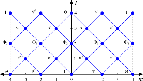
Figure 5: Brattelli diagram of the quasi-particles in the $p=3$ state, which corresponds to the $k=4$ Read-Rezayi state described by the $Z_{4}$ parafermion theory, $SU(2)_{4}/U(1)$. The quasiparticles are indexed by the integers $m$ and $l$. $m$, defined modulo $8$ plays a role similar to $n_{\sigma}$ above, and is determined by the quasiparticle charge. $l$ identifies distinct quasiparticle types for a given charge. The fusion outcomes of any quasiparticle with $\sigma^{+}$ can be deduced by moving one step up or down and to the right.

The case of $p=3$ is one of the Read-Rezayi series of non-Abelian states that are based on electron clustering. The Read-Rezayi series is composed of the states $\nu=k/(mk+2)$, where $k$ is an integer that signifies the number of electrons in a cluster and $m$ is an odd integer (similar states may be constructed for bosons, in which case $m$ is even). For $k=4$ the Read-Rezayi series is given by Eq. (102). The quasi-particles found by identifying the $Z_{4}$ parafermion CFT of the Read-Rezayi approach are identical to those found using our approach. Each quasi-particle is a product of a vertex operator in a free boson charged mode and an operator that acts on a neutral mode. The latter are commonly described by the notation $\Phi_{m}^{l}$ in which $l=0,...,4$, the indices $l+m=0\ ({\rm mod}\ 2)$, and the following identifications $\Phi_{m}^{l}\equiv\Phi_{m+8}^{l}\equiv\Phi_{m-4}^{4-l}$. The $Z_{4}$ parafermion fields, which in our notation are $1$, $\Psi^{+},\Theta,\Psi^{-}$ are here $\Phi_{2j}^{0}$, where $j=0,1,2,3$ respectively. The twist operators are identified in the following way $\sigma^{\pm}=\Phi_{\pm 1}^{1}$, and $\tau^{\pm}=\phi_{\pm 1}^{3}$. The two remaining fields are $\Phi_{\lambda=1}=\Phi_{2}^{2}$ and $\Phi_{\lambda=2}=\Phi_{0}^{2}$. The fusion rules of the various quasi-particles are described by the Brattelli diagram (see Fig. 5) and reproduce the fusion rules of the $p=3$ orbifold theory.

VII.2 Concluding remarks

In this paper we have introduced a coupled wire model for the $Z_{4}$ orbifold quantum Hall states, based on a theory of clustering of electrons into charge $4e$ bosons. On a single wire we employ a mapping to the critical point of the four-state clock model, which exhibits a line of critical points described by the orbifold CFT. Coupling the wires together to form gapped quantum Hall states leads to a sequence of quantum Hall states with an Abelian charge sector coupled to a neutral sector described by the orbifold CFT at a set of discrete radii parametrized by the odd integer $p$. For each odd integer $p$ we identify a solvable theory in which the interactions are tuned to make the electron operators on each wire purely chiral, so that nearest neighbor tunneling, when relevant, necessarily opens a gap.

As discussed in the previous section, $p=1$ is equivalent to an Abelian state, while $p=3$ is equivalent to the $Z_{4}$ parafermion Read-Rezayi state. Larger odd values of $p$ define a set of quantum Hall states that retain the $Z_{4}$ character, but have additional quasiparticle types $\Phi_{\lambda}$. This sequence of orbifold states characterized by the odd integer $p$ has a structure reminiscent of the Laughlin sequence at $\nu=1/m$ for odd integer $m$, which has a similar quasiparticle structure. The difference is that the orbifold states feature the additional twist operators, which lead to a richer non-Abelian structure.

In this paper we have focused exclusively on the orbifold states defined for odd integers $p$. When $p$ is even, our construction breaks down because when $l=2m-p$ is even the electron operator $\psi_{ml}$ in Eq. 56 necessarily involves the twist operators $\sigma_{R}\sigma_{L}$. Since the twist operators retain their identity independent of the orbifold radius, it is not possible to add a forward scattering interaction that modifies the orbifold radius and makes $\psi_{ml}$ a purely chiral operator. Thus, though it is possible for even $p$ to write an electron tunneling term that involves the twist operators, we are not able to find a solvable point with an energy gap. It seems unlikely that such a Hamiltonian would lead to a gapped quantum Hall state.

This leads to interesting questions for further inquiry. One question is what is the nature of the ground state of a clustered coupled wire model with even $p$, when the electron tunneling operator involves the twist operators. If it is not a gapped quantum Hall state, then perhaps it is an interesting gapless state.

Secondly, one can ask whether quantum Hall states characterized by orbifold conformal field theories with even $p$ are possible. The answer to this is certainly yes. As noted in Ref. Dijkgraaf et al., 1989, the orbifold theory is a well defined rational CFT when $p$ is even. This led Barkeshli and WenBarkeshli and Wen (2011) to propose even $p$ orbifold states. However, the fusion rules for even $p$ have a different form than for odd $p$, and have a $Z_{2}\times Z_{2}$ structure, rather than a $Z_{4}$ structure. It therefore seems likely that the physics of the even $p$ orbifold states is not based on clustering of charge $4e$ bosons, but rather involves pairs of charge $2e$ bosons. Analysis of these states will be left for future work.

A further direction is to ask whether the insights gained from the orbifold theory can be applied to clustered states with $k\neq 4$. One interesting approach is the $\epsilon$ expansion in Ref. Sagi et al., 2017, which identified parafermion critical points in an expansion about $k=4+\epsilon$.

Overall, our work demonstrates the power of the coupled wire approach as a tool to generate gapped quantum Hall states and study their topological properties. This tool complements methods employing tools such as analytic single particle wave functions, Jack Polynomials and the thin torus limit Hansson et al. (2017).

Appendix A Relevant Electron Tunneling Operators

In Section V.2 we observed that the electron operators $\tilde{\psi}_{ml}^{\dagger}$ defined in (93) have dimension $\Delta=\Delta_{\rho}+\Delta_{\sigma}$ with $\Delta_{\rho}=|l|/4$ and $\Delta_{\sigma}=p/4$. Without interactions, the electron tunneling term will be irrelevant when $2\Delta>2$. By introducing a local interaction term (88) proportional to $\partial_{x}\bar{\phi}_{i,\rho,R}\partial_{x}\bar{\phi}_{i+1,\rho,L}$ we argued that $\Delta_{\rho}$ can be made arbitrarily small. However, the corresponding operator in the neutral sector, $\partial_{x}\bar{\phi}_{i,\sigma,R}\partial_{x}\bar{\phi}_{i+1,\sigma,L}$, which has the form (124), is not a local operator. This raises the question of whether the tunneling operator can be relevant when $p>3$.

Here we show that there is indeed a local operator that will reduce $\Delta_{\sigma}$, so that $2\Delta<2$, but that operator necessarily also involves the charge sector. Consider the charge $2e$ operator introduced in (115), which is derived from $(\tilde{\psi}_{ml}^{\dagger})^{2}$. In the bosonized representation this has the form

$$\psi_{2e,R}\sim e^{i\pi N_{\sigma}}e^{i4l\bar{\phi}_{\rho R}}\partial_{x}\bar{\phi}_{\sigma R}.$$ (187)

This motivates us to introduce a charge $2e$ tunneling term of the form

$${\cal H}_{{\rm int},i+1/2}^{\prime}=\lambda\cos 4l\bar{\theta}_{i+1/2,\rho}\partial_{x}\bar{\phi}_{i,\sigma R}\bar{\phi}_{i+1,\sigma L}.$$ (188)

When $t_{4}$ is relevant and flows to strong coupling, then $\bar{\theta}_{i+1/2,\rho}$ is pinned at $\pi Q/4l$, where $Q$ is an integer. This leads to an effective interaction in the spin sector of the form

$${\cal H}_{{\rm int},i+1/2}^{\prime}=\lambda(-1)^{Q}\partial_{x}\bar{\phi}_{i,\sigma R}\bar{\phi}_{i+1,\sigma L}.$$ (189)

For fixed $Q$, this leads to a modification of the dimension $\Delta_{\sigma}$. Note that the sign of the interaction depends on $Q$. This reflects the fact that when $Q\rightarrow Q+1$, the spin sector, $\cos(p\bar{\theta}_{\sigma})$ and $\cos(p\bar{\varphi}_{\sigma})$ are interchanged in (110). Changing the sign of the interaction takes $g_{\sigma}\rightarrow 1/g_{\sigma}$, which interchanges the dimensions of $\cos(p\bar{\theta}_{\sigma})$ and $\cos(p\bar{\varphi}_{\sigma})$.

References

- Kane et al. (2002) C. L. Kane, R. Mukhopadhyay, and T. C. Lubensky, Phys. Rev. Lett. 88, 036401 (2002).
- Teo and Kane (2014) J. C. Y. Teo and C. L. Kane, Phys. Rev. B 89, 085101 (2014).
- Neupert et al. (2014) T. Neupert, C. Chamon, C. Mudry, and R. Thomale, Phys. Rev. B 90, 205101 (2014).
- Klinovaja and Tserkovnyak (2014) J. Klinovaja and Y. Tserkovnyak, Phys. Rev. B 90, 115426 (2014).
- Sagi and Oreg (2014) E. Sagi and Y. Oreg, Phys. Rev. B 90, 201102 (2014).
- Santos et al. (2015) R. A. Santos, C.-W. Huang, Y. Gefen, and D. B. Gutman, Phys. Rev. B 91, 205141 (2015).
- Meng et al. (2015) T. Meng, T. Neupert, M. Greiter, and R. Thomale, Phys. Rev. B 91, 241106 (2015).
- Sagi and Oreg (2015) E. Sagi and Y. Oreg, Phys. Rev. B 92, 195137 (2015).
- Huang et al. (2016) P.-H. Huang, J.-H. Chen, P. R. S. Gomes, T. Neupert, C. Chamon, and C. Mudry, Phys. Rev. B 93, 205123 (2016).
- Iadecola et al. (2016) T. Iadecola, T. Neupert, C. Chamon, and C. Mudry, Phys. Rev. B 93, 195136 (2016).
- Mross et al. (2015) D. F. Mross, A. Essin, and J. Alicea, Phys. Rev. X 5, 011011 (2015).
- Mross et al. (2016) D. F. Mross, A. Essin, J. Alicea, and A. Stern, Phys. Rev. Lett. 116, 036803 (2016).
- Klinovaja et al. (2016) J. Klinovaja, P. Stano, and D. Loss, Phys. Rev. Lett. 116, 176401 (2016).
- Fuji and Lecheminant (2017) Y. Fuji and P. Lecheminant, Phys. Rev. B 95, 125130 (2017).
- Haldane (1981a) F. D. M. Haldane, Journal of Physics C: Solid State Physics 14, 2585 (1981a).
- Haldane (1981b) F. D. M. Haldane, Phys. Rev. Lett. 47, 1840 (1981b).
- Laughlin (1983) R. B. Laughlin, Phys. Rev. Lett. 50, 1395 (1983).
- Moore and Read (1991) G. Moore and N. Read, Nuclear Physics B 360, 362 (1991).
- Read and Rezayi (1999) N. Read and E. Rezayi, Phys. Rev. B 59, 8084 (1999).
- Kane et al. (2017) C. L. Kane, A. Stern, and B. I. Halperin, Phys. Rev. X 7, 031009 (2017).
- Read and Green (2000) N. Read and D. Green, Phys. Rev. B 61, 10267 (2000).
- Di Francesco et al. (1997) P. Di Francesco, P. Mathieu, and D. Sénéchal, Conformal field theory, Graduate texts in contemporary physics (Springer, New York, NY, 1997).
- Ginsparg (1988a) P. Ginsparg, in Fields, Strings and Critical Phenomena, (Les Houches, Session XLIX), edited by E. Brézin and J. Zinn-Justin (1988).
- Ginsparg (1988b) P. Ginsparg, Nuclear Physics B 295, 153 (1988b).
- Note (1) Here we use the convention of Ref. \rev@citealpginsparg1988 for the normalization of and .
- Dijkgraaf et al. (1989) R. Dijkgraaf, C. Vafa, E. Verlinde, and H. Verlinde, Comm. Math. Phys. 123, 485 (1989).
- Barkeshli and Wen (2011) M. Barkeshli and X.-G. Wen, Phys. Rev. B 84, 115121 (2011).
- Lecheminant et al. (2002) P. Lecheminant, A. O. Gogolin, and A. A. Nersesyan, Nuclear Physics B 639, 502 (2002).
- Fradkin and Kadanoff (1980) E. Fradkin and L. P. Kadanoff, Nuclear Physics B 170, 1 (1980).
- Zhang and Kane (2014) F. Zhang and C. L. Kane, Phys. Rev. Lett. 113, 036401 (2014).
- Kane and Zhang (2015) C. L. Kane and F. Zhang, Physica Scripta 2015, 014011 (2015).
- Meidan et al. (2017) D. Meidan, E. Berg, and A. Stern, Phys. Rev. B 95, 205104 (2017).
- Lindner et al. (2012) N. H. Lindner, E. Berg, G. Refael, and A. Stern, Phys. Rev. X 2, 041002 (2012).
- J Clarke et al. (2013) D. J Clarke, J. Alicea, and K. Shtengel, Nature communications 4, 1348 (2013).
- Vaezi (2014) A. Vaezi, Phys. Rev. X 4, 031009 (2014).
- Cheng (2012) M. Cheng, Phys. Rev. B 86, 195126 (2012).
- Mong et al. (2014) R. S. K. Mong, D. J. Clarke, J. Alicea, N. H. Lindner, P. Fendley, C. Nayak, Y. Oreg, A. Stern, E. Berg, K. Shtengel, and M. P. A. Fisher, Phys. Rev. X 4, 011036 (2014).
- Wen (2004) X. Wen, Quantum Field Theory of Many-Body Systems: From the Origin of Sound to an Origin of Light and Electrons, Oxford Graduate Texts (OUP Oxford, 2004).
- Bais and Slingerland (2009) F. A. Bais and J. K. Slingerland, Phys. Rev. B 79, 045316 (2009).
- Kitaev (2006) A. Kitaev, Annals of Physics 321, 2 (2006).
- Sagi et al. (2017) E. Sagi, A. Haim, E. Berg, F. von Oppen, and Y. Oreg, Phys. Rev. B 96, 235144 (2017).
- Hansson et al. (2017) T. H. Hansson, M. Hermanns, S. H. Simon, and S. F. Viefers, Rev. Mod. Phys. 89, 025005 (2017).