Context-aware Data Aggregation with Localized Information Privacy

Bo Jiang, Student Member, IEEE, Ming Li, Senior Member, IEEE and Ravi Tandon, Senior Member, IEEE This paper is an extension of our previous work in IEEE CNS2018[1]. B. Jiang M. Li and R. Tandon are with the Department of Electrical and Computer Engineering, University of Arizona, Tucson, AZ, 85742 USA e-mail: {bjiang, lim, tandonr}@email.arizona.edu
Abstract

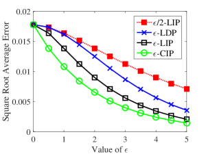
In this paper, localized information privacy (LIP) is proposed, as a new privacy definition, which allows statistical aggregation while protecting users’ privacy without relying on a trusted third party. The notion of context-awareness is incorporated in LIP by the introduction of priors, which enables the design of privacy-preserving data aggregation with knowledge of priors. We show that LIP relaxes the Localized Differential Privacy (LDP) notion by explicitly modeling the adversary’s knowledge. However, it is stricter than 2ϵ2italic-ϵ2\epsilon-LDP and ϵitalic-ϵ\epsilon-mutual information privacy. The incorporation of local priors allows LIP to achieve higher utility compared to other approaches. For four different applications in privacy-preserving data aggregation, including survey, summation, weighted summation and histogram, we present an optimization framework, with the goal of minimizing the mean square error while satisfying the LIP privacy constraints. Utility-privacy tradeoffs are obtained under each model in closed-form, we then theoretically compare with the centralized information privacy and LDP. At last, we validate our analysis by simulations using both synthetic and real-world data. Results show that our LIP mechanism provides better utility-privacy tradeoffs than LDP and when the prior is not uniformly distributed, the advantage of LIP is even more significant.

Index Terms:
privacy-preserving data aggregation, differential privacy, information-theoretic privacy

I Introduction

Privacy issues are crucial in this big data era, as users’ data are collected both intentionally or unintentionally by a large number of private or public organizations. Most of the collected data are used for ensuring high quality of service, but may also put one’s sensitive information at potential risk. For instance, when someone is rating a movie, his/her preferences may be leaked; when someone is searching for a parking spot nearby using a smartphone, his/her real location is uploaded and may be prone to leakage. To mitigate such privacy leakage, it is desirable to design privacy-preserving mechanisms that provide strong privacy guarantees without affecting data utility.

Traditional privacy notions such as k𝑘k-anonymity [2] do not provide rigorous privacy guarantee and are prone to various attacks. On the other hand, Differential Privacy (DP)  [3, 4] has become the defacto𝑑𝑒𝑓𝑎𝑐𝑡𝑜defacto standard for ensuring data privacy in the database community [5]. The definition of DP assures each user’s data has minimal influence on the output of certain types of queries on a database. In the classical DP setting, it is assumed that there is a trusted server which perturbs users’ data while answering queries. However, more often then not, organization collecting users’ data may not be trustworthy and the database storage system may not be secure [6].

Recently, localized privacy protection mechanisms have gained attention as this setting allows local data aggregation while protecting each user’s data without relying on a trusted third party [7]. In localized privacy-preserving data release, each user perturbs his or her data before uploading it; organizations that want to take advantage of users’ data then aggregate with collected users’ published results. Earliest such mechanism is randomized response[8], which randomly perturbs each user’s data. However, the original randomized response does not have formal privacy guarantees. Later, Localized Differential Privacy (LDP) was proposed as a local variant of DP that quantifies the privacy leakage in the local setting[9]. Many schemes were proposed under the notion of LDP. For example, [10, 11, 12], and Google’s RAPPOR [13]. LDP based data aggregation mechanisms have already been deployed in the real-world. For example, in June 2016, Apple announced that it would deploy LDP-based mechanisms to collect user’s typing data [14]. However, Tang et al. show that although each user’s perturbation mechanism satisfies LDP, the privacy budget is too large (ϵ=43italic-ϵ43\epsilon=43)111The parameters, ϵ0italic-ϵ0\epsilon\geq{0}, measures the privacy level. A smaller ϵitalic-ϵ\epsilon corresponds to a higher privacy level. to provide any useful privacy protection. Wang et al. provide a variety of LDP protocols for frequency estimation [15] and compare their performance with Google’s RAPPOR. However, for a given reasonable privacy budget, these protocols provide limited utility. Intuitively, compared with the centralized DP model, it is more challenging to achieve a good utility-privacy tradeoff under the LDP model. The main reasons are two-fold: (1) LDP requires introducing noise at a significantly higher level than what is required in the centralized model. That is, a lower bound of noise magnitude of Ωϵ(N)subscriptΩitalic-ϵ𝑁\Omega_{\epsilon}(\sqrt{N}) is required for LDP, where N𝑁N is the number of users. In contrast, only Oϵ(1)subscript𝑂italic-ϵ1O_{\epsilon}(1) is required for centralized DP [16]. (2) LDP does not assume a neighborhood constraint on users’ data as inputs, thus when the domain of data is very large, LDP leads to a significantly reduced utility [17].

In general, both localized and centralized DP provide strong context-free theoretical guarantees against worst-case adversaries [18]. Context-free means that there is no knowledge of users’ data (either instantaneous or statistical). On the other hand, context-aware privacy notions such as ones where statistical knowledge is available are favorable, as the utility can be increased by explicitly modeling the adversary’s knowledge. Information-theoretic privacy notions [19][20] that incorporate statistical (prior) knowledge fall into this category, which use mutual information (MI) to measure the information leaked about the original database in the released data [21, 22, 23]. Compared with context-free privacy notions, context-aware privacy notions, especially prior-aware notions achieve a better utility-privacy tradeoff [18].

We next discuss a simple illustrative example to motivate the need and advantages of context-aware privacy notions.

Example 1.

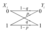
Consider taking a survey over N=100𝑁100N=100 individuals, where each person is independently asked whether he/she has been infected by some kind of disease. It is known based on clinical studies that this disease infects 1 out of 10 people on average. Each individual holds a local true answer Xisubscript𝑋𝑖X_{i}, where i𝑖i is the individual’s index and Xi=1subscript𝑋𝑖1X_{i}=1 if his/her answer is yes, Xi=0subscript𝑋𝑖0X_{i}=0 if the answer is no. For privacy consideration, each individual perturbs his/her data by a randomized response mechanism (shown in Fig. 1) before publishing it. The goal is to estimate the aggregate i=1NXisuperscriptsubscript𝑖1𝑁subscript𝑋𝑖\sum_{i=1}^{N}X_{i} based on Yi,i=1,,Nformulae-sequencesubscript𝑌𝑖𝑖1𝑁Y_{i},i=1,...,N.

Refer to caption
Figure 1: Randomized response mechanism for each individual.

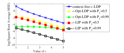
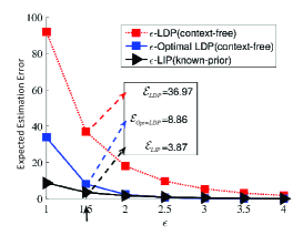
We first assume that the perturbation mechanism satisfies the context-free ϵitalic-ϵ\epsilon-LDP for a given privacy budget ϵitalic-ϵ\epsilon. By the definition of LDP, for each user: max{p1q,q1p,1qp,1pq}ϵ𝑝1𝑞𝑞1𝑝1𝑞𝑝1𝑝𝑞italic-ϵ\max\{\frac{p}{1-q},\frac{q}{1-p},\frac{1-q}{p},\frac{1-p}{q}\}\leq{\epsilon}. In [15], each user’s input Xisubscript𝑋𝑖X_{i} is treated as a fixed instance and a pair of valid solution for (p,q𝑝𝑞p,q) is p=q=1eϵ+1𝑝𝑞1superscript𝑒italic-ϵ1p=q=\frac{1}{e^{\epsilon}+1}. Using the unbiased estimator adopted in [15], the expected error of the aggregate is LDP=Np(1p)(pq)2=100eϵ(eϵ+1)2subscript𝐿𝐷𝑃𝑁𝑝1𝑝superscript𝑝𝑞2100superscript𝑒italic-ϵsuperscriptsuperscript𝑒italic-ϵ12\mathcal{E}_{LDP}=\frac{Np(1-p)}{(p-q)^{2}}=\frac{100e^{\epsilon}}{(e^{\epsilon}+1)^{2}}. The authors then derived an optimal solution for (p,q𝑝𝑞p,q) by minimizing this error while subject to the privacy constraints. Their optimal values of p𝑝p and q𝑞q are different, where q=1eϵ/2superscript𝑞1superscript𝑒italic-ϵ2q^{*}=1-e^{\epsilon}/2 and p=0.5superscript𝑝0.5p^{*}=0.5, resulting in an expected estimation error of OptLDP=25(0.5eϵ/2)2subscript𝑂𝑝𝑡𝐿𝐷𝑃25superscript0.5superscript𝑒italic-ϵ22\mathcal{E}_{Opt-LDP}=\frac{25}{(0.5-e^{\epsilon}/2)^{2}} in our example, which is smaller than LDPsubscript𝐿𝐷𝑃\mathcal{E}_{LDP} (as shown in Fig. 2). This approach increases utility by implicitly using prior knowledge, as it is based on the fact that the answers of a majority of users are zeros (qsuperscript𝑞q^{*} is smaller than psuperscript𝑝p^{*}). Unfortunately, the assumption that Xisubscript𝑋𝑖X_{i}, i=1,2,,N𝑖12𝑁i=1,2,...,N are instances rather than random variables prohibits introducing prior in a principled manner. In addition, the definition of LDP is independent of the priors, which is unable to adjust the perturbation parameters based on different priors. To explicitly introduce prior knowledge, a new privacy definition is needed.
Refer to caption
Figure 2: Comparison among the expected estimation error of different approaches in Example 1: considering prior in the perturbation mechanism significantly reduces the error.

Assuming that each Xisubscript𝑋𝑖X_{i} is a random variable with priors P1=Pr(Xi=1)subscript𝑃1𝑃𝑟subscript𝑋𝑖1P_{1}=Pr({X_{i}=1}) and P0=Pr(Xi=0)subscript𝑃0𝑃𝑟subscript𝑋𝑖0P_{0}=Pr({X_{i}=0}), we propose a context-aware LIP notion which imposes a bound on the ratio between the prior and posterior. In this example, we have: ϵ{Pr(Yi=0)1q,Pr(Yi=0)q,Pr(Yi=1)1p,Pr(Yi=1)p}ϵitalic-ϵ𝑃𝑟subscript𝑌𝑖01𝑞𝑃𝑟subscript𝑌𝑖0𝑞𝑃𝑟subscript𝑌𝑖11𝑝𝑃𝑟subscript𝑌𝑖1𝑝italic-ϵ-\epsilon\leq{\{\frac{Pr(Y_{i}=0)}{1-q},\frac{Pr(Y_{i}=0)}{q},\frac{Pr(Y_{i}=1)}{1-p},\frac{Pr(Y_{i}=1)}{p}}\}\leq{\epsilon}. This notion guarantees that taking observations on the published data provides limited additional information of the real data. Restricted by this privacy notion, the optimal psuperscript𝑝p^{*} and qsuperscript𝑞q^{*} which minimize the mean square error (MSE) can be derived as: q=P1/eϵsuperscript𝑞subscript𝑃1superscript𝑒italic-ϵq^{*}=P_{1}/e^{\epsilon} and p=P0/eϵsuperscript𝑝subscript𝑃0superscript𝑒italic-ϵp^{*}=P_{0}/e^{\epsilon}. Intuitively, it reduces MSE by carefully adjusting p𝑝p and q𝑞q to different priors. By this perturbation mechanism, the resulting error is LIP=10eϵ10.64subscript𝐿𝐼𝑃10superscript𝑒italic-ϵ10.64\mathcal{E}_{LIP}=\frac{10e^{\epsilon}-1}{0.64} which is significantly smaller than LDPsubscript𝐿𝐷𝑃\mathcal{E}_{LDP} (as shown in Fig. 2).

As we discussed above, introducing priors can provide higher utility. However, this comes at the overhead of estimating or learning prior knowledge. This can be obtained in two ways: (1) Sometimes, each individual user’s local prior is available (e.g., can be obtained by training based on historical published data) [24, 25]. For instance, when Google wants to survey multiple users’ current locations to construct a traffic heat-map, it is possible that it already possesses past reported (unperturbed) locations of each user. (2) However, local-prior is relatively strong knowledge on users’ data that may not always be attainable, and one may only be able to learn a global prior (assuming that users’ data are identically distributed). For example, when taking a periodic survey, aggregated results in the recent past can be used as the global prior. Another example is when estimating the frequency of a rare disease, one can leverage the results of past clinical research to obtain a global prior [26].

The main contributions of this paper are three-fold:

(1) We propose a new notion of Localized Information Privacy (LIP) for the local data release setting (without a trusted third party), which relaxes the notion of LDP by introducing priors to increase data utility. We formally show that, ϵitalic-ϵ\epsilon-LIP implies ϵitalic-ϵ\epsilon-Mutual Information Privacy (MIP), and ϵitalic-ϵ\epsilon-LIP is sandwiched between ϵitalic-ϵ\epsilon-LDP and 2ϵitalic-ϵ\epsilon-LDP.

(2) We apply the LIP notion to privacy-preserving data aggregation. Focusing on four applications including: survey, (weighted) summation and histogram, we present a utility-privacy optimization framework with the goal of minimizing the mean squared error while satisfying the LIP constraints. We deploy the randomized response type of perturbation mechanisms. We formulate two perturbation and aggregation models, including: binary-input binary-output (BIBO) model, multiple-input multiple-output (MIMO) model, and derive the corresponding optimal perturbation parameters in closed form and discuss how each application can be realized. We show that one set of the optimal solution can minimize the MSE and the Mean absolute error (MAE) between the raw data and the perturbed data simultaneously. We theoretically demonstrate the advantages of the proposed mechanism and compare with the LDP mechanisms. For comparison, we also study a centralized version of data aggregation under information privacy (CIP), and derive its optimal utility-privacy tradeoff.

(3) We validate our analysis using simulations on both synthetic and real-world datasets (i.e., Karosak, a website-click stream data set, and Gowalla, a location aggregation data set). Both theoretical and simulation results show that optimal perturbation mechanisms under ϵitalic-ϵ\epsilon-LIP always achieve a better utility-privacy tradeoff than those under ϵitalic-ϵ\epsilon-LDP when ϵ>0italic-ϵ0\epsilon>0, especially when the prior is not uniformly distributed. In the MIMO case, We show that when the domain size increases, the advantage of the LIP is enhanced. We show that the advantages of the context-aware LIP are two-fold: on one hand, users are setting the perturbation parameters according to the prior knowledge; on the other hand, the adversary is allowed to build prior-related estimators that can minimize the expected errors. When compared with CIP, it always leads to a better utility-privacy tradeoff than LIP, as the server possesses global information. However, the utility gap is not large.

The remainder of the paper is organized as follows. In Section II, we describe the proposed LIP notion and its relationship with other existing privacy notions. In Section III, we introduce the system model and problem formulation. In Section IV, we derive the utility-privacy tradeoff under the several applications. In Section V, we present the simulation results and compare utility-privacy tradeoffs among different models. In Section VI, we offer concluding remarks and discuss future directions.

II Privacy Definitions

In local privacy-preserving data release, each user uploads its perturbed data directly to an untrusted aggregator. In this section, we first recap two existing privacy notions in localized settings, and then present our new LIP definition.

The traditional LDP definition guarantees that each user’s perturbed data has a similar probability to result in the same output for any two inputs from the data domain 𝔻𝔻\mathbb{D}:

Definition 1.

(ϵitalic-ϵ\epsilon-Localized Differential Privacy (LDP))[27] A mechanism \mathcal{M} which takes input X𝑋X and outputs Y𝑌Y satisfies ϵitalic-ϵ\epsilon-LDP for some ϵ+italic-ϵsuperscript\epsilon\in{\mathbb{R}^{+}}, if x,x𝔻for-all𝑥superscript𝑥𝔻\forall{x,x^{\prime}\in{\mathbb{D}}} and yRange()for-all𝑦𝑅𝑎𝑛𝑔𝑒\forall{y\in{Range(\mathcal{M})}}:

Pr((x)=y)Pr((x)=y)eϵ,𝑃𝑟𝑥𝑦𝑃𝑟superscript𝑥𝑦superscript𝑒italic-ϵ\frac{Pr(\mathcal{M}(x)=y)}{Pr(\mathcal{M}(x^{\prime})=y)}\leq{e^{\epsilon}}, (1)

LDP provides strong context-free privacy guarantee against worst-case adversaries. However, there are many scenarios where some context of X𝑋X is available (e.g., prior distribution). In such situations, introducing context provides relaxed privacy guarantees. One such definition is mutual information privacy, which uses the mutual information between Y𝑌Y, X𝑋X to measure the average information leakage of X𝑋X contained in Y𝑌Y:

Definition 2.

(ϵitalic-ϵ\epsilon-Mutual Information Privacy (MIP))[22] A mechanism \mathcal{M} which takes input X𝑋X and outputs Y𝑌Y, satisfies ϵitalic-ϵ\epsilon-MIP for some ϵ+italic-ϵsuperscript\epsilon\in{\mathbb{R}^{+}}, if the mutual information between X𝑋X and Y𝑌Y satisfies I(X;Y)ϵ𝐼𝑋𝑌italic-ϵI(X;Y)\leq{\epsilon}, where I(X;Y)𝐼𝑋𝑌I(X;Y) is:

x,y𝔻Pr(X=x,Y=y)logPr(X=x,Y=y)Pr(X=x)Pr(Y=y).subscript𝑥𝑦𝔻𝑃𝑟formulae-sequence𝑋𝑥𝑌𝑦𝑃𝑟formulae-sequence𝑋𝑥𝑌𝑦𝑃𝑟𝑋𝑥𝑃𝑟𝑌𝑦\sum_{x,y\in{\mathbb{D}}}Pr(X=x,Y=y)\log\frac{Pr(X=x,Y=y)}{Pr(X=x)Pr(Y=y)}. (2)

Originally, MIP was proposed under the centralized setting where X𝑋X is the database or individual items and Y𝑌Y is a query output. Here we can adapt it to the local setting, where X𝑋X and Y𝑌Y are each individual user’s input and output.

Although MIP is context-aware, it is a relative weak privacy notion since it only bounds the average information leakage. There may exist some (x,y)𝑥𝑦(x,y) pair that makes the ratio between the joint and product of marginal distributions very large (while the joint probability is very small).

In order to limit the information leakage of every pair of realizations of X𝑋X and Y𝑌Y, we consider a bound on the ratio between the prior Pr(X)𝑃𝑟𝑋Pr(X) and posterior Pr(X|Y)𝑃𝑟conditional𝑋𝑌Pr(X|Y), which leads to our proposed localized information privacy notion:

Definition 3.

(ϵitalic-ϵ\epsilon-Localized Information Privacy (LIP)) A mechanism \mathcal{M} which takes input X𝑋X and output Y𝑌Y satisfies ϵitalic-ϵ\epsilon-LIP for some ϵ+italic-ϵsuperscript\epsilon\in{\mathbb{R}^{+}}, if x,y𝔻for-all𝑥𝑦𝔻\forall{x,y\in{\mathbb{D}}}:

eϵPr(X=x)Pr(X=x|Y=y)eϵ.superscript𝑒italic-ϵ𝑃𝑟𝑋𝑥𝑃𝑟𝑋conditional𝑥𝑌𝑦superscript𝑒italic-ϵe^{-\epsilon}\leq{\frac{Pr(X=x)}{Pr(X=x|Y=y)}}\leq{e^{\epsilon}}. (3)

Intuitively, LIP guarantees that having the knowledge of users’ priors, the adversary can’t infer too much additional information about each input x𝑥x by observing each output y𝑦y. Note that, when ϵitalic-ϵ\epsilon is small, this ratio is bounded close to 1. Definition (3) can be viewed as the localized version of information privacy, which focused on a centralized setting [28], and the main differences are in the definitions of input and output. Again, here X𝑋X and Y𝑌Y stand for each user’s input and output variables, respectively.

In the following, We show that LIP is a stronger privacy notion than MIP, since the latter only provides an average privacy guarantee while LIP bounds the leakage on every pair of realizations of X𝑋X and Y𝑌Y.

Proposition 1.

If a mechanism \mathcal{M} satisfies ϵitalic-ϵ\epsilon-LIP, it also satisfies ϵitalic-ϵ\epsilon-MIP.

Proof.

Assume that \mathcal{M} satisfies ϵitalic-ϵ\epsilon-LIP. By Bayes rules, we have that, x,y𝔻for-all𝑥𝑦𝔻\forall x,y\in{\mathbb{D}}:

eϵPr(X=x,Y=y)Pr(X=x)Pr(Y=y)eϵ.superscript𝑒italic-ϵ𝑃𝑟formulae-sequence𝑋𝑥𝑌𝑦𝑃𝑟𝑋𝑥𝑃𝑟𝑌𝑦superscript𝑒italic-ϵe^{-\epsilon}\leq{\frac{Pr(X=x,Y=y)}{Pr(X=x)Pr(Y=y)}}\leq{e^{\epsilon}}. (4)

Substituting (4) into (2), we get:

I(X,Y)ϵx,y𝔻Pr(x,y)=ϵ,𝐼𝑋𝑌italic-ϵsubscript𝑥𝑦𝔻𝑃𝑟𝑥𝑦italic-ϵ\displaystyle I(X,Y)\leq{\epsilon\sum_{x,y\in{\mathbb{D}}}Pr(x,y)}=\epsilon,

where x,y𝔻Pr(x,y)=1subscript𝑥𝑦𝔻𝑃𝑟𝑥𝑦1\sum_{x,y\in{\mathbb{D}}}Pr(x,y)=1.∎

Furthermore, the following theorem shows the relationship between LIP and LDP:

Theorem 1.

If a mechanism \mathcal{M} satisfies ϵitalic-ϵ\epsilon-LIP, then it also satisfies 2ϵ2italic-ϵ2\epsilon-LDP; if a mechanism \mathcal{M} satisfies ϵitalic-ϵ\epsilon-LDP, then it also satisfies ϵitalic-ϵ\epsilon-LIP.

Proof.

To prove the first part, consider a mechanism \mathcal{M} that takes any two inputs X=x𝑋𝑥X=x, X=x𝑋superscript𝑥X=x^{\prime} and outputs the same Y=y𝑌𝑦Y=y.

When \mathcal{M} satisfies ϵitalic-ϵ\epsilon-LIP, using the Bayes rule, Definition (3) is equivalent to:

eϵPr(Y=y)Pr(Y=y|X=x)eϵ.superscript𝑒italic-ϵ𝑃𝑟𝑌𝑦𝑃𝑟𝑌conditional𝑦𝑋𝑥superscript𝑒italic-ϵe^{-\epsilon}\leq{\frac{Pr(Y=y)}{Pr(Y=y|X=x)}}\leq{e^{\epsilon}}. (5)

Since the above also holds for X=x𝑋superscript𝑥X=x^{\prime}, we have:

eϵPr(Y=y)Pr(Y=y|X=x)eϵ.superscript𝑒italic-ϵ𝑃𝑟𝑌𝑦𝑃𝑟𝑌conditional𝑦𝑋superscript𝑥superscript𝑒italic-ϵe^{-\epsilon}\leq{\frac{Pr(Y=y)}{Pr(Y=y|X=x^{\prime})}}\leq{e^{\epsilon}}. (6)

Inequality (5) is equivalent to:

eϵPr(Y=y|X=x)Pr(Y=y)eϵ.superscript𝑒italic-ϵ𝑃𝑟𝑌conditional𝑦𝑋𝑥𝑃𝑟𝑌𝑦superscript𝑒italic-ϵe^{-\epsilon}\leq{\frac{Pr(Y=y|X=x)}{Pr(Y=y)}}\leq{e^{\epsilon}}.

Since both of the metrics in above inequalities are positive, by multiplying these two inequalities, we get:

e2ϵPr(Y=y|X=x)Pr(Y=y|X=x)e2ϵ.superscript𝑒2italic-ϵ𝑃𝑟𝑌conditional𝑦𝑋𝑥𝑃𝑟𝑌conditional𝑦𝑋superscript𝑥superscript𝑒2italic-ϵe^{-2\epsilon}\leq\frac{Pr(Y=y|X=x)}{Pr(Y=y|X=x^{\prime})}\leq{e^{2\epsilon}}.

Since we can switch x𝑥x and xsuperscript𝑥x^{\prime}, it is equivalent to the definition of 2ϵ2italic-ϵ2\epsilon-LDP.

To prove the second part, if \mathcal{M} satisfies ϵitalic-ϵ\epsilon-LDP, we have:

Pr(Y=y|X=x)eϵPr(Y=y|X=x).𝑃𝑟𝑌conditional𝑦𝑋superscript𝑥superscript𝑒italic-ϵ𝑃𝑟𝑌conditional𝑦𝑋𝑥Pr(Y=y|X=x^{\prime})\leq{e^{\epsilon}}Pr(Y=y|X=x).

On the other hand:

Pr(Y=y)=𝑃𝑟𝑌𝑦absent\displaystyle Pr(Y=y)= x𝔻Pr(Y=y|X=x)Pr(X=x)subscriptsuperscript𝑥𝔻𝑃𝑟𝑌conditional𝑦𝑋superscript𝑥𝑃𝑟𝑋superscript𝑥\displaystyle\sum_{x^{\prime}\in{\mathbb{D}}}Pr(Y=y|X=x^{\prime})Pr(X=x^{\prime})
\displaystyle\leq eϵPr(Y=y|X=x)x𝔻Pr(X=x)superscript𝑒italic-ϵ𝑃𝑟𝑌conditional𝑦𝑋𝑥subscriptsuperscript𝑥𝔻𝑃𝑟𝑋superscript𝑥\displaystyle e^{\epsilon}Pr(Y=y|X=x)\sum_{x^{\prime}\in{\mathbb{D}}}Pr(X=x^{\prime})
=\displaystyle= eϵPr(Y=y|X=x),superscript𝑒italic-ϵ𝑃𝑟𝑌conditional𝑦𝑋𝑥\displaystyle e^{\epsilon}Pr(Y=y|X=x),

by switching inputs, we can also get:

Pr(Y=y)eϵPr(Y=y|X=x),𝑃𝑟𝑌𝑦superscript𝑒italic-ϵ𝑃𝑟𝑌conditional𝑦𝑋𝑥Pr(Y=y)\geq{e^{-\epsilon}}Pr(Y=y|X=x),

which means that \mathcal{M} also satisfies ϵitalic-ϵ\epsilon-LIP. ∎

TABLE I: List of symbols
𝔻𝔻\mathbb{D} The universe of input values
X𝑋X Input random variable
P𝑃P User’s prior distribution
Y𝑌Y Output random variable
X¯¯𝑋\bar{X} Set of input data
Y¯¯𝑌\bar{Y} Set of output data
i𝑖i Index User (i{1,2,3,,N}𝑖123𝑁i\in{\{1,2,3,...,N\}})
N𝑁N Total number of users
\mathcal{M} Privacy preserving mechanism
𝐪𝐪\mathbf{q} Set of perturbation parameters
f()𝑓f(\cdot) Aggregation function
X^^𝑋\hat{X} Aggregated data of user
𝐒^^𝐒\hat{\mathbf{S}} Minimized mean square error estimation
ϵitalic-ϵ\epsilon Privacy budget
U𝑈U Utility measurement
\mathcal{E} Mean square error function
𝒯𝒯\mathcal{T} Feasible region of 𝐪𝐪\mathbf{q}

Thus, ϵitalic-ϵ\epsilon-LIP is a more relaxed privacy notion than ϵitalic-ϵ\epsilon-LDP. However, it is stronger than 2ϵ2italic-ϵ2\epsilon-LDP. Intuitively, LIP relaxes LDP because LDP results in the same output y𝑦y for every input x𝑥x, no matter what his/her prior is. On the other hand, for inputs with different priors, LIP perturbs differently. For example, when a user with Pr(X=1)=0.99𝑃𝑟𝑋10.99Pr(X=1)=0.99, if he holds X=1𝑋1X=1, which means his real data is consistent with the prior knowledge. As LIP bounds on the ratio between prior and posterior, it has a large probability to output 111 to make the posterior probability similar to its prior; if he holds X=0𝑋0X=0, which has a small prior to happen, he also has large probability to output 1 to make the posterior probability small.

III Models and Problem Formulation

III-A System and Threat Models
Refer to caption
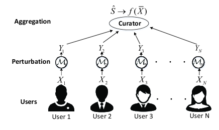
Figure 3: System Model of Privacy-Preserving Data Aggregation.

Consider a data aggregation system with N𝑁N users and a data curator. Each user i𝑖i locally generates private data which is denoted as random variable Xisubscript𝑋𝑖X_{i}, taking value xisubscript𝑥𝑖x_{i} from the domain 𝔻={a1,a2ad}𝔻subscript𝑎1subscript𝑎2subscript𝑎𝑑\mathbb{D}=\{a_{1},a_{2}...a_{d}\} with probability Pki=Pr(Xi=k)subscriptsuperscript𝑃𝑖𝑘𝑃𝑟subscript𝑋𝑖𝑘P^{i}_{k}=Pr(X_{i}=k). We assume that Xisubscript𝑋𝑖X_{i}s are independent from each other. Before publishing his/her data to the curator, each user locally perturbs it by a privacy-preserving mechanism isubscript𝑖\mathcal{M}_{i}. The output is denoted as Yisubscript𝑌𝑖Y_{i} which takes value yisubscript𝑦𝑖y_{i} from 𝔻𝔻\mathbb{D}. The mechanism isubscript𝑖\mathcal{M}_{i} maps each possible input to each possible output with certain probability, the set of them are called perturbation parameters (denoted as 𝐪isuperscript𝐪𝑖\mathbf{q}^{i}). After receiving each user’s perturbed data, the curator computes a statistical function on those data (for example, estimating the frequency of certain input which will be useful for data mining). The system model is depicted in Fig. 3.

The curator is considered as untrusted due to both internal and external threats. On the one hand, users’ private data is profitable and companies can be interested in user tracking or selling their data. On the other hand, data breaches may happen from time to time due to hacking activities. Denote the true aggregated result by f(X¯)𝑓¯𝑋f(\bar{X}), where X¯={X1,X2,,XN}¯𝑋subscript𝑋1subscript𝑋2subscript𝑋𝑁\bar{X}=\{X_{1},X_{2},...,X_{N}\}. The curator (adversary) observes all the users’ perturbed outputs Y¯={Y1,Y2,,YN}¯𝑌subscript𝑌1subscript𝑌2subscript𝑌𝑁\bar{Y}=\{Y_{1},Y_{2},...,Y_{N}\} and tries to obtain an estimate of 𝐒=f(X¯)𝐒𝑓¯𝑋\mathbf{S}=f(\bar{X}). Furthermore, we assume that the adversary possesses knowledge of prior distributions of users’ inputs, and the algorithms/perturbation mechanisms that users adopt to publish their data. The curator aims at performing accurate estimations using all the information above, but is also interested in inferring each user’s real input Xisubscript𝑋𝑖X_{i}.

For different applications of data aggregation, the definition of f()𝑓f(\cdot)s varies. In this paper, four most common applications are considered:

  • Survey: the curator is interested in estimating how many people in the survey possess a private value v𝑣v. Each user’s data can be mapped into a binary bit as: fi(Xi)=𝟙{v=Xi}subscript𝑓𝑖subscript𝑋𝑖subscript1𝑣subscript𝑋𝑖f_{i}(X_{i})=\mathbbm{1}_{\{v={X_{i}}\}}, where 𝟙{a=b}subscript1𝑎𝑏\mathbbm{1}_{\{a=b\}} is an indicator function, which is 1 if a=b𝑎𝑏a=b; 0 if ab𝑎𝑏a\neq{b}. Then the curator just sum up all the collected data to get the answer. Thus 𝐒=f(X¯)=i=1N𝟙{v=Xi}𝐒𝑓¯𝑋subscriptsuperscript𝑁𝑖1subscript1𝑣subscript𝑋𝑖\mathbf{S}=f(\bar{X})=\sum^{N}_{i=1}\mathbbm{1}_{\{v={X_{i}}\}}.

  • Summation: Summation results are usually used to measure an average property of the surveyed individuals. For example, the census bureau wants to survey the average income over a group of people, mathematically, 𝐒=f(X¯)=1Ni=1NXi𝐒𝑓¯𝑋1𝑁subscriptsuperscript𝑁𝑖1subscript𝑋𝑖\mathbf{S}=f(\bar{X})=\frac{1}{N}\sum^{N}_{i=1}{X_{i}}.

  • Weighted summation (linear combination): It’s straightforward to extend the direct summation to a weighted summation (plus an offset) for more general applications. For example, assume that the curator is interested in some particular users more than others, such as employer v.s. employees; adults v.s. children; the professionals v.s. amateurs. Thus, these important users’ data are assigned a larger coefficient than others. The offset can be used as a correction to the raw data. For example, avoiding summation blowing up or controlling data in a particular range. Thus 𝐒=f(X¯)=i=1N(aiXi+bi)𝐒𝑓¯𝑋subscriptsuperscript𝑁𝑖1subscript𝑎𝑖subscript𝑋𝑖subscript𝑏𝑖\mathbf{S}=f(\bar{X})=\sum^{N}_{i=1}{(a_{i}X_{i}+b_{i})}.

  • Histogram: In this application, the curator is interested in estimating how many people possess each of the data category in 𝔻𝔻\mathbbm{D}, or classify people according to their data value. For example, the curator wants to statistically estimate a location frequency matrix with each entry standing for how many people are within a particular location. For this application, 𝐒𝐒\mathbf{S} is a set of ”categorized” data: {S1,S2,,Sd}subscript𝑆1subscript𝑆2subscript𝑆𝑑\{S_{1},S_{2},...,S_{d}\}, such that, k𝔻for-all𝑘𝔻\forall{{k}\in\mathbb{D}}, Sk=i=1N𝟙{Xi=k}subscript𝑆𝑘subscriptsuperscript𝑁𝑖1subscript1subscript𝑋𝑖𝑘S_{k}=\sum^{N}_{i=1}\mathbbm{1}_{\{X_{i}=k\}}.

III-B Privacy and Utility Definitions

The privacy of each user’s input satisfies LIP and is parameterized by the privacy budget (ϵitalic-ϵ\epsilon) in Definition (3). The smaller ϵitalic-ϵ\epsilon is, the higher privacy level the mechanism satisfies. Note that, for simplicity, we consider ϵitalic-ϵ\epsilon to be the same for all the users; however it is straightforward to extend our model and results to different ϵitalic-ϵ\epsilon for different users. Under LIP, the privacy constraints can be formulated as: i{1,2,,N}for-all𝑖12𝑁\forall i\in{\{1,2,...,N\}} and xi,yi𝔻for-allsubscript𝑥𝑖subscript𝑦𝑖𝔻\forall x_{i},y_{i}\in\mathbb{D}, there is

eϵPr(Yi=yi|Xi=xi)Pr(Yi=yi)eϵ.superscript𝑒italic-ϵ𝑃𝑟subscript𝑌𝑖conditionalsubscript𝑦𝑖subscript𝑋𝑖subscript𝑥𝑖𝑃𝑟subscript𝑌𝑖subscript𝑦𝑖superscript𝑒italic-ϵe^{-\epsilon}\leq\frac{Pr(Y_{i}=y_{i}|X_{i}=x_{i})}{Pr(Y_{i}=y_{i})}\leq{e^{\epsilon}}. (7)

Note that, 𝐪i{Pr(Yi=yi|Xi=xi),xi,yi𝔻}superscript𝐪𝑖𝑃𝑟subscript𝑌𝑖conditionalsubscript𝑦𝑖subscript𝑋𝑖subscript𝑥𝑖for-allsubscript𝑥𝑖subscript𝑦𝑖𝔻\mathbf{q}^{i}\triangleq\{Pr(Y_{i}=y_{i}|X_{i}=x_{i}),\forall x_{i},y_{i}\in\mathbb{D}\}. When ϵitalic-ϵ\epsilon is given, the set of inequalities in Eq. (7) constrains 𝐪isuperscript𝐪𝑖\mathbf{q}^{i} to be within a feasible region 𝒯isubscript𝒯𝑖\mathcal{T}_{i}, i1,2,..N\forall{i\in{1,2,..N}}.

The definition of utility depends on the application scenario. For example, in statistical aggregation, estimation accuracy is often measured by absolute error or mean square error [29][30]; in location tracking, it is typically measured by Euclidean distance [24]; in privacy-preserving data publishing, distortion is usually used to measure the utility [22].

Focus on the four applications discussed above, we define utility as the inverse of the Mean Square Error (MSE): U(𝐒,𝐒^)=(𝐒,𝐒^)𝑈𝐒^𝐒𝐒^𝐒U(\mathbf{S},\hat{\mathbf{S}})=-\mathcal{E}(\mathbf{S},\hat{\mathbf{S}}), where (𝐒,𝐒^)=E[(𝐒𝐒^)2]𝐒^𝐒𝐸delimited-[]superscript𝐒^𝐒2\mathcal{E}(\mathbf{S},\hat{\mathbf{S}})=E[(\mathbf{S}-\hat{\mathbf{S}})^{2}], 𝐒^^𝐒\hat{\mathbf{S}} is the estimated 𝐒𝐒\mathbf{S}. Notice that, given Pisuperscript𝑃𝑖P^{i}, (𝐒,𝐒^)𝐒^𝐒\mathcal{E}(\mathbf{S},\hat{\mathbf{S}}) depends only on each user’s perturbation parameters: 𝐪1,,𝐪Nsuperscript𝐪1superscript𝐪𝑁\mathbf{q}^{1},...,\mathbf{q}^{N}, as any estimator 𝐒^^𝐒\hat{\mathbf{S}} will depend on the output Y¯¯𝑌\bar{Y} whose distribution is a function of 𝐪isuperscript𝐪𝑖\mathbf{q}^{i}. Thus, maximizing the utility is equivalent to find the optimal parameters to minimize the MSE.

III-C Problem Formulation

In general, there is a tradeoff between utility and privacy. We can formulate the following optimization problem to find the optimal perturbation mechanism that yields the optimal tradeoff:

min(𝐪1,,𝐪N),superscript𝐪1superscript𝐪𝑁\displaystyle\quad\quad\quad\min\mathcal{E}(\mathbf{q}^{1},...,\mathbf{q}^{N}), (8)
s.t.𝐪i𝒯i,i1,2,..N.\displaystyle s.t.~{}~{}~{}\mathbf{q}^{i}\in{\mathcal{T}_{i}},~{}~{}\forall{i\in{1,2,..N}}.

From [31], it is well known that the optimal estimator that results in the minimized mean square error (MMSE) is 𝐒^=g(Y¯)=E[𝐒|Y¯]^𝐒𝑔¯𝑌𝐸delimited-[]conditional𝐒¯𝑌\hat{\mathbf{S}}=g(\bar{Y})=E[\mathbf{S}|\bar{Y}]. Since E[E[𝐒|Y¯]]=E[𝐒]𝐸delimited-[]𝐸delimited-[]conditional𝐒¯𝑌𝐸delimited-[]𝐒E[E[\mathbf{S}|\bar{Y}]]=E[\mathbf{S}], 𝐒^^𝐒\hat{\mathbf{S}} is an unbiased estimator. Therefore, we use the MMSE estimator in Eq. (8).

Problem Decomposition: Next, we show how the problem defined in Eq. (8) can be decomposed into the local cases.

Since we assume that each user’s input is independent from each other, all the f()𝑓f(\cdot) functions above can be decomposed into local functions of each Xisubscript𝑋𝑖X_{i}: local functions in application 1 and application 4 are indicator functions (or vector); local functions in application 3 is a linear function. Without loss of generality, we denote the local function for user i𝑖i as fisubscript𝑓𝑖f_{i}.

In the local setting, users independently perturb their data, thus each of them results in a MSE in aggregation, which is denoted by i=E[(fi(Xi)E[fi(Xi)|Yi])2]subscript𝑖𝐸delimited-[]superscriptsubscript𝑓𝑖subscript𝑋𝑖𝐸delimited-[]conditionalsubscript𝑓𝑖subscript𝑋𝑖subscript𝑌𝑖2\mathcal{E}_{i}=E[(f_{i}(X_{i})-E[f_{i}(X_{i})|Y_{i}])^{2}] (for the fourth application, denote ik=E[(fik(Xi)E[fik(Xi)|Yi])2]subscriptsuperscript𝑘𝑖𝐸delimited-[]superscriptsubscriptsuperscript𝑓𝑘𝑖subscript𝑋𝑖𝐸delimited-[]conditionalsubscriptsuperscript𝑓𝑘𝑖subscript𝑋𝑖subscript𝑌𝑖2\mathcal{E}^{k}_{i}=E[(f^{k}_{i}(X_{i})-E[f^{k}_{i}(X_{i})|Y_{i}])^{2}]) as the MSE of user i𝑖i when aggregating the k𝑘k-th data, and the overall utility defined in Eq. (8) satisfies decomposition proposition:
Refer to caption
(a) The binary model: different local priors and asymmetric perturbation
Refer to caption
(b) Model with multiple input and multiple output
Refer to caption
(c) Centralized binary information privacy model (trusted server based)
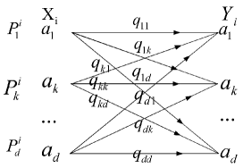
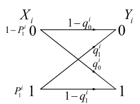
Figure 4: Different models for the perturbation mechanism considered in this paper ((a) and (b) are for the i𝑖i-th user).
Proposition 2.

The global optimization problem defined in Eq. (8) can be decomposed into N𝑁N local optimization problems, under independent user inputs.

min(𝐪i)𝒯i(𝐪1,,𝐪N)=i=1Nmin(𝐪i)𝒯ii(𝐪i).subscriptsuperscript𝐪𝑖subscript𝒯𝑖superscript𝐪1superscript𝐪𝑁superscriptsubscript𝑖1𝑁subscriptsuperscript𝐪𝑖subscript𝒯𝑖subscript𝑖superscript𝐪𝑖\min_{(\mathbf{q}^{i})\in{\mathcal{T}_{i}}}\mathcal{E}(\mathbf{q}^{1},...,\mathbf{q}^{N})=\sum_{i=1}^{N}\min_{(\mathbf{q}^{i})\in{\mathcal{T}_{i}}}\mathcal{E}_{i}(\mathbf{q}^{i}). (9)
Proof.

Observe that, the f()𝑓f(\cdot)s in the four basic applications above can be expressed as a summation over all the fi(Xi)subscript𝑓𝑖subscript𝑋𝑖f_{i}(X_{i})s, as the semantic of aggregation implies a summation operation. thus the summation based MMSE estimator 𝐒^^𝐒\hat{\mathbf{S}} can be expressed as:

E[𝐒|Y¯]=E[f(X¯)|Y¯]=E[{f(X1,X2,,XN)}|Y¯]𝐸delimited-[]conditional𝐒¯𝑌𝐸delimited-[]conditional𝑓¯𝑋¯𝑌𝐸delimited-[]conditional𝑓subscript𝑋1subscript𝑋2subscript𝑋𝑁¯𝑌\displaystyle E[\mathbf{S}|\bar{Y}]=E[f(\bar{X})|\bar{Y}]=E[\{f(X_{1},X_{2},...,X_{N})\}|\bar{Y}] (10)
=(a)𝑎\displaystyle\overset{(a)}{=} E[f1(X1)|Y¯]+E[f2(X2)|Y¯],,+E[fN(XN)|Y¯]}\displaystyle E[f_{1}(X_{1})|\bar{Y}]+E[f_{2}(X_{2})|\bar{Y}],...,+E[f_{N}(X_{N})|\bar{Y}]\}
=(b)𝑏\displaystyle\overset{(b)}{=} i=1N{E[fi(Xi)|Yi]}.subscriptsuperscript𝑁𝑖1𝐸delimited-[]conditionalsubscript𝑓𝑖subscript𝑋𝑖subscript𝑌𝑖\displaystyle\sum^{N}_{i=1}\{E[f_{i}(X_{i})|Y_{i}]\}.

where (a) in Eq. (10) is due to the independence of Xisubscript𝑋𝑖X_{i}s, and (b) is because Xisubscript𝑋𝑖X_{i} is only correlated with Yisubscript𝑌𝑖Y_{i} in the output sequence. Thus (𝐒,𝐒^)𝐒^𝐒\mathcal{E}({\mathbf{S},\hat{\mathbf{S}}}) can be derived as:

(𝐒,𝐒^)=E[(i=1N{fi(Xi)E[fi(Xi)|Yi]})2].𝐒^𝐒𝐸delimited-[]superscriptsubscriptsuperscript𝑁𝑖1subscript𝑓𝑖subscript𝑋𝑖𝐸delimited-[]conditionalsubscript𝑓𝑖subscript𝑋𝑖subscript𝑌𝑖2\mathcal{E}({\mathbf{S},\hat{\mathbf{S}}})=E[(\sum^{N}_{i=1}\{f_{i}(X_{i})-E[f_{i}(X_{i})|Y_{i}]\})^{2}]. (11)

Note that, for the application of histogram, the error forms a error vector that (Sk,Sk^)k=1dsuperscriptsubscriptsubscript𝑆𝑘^subscript𝑆𝑘𝑘1𝑑(S_{k},\hat{S_{k}})_{k=1}^{d}. By the definition of second order norm. the mean square error of this case is:

(Sk,Sk^)k=1d=k=1dE[(i=1N{fik(Xi)E[fik(Xi)|Yi]})2],superscriptsubscriptsubscript𝑆𝑘^subscript𝑆𝑘𝑘1𝑑subscriptsuperscript𝑑𝑘1𝐸delimited-[]superscriptsubscriptsuperscript𝑁𝑖1subscriptsuperscript𝑓𝑘𝑖subscript𝑋𝑖𝐸delimited-[]conditionalsubscriptsuperscript𝑓𝑘𝑖subscript𝑋𝑖subscript𝑌𝑖2\mathcal{E}(S_{k},\hat{S_{k}})_{k=1}^{d}=\sum^{d}_{k=1}E[(\sum^{N}_{i=1}\{f^{k}_{i}(X_{i})-E[f^{k}_{i}(X_{i})|Y_{i}]\})^{2}], (12)

where fik(Xi)=𝟙{Xi=k}subscriptsuperscript𝑓𝑘𝑖subscript𝑋𝑖subscript1subscript𝑋𝑖𝑘f^{k}_{i}(X_{i})=\mathbbm{1}_{\{X_{i}=k\}}.

For the first three applications, we next show that the total MSE can be decompose into the summation of local MSEs. (the proof for histogram is shown in Appendix.D.

(𝐒,𝐒^)=E[(i=1N{fik(Xi)E[fik(Xi)|Yi]})2]𝐒^𝐒𝐸delimited-[]superscriptsubscriptsuperscript𝑁𝑖1subscriptsuperscript𝑓𝑘𝑖subscript𝑋𝑖𝐸delimited-[]conditionalsubscriptsuperscript𝑓𝑘𝑖subscript𝑋𝑖subscript𝑌𝑖2\displaystyle\mathcal{E}({\mathbf{S},\hat{\mathbf{S}}})=E[(\sum^{N}_{i=1}\{f^{k}_{i}(X_{i})-E[f^{k}_{i}(X_{i})|Y_{i}]\})^{2}]
=(i=1NE{fik(Xi)E[fik(Xi)|Yi]})2absentsuperscriptsubscriptsuperscript𝑁𝑖1𝐸subscriptsuperscript𝑓𝑘𝑖subscript𝑋𝑖𝐸delimited-[]conditionalsubscriptsuperscript𝑓𝑘𝑖subscript𝑋𝑖subscript𝑌𝑖2\displaystyle=(\sum^{N}_{i=1}E\{f^{k}_{i}(X_{i})-E[f^{k}_{i}(X_{i})|Y_{i}]\})^{2}
2j=1,ljNE{(fjk(Xi)E[fjk(Xi)|Yj])(flk(Xi)E[flk(Xi)|Yl])}.2subscriptsuperscript𝑁formulae-sequence𝑗1𝑙𝑗𝐸subscriptsuperscript𝑓𝑘𝑗subscript𝑋𝑖𝐸delimited-[]conditionalsubscriptsuperscript𝑓𝑘𝑗subscript𝑋𝑖subscript𝑌𝑗subscriptsuperscript𝑓𝑘𝑙subscript𝑋𝑖𝐸delimited-[]conditionalsubscriptsuperscript𝑓𝑘𝑙subscript𝑋𝑖subscript𝑌𝑙\displaystyle-2\sum^{N}_{j=1,l\neq{j}}E\{(f^{k}_{j}(X_{i})-E[f^{k}_{j}(X_{i})|Y_{j}])(f^{k}_{l}(X_{i})-E[f^{k}_{l}(X_{i})|Y_{l}])\}.

The cross terms equal to 0 because j,l{1,N}for-all𝑗𝑙1𝑁\forall{j,l}\in\{1,N\} and jl𝑗𝑙j\neq{l}:

E{(fjk(Xi)E[fjk(Xi)|Yj])(flk(Xi)E[flk(Xi)|Yl])}]\displaystyle E\{(f^{k}_{j}(X_{i})-E[f^{k}_{j}(X_{i})|Y_{j}])(f^{k}_{l}(X_{i})-E[f^{k}_{l}(X_{i})|Y_{l}])\}] (13)
=\displaystyle= E[(fjk(Xi)E[fjk(Xi)|Yj])]E[(flk(Xi)E[flk(Xi)|Yl])]𝐸delimited-[]subscriptsuperscript𝑓𝑘𝑗subscript𝑋𝑖𝐸delimited-[]conditionalsubscriptsuperscript𝑓𝑘𝑗subscript𝑋𝑖subscript𝑌𝑗𝐸delimited-[]subscriptsuperscript𝑓𝑘𝑙subscript𝑋𝑖𝐸delimited-[]conditionalsubscriptsuperscript𝑓𝑘𝑙subscript𝑋𝑖subscript𝑌𝑙\displaystyle E[(f^{k}_{j}(X_{i})-E[f^{k}_{j}(X_{i})|Y_{j}])]E[(f^{k}_{l}(X_{i})-E[f^{k}_{l}(X_{i})|Y_{l}])]
=\displaystyle= [E(fjk(Xi))E{E[fjk(Xi)|Yj]}][E(flk(Xi))E{E[flk(Xi)|Yl]}].delimited-[]𝐸subscriptsuperscript𝑓𝑘𝑗subscript𝑋𝑖𝐸𝐸delimited-[]conditionalsubscriptsuperscript𝑓𝑘𝑗subscript𝑋𝑖subscript𝑌𝑗delimited-[]𝐸subscriptsuperscript𝑓𝑘𝑙subscript𝑋𝑖𝐸𝐸delimited-[]conditionalsubscriptsuperscript𝑓𝑘𝑙subscript𝑋𝑖subscript𝑌𝑙\displaystyle[E(f^{k}_{j}(X_{i}))-E\{E[f^{k}_{j}(X_{i})|Y_{j}]\}][E(f^{k}_{l}(X_{i}))-E\{E[f^{k}_{l}(X_{i})|Y_{l}]\}].

In (13), E(fjk(Xi))E{E[fjk(Xi)|Yj]}𝐸subscriptsuperscript𝑓𝑘𝑗subscript𝑋𝑖𝐸𝐸delimited-[]conditionalsubscriptsuperscript𝑓𝑘𝑗subscript𝑋𝑖subscript𝑌𝑗E(f^{k}_{j}(X_{i}))-E\{E[f^{k}_{j}(X_{i})|Y_{j}]\} and E(flk(Xi))E{E[flk(Xi)|Yl]}𝐸subscriptsuperscript𝑓𝑘𝑙subscript𝑋𝑖𝐸𝐸delimited-[]conditionalsubscriptsuperscript𝑓𝑘𝑙subscript𝑋𝑖subscript𝑌𝑙E(f^{k}_{l}(X_{i}))-E\{E[f^{k}_{l}(X_{i})|Y_{l}]\} are 0, thus, (𝐒,𝐒^)=i=1Nik(𝐪i)𝐒^𝐒subscriptsuperscript𝑁𝑖1subscriptsuperscript𝑘𝑖superscript𝐪𝑖\mathcal{E}({\mathbf{S},\hat{\mathbf{S}}})=\sum^{N}_{i=1}\mathcal{E}^{k}_{i}(\mathbf{q}^{i})

We next show that the overall optimal solutions (perturbation parameters) satisfy each local privacy constraints:

Assume that for each user, the minimized i(𝐪i)=eisubscript𝑖superscript𝐪𝑖subscript𝑒𝑖\mathcal{E}_{i}(\mathbf{q}^{i})=e_{i} is achieved at 𝐪i𝒯isuperscript𝐪𝑖subscript𝒯𝑖\mathbf{q}^{i*}\in{\mathcal{T}_{i}}, then (𝐪1,,𝐪N)=i=1Neisuperscript𝐪1superscript𝐪𝑁superscriptsubscript𝑖1𝑁subscript𝑒𝑖\mathcal{E}(\mathbf{q}^{1*},...,\mathbf{q}^{N*})=\sum_{i=1}^{N}e_{i}.

If for some userk𝑢𝑠𝑒subscript𝑟𝑘user_{k} who takes parameters 𝐪k𝒯ksuperscript𝐪𝑘subscript𝒯𝑘\mathbf{q}^{k}\in{\mathcal{T}_{k}}, by assumption, we know that k(𝐪k)eksubscript𝑘superscript𝐪𝑘subscript𝑒𝑘\mathcal{E}_{k}(\mathbf{q}^{k})\geq{e_{k}}. Thus

i=1ki(𝐪i)+k(𝐪k)+i=k+1Ni(𝐪i)i=1Nei.superscriptsubscript𝑖1𝑘subscript𝑖superscript𝐪𝑖subscript𝑘superscript𝐪𝑘superscriptsubscript𝑖𝑘1𝑁subscript𝑖superscript𝐪𝑖superscriptsubscript𝑖1𝑁subscript𝑒𝑖\sum_{i=1}^{k}\mathcal{E}_{i}(\mathbf{q}^{i*})+\mathcal{E}_{k}(\mathbf{q}^{k})+\sum_{i=k+1}^{N}\mathcal{E}_{i}(\mathbf{q}^{i*})\geq{\sum_{i=1}^{N}e_{i}}.

That means the minimal value of (𝐪1,,𝐪N)superscript𝐪1superscript𝐪𝑁\mathcal{E}(\mathbf{q}^{1},...,\mathbf{q}^{N}), where 𝐪i𝒯isuperscript𝐪𝑖subscript𝒯𝑖\mathbf{q}^{i}\in{\mathcal{T}_{i}}, i[1,N]for-all𝑖1𝑁\forall{i\in{[1,N]}} can be achieved if for each user, 𝐪i=𝐪isuperscript𝐪𝑖superscript𝐪𝑖\mathbf{q}^{i}=\mathbf{q}^{i*}.

By proposition 2, when the perturbation parameters of each user are optimal, the overall MSE of the mechanism achieves its minimum. In addition, each user can perform its local optimization independent from each other, which well suits the local setting.

Notice that the resulted MSE by a MMSE estimator for each user is i(𝐪i)=E[Var(fi(Xi)|Yi)]subscript𝑖superscript𝐪𝑖𝐸delimited-[]𝑉𝑎𝑟conditionalsubscript𝑓𝑖subscript𝑋𝑖subscript𝑌𝑖\mathcal{E}_{i}(\mathbf{q}^{i})=E[Var(f_{i}(X_{i})|Y_{i})]. By the law of total variance:

E[Var(fi(Xi)|Yi)]𝐸delimited-[]𝑉𝑎𝑟conditionalsubscript𝑓𝑖subscript𝑋𝑖subscript𝑌𝑖\displaystyle E[Var(f_{i}(X_{i})|Y_{i})] (14)
=\displaystyle= Var[fi(Xi)]Var[E(fi(Xi)|Yi)]𝑉𝑎𝑟delimited-[]subscript𝑓𝑖subscript𝑋𝑖𝑉𝑎𝑟delimited-[]𝐸conditionalsubscript𝑓𝑖subscript𝑋𝑖subscript𝑌𝑖\displaystyle Var[f_{i}(X_{i})]-Var[E(f_{i}(X_{i})|Y_{i})]
=\displaystyle= Var[fi(Xi)]Var[fi(X^i)].𝑉𝑎𝑟delimited-[]subscript𝑓𝑖subscript𝑋𝑖𝑉𝑎𝑟delimited-[]subscript𝑓𝑖subscript^𝑋𝑖\displaystyle Var[f_{i}(X_{i})]-Var[f_{i}(\hat{X}_{i})].

In the context-aware setting, Var[fi(Xi)]𝑉𝑎𝑟delimited-[]subscript𝑓𝑖subscript𝑋𝑖Var[f_{i}(X_{i})] is a constant, thus the MSE is a function of the variance of each user’s estimator.

IV Privacy-Utility Trade-off

In this section, we study the privacy-utility tradeoffs by solving the optimization problems defined in Eq. (8). We start by a binary input binary output (BIBO) model where each user has an input/output range of {0,1}01\{0,1\}, which well suits the application of survey. In the BIBO model, we illustrate the way of perturbation by analysis on the optimal solutions. we first assume that fi(Xi)=Xisubscript𝑓𝑖subscript𝑋𝑖subscript𝑋𝑖f_{i}(X_{i})=X_{i} due to settings of the first three applications, we discuss optimal solutions for each of the four applications in section IV-C.

IV-A Utility-Privacy Tradeoff under the Binary Input Binary Output Model

The binary model is widely used for survey: each individual’s data is first mapped to one bit, than randomly perturbed before publishing to the curator.

For a binary input/output model, each user has a binary input range, i.e, 𝔻={0,1}𝔻01\mathbb{D}=\{0,1\} (shown in Fig. 4(a)). As a direct result, the Var(Xi)𝑉𝑎𝑟subscript𝑋𝑖Var(X_{i}) in (14) becomes P1i(1P1i)superscriptsubscript𝑃1𝑖1superscriptsubscript𝑃1𝑖P_{1}^{i}(1-P_{1}^{i}). Denote the perturbation parameters by:

Pr(Yi=1|Xi=0)=q0i,𝑃𝑟subscript𝑌𝑖conditional1subscript𝑋𝑖0subscriptsuperscript𝑞𝑖0\displaystyle Pr(Y_{i}=1|X_{i}=0)=q^{i}_{0}, (15)
Pr(Yi=0|Xi=1)=q1i.𝑃𝑟subscript𝑌𝑖conditional0subscript𝑋𝑖1subscriptsuperscript𝑞𝑖1\displaystyle Pr(Y_{i}=0|X_{i}=1)=q^{i}_{1}.

Next we derive the concrete optimization objective and constraints. By Eq. (10), the MMSE estimator X^isubscript^𝑋𝑖\hat{X}_{i} for user i𝑖i is derived as:

X^i=E[Xi|Yi]=subscript^𝑋𝑖𝐸delimited-[]conditionalsubscript𝑋𝑖subscript𝑌𝑖absent\displaystyle\hat{X}_{i}=E[X_{i}|Y_{i}]= P1i[q1iλ0i(1Yi)+1q1iλ1iYi],subscriptsuperscript𝑃𝑖1delimited-[]subscriptsuperscript𝑞𝑖1subscriptsuperscript𝜆𝑖01subscript𝑌𝑖1subscriptsuperscript𝑞𝑖1subscriptsuperscript𝜆𝑖1subscript𝑌𝑖\displaystyle P^{i}_{1}[\frac{q^{i}_{1}}{\lambda^{i}_{0}}(1-Y_{i})+\frac{1-q^{i}_{1}}{\lambda^{i}_{1}}Y_{i}], (16)

where λ0i=Pr(Yi=0)=(1P1)(1q0i)+P1q1isubscriptsuperscript𝜆𝑖0𝑃𝑟subscript𝑌𝑖01subscript𝑃11subscriptsuperscript𝑞𝑖0subscript𝑃1subscriptsuperscript𝑞𝑖1\lambda^{i}_{0}=Pr(Y_{i}=0)=(1-P_{1})(1-q^{i}_{0})+P_{1}q^{i}_{1} and λ1i=Pr(Yi=1)=(1P1)q0i+P1(1q1i)subscriptsuperscript𝜆𝑖1𝑃𝑟subscript𝑌𝑖11subscript𝑃1subscriptsuperscript𝑞𝑖0subscript𝑃11subscriptsuperscript𝑞𝑖1\lambda^{i}_{1}=Pr(Y_{i}=1)=(1-P_{1})q^{i}_{0}+P_{1}(1-q^{i}_{1}). On the other hand,

Var(X^i)=𝑉𝑎𝑟subscript^𝑋𝑖absent\displaystyle Var(\hat{X}_{i})= Var{P1i[q1iλ0i(1Yi)+1q1iλ1iYi]}𝑉𝑎𝑟subscriptsuperscript𝑃𝑖1delimited-[]subscriptsuperscript𝑞𝑖1subscriptsuperscript𝜆𝑖01subscript𝑌𝑖1subscriptsuperscript𝑞𝑖1subscriptsuperscript𝜆𝑖1subscript𝑌𝑖\displaystyle Var\{P^{i}_{1}[\frac{q^{i}_{1}}{\lambda^{i}_{0}}(1-Y_{i})+\frac{1-q^{i}_{1}}{\lambda^{i}_{1}}Y_{i}]\} (17)
=\displaystyle= P1i(λ0iq1i)2λ0iλ1i.subscriptsuperscript𝑃𝑖1superscriptsubscriptsuperscript𝜆𝑖0superscriptsubscript𝑞1𝑖2subscriptsuperscript𝜆𝑖0subscriptsuperscript𝜆𝑖1\displaystyle P^{i}_{1}\frac{(\lambda^{i}_{0}-q_{1}^{i})^{2}}{\lambda^{i}_{0}\lambda^{i}_{1}}.

Take (17) into (14), the each user’s MSE function i(q0i,q1i)subscript𝑖subscriptsuperscript𝑞𝑖0subscriptsuperscript𝑞𝑖1\mathcal{E}_{i}(q^{i}_{0},q^{i}_{1}) can be derived as

i(q0i,q1i)=P1i(1P1i)[P1i(λ0iq1i)]2λ0iλ1i.subscript𝑖superscriptsubscript𝑞0𝑖superscriptsubscript𝑞1𝑖superscriptsubscript𝑃1𝑖1superscriptsubscript𝑃1𝑖superscriptdelimited-[]subscriptsuperscript𝑃𝑖1subscriptsuperscript𝜆𝑖0superscriptsubscript𝑞1𝑖2subscriptsuperscript𝜆𝑖0subscriptsuperscript𝜆𝑖1\mathcal{E}_{i}(q_{0}^{i},q_{1}^{i})=P_{1}^{i}(1-P_{1}^{i})-\frac{[P^{i}_{1}(\lambda^{i}_{0}-q_{1}^{i})]^{2}}{\lambda^{i}_{0}\lambda^{i}_{1}}.\\ (18)

For the privacy constraints, by Eq. (7), when the perturbation mechanism satisfies ϵitalic-ϵ\epsilon-LIP: we have:

eϵ{F1i,F2i,F3i,F4i}eϵ,i=1,2N.formulae-sequencesuperscript𝑒italic-ϵsubscriptsuperscript𝐹𝑖1subscriptsuperscript𝐹𝑖2subscriptsuperscript𝐹𝑖3subscriptsuperscript𝐹𝑖4superscript𝑒italic-ϵfor-all𝑖12𝑁e^{-\epsilon}\leq{\{F^{i}_{1},F^{i}_{2},F^{i}_{3},F^{i}_{4}\}}\leq{e^{\epsilon}},~{}~{}~{}\forall{i=1,2...N}. (19)

where F1i,F2i,F3i,F4isubscriptsuperscript𝐹𝑖1subscriptsuperscript𝐹𝑖2subscriptsuperscript𝐹𝑖3subscriptsuperscript𝐹𝑖4F^{i}_{1},F^{i}_{2},F^{i}_{3},F^{i}_{4} are directly derived from Definition (3): F1i(q0i,q1i)=λ0iq1isubscriptsuperscript𝐹𝑖1superscriptsubscript𝑞0𝑖superscriptsubscript𝑞1𝑖subscriptsuperscript𝜆𝑖0subscriptsuperscript𝑞𝑖1F^{i}_{1}(q_{0}^{i},q_{1}^{i})=\frac{\lambda^{i}_{0}}{q^{i}_{1}}, F2i(q0i,q1i)=λ1i1q1isubscriptsuperscript𝐹𝑖2superscriptsubscript𝑞0𝑖superscriptsubscript𝑞1𝑖subscriptsuperscript𝜆𝑖11subscriptsuperscript𝑞𝑖1F^{i}_{2}(q_{0}^{i},q_{1}^{i})=\frac{\lambda^{i}_{1}}{1-q^{i}_{1}}, F3i(q0i,q1i)=λ0i1q0isubscriptsuperscript𝐹𝑖3superscriptsubscript𝑞0𝑖superscriptsubscript𝑞1𝑖subscriptsuperscript𝜆𝑖01subscriptsuperscript𝑞𝑖0F^{i}_{3}(q_{0}^{i},q_{1}^{i})=\frac{\lambda^{i}_{0}}{1-q^{i}_{0}}, F4i(q0i,q1i)=λ1iq0isubscriptsuperscript𝐹𝑖4superscriptsubscript𝑞0𝑖superscriptsubscript𝑞1𝑖subscriptsuperscript𝜆𝑖1subscriptsuperscript𝑞𝑖0F^{i}_{4}(q_{0}^{i},q_{1}^{i})=\frac{\lambda^{i}_{1}}{q^{i}_{0}}. Then, the feasible region 𝒯isubscript𝒯𝑖\mathcal{T}_{i} is defined as those (q0i,q1i)superscriptsubscript𝑞0𝑖superscriptsubscript𝑞1𝑖(q_{0}^{i},q_{1}^{i}) pairs satisfying constraints in Eq. (19).

By proposition 2, the optimization problem of Opt-binary-LIP can be reformulated as:

mini(q0i,q1i),subscript𝑖subscriptsuperscript𝑞𝑖0subscriptsuperscript𝑞𝑖1\displaystyle\min{\mathcal{E}_{i}(q^{i}_{0},q^{i}_{1})}, (20)
s.t.formulae-sequence𝑠𝑡\displaystyle s.t. (19),i=1,2N.formulae-sequence(19)for-all𝑖12𝑁\displaystyle\text{ (\ref{eq13})},\forall{i=1,2...N}.

We have the following result:

Theorem 2.

In Opt-binary-LIP, for the i𝑖i-th user, the optimal (q0i,q1i)superscriptsubscript𝑞0𝑖superscriptsubscript𝑞1𝑖(q_{0}^{i},q_{1}^{i}) pairs that minimize i(q0i,q1i)subscript𝑖superscriptsubscript𝑞0𝑖superscriptsubscript𝑞1𝑖\mathcal{E}_{i}(q_{0}^{i},q_{1}^{i}) in problem (LABEL:opt-2) are: either q0i=P1i/eϵsuperscriptsubscript𝑞0𝑖superscriptsubscript𝑃1𝑖superscript𝑒italic-ϵq_{0}^{i*}=P_{1}^{i}/e^{\epsilon} and q1i=(1P1i)/eϵsuperscriptsubscript𝑞1𝑖1superscriptsubscript𝑃1𝑖superscript𝑒italic-ϵq_{1}^{i*}=(1-P_{1}^{i})/e^{\epsilon}, or q0i=1P1i/eϵsuperscriptsubscript𝑞0𝑖1superscriptsubscript𝑃1𝑖superscript𝑒italic-ϵq_{0}^{i*}=1-P_{1}^{i}/e^{\epsilon} and q1i=1(1P1i)/eϵsuperscriptsubscript𝑞1𝑖11superscriptsubscript𝑃1𝑖superscript𝑒italic-ϵq_{1}^{i*}=1-(1-P_{1}^{i})/e^{\epsilon}, for any given ϵ0italic-ϵ0\epsilon\geq 0. The resulting MSE by (q0i,q1isuperscriptsubscript𝑞0𝑖superscriptsubscript𝑞1𝑖q_{0}^{i*},q_{1}^{i*}) is:

biLIP=i=1N{P1i(1P1i)(2eϵe2ϵ)}.subscriptsuperscript𝑏𝑖𝐿𝐼𝑃superscriptsubscript𝑖1𝑁superscriptsubscript𝑃1𝑖1superscriptsubscript𝑃1𝑖2superscript𝑒italic-ϵsuperscript𝑒2italic-ϵ\mathcal{E}^{*}_{bi-LIP}=\sum_{i=1}^{N}\{P_{1}^{i}(1-P_{1}^{i})(2e^{-\epsilon}-e^{-2\epsilon})\}. (21)
Proof.

Here we outline the proof sketch (detailed proofs are shown in Appendix. A.

(1) We show that isubscript𝑖\mathcal{E}_{i} is monotonically increasing with q0isuperscriptsubscript𝑞0𝑖q_{0}^{i} and q1isuperscriptsubscript𝑞1𝑖q_{1}^{i} within the region of {q0i0}{q1i0}{q0i+q1i1}superscriptsubscript𝑞0𝑖0superscriptsubscript𝑞1𝑖0superscriptsubscript𝑞0𝑖superscriptsubscript𝑞1𝑖1\{q_{0}^{i}\geq 0\}\cap\{q_{1}^{i}\geq 0\}\cap\{q_{0}^{i}+q_{1}^{i}\leq{1}\};

(2) We simplify the feasible region 𝒯isubscript𝒯𝑖\mathcal{T}_{i} by showing that both i(q0i,q1i)subscript𝑖superscriptsubscript𝑞0𝑖superscriptsubscript𝑞1𝑖\mathcal{E}_{i}(q_{0}^{i},q_{1}^{i}) and 𝒯isubscript𝒯𝑖\mathcal{T}_{i} are symmetric w.r.t. point (0.5,0.5)0.50.5(0.5,0.5); Then we change 𝒯isubscript𝒯𝑖\mathcal{T}_{i} to the monotonic region in step. (1).

(3) By the monotonicity, showing that the optimal solution is at the boundary of 𝒯isubscript𝒯𝑖\mathcal{T}_{i}, which is a linear function of (q0i,q1i)superscriptsubscript𝑞0𝑖superscriptsubscript𝑞1𝑖(q_{0}^{i},q_{1}^{i}).

(4) The final step is to show that optimal solution is at the intersection of two linear functions in step (3) by testing the monotonicity of i(q0i,q1i)subscript𝑖superscriptsubscript𝑞0𝑖superscriptsubscript𝑞1𝑖\mathcal{E}_{i}(q_{0}^{i},q_{1}^{i}) on the boundary. ∎

Note that, the optimal solution of each user is achieved when F1i(q0i,q1i)=F4i(q0i,q1i)=eϵsubscriptsuperscript𝐹𝑖1superscriptsubscript𝑞0𝑖superscriptsubscript𝑞1𝑖subscriptsuperscript𝐹𝑖4superscriptsubscript𝑞0𝑖superscriptsubscript𝑞1𝑖superscript𝑒italic-ϵF^{i}_{1}(q_{0}^{i},q_{1}^{i})=F^{i}_{4}(q_{0}^{i},q_{1}^{i})=e^{\epsilon} (or F2i(q0i,q1i)=F3i(q0i,q1i)=eϵsubscriptsuperscript𝐹𝑖2superscriptsubscript𝑞0𝑖superscriptsubscript𝑞1𝑖subscriptsuperscript𝐹𝑖3superscriptsubscript𝑞0𝑖superscriptsubscript𝑞1𝑖superscript𝑒italic-ϵF^{i}_{2}(q_{0}^{i},q_{1}^{i})=F^{i}_{3}(q_{0}^{i},q_{1}^{i})=e^{\epsilon}). Intuitively, to increase utility, we need the probability of perturbation as small as possible (when q0i+q1i0.5superscriptsubscript𝑞0𝑖superscriptsubscript𝑞1𝑖0.5q_{0}^{i}+q_{1}^{i}\leq{0.5}), and the smallest perturbation probability is bounded by the privacy constraints. As a result, the optimal solution is at the point where the privacy requirement is just met. The two optimal (q0i,q1i)superscriptsubscript𝑞0𝑖superscriptsubscript𝑞1𝑖(q_{0}^{i*},q_{1}^{i*}) pairs are symmetric w.r.t. (0.5,0.5)0.50.5(0.5,0.5). This is due to the symmetric properties of the binary input/output model. The symmetric properties can also be explained as: if we do not consider privacy, utility is maximized in two ways: the first way is each user publishes his/her data directly; the second way is swapping his/her data from 0 to 1 and 1 to 0 before publishing it.

From q0i=P1i/eϵsuperscriptsubscript𝑞0𝑖superscriptsubscript𝑃1𝑖superscript𝑒italic-ϵq_{0}^{i*}=P_{1}^{i}/e^{\epsilon} and q1i=(1P1i)/eϵsuperscriptsubscript𝑞1𝑖1superscriptsubscript𝑃1𝑖superscript𝑒italic-ϵq_{1}^{i*}=(1-P_{1}^{i})/e^{\epsilon}, we can see that q0isuperscriptsubscript𝑞0𝑖q_{0}^{i*} is proportional to P1isuperscriptsubscript𝑃1𝑖P_{1}^{i}, and q1isuperscriptsubscript𝑞1𝑖q_{1}^{i*} is proportional to 1P1i1superscriptsubscript𝑃1𝑖1-P_{1}^{i}. Intuitively, from the perspective of one user, when his/her true input value xisubscript𝑥𝑖x_{i}’s prior is small, directly revealing xisubscript𝑥𝑖x_{i} will leak too much information about it. In such cases, to satisfy LIP constraints, a large perturbation probability is needed to limit the posterior about xisubscript𝑥𝑖x_{i}. On the contrary, if xisubscript𝑥𝑖x_{i} happens with a large prior, directly releasing xisubscript𝑥𝑖x_{i} will reveal little additional information. Thus a small perturbation probability can be used for xisubscript𝑥𝑖x_{i} in this case.

Minimizing mean absolute error between the raw data and the perturbed data: In many applications, the published data by each user should contain certain information even for the parties with no prior knowledge. For example, the reported locations from smart phones: facilities or companies want to take advantages from the aggregated location data frequencies on one hand, the users are uploading locations for location based service on the other. As a result, although the locally published data are perturbed, it should remain a certain level of accuracy. As a result, We want Yisubscript𝑌𝑖Y_{i} as close to Xisubscript𝑋𝑖X_{i} as possible as long as it still satisfies the privacy constraints. As Pisuperscript𝑃𝑖P^{i} is given, we want the mean absolute error (MAE) between Xisubscript𝑋𝑖X_{i} and Yisubscript𝑌𝑖Y_{i} as small as possible, that is, we also want to minimize:

E[|XiYi|],i{1,2,,N}.𝐸delimited-[]subscript𝑋𝑖subscript𝑌𝑖for-all𝑖12𝑁E[|X_{i}-Y_{i}|],\forall{i\in\{1,2,...,N\}}. (22)

Regarding at the optimal solutions of the binary model, we have the following proposition:

Proposition 3.

The optimal solution that minimize the MSE defined in (18) and the MAE defined in (22) simultaneously is: q0i=P1i/eϵsuperscriptsubscript𝑞0𝑖superscriptsubscript𝑃1𝑖superscript𝑒italic-ϵq_{0}^{i*}=P_{1}^{i}/e^{\epsilon} and q1i=(1P1i)/eϵsuperscriptsubscript𝑞1𝑖1superscriptsubscript𝑃1𝑖superscript𝑒italic-ϵq_{1}^{i*}=(1-P_{1}^{i})/e^{\epsilon}.

Proof.

Notice that there are two set of optimal solutions under the Opt-binary-LIP model.

The MAE defined in (22)italic-(22italic-)\eqref{eqMAE} is

xi=01yi=01|xiyi|Pr(Xi=xi)Pr(Yi=yi|Xi=xi)subscriptsuperscript1subscript𝑥𝑖0subscriptsuperscript1subscript𝑦𝑖0subscript𝑥𝑖subscript𝑦𝑖𝑃𝑟subscript𝑋𝑖subscript𝑥𝑖𝑃𝑟subscript𝑌𝑖conditionalsubscript𝑦𝑖subscript𝑋𝑖subscript𝑥𝑖\displaystyle\sum^{1}_{x_{i}=0}\sum^{1}_{y_{i}=0}|x_{i}-y_{i}|Pr(X_{i}=x_{i})Pr(Y_{i}=y_{i}|X_{i}=x_{i}) (23)
=\displaystyle= P1iq1i+(1P1i)q0i.subscriptsuperscript𝑃𝑖1subscriptsuperscript𝑞𝑖11subscriptsuperscript𝑃𝑖1subscriptsuperscript𝑞𝑖0\displaystyle P^{i}_{1}q^{i}_{1}+(1-P^{i}_{1})q^{i}_{0}.

As P1isubscriptsuperscript𝑃𝑖1P^{i}_{1} is given, minimizing (23) is equivalent to minimize q1isubscriptsuperscript𝑞𝑖1q^{i}_{1} and q0isubscriptsuperscript𝑞𝑖0q^{i}_{0}, which are also restricted by the privacy constraint, thus the optimal solution q0i=P1i/eϵsuperscriptsubscript𝑞0𝑖superscriptsubscript𝑃1𝑖superscript𝑒italic-ϵq_{0}^{i*}=P_{1}^{i}/e^{\epsilon} and q1i=(1P1i)/eϵsuperscriptsubscript𝑞1𝑖1superscriptsubscript𝑃1𝑖superscript𝑒italic-ϵq_{1}^{i*}=(1-P_{1}^{i})/e^{\epsilon} can also minimize the MAE. ∎

From the result of proposition. 3, we can see a trend from the optimal perturbation parameters that minimize the MAE and MSE at the same time, that is when ϵitalic-ϵ\epsilon increase, the raw data is more likely to be directly published. Notice that, with the optimal solutions,

λ0i=subscriptsuperscript𝜆𝑖0absent\displaystyle\lambda^{i}_{0}= P1i(1P1i)eϵ+(1P1i)(1P1ieϵ)=(1P1i),subscriptsuperscript𝑃𝑖11subscriptsuperscript𝑃𝑖1superscript𝑒italic-ϵ1subscriptsuperscript𝑃𝑖11subscriptsuperscript𝑃𝑖1superscript𝑒italic-ϵ1subscriptsuperscript𝑃𝑖1\displaystyle P^{i}_{1}\frac{(1-P^{i}_{1})}{e^{\epsilon}}+(1-P^{i}_{1})(1-\frac{P^{i}_{1}}{e^{\epsilon}})=(1-P^{i}_{1}),
λ1i=subscriptsuperscript𝜆𝑖1absent\displaystyle\lambda^{i}_{1}= P1i(1(1P1i)eϵ)+(1P1i)P1ieϵ=P1i.subscriptsuperscript𝑃𝑖111subscriptsuperscript𝑃𝑖1superscript𝑒italic-ϵ1subscriptsuperscript𝑃𝑖1subscriptsuperscript𝑃𝑖1superscript𝑒italic-ϵsubscriptsuperscript𝑃𝑖1\displaystyle P^{i}_{1}(1-\frac{(1-P^{i}_{1})}{e^{\epsilon}})+(1-P^{i}_{1})\frac{P^{i}_{1}}{e^{\epsilon}}=P^{i}_{1}.

Thus the distribution of each Xisubscript𝑋𝑖X_{i} is identical to Yisubscript𝑌𝑖Y_{i}, this also guarantees that the output Yisubscript𝑌𝑖Y_{i} is very close to Xisubscript𝑋𝑖X_{i}.

Comparison with Optimized LDP: We next compare our optimal LIP-based perturbation mechanism with the optimal LDP-based one. Define the Opt-binary-LDP problem to be the same with Opt-binary-LIP in (LABEL:opt-2), except having different privacy constraints of LDP: {R1i,R2i,R3i,R4i}eϵsuperscriptsubscript𝑅1𝑖superscriptsubscript𝑅2𝑖superscriptsubscript𝑅3𝑖superscriptsubscript𝑅4𝑖superscript𝑒italic-ϵ\{R_{1}^{i},R_{2}^{i},R_{3}^{i},R_{4}^{i}\}\leq{e^{\epsilon}}, where R1i,R2i,R3i,R4isuperscriptsubscript𝑅1𝑖superscriptsubscript𝑅2𝑖superscriptsubscript𝑅3𝑖superscriptsubscript𝑅4𝑖R_{1}^{i},R_{2}^{i},R_{3}^{i},R_{4}^{i} are derived from Definition (1): R1i=1q1iq0isuperscriptsubscript𝑅1𝑖1superscriptsubscript𝑞1𝑖superscriptsubscript𝑞0𝑖R_{1}^{i}=\frac{1-q_{1}^{i}}{q_{0}^{i}}, R2i=q0i1q1isuperscriptsubscript𝑅2𝑖superscriptsubscript𝑞0𝑖1superscriptsubscript𝑞1𝑖R_{2}^{i}=\frac{q_{0}^{i}}{1-q_{1}^{i}}, R3i=q1i1q0isuperscriptsubscript𝑅3𝑖superscriptsubscript𝑞1𝑖1subscriptsuperscript𝑞𝑖0R_{3}^{i}=\frac{q_{1}^{i}}{1-q^{i}_{0}} and R4i=1q0iq1isuperscriptsubscript𝑅4𝑖1superscriptsubscript𝑞0𝑖superscriptsubscript𝑞1𝑖R_{4}^{i}=\frac{1-q_{0}^{i}}{q_{1}^{i}}.

Proposition 4.

In Opt-binary-LDP, for the i𝑖i-th user, the optimal solution for (q0i,q1i)subscriptsuperscript𝑞𝑖0subscriptsuperscript𝑞𝑖1(q^{i}_{0},q^{i}_{1}) is q0i=q1i=1eϵ+1superscriptsubscript𝑞0𝑖superscriptsubscript𝑞1𝑖1superscript𝑒italic-ϵ1q_{0}^{i*}=q_{1}^{i*}=\frac{1}{e^{\epsilon}+1}, which results in a MSE biLDPsubscriptsuperscript𝑏𝑖𝐿𝐷𝑃\mathcal{E}^{*}_{bi-LDP} of:

i=1N{P1i(1P1i)[P1i(1P1i)(1eϵ)]2(1P1i+P1ieϵ)(eϵP1ieϵ+P1i)}.superscriptsubscript𝑖1𝑁superscriptsubscript𝑃1𝑖1superscriptsubscript𝑃1𝑖superscriptdelimited-[]superscriptsubscript𝑃1𝑖1superscriptsubscript𝑃1𝑖1superscript𝑒italic-ϵ21superscriptsubscript𝑃1𝑖superscriptsubscript𝑃1𝑖superscript𝑒italic-ϵsuperscript𝑒italic-ϵsuperscriptsubscript𝑃1𝑖superscript𝑒italic-ϵsuperscriptsubscript𝑃1𝑖\sum_{i=1}^{N}\{P_{1}^{i}(1-P_{1}^{i})-\frac{[P_{1}^{i}(1-P_{1}^{i})(1-e^{\epsilon})]^{2}}{(1-P_{1}^{i}+P_{1}^{i}e^{\epsilon})(e^{\epsilon}-P_{1}^{i}e^{\epsilon}+P_{1}^{i})}\}. (24)

Given any fixed ϵ0italic-ϵ0\epsilon\geq 0, we have biLDPbiLIPsubscriptsuperscript𝑏𝑖𝐿𝐷𝑃subscriptsuperscript𝑏𝑖𝐿𝐼𝑃\mathcal{E}^{*}_{bi-LDP}\geq{\mathcal{E}^{*}_{bi-LIP}}.

Proof.

The proof of the optimal solution is similar to that of Opt-binary-LIP, the only difference is the feasible region in Opt-binary-LIP is flexible for different priors, while the feasible region in Opt-binary-LDP is fixed. The optimal solution also coincides with the one used in [15].

For the second part, it’s easy to check by taking derivative over eϵsuperscript𝑒italic-ϵe^{\epsilon} that biLIPbiLDPsubscriptsuperscript𝑏𝑖𝐿𝐼𝑃subscriptsuperscript𝑏𝑖𝐿𝐷𝑃\mathcal{E}^{*}_{bi-LIP}\leq{\mathcal{E}^{*}_{bi-LDP}}, where biLIP=biLDPsubscriptsuperscript𝑏𝑖𝐿𝐼𝑃subscriptsuperscript𝑏𝑖𝐿𝐷𝑃\mathcal{E}^{*}_{bi-LIP}={\mathcal{E}^{*}_{bi-LDP}} if ϵ=0italic-ϵ0\epsilon=0 or ϵ=italic-ϵ\epsilon=\infty. This means LIP provides increased utility given any ϵitalic-ϵ\epsilon. We then taking derivative of P1isubscriptsuperscript𝑃𝑖1P^{i}_{1} over Δ=biLDPbiLIPΔsuperscriptsubscriptsuperscript𝑏𝑖𝐿𝐷𝑃subscriptsuperscript𝑏𝑖𝐿𝐼𝑃\Delta\mathcal{E}^{*}=\mathcal{E}^{*}_{bi-LDP}-\mathcal{E}^{*}_{bi-LIP}, result shows that ΔP1i=0Δsuperscriptsubscriptsuperscript𝑃𝑖10\frac{\partial\Delta\mathcal{E}^{*}}{\partial{P^{i}_{1}}}=0 when P1i=0.5subscriptsuperscript𝑃𝑖10.5P^{i}_{1}=0.5. As Δ(P1i=0.5)0Δsubscriptsuperscriptsubscriptsuperscript𝑃𝑖10.50\Delta\mathcal{E}^{*}_{(P^{i}_{1}=0.5)}\geq{0}, biLDPbiLIPsubscriptsuperscript𝑏𝑖𝐿𝐷𝑃subscriptsuperscript𝑏𝑖𝐿𝐼𝑃\mathcal{E}^{*}_{bi-LDP}\geq\mathcal{E}^{*}_{bi-LIP} for any P1isubscriptsuperscript𝑃𝑖1P^{i}_{1}. Result also shows that as |P1i0.5|subscriptsuperscript𝑃𝑖10.5|P^{i}_{1}-0.5| grows, ΔΔsuperscript\Delta\mathcal{E}^{*} also increases. ∎

The above result shows that, Opt-binary-LIP always achieves a better utility than Opt-binary-LDP under any ϵitalic-ϵ\epsilon, this is because explicitly considering prior in the privacy definition allows a larger search space for optimal parameters than that in Opt-binary-LDP. We can also learn this result from the aspect of information theory, when |P1i0.5|subscriptsuperscript𝑃𝑖10.5|P^{i}_{1}-0.5| is small, then the H(Xi)𝐻subscript𝑋𝑖H(X_{i}) is large, which means Xisubscript𝑋𝑖X_{i} has the largest amount of uncertainty, thus knowing the prior of Xisubscript𝑋𝑖X_{i} does not help in perturbation; However, when H(Xi)𝐻subscript𝑋𝑖H(X_{i}) is small, prior knowledge of Xisubscript𝑋𝑖X_{i} provides a clearer indication of the real value, thus the context-aware model achieves enhanced advantages.

The binary case is an illustrative example that shows how we derive the optimal solutions, as the problem is equivalent to finding the maximum in a monotonically increasing region, thus the methods with goal to find the station points in the feasible region such as Lagrangian multiplier and KKT conditions are not applicable. On the other hand, thanks to the theorem that the maximum value of the monotocity function can be found at the boundary, the problem can be first regarded as developing the monotocity region and then finding the boundary values of the parameters. Moreover, with the goal to minimize the MAE, we can further restrict the optimal solutions to make the model more practical.

When each user has a same prior and when the perturbation channel is symmetric, these can be considered as special cases of the BIBO model, and details are referred to our conference version in [1].

IV-B Utility-Privacy Tradeoff under MIMO Model

More generally, we study the case in which 𝔻𝔻\mathbb{D} has a large domain, i.e., 𝔻={a1,a2,,ad}𝔻subscript𝑎1subscript𝑎2subscript𝑎𝑑\mathbb{D}=\{a_{1},a_{2},...,a_{d}\} with prior distribution Pr(Xi=am)=Pmi𝑃𝑟subscript𝑋𝑖subscript𝑎𝑚subscriptsuperscript𝑃𝑖𝑚Pr(X_{i}=a_{m})=P^{i}_{m}. This case well suits the application of summation and weighted summation and we denote this model as MIMO model. The optimization of the MIMO model is obviously obscure, as there are d2superscript𝑑2d^{2} parameters that need to optimize for a single user. (shown in 4(b))

Assume that a random-response perturbation mechanism which satisfies ϵitalic-ϵ\epsilon-LIP takes input Xisubscript𝑋𝑖X_{i} and output Yisubscript𝑌𝑖Y_{i} (Yisubscript𝑌𝑖Y_{i} has the same range, we discuss the optimal output range after deriving the main results) with probability Pr(Yi=ak|Xi=am)=qmki𝑃𝑟subscript𝑌𝑖conditionalsubscript𝑎𝑘subscript𝑋𝑖subscript𝑎𝑚subscriptsuperscript𝑞𝑖𝑚𝑘Pr(Y_{i}=a_{k}|X_{i}=a_{m})=q^{i}_{mk}. Denote Pr(Yi=ak)=λki𝑃𝑟subscript𝑌𝑖subscript𝑎𝑘subscriptsuperscript𝜆𝑖𝑘Pr(Y_{i}=a_{k})=\lambda^{i}_{k} . Thus, by (7):

eϵPr(Xi=am)Pr(Xi=am|Yi=ak)eϵ,m,k1,2,,dformulae-sequencesuperscript𝑒italic-ϵ𝑃𝑟subscript𝑋𝑖subscript𝑎𝑚𝑃𝑟subscript𝑋𝑖conditionalsubscript𝑎𝑚subscript𝑌𝑖subscript𝑎𝑘superscript𝑒italic-ϵfor-all𝑚𝑘12𝑑e^{-\epsilon}\leq\frac{Pr(X_{i}=a_{m})}{Pr(X_{i}=a_{m}|Y_{i}=a_{k})}\leq{e^{\epsilon}},\forall{m,k\in{1,2,...,d}} (25)

By Bayes rules, (25) can be transferred to:

eϵλkiqmkieϵ,m,k1,2,,dformulae-sequencesuperscript𝑒italic-ϵsubscriptsuperscript𝜆𝑖𝑘subscriptsuperscript𝑞𝑖𝑚𝑘superscript𝑒italic-ϵfor-all𝑚𝑘12𝑑e^{-\epsilon}\leq\frac{\lambda^{i}_{k}}{q^{i}_{mk}}\leq{e^{\epsilon}},\forall{m,k\in{1,2,...,d}} (26)

In (14), Var[Xi]=m=1dam2Pmi(m=1damPmi)2𝑉𝑎𝑟delimited-[]subscript𝑋𝑖subscriptsuperscript𝑑𝑚1superscriptsubscript𝑎𝑚2subscriptsuperscript𝑃𝑖𝑚superscriptsubscriptsuperscript𝑑𝑚1subscript𝑎𝑚subscriptsuperscript𝑃𝑖𝑚2Var[X_{i}]=\sum^{d}_{m=1}a_{m}^{2}P^{i}_{m}-(\sum^{d}_{m=1}a_{m}P^{i}_{m})^{2}, and

Xi^=^subscript𝑋𝑖absent\displaystyle\hat{X_{i}}= E[Xi|Yi]=m=1dajPr(Xi=am|Yi)𝐸delimited-[]conditionalsubscript𝑋𝑖subscript𝑌𝑖subscriptsuperscript𝑑𝑚1subscript𝑎𝑗𝑃𝑟subscript𝑋𝑖conditionalsubscript𝑎𝑚subscript𝑌𝑖\displaystyle E[X_{i}|Y_{i}]=\sum^{d}_{m=1}a_{j}Pr(X_{i}=a_{m}|Y_{i}) (27)
=\displaystyle= m=1dk=1damPr(Xi=am|Yi=ak)𝟙ki,subscriptsuperscript𝑑𝑚1subscriptsuperscript𝑑𝑘1subscript𝑎𝑚𝑃𝑟subscript𝑋𝑖conditionalsubscript𝑎𝑚subscript𝑌𝑖subscript𝑎𝑘subscriptsuperscript1𝑖𝑘\displaystyle\sum^{d}_{m=1}\sum^{d}_{k=1}a_{m}Pr(X_{i}=a_{m}|Y_{i}=a_{k})\mathbbm{1}^{i}_{k},

where 𝟙kisubscriptsuperscript1𝑖𝑘\mathbbm{1}^{i}_{k} is the indicator function of 𝟙{Yi=ak}isubscriptsuperscript1𝑖subscript𝑌𝑖subscript𝑎𝑘\mathbbm{1}^{i}_{\{Y_{i}=a_{k}\}}, which is 1 if Yi=aksubscript𝑌𝑖subscript𝑎𝑘Y_{i}=a_{k} and 0 if not, thus 𝟙kisubscriptsuperscript1𝑖𝑘\mathbbm{1}^{i}_{k} can be regarded as a binary random variable which has the distribution of: Pr(𝟙ki=1)=λki𝑃𝑟subscriptsuperscript1𝑖𝑘1subscriptsuperscript𝜆𝑖𝑘Pr(\mathbbm{1}^{i}_{k}=1)=\lambda^{i}_{k} and Pr(𝟙ki=0)=1λki𝑃𝑟subscriptsuperscript1𝑖𝑘01subscriptsuperscript𝜆𝑖𝑘Pr(\mathbbm{1}^{i}_{k}=0)=1-\lambda^{i}_{k}, as a result: Var[𝟙ki]=λki(1λki)𝑉𝑎𝑟delimited-[]subscriptsuperscript1𝑖𝑘subscriptsuperscript𝜆𝑖𝑘1subscriptsuperscript𝜆𝑖𝑘Var[\mathbbm{1}^{i}_{k}]=\lambda^{i}_{k}(1-\lambda^{i}_{k}) and Cov[𝟙ki,𝟙li]=λkiλli𝐶𝑜𝑣subscriptsuperscript1𝑖𝑘subscriptsuperscript1𝑖𝑙subscriptsuperscript𝜆𝑖𝑘subscriptsuperscript𝜆𝑖𝑙Cov[\mathbbm{1}^{i}_{k},\mathbbm{1}^{i}_{l}]=-\lambda^{i}_{k}\lambda^{i}_{l}.

Var[Xi^]=m=1dn=1dk=1damanqmkiqnkiVar[𝟙ki]𝑉𝑎𝑟delimited-[]^subscript𝑋𝑖subscriptsuperscript𝑑𝑚1subscriptsuperscript𝑑𝑛1subscriptsuperscript𝑑𝑘1subscript𝑎𝑚subscript𝑎𝑛subscriptsuperscript𝑞𝑖𝑚𝑘subscriptsuperscript𝑞𝑖𝑛𝑘𝑉𝑎𝑟delimited-[]subscriptsuperscript1𝑖𝑘\displaystyle Var[\hat{X_{i}}]=\sum^{d}_{m=1}\sum^{d}_{n=1}\sum^{d}_{k=1}a_{m}a_{n}q^{i}_{mk}q^{i}_{nk}Var[\mathbbm{1}^{i}_{k}] (28)
+\displaystyle+ m=1dn=1dk=1dl=1;lkdamanqmkiqnliCov[𝟙ki,𝟙li]subscriptsuperscript𝑑𝑚1subscriptsuperscript𝑑𝑛1subscriptsuperscript𝑑𝑘1subscriptsuperscript𝑑formulae-sequence𝑙1𝑙𝑘subscript𝑎𝑚subscript𝑎𝑛subscriptsuperscript𝑞𝑖𝑚𝑘subscriptsuperscript𝑞𝑖𝑛𝑙𝐶𝑜𝑣subscriptsuperscript1𝑖𝑘subscriptsuperscript1𝑖𝑙\displaystyle\sum^{d}_{m=1}\sum^{d}_{n=1}\sum^{d}_{k=1}\sum^{d}_{l=1;l\neq{k}}a_{m}a_{n}q^{i}_{mk}q^{i}_{nl}Cov[\mathbbm{1}^{i}_{k},\mathbbm{1}^{i}_{l}]
=\displaystyle= m=1dn=1dk=1damanPmiPniqmki(qnki(1λki)λkil=1;lkdqnli)subscriptsuperscript𝑑𝑚1subscriptsuperscript𝑑𝑛1subscriptsuperscript𝑑𝑘1subscript𝑎𝑚subscript𝑎𝑛subscriptsuperscript𝑃𝑖𝑚subscriptsuperscript𝑃𝑖𝑛subscriptsuperscript𝑞𝑖𝑚𝑘subscriptsuperscript𝑞𝑖𝑛𝑘1subscriptsuperscript𝜆𝑖𝑘subscriptsuperscript𝜆𝑖𝑘subscriptsuperscript𝑑formulae-sequence𝑙1𝑙𝑘subscriptsuperscript𝑞𝑖𝑛𝑙\displaystyle\sum^{d}_{m=1}\sum^{d}_{n=1}\sum^{d}_{k=1}a_{m}a_{n}P^{i}_{m}P^{i}_{n}q^{i}_{mk}(\frac{q^{i}_{nk}(1-\lambda^{i}_{k})}{\lambda^{i}_{k}}-\sum^{d}_{l=1;l\neq{k}}q^{i}_{nl})
=\displaystyle= m=1dn=1dk=1damanPmiPniqmki(qnkiλki1).subscriptsuperscript𝑑𝑚1subscriptsuperscript𝑑𝑛1subscriptsuperscript𝑑𝑘1subscript𝑎𝑚subscript𝑎𝑛subscriptsuperscript𝑃𝑖𝑚subscriptsuperscript𝑃𝑖𝑛subscriptsuperscript𝑞𝑖𝑚𝑘subscriptsuperscript𝑞𝑖𝑛𝑘subscriptsuperscript𝜆𝑖𝑘1\displaystyle\sum^{d}_{m=1}\sum^{d}_{n=1}\sum^{d}_{k=1}a_{m}a_{n}P^{i}_{m}P^{i}_{n}q^{i}_{mk}(\frac{q^{i}_{nk}}{\lambda^{i}_{k}}-1).

Denote 𝐪𝐢superscript𝐪𝐢\mathbf{q^{i}} as the set of {q11i,q12i,,q1di,,qddi}subscriptsuperscript𝑞𝑖11subscriptsuperscript𝑞𝑖12subscriptsuperscript𝑞𝑖1𝑑subscriptsuperscript𝑞𝑖𝑑𝑑\{q^{i}_{11},q^{i}_{12},...,q^{i}_{1d},...,q^{i}_{dd}\}, By proposition. 2. The optimization problem of the MIMO model, Opt-mino-LIP is formulated as:

mini(𝐪𝐢),(22)subscript𝑖superscript𝐪𝐢(22)\displaystyle\min{\mathcal{E}_{i}(\mathbf{q^{i}})},\text{\eqref{eqMAE}} (29)
s.t.formulae-sequence𝑠𝑡\displaystyle s.t. (25),i=1,2N.formulae-sequence(25)for-all𝑖12𝑁\displaystyle\text{ (\ref{multi-privacy})},\forall{i=1,2...N}.
Theorem 3.

For the constraint optimization problem defined in (29). The optimal solutions is: qmmi=1(1Pmi)/eϵsubscriptsuperscript𝑞𝑖𝑚𝑚11subscriptsuperscript𝑃𝑖𝑚superscript𝑒italic-ϵq^{i*}_{mm}=1-(1-P^{i}_{m})/e^{\epsilon}, qmki=Pki/eϵsubscriptsuperscript𝑞𝑖𝑚𝑘subscriptsuperscript𝑃𝑖𝑘superscript𝑒italic-ϵq^{i*}_{mk}=P^{i}_{k}/e^{\epsilon}, for all m,k{1,2,,d}𝑚𝑘12𝑑m,k\in\{1,2,...,d\}, mk𝑚𝑘m\neq{k}.

Brief steps of proof (detailed proof is shown in Appendix. B.

  • Regardless of the privacy constraints, we first show that the maximum value of Var[Xi^]𝑉𝑎𝑟delimited-[]^subscript𝑋𝑖Var[\hat{X_{i}}] can be reached when the qmmi=1subscriptsuperscript𝑞𝑖𝑚𝑚1q^{i}_{mm}=1, for m{1,2,,d}𝑚12𝑑m\in\{1,2,...,d\}. also, the minimum value of Var[Xi^]𝑉𝑎𝑟delimited-[]^subscript𝑋𝑖Var[\hat{X_{i}}] can be reached when qmki=λksubscriptsuperscript𝑞𝑖𝑚𝑘subscript𝜆𝑘q^{i}_{mk}=\lambda_{k}, for any m,k{1,2,,d}𝑚𝑘12𝑑m,k\in\{1,2,...,d\}.

  • We then take derivative over a randomly chosen parameter: qmkisubscriptsuperscript𝑞𝑖𝑚𝑘q^{i}_{mk} and derive the monotonicity region.

  • In each monotonicity region we show that the parameters that decrease will first reach the boundary. Thus the optimal solutions lies at the lower boundaries. As we can permute the sequence of Yisubscript𝑌𝑖Y_{i}, we can find d!𝑑d! optimal solutions.

  • Considering minimizing the MAE defined in (22), there is only one set of optimal solution remaining.

From Theorem 3, we can see that the optimal solutions of the Opt-mimo-LIP also lies at the boundary of the privacy constraints. As ϵitalic-ϵ\epsilon increases, m{1,2,,d}for-all𝑚12𝑑\forall{m\in\{1,2,...,d\}}, all the qmmisubscriptsuperscript𝑞𝑖𝑚𝑚q^{i}_{mm}s are increasing while all the qmkisubscriptsuperscript𝑞𝑖𝑚𝑘q^{i}_{mk}s are decreasing (mk𝑚𝑘m\neq{k}), and the value of qmkisubscriptsuperscript𝑞𝑖𝑚𝑘q^{i}_{mk}s are proportional to Pkisubscriptsuperscript𝑃𝑖𝑘P^{i}_{k}s. thus an input value that has a larger prior should also be output with a large probability.

For example, consider a model in which 𝔻={1,2,3}𝔻123\mathbb{D}=\{1,2,3\} the prior of one of the users is given as: P1=0.1subscript𝑃10.1P_{1}=0.1, P2=0.2subscript𝑃20.2P_{2}=0.2, P3=0.7subscript𝑃30.7P_{3}=0.7. By Theorem 3 q11=10.9/ϵsubscriptsuperscript𝑞1110.9italic-ϵq^{*}_{11}=1-0.9/\epsilon, q22=10.8/ϵsubscriptsuperscript𝑞2210.8italic-ϵq^{*}_{22}=1-0.8/\epsilon, q33=10.3/ϵsubscriptsuperscript𝑞3310.3italic-ϵq^{*}_{33}=1-0.3/\epsilon, q21=q31=0.1/ϵsubscriptsuperscript𝑞21subscriptsuperscript𝑞310.1italic-ϵq^{*}_{21}=q^{*}_{31}=0.1/\epsilon, q12=q32=0.2/ϵsubscriptsuperscript𝑞12subscriptsuperscript𝑞320.2italic-ϵq^{*}_{12}=q^{*}_{32}=0.2/\epsilon, q13=q23=0.7/ϵsubscriptsuperscript𝑞13subscriptsuperscript𝑞230.7italic-ϵq^{*}_{13}=q^{*}_{23}=0.7/\epsilon. When ϵitalic-ϵ\epsilon increases, each value is more likely to be directly published. As 3 has a larger prior than 1 and 2, if 1 and 2 are not directly published, they are more likely to be published as a 3.

Notice the main goal of (29) is to minimize the MSE rather than the MAE, so, we still deploy the MMSE estimator. Regardless of the goal to minimize MAE, there are d!𝑑d! optimal solutions for a single user in the problem of Opt-mimo-LIP, as we can randomly permute the order of Yisubscript𝑌𝑖Y_{i}. When minimizing the MAE, there is a unique solution remaining, as : λki=Pki(1(1Pki))/eϵ+jkdPjiPki/eϵ=Pkisubscriptsuperscript𝜆𝑖𝑘subscriptsuperscript𝑃𝑖𝑘11subscriptsuperscript𝑃𝑖𝑘superscript𝑒italic-ϵsubscriptsuperscript𝑑𝑗𝑘subscriptsuperscript𝑃𝑖𝑗subscriptsuperscript𝑃𝑖𝑘superscript𝑒italic-ϵsubscriptsuperscript𝑃𝑖𝑘\lambda^{i}_{k}=P^{i}_{k}(1-(1-P^{i}_{k}))/e^{\epsilon}+\sum^{d}_{j\neq{k}}P^{i}_{j}P^{i}_{k}/e^{\epsilon}=P^{i}_{k}.

Similarly, we formulate the optimization problem for the LDP, which is the same goal defined in (29) while subject to the constraints of LDP: m,n,k{1,2,,d}for-all𝑚𝑛𝑘12𝑑\forall m,n,k\in\{1,2,...,d\}, mn𝑚𝑛m\neq{n}, there is qmkiqnkieϵsubscriptsuperscript𝑞𝑖𝑚𝑘subscriptsuperscript𝑞𝑖𝑛𝑘superscript𝑒italic-ϵ\frac{q^{i}_{mk}}{q^{i}_{nk}}\leq{e^{\epsilon}}. We derive the optimal solutions for Opt-mimo-LDP as qmmi=eϵeϵ+d1subscriptsuperscript𝑞𝑖𝑚𝑚superscript𝑒italic-ϵsuperscript𝑒italic-ϵ𝑑1q^{i*}_{mm}=\frac{e^{\epsilon}}{e^{\epsilon}+d-1}, qmki=1eϵ+d1subscriptsuperscript𝑞𝑖𝑚𝑘1superscript𝑒italic-ϵ𝑑1q^{i*}_{mk}=\frac{1}{e^{\epsilon}+d-1}, m,k1,2,,dformulae-sequencefor-all𝑚𝑘12𝑑\forall{m,k\in{1,2,...,d}}, mk𝑚𝑘m\neq{k}. Direct comparison between the two mechanisms involves large amount of calculation, thus we compare them in simulation .

Optimal Output Range: In terms of the optimal range for each Yisubscript𝑌𝑖Y_{i}, previous models are considering Yisubscript𝑌𝑖Y_{i} has the same domain with Xisubscript𝑋𝑖X_{i}, now we consider that the outputs take values from a different domain size. Denote the domain of the input as 𝔻x={a1,a2,,ad}subscript𝔻𝑥subscript𝑎1subscript𝑎2subscript𝑎𝑑\mathbb{D}_{x}=\{a_{1},a_{2},...,a_{d}\}; the domain of the output as 𝔻y={a1,a2,,af}subscript𝔻𝑦subscript𝑎1subscript𝑎2subscript𝑎𝑓\mathbb{D}_{y}=\{a_{1},a_{2},...,a_{f}\}. When d𝑑d is fixed, we want to find the optimal value of f𝑓f.

Theorem 4.

In the Opt-mimo-LIP problem, when the input range of d𝑑d is fixed, the optimal output range fsuperscript𝑓f^{*} is f=dsuperscript𝑓𝑑f^{*}=d.

Detailed proof is shown in Appendix. C.

From Theorem 4, we know the optimal output range is the same with the input. This property is helpful for model setting.

IV-C Applications to Histogram Estimation

Obviously, for the application of survey, the Opt-binary-LIP is suitable, and Opt-mimo-LIP can deal with the problem of direct summation and weighted summation. We now consider the problem of estimating a histogram.

The difference between the application of the histogram and other applications is even though for each user, before uploading data, the perturbation mechanism still takes one input data and outputs one data, the estimator of a histogram is a random vector rather than a random variable, as the value of each data stands for a category.

Derive the optimal estimator of the histogram vector, 𝕊^={S1^,S2^,,Sd^}={E[S1|Y¯],E[S2|Y¯],,E[Sd|Y¯]}^𝕊^subscript𝑆1^subscript𝑆2^subscript𝑆𝑑𝐸delimited-[]conditionalsubscript𝑆1¯𝑌𝐸delimited-[]conditionalsubscript𝑆2¯𝑌𝐸delimited-[]conditionalsubscript𝑆𝑑¯𝑌\hat{\mathbb{S}}=\{\hat{S_{1}},\hat{S_{2}},...,\hat{S_{d}}\}=\{E[S_{1}|\bar{Y}],E[S_{2}|\bar{Y}],...,E[S_{d}|\bar{Y}]\}, with each entry:

E[Sk|Y¯]=E[i=1N𝟙{Xi=ak}|Y¯]=i=1NE[𝟙{Xi=ak}|Yi].𝐸delimited-[]conditionalsubscript𝑆𝑘¯𝑌𝐸delimited-[]conditionalsubscriptsuperscript𝑁𝑖1subscript1subscript𝑋𝑖subscript𝑎𝑘¯𝑌subscriptsuperscript𝑁𝑖1𝐸delimited-[]conditionalsubscript1subscript𝑋𝑖subscript𝑎𝑘subscript𝑌𝑖\displaystyle E[S_{k}|\bar{Y}]=E[\sum^{N}_{i=1}\mathbbm{1}_{\{X_{i}=a_{k}\}}|\bar{Y}]=\sum^{N}_{i=1}E[\mathbbm{1}_{\{X_{i}=a_{k}\}}|Y_{i}]. (30)

Thus the mean square error of the estimation is

E[k=1d(SkS^k)2]𝐸delimited-[]subscriptsuperscript𝑑𝑘1superscriptsubscript𝑆𝑘subscript^𝑆𝑘2\displaystyle E[\sum^{d}_{k=1}(S_{k}-\hat{S}_{k})^{2}] (31)
=\displaystyle= k=1dE[(i=1N{𝟙{Xi=ak}E[𝟙{Xi=ak}|Yi]})2]subscriptsuperscript𝑑𝑘1𝐸delimited-[]superscriptsubscriptsuperscript𝑁𝑖1subscript1subscript𝑋𝑖subscript𝑎𝑘𝐸delimited-[]conditionalsubscript1subscript𝑋𝑖subscript𝑎𝑘subscript𝑌𝑖2\displaystyle\sum^{d}_{k=1}E[(\sum^{N}_{i=1}\{\mathbbm{1}_{\{X_{i}=a_{k}\}}-E[\mathbbm{1}_{\{X_{i}=a_{k}\}}|Y_{i}]\})^{2}]
=𝑎𝑎\displaystyle\overset{a}{=} k=1d{i=1NE[({𝟙{Xi=ak}E[𝟙{Xi=ak}|Yi]})2]\displaystyle\sum^{d}_{k=1}\{\sum^{N}_{i=1}E[(\{\mathbbm{1}_{\{X_{i}=a_{k}\}}-E[\mathbbm{1}_{\{X_{i}=a_{k}\}}|Y_{i}]\})^{2}]
=\displaystyle= i=1Nk=1d{Var(𝟙{Xi=ak})Var(E[𝟙{Xi=ak}|Yi])}.subscriptsuperscript𝑁𝑖1subscriptsuperscript𝑑𝑘1𝑉𝑎𝑟subscript1subscript𝑋𝑖subscript𝑎𝑘𝑉𝑎𝑟𝐸delimited-[]conditionalsubscript1subscript𝑋𝑖subscript𝑎𝑘subscript𝑌𝑖\displaystyle\sum^{N}_{i=1}\sum^{d}_{k=1}\{Var(\mathbbm{1}_{\{X_{i}=a_{k}\}})-Var(E[\mathbbm{1}_{\{X_{i}=a_{k}\}}|Y_{i}])\}.

The (a) of (31) is because each user’s local error is independent, and the expectation of the unbiased estimator is identical to that of the estimated value.

Thus the problem of estimating a histogram can be formulated as:

min(31),(22)italic-(31italic-)italic-(22italic-)\displaystyle\min\eqref{Error},\eqref{eqMAE} (32)
s.t.formulae-sequence𝑠𝑡\displaystyle s.t. (27),i=1,2N.formulae-sequence(27)for-all𝑖12𝑁\displaystyle\text{ (\ref{Multiconstraint})},\forall{i=1,2...N}.
Theorem 5.

The optimal perturbation parameters of problem defined in (32) is qmmi=1(1Pmi)/eϵsubscriptsuperscript𝑞𝑖𝑚𝑚11subscriptsuperscript𝑃𝑖𝑚superscript𝑒italic-ϵq^{i*}_{mm}=1-(1-P^{i}_{m})/e^{\epsilon}, qmki=Pki/eϵsubscriptsuperscript𝑞𝑖𝑚𝑘subscriptsuperscript𝑃𝑖𝑘superscript𝑒italic-ϵq^{i*}_{mk}=P^{i}_{k}/e^{\epsilon}, for all m,k{1,2,,d}𝑚𝑘12𝑑m,k\in\{1,2,...,d\}, mk𝑚𝑘m\neq{k}.

Proof.

Detailed proof is shown in Appendix. D. ∎

The application of histogram can be viewed as a special case of the Opt-mimo-LIP because in the Opt-mimo-LIP, the optimal solutions are to make the estimation of each user ’s data as close to the real value as possible, while the request of the histogram is to classify each user’s data as accurate as possible, when the perturbation parameters are making each of the estimation as accurate as possible, it also handle the problem of identifying its category.

For implementation of the histogram, users are still publishing data according to the Opt-mimo-LIP perturbation mechanism. After receiving the published data by each user, the curator then estimates {E[S1|Yi],E[S2|Yi],,E[Sd|Yi]}={Pr(Xi=a1|Yi),Pr(Xi=a2|Yi),,Pr(Xi=ad|Yi)}𝐸delimited-[]conditionalsubscript𝑆1subscript𝑌𝑖𝐸delimited-[]conditionalsubscript𝑆2subscript𝑌𝑖𝐸delimited-[]conditionalsubscript𝑆𝑑subscript𝑌𝑖𝑃𝑟subscript𝑋𝑖conditionalsubscript𝑎1subscript𝑌𝑖𝑃𝑟subscript𝑋𝑖conditionalsubscript𝑎2subscript𝑌𝑖𝑃𝑟subscript𝑋𝑖conditionalsubscript𝑎𝑑subscript𝑌𝑖\{E[S_{1}|Y_{i}],E[S_{2}|Y_{i}],...,E[S_{d}|Y_{i}]\}=\{Pr(X_{i}=a_{1}|Y_{i}),Pr(X_{i}=a_{2}|Y_{i}),...,Pr(X_{i}=a_{d}|Y_{i})\} according to the optimal perturbation parameters.

IV-D Centralized Information Privacy (Binary case)

For comparison purposes, we now derive the formula for centralized information privacy under the binary perturbation mechanism, we first illustrate the idea by the global prior model: Consider N users are in a data aggregating model who directly submit their data to a trusted central aggregator, who publishes a perturbed version Y𝑌Y of S=f(X)𝑆𝑓𝑋S=f(X) using a CIP mechanism (S)𝑆\mathcal{M}(S). See Fig. 4(c). Assume that each user’s input value is taken as a random variable Xisubscript𝑋𝑖X_{i} which takes value from a range of 𝔻i={0,1}subscript𝔻𝑖01\mathbb{D}_{i}=\{0,1\}, i{1,2,,N}for-all𝑖12𝑁\forall{i\in\{1,2,...,N\}}. It is known that the prior distribution of Xisubscript𝑋𝑖X_{i} is: P1i=Pr(X=1)subscriptsuperscript𝑃𝑖1𝑃𝑟𝑋1P^{i}_{1}=Pr(X=1), i{1,2,,N}for-all𝑖12𝑁\forall{i\in\{1,2,...,N\}}. Denote 𝒟𝒟\mathcal{D} as the database holding all users’ data, where 𝒟i=Xisubscript𝒟𝑖subscript𝑋𝑖\mathcal{D}_{i}=X_{i}. Thus Pr(𝒟i=1)=P1𝑃𝑟subscript𝒟𝑖1subscript𝑃1Pr(\mathcal{D}_{i}=1)=P_{1}. Assume that the data the curator wants to aggregate is S=i=1N𝒟i𝑆subscriptsuperscript𝑁𝑖1subscript𝒟𝑖S=\sum^{N}_{i=1}\mathcal{D}_{i} and the trusted third party perturbs S𝑆S by using a randomized response mechanism \mathcal{M}. Notice that 𝒟1,𝒟2,,𝒟Nsubscript𝒟1subscript𝒟2subscript𝒟𝑁\mathcal{D}_{1},\mathcal{D}_{2},...,\mathcal{D}_{N} is a N times Bernoulli trial, Thus:

Pr(S=s)=CNsP1s(1P1)Ns,𝑃𝑟𝑆𝑠subscriptsuperscript𝐶𝑠𝑁subscriptsuperscript𝑃𝑠1superscript1subscript𝑃1𝑁𝑠Pr(S=s)=C^{s}_{N}P^{s}_{1}(1-P_{1})^{N-s}, (33)
Definition 4.

A mechanism \mathcal{M} which takes input values of 𝒟={X1,X2,,XN}𝒟subscript𝑋1subscript𝑋2subscript𝑋𝑁\mathcal{D}=\{X_{1},X_{2},...,X_{N}\} and output Y𝑌Y satisfies centralized information privacy if i,y{1,2,,N}for-all𝑖𝑦12𝑁\forall{i,y\{1,2,...,N\}} :

eϵPr(𝒟i)Pr(𝒟i|Y=y)eϵ,superscript𝑒italic-ϵ𝑃𝑟subscript𝒟𝑖𝑃𝑟conditionalsubscript𝒟𝑖𝑌𝑦superscript𝑒italic-ϵe^{-\epsilon}\leq{\frac{Pr(\mathcal{D}_{i})}{Pr(\mathcal{D}_{i}|Y=y)}}\leq{e^{\epsilon}}, (34)

Intuitively, the difference between the centralized and the localized IP is the input of the mechanism: the input of the centralized IP is a database, while the input of the LIP is each user’s local data. In terms of the implementation, in the settings of CIP, all the raw data is hold by the trusted server, and the mechanism is run at the server rather than at each user. The configuration of the centralized IP model is shown in Fig.4(c).

Notice that the right side of the configuration of the centralized IP is multiple input multiple output LIP for a single user. Based on this observation, we have the following theorem.

Theorem 6.

If the mechanism \mathcal{M} which takes the inputs of S𝑆S and output Y𝑌Y satisfies ϵitalic-ϵ\epsilon-LIP, then it also satisfies the centralized model defined in Definition (4).

Proof.

If the mechanism \mathcal{M} ϵitalic-ϵ\epsilon-LIP:

eϵPr(S=s)Pr(S=s|Y=y)eϵPr(S=s),superscript𝑒italic-ϵ𝑃𝑟𝑆𝑠𝑃𝑟𝑆conditional𝑠𝑌𝑦superscript𝑒italic-ϵ𝑃𝑟𝑆𝑠e^{\epsilon}Pr(S=s)\leq{Pr(S=s|Y=y)}\leq{e^{\epsilon}Pr(S=s)},

then, for any j0,1𝑗01j\in{0,1}

Pr(𝒟i=j|Y=y)=𝑃𝑟subscript𝒟𝑖conditional𝑗𝑌𝑦absent\displaystyle Pr(\mathcal{D}_{i}=j|Y=y)= s=1NPr(𝒟i=j|S=s)Pr(S=s|Y=y)subscriptsuperscript𝑁𝑠1𝑃𝑟subscript𝒟𝑖conditional𝑗𝑆𝑠𝑃𝑟𝑆conditional𝑠𝑌𝑦\displaystyle\sum^{N}_{s=1}Pr(\mathcal{D}_{i}=j|S=s)Pr(S=s|Y=y) (35)
\displaystyle\leq s=1NPr(𝒟i=j|S=s)Pr(S=s)eϵsubscriptsuperscript𝑁𝑠1𝑃𝑟subscript𝒟𝑖conditional𝑗𝑆𝑠𝑃𝑟𝑆𝑠superscript𝑒italic-ϵ\displaystyle\sum^{N}_{s=1}Pr(\mathcal{D}_{i}=j|S=s)Pr(S=s)e^{\epsilon}
=\displaystyle= eϵPr(𝒟i=j).superscript𝑒italic-ϵ𝑃𝑟subscript𝒟𝑖𝑗\displaystyle e^{\epsilon}Pr(\mathcal{D}_{i}=j).

Do this again for the other side we can get:

Pr(𝒟i=j|Y=y)eϵPr(𝒟i=j).𝑃𝑟subscript𝒟𝑖conditional𝑗𝑌𝑦superscript𝑒italic-ϵ𝑃𝑟subscript𝒟𝑖𝑗Pr(\mathcal{D}_{i}=j|Y=y)\geq{e^{-\epsilon}Pr(\mathcal{D}_{i}=j)}. (36)

Thus, if the requirement of localized information privacy is met, then centralized information privacy is also satisfied. It’s easy to check it’s not vise versa as Disubscript𝐷𝑖D_{i}, Yisubscript𝑌𝑖Y_{i} and S𝑆S does not form a Markov chain. ∎

From Theorem 6, we know that localized information privacy infers centralized information privacy. In terms of the utility, we still want to minimize the mean square error: E[(SS^)2]𝐸delimited-[]superscript𝑆^𝑆2E[(S-\hat{S})^{2}] using the MMSE estimator: S^=E[S|Y]^𝑆𝐸delimited-[]conditional𝑆𝑌\hat{S}=E[S|Y]. Thus the optimization problem with goal to minimize the MSE while subject to the privacy constraints satisfying Definition (5) involves large amount of calculation and is not the goal of this paper, however, we can still find the optimal utility-privacy trade off without specifying each parameter.

Proposition 5.

When there is a global prior for each user, the utility-privacy trade off of the centralized Information privacy is found at the solutions of the optimization problem that

CIP=E[(SS^)2],subscript𝐶𝐼𝑃𝐸delimited-[]superscript𝑆^𝑆2\displaystyle\mathcal{E}_{CIP}=E[(S-\hat{S})^{2}], (37)
s.t.eϵ\displaystyle s.t.\quad e^{-\epsilon} NP1S^Neϵ(NP1N).𝑁subscript𝑃1^𝑆𝑁superscript𝑒italic-ϵ𝑁subscript𝑃1𝑁\displaystyle NP_{1}\leq{\hat{S}}\leq{N-e^{-\epsilon}(N-P_{1}N)}.
Proof.

We know by previous results:

E[(SS^)2]=Var(S)Var(S^),𝐸delimited-[]superscript𝑆^𝑆2𝑉𝑎𝑟𝑆𝑉𝑎𝑟^𝑆E[(S-\hat{S})^{2}]=Var(S)-Var(\hat{S}), (38)

where Var(S)=NP1(1P1)𝑉𝑎𝑟𝑆𝑁subscript𝑃11subscript𝑃1Var(S)=NP_{1}(1-P_{1}). We now derive the Var(S^)𝑉𝑎𝑟^𝑆Var(\hat{S}). Base on the privacy constraints, we further derive the privacy metric:

Pr(𝒟i=1)Pr(𝒟i=1|Y)=𝑃𝑟subscript𝒟𝑖1𝑃𝑟subscript𝒟𝑖conditional1𝑌absent\displaystyle\frac{Pr(\mathcal{D}_{i}=1)}{Pr(\mathcal{D}_{i}=1|Y)}= P1s=1NPr(𝒟i=1|S=s)Pr(S=s|Y)subscript𝑃1subscriptsuperscript𝑁𝑠1𝑃𝑟subscript𝒟𝑖conditional1𝑆𝑠𝑃𝑟𝑆conditional𝑠𝑌\displaystyle\frac{P_{1}}{\sum^{N}_{s=1}Pr(\mathcal{D}_{i}=1|S=s)Pr(S=s|Y)} (39)
=\displaystyle= NP1E[S|Y],𝑁subscript𝑃1𝐸delimited-[]conditional𝑆𝑌\displaystyle\frac{NP_{1}}{E[S|Y]},

On the other hand:

Pr(𝒟i=0)Pr(𝒟i=0|Y)=𝑃𝑟subscript𝒟𝑖0𝑃𝑟subscript𝒟𝑖conditional0𝑌absent\displaystyle\frac{Pr(\mathcal{D}_{i}=0)}{Pr(\mathcal{D}_{i}=0|Y)}= 1P1s=1NPr(𝒟i=0|S=s)Pr(S=s|Y)1subscript𝑃1subscriptsuperscript𝑁𝑠1𝑃𝑟subscript𝒟𝑖conditional0𝑆𝑠𝑃𝑟𝑆conditional𝑠𝑌\displaystyle\frac{1-P_{1}}{\sum^{N}_{s=1}Pr(\mathcal{D}_{i}=0|S=s)Pr(S=s|Y)} (40)
=\displaystyle= NNP1NE[S|Y].𝑁𝑁subscript𝑃1𝑁𝐸delimited-[]conditional𝑆𝑌\displaystyle\frac{N-NP_{1}}{N-E[S|Y]}.

So, we have eϵ{NP1E[S|Y],NP1NE[S|Y]}eϵsuperscript𝑒italic-ϵ𝑁subscript𝑃1𝐸delimited-[]conditional𝑆𝑌𝑁subscript𝑃1𝑁𝐸delimited-[]conditional𝑆𝑌superscript𝑒italic-ϵe^{-\epsilon}\leq\{\frac{NP_{1}}{E[S|Y]},\frac{NP_{1}}{N-E[S|Y]}\}\leq{e^{\epsilon}}, which further infers eϵNP1S^Neϵ(NP1N)superscript𝑒italic-ϵ𝑁subscript𝑃1^𝑆𝑁superscript𝑒italic-ϵ𝑁subscript𝑃1𝑁e^{-\epsilon}NP_{1}\leq{\hat{S}}\leq{N-e^{-\epsilon}(N-P_{1}N)}. ∎

To deriving the optimal solutions of each parameters is not a main objective of this paper, however, we want to show the comparison between the centralized IP and the localized IP.

V Evaluation

In this section, we use simulation to validate our analytical results. In the first part, we validate our analysis using synthetic data and via Monte-Carlo simulation. We first show the advantages of the context-aware privacy notion (based on LIP) versus the context-free notion (based on LDP), by comparing their utility-privacy tradeoffs. Then we compare different models of LIP and LDP under different privacy budgets and prior distributions in both binary case and MIMO case (with both global priors and local priors). At last, we validate the analytical results through Monte-Carlo simulation, and compare utility-privacy trade offs provided by the localized models and the centralized model In section IV-D. In the second part, we evaluate on two real-world datasets: Karosak (click-streams of websites) and Gowalla (location check-in data).

We evaluate utility by square root average MSE (/N)𝑁(\sqrt{\mathcal{E}/N}). This is because MSE depends on the number of users, for comparison purposes, we first average the MSE to normalize the influence of user count. In addition, since MSE is square error, we take the square root in order to make it comparable with absolute error, which roughly means how much deviation percentage is the result from the exact value. Note that, doing so does not change the optimal solutions in any of our optimization problems. In addition, since LIP achieves a relaxed privacy level than LDP, it is difficult to compare their utilities under the same privacy level. Thus, we will compare their optimal utilities under any given privacy budget ϵitalic-ϵ\epsilon. All the simulations are done in Matlab (R2016a) on a Dell desktop (OptiPlex 7040; CPU: Intel (R) Core (TM) i5-6500 @ 3.2GHz; RAM 8.0 GB; OS: windows 64bit).

V-A Simulation Results on Synthetic Data

V-A1 Benefit of Context-awareness

First we would like to compare the utility-privacy tradeoffs between ϵitalic-ϵ\epsilon-LIP and ϵitalic-ϵ\epsilon-LDP using the binary model, and the goal is to observe the advantage of our proposed context-aware notion versus context-free notion of LDP. Intuitively, the utility gain of the former can be attributed to two factors: 1) using the prior in the MMSE estimator, which improves the accuracy compared with estimators that do not use prior knowledge; 2) the privacy guarantee of LIP is relaxed compared with LDP, by explicitly modeling prior in the definition. As a result, less perturbation is needed to satisfy the same privacy budget ϵitalic-ϵ\epsilon. The latter factor is already proven in proposition 3. To decouple the influence of the above two factors, we compare the utility-privacy tradeoff of Opt-LIP with two other schemes: Opt-LDP (defined earlier), as well as context-free LDP adopted in previous work [15]. The prior-unaware estimator used in [15] is denoted as C^^𝐶\hat{C}, which treats Xisubscript𝑋𝑖X_{i} as instances rather than variables:

C^=i=1NYiNpi12pi,^𝐶subscriptsuperscript𝑁𝑖1subscript𝑌𝑖𝑁subscript𝑝𝑖12subscript𝑝𝑖\hat{C}=\frac{\sum^{N}_{i=1}Y_{i}-N{p_{i}}}{1-2p_{i}}, (41)

where pi=eϵeϵ+1subscript𝑝𝑖superscript𝑒italic-ϵsuperscript𝑒italic-ϵ1p_{i}=\frac{e^{\epsilon}}{e^{\epsilon}+1} as we discussed in section IV. This is an unbiased estimator under the binary symmetric channel (BSC) model. The MSE function of this estimator is:

E[(SC^)2]=Var[C^]=Npi(1pi)(12pi)2𝐸delimited-[]superscript𝑆^𝐶2𝑉𝑎𝑟delimited-[]^𝐶𝑁subscript𝑝𝑖1subscript𝑝𝑖superscript12subscript𝑝𝑖2\displaystyle E[(S-\hat{C})^{2}]=Var[\hat{C}]=\frac{Np_{i}(1-p_{i})}{(1-2p_{i})^{2}} (42)
Refer to caption
Figure 5: The utility-privacy tradeoff comparison between prior-aware and prior-free models (log scale for y-axis)

The comparison is shown in Fig. 5. The privacy budget ϵitalic-ϵ\epsilon changes from 111 to 555 with a step of 0.50.50.5. For now we assume that N𝑁N users share the same global prior. We can see that, the square root average MSE of “ϵitalic-ϵ\epsilon-Opt-LDP” is always smaller than that of “context-free LDP” under any given ϵitalic-ϵ\epsilon. When P1=0.5subscript𝑃10.5P_{1}=0.5 (prior is uniformly distributed), the distance between these two models is smaller; when the prior is more skewed, advantage of the former is even enhanced. This validates the benefit of the prior-aware estimator. On the other hand, by comparing the curves of “ϵitalic-ϵ\epsilon-Opt-LDP” and “ϵitalic-ϵ\epsilon-Opt-LIP” (using the same MMSE estimator), the error of Opt-LIP is always smaller than that of Opt-LDP, and the gap between the two models increases when P1=0.99subscript𝑃10.99P_{1}=0.99. This result confirms that our relaxed prior-aware privacy notion leads to increased utility. When P1=0.99subscript𝑃10.99P_{1}=0.99, users’ inputs are highly certain, merely considering prior in the estimator can already result in accurate aggregation. Thus advantage of the context-aware ϵitalic-ϵ\epsilon-LIP is even enhanced.

Refer to caption
(a) Utility-privacy tradeoff comparison with 500 users with each |𝔻|=5𝔻5|\mathbb{D}|=5
Refer to caption
(b) Utility-privacy tradeoff comparison with |𝔻|𝔻|\mathbb{D}| increasing from 2 to 20
Figure 6: Utility-privacy tradeoff comparisons under MIMO model
Refer to caption
Figure 7: Utility-privacy tradeoff comparison for the application of histogram
Refer to caption
(a) N=5
Refer to caption
(b) N=500
Refer to caption
(c) N=50000
Figure 8: Utility-privacy tradeoff comparison when N𝑁N users have different local priors, y-axis is square root average MSE: /N𝑁\sqrt[]{\mathcal{E}/N}.

V-A2 Comparing Models in MIMO Settings

We now evaluate the utility-privacy tradeoffs under the optimal solutions of LIP and LDP models when the 𝔻𝔻\mathbb{D} has a large domain.

We first fix the users number as N=500𝑁500N=500 and |𝔻|=5𝔻5|\mathbb{D}|=5. Without loss of generality, we assume that for each user, 𝔻={0,1,2,3,4}𝔻01234\mathbb{D}=\{0,1,2,3,4\}, with the prior of each value randomly generated. The utility-privacy trade offs are shown in Fig.6(a). We can see that the figure shows that the ϵitalic-ϵ\epsilon-MIMO-LIP performs better than under the binary model, as the ϵ/2italic-ϵ2\epsilon/2-MIMO-LIP provides higher utility even than the ϵitalic-ϵ\epsilon-MIMO-LDP. This means the advantage of LIP becomes more obvious with |𝔻|𝔻|\mathbb{D}| increases.

We next compare in detail how the data domain affects the LIP and LIP: Consider 500500500 users are in the system and each of them has an input range varying from |𝔻|=2𝔻2|\mathbb{D}|=2 to |𝔻|=20𝔻20|\mathbb{D}|=20. To explicitly illustrate the comparison of LIP and LDP models with |𝔻|𝔻|\mathbb{D}| increasing, we assume that each user’s prior is uniformly distributed. We then fixed ϵ=1italic-ϵ1\epsilon=1, and show the utility with different input ranges under ϵ=1italic-ϵ1\epsilon=1. In Fig.6(b), we observe that when |𝔻|𝔻|\mathbb{D}| is small, the ϵitalic-ϵ\epsilon-MIMO-LDP model provides better utility than the ϵ/2italic-ϵ2\epsilon/2-MIMO-LIP model. However, as |𝔻|𝔻|\mathbb{D}| increases, the ϵ/2italic-ϵ2\epsilon/2-MIMO-LIP eventually outperforms ϵitalic-ϵ\epsilon-MIMO-LDP. We can also see that both the LDP and LIP models suffer from decreased utility when the input range increases, but the LIP models decreases linearly with the input range increasing while the LDP model decreases faster than that.

V-A3 Histogram

For the application of histogram, the definition of the total MSE is different from the MIMO case, as the estimator is an expected vector. We compare the performance of LIP and the LDP in two ways: (1) the LIP v.s. the context aware LDP, in this case, the utility of LDP is measured by the square root average MSE between the real value and the prior-related estimated vector; (2) the LIP v.s. the context-free LDP. To measure the utility of the context-free LDP, we adopt the optimal unary encoding (OUE-LDP) protocol proposed in [15]. Unary encoding is first mapping the input data into a binary vector and perturb each bit independently, which is proved to provide the highest utility among all the other LDP protocols, as the binary encoding method reduces the amount of increased error from a large domain. We fix the data domain to |𝔻|=20𝔻20|\mathbb{D}|=20 and range ϵitalic-ϵ\epsilon from 00 to 101010. The MSE resulted by the OUE-LDP in the application of histogram is n4eϵ(eϵ1)2𝑛4superscript𝑒italic-ϵsuperscriptsuperscript𝑒italic-ϵ12n\frac{4e^{\epsilon}}{(e^{\epsilon}-1)^{2}}. The comparison is shown in Fig. 7. Observe that the tradeoff curve of the ϵitalic-ϵ\epsilon-context-aware LDP is sandwiched between the ϵitalic-ϵ\epsilon-LIP and the ϵ/2italic-ϵ2\epsilon/2-LIP. The LDP with optimal unary encoding results in very large MSE with small ϵitalic-ϵ\epsilon, when ϵitalic-ϵ\epsilon increasing, it achieves increased utility than the context-aware LDP, but it still sandwiched between the ϵitalic-ϵ\epsilon-LIP and the ϵ/2italic-ϵ2\epsilon/2-LIP. It further shows that the context-aware models are more applicable with strong privacy protection.

V-A4 Monte-Carlo Simulation

We further study the case when each user has different local priors and use Monte-Carlo Simulation to study the convergence of performance when N𝑁N increases. Fig. 8 shows the comparison among three models described above as well as the model with CIP described in section IV-D. We assume that each user’s prior probability is sampled uniformly at random from [0,1]01[0,1]. We create three datasets with N=5𝑁5N=5, 500500500 and 500005000050000, each of which contains randomly generated binary data according to their priors. For each dataset, in the localized cases, we assume that each user publishes Yisubscript𝑌𝑖Y_{i} using the LIP models or the LDP models and the curator aggregates data using corresponding estimators discussed above. The error is measured by the square root of the averaged error over all users. In the centralized case, as the close form of the optimal parameters are difficult to find, we use build in optimization tools to find the parameters and derive the error. We ran each simulation 10000 times and average the errors, which are shown in Fig.8. Note that when N=5𝑁5N=5, curves of ϵ/2italic-ϵ2\epsilon/2-Opt-LIP and ϵitalic-ϵ\epsilon-Opt-LDP cross over. This is because some users’ P1isubscriptsuperscript𝑃𝑖1P^{i}_{1} values are far from 0.5, which makes the MSE of ϵ/2italic-ϵ2\epsilon/2-Opt-LIP smaller than that of ϵitalic-ϵ\epsilon-Opt-LDP for smaller ϵitalic-ϵ\epsilon. As N𝑁N becomes larger, we can see that ϵitalic-ϵ\epsilon-Opt-LIP always provides higher utility than ϵitalic-ϵ\epsilon-Opt-LDP model under any ϵitalic-ϵ\epsilon. We also observe that the curve of ϵitalic-ϵ\epsilon-Opt-LDP is almost sandwiched between the ones of ϵ/2italic-ϵ2\epsilon/2-Opt-LIP and ϵitalic-ϵ\epsilon-Opt-LIP. In comparison with the centralized information privacy, we can observe that the centralized information privacy always provide increased utility than the localized models.

V-B Simulation with Real-world Datasets

V-B1 Website Popularity Statistics

The first comparison is run using the dataset of Karosak which is a collection of anonymized click-stream data of a hungarian on-line news portal. There are around 8 million click events for 41,270 different pages. In this data set, each row stands for a click-stream for a website in different time slots. Our goal is to estimate the frequency of popular websites (with a total click over 15,000). We treat each website as a user, thus Xi=1subscript𝑋𝑖1X_{i}=1 if the total clicks of website i𝑖i is above 15,000; otherwise, Xi=0subscript𝑋𝑖0X_{i}=0. Since no historical data is available, we regard it as the first special case in which users have a global prior.

In Fig. 9(a), we can see that ϵitalic-ϵ\epsilon-Opt-LDP results in larger square root average MSE than ϵitalic-ϵ\epsilon-Opt-LIP. For some smaller value of ϵitalic-ϵ\epsilon, ϵ/2italic-ϵ2\epsilon/2-Opt-LIP performs better than ϵitalic-ϵ\epsilon-Opt-LDP. This is because the popular websites are rare, thus the global prior is relative small. Again, this result confirms that, the more specific the prior is, the more beneficial is LIP than LDP.
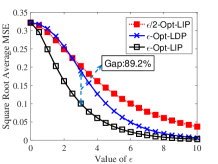
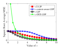
Refer to caption
(a) utility-privacy tradeoffs for website click aggregation with Karosak
Refer to caption
(b) utility-privacy tradeoffs for location tracking with Gowalla
Figure 9: Utility-privacy tradeoff comparisons using real world data

V-B2 Location Check-In Dataset

We then compare the performance of different models with another real-world dataset Gowalla, which is a social networking application where users share their locations by checking-in. There are 6,442,892 users in this dataset. For each user, a trace of his/her check-in locations are recorded. For this dataset, we wish to estimate a histogram of users’ last check-in location. We first divide the area into 36×36363636\times 36 districts. We then map each user’s locations into districts. Each user’s past check-in locations are used for calculating a global prior of the last check-in location for all the users. As studied in section. IV-C, for each user, the last check-in location is perturbed according to a MIMO-LIP (LDP) channel and a random vector is used for the adversary to estimate the histogram. The results are shown in Fig. 9(b), where similar trends can be observed as in the empirical results. Note that comparing with the theoretical results from Fig. 7, the advantage of LIP is even more clear in Fig. 9(b), that is because the theoretical analysis uses data from a domain with |𝔻|=20𝔻20|\mathbb{D}|=20. On the other hand, in the dataset of Gowalla, the input data is from a domain with |𝔻|=36×36𝔻3636|\mathbb{D}|=36\times{36}, even though many of the districts has o users checking-in, which results in zero priors for these districts. Based on the MIMO perturbation mechanism, for those districts with 0 prior, the system will also never output those districts, as a result, the data domain is equivalent to a much decreased one. Nevertheless, the effective domain size is |𝔻|=83𝔻83|\mathbb{D}|=83, which is much larger than 20. As we discussed, when domain size is large, the advantage of LIP is enhanced.

VI Conclusion and Future Work

In this paper, the notion of localized information privacy is proposed. As a context-aware privacy notion, it provides relaxed privacy guarantee than LDP by introducing prior knowledge in the privacy definition while achieving increased utility. Combined with an MMSE estimator which also leverages prior knowledge, larger gains in utility can be obtained. We studied the utility-privacy tradeoff of our proposed LIP notion and the traditional LDP notion under different both binary perturbation model and multiple-input and multiple-output perturbation model. In the binary model, we show that our ϵitalic-ϵ\epsilon-LIP always outperform ϵitalic-ϵ\epsilon-LDP for any given privacy budget ϵitalic-ϵ\epsilon. The advantage is more enhanced when the prior distribution is more skewed (even ϵ/2italic-ϵ2\epsilon/2-LIP with a stronger privacy guarantee than ϵitalic-ϵ\epsilon-LDP is better than the latter for small ϵitalic-ϵ\epsilon values). In the MIMO model, we show that when the input data has a larger range, both the LIP mechanisms and LDP mechanism suffer decreased utility. However, as the input range increasing, the decreased amount of the LIP mechanism is less than that of the LDP mechanism. Which means the context-aware privacy notion is more applicable than the context-free privacy notion in the MIMO case.

For future work, we will extend our work to handle more general models. For example, we will consider an adversary that has less accurate/complete prior knowledge than users, and also understand the impact of user correlations. We will also study the optimality of the perturbation model.

References

  • [1] B. Jiang, M. Li, and R. Tandon, “Context-Aware data aggregation with localized information privacy,” in 2018 IEEE Conference on Communications and Network Security (CNS) (IEEE CNS 2018), (Beijing, P.R. China), May 2018.
  • [2] P. Samarati and L. Sweeney, “Protecting privacy when disclosing information: k-anonymity and its enforcement through generalization and suppression,” tech. rep., 1998.
  • [3] C. Dwork, “Differential privacy: A survey of results,” in Theory and Applications of Models of Computation: 5th International Conference, TAMC (M. Agrawal, D. Du, and Z. Duan, eds.), pp. 1–19, 2008.
  • [4] C. Dwork, “Differential privacy,” in Automata, Languages and Programming: 33rd International Colloquium, ICALP 2006, Part II (M. Bugliesi, B. Preneel, V. Sassone, and I. Wegener, eds.), pp. 1–12, 2006.
  • [5] C. Dwork, F. McSherry, and K. Nissim, “Calibrating noise to sensitivity in private data analysis,” in Theory of Cryptography: Third Theory of Cryptography Conference, pp. 265–284, 2006.
  • [6] A. FITZPATRICK, “What to do after the massive yahoo hack,” 2016.
  • [7] R. Chen, H. Li, A. K. Qin, S. P. Kasiviswanathan, and H. Jin, “Private spatial data aggregation in the local setting,” in 2016 IEEE 32nd ICDE, pp. 289–300, May 2016.
  • [8] S. L. Warner, “Randomized response: A survey technique for eliminating evasive answer bias,” Journal of the American Statistical Association, vol. 60, no. 309, pp. 63–69, 1965.
  • [9] J. Freudiger, R. Shokri, and J.-P. Hubaux, “Evaluating the privacy risk of location-based services,” in Proceedings of the 15th International Conference on Financial Cryptography and Data Security, FC’11, (Berlin, Heidelberg), pp. 31–46, Springer-Verlag, 2012.
  • [10] P. Kairouz, S. Oh, and P. Viswanath, “Extremal mechanisms for local differential privacy,” in Advances in Neural Information Processing Systems 27, pp. 2879–2887, Curran Associates, Inc., 2014.
  • [11] A. D. Sarwate and L. Sankar, “A rate-disortion perspective on local differential privacy,” in 2014 52nd Annual Allerton Conference on Communication, Control, and Computing, pp. 903–908, Sept 2014.
  • [12] S. Xiong, A. D. Sarwate, and N. B. Mandayam, “Randomized requantization with local differential privacy,” in 2016 IEEE International Conference on Acoustics, Speech and Signal Processing (ICASSP), pp. 2189–2193, March 2016.
  • [13] Úlfar Erlingsson, V. Pihur, and A. Korolova, “Rappor: Randomized aggregatable privacy-preserving ordinal response,” in Proceedings of the 21st ACM CCCS, 2014.
  • [14] J. Tang, A. Korolova, X. Bai, X. Wang, and X. Wang, “Privacy loss in apple’s implementation of differential privacy on MacOS 10.12,” CoRR, vol. abs/1709.02753, 2017.
  • [15] T. Wang, J. Blocki, N. Li, and S. Jha, “Locally differentially private protocols for frequency estimation,” in 26th USENIX Security 17, pp. 729–745, USENIX Association, 2017.
  • [16] T.-H. H. Chan, E. Shi, and D. Song, “Optimal lower bound for differentially private multi-party aggregation,” in Proceedings of the 20th Annual ECA, ESA’12, pp. 277–288, 2012.
  • [17] R. Bassily, K. Nissim, U. Stemmer, and A. Thakurta, “Practical locally private heavy hitters,” CoRR, vol. abs/1707.04982, 2017.
  • [18] C. Huang, P. Kairouz, X. Chen, L. Sankar, and R. Rajagopal, “Context-aware generative adversarial privacy,” CoRR, vol. abs/1710.09549, 2017.
  • [19] W. Wang, L. Ying, and J. Zhang, “On the tradeoff between privacy and distortion in differential privacy,” CoRR, vol. abs/1402.3757, 2014.
  • [20] S. Asoodeh, F. Alajaji, and T. Linder, “Notes on information-theoretic privacy,” in 2014 52nd Allerton, pp. 1272–1278, Sept 2014.
  • [21] G. Wu and X. Xia, “Extending differential privacy for treating dependent records via information theory,” CoRR, vol. abs/1703.07474, 2017.
  • [22] W. Wang, L. Ying, and J. Zhang, “On the relation between identifiability, differential privacy, and mutual-information privacy,” IEEE Transactions on Information Theory, vol. 62, pp. 5018–5029, Sept 2016.
  • [23] S. Asoodeh, F. Alajaji, and T. Linder, “On maximal correlation, mutual information and data privacy,” in IEEE CWIT, pp. 27–31, July 2015.
  • [24] M. E. Andrés, N. E. Bordenabe, and K. Chatzikokolakis, “Geo-indistinguishability: Differential privacy for location-based systems,” CoRR, vol. abs/1212.1984, 2012.
  • [25] Y. Cao, M. Yoshikawa, Y. Xiao, and L. Xiong, “Quantifying differential privacy under temporal correlations,” in 2017 IEEE 33rd ICDE, pp. 821–832, April 2017.
  • [26] F. Tramèr and Z. Huang, “Differential privacy with bounded priors: Reconciling utility and privacy in genome-wide association studies,” in Proceedings of the 22Nd ACM SIGSAC, pp. 1286–1297, 2015.
  • [27] P. Kairouz, Oh, and Sewoong, “Extremal mechanisms for local differential privacy,” in Advances in Neural Information Processing Systems 27, pp. 2879–2887, 2014.
  • [28] F. Calmon and N. Fawaz, “Privacy against statistical inference,” 10 2012.
  • [29] F. A. S. Asoodeh and T. Linder, “Privacy-aware mmse estimation,” in 2016 IEEE ISIT, pp. 1989–1993, July 2016.
  • [30] Z. Qin, Y. Yang, and T. Yu, “Heavy hitter estimation over set-valued data with local differential privacy,” in Proceedings of the 2016 ACM SIGSAC, CCS ’16, pp. 192–203, 2016.
  • [31] A. Papoulis and S. Pillai, Probability, random variables, and stochastic processes. McGraw-Hill, 2002.

Appendix A Proof of theorem 2

Proof.
  1. 1.

    Step 1

    Notice that P1isubscriptsuperscript𝑃𝑖1P^{i}_{1} is a constant, thus the optimization problem is equivalent to maximize:

    Li(q0i,q1i)=superscript𝐿𝑖superscriptsubscript𝑞0𝑖superscriptsubscript𝑞1𝑖absent\displaystyle L^{i}(q_{0}^{i},q_{1}^{i})= (λ0iq1i)2λ0iλ1i=(λ1iq1iλ0i(1q1i))2λ0iλ1i.superscriptsubscriptsuperscript𝜆𝑖0superscriptsubscript𝑞1𝑖2subscriptsuperscript𝜆𝑖0subscriptsuperscript𝜆𝑖1superscriptsubscriptsuperscript𝜆𝑖1superscriptsubscript𝑞1𝑖subscriptsuperscript𝜆𝑖01superscriptsubscript𝑞1𝑖2subscriptsuperscript𝜆𝑖0subscriptsuperscript𝜆𝑖1\displaystyle\frac{(\lambda^{i}_{0}-q_{1}^{i})^{2}}{\lambda^{i}_{0}\lambda^{i}_{1}}=\frac{(\lambda^{i}_{1}q_{1}^{i}-\lambda^{i}_{0}(1-q_{1}^{i}))^{2}}{\lambda^{i}_{0}\lambda^{i}_{1}}. (43)

    In order to test the monotoncity of Li(q0i,q1i)superscript𝐿𝑖superscriptsubscript𝑞0𝑖superscriptsubscript𝑞1𝑖L^{i}(q_{0}^{i},q_{1}^{i}), taking partial derivative on it.

    Li(q0i,q1i)q0isuperscript𝐿𝑖superscriptsubscript𝑞0𝑖superscriptsubscript𝑞1𝑖superscriptsubscript𝑞0𝑖\displaystyle\frac{\partial{L^{i}(q_{0}^{i}},q_{1}^{i})}{\partial{q_{0}^{i}}} (44)
    =\displaystyle= (1q1i)2(λ0iλ1i)+q1i2(λ1iλ0i)+[2q1i(1q1i)]superscript1superscriptsubscript𝑞1𝑖2superscriptsubscriptsuperscript𝜆𝑖0subscriptsuperscript𝜆𝑖1superscriptsuperscriptsubscript𝑞1𝑖2superscriptsubscriptsuperscript𝜆𝑖1subscriptsuperscript𝜆𝑖0superscriptdelimited-[]2superscriptsubscript𝑞1𝑖1superscriptsubscript𝑞1𝑖\displaystyle(1-q_{1}^{i})^{2}(\frac{\lambda^{i}_{0}}{\lambda^{i}_{1}})^{\prime}+{{q_{1}^{i}}^{2}}(\frac{\lambda^{i}_{1}}{\lambda^{i}_{0}})^{\prime}+[-2q_{1}^{i}(1-q_{1}^{i})]^{\prime}
    =\displaystyle= (1q1i)2(P1i1λ1i2)+q1i2(1P1iλ0i2)superscript1superscriptsubscript𝑞1𝑖2subscriptsuperscript𝑃𝑖11superscriptsubscriptsuperscript𝜆𝑖12superscriptsuperscriptsubscript𝑞1𝑖21subscriptsuperscript𝑃𝑖1superscriptsubscriptsuperscript𝜆𝑖02\displaystyle(1-q_{1}^{i})^{2}(\frac{P^{i}_{1}-1}{{\lambda^{i}_{1}}^{2}})+{q_{1}^{i}}^{2}(\frac{1-P^{i}_{1}}{{\lambda^{i}_{0}}^{2}})
    =\displaystyle= (1P1i)((λ1iq1i)2[λ0i(1q1i)]2λ1i2λ0i2)1subscriptsuperscript𝑃𝑖1superscriptsubscriptsuperscript𝜆𝑖1superscriptsubscript𝑞1𝑖2superscriptdelimited-[]subscriptsuperscript𝜆𝑖01superscriptsubscript𝑞1𝑖2superscriptsubscriptsuperscript𝜆𝑖12superscriptsubscriptsuperscript𝜆𝑖02\displaystyle(1-P^{i}_{1})(\frac{(\lambda^{i}_{1}q_{1}^{i})^{2}-[\lambda^{i}_{0}(1-q_{1}^{i})]^{2}}{{\lambda^{i}_{1}}^{2}{\lambda^{i}_{0}}^{2}})
    =\displaystyle= (1P1i)[λ1iq1i+λ0i(1q1i)][λ1iq1iλ0i(1q1i)]λ1i2λ0i21subscriptsuperscript𝑃𝑖1delimited-[]subscriptsuperscript𝜆𝑖1superscriptsubscript𝑞1𝑖subscriptsuperscript𝜆𝑖01superscriptsubscript𝑞1𝑖delimited-[]subscriptsuperscript𝜆𝑖1superscriptsubscript𝑞1𝑖subscriptsuperscript𝜆𝑖01superscriptsubscript𝑞1𝑖superscriptsubscriptsuperscript𝜆𝑖12superscriptsubscriptsuperscript𝜆𝑖02\displaystyle(1-P^{i}_{1})\frac{[\lambda^{i}_{1}q_{1}^{i}+\lambda^{i}_{0}(1-q_{1}^{i})][\lambda^{i}_{1}q_{1}^{i}-\lambda^{i}_{0}(1-q_{1}^{i})]}{{\lambda^{i}_{1}}^{2}{\lambda^{i}_{0}}^{2}}
    =\displaystyle= (1P1i)2[λ1iq1i+λ0i(1q1i)](q1i+q0i1)λ1i2λ0i2.superscript1subscriptsuperscript𝑃𝑖12delimited-[]subscriptsuperscript𝜆𝑖1superscriptsubscript𝑞1𝑖subscriptsuperscript𝜆𝑖01superscriptsubscript𝑞1𝑖superscriptsubscript𝑞1𝑖superscriptsubscript𝑞0𝑖1superscriptsubscriptsuperscript𝜆𝑖12superscriptsubscriptsuperscript𝜆𝑖02\displaystyle(1-P^{i}_{1})^{2}\frac{[\lambda^{i}_{1}q_{1}^{i}+\lambda^{i}_{0}(1-q_{1}^{i})](q_{1}^{i}+q_{0}^{i}-1)}{{\lambda^{i}_{1}}^{2}{\lambda^{i}_{0}}^{2}}.

    In (45), noticed that Li(q0i,q1i)q0i0subscript𝐿𝑖superscriptsubscript𝑞0𝑖superscriptsubscript𝑞1𝑖superscriptsubscript𝑞0𝑖0\frac{\partial{L_{i}(q_{0}^{i}},q_{1}^{i})}{\partial{q_{0}^{i}}}\geq{0} when q1i+q0i10superscriptsubscript𝑞1𝑖superscriptsubscript𝑞0𝑖10q_{1}^{i}+q_{0}^{i}-1\geq{0}; Li(q0i,q1i)q0i<0subscript𝐿𝑖superscriptsubscript𝑞0𝑖superscriptsubscript𝑞1𝑖superscriptsubscript𝑞0𝑖0\frac{\partial{L_{i}(q_{0}^{i}},q_{1}^{i})}{\partial{q_{0}^{i}}}<{0} when q1i+q0i1<0superscriptsubscript𝑞1𝑖superscriptsubscript𝑞0𝑖10q_{1}^{i}+q_{0}^{i}-1<{0}. Which means given any value of q1isuperscriptsubscript𝑞1𝑖q_{1}^{i}, Li(q0i,q1i)superscript𝐿𝑖superscriptsubscript𝑞0𝑖superscriptsubscript𝑞1𝑖L^{i}(q_{0}^{i},q_{1}^{i}) is monotonically decreasing with q0isuperscriptsubscript𝑞0𝑖q_{0}^{i} from 0 to 1q1i1superscriptsubscript𝑞1𝑖1-q_{1}^{i}.
    By the same way, when q0isuperscriptsubscript𝑞0𝑖q_{0}^{i} is fixed, Li(q0i,q1i)subscript𝐿𝑖superscriptsubscript𝑞0𝑖superscriptsubscript𝑞1𝑖L_{i}(q_{0}^{i},q_{1}^{i}) is monotonically decreasing with q1isuperscriptsubscript𝑞1𝑖q_{1}^{i} from 0 to 1q0i1superscriptsubscript𝑞0𝑖1-q_{0}^{i}.

  2. 2.

    Step 2

    To test the symmetry of Li(q0i,q1i)subscript𝐿𝑖superscriptsubscript𝑞0𝑖superscriptsubscript𝑞1𝑖L_{i}(q_{0}^{i},q_{1}^{i}), take q0i=1q0isuperscriptsubscript𝑞0superscript𝑖1superscriptsubscript𝑞0𝑖q_{0}^{i^{\prime}}=1-q_{0}^{i}, q1i=1q1isuperscriptsubscript𝑞1superscript𝑖1superscriptsubscript𝑞1𝑖q_{1}^{i^{\prime}}=1-q_{1}^{i}.

    Li(q0i,q1i)=superscript𝐿𝑖superscriptsubscript𝑞0superscript𝑖superscriptsubscript𝑞1superscript𝑖absent\displaystyle L^{i}(q_{0}^{i^{\prime}},q_{1}^{i^{\prime}})= (1P1i)2(1q0iq1i)2λ1iλ0isuperscript1subscriptsuperscript𝑃𝑖12superscript1superscriptsubscript𝑞0𝑖superscriptsubscript𝑞1𝑖2subscriptsuperscript𝜆𝑖1subscriptsuperscript𝜆𝑖0\displaystyle\frac{(1-P^{i}_{1})^{2}(1-q_{0}^{i}-q_{1}^{i})^{2}}{\lambda^{i}_{1}\lambda^{i}_{0}}
    =\displaystyle= Li(q0i,q1i).superscript𝐿𝑖superscriptsubscript𝑞0𝑖superscriptsubscript𝑞1𝑖\displaystyle L^{i}(q_{0}^{i},q_{1}^{i}).

    Thus, Li(q0i,q1i)superscript𝐿𝑖superscriptsubscript𝑞0𝑖superscriptsubscript𝑞1𝑖L^{i}(q_{0}^{i},q_{1}^{i}) is symmetric about (0.5,0.5)0.50.5(0.5,0.5), which means for every point (q0i,q1i)superscriptsubscript𝑞0𝑖superscriptsubscript𝑞1𝑖(q_{0}^{i},q_{1}^{i}) on the left of q0i+q1i=1superscriptsubscript𝑞0𝑖superscriptsubscript𝑞1𝑖1q_{0}^{i}+q_{1}^{i}=1, we can find a point on the right side of q0i+q1i=1superscriptsubscript𝑞0𝑖superscriptsubscript𝑞1𝑖1q_{0}^{i}+q_{1}^{i}=1 that result in a same Li(q0i,q1i)superscript𝐿𝑖superscriptsubscript𝑞0𝑖superscriptsubscript𝑞1𝑖L^{i}(q_{0}^{i},q_{1}^{i}) value.

    In terms of the constraints, first derive F1i(q0i,q1i)subscriptsuperscript𝐹𝑖1superscriptsubscript𝑞0𝑖superscriptsubscript𝑞1𝑖F^{i}_{1}(q_{0}^{i},q_{1}^{i}), F2i(q0i,q1i)subscriptsuperscript𝐹𝑖2superscriptsubscript𝑞0𝑖superscriptsubscript𝑞1𝑖F^{i}_{2}(q_{0}^{i},q_{1}^{i}), F3i(q0i,q1i)subscriptsuperscript𝐹𝑖3superscriptsubscript𝑞0𝑖superscriptsubscript𝑞1𝑖F^{i}_{3}(q_{0}^{i},q_{1}^{i}), F4i(q0i,q1i)subscriptsuperscript𝐹𝑖4superscriptsubscript𝑞0𝑖superscriptsubscript𝑞1𝑖F^{i}_{4}(q_{0}^{i},q_{1}^{i}) as:

    F1i(q0i,q1i)=subscriptsuperscript𝐹𝑖1superscriptsubscript𝑞0𝑖superscriptsubscript𝑞1𝑖absent\displaystyle F^{i}_{1}(q_{0}^{i},q_{1}^{i})= Pr(X=1)Pr(X=1|Y=0)=λ0iq1i;𝑃𝑟𝑋1𝑃𝑟𝑋conditional1𝑌0subscriptsuperscript𝜆𝑖0subscriptsuperscript𝑞𝑖1\displaystyle\frac{Pr(X=1)}{Pr(X=1|Y=0)}=\frac{\lambda^{i}_{0}}{q^{i}_{1}}; (45)
    F2i(q0i,q1i)=subscriptsuperscript𝐹𝑖2superscriptsubscript𝑞0𝑖superscriptsubscript𝑞1𝑖absent\displaystyle F^{i}_{2}(q_{0}^{i},q_{1}^{i})= Pr(X=1)Pr(X=1|Y=1)=λ1i1q1i;𝑃𝑟𝑋1𝑃𝑟𝑋conditional1𝑌1subscriptsuperscript𝜆𝑖11subscriptsuperscript𝑞𝑖1\displaystyle\frac{Pr(X=1)}{Pr(X=1|Y=1)}=\frac{\lambda^{i}_{1}}{1-q^{i}_{1}};
    F3i(q0i,q1i)=subscriptsuperscript𝐹𝑖3superscriptsubscript𝑞0𝑖superscriptsubscript𝑞1𝑖absent\displaystyle F^{i}_{3}(q_{0}^{i},q_{1}^{i})= Pr(X=0)Pr(X=0|Y=0)=λ0i1q0i;𝑃𝑟𝑋0𝑃𝑟𝑋conditional0𝑌0subscriptsuperscript𝜆𝑖01subscriptsuperscript𝑞𝑖0\displaystyle\frac{Pr(X=0)}{Pr(X=0|Y=0)}=\frac{\lambda^{i}_{0}}{1-q^{i}_{0}};
    F4i(q0i,q1i)=subscriptsuperscript𝐹𝑖4superscriptsubscript𝑞0𝑖superscriptsubscript𝑞1𝑖absent\displaystyle F^{i}_{4}(q_{0}^{i},q_{1}^{i})= Pr(X=0)Pr(X=0|Y=1)=λ1iq0i.𝑃𝑟𝑋0𝑃𝑟𝑋conditional0𝑌1subscriptsuperscript𝜆𝑖1subscriptsuperscript𝑞𝑖0\displaystyle\frac{Pr(X=0)}{Pr(X=0|Y=1)}=\frac{\lambda^{i}_{1}}{q^{i}_{0}}.

    if taking q0i=1q0isuperscriptsubscript𝑞0superscript𝑖1superscriptsubscript𝑞0𝑖q_{0}^{i^{\prime}}=1-q_{0}^{i}, q1i=1q1isuperscriptsubscript𝑞1superscript𝑖1superscriptsubscript𝑞1𝑖q_{1}^{i^{\prime}}=1-q_{1}^{i} into F1i(q0i,q1i)subscriptsuperscript𝐹𝑖1superscriptsubscript𝑞0𝑖superscriptsubscript𝑞1𝑖F^{i}_{1}(q_{0}^{i},q_{1}^{i}), F2i(q0i,q1i)subscriptsuperscript𝐹𝑖2superscriptsubscript𝑞0𝑖superscriptsubscript𝑞1𝑖F^{i}_{2}(q_{0}^{i},q_{1}^{i}), F3i(q0i,q1i)subscriptsuperscript𝐹𝑖3superscriptsubscript𝑞0𝑖superscriptsubscript𝑞1𝑖F^{i}_{3}(q_{0}^{i},q_{1}^{i}) and F4i(q0i,q1i)subscriptsuperscript𝐹𝑖4superscriptsubscript𝑞0𝑖superscriptsubscript𝑞1𝑖F^{i}_{4}(q_{0}^{i},q_{1}^{i}):

    F1i(q0i,q1i)=λ1i1q1i=F2i(q0i,q1i),subscriptsuperscript𝐹𝑖1superscriptsubscript𝑞0superscript𝑖superscriptsubscript𝑞1superscript𝑖subscriptsuperscript𝜆𝑖11superscriptsubscript𝑞1𝑖subscriptsuperscript𝐹𝑖2superscriptsubscript𝑞0𝑖superscriptsubscript𝑞1𝑖F^{i}_{1}(q_{0}^{i^{\prime}},q_{1}^{i^{\prime}})=\frac{\lambda^{i}_{1}}{1-q_{1}^{i}}=F^{i}_{2}(q_{0}^{i},q_{1}^{i}),
    F2i(q0i,q1i)=λ0iq1i=F1i(q0i,q1i),subscriptsuperscript𝐹𝑖2superscriptsubscript𝑞0superscript𝑖superscriptsubscript𝑞1superscript𝑖subscriptsuperscript𝜆𝑖0superscriptsubscript𝑞1𝑖subscriptsuperscript𝐹𝑖1superscriptsubscript𝑞0𝑖superscriptsubscript𝑞1𝑖F^{i}_{2}(q_{0}^{i^{\prime}},q_{1}^{i^{\prime}})=\frac{\lambda^{i}_{0}}{q_{1}^{i}}=F^{i}_{1}(q_{0}^{i},q_{1}^{i}),
    F3i(q0i,q1i)=λ1iq0i=F4i(q0i,q1i),subscriptsuperscript𝐹𝑖3superscriptsubscript𝑞0superscript𝑖superscriptsubscript𝑞1superscript𝑖subscriptsuperscript𝜆𝑖1superscriptsubscript𝑞0𝑖subscriptsuperscript𝐹𝑖4superscriptsubscript𝑞0𝑖superscriptsubscript𝑞1𝑖F^{i}_{3}(q_{0}^{i^{\prime}},q_{1}^{i^{\prime}})=\frac{\lambda^{i}_{1}}{q_{0}^{i}}=F^{i}_{4}(q_{0}^{i},q_{1}^{i}),
    F4i(q0i,q1i)=λ0i1q0i=F1i(q0i,q1i).subscriptsuperscript𝐹𝑖4superscriptsubscript𝑞0superscript𝑖superscriptsubscript𝑞1superscript𝑖subscriptsuperscript𝜆𝑖01superscriptsubscript𝑞0𝑖subscriptsuperscript𝐹𝑖1superscriptsubscript𝑞0𝑖superscriptsubscript𝑞1𝑖F^{i}_{4}(q_{0}^{i^{\prime}},q_{1}^{i^{\prime}})=\frac{\lambda^{i}_{0}}{1-q_{0}^{i}}=F^{i}_{1}(q_{0}^{i},q_{1}^{i}).

    As a result, the four constraints functions are symmetric about point (0.5,0.5)0.50.5(0.5,0.5). Assume that Fji(q0i,q1i)subscriptsuperscript𝐹𝑖𝑗superscriptsubscript𝑞0𝑖superscriptsubscript𝑞1𝑖F^{i}_{j}(q_{0}^{i},q_{1}^{i}), j=1,2,3,4𝑗1234j=1,2,3,4 form a feasible region 𝒯isubscript𝒯𝑖\mathcal{T}_{i} for (q0i,q1i)superscriptsubscript𝑞0𝑖superscriptsubscript𝑞1𝑖(q_{0}^{i},q_{1}^{i}), thus for any point in this region, another point can be found on the other side of q0i+q1i=1superscriptsubscript𝑞0𝑖superscriptsubscript𝑞1𝑖1q_{0}^{i}+q_{1}^{i}=1 also in 𝒯isubscript𝒯𝑖\mathcal{T}_{i}. Now (q0i,q1i)𝒯i=𝒯i{q0i+q1i1}superscriptsubscript𝑞0𝑖superscriptsubscript𝑞1𝑖subscript𝒯𝑖subscript𝒯𝑖superscriptsubscript𝑞0𝑖superscriptsubscript𝑞1𝑖1(q_{0}^{i*},q_{1}^{i*})\in{\mathcal{T}_{i}=\mathcal{T}_{i}\cap\{{q_{0}^{i}+q_{1}^{i}\leq{1}}\}}.

    Fig. LABEL:contour illustrates the function of Li(q0i,q1i)subscript𝐿𝑖superscriptsubscript𝑞0𝑖superscriptsubscript𝑞1𝑖L_{i}(q_{0}^{i},q_{1}^{i}) and feasible region isuperscript𝑖\mathcal{R}^{i} on the plane of q0i,q1isuperscriptsubscript𝑞0𝑖superscriptsubscript𝑞1𝑖q_{0}^{i},q_{1}^{i}, curves in the figure is the contour line of Li(q0i,q1i)subscript𝐿𝑖superscriptsubscript𝑞0𝑖superscriptsubscript𝑞1𝑖L_{i}(q_{0}^{i},q_{1}^{i}), while the shadow region is the feasible region of 𝒯isubscript𝒯𝑖\mathcal{T}_{i} when ϵitalic-ϵ\epsilon is fixed.

  3. 3.

    Step 3

    Since

    F1iF2i=subscriptsuperscript𝐹𝑖1subscriptsuperscript𝐹𝑖2absent\displaystyle F^{i}_{1}-F^{i}_{2}= P1i+(1P1i)(1q0i)q1i(P1i+(1P1i)q0i1q1i)subscriptsuperscript𝑃𝑖11subscriptsuperscript𝑃𝑖11subscriptsuperscript𝑞𝑖0subscriptsuperscript𝑞𝑖1subscriptsuperscript𝑃𝑖11subscriptsuperscript𝑃𝑖1subscriptsuperscript𝑞𝑖01subscriptsuperscript𝑞𝑖1\displaystyle P^{i}_{1}+\frac{(1-P^{i}_{1})(1-q^{i}_{0})}{q^{i}_{1}}-(P^{i}_{1}+\frac{(1-P^{i}_{1})q^{i}_{0}}{1-q^{i}_{1}})
    =\displaystyle= (1P1i)1q0iq1iq1i(1q1i)1subscriptsuperscript𝑃𝑖11subscriptsuperscript𝑞𝑖0subscriptsuperscript𝑞𝑖1subscriptsuperscript𝑞𝑖11subscriptsuperscript𝑞𝑖1\displaystyle(1-P^{i}_{1})\frac{1-q^{i}_{0}-q^{i}_{1}}{q^{i}_{1}(1-q^{i}_{1})}

    and

    F4iF3i=subscriptsuperscript𝐹𝑖4subscriptsuperscript𝐹𝑖3absent\displaystyle F^{i}_{4}-F^{i}_{3}= 1P1i+P1i(1q1i)q0i(1P1i+P1iq1i1q0i)1subscriptsuperscript𝑃𝑖1subscriptsuperscript𝑃𝑖11subscriptsuperscript𝑞𝑖1subscriptsuperscript𝑞𝑖01subscriptsuperscript𝑃𝑖1subscriptsuperscript𝑃𝑖1subscriptsuperscript𝑞𝑖11subscriptsuperscript𝑞𝑖0\displaystyle 1-P^{i}_{1}+\frac{P^{i}_{1}(1-q^{i}_{1})}{q^{i}_{0}}-(1-P^{i}_{1}+\frac{P^{i}_{1}q^{i}_{1}}{1-q^{i}_{0}})
    =\displaystyle= (1P1i)1q0iq1iq1i(1q1i),1subscriptsuperscript𝑃𝑖11subscriptsuperscript𝑞𝑖0subscriptsuperscript𝑞𝑖1subscriptsuperscript𝑞𝑖11subscriptsuperscript𝑞𝑖1\displaystyle(1-P^{i}_{1})\frac{1-q^{i}_{0}-q^{i}_{1}}{q^{i}_{1}(1-q^{i}_{1})},

    for any point (q0i,q1i)𝒯isuperscriptsubscript𝑞0𝑖superscriptsubscript𝑞1𝑖subscript𝒯𝑖(q_{0}^{i},q_{1}^{i})\in{\mathcal{T}_{i}}, there is F1iF2isubscriptsuperscript𝐹𝑖1subscriptsuperscript𝐹𝑖2F^{i}_{1}\geq{F^{i}_{2}} and F4iF3isubscriptsuperscript𝐹𝑖4subscriptsuperscript𝐹𝑖3F^{i}_{4}\geq{F^{i}_{3}}

    𝒯i={F1ieϵ}subscript𝒯𝑖subscriptsuperscript𝐹𝑖1superscript𝑒italic-ϵ\displaystyle\mathcal{T}_{i}=\{F^{i}_{1}\leq{e^{\epsilon}}\} {eϵF2i}{eϵF3i}superscript𝑒italic-ϵsubscriptsuperscript𝐹𝑖2superscript𝑒italic-ϵsubscriptsuperscript𝐹𝑖3\displaystyle\cap\{e^{-\epsilon}\leq{F^{i}_{2}}\}\cap\{e^{-\epsilon}\leq{F^{i}_{3}}\} (46)
    {F4ieϵ}{q0i+q1i1}subscriptsuperscript𝐹𝑖4superscript𝑒italic-ϵsuperscriptsubscript𝑞0𝑖superscriptsubscript𝑞1𝑖1\displaystyle\cap\{F^{i}_{4}\leq{e^{\epsilon}}\}\cap\{{q_{0}^{i}+q_{1}^{i}\leq{1}}\}

    From (46), assume that q0isuperscriptsubscript𝑞0𝑖q_{0}^{i} is fixed to be q0subscript𝑞0q_{0}, then

    q1i{(1P1i)(1q0)eϵP1iifq0P1i/eϵ1(eϵ+P1i1)(q0)P1iifq0<P1i/eϵ.superscriptsubscript𝑞1𝑖cases1subscriptsuperscript𝑃𝑖11subscript𝑞0superscript𝑒italic-ϵsubscriptsuperscript𝑃𝑖1𝑖𝑓subscript𝑞0subscriptsuperscript𝑃𝑖1superscript𝑒italic-ϵ1superscript𝑒italic-ϵsubscriptsuperscript𝑃𝑖11subscript𝑞0subscriptsuperscript𝑃𝑖1𝑖𝑓subscript𝑞0subscriptsuperscript𝑃𝑖1superscript𝑒italic-ϵq_{1}^{i}\geq\begin{cases}\frac{(1-P^{i}_{1})(1-q_{0})}{e^{\epsilon}-P^{i}_{1}}&if\quad{q_{0}\geq{P^{i}_{1}/e^{\epsilon}}}\\ 1-\frac{(e^{\epsilon}+P^{i}_{1}-1)(q_{0})}{P^{i}_{1}}&if\quad{q_{0}<{P^{i}_{1}/e^{\epsilon}}}.\end{cases}

    Since Li(q0i,q1i)superscript𝐿𝑖superscriptsubscript𝑞0𝑖superscriptsubscript𝑞1𝑖L^{i}(q_{0}^{i},q_{1}^{i}) is monotonically decreasing with q0isuperscriptsubscript𝑞0𝑖q_{0}^{i} and q1isuperscriptsubscript𝑞1𝑖q_{1}^{i} in 𝒯isubscript𝒯𝑖\mathcal{T}_{i}, For any q0isuperscriptsubscript𝑞0𝑖q_{0}^{i} in 𝒯isubscript𝒯𝑖\mathcal{T}_{i}, its according optimal q1isuperscriptsubscript𝑞1𝑖q_{1}^{i*} is the smallest value s.t. (q0i,q1i)superscriptsubscript𝑞0𝑖superscriptsubscript𝑞1𝑖(q_{0}^{i},q_{1}^{i*}) is in 𝒯isubscript𝒯𝑖\mathcal{T}_{i}. It is the same with q0isuperscriptsubscript𝑞0𝑖q_{0}^{i*}. On the other hand, F1isubscriptsuperscript𝐹𝑖1F^{i}_{1}, F2isubscriptsuperscript𝐹𝑖2F^{i}_{2}, F3isubscriptsuperscript𝐹𝑖3F^{i}_{3}, F4isubscriptsuperscript𝐹𝑖4F^{i}_{4} are all liner, their bounds value can be achieved when they are equal to their constraints values eϵsuperscript𝑒italic-ϵe^{\epsilon} or eϵsuperscript𝑒italic-ϵe^{-\epsilon}. As a result,

    (q0i,q1i){{F1i=eϵ}ifq0P1i/eϵ{F4i=eϵ}ifq0<P1i/eϵ.subscriptsuperscript𝑞𝑖0subscriptsuperscript𝑞𝑖1casessubscriptsuperscript𝐹𝑖1superscript𝑒italic-ϵ𝑖𝑓subscript𝑞0subscriptsuperscript𝑃𝑖1superscript𝑒italic-ϵsubscriptsuperscript𝐹𝑖4superscript𝑒italic-ϵ𝑖𝑓subscript𝑞0subscriptsuperscript𝑃𝑖1superscript𝑒italic-ϵ(q^{i*}_{0},q^{i*}_{1})\in\begin{cases}\{F^{i}_{1}={e^{\epsilon}}\}&if\quad{q_{0}\geq{P^{i}_{1}/e^{\epsilon}}}\\ \{F^{i}_{4}={e^{\epsilon}}\}&if\quad{q_{0}<{P^{i}_{1}/e^{\epsilon}}}.\end{cases}
  4. 4.

    Step 4

    To find the minimal value of Li(q0i,q1i)superscript𝐿𝑖superscriptsubscript𝑞0𝑖superscriptsubscript𝑞1𝑖L^{i}(q_{0}^{i},q_{1}^{i}), where (q0i,q1i)𝒯isuperscriptsubscript𝑞0𝑖superscriptsubscript𝑞1𝑖subscript𝒯𝑖(q_{0}^{i},q_{1}^{i})\in\mathcal{T}_{i}, the last thing we need to do is to test its monotocity of Li(q0i,q1i)superscript𝐿𝑖superscriptsubscript𝑞0𝑖superscriptsubscript𝑞1𝑖L^{i}(q_{0}^{i},q_{1}^{i}) given F1i=eϵsubscriptsuperscript𝐹𝑖1superscript𝑒italic-ϵF^{i}_{1}={e^{\epsilon}} or F4i=eϵsubscriptsuperscript𝐹𝑖4superscript𝑒italic-ϵF^{i}_{4}=e^{\epsilon}.

    LF1i=eϵi(q0i,q1i)=subscriptsuperscript𝐿𝑖subscriptsuperscript𝐹𝑖1superscript𝑒italic-ϵsuperscriptsubscript𝑞0𝑖superscriptsubscript𝑞1𝑖absent\displaystyle L^{i}_{F^{i}_{1}={e^{\epsilon}}}(q_{0}^{i},q_{1}^{i})= (1P1i)2(q0i+q1i1)2λ0iλ1isuperscript1subscriptsuperscript𝑃𝑖12superscriptsuperscriptsubscript𝑞0𝑖superscriptsubscript𝑞1𝑖12subscriptsuperscript𝜆𝑖0subscriptsuperscript𝜆𝑖1\displaystyle\frac{(1-P^{i}_{1})^{2}(q_{0}^{i}+q_{1}^{i}-1)^{2}}{\lambda^{i}_{0}\lambda^{i}_{1}}
    =\displaystyle= [(1P1i)(eϵ1)q1i]2λ0iλ1i,superscriptdelimited-[]1subscriptsuperscript𝑃𝑖1superscript𝑒italic-ϵ1superscriptsubscript𝑞1𝑖2subscriptsuperscript𝜆𝑖0subscriptsuperscript𝜆𝑖1\displaystyle\frac{[(1-P^{i}_{1})(e^{\epsilon}-1)q_{1}^{i}]^{2}}{\lambda^{i}_{0}\lambda^{i}_{1}},

    To find the minimal value, taking derivative over LF1i=eϵisubscriptsuperscript𝐿𝑖subscriptsuperscript𝐹𝑖1superscript𝑒italic-ϵL^{i}_{F^{i}_{1}={e^{\epsilon}}}

    LF1i=eϵi(q0i,q1i)q1isubscriptsuperscript𝐿𝑖subscriptsuperscript𝐹𝑖1superscript𝑒italic-ϵsuperscriptsubscript𝑞0𝑖superscriptsubscript𝑞1𝑖superscriptsubscript𝑞1𝑖\displaystyle\frac{\partial{L^{i}_{F^{i}_{1}={e^{\epsilon}}}(q_{0}^{i},q_{1}^{i})}}{\partial{q_{1}^{i}}}
    =\displaystyle= (1P1i)2(eϵ1)2(q1i2λ0iλ1i)superscript1subscriptsuperscript𝑃𝑖12superscriptsuperscript𝑒italic-ϵ12superscriptsuperscriptsuperscriptsubscript𝑞1𝑖2subscriptsuperscript𝜆𝑖0subscriptsuperscript𝜆𝑖1\displaystyle(1-P^{i}_{1})^{2}(e^{\epsilon}-1)^{2}(\frac{{q_{1}^{i}}^{2}}{\lambda^{i}_{0}\lambda^{i}_{1}})^{\prime}
    =\displaystyle= (1P1i)2(eϵ1)2q1iλ1i(λ0iP1iq1i)+λ0iλ1i+P1iq1iλ0i(λ0iλ1i)2superscript1subscriptsuperscript𝑃𝑖12superscriptsuperscript𝑒italic-ϵ12superscriptsubscript𝑞1𝑖subscriptsuperscript𝜆𝑖1subscriptsuperscript𝜆𝑖0subscriptsuperscript𝑃𝑖1subscriptsuperscript𝑞𝑖1subscriptsuperscript𝜆𝑖0subscriptsuperscript𝜆𝑖1subscriptsuperscript𝑃𝑖1subscriptsuperscript𝑞𝑖1subscriptsuperscript𝜆𝑖0superscriptsubscriptsuperscript𝜆𝑖0subscriptsuperscript𝜆𝑖12\displaystyle(1-P^{i}_{1})^{2}(e^{\epsilon}-1)^{2}{q_{1}^{i}}\frac{\lambda^{i}_{1}(\lambda^{i}_{0}-P^{i}_{1}q^{i}_{1})+\lambda^{i}_{0}\lambda^{i}_{1}+P^{i}_{1}q^{i}_{1}\lambda^{i}_{0}}{(\lambda^{i}_{0}\lambda^{i}_{1})^{2}}

    Which is obviously greater than 0, similarly, when F4i=eϵsubscriptsuperscript𝐹𝑖4superscript𝑒italic-ϵF^{i}_{4}=e^{\epsilon} is given:

    LF4i=eϵi(q0i,q1i)q0isubscriptsuperscript𝐿𝑖subscriptsuperscript𝐹𝑖4superscript𝑒italic-ϵsuperscriptsubscript𝑞0𝑖superscriptsubscript𝑞1𝑖superscriptsubscript𝑞0𝑖\displaystyle\frac{\partial{L^{i}_{F^{i}_{4}={e^{\epsilon}}}(q_{0}^{i},q_{1}^{i})}}{\partial{q_{0}^{i}}}
    =\displaystyle= P1i2(eϵ1)2(q0i2λ0iλ1i)superscriptsubscriptsuperscript𝑃𝑖12superscriptsuperscript𝑒italic-ϵ12superscriptsuperscriptsuperscriptsubscript𝑞0𝑖2subscriptsuperscript𝜆𝑖0subscriptsuperscript𝜆𝑖1\displaystyle{P^{i}_{1}}^{2}(e^{\epsilon}-1)^{2}(\frac{{q_{0}^{i}}^{2}}{\lambda^{i}_{0}\lambda^{i}_{1}})^{\prime}
    =\displaystyle= P1i2(eϵ1)2q0iλ0i(λ1i(1P1i)q0i)+λ1i(1P1i)q0i(λ0iλ1i)2superscriptsubscriptsuperscript𝑃𝑖12superscriptsuperscript𝑒italic-ϵ12superscriptsubscript𝑞0𝑖subscriptsuperscript𝜆𝑖0subscriptsuperscript𝜆𝑖11subscriptsuperscript𝑃𝑖1subscriptsuperscript𝑞𝑖0subscriptsuperscript𝜆𝑖11subscriptsuperscript𝑃𝑖1subscriptsuperscript𝑞𝑖0superscriptsubscriptsuperscript𝜆𝑖0subscriptsuperscript𝜆𝑖12\displaystyle{P^{i}_{1}}^{2}(e^{\epsilon}-1)^{2}{q_{0}^{i}}\frac{\lambda^{i}_{0}(\lambda^{i}_{1}-(1-P^{i}_{1})q^{i}_{0})+\lambda^{i}_{1}(1-P^{i}_{1})q^{i}_{0}}{(\lambda^{i}_{0}\lambda^{i}_{1})^{2}}

    Which is also greater then 0. Noticed that, when q0iP1ieϵsuperscriptsubscript𝑞0𝑖subscriptsuperscript𝑃𝑖1superscript𝑒italic-ϵq_{0}^{i}\leq{\frac{P^{i}_{1}}{e^{\epsilon}}}, optimal point is (q0i,q1i)=(P1ieϵ,1P1ieϵ)subscriptsuperscript𝑞𝑖0subscriptsuperscript𝑞𝑖1subscriptsuperscript𝑃𝑖1superscript𝑒italic-ϵ1subscriptsuperscript𝑃𝑖1superscript𝑒italic-ϵ(q^{i*}_{0},q^{i*}_{1})=(\frac{P^{i}_{1}}{e^{\epsilon}},\frac{1-P^{i}_{1}}{e^{\epsilon}}), when q0i>P1ieϵsuperscriptsubscript𝑞0𝑖subscriptsuperscript𝑃𝑖1superscript𝑒italic-ϵq_{0}^{i}>{\frac{P^{i}_{1}}{e^{\epsilon}}}, the optimal point is also (q0i,q1i)=(P1ieϵ,1P1ieϵ)subscriptsuperscript𝑞𝑖0subscriptsuperscript𝑞𝑖1subscriptsuperscript𝑃𝑖1superscript𝑒italic-ϵ1subscriptsuperscript𝑃𝑖1superscript𝑒italic-ϵ(q^{i*}_{0},q^{i*}_{1})=(\frac{P^{i}_{1}}{e^{\epsilon}},\frac{1-P^{i}_{1}}{e^{\epsilon}}). Thus the global optimal solution is (P1ieϵ,1P1ieϵ)subscriptsuperscript𝑃𝑖1superscript𝑒italic-ϵ1subscriptsuperscript𝑃𝑖1superscript𝑒italic-ϵ(\frac{P^{i}_{1}}{e^{\epsilon}},\frac{1-P^{i}_{1}}{e^{\epsilon}}).

Appendix B Proof of Theorem 3

Proof.

Notice that Var[Xi]𝑉𝑎𝑟delimited-[]subscript𝑋𝑖Var[X_{i}] is a non-negative constant, thus minizing MSE is equivalent to maximize Var[Xi^]𝑉𝑎𝑟delimited-[]^subscript𝑋𝑖Var[\hat{X_{i}}].

Lemma 1.

Regardless of the privacy constraints, one set of solutions of 𝐪𝐢superscript𝐪𝐢\mathbf{q^{i}} that result in the minimal value of Var[Xi^]𝑉𝑎𝑟delimited-[]^subscript𝑋𝑖Var[\hat{X_{i}}] is qnki=λkisubscriptsuperscript𝑞𝑖𝑛𝑘subscriptsuperscript𝜆𝑖𝑘q^{i}_{nk}=\lambda^{i}_{k}, n,k1,2,3dformulae-sequencefor-all𝑛𝑘123𝑑\forall{n,k\in{1,2,3...d}}; one set of solutions of 𝐪𝐢superscript𝐪𝐢\mathbf{q^{i}} that result in the maximal value of Var[Xi^]𝑉𝑎𝑟delimited-[]^subscript𝑋𝑖Var[\hat{X_{i}}] is all qkjisubscriptsuperscript𝑞𝑖𝑘𝑗q^{i}_{kj}s are from the set of {0,1}01\{0,1\}, and for any nm𝑛𝑚n\neq{m}, qnjisubscriptsuperscript𝑞𝑖𝑛𝑗q^{i}_{nj} and qmjisubscriptsuperscript𝑞𝑖𝑚𝑗q^{i}_{mj} can not be 1 simultaneously.

Proof.

Obviously, minimized solution:
Consider a set of parameters: 𝐪𝐦𝐢𝐧𝐢superscriptsubscript𝐪𝐦𝐢𝐧𝐢\mathbf{q_{min}^{i}}, when qnki=λkisubscriptsuperscript𝑞𝑖𝑛𝑘subscriptsuperscript𝜆𝑖𝑘q^{i}_{nk}=\lambda^{i}_{k}, n,k1,2,3dformulae-sequencefor-all𝑛𝑘123𝑑\forall{n,k\in{1,2,3...d}}, Var[Xi^]=0𝑉𝑎𝑟delimited-[]^subscript𝑋𝑖0Var[\hat{X_{i}}]=0, as Var[Xi^]0𝑉𝑎𝑟delimited-[]^subscript𝑋𝑖0Var[\hat{X_{i}}]\geq 0, thus qnki=λkisubscriptsuperscript𝑞𝑖𝑛𝑘subscriptsuperscript𝜆𝑖𝑘q^{i}_{nk}=\lambda^{i}_{k} results in a minimal value of Var[Xi^]𝑉𝑎𝑟delimited-[]^subscript𝑋𝑖Var[\hat{X_{i}}].
On the other hand, maximized solution: Consider a set of parameters: 𝐪𝐦𝐚𝐱𝐢superscriptsubscript𝐪𝐦𝐚𝐱𝐢\mathbf{q_{max}^{i}}, assume that for all n1,2d𝑛12𝑑n\in{1,2...d}, there’s a k1,2,,d𝑘12𝑑k\in{1,2,...,d}, such that qnki=1subscriptsuperscript𝑞𝑖𝑛𝑘1q^{i}_{nk}=1 and qnli=0subscriptsuperscript𝑞𝑖𝑛𝑙0q^{i}_{nl}=0 for all lk𝑙𝑘l\neq{k} and for different n𝑛n, k𝑘k is different, thus λki=Pnisubscriptsuperscript𝜆𝑖𝑘subscriptsuperscript𝑃𝑖𝑛\lambda^{i}_{k}=P^{i}_{n}

m=1dn=1dk=1damanPmiPniqmki(qnkiλki1)subscriptsuperscript𝑑𝑚1subscriptsuperscript𝑑𝑛1subscriptsuperscript𝑑𝑘1subscript𝑎𝑚subscript𝑎𝑛subscriptsuperscript𝑃𝑖𝑚subscriptsuperscript𝑃𝑖𝑛subscriptsuperscript𝑞𝑖𝑚𝑘subscriptsuperscript𝑞𝑖𝑛𝑘subscriptsuperscript𝜆𝑖𝑘1\displaystyle\sum^{d}_{m=1}\sum^{d}_{n=1}\sum^{d}_{k=1}a_{m}a_{n}P^{i}_{m}P^{i}_{n}q^{i}_{mk}(\frac{q^{i}_{nk}}{\lambda^{i}_{k}}-1) (47)
=\displaystyle= m=1dn=1danamPniPmiqmki(qnkiPni1)subscriptsuperscript𝑑𝑚1subscriptsuperscript𝑑𝑛1subscript𝑎𝑛subscript𝑎𝑚subscriptsuperscript𝑃𝑖𝑛subscriptsuperscript𝑃𝑖𝑚subscriptsuperscript𝑞𝑖𝑚𝑘subscriptsuperscript𝑞𝑖𝑛𝑘subscriptsuperscript𝑃𝑖𝑛1\displaystyle\sum^{d}_{m=1}\sum^{d}_{n=1}a_{n}a_{m}P^{i}_{n}P^{i}_{m}q^{i}_{mk}(\frac{q^{i}_{nk}}{P^{i}_{n}}-1)
=\displaystyle= n=1dan2Pni(1Pni)n=1dmndanamPniPmisubscriptsuperscript𝑑𝑛1subscriptsuperscript𝑎2𝑛subscriptsuperscript𝑃𝑖𝑛1subscriptsuperscript𝑃𝑖𝑛subscriptsuperscript𝑑𝑛1subscriptsuperscript𝑑𝑚𝑛subscript𝑎𝑛subscript𝑎𝑚subscriptsuperscript𝑃𝑖𝑛subscriptsuperscript𝑃𝑖𝑚\displaystyle\sum^{d}_{n=1}a^{2}_{n}P^{i}_{n}(1-P^{i}_{n})-\sum^{d}_{n=1}\sum^{d}_{m\neq{n}}a_{n}a_{m}P^{i}_{n}P^{i}_{m}
=\displaystyle= Var[Xi]𝑉𝑎𝑟delimited-[]subscript𝑋𝑖\displaystyle Var[X_{i}]

Notice that MSEi0𝑀𝑆subscript𝐸𝑖0MSE_{i}\geq{0}, Var[Xi]Var[Xi^]𝑉𝑎𝑟delimited-[]subscript𝑋𝑖𝑉𝑎𝑟delimited-[]^subscript𝑋𝑖Var[X_{i}]\geq{Var[\hat{X_{i}}]}. Thus 𝐪𝐦𝐢𝐧isubscript𝐪𝐦superscript𝐢𝐧𝑖\mathbf{q_{m}in}^{i} is a maximum when for all n1,2,,d𝑛12𝑑n\in{1,2,...,d}, qnki=1subscriptsuperscript𝑞𝑖𝑛𝑘1q^{i}_{nk}=1 and qnli=0subscriptsuperscript𝑞𝑖𝑛𝑙0q^{i}_{nl}=0 for all lk𝑙𝑘l\neq{k}.
When ϵ=0italic-ϵ0\epsilon=0, the mechanism satisfies strongest privacy guarantee and λkiqjki=1subscriptsuperscript𝜆𝑖𝑘subscriptsuperscript𝑞𝑖𝑗𝑘1\frac{\lambda^{i}_{k}}{q^{i}_{jk}}=1. We know that when qnki=λkisubscriptsuperscript𝑞𝑖𝑛𝑘subscriptsuperscript𝜆𝑖𝑘q^{i}_{nk}=\lambda^{i}_{k}, the mechanism achieves minimized utility. ∎

We now develop monotocity of the region between minimum and maximum with the following lemma:

Lemma 2.

The sets of solutions in the form in lemma.1 that result in the maximum and minimum of Var[Xi^]𝑉𝑎𝑟delimited-[]^subscript𝑋𝑖Var[\hat{X_{i}}] are unique. On the other hand, Var[Xi^]𝑉𝑎𝑟delimited-[]^subscript𝑋𝑖Var[\hat{X_{i}}] is monotonically increasing when qlki>λkisubscriptsuperscript𝑞𝑖𝑙𝑘subscriptsuperscript𝜆𝑖𝑘q^{i}_{lk}>\lambda^{i}_{k}; Var[Xi^]𝑉𝑎𝑟delimited-[]^subscript𝑋𝑖Var[\hat{X_{i}}] is monotonically decreasing when qlki<λkisubscriptsuperscript𝑞𝑖𝑙𝑘subscriptsuperscript𝜆𝑖𝑘q^{i}_{lk}<\lambda^{i}_{k}

Proof.

Taking derivative over qlkisubscriptsuperscript𝑞𝑖𝑙𝑘q^{i}_{lk}, where l,k1,2,dformulae-sequence𝑙𝑘12𝑑l,k\in{1,2...,d}:

Var[Xi^]qlki𝑉𝑎𝑟delimited-[]^subscript𝑋𝑖subscriptsuperscript𝑞𝑖𝑙𝑘\displaystyle\frac{\partial{Var[\hat{X_{i}}]}}{\partial{q^{i}_{lk}}} (48)
=\displaystyle= 1(λki)2[alλki(2m=1d(amqmkiajλki))Pli(m=1dam2(qmki)2\displaystyle\frac{1}{(\lambda^{i}_{k})^{2}}[a_{l}\lambda^{i}_{k}(2\sum^{d}_{m=1}(a_{m}q^{i}_{mk}-a_{j}\lambda^{i}_{k}))-P^{i}_{l}(\sum^{d}_{m=1}a^{2}_{m}(q^{i}_{mk})^{2}
2m=1dn=1damanqmkiqnki]\displaystyle\quad\qquad-2\sum^{d}_{m=1}\sum^{d}_{n=1}a_{m}a_{n}q^{i}_{mk}q^{i}_{nk}]
=\displaystyle= 1(λki)2[alλki(2m=1d(amqmkiajλki))Pli(m=1damqmki)2]1superscriptsubscriptsuperscript𝜆𝑖𝑘2delimited-[]subscript𝑎𝑙subscriptsuperscript𝜆𝑖𝑘2subscriptsuperscript𝑑𝑚1subscript𝑎𝑚subscriptsuperscript𝑞𝑖𝑚𝑘subscript𝑎𝑗subscriptsuperscript𝜆𝑖𝑘subscriptsuperscript𝑃𝑖𝑙superscriptsubscriptsuperscript𝑑𝑚1subscript𝑎𝑚subscriptsuperscript𝑞𝑖𝑚𝑘2\displaystyle\frac{1}{(\lambda^{i}_{k})^{2}}[a_{l}\lambda^{i}_{k}(2\sum^{d}_{m=1}(a_{m}q^{i}_{mk}-a_{j}\lambda^{i}_{k}))-P^{i}_{l}(\sum^{d}_{m=1}a_{m}q^{i}_{mk})^{2}]
=\displaystyle= alqlki(mldamqmki)(1Pki)(qlkiλki)λki.subscript𝑎𝑙subscriptsuperscript𝑞𝑖𝑙𝑘superscriptsubscript𝑚𝑙𝑑subscript𝑎𝑚subscriptsuperscript𝑞𝑖𝑚𝑘1subscriptsuperscript𝑃𝑖𝑘subscriptsuperscript𝑞𝑖𝑙𝑘subscriptsuperscript𝜆𝑖𝑘subscriptsuperscript𝜆𝑖𝑘\displaystyle\frac{a_{l}q^{i}_{lk}(\sum_{m\neq{l}}^{d}a_{m}q^{i}_{mk})(1-P^{i}_{k})(q^{i}_{lk}-\lambda^{i}_{k})}{\lambda^{i}_{k}}.

From (48), we can see that the station point of qlkisubscriptsuperscript𝑞𝑖𝑙𝑘q^{i}_{lk} is λkisubscriptsuperscript𝜆𝑖𝑘\lambda^{i}_{k}, which we know is the minimal value and Var[Xi^]𝑉𝑎𝑟delimited-[]^subscript𝑋𝑖Var[\hat{X_{i}}] is monotonically increasing when qlki>λkisubscriptsuperscript𝑞𝑖𝑙𝑘subscriptsuperscript𝜆𝑖𝑘q^{i}_{lk}>\lambda^{i}_{k}; Var[Xi^]𝑉𝑎𝑟delimited-[]^subscript𝑋𝑖Var[\hat{X_{i}}] is monotonically decreasing when qlki<λkisubscriptsuperscript𝑞𝑖𝑙𝑘subscriptsuperscript𝜆𝑖𝑘q^{i}_{lk}<\lambda^{i}_{k}. As a result, without considering the privacy constraints, the optimal solutions of each qmnisubscriptsuperscript𝑞𝑖𝑚𝑛q^{i}_{mn} is either 00 or 111. We first show that the maximum value of Var[Xi^]𝑉𝑎𝑟delimited-[]^subscript𝑋𝑖Var[\hat{X_{i}}] can only be achieved by the solutions discussed above.

We take one set of optimal solution as an examples, other solutions follow the same idea, the set of optimal solution is: qkki=1subscriptsuperscript𝑞𝑖𝑘𝑘1q^{i}_{kk}=1 for any k1,2,,d𝑘12𝑑k\in{1,2,...,d}, and qkji=0subscriptsuperscript𝑞𝑖𝑘𝑗0q^{i}_{kj}=0 for any j1,2,,d𝑗12𝑑j\in{1,2,...,d}. Know we assume that there is an subset of index 111 to n𝑛n, s.t: qllki10subscriptsuperscript𝑞𝑖𝑙subscript𝑙𝑘10q^{i}_{ll_{k}}\neq{1}\neq{0}, for any k{1,2,,n}𝑘12𝑛k\in\{1,2,...,n\}. By the monotocity, we know that, regardless the privacy constraint and the total probability constraints, Var[Xi^]𝑉𝑎𝑟delimited-[]^subscript𝑋𝑖Var[\hat{X_{i}}] with qlki10subscriptsuperscript𝑞𝑖𝑙𝑘10q^{i}_{lk}\neq{1}\neq{0} and is less than Var[Xi^]𝑉𝑎𝑟delimited-[]^subscriptsuperscript𝑋𝑖Var[\hat{X^{\prime}_{i}}] with qlki=1subscriptsuperscript𝑞𝑖𝑙𝑘1q^{i}_{lk}=1, for any k{1,2,,n}𝑘12𝑛k\in\{1,2,...,n\}. Compare with the two solutions, we have:

Var[Xi]Var[Xi^]𝑉𝑎𝑟delimited-[]subscript𝑋𝑖𝑉𝑎𝑟delimited-[]^subscriptsuperscript𝑋𝑖\displaystyle Var[X_{i}]-Var[\hat{X^{\prime}_{i}}] (49)
=\displaystyle= k=1nal2Pli(PliPli+Pki)+k=1nak2Pki(PkiPli+Pki)subscriptsuperscript𝑛𝑘1subscriptsuperscript𝑎2𝑙subscriptsuperscript𝑃𝑖𝑙subscriptsuperscript𝑃𝑖𝑙subscriptsuperscript𝑃𝑖𝑙subscriptsuperscript𝑃𝑖𝑘subscriptsuperscript𝑛𝑘1subscriptsuperscript𝑎2𝑘subscriptsuperscript𝑃𝑖𝑘subscriptsuperscript𝑃𝑖𝑘subscriptsuperscript𝑃𝑖𝑙subscriptsuperscript𝑃𝑖𝑘\displaystyle\sum^{n}_{k=1}a^{2}_{l}P^{i}_{l}(\frac{P^{i}_{l}}{P^{i}_{l}+P^{i}_{k}})+\sum^{n}_{k=1}a^{2}_{k}P^{i}_{k}(\frac{P^{i}_{k}}{P^{i}_{l}+P^{i}_{k}})
+\displaystyle+ m{1,2,,n}dalPliamPmi2k=1nalakPliPkiPli+Pkisubscriptsuperscript𝑑𝑚12𝑛subscript𝑎𝑙subscriptsuperscript𝑃𝑖𝑙subscript𝑎𝑚subscriptsuperscript𝑃𝑖𝑚2subscriptsuperscript𝑛𝑘1subscript𝑎𝑙subscript𝑎𝑘subscriptsuperscript𝑃𝑖𝑙subscriptsuperscript𝑃𝑖𝑘subscriptsuperscript𝑃𝑖𝑙subscriptsuperscript𝑃𝑖𝑘\displaystyle\sum^{d}_{m\notin\{1,2,...,n\}}a_{l}P^{i}_{l}a_{m}P^{i}_{m}-2\sum^{n}_{k=1}a_{l}a_{k}\frac{P^{i}_{l}P^{i}_{k}}{P^{i}_{l}+P^{i}_{k}}
=\displaystyle= k=1n(alPliakPki)2Pli+Pki+m{1,2,,n}dalPliamPmisubscriptsuperscript𝑛𝑘1superscriptsubscript𝑎𝑙subscriptsuperscript𝑃𝑖𝑙subscript𝑎𝑘subscriptsuperscript𝑃𝑖𝑘2subscriptsuperscript𝑃𝑖𝑙subscriptsuperscript𝑃𝑖𝑘subscriptsuperscript𝑑𝑚12𝑛subscript𝑎𝑙subscriptsuperscript𝑃𝑖𝑙subscript𝑎𝑚subscriptsuperscript𝑃𝑖𝑚\displaystyle\sum^{n}_{k=1}\frac{(a_{l}P^{i}_{l}-a_{k}P^{i}_{k})^{2}}{P^{i}_{l}+P^{i}_{k}}+\sum^{d}_{m\notin\{1,2,...,n\}}a_{l}P^{i}_{l}a_{m}P^{i}_{m}
>0absent0\displaystyle>{0}

Thus the optimal solution is: only one of the qkkisubscriptsuperscript𝑞𝑖𝑘𝑘q^{i}_{kk} can be one, other qkjisubscriptsuperscript𝑞𝑖𝑘𝑗q^{i}_{kj}s are all zeros.

Now, we know that the optimal solution for the miniming MSE problem with ϵitalic-ϵ\epsilon growing is from the minimal value to its maximal value. As a result of the monotocity property, the optimal solution (with privacy constraints) lies on the boundaries of the constraints: eϵ=λkiqjkisuperscript𝑒italic-ϵsubscriptsuperscript𝜆𝑖𝑘subscriptsuperscript𝑞𝑖𝑗𝑘e^{-\epsilon}=\frac{\lambda^{i}_{k}}{q^{i}_{jk}}, or λkiqjki=eϵsubscriptsuperscript𝜆𝑖𝑘subscriptsuperscript𝑞𝑖𝑗𝑘superscript𝑒italic-ϵ\frac{\lambda^{i}_{k}}{q^{i}_{jk}}={e^{\epsilon}} as well as the constraints: 0qjki0subscriptsuperscript𝑞𝑖𝑗𝑘0\leq{q^{i}_{jk}}; n=1dqjni=1;subscriptsuperscript𝑑𝑛1subscriptsuperscript𝑞𝑖𝑗𝑛1\sum^{d}_{n=1}q^{i}_{jn}=1;, j,k1,2,,dformulae-sequencefor-all𝑗𝑘12𝑑\forall{j,k\in{1,2,...,d}}.

Based on the solutions which result in the maximum and minimum of Var[Xi^]𝑉𝑎𝑟delimited-[]^subscript𝑋𝑖Var[\hat{X_{i}}]. We know that one of the probabilities of qm1i,qm2i,,qmdi,msubscriptsuperscript𝑞𝑖𝑚1subscriptsuperscript𝑞𝑖𝑚2subscriptsuperscript𝑞𝑖𝑚𝑑for-all𝑚q^{i}_{m1},q^{i}_{m2},...,q^{i}_{md},\forall{m} approaches 1 and others approaches 0. As we can randomly permute the sequence of Yisubscript𝑌𝑖Y_{i}, there are d!𝑑d! feasible solutions. We now consider the case in which qkkisubscriptsuperscript𝑞𝑖𝑘𝑘q^{i}_{kk}s approach 1 for all k1,2,,d𝑘12𝑑k\in{1,2,...,d}, and other qkjisubscriptsuperscript𝑞𝑖𝑘𝑗q^{i}_{kj}s are approaching 0, where jk𝑗𝑘j\neq{k}. For the qkkisubscriptsuperscript𝑞𝑖𝑘𝑘q^{i}_{kk}s which approach 1, the upper bounds is restricted, and for qkjisubscriptsuperscript𝑞𝑖𝑘𝑗q^{i}_{kj}s which approach 0, the lower bounds are mounted. Considering the privacy constraints, we know the upper of qkkisubscriptsuperscript𝑞𝑖𝑘𝑘q^{i}_{kk} is λki/eϵsubscriptsuperscript𝜆𝑖𝑘superscript𝑒italic-ϵ\lambda^{i}_{k}/e^{-\epsilon} and the lower bound of qkjisubscriptsuperscript𝑞𝑖𝑘𝑗q^{i}_{kj} is λki/eϵsubscriptsuperscript𝜆𝑖𝑘superscript𝑒italic-ϵ\lambda^{i}_{k}/e^{\epsilon}. As qkki+j=1,jkdqkji=1subscriptsuperscript𝑞𝑖𝑘𝑘superscriptsubscriptformulae-sequence𝑗1𝑗𝑘𝑑subscriptsuperscript𝑞𝑖𝑘𝑗1q^{i}_{kk}+\sum_{j=1,j\neq{k}}^{d}q^{i}_{kj}=1, for all j𝑗js qkjisubscriptsuperscript𝑞𝑖𝑘𝑗q^{i}_{kj}s are approaching boundaries simultaneously, as a result, they may not reach the boundaries at the same time.

We now discuss whether lower bounds or upper bounds are reached first.

Lemma 3.

The parameters that decrease when ϵitalic-ϵ\epsilon grows reach the boundary first.

Proof.

When lower bounds are reached, qj,ki=λkeϵsubscriptsuperscript𝑞𝑖𝑗𝑘subscript𝜆𝑘superscript𝑒italic-ϵq^{i}_{j,k}=\frac{\lambda_{k}}{e^{\epsilon}} for all j,k1,2,3,,d,jkformulae-sequence𝑗𝑘123𝑑𝑗𝑘j,k\in{1,2,3,...,d},j\neq{k}. Thus qkki=1(1Pki)/eϵsubscriptsuperscript𝑞𝑖𝑘𝑘11subscriptsuperscript𝑃𝑖𝑘superscript𝑒italic-ϵq^{i}_{kk}=1-(1-P^{i}_{k})/e^{\epsilon}.

λki=subscriptsuperscript𝜆𝑖𝑘absent\displaystyle\lambda^{i}_{k}= jkdPkieϵ+Pki(1(1Pki)eϵ)superscriptsubscript𝑗𝑘𝑑subscriptsuperscript𝑃𝑖𝑘superscript𝑒italic-ϵsubscriptsuperscript𝑃𝑖𝑘11subscriptsuperscript𝑃𝑖𝑘superscript𝑒italic-ϵ\displaystyle\sum_{j\neq{k}}^{d}\frac{P^{i}_{k}}{e^{\epsilon}}+P^{i}_{k}(1-\frac{(1-P^{i}_{k})}{e^{\epsilon}}) (50)
=\displaystyle= (1Pki)Pkieϵ+Pki(1(1Pki)eϵ)1subscriptsuperscript𝑃𝑖𝑘subscriptsuperscript𝑃𝑖𝑘superscript𝑒italic-ϵsubscriptsuperscript𝑃𝑖𝑘11subscriptsuperscript𝑃𝑖𝑘superscript𝑒italic-ϵ\displaystyle(1-P^{i}_{k})\frac{P^{i}_{k}}{e^{\epsilon}}+P^{i}_{k}(1-\frac{(1-P^{i}_{k})}{e^{\epsilon}})
=\displaystyle= Pkisubscriptsuperscript𝑃𝑖𝑘\displaystyle P^{i}_{k}

We can check whether qkkisubscriptsuperscript𝑞𝑖𝑘𝑘q^{i}_{kk}s are in the feasible region:

λkiqkkieϵ=subscriptsuperscript𝜆𝑖𝑘subscriptsuperscript𝑞𝑖𝑘𝑘superscript𝑒italic-ϵabsent\displaystyle\frac{\lambda^{i}_{k}}{q^{i}_{kk}}-e^{-\epsilon}= eϵPkieϵ+Pki1eϵsuperscript𝑒italic-ϵsubscriptsuperscript𝑃𝑖𝑘superscript𝑒italic-ϵsubscriptsuperscript𝑃𝑖𝑘1superscript𝑒italic-ϵ\displaystyle\frac{e^{\epsilon}P^{i}_{k}}{e^{\epsilon}+P^{i}_{k}-1}-e^{-\epsilon} (51)
=\displaystyle= 1eϵ+Pki(eϵeϵ)eϵ+Pki101superscript𝑒italic-ϵsubscriptsuperscript𝑃𝑖𝑘superscript𝑒italic-ϵsuperscript𝑒italic-ϵsuperscript𝑒italic-ϵsubscriptsuperscript𝑃𝑖𝑘10\displaystyle\frac{1-e^{-\epsilon}+P^{i}_{k}(e^{\epsilon}-e^{-\epsilon})}{e^{\epsilon}+P^{i}_{k}-1}\geq{0}
eϵλkiqkki=superscript𝑒italic-ϵsubscriptsuperscript𝜆𝑖𝑘subscriptsuperscript𝑞𝑖𝑘𝑘absent\displaystyle e^{\epsilon}-\frac{\lambda^{i}_{k}}{q^{i}_{kk}}= eϵeϵPkieϵ+Pki1superscript𝑒italic-ϵsuperscript𝑒italic-ϵsubscriptsuperscript𝑃𝑖𝑘superscript𝑒italic-ϵsubscriptsuperscript𝑃𝑖𝑘1\displaystyle e^{\epsilon}-\frac{e^{\epsilon}P^{i}_{k}}{e^{\epsilon}+P^{i}_{k}-1} (52)
=\displaystyle= eϵ(eϵ1)eϵ+Pki10superscript𝑒italic-ϵsuperscript𝑒italic-ϵ1superscript𝑒italic-ϵsubscriptsuperscript𝑃𝑖𝑘10\displaystyle\frac{e^{\epsilon}(e^{\epsilon}-1)}{e^{\epsilon}+P^{i}_{k}-1}\geq{0}

So, we know that when qkjisubscriptsuperscript𝑞𝑖𝑘𝑗q^{i}_{kj}s reach the lower bound, qkkisubscriptsuperscript𝑞𝑖𝑘𝑘q^{i}_{kk} is still in the feasible region, it’s easy to check that when qkkisubscriptsuperscript𝑞𝑖𝑘𝑘q^{i}_{kk} reaches the upper bound, qkjisubscriptsuperscript𝑞𝑖𝑘𝑗q^{i}_{kj}s do not satisfies the privacy constraints. ∎

As a result, one optimal solution is: qkji=Pji/eϵsubscriptsuperscript𝑞𝑖𝑘𝑗subscriptsuperscript𝑃𝑖𝑗superscript𝑒italic-ϵq^{i}_{kj}=P^{i}_{j}/e^{\epsilon} for all k,j1,2,3dformulae-sequence𝑘𝑗123𝑑k,j\in{1,2,3...d} and jk𝑗𝑘j\neq{k}; qkki=1(1Pki)/eϵsubscriptsuperscript𝑞𝑖𝑘𝑘11subscriptsuperscript𝑃𝑖𝑘superscript𝑒italic-ϵq^{i}_{kk}=1-(1-P^{i}_{k})/e^{\epsilon} for all k1,2,3d𝑘123𝑑k\in{1,2,3...d}. We can randomly permute the sequence of Yisubscript𝑌𝑖Y_{i}, thus there are d!𝑑d! optimal solutions. ∎

Appendix C Proof of Theorem.4

Proof.

We know the optimal solution of the parameters of any input aksubscript𝑎𝑘a_{k} are in the form of: qkkisubscriptsuperscript𝑞𝑖𝑘𝑘q^{i}_{kk} is approaching to 1 while other qkjisubscriptsuperscript𝑞𝑖𝑘𝑗q^{i}_{kj}s are approaching to 0 so that each input value can be inferred by a particular output. For example, given Yi=aksuperscript𝑌𝑖subscript𝑎𝑘Y^{i}=a_{k}, we can probably infer that Xisuperscript𝑋𝑖X^{i} is also aksubscript𝑎𝑘a_{k} and the confidence increases with ϵitalic-ϵ\epsilon.

  • Assume that f<d𝑓𝑑f<d, intuitively, this will achieve decreased utility because at least one of input values with index k{1,2,,d}𝑘12𝑑k\in\{1,2,...,d\} can not find an parameter that approaches to 1, as a result, inputs with indexed {f+1,f+2,,d}𝑓1𝑓2𝑑\{f+1,f+2,...,d\} can not be inferred by any outputs.

    Mathematically, as the d𝑑d is fixed, Var(X)𝑉𝑎𝑟𝑋Var(X) is also fixed. denote Var(Xi^)𝑉𝑎𝑟^subscript𝑋𝑖Var(\hat{X_{i}}) as the variance of the estimator with d=f𝑑𝑓d=f and Var(Xi^)𝑉𝑎𝑟^subscriptsuperscript𝑋𝑖Var(\hat{X^{\prime}_{i}}) as the variance of the estimator with d>f𝑑𝑓d>f. recall that

    Xi^=j=1dk=1dajPr(Xi=aj|Yi=ak)𝟙ki,^subscript𝑋𝑖subscriptsuperscript𝑑𝑗1subscriptsuperscript𝑑𝑘1subscript𝑎𝑗𝑃𝑟subscript𝑋𝑖conditionalsubscript𝑎𝑗subscript𝑌𝑖subscript𝑎𝑘subscriptsuperscript1𝑖𝑘\hat{X_{i}}=\sum^{d}_{j=1}\sum^{d}_{k=1}a_{j}Pr(X_{i}=a_{j}|Y_{i}=a_{k})\mathbbm{1}^{i}_{k}, (53)

    derive the Xi^^subscriptsuperscript𝑋𝑖\hat{X^{\prime}_{i}}:

    Xi^=j=1dk=1fajPr(Xi=aj|Yi=ak)𝟙ki,^subscriptsuperscript𝑋𝑖subscriptsuperscript𝑑𝑗1subscriptsuperscript𝑓𝑘1subscript𝑎𝑗𝑃𝑟subscript𝑋𝑖conditionalsubscript𝑎𝑗subscript𝑌𝑖subscript𝑎𝑘subscriptsuperscript1𝑖𝑘\hat{X^{\prime}_{i}}=\sum^{d}_{j=1}\sum^{f}_{k=1}a_{j}Pr(X_{i}=a_{j}|Y_{i}=a_{k})\mathbbm{1}^{i}_{k}, (54)

    First assume that for each j{1,2,,d}𝑗12𝑑j\in\{1,2,...,d\}, k{1,2,,f}𝑘12𝑓k\in\{1,2,...,f\}, the parameters of Xi^^subscript𝑋𝑖\hat{X_{i}} and Xi^^subscriptsuperscript𝑋𝑖\hat{X^{\prime}_{i}} are identical. We know that for each j{1,2,,d}𝑗12𝑑j\in\{1,2,...,d\}, k{1,2,,f}𝑘12𝑓k\in\{1,2,...,f\}, ajPr(Xi=aj|Yi=ak)0subscript𝑎𝑗𝑃𝑟subscript𝑋𝑖conditionalsubscript𝑎𝑗subscript𝑌𝑖subscript𝑎𝑘0a_{j}Pr(X_{i}=a_{j}|Y_{i}=a_{k})\geq{0}, thus Var(X^i)𝑉𝑎𝑟subscript^superscript𝑋𝑖Var(\hat{X^{\prime}}_{i}) is monotonically increasing with f𝑓f.

    Notice that the parameters of Xi^^subscript𝑋𝑖\hat{X_{i}} and Xi^^subscriptsuperscript𝑋𝑖\hat{X^{\prime}_{i}} can not be identical as for at least one j𝑗j, qkjisubscriptsuperscript𝑞𝑖𝑘𝑗q^{i}_{kj} will increase for k{f+1,f+2,,d}𝑘𝑓1𝑓2𝑑k\in\{f+1,f+2,...,d\}, j{1,2,,f}𝑗12𝑓j\in\{1,2,...,f\}. However, the increase of these values will make each Pr(Xi=ak|Yi=aj)𝑃𝑟subscript𝑋𝑖conditionalsubscript𝑎𝑘subscript𝑌𝑖subscript𝑎𝑗Pr(X_{i}=a_{k}|Y_{i}=a_{j}) smaller, thus Pr(Xi=ak|Yi=aj)>Pr(Xi=ak|Yi=aj)𝑃𝑟subscript𝑋𝑖conditionalsubscript𝑎𝑘subscript𝑌𝑖subscript𝑎𝑗𝑃𝑟subscriptsuperscript𝑋𝑖conditionalsubscript𝑎𝑘subscriptsuperscript𝑌𝑖subscript𝑎𝑗Pr(X_{i}=a_{k}|Y_{i}=a_{j})>Pr(X^{\prime}_{i}=a_{k}|Y^{\prime}_{i}=a_{j}).

    As a result: Var(Xi)>Var(Xi)𝑉𝑎𝑟subscript𝑋𝑖𝑉𝑎𝑟subscriptsuperscript𝑋𝑖Var(X_{i})>Var(X^{\prime}_{i}).

  • Assume that d<f𝑑𝑓d<f, this case can be viewed as a special case of the general model with Pd+1i=Pd+2i==Pfisubscriptsuperscript𝑃𝑖𝑑1subscriptsuperscript𝑃𝑖𝑑2subscriptsuperscript𝑃𝑖𝑓P^{i}_{d+1}=P^{i}_{d+2}=...=P^{i}_{f}. Thus the optimal solutions is straightforward: qkki=1(1Pki)/eϵsubscriptsuperscript𝑞𝑖𝑘𝑘11subscriptsuperscript𝑃𝑖𝑘superscript𝑒italic-ϵq^{i}_{kk}=1-(1-P^{i}_{k})/e^{\epsilon}, qkji=Pji/eϵsubscriptsuperscript𝑞𝑖𝑘𝑗subscriptsuperscript𝑃𝑖𝑗superscript𝑒italic-ϵq^{i}_{kj}=P^{i}_{j}/e^{\epsilon} for k,j{1,2,,d}𝑘𝑗12𝑑k,j\in\{1,2,...,d\}; qkji=0subscriptsuperscript𝑞𝑖𝑘𝑗0q^{i}_{kj}=0, for k{1,2,,d}𝑘12𝑑k\in\{1,2,...,d\}, j{d+1,d+2,,f}𝑗𝑑1𝑑2𝑓j\in\{d+1,d+2,...,f\}. As a result, the optimal solution is equivalent to the case of the general model with d=f𝑑𝑓d=f.

In summary, the optimal range of output is f=d𝑓𝑑f=d.

Appendix D Proof of theorem 5

Proof.

The parameter-related term in (31) can be further expressed as:

=\displaystyle= i=1Nk=1d{Var(j=1dPr(Xi=ak|Yi=aj)𝟙{Yi=aj})}subscriptsuperscript𝑁𝑖1subscriptsuperscript𝑑𝑘1𝑉𝑎𝑟subscriptsuperscript𝑑𝑗1𝑃𝑟subscript𝑋𝑖conditionalsubscript𝑎𝑘subscript𝑌𝑖subscript𝑎𝑗subscript1subscript𝑌𝑖subscript𝑎𝑗\displaystyle\sum^{N}_{i=1}\sum^{d}_{k=1}\{Var(\sum^{d}_{j=1}Pr(X_{i}=a_{k}|Y_{i}=a_{j})\mathbbm{1}_{\{Y_{i}=a_{j}\}})\} (55)
=\displaystyle= i=1Nk=1d{(j=1dPr(Xi=ak|Yi=aj)2Var(𝟙{Yi=aj}))\displaystyle\sum^{N}_{i=1}\sum^{d}_{k=1}\{(\sum^{d}_{j=1}Pr(X_{i}=a_{k}|Y_{i}=a_{j})^{2}Var(\mathbbm{1}_{\{Y_{i}=a_{j}\}}))
+\displaystyle+ j=1dljdPr(Xi=ak|Yi=aj)Pr(Xi=ak|Yi=al)subscriptsuperscript𝑑𝑗1subscriptsuperscript𝑑𝑙𝑗𝑃𝑟subscript𝑋𝑖conditionalsubscript𝑎𝑘subscript𝑌𝑖subscript𝑎𝑗𝑃𝑟subscript𝑋𝑖conditionalsubscript𝑎𝑘subscript𝑌𝑖subscript𝑎𝑙\displaystyle\sum^{d}_{j=1}\sum^{d}_{l\neq{j}}Pr(X_{i}=a_{k}|Y_{i}=a_{j})Pr(X_{i}=a_{k}|Y_{i}=a_{l})
Cov(𝟙{Yi=aj}𝟙{Yi=al})}\displaystyle\cdot{Cov(\mathbbm{1}_{\{Y_{i}=a_{j}\}}\cdot{\mathbbm{1}_{\{Y_{i}=a_{l}\}}})\}}
=\displaystyle= i=1Nk=1d{[j=1d(qkjiPki)2λji(1λji)j=1dljdqkjiqkli(Pki)2]}subscriptsuperscript𝑁𝑖1subscriptsuperscript𝑑𝑘1delimited-[]subscriptsuperscript𝑑𝑗1superscriptsubscriptsuperscript𝑞𝑖𝑘𝑗subscriptsuperscript𝑃𝑖𝑘2subscriptsuperscript𝜆𝑖𝑗1subscriptsuperscript𝜆𝑖𝑗subscriptsuperscript𝑑𝑗1subscriptsuperscript𝑑𝑙𝑗subscriptsuperscript𝑞𝑖𝑘𝑗subscriptsuperscript𝑞𝑖𝑘𝑙superscriptsubscriptsuperscript𝑃𝑖𝑘2\displaystyle\sum^{N}_{i=1}\sum^{d}_{k=1}\{[\sum^{d}_{j=1}\frac{(q^{i}_{kj}P^{i}_{k})^{2}}{\lambda^{i}_{j}}(1-\lambda^{i}_{j})-\sum^{d}_{j=1}\sum^{d}_{l\neq{j}}q^{i}_{kj}q^{i}_{kl}(P^{i}_{k})^{2}]\}
=\displaystyle= i=1Nk=1d{(Pki)2j=1dqkji(qkjiλji1)}subscriptsuperscript𝑁𝑖1subscriptsuperscript𝑑𝑘1superscriptsubscriptsuperscript𝑃𝑖𝑘2subscriptsuperscript𝑑𝑗1subscriptsuperscript𝑞𝑖𝑘𝑗subscriptsuperscript𝑞𝑖𝑘𝑗subscriptsuperscript𝜆𝑖𝑗1\displaystyle\sum^{N}_{i=1}\sum^{d}_{k=1}\{(P^{i}_{k})^{2}\sum^{d}_{j=1}q^{i}_{kj}(\frac{q^{i}_{kj}}{\lambda^{i}_{j}}-1)\}

Comparing with the parameter-related term in the MSE formulation of the mimo model:

i=1Nm=1dn=1dj=1damanPmiPniqmji(qnjiλji1).subscriptsuperscript𝑁𝑖1subscriptsuperscript𝑑𝑚1subscriptsuperscript𝑑𝑛1subscriptsuperscript𝑑𝑗1subscript𝑎𝑚subscript𝑎𝑛subscriptsuperscript𝑃𝑖𝑚subscriptsuperscript𝑃𝑖𝑛subscriptsuperscript𝑞𝑖𝑚𝑗subscriptsuperscript𝑞𝑖𝑛𝑗subscriptsuperscript𝜆𝑖𝑗1\sum^{N}_{i=1}\sum^{d}_{m=1}\sum^{d}_{n=1}\sum^{d}_{j=1}a_{m}a_{n}P^{i}_{m}P^{i}_{n}q^{i}_{mj}(\frac{q^{i}_{nj}}{\lambda^{i}_{j}}-1). (56)

when each m=n=k𝑚𝑛𝑘m=n=k, and aj=1subscript𝑎𝑗1a_{j}=1 for j{1,2,,d}𝑗12𝑑j\in\{1,2,...,d\}, (56) becomes:

i=1Nk=1dj=1d(Pki)2qkji(qkjiλki1)=i=1Nk=1d(Pki)2j=1dqkji(qkjiλki1).subscriptsuperscript𝑁𝑖1subscriptsuperscript𝑑𝑘1subscriptsuperscript𝑑𝑗1superscriptsubscriptsuperscript𝑃𝑖𝑘2subscriptsuperscript𝑞𝑖𝑘𝑗subscriptsuperscript𝑞𝑖𝑘𝑗subscriptsuperscript𝜆𝑖𝑘1subscriptsuperscript𝑁𝑖1subscriptsuperscript𝑑𝑘1superscriptsubscriptsuperscript𝑃𝑖𝑘2subscriptsuperscript𝑑𝑗1subscriptsuperscript𝑞𝑖𝑘𝑗subscriptsuperscript𝑞𝑖𝑘𝑗subscriptsuperscript𝜆𝑖𝑘1\sum^{N}_{i=1}\sum^{d}_{k=1}\sum^{d}_{j=1}(P^{i}_{k})^{2}q^{i}_{kj}(\frac{q^{i}_{kj}}{\lambda^{i}_{k}}-1)=\sum^{N}_{i=1}\sum^{d}_{k=1}(P^{i}_{k})^{2}\sum^{d}_{j=1}q^{i}_{kj}(\frac{q^{i}_{kj}}{\lambda^{i}_{k}}-1). (57)

Notice that (57) is the same with the parameter-related term in and we can consider aj=1subscript𝑎𝑗1a_{j}=1, j{1,2,,d}for-all𝑗12𝑑\forall{j\in\{1,2,...,d\}}, m=n=k𝑚𝑛𝑘m=n=k as a special case of (55); On the other hand, these two minimization problem has the same privacy constraints. Thus their optimal solutions are identical.