Sparse Recovery of Fusion Frame Structured Signals

Abstract

Fusion frames are collection of subspaces which provide a redundant representation of signal spaces. They generalize classical frames by replacing frame vectors with frame subspaces. This paper considers the sparse recovery of a signal from a fusion frame. We use a block sparsity model for fusion frames and then show that sparse signals under this model can be compressively sampled and reconstructed in ways similar to standard Compressed Sensing (CS). In particular we invoke a mixed $\ell_{1}/\ell_{2}$ norm minimization in order to reconstruct sparse signals. In our work, we show that assuming a certain incoherence property of the subspaces and the apriori knowledge of it allows us to improve recovery when compared to the usual block sparsity case.

1 Introduction

The problem of recovering sparse signals in ${\mathbb{R}}^{N}$ from $m<N$ measurements has drawn a lot of attention in recent years [7, 8, 13]. Compressed Sensing (CS) achieves such performance by imposing a sparsity model on the signal of interest. The sparsity model, combined with randomized linear acquisition, guarantees that certain non-linear reconstruction can be used to efficiently and accurately recover the signal.

Classical frames are nowadays a standard notion for modeling applications, in which redundancy plays a vital role such as filter bank theory, sigma-delta quantization, signal and image processing and wireless communications. Fusion frames are a relatively new concept which is potentially useful when a single frame system is not sufficient to represent the whole sensing mechanism efficiently. Fusion frames were first introduced in [10] under the name of ‘frames of subspaces’ (see also the survey [9]). They analyze signals by projecting them onto multidimensional subspaces, in contrast to frames which consider only one-dimensional projections. In the literature, there have been a number of applications where fusion frames have proven to be useful practically, such as distributed processing [19, 11], parallel processing [4, 20], packet encoding [5].

In this paper, we consider the recovery of sparse signals from a fusion frame. Signals of interest are collections of vectors from fusion frame subspaces which can be considered as a ‘block’ signal. In other words, say we have $N$ subspaces, then we have a collection of $N$ vectors which is the (block) signal we wish to recover. In addition to block structure, the signals from a fusion frame have the property that each block belongs to a particular fusion frame subspace. We are then allowed to observe linear measurements of those vectors and we aim to reconstruct the original signal from those measurements. In order to do so, we use ideas from CS. We assume a ‘block’ sparsity model on the signals to be recovered where a few of the vectors in the collection are assumed to be nonzero. For instance, we are not interested whether each vector is sparse or not within the subspace it belongs to. For the reconstruction, a mixed $\ell_{1}/\ell_{2}$ minimization is invoked in order to capture the structure that comes with the sparsity model.

This problem was studied before in [6] where the authors proved that it is sufficient for recovery to take $m\gtrsim s\ln(N)$ random measurements. Here $s$ is the sparsity level and $N$ is the number of subspaces. It is worth emphasizing that our model assumes that the signals of interest lie in particular subspaces which is not assumed in block sparsity problems. In this paper, our goal is to improve the results in [6] when the subspaces have a certain incoherence property , i.e., they have nontrivial mutual angles between them, and we assume to know them. Recently the authors in [2] have studied this problem in the uniform recovery setting. Our focus in this paper will be on the nonuniform recovery of signals from a fusion frame. To our best knowledge, a result of this nature is not available in the literature.

1.1 Notation

We denote Euclidean norm of vectors by $\|\cdot\|_{2}$ and the spectral norm of matrices by $\|\cdot\|$. Boldface notation refers to block vectors and matrices throughout this paper. Let $[N]=\{1,2,\ldots,N\}$. For a block matrix ${\mathbf{A}}=(a_{ij}B_{ij})_{i\in[m],j\in[N]}\in{\mathbb{R}}^{md\times Nd}$ with blocks $B_{ij}\in{\mathbb{R}}^{d\times d}$, we denote the $\ell$-th block column by ${\mathbf{A}}_{\ell}=(a_{i\ell}B_{i\ell})_{i\in[m]}\in{\mathbb{R}}^{md\times d}$ and the column submatrix restricted to $S\subset[N]$ by ${\mathbf{A}}_{S}=(a_{ij}B_{ij})_{i\in[m],j\in S}$. Similarly for a block vector ${\mathbf{x}}=(x_{i})_{i=1}^{N}\in{\mathbb{R}}^{Nd}$ with $x_{i}\in{\mathbb{R}}^{d}$, we denote the vector ${\mathbf{x}}_{S}=(x_{i})_{i\in S}$ restricted to $S$. The complement $[N]\setminus S$ is denoted $\overline{S}$. The $\ell_{\infty}\to\ell_{\infty}$ and $\ell_{2}\to\ell_{\infty}$ norms of a matrix $A\in{\mathbb{R}}^{m\times n}$ are given as

$$\|A\|_{\infty}=\max_{i\in[m]}\sum_{j=1}^{n}A_{ij},\ \ \text{ and }\ \ \|A\|_{2,\infty}=\max_{i\in[m]}\left(\sum_{j=1}^{n}A_{ij}^{2}\right)^{1/2},$$

respectively. Furthermore, for a block vector ${\mathbf{x}}=(x_{i})_{i=1}^{N}$ with $x_{i}\in{\mathbb{R}}^{d}$ we define the $\ell_{2,\infty}$-norm as

$$\|{\mathbf{x}}\|_{2,\infty}=\max_{i\in[N]}\|x_{i}\|_{2}.$$

Given a block vector ${\mathbf{z}}$ with $N$ blocks from ${\mathbb{R}}^{d}$, we define $\mathrm{sgn}({\mathbf{z}})\in{\mathbb{R}}^{dN}$ analogously to the scalar case as

$$\mathrm{sgn}({\mathbf{z}})_{i}=\left\{\begin{array}[]{ccc}\frac{z_{i}}{\|z_{i}\|_{2}}&:&\|z_{i}\|_{2}\neq 0,\\ 0&:&\|z_{i}\|_{2}=0.\end{array}\right.$$

2 Background on Fusion Frames

A fusion frame for ${\mathbb{R}}^{d}$ is a collection of $N$ subspaces $W_{j}\subset{\mathbb{R}}^{d}$ and associated weights $v_{j}$ that satisfy

$$A\|x\|_{2}^{2}\leq\sum_{j=1}^{N}v_{j}^{2}\|P_{j}x\|_{2}^{2}\leq B\|x\|_{2}^{2}$$ (1)

for all $x\in{\mathbb{R}}^{d}$ and for some universal fusion frame bounds $0<A\leq B<\infty$, where $P_{j}\in{\mathbb{R}}^{d\times d}$ denotes the orthogonal projection onto the subspace $W_{j}$. For simplicity we assume that the dimensions of the $W_{j}$ are equal, that is $\text{dim}(W_{j})=k$. For a fusion frame $(W_{j})_{j=1}^{N}$, let us define the space

$$\mathcal{H}=\{(x_{j})_{j=1}^{N}:x_{j}\in W_{j},\ \forall j\in[N]\}\subset{\mathbb{R}}^{d\times N},$$

where we denote $[N]=\{1,\ldots,N\}$. The mixed $\ell_{2,1}$-norm of a vector ${\mathbf{x}}\equiv(x_{j})_{j=1}^{N}\in\mathcal{H}$ is defined as

$$\|{\mathbf{x}}\|_{2,1}=\sum_{j=1}^{N}\|x_{j}\|_{2}.$$

Furthermore, the ‘$\ell_{0}$- block norm’ of ${\mathbf{x}}\in\mathcal{H}$ (which is actually not even a quasi-norm) is defined as

$$\|{\mathbf{x}}\|_{0}=\sharp\{j\in[N]:x_{j}\neq 0\}.$$

We say that a vector ${\mathbf{x}}\in\mathcal{H}$ is $s$-sparse, if $\|{\mathbf{x}}\|_{0}\leq s$.

In this paper we consider the recovery of sparse vectors from the set $\mathcal{H}$ which collects all vectors from a fusion frame subspaces. However our results do not assume necessarily that subspaces satisfy the fusion frame property (1) but rather assume they satisfy an incoherence property as explained in Section 2.3.

2.1 Relation with other recovery problems

A special case of the sparse recovery problem above appears when all subspaces coincide with the ambient space $W_{j}={\mathbb{R}}^{d}$ for all $j$. Then the problem reduces to the well studied joint sparsity setup [15] in which all the vectors have the same sparsity structure. In order to see this, say we have $N$ vectors $\{x_{1},\ldots,x_{N}\}$ in ${\mathbb{R}}^{d}$ and write them as rows of a matrix $X\in{\mathbb{R}}^{N\times d}$. Assuming only $s$ of the rows are non-zero, the $d$ vectors consisting of the columns of the matrix $X$ have the same common support set, i.e., are jointly sparse. To be more precise, if $(X_{i})_{i=1}^{d}$ denote the columns of $X$, $\mathrm{supp}(X_{i})=\mathrm{supp}(X_{j})$ for all $i\neq j$.

Furthermore, our problem is itself a special case of block sparsity setup [14], with significant additional structure that allows us to enhance existing results. Without the subspace structure, we would have $N$ vectors $\{x_{1},\ldots,x_{N}\}$ in ${\mathbb{R}}^{d}$ where only $s$ of them are non-zero, i.e., $\mathrm{card}\{i\in[N]:x_{i}\neq 0\}=s$. The reason this is called block sparsity is because we count the vectors which are non-zero as a block rather than checking if its entries are sparse.

Another related concept is group sparsity [21] where each entry of the vector is assigned to a predefined group and sparsity counts the groups that are active in the support set of the vector. In mathematical notation, consider a vector $x$ of length $p$ and assume that its coefficients are grouped into sets $\{G_{i}\}_{i=1}^{N}$, such that for all $i\in[N]$, $G_{i}\subset[p]$. The vector $x$ is group $s$-sparse if the non-zero coefficients lie in $s$ of the groups $\{G_{i}\}_{i=1}^{N}$. Formally,

$$\mathrm{card}\{i\in[N]:\mathrm{supp}(x)\cap G_{i}\neq 0\}=s.$$

This is similar to the block sparsity with $p=Nd$ except that the groups may be allowed to overlap, i.e., $G_{i}\cap G_{j}\neq\emptyset$. We also note that, for sparse recovery, a natural proxy for group sparsity becomes the norm $\sum_{i}\|x_{G_{i}}\|_{2}$.

Finally in the case $d=1$, the projections equal 1, and hence the problem reduces to the standard CS recovery problem $Ax=y$ with $x\in{\mathbb{R}}^{N}$ and $y\in{\mathbb{R}}^{m}$.

2.2 Sparse recovery problem

Our measurement model is as follows. Let ${\mathbf{x}}^{0}=(x^{0}_{j})_{j=1}^{N}\in\mathcal{H}$ be an $s$-sparse and we observe $m$ linear combinations of those vectors

$${\mathbf{y}}=(y_{i})_{i=1}^{m}=\left(\sum_{j=1}^{N}a_{ij}x_{j}^{0}\right)_{i=1}^{m},\ \ y_{i}\in{\mathbb{R}}^{d},$$

for some scalars $(a_{ij})$. Let us denote the block matrices ${\bf A_{I}}=(a_{ij}I_{d})_{i\in[m],j\in[N]}$ and ${\bf A_{P}}=(a_{ij}P_{j})_{i\in[m],j\in[N]}$ that consist of the blocks $a_{ij}I_{d}$ and $a_{ij}P_{j}$ respectively. Here $I_{d}$ is the identity matrix of size $d\times d$. Then we can formulate this measurement scheme as

$${\mathbf{y}}={\bf A_{I}}{\mathbf{x}}^{0}={\bf A_{P}}{\mathbf{x}}^{0},\ \text{ for }{\mathbf{x}}^{0}\in\mathcal{H}.$$

We replaced ${\bf A_{I}}$ by ${\bf A_{P}}$ since the relation $P_{j}x_{j}=x_{j}$ holds for all $j\in[N]$. We wish to recover ${\mathbf{x}}^{0}$ from those measurements. This problem can be formulated as the following optimization program

$$(L0)\ \ \hat{{\mathbf{x}}}=\text{argmin}_{{\mathbf{x}}\in\mathcal{H}}\|{\mathbf{x}}\|_{0}\ \ s.t.\ \ {\bf A_{P}}{\mathbf{x}}={\mathbf{y}}.$$

The optimization program ($L0$) is NP-hard. Instead we propose the following convex program the former

$$(L1)\ \ \hat{{\mathbf{x}}}=\text{argmin}_{{\mathbf{x}}\in\mathcal{H}}\|{\mathbf{x}}\|_{2,1}\ \ s.t.\ \ {\bf A_{P}}{\mathbf{x}}={\mathbf{y}}.$$

We shall show that block sparse signals can be accurately recovered by solving ($L1$). In the rest of the paper ${\mathbf{P}}$ denotes the $N\times N$ block diagonal matrix where the diagonals are projection matrices $P_{j}$, $j\in[N]$. ${\mathbf{P}}_{S}$ denotes the $s\times s$ block diagonal matrix with entries $P_{i}$, $i\in S$.

2.3 Incoherence matrix

In this section we define an incoherence matrix $\Lambda$ associated with a fusion frame

$$\Lambda=(\alpha_{ij})_{i,j\in[N]},$$ (2)

where $\alpha_{ij}=\|P_{i}P_{j}\|$ for $i\neq j\in[N]$ and $\alpha_{ii}=0$. Note that $\|P_{i}P_{j}\|$ equals the largest absolute value of the cosines of the principle angles between $W_{i}$ and $W_{j}$. Then, for a given support set $S\subset[N]$, we denote $\Lambda_{S}$ as the submatrix of $\Lambda$ with columns restricted to $S$, and $\Lambda^{S}$ as the the submatrix with columns and rows restricted to $S$. Then we note the following norms

$$\|\Lambda_{S}\|_{2,\infty}=\max_{i\in[N]}\left(\sum_{j\in S,j\neq i}\|P_{i}P_{j}\|^{2}\right)^{1/2}\ \ \text{ and }\ \ \|\Lambda^{S}\|_{2,\infty}=\max_{i\in S}\left(\sum_{j\in S,j\neq i}\|P_{i}P_{j}\|^{2}\right)^{1/2},$$

and

$$\|\Lambda_{S}\|_{\infty}=\max_{i\in[N]}\sum_{j\in S,j\neq i}\|P_{i}P_{j}\|\ \ \text{ and }\ \ \|\Lambda^{S}\|_{\infty}=\max_{i\in S}\sum_{j\in S,j\neq i}\|P_{i}P_{j}\|.$$

Moreover, we define the parameter $\lambda$ as

$$\lambda=\max_{i\neq j}\|P_{i}P_{j}\|,\ \ i,j\in[N].$$

Clearly $\lambda$ equals the largest entry of $\Lambda$. In addition it holds that

$$\|\Lambda_{S}\|_{2,\infty}\leq\|\Lambda_{S}\|_{\infty}\leq\lambda s$$

for any $S$ with $|S|=s$. If the subspaces are all orthogonal to each other, i.e. $\lambda=0$ and $\Lambda=0$, then only one measurement $y=\sum_{i}a_{i}x_{i}$ suffices to recover ${\mathbf{x}}^{0}$. In fact, since $x_{i}\perp x_{j}$, we have

$$x_{i}=\frac{1}{a_{i}}P_{i}y.$$

This observation suggests that fewer measurements are necessary when $\lambda$ gets smaller. In this work our goal is to provide a solid theoretical understanding of this observation.

3 Nonuniform recovery with Bernoulli matrices

In this section we study nonuniform recovery from fusion frame measurements. Our main result states that a fixed sparse signal can be recovered with high probability using a random draw of a Bernoulli random matrix $A\in{\mathbb{R}}^{m\times N}$ whose entries take value $\pm 1$ with equal probability. Also we assume that fusion frames $(W_{j})_{j=1}^{N}$ for ${\mathbb{R}}^{d}$ have $\dim(W_{j})=k$ for all $j$.

Theorem 3.1.

Let ${\mathbf{x}}\in\mathcal{H}$ be $s$-sparse and $S=\mathrm{supp}({\mathbf{x}})$. Let $A\in{\mathbb{R}}^{m\times N}$ be Bernoulli matrix and a fusion frame $(W_{j})_{j=1}^{N}$ be given with the incoherence matrix $\Lambda$. Assume that

$$m\geq C(1+\|\Lambda_{S}\|_{\infty})\ln(N)\ln(sk)\ln({\varepsilon}^{-1}),$$ (3)

where $C>0$ is a universal constant. Then with probability at least $1-{\varepsilon}$, $(L1)$ recovers ${\mathbf{x}}$ from ${\mathbf{y}}={\bf A_{P}}{\mathbf{x}}$.

If the subspaces are not equi-dimensional, one can replace $sk$ term in Condition (3) by $\sum_{i\in S}\dim(W_{j})$, where $\dim(W_{j})=k_{j}$. We prove Theorem 3.1 in Section 3.3. The proof relies on the recovery condition of Lemma 3.3 via an inexact dual.

Gaussian Case.

We also state a similar result for Gaussian random matrices without a proof. These matrices have entries as independent standard Gaussian random variables, i.e., $A_{ij}=g_{ij}\sim\mathcal{N}(0,1)$.

Theorem 3.2.

Let ${\mathbf{x}}\in\mathcal{H}$ be $s$-sparse. Let $A\in{\mathbb{R}}^{m\times N}$ be a Gaussian matrix and $(W_{j})_{j=1}^{N}$ be given with parameter $\lambda\in[0,1]$ and $\dim(W_{j})=k$ for all $j$. Assume that

$$m\geq\tilde{C}(1+\lambda s)\ln^{2}(6Nk)\ln^{2}({\varepsilon}^{-1}),$$

where $\tilde{C}>0$ is a universal constant. Then with probability at least $1-{\varepsilon}$, $(L1)$ recovers ${\mathbf{x}}$ from ${\mathbf{y}}={\bf A_{P}}{\mathbf{x}}$.

The proof of this result can be found in [1, Section 3.3]. It also follows the inexact dual lemma however proceeds in a rather different way the Bernoulli case since the probabilistic tools we use for proving Theorem 3.1 apply only for bounded random variables. Therefore we apply other tools which make proofs considerably long and so we do not present them here.

3.1 Recovery lemma

This section gives a sufficient condition for recovery of fixed sparse vectors based on an “inexact dual vector”. Sufficient conditions involving an exact dual vector were given in [17, 22]. The modified inexact version is due to Gross [18]. Below, $A_{|\mathcal{H}}$ restricts the matrix $A$ to its range $\mathcal{H}$.

Lemma 3.3.

Let $A\in{\mathbb{R}}^{m\times N}$ and $(W_{j})_{j=1}^{N}$ be a fusion frame for ${\mathbb{R}}^{d}$ and $x\in\mathcal{H}$ with support $S$. Assume that

$$\|[({\bf A_{P}})_{S}^{*}({\bf A_{P}})_{S}]_{|\mathcal{H}}^{-1}\|\leq 2\ \ \text{ and }\ \ \max_{\ell\in\overline{S}}\|({\bf A_{P}})_{S}^{*}({\bf A_{P}})_{\ell}\|\leq 1.$$ (4)

Suppose there exists a block vector ${\mathbf{u}}\in{\mathbb{R}}^{Nd}$ of the form ${\mathbf{u}}={\bf A_{P}}^{*}{\mathbf{h}}$ with block vector ${\mathbf{h}}\in{\mathbb{R}}^{md}$ such that

$$\|{\mathbf{u}}_{S}-\mathrm{sgn}({\mathbf{x}}_{S})\|_{2}\leq 1/4\ \ \text{ and }\ \ \max_{i\in\overline{S}}\|u_{i}\|_{2}\leq 1/4.$$ (5)

Then $x$ is the unique minimizer of $\|{\mathbf{z}}\|_{2,1}$ subject to ${\bf A_{P}}{\mathbf{z}}={\bf A_{P}}{\mathbf{x}}$.

Proof.

The proof follows [16, Theorem 4.32] and generalizes it to the block vector case. For convenience we give the details here. Let $\hat{{\mathbf{x}}}$ be a minimizer of $\|{\mathbf{z}}\|_{2,1}$ subject to ${\bf A_{P}}{\mathbf{z}}={\bf A_{P}}{\mathbf{x}}$. Then ${\mathbf{v}}=\hat{{\mathbf{x}}}-{\mathbf{x}}\in\mathcal{H}$ satisfies ${\bf A_{P}}{\mathbf{v}}={\bf 0}$. We need to show that ${\mathbf{v}}={\bf 0}$. First we observe that

$$\|\hat{{\mathbf{x}}}\|_{2,1} =\|{\mathbf{x}}_{S}+{\mathbf{v}}_{S}\|_{2,1}+\|{\mathbf{v}}_{\overline{S}}\|_{2,1}={\langle}\mathrm{sgn}({\mathbf{x}}_{S}+{\mathbf{v}}_{S}),({\mathbf{x}}_{S}+{\mathbf{v}}_{S}){\rangle}+\|{\mathbf{v}}_{\overline{S}}\|_{2,1}$$

$$\geq{\langle}\mathrm{sgn}({\mathbf{x}}_{S}),({\mathbf{x}}_{S}+{\mathbf{v}}_{S}){\rangle}+\|{\mathbf{v}}_{\overline{S}}\|_{2,1}$$

$$=\|{\mathbf{x}}_{S}\|_{2,1}+{\langle}\mathrm{sgn}({\mathbf{x}}_{S}),{\mathbf{v}}_{S}{\rangle}+\|{\mathbf{v}}_{\overline{S}}\|_{2,1}.$$ (6)

For ${\mathbf{u}}={\bf A_{P}}^{*}{\mathbf{h}}$ it holds

$${\langle}{\mathbf{u}}_{S},{\mathbf{v}}_{S}{\rangle}={\langle}{\mathbf{u}},{\mathbf{v}}{\rangle}-{\langle}{\mathbf{u}}_{\overline{S}},{\mathbf{v}}_{\overline{S}}{\rangle}={\langle}{\mathbf{h}},{\bf A_{P}}{\mathbf{v}}{\rangle}-{\langle}{\mathbf{u}}_{\overline{S}},{\mathbf{v}}_{\overline{S}}{\rangle}=-{\langle}{\mathbf{u}}_{\overline{S}},{\mathbf{v}}_{\overline{S}}{\rangle}.$$

Hence,

$${\langle}\mathrm{sgn}({\mathbf{x}}_{S}),{\mathbf{v}}_{S}{\rangle} ={\langle}\mathrm{sgn}({\mathbf{x}}_{S})-{\mathbf{u}}_{S},{\mathbf{v}}_{S}{\rangle}+{\langle}{\mathbf{u}}_{S},{\mathbf{v}}_{S}{\rangle}$$

$$={\langle}\mathrm{sgn}({\mathbf{x}}_{S})-{\mathbf{u}}_{S},{\mathbf{v}}_{S}{\rangle}-{\langle}{\mathbf{u}}_{\overline{S}},{\mathbf{v}}_{\overline{S}}{\rangle}.$$

The Cauchy-Schwarz inequality together with (5) yields

$$|{\langle}\mathrm{sgn}({\mathbf{x}}_{S}),{\mathbf{v}}_{S}{\rangle}|\leq\|\mathrm{sgn}({\mathbf{x}}_{S})-{\mathbf{u}}_{S}\|_{2}\|{\mathbf{v}}_{S}\|_{2}+\max_{i\in\overline{S}}\|u_{i}\|_{2}\|{\mathbf{v}}_{\overline{S}}\|_{2,1}\leq\frac{1}{4}\|{\mathbf{v}}_{S}\|_{2}+\frac{1}{4}\|{\mathbf{v}}_{\overline{S}}\|_{2,1}.$$

Together with (3.1) this yields

$$\|\hat{{\mathbf{x}}}\|_{2,1}\geq\|{\mathbf{x}}_{S}\|_{2,1}-\frac{1}{4}\|{\mathbf{v}}_{S}\|_{2}+\frac{3}{4}\|{\mathbf{v}}_{\overline{S}}\|_{2,1}.$$

We now bound $\|{\mathbf{v}}_{S}\|_{2}$. Since ${\bf A_{P}}{\mathbf{v}}={\bf 0}$, we have $({\bf A_{P}})_{S}{\mathbf{v}}_{S}=-({\bf A_{P}})_{\overline{S}}{\mathbf{v}}_{\overline{S}}$ and

$$\|{\mathbf{v}}_{S}\|_{2} =\|[({\bf A_{P}})_{S}^{*}({\bf A_{P}})_{S}]_{|\mathcal{H}}^{-1}({\bf A_{P}})_{S}^{*}({\bf A_{P}})_{S}{\mathbf{v}}_{S}\|_{2}=\|-[({\bf A_{P}})_{S}^{*}({\bf A_{P}})_{S}]_{|\mathcal{H}}^{-1}({\bf A_{P}})_{S}^{*}({\bf A_{P}})_{\overline{S}}{\mathbf{v}}_{\overline{S}}\|_{2}$$

$$\leq\|[({\bf A_{P}})_{S}^{*}({\bf A_{P}})_{S}]_{|\mathcal{H}}^{-1}\|\|({\bf A_{P}})_{S}^{*}({\bf A_{P}})_{\overline{S}}{\mathbf{v}}_{\overline{S}}\|_{2}\leq 2\left\|({\bf A_{P}})_{S}^{*}\sum_{i\in\overline{S}}({\bf A_{P}})_{i}v_{i}\right\|_{2}$$

$$\leq 2\sum_{i\in\overline{S}}\|({\bf A_{P}})_{S}^{*}({\bf A_{P}})_{i}\|\|v_{i}\|_{2}\leq 2\|{\mathbf{v}}_{\overline{S}}\|_{2,1}.$$

Hereby, we used the second condition in (4). Then we have

$$\|\hat{{\mathbf{x}}}\|_{2,1}\geq\|{\mathbf{x}}\|_{2,1}+\frac{1}{4}\|{\mathbf{v}}_{\overline{S}}\|_{2,1}.$$

Since $\hat{{\mathbf{x}}}$ is an $\ell_{2,1}$-minimizer it follows that ${\mathbf{v}}_{\overline{S}}={\bf 0}$. Therefore $({\bf A_{P}})_{S}{\mathbf{v}}_{S}=-({\bf A_{P}})_{\overline{S}}{\mathbf{v}}_{\overline{S}}={\bf 0}$. Since $({\bf A_{P}})_{S}$ is injective, it follows that ${\mathbf{v}}_{S}={\bf 0}$, so that ${\mathbf{v}}={\bf 0}$. ∎

To this end, we introduce the rescaled matrix ${\bf\tilde{A}_{P}}=\frac{1}{\sqrt{m}}{\bf A_{P}}$. The term $\|[({\bf\tilde{A}_{P}})_{S}^{*}({\bf\tilde{A}_{P}})_{S}]_{|\mathcal{H}}^{-1}\|$ in (4) will be treated with Theorem 3.4 by noticing that $\|({\bf\tilde{A}_{P}})_{S}^{*}({\bf\tilde{A}_{P}})_{S}-{\mathbf{P}}_{S}\|\leq\delta$ implies $\|[({\bf\tilde{A}_{P}})_{S}^{*}({\bf\tilde{A}_{P}})_{S}]_{|\mathcal{H}}^{-1}\|\leq(1-\delta)^{-1}$. The other terms in Lemma 3.3 will be estimated by the lemmas in the next section. Throughout the proof, we use the notation ${\mathbf{E}}_{jj}(A)$ to denote the $s\times s$ block diagonal matrix with the matrix $A\in{\mathbb{R}}^{d\times d}$ in its $j$-th diagonal entry and $0$ elsewhere.

3.2 Auxiliary results

We use the matrix Bernstein inequality [23], stated in Theorem 6.1 for convenience, in order to bound $\|({\bf\tilde{A}_{P}})_{S}^{*}({\bf\tilde{A}_{P}})_{S}-{\mathbf{P}}_{S}\|$. Recall the definition (2) of the incoherence matrix.

Theorem 3.4.

Let $A\in{\mathbb{R}}^{m\times N}$ be a measurement matrix whose entries are i.i.d. Bernoulli random variables and $(W_{j})_{j=1}^{N}$ be a fusion frame with the associated matrix $\Lambda$. Then, for $\delta\in(0,1)$, the block matrix ${\bf\tilde{A}_{P}}$ satisfies

$$\|({\bf\tilde{A}_{P}})_{S}^{*}({\bf\tilde{A}_{P}})_{S}-{\mathbf{P}}_{S}\|\leq\delta$$

with probability at least $1-{\varepsilon}$ provided

$$m\geq\delta^{-2}\left(2\|\Lambda^{S}\|_{2,\infty}^{2}+\frac{2}{3}\max\{\|\Lambda^{S}\|,1\}\right)\ln(2sk/{\varepsilon}).$$

Proof.

We can assume that $S=[s]$ without loss of generality. Denote ${\bf Y}_{\ell}=({\epsilon}_{\ell j}P_{j})_{j\in S}$ for $\ell\in[m]$ as the $\ell$-th block column vector of $({\bf\tilde{A}_{P}})_{S}^{*}$. Observing that $\mathbb{E}({\mathbf{Y}}_{\ell}{\mathbf{Y}}_{\ell}^{*})_{j,k}=\mathbb{E}({\epsilon}_{\ell j}P_{j}{\epsilon}_{\ell k}P_{k})=\delta_{jk}P_{j}P_{k}$, we have $\mathbb{E}{\mathbf{Y}}_{\ell}{\mathbf{Y}}_{\ell}^{*}={\mathbf{P}}_{S}.$ Therefore, we can write

$$({\bf\tilde{A}_{P}})_{S}^{*}({\bf\tilde{A}_{P}})_{S}-{\mathbf{P}}_{S}=\frac{1}{m}\sum_{\ell=1}^{m}({\mathbf{Y}}_{\ell}{\mathbf{Y}}_{\ell}^{*}-\mathbb{E}{\mathbf{Y}}_{\ell}{\mathbf{Y}}_{\ell}^{*}).$$

This is a sum of independent self-adjoint random matrices. We denote the block matrices ${\mathbf{X}}_{\ell}:=\frac{1}{m}({\mathbf{Y}}_{\ell}{\mathbf{Y}}_{\ell}^{*}-\mathbb{E}{\mathbf{Y}}_{\ell}{\mathbf{Y}}_{\ell}^{*})$ which have mean zero. Moreover,

$$\|{\mathbf{X}}_{\ell}\| =\frac{1}{m}\max_{\|{\mathbf{x}}\|_{2}=1,{\mathbf{x}}\in\mathcal{H}}\left|{\langle}{\mathbf{Y}}_{\ell}{\mathbf{Y}}_{\ell}^{*}{\mathbf{x}},{\mathbf{x}}{\rangle}-{\langle}{\mathbf{P}}_{S}{\mathbf{x}},{\mathbf{x}}{\rangle}\right|=\frac{1}{m}\max_{\|{\mathbf{x}}\|_{2}=1,{\mathbf{x}}\in\mathcal{H}}\left|\|{\mathbf{Y}}_{\ell}^{*}{\mathbf{x}}\|_{2}^{2}-\|{\mathbf{x}}\|_{2}^{2}\right|$$

$$\leq\frac{1}{m}\max\left\{\max_{\|{\mathbf{x}}\|_{2}=1,{\mathbf{x}}\in\mathcal{H}}\|{\mathbf{Y}}_{\ell}^{*}{\mathbf{x}}\|_{2}^{2}-1,1\right\}=\frac{1}{m}\max\left\{\|{\mathbf{Y}}_{\ell}\|^{2}-1,1\right\}.$$

We further bound the spectral norm of the block matrix ${\bf Y}_{\ell}^{*}$. We separate a vector ${\mathbf{x}}\in{\mathbb{R}}^{sd}$ into $s$ blocks of length $d$ and denote ${\mathbf{x}}=(x_{i})_{i=1}^{s}$. Defining the vector $\beta\in{\mathbb{R}}^{s}$ with $\beta_{i}=\|x_{i}\|_{2}$ we have

$$\|{\mathbf{Y}}_{\ell}^{*}\|^{2} =\max_{\|{\mathbf{x}}\|_{2}=1}\left\|\sum_{i=1}^{s}{\epsilon}_{i}P_{i}x_{i}\right\|^{2}=\max_{\|{\mathbf{x}}\|_{2}=1}\sum_{i,j=1}^{s}{\epsilon}_{i}{\epsilon}_{j}{\langle}P_{i}x_{i},P_{j}x_{j}{\rangle}$$

$$\leq\max_{\|{\mathbf{x}}\|_{2}=1}\sum_{i,j=1}^{s}|{\langle}P_{i}P_{j}x_{j},x_{i}{\rangle}|\leq\max_{\|{\mathbf{x}}\|_{2}=1}\sum_{i,j=1}^{s}\|P_{i}P_{j}\|\|x_{i}\|_{2}\|x_{j}\|_{2}$$

$$\leq\max_{\|{\mathbf{x}}\|_{2}=1}\sum_{j=1}^{s}\|x_{j}\|_{2}^{2}+\max_{\|\beta\|_{2}=1}\sum_{i\neq j}\|P_{i}P_{j}\|\beta_{i}\beta_{j}$$

$$\leq 1+\max_{\|\beta\|_{2}=1}{\langle}\beta,\Lambda\beta{\rangle}\leq 1+\|\Lambda^{S}\|.$$ (7)

This implies the estimate

$$\|{\bf X}_{\ell}\|\leq\frac{\max\{\|\Lambda^{S}\|,1\}}{m}.$$

Furthermore,

$$\mathbb{E}{\mathbf{X}}_{\ell}^{2} =\frac{1}{m^{2}}\mathbb{E}\left({\mathbf{Y}}_{\ell}{\mathbf{Y}}_{\ell}^{*}{\mathbf{Y}}_{\ell}{\mathbf{Y}}_{\ell}^{*}+{\mathbf{P}}_{S}-{\mathbf{Y}}_{\ell}{\mathbf{Y}}_{\ell}^{*}{\mathbf{P}}_{S}-{\mathbf{P}}_{S}{\mathbf{Y}}_{\ell}{\mathbf{Y}}_{\ell}^{*}\right)$$

$$=\mathbb{E}\frac{1}{m^{2}}{\mathbf{Y}}_{\ell}\left(\sum_{j=1}^{s}P_{j}\right){\mathbf{Y}}^{*}_{\ell}+\frac{1}{m^{2}}{\mathbf{P}}_{S}-\frac{1}{m^{2}}\mathbb{E}({\mathbf{Y}}_{\ell}{\mathbf{Y}}^{*}_{\ell}){\mathbf{P}}_{S}-\frac{1}{m^{2}}{\mathbf{P}}_{S}\mathbb{E}({\mathbf{Y}}_{\ell}{\mathbf{Y}}^{*}_{\ell})$$

$$=\frac{1}{m^{2}}\sum_{i=1}^{s}{\mathbf{E}}_{ii}\left(P_{i}\left(\sum_{j=1}^{s}P_{j}\right)P_{i}\right)-\frac{1}{m^{2}}{\mathbf{P}}_{S}.$$

In the first equality above, we used the independence of ${\epsilon}_{\ell j}$ for $j\in S$ and the fact that ${\epsilon}^{2}_{\ell j}=1$. Next, we estimate the variance parameter appearing in the noncommutative Bernstein inequality as

$$\sigma^{2} :=\left\|\sum_{\ell=1}^{m}\mathbb{E}({\mathbf{X}}_{\ell}^{2})\right\|=\frac{1}{m}\left\|\sum_{i=1}^{s}{\mathbf{E}}_{ii}\left(P_{i}\left(\sum_{j=1}^{s}P_{j}\right)P_{i}\right)-{\mathbf{P}}_{S}\right\|$$

$$=\frac{1}{m}\left\|\sum_{i=1}^{s}{\mathbf{E}}_{ii}\left(P_{i}\left(\sum_{j\in[s],j\neq i}P_{j}\right)P_{i}\right)\right\|=\frac{1}{m}\max_{i\in[s]}\left\|P_{i}\left(\sum_{j\in[s],j\neq i}P_{j}\right)P_{i}\right\|.$$

We further estimate,

$$\max_{i\in[s]}\left\|P_{i}\left(\sum_{j\in[s],j\neq i}P_{j}\right)P_{i}\right\| =\max_{i\in[s]}\left\|\sum_{j\in[s],j\neq i}P_{i}P_{j}P_{i}\right\|\leq\max_{i\in[s]}\sum_{\begin{subarray}{c}j\in[s]\\ j\neq i\end{subarray}}\|P_{i}P_{j}\|\|P_{j}P_{i}\|=\max_{i\in[s]}\sum_{\begin{subarray}{c}j\in[s]\\ j\neq i\end{subarray}}\|P_{i}P_{j}\|^{2}.$$

Finally we arrive at

$$\sigma^{2}\leq\frac{\|\Lambda^{S}\|_{2,\infty}^{2}}{m}.$$

We are now in the position of applying Theorem 6.1. It holds

$$\mathbb{P} \left(\|({\bf\tilde{A}_{P}})_{S}^{*}({\bf\tilde{A}_{P}})_{S}-{\mathbf{P}}_{S}\|>\delta\right)=\mathbb{P}\left(\|\sum_{\ell=1}^{m}{\mathbf{X}}_{\ell}\|>\delta\right)$$

$$\leq 2sk\exp\left(-\dfrac{\delta^{2}m/2}{\|\Lambda^{S}\|_{2,\infty}^{2}+\max\{\|\Lambda^{S}\|,1\}\delta/3}\right)\leq 2sk\exp\left(-\dfrac{\delta^{2}m}{2\|\Lambda^{S}\|_{2,\infty}^{2}+\frac{2}{3}\max\{\|\Lambda^{S}\|,1\}}\right),$$ (8)

where we used that $\delta\in(0,1)$. The careful reader may have noticed that $2sk$ appears in front of the exponential instead of the dimension of ${\mathbf{X}}_{\ell}\in{\mathbb{R}}^{sd\times sd}$ as asked by Theorem 6.1. In fact, Theorem 6.1 gives a better estimate if the matrices $\mathbb{E}{\mathbf{X}}_{\ell}^{2}$ are not full rank, see (38) and the remark after Theorem 6.1. Indeed, in our case since $\mathrm{rank}(P_{j})=\dim(W_{j})=k$, we have $\mathrm{rank}(\mathbb{E}{\mathbf{X}}_{\ell}^{2})=sk$ which appears in (3.2). Bounding the right hand side of (3.2) by ${\varepsilon}$ completes the proof. ∎

We now provide the analogous of the auxiliary lemmas in [16, Section 12.4] with slight modifications.

Lemma 3.5.

Let $S$ be a subset of $[N]$ with cardinality $s$ and ${\mathbf{v}}\in{\mathbb{R}}^{S\times d}$ be a block vector of size $s$ with $v_{j}\in W_{j}$ for $j\in S$. Assume that $m\geq\|\Lambda_{S}\|_{2,\infty}^{2}$ and $\max_{i\in S}\|v_{i}\|_{2}\leq\kappa\leq 1$. Then, for $t>0$,

$$\mathbb{P}\left(\max_{\ell\in\overline{S}}\|({\bf\tilde{A}_{P}})_{\ell}^{*}({\bf\tilde{A}_{P}})_{S}{\mathbf{v}}\|_{2}\geq\frac{\kappa\|\Lambda_{S}\|_{2,\infty}}{\sqrt{m}}+t\right)$$

$$\hskip 144.54pt\leq N\exp\left(-\frac{t^{2}m}{2\kappa^{2}\|\Lambda_{S}\|_{2,\infty}^{2}+4\kappa^{2}\|\Lambda_{S}\|_{\infty}+t\kappa\|\Lambda_{S}\|_{\infty}}\right).$$

Proof.

Fix $\ell\in\overline{S}$. We may assume without loss of generality that $S=\{1,2,\ldots,s\}$. Observe that for $i\in[m]$, ${\epsilon}_{i\ell}$ are independent from ${\epsilon}_{ij}$ for $j\in S$. For simplicity we denote the corresponding matrices as ${\mathbf{B}}=({\bf\tilde{A}_{P}})_{\ell}^{*}$ and ${\mathbf{C}}=({\bf\tilde{A}_{P}})_{S}$. The $i$-th block column and $i$-th block row are denoted as ${\mathbf{B}}_{i}$ and ${\mathbf{B}}^{i}$ respectively. Note that

$$({\bf\tilde{A}_{P}})_{\ell}^{*}({\bf\tilde{A}_{P}})_{S}{\mathbf{v}} =\sum_{i=1}^{m}{\mathbf{B}}_{i}{\mathbf{C}}^{i}{\mathbf{v}}=\sum_{i=1}^{m}\sum_{j=1}^{s}\frac{1}{m}{\epsilon}_{i\ell}{\epsilon}_{ij}P_{\ell}P_{j}v_{j}$$ (9)

for $\ell\in\overline{S}$. For convenience we introduce

$${\mathbf{B}}_{i}{\mathbf{C}}^{i}=\frac{1}{m}\begin{pmatrix}{\epsilon}_{i\ell}{\epsilon}_{i1}P_{\ell}P_{1}&{\epsilon}_{i\ell}{\epsilon}_{i2}P_{\ell}P_{2}&\cdots&{\epsilon}_{i\ell}{\epsilon}_{is}P_{\ell}P_{s}\end{pmatrix}.$$

The sum of independent vectors in (9) will be bounded in $\ell_{2}$ norm using the vector valued Bernstein inequality Lemma 6.4. Observe that the vectors ${\mathbf{B}}_{i}{\mathbf{C}}^{i}{\mathbf{v}}$ have mean zero. Furthermore,

$$m\mathbb{E}\|{\mathbf{B}}_{i}{\mathbf{C}}^{i}{\mathbf{v}}\|_{2}^{2}=\frac{1}{m}\mathbb{E}\sum_{j,k=1}^{s}{\epsilon}_{i\ell}^{2}{\epsilon}_{ij}{\epsilon}_{ik}{\langle}P_{\ell}P_{j}v_{j},P_{\ell}P_{k}v_{k}{\rangle}$$

$$=\frac{1}{m}\sum_{j=1}^{s}\|P_{\ell}P_{j}v_{j}\|_{2}^{2}\leq\frac{1}{m}\sum_{j=1}^{s}\|P_{\ell}P_{j}\|^{2}\|v_{j}\|_{2}^{2}\leq\frac{\kappa^{2}}{m}\|\Lambda_{S}\|_{2,\infty}^{2}$$

where we used $\|v_{j}\|_{2}\leq\kappa$. We bound $\sigma^{2}$ appearing in Lemma 6.4 simply due to Remark 6.5 by

$$m\sigma^{2}\leq m\mathbb{E}\|{\mathbf{B}}_{i}{\mathbf{C}}^{i}{\mathbf{v}}\|_{2}^{2}\leq\frac{\kappa^{2}}{m}\|\Lambda_{S}\|_{2,\infty}^{2}.$$

For the uniform bound, observe that

$$\|{\mathbf{B}}_{i}{\mathbf{C}}^{i}{\mathbf{v}}\|_{2} =\frac{1}{m}\left\|\sum_{j=1}^{s}{\epsilon}_{i\ell}{\epsilon}_{ij}P_{\ell}P_{j}v_{j}\right\|_{2}\leq\frac{1}{m}\sum_{j=1}^{s}\|P_{\ell}P_{j}\|\|v_{j}\|_{2}\leq\frac{\kappa}{m}\|\Lambda_{S}\|_{\infty}.$$

Then the vector valued Bernstein inequality (40) yields

$$\mathbb{P}\left(\|({\bf\tilde{A}_{P}})_{\ell}^{*}({\bf\tilde{A}_{P}})_{S}{\mathbf{v}}\|_{2}\geq\frac{\kappa\|\Lambda_{S}\|_{2,\infty}}{\sqrt{m}}+t\right)$$

$$\hskip 144.54pt\leq\exp\left(-\frac{t^{2}/2}{\frac{\kappa^{2}\|\Lambda_{S}\|_{2,\infty}^{2}}{m}+\frac{2\kappa\|\Lambda_{S}\|_{\infty}}{m}\frac{\kappa\|\Lambda_{S}\|_{2,\infty}}{\sqrt{m}}+\frac{t}{3}\frac{\kappa\|\Lambda_{S}\|_{\infty}}{m}}\right).$$

Taking the union bound over $\ell\in\overline{S}\subset[N]$ and using that $\frac{\|\Lambda_{S}\|_{2,\infty}}{\sqrt{m}}\leq 1$ yields

$$\mathbb{P}\left(\max_{\ell\in\overline{S}}\|({\bf\tilde{A}_{P}})_{\ell}^{*}({\bf\tilde{A}_{P}})_{S}{\mathbf{v}}\|_{2}\geq\frac{\kappa\|\Lambda_{S}\|_{2,\infty}}{\sqrt{m}}+t\right)$$

$$\hskip 144.54pt\leq N\exp\left(-\frac{t^{2}m}{2\kappa^{2}\|\Lambda_{S}\|_{2,\infty}^{2}+4\kappa^{2}\|\Lambda_{S}\|_{\infty}+t\kappa\|\Lambda_{S}\|_{\infty}}\right).$$

This completes the proof. ∎

Next, we prove a similar auxiliary result.

Lemma 3.6.

Let $S$ be subset of $[N]$ with cardinality $s$ and ${\mathbf{v}}\in{\mathbb{R}}^{S\times d}$ be a block vector of size $s$ with $v_{j}\in W_{j}$ for $j\in S$. Assume that $m\geq\|\Lambda^{S}\|_{2,\infty}^{2}$. Then, for $t>0$,

$$\mathbb{P}\left(\|[({\bf\tilde{A}_{P}})_{S}^{*}({\bf\tilde{A}_{P}})_{S}-{\mathbf{P}}_{S}]{\mathbf{v}}\|_{2}\geq\left(\frac{\|\Lambda^{S}\|_{2,\infty}}{\sqrt{m}}+t\right)\|{\mathbf{v}}\|_{2}\right)$$

$$\hskip 144.54pt\leq\exp\left(-\frac{mt^{2}}{8+4\|\Lambda^{S}\|_{\infty}+2\|\Lambda^{S}\|_{2,\infty}^{2}+t(\frac{4}{3}+\frac{2}{3}\|\Lambda^{S}\|_{\infty})}\right).$$

Proof.

Again we assume without loss of generality that $\|{\mathbf{v}}\|_{2}=1$ and $S=\{1,2,\ldots,s\}$. As in the proof of Theorem 3.4, we rewrite the term that we need to bound as

$$[({\bf\tilde{A}_{P}})_{S}^{*}({\bf\tilde{A}_{P}})_{S}-{\mathbf{P}}_{S}]{\mathbf{v}}=\frac{1}{m}\sum_{\ell=1}^{m}({\mathbf{Y}}_{\ell}{\mathbf{Y}}_{\ell}^{*}-{\mathbf{P}}_{S}){\mathbf{v}}$$ (10)

where ${\mathbf{Y}}_{\ell}=({\epsilon}_{\ell i}P_{i})_{i=1}^{s}$ is the $\ell$-th block row of $({\bf\tilde{A}_{P}})_{S}$. We use the vector valued Bernstein inequality, Lemma 6.4 once again, in order to estimate the $\ell_{2}$ norm of this sum. Observe that $\mathbb{E}({\mathbf{Y}}_{\ell}{\mathbf{Y}}_{\ell}^{*}-{\mathbf{P}}_{S}){\mathbf{v}}={\bf 0}$ as in the proof of Theorem 3.4. Furthermore, denoting

$$Z=\left\|\frac{1}{m}\sum_{\ell=1}^{m}({\mathbf{Y}}_{\ell}{\mathbf{Y}}_{\ell}^{*}-{\mathbf{P}}_{S}){\mathbf{v}}\right\|_{2},$$

we have

$$\mathbb{E}Z^{2} =m\mathbb{E}\left\|\frac{1}{m}({\mathbf{Y}}_{1}{\mathbf{Y}}_{1}^{*}-{\mathbf{P}}_{S}){\mathbf{v}}\right\|_{2}^{2}$$

$$=\frac{1}{m}\mathbb{E}{\langle}({\mathbf{Y}}_{1}{\mathbf{Y}}_{1}^{*}-{\mathbf{P}}_{S}){\mathbf{v}},({\mathbf{Y}}_{1}{\mathbf{Y}}_{1}^{*}-{\mathbf{P}}_{S}){\mathbf{v}}{\rangle}$$

$$=\frac{1}{m}\mathbb{E}({\langle}{\mathbf{Y}}_{1}{\mathbf{Y}}_{1}^{*}{\mathbf{v}},{\mathbf{Y}}_{1}{\mathbf{Y}}_{1}^{*}{\mathbf{v}}{\rangle}-2{\langle}{\mathbf{Y}}_{1}{\mathbf{Y}}_{1}^{*}{\mathbf{v}},{\mathbf{v}}{\rangle}+{\langle}{\mathbf{v}},{\mathbf{v}}{\rangle})$$

$$=\frac{1}{m}\mathbb{E}({\langle}{\mathbf{Y}}_{1}{\mathbf{Y}}_{1}^{*}{\mathbf{Y}}_{1}{\mathbf{Y}}_{1}^{*}{\mathbf{v}},{\mathbf{v}}{\rangle}-2\|{\mathbf{Y}}_{1}^{*}{\mathbf{v}}\|_{2}^{2}+1).$$

We now estimate the first two terms in the last line above. First observe that due to ${\mathbf{Y}}_{1}^{*}{\mathbf{Y}}_{1}=\sum_{i=1}^{s}P_{i}$, it holds

$$\mathbb{E}{\langle}{\mathbf{Y}}_{1}{\mathbf{Y}}_{1}^{*}{\mathbf{Y}}_{1}{\mathbf{Y}}_{1}^{*}{\mathbf{v}},{\mathbf{v}}{\rangle} ={\langle}\mathbb{E}({\mathbf{Y}}_{1}\sum_{i=1}^{s}P_{i}{\mathbf{Y}}_{1}^{*}){\mathbf{v}},{\mathbf{v}}{\rangle}={\langle}\sum_{j=1}^{s}{\mathbf{E}}_{jj}(P_{j}\sum_{i=1}^{s}P_{i}P_{j}){\mathbf{v}},{\mathbf{v}}{\rangle}$$

$$=\sum_{j=1}^{s}{\langle}P_{j}\sum_{i=1}^{s}P_{i}P_{j}v_{j},v_{j}{\rangle}=\sum_{i,j=1}^{s}{\langle}P_{j}P_{i}P_{j}v_{j},v_{j}{\rangle}$$

$$\leq\sum_{i,j,i\neq j}\|P_{i}P_{j}\|^{2}\|v_{j}\|_{2}^{2}+\sum_{j=1}^{s}\|v_{j}\|_{2}^{2}\leq\left(\sum_{j=1}^{s}\|v_{j}\|_{2}^{2}\sum_{i\neq j}\|P_{i}P_{j}\|^{2}\right)+1$$

$$\leq 1+\left(\max_{j\in S}\sum_{i\neq j}\|P_{i}P_{j}\|^{2}\right)\sum_{j=1}^{s}\|v_{j}\|_{2}^{2}\leq 1+\|\Lambda^{S}\|_{2,\infty}^{2},$$

where we used that $\Lambda^{S}$ is symmetric and $\|{\mathbf{v}}\|_{2}=1$. Secondly, since

$$\mathbb{E}\|{\mathbf{Y}}_{1}^{*}{\mathbf{v}}\|_{2}^{2} =\mathbb{E}\|\sum_{i=1}^{s}{\epsilon}_{i}P_{i}v_{i}\|_{2}^{2}=\mathbb{E}\sum_{i,j=1}^{s}{\epsilon}_{i}{\epsilon}_{j}{\langle}v_{i},v_{j}{\rangle}=\sum_{i=1}^{s}\|v_{i}\|_{2}^{2}=1,$$

we obtain

$$\mathbb{E}Z^{2}\leq\frac{\|\Lambda^{S}\|_{2,\infty}^{2}}{m}.$$

For the uniform bound, we have

$$\frac{1}{m}\|({\mathbf{Y}}_{\ell}{\mathbf{Y}}_{\ell}^{*}-{\mathbf{P}}_{S}){\mathbf{v}}\|_{2} \leq\frac{1}{m}\|{\mathbf{Y}}_{\ell}{\mathbf{Y}}_{\ell}^{*}\|\|{\mathbf{v}}\|_{2}+\frac{1}{m}\|{\mathbf{v}}\|_{2}$$

$$=\frac{1}{m}\|{\mathbf{Y}}_{\ell}\|^{2}+\frac{1}{m}\leq\frac{2+\|\Lambda^{S}\|_{\infty}}{m}.$$

The last inequality follows from (3.2). Finally we estimate the weak variance simply by the strong variance

$$m\sigma^{2}\leq\mathbb{E}Z^{2}\leq\frac{\|\Lambda^{S}\|_{2,\infty}^{2}}{m}.$$

Then the $\ell_{2}$-valued Bernstein inequality (40) yields

$$\mathbb{P}\left(\|[({\bf\tilde{A}_{P}})_{S}^{*}({\bf\tilde{A}_{P}})_{S}-{\mathbf{P}}_{S}]{\mathbf{v}}\|_{2}\geq\left(\frac{\|\Lambda^{S}\|_{2,\infty}}{\sqrt{m}}+t\right)\|{\mathbf{v}}\|_{2}\right)$$

$$\hskip 144.54pt\leq\exp\left(-\frac{t^{2}/2}{\frac{\|\Lambda^{S}\|_{2,\infty}^{2}}{m}+\frac{(4+2\|\Lambda^{S}\|_{\infty})}{m}\frac{\|\Lambda^{S}\|_{2,\infty}}{\sqrt{m}}+\frac{t(2+\|\Lambda^{S}\|_{\infty})}{3m}}\right).$$

Using that $\frac{\|\Lambda^{S}\|_{2,\infty}}{\sqrt{m}}\leq 1$, we obtain

$$\mathbb{P}\left(\|[({\bf\tilde{A}_{P}})_{S}^{*}({\bf\tilde{A}_{P}})_{S}-{\mathbf{P}}_{S}]{\mathbf{v}}\|_{2}\geq\left(\frac{\|\Lambda^{S}\|_{2,\infty}}{\sqrt{m}}+t\right)\|{\mathbf{v}}\|_{2}\right)$$

$$\hskip 144.54pt\leq\exp\left(-\frac{mt^{2}}{8+4\|\Lambda^{S}\|_{\infty}+2\|\Lambda^{S}\|_{2,\infty}^{2}+t(\frac{4}{3}+\frac{2}{3}\|\Lambda^{S}\|_{\infty})}\right).$$

This completes the proof. ∎

Lemma 3.6 shows that the multiplication with $({\bf\tilde{A}_{P}})_{S}^{*}({\bf\tilde{A}_{P}})_{S}-{\mathbf{P}}_{S}$ decreases the $\ell_{2}$ norm of the vectors with high probability. The next lemma shows that this is true for $\ell_{2,\infty}$ norm as well.

Lemma 3.7.

Assume the conditions of Lemma 3.6. Then, for $t>0$,

$$\mathbb{P}\left(\|[({\bf\tilde{A}_{P}})_{S}^{*}({\bf\tilde{A}_{P}})_{S}-{\mathbf{P}}_{S}]{\mathbf{v}}\|_{2,\infty}\geq\left(\frac{\|\Lambda^{S}\|_{2,\infty}}{\sqrt{m}}+t\right)\|{\mathbf{v}}\|_{2,\infty}\right)$$

$$\hskip 144.54pt\leq s\cdot\exp\left(-\frac{mt^{2}}{4\|\Lambda^{S}\|_{\infty}+2\|\Lambda^{S}\|_{2,\infty}^{2}+\frac{2}{3}t\|\Lambda^{S}\|_{\infty}}\right).$$

Proof.

We can assume that $S=[s]$ and $\|{\mathbf{v}}\|_{2,\infty}=\max_{i\in S}\|v_{i}\|_{2}=1$ by normalizing ${\mathbf{v}}$ by $\|{\mathbf{v}}\|_{2,\infty}$. As in (10), we write

$${\mathbf{Z}}:=[({\bf\tilde{A}_{P}})_{S}^{*}({\bf\tilde{A}_{P}})_{S}-{\mathbf{P}}_{S}]{\mathbf{v}}=\frac{1}{m}\sum_{\ell=1}^{m}({\mathbf{Y}}_{\ell}{\mathbf{Y}}_{\ell}^{*}-{\mathbf{P}}_{S}){\mathbf{v}}$$

where ${\mathbf{Y}}_{\ell}=({\epsilon}_{\ell i}P_{i})_{i=1}^{s}$ is the $\ell$-th row of $({\bf\tilde{A}_{P}})_{S}$. We can further write for $i\in S$

$$Z_{i}=\sum_{\ell=1}^{s}\frac{1}{m}\sum_{\begin{subarray}{c}j=1\\ j\neq i\end{subarray}}^{s}{\epsilon}_{\ell i}{\epsilon}_{\ell j}P_{i}P_{j}v_{j}=:\sum_{\ell}X_{\ell}.$$

The vectors $X_{\ell}$ are independent, thus we use Lemma 6.4 in order to bound $\|Z_{i}\|_{2}$. Since we have done similar estimations in the previous proofs, we skip some steps and obtain

$$\mathbb{E}\|Z_{i}\|_{2}^{2} =m\mathbb{E}\|X_{\ell}\|_{2}^{2}\leq\frac{1}{m}\sum_{\begin{subarray}{c}j=1\\ j\neq i\end{subarray}}^{s}\|P_{i}P_{j}\|^{2}\|v_{j}\|_{2}^{2}\leq\frac{1}{m}\|\Lambda^{S}\|_{2,\infty}^{2},$$

where we used that $\|v_{j}\|_{2}\leq 1$. Furthermore, $m\sigma^{2}\leq\frac{1}{m}\|\Lambda^{S}\|_{2,\infty}^{2}$. For any $\ell\in[s]$ we have the uniform bound

$$\|X_{\ell}\|_{2} =\frac{1}{m}\left\|\sum_{j=1,j\neq i}^{s}{\epsilon}_{\ell i}{\epsilon}_{\ell j}P_{i}P_{j}v_{j}\right\|_{2}\leq\frac{1}{m}\sum_{j=1,j\neq i}^{s}\|P_{i}P_{j}\|\|v_{j}\|_{2}\leq\frac{1}{m}\|\Lambda^{S}\|_{\infty}.$$

Combining these with Lemma 6.4 and taking the union bound yield

$$\mathbb{P}\left(\max_{i\in S}\|Z_{i}\|_{2}\geq\frac{\|\Lambda^{S}\|_{2,\infty}}{\sqrt{m}}+t\right)\leq s\cdot\exp\left(-\frac{mt^{2}}{4\|\Lambda^{S}\|_{\infty}+2\|\Lambda^{S}\|_{2,\infty}^{2}+\frac{2}{3}t\|\Lambda^{S}\|_{\infty}}\right).$$

∎

Lastly we present the following lemma before the proof of our main result.

Lemma 3.8.

For $t\in(0,\frac{3}{2})$,

$$\mathbb{P}(\max_{i\in\overline{S}}\|({\bf\tilde{A}_{P}})_{S}^{*}({\bf\tilde{A}_{P}})_{i}\|\geq t)\leq 2(s+1)Nk\exp\left(-\frac{t^{2}m}{3\|\Lambda_{S}\|_{2,\infty}^{2}}\right).$$

Proof.

Fix $i\in\overline{S}$. Similarly as before, we write $({\bf\tilde{A}_{P}})_{S}^{*}({\bf\tilde{A}_{P}})_{i}$ as a sum of independent matrices,

$$({\bf\tilde{A}_{P}})_{S}^{*}({\bf\tilde{A}_{P}})_{i}=\frac{1}{m}\sum_{\ell=1}^{m}\begin{pmatrix}{\epsilon}_{\ell 1}{\epsilon}_{\ell i}P_{1}P_{i}\\ {\epsilon}_{\ell 2}{\epsilon}_{\ell i}P_{2}P_{i}\\ \vdots\\ {\epsilon}_{\ell s}{\epsilon}_{\ell i}P_{s}P_{i}\end{pmatrix}=:\frac{1}{m}\sum_{\ell=1}^{m}{\mathbf{Y}}_{\ell},$$ (11)

where we assumed $S=[s]$ for simplifying the notation. Above we introduced the block column vectors ${\mathbf{Y}}_{\ell}\in{\mathbb{R}}^{sd\times d}$ which are independent and identically distributed rectangular matrices. Observe also that $\mathbb{E}{\mathbf{Y}}_{\ell}={\bf 0}$. In order to estimate the norm of the sum in (11) we will employ Theorem 6.3 [23] which is a version of the noncommutative Bernstein inequality for rectangular matrices. We first bound the variance parameter

$$\sigma^{2}=\max\left\{\|\sum_{\ell=1}^{m}\frac{1}{m^{2}}\mathbb{E}[{\mathbf{Y}}_{\ell}{\mathbf{Y}}_{\ell}^{*}]\|,\|\sum_{\ell=1}^{m}\frac{1}{m^{2}}\mathbb{E}[{\mathbf{Y}}_{\ell}^{*}{\mathbf{Y}}_{\ell}]\|\right\}.$$ (12)

We write $\mathbb{E}[{\mathbf{Y}}_{\ell}{\mathbf{Y}}_{\ell}^{*}]=\sum_{j=1}^{s}{\mathbf{E}}_{jj}(P_{j}P_{i}P_{j}).$ The first term on the right hand side of (12) is estimated as

$$\|\frac{1}{m^{2}}\sum_{\ell=1}^{m}\mathbb{E}[{\mathbf{Y}}_{\ell}{\mathbf{Y}}_{\ell}^{*}]\|=\frac{1}{m}\max_{j\in S}\|P_{j}P_{i}P_{j}\|\leq\frac{1}{m}\max_{j\in S}\|P_{j}P_{i}\|\|P_{i}P_{j}\|\leq\frac{\lambda^{2}}{m}.$$ (13)

We used that $P_{i}^{2}=P_{i}$ and $i\not\in S$. Furthermore, $\mathbb{E}[{\mathbf{Y}}_{\ell}^{*}{\mathbf{Y}}_{\ell}]=\sum_{j=1}^{s}P_{i}P_{j}P_{i}$ and

$$\frac{1}{m^{2}}\|\sum_{\ell=1}^{m}\mathbb{E}[{\mathbf{Y}}_{\ell}^{*}{\mathbf{Y}}_{\ell}]\| =\frac{1}{m}\|\sum_{j=1}^{s}P_{i}P_{j}P_{i}\|\leq\frac{1}{m}\sum_{j=1}^{s}\|P_{i}P_{j}\|\|P_{j}P_{i}\|\leq\frac{\|\Lambda_{S}\|_{2,\infty}^{2}}{m}.$$ (14)

Since (14) dominates (13), we have

$$\sigma^{2}\leq\frac{\|\Lambda_{S}\|_{2,\infty}^{2}}{m}.$$

For the uniform bound we obtain

$$\|{\mathbf{Y}}_{\ell}\|^{2} =\sup_{\begin{subarray}{c}\|x\|_{2}\leq 1\\ x\in{\mathbb{R}}^{d}\end{subarray}}\|{\mathbf{Y}}_{\ell}x\|_{2}^{2}=\sup_{\begin{subarray}{c}\|x\|_{2}\leq 1\\ x\in{\mathbb{R}}^{d}\end{subarray}}\sum_{j=1}^{s}\|P_{j}P_{i}x\|_{2}^{2}$$

$$\leq\sup_{\begin{subarray}{c}\|x\|_{2}\leq 1\\ x\in{\mathbb{R}}^{d}\end{subarray}}\sum_{j=1}^{s}\|P_{j}P_{i}\|^{2}\|x\|_{2}^{2}\leq\|\Lambda_{S}\|_{2,\infty}^{2}.$$

We conclude that $\frac{1}{m}\|{\mathbf{Y}}_{\ell}\|\leq\frac{\|\Lambda_{S}\|_{2,\infty}}{m}$. Combining these estimates, Theorem 6.3 yields

$$\mathbb{P}(\|({\bf\tilde{A}_{P}})_{S}^{*}({\bf\tilde{A}_{P}})_{i}\|\geq t)\leq 2(s+1)k\exp\left(-\frac{t^{2}/2}{\frac{\|\Lambda_{S}\|_{2,\infty}^{2}}{m}+\frac{t}{3}\frac{\|\Lambda_{S}\|_{2,\infty}}{m}}\right).$$

Taking the union bound over $i\in\overline{S}\subset[N]$ and using that $t\in(0,\frac{3}{2})$ yields

$$\mathbb{P}(\max_{i\in\overline{S}}\|({\bf\tilde{A}_{P}})_{S}^{*}({\bf\tilde{A}_{P}})_{i}\|\geq t)\leq 2(s+1)Nk\exp\left(-\frac{t^{2}m}{3\|\Lambda_{S}\|_{2,\infty}^{2}}\right).$$

Above, the dimension of the subspaces $k$ appears instead the ambient dimension $d$ for the same reasons explained in the proof of Theorem 3.4. This completes the proof. ∎

3.3 Proof of Theorem 3.1

Essentially we follow the arguments in [16, Section 12.4]. We will construct an inexact dual vector as in Lemma 3.3 satisfying the conditions there. To this end, we will use the so-called golfing scheme due to Gross [18]. We partition the $m$ independent (block) rows of ${\bf A_{P}}$ into $L$ disjoint blocks of sizes $m_{1},\ldots,m_{L}$ and $L$ to be specified later with $m=\sum_{j=1}^{L}m_{j}$. These blocks correspond to row submatrices of ${\bf A_{P}}$ which are denoted by ${\bf A_{P}}^{(1)}\in{\mathbb{R}}^{m_{1}d\times Nd},\ldots,{\bf A_{P}}^{(L)}\in{\mathbb{R}}^{m_{L}d\times Nd}$, i.e.,

$${\bf A_{P}}=\begin{pmatrix}&&&{\bf A_{P}}^{(1)}&&&\\ &&&{\bf A_{P}}^{(2)}&&&\\ &&&\vdots&&&\\ &&&{\bf A_{P}}^{(L)}&&&\end{pmatrix}\begin{array}[]{l}\}m_{1}\\ \}m_{2}\\ \vdots\\ \}m_{L}\end{array}$$

Set $S=\mathrm{supp}(x)$. The golfing scheme starts with ${\mathbf{u}}^{(0)}={\bf 0}$ and then inductively defines

$${\mathbf{u}}^{(n)}=\frac{1}{m_{n}}({\bf A_{P}}^{(n)})^{*}({\bf A_{P}}^{(n)})_{S}(\mathrm{sgn}({\mathbf{x}}_{S})-{\mathbf{u}}_{S}^{(n-1)})+{\mathbf{u}}^{(n-1)},$$

for $n=1,\ldots,L$. The vector ${\mathbf{u}}={\mathbf{u}}^{(L)}$ will serve as a candidate for the inxeact dual vector in Lemma 3.3. Thus, we need to check if it satisfies the two conditions in (5). By construction ${\mathbf{u}}$ is in the row space of ${\bf A_{P}}$, i.e., ${\mathbf{u}}={\bf A_{P}}^{*}{\mathbf{h}}$ for some vector ${\mathbf{h}}$ as required in Lemma 3.3. To simplify the notation we introduce ${\mathbf{w}}^{(n)}=\mathrm{sgn}({\mathbf{x}}_{S})-{\mathbf{u}}_{S}^{(n)}$. Observe that

$${\mathbf{u}}_{S}^{(n)}-{\mathbf{u}}_{S}^{(n-1)} =\frac{1}{m_{n}}({\bf A_{P}}^{(n)})_{S}^{*}({\bf A_{P}}^{(n)})_{S}(\mathrm{sgn}({\mathbf{x}}_{S})-{\mathbf{u}}_{S}^{(n-1)})$$

$${\mathbf{w}}^{(n-1)}-{\mathbf{w}}^{(n)} =\frac{1}{m_{n}}({\bf A_{P}}^{(n)})_{S}^{*}({\bf A_{P}}^{(n)})_{S}{\mathbf{w}}^{(n-1)}$$

$${\mathbf{w}}^{(n)} =\left[{\mathbf{P}}_{S}-\frac{1}{m_{n}}({\bf A_{P}}^{(n)})_{S}^{*}({\bf A_{P}}^{(n)})_{S}\right]{\mathbf{w}}^{(n-1)}$$ (15)

Above we used that ${\mathbf{P}}_{S}{\mathbf{w}}^{(n)}={\mathbf{w}}^{(n)}$. Furthermore we have

$${\mathbf{u}}^{(n)}-{\mathbf{u}}^{(n-1)} =\frac{1}{m_{n}}({\bf A_{P}}^{(n)})^{*}({\bf A_{P}}^{(n)})_{S}{\mathbf{w}}^{(n-1)}$$

$${\mathbf{u}}={\mathbf{u}}^{(L)} =\sum_{n=1}^{L}\frac{1}{m_{n}}({\bf A_{P}}^{(n)})^{*}({\bf A_{P}}^{(n)})_{S}{\mathbf{w}}^{(n-1)},$$ (16)

where last line follows by a telescopic sum. We will later show that the matrices

$${\mathbf{P}}_{S}-\frac{1}{m_{k}}({\bf A_{P}}^{(k)})_{S}^{*}({\bf A_{P}}^{(k)})_{S}$$

are contractions and the norm of the residual vector ${\mathbf{w}}^{(n)}$ decreases geometrically fast, thus ${\mathbf{u}}^{(n)}$ becomes close to $\mathrm{sgn}({\mathbf{x}}_{S})$ on its support set $S$. Particularly, we will prove that $\|{\mathbf{w}}^{(L)}\|_{2}\leq 1/4$ for a suitable choice of $L$. In addition we also need that the off-support part of ${\mathbf{u}}$ remains small as well, satisfying the condition $\max_{i\in\overline{S}}\|u_{i}\|_{2}\leq 1/4$.

For these tasks, we will use the lemmas proven above. For the moment, we assume that the following holds for each $n$ with high probability

$$\|{\mathbf{w}}^{(n)}\|_{2,\infty}\leq\left(\frac{\|\Lambda^{S}\|_{2,\infty}}{\sqrt{m}}+q_{n}\right)\|{\mathbf{w}}^{(n-1)}\|_{2,\infty},\ \ n\in[L].$$ (17)

Let $q_{n}^{\prime}:=\frac{\|\Lambda^{S}\|_{2,\infty}}{\sqrt{m}}+q_{n}$. Since $\|{\mathbf{w}}^{(0)}\|_{2,\infty}=\|\mathrm{sgn}({\mathbf{x}}_{S})\|_{2,\infty}=1$, we have

$$\|{\mathbf{w}}^{(n)}\|_{2,\infty}\leq\prod_{j=1}^{n}q_{j}^{\prime}=:h_{n}.$$

Further assume that the following inequalities hold for each $n$ with high probability,

$$\|{\mathbf{w}}^{(n)}\|_{2}\leq\left(\frac{\|\Lambda^{S}\|_{2,\infty}}{\sqrt{m}}+r_{n}\right)\|{\mathbf{w}}^{(n-1)}\|_{2},\ \ n\in[L],$$ (18)

$$\max_{i\in\overline{S}}\left\|\frac{1}{m_{n}}({\bf A_{P}}^{(n)})_{i}^{*}({\bf A_{P}}^{(n)})_{S}{\mathbf{w}}^{(n-1)}\right\|_{2}\leq\frac{h_{n}\|\Lambda_{S}\|_{2,\infty}}{\sqrt{m}}+t_{n},\ \ n\in[L].$$ (19)

The parameters $q_{n},r_{n},t_{n}$ will be specified later. Now let $r_{n}^{\prime}:=\frac{\|\Lambda^{S}\|_{2,\infty}}{\sqrt{m}}+r_{n}$ and $t_{n}^{\prime}:=\frac{h_{n}\|\Lambda_{S}\|_{2,\infty}}{\sqrt{m}}+t_{n}$. Then the relations in (3.3) and (18) yield

$$\|\mathrm{sgn}({\mathbf{x}}_{S})-{\mathbf{u}}_{S}\|_{2}=\|{\mathbf{w}}^{(L)}\|_{2}\leq\|\mathrm{sgn}({\mathbf{x}}_{S})\|_{2}\prod_{n=1}^{L}r_{n}^{\prime}\leq\sqrt{s}\prod_{n=1}^{L}r_{n}^{\prime}.$$

Furthermore, (3.3) and (19) give

$$\max_{i\in\overline{S}}\|u_{i}\|_{2} =\max_{i\in\overline{S}}\left\|\sum_{n=1}^{L}\frac{1}{m_{n}}({\bf A_{P}}^{(n)})_{i}^{*}({\bf A_{P}}^{(n)})_{S}{\mathbf{w}}^{(n-1)}\right\|_{2}$$

$$\leq\sum_{n=1}^{L}\max_{i\in\overline{S}}\left\|\frac{1}{m_{n}}({\bf A_{P}}^{(n)})_{i}^{*}({\bf A_{P}}^{(n)})_{S}{\mathbf{w}}^{(n-1)}\right\|_{2}$$

$$\leq\sum_{n=1}^{L}t_{n}^{\prime}.$$

Next we define the probabilities $p_{0}(n)$, $p_{1}(n)$ and $p_{2}(n)$ that (17), (18) and (19) do not hold respectively. Then by Lemma 3.7 and independence of the blocks,

$$p_{0}(n)\leq{\varepsilon},$$

provided

$$m_{n}\geq\left(\frac{4\|\Lambda^{S}\|_{\infty}+2\|\Lambda^{S}\|_{2,\infty}^{2}}{q_{n}^{2}}+\frac{2\|\Lambda^{S}\|_{\infty}}{3q_{n}}\right)\ln(s/{\varepsilon}).$$ (20)

Also by Lemma 3.6 and independence of the blocks,

$$p_{1}(n)\leq{\varepsilon}$$

provided

$$m_{n}\geq\left(\frac{8+4\|\Lambda^{S}\|_{\infty}+2\|\Lambda^{S}\|_{2,\infty}^{2}}{r_{n}^{2}}+\frac{4/3+(2/3)\|\Lambda^{S}\|_{\infty}}{r_{n}}\right)\ln({\varepsilon}^{-1}).$$ (21)

Similarly, due to Lemma 3.5 and independence of the blocks,

$$p_{2}(n)\leq{\varepsilon},$$

provided

$$m_{n}\geq\left(\frac{2h_{n}^{2}\|\Lambda_{S}\|_{2,\infty}^{2}+4h_{n}^{2}\|\Lambda_{S}\|_{\infty}}{t_{n}^{2}}+\frac{h_{n}\|\Lambda_{S}\|_{\infty}}{t_{n}}\right)\ln(N/{\varepsilon}).$$ (22)

We now set the parameters $L,m_{n},t_{n},r_{n},q_{n}$ for $n\in[L]$ such that $\|\mathrm{sgn}({\mathbf{x}}_{S})-{\mathbf{u}}_{S}\|_{2}\leq 1/4$ and $\max_{i\in\overline{S}}\|u_{i}\|_{2}\leq 1/4$ as required in the Lemma 3.3. We choose

$$L=\lceil\ln(s)/\ln\ln(N)\rceil+3,$$

$$m_{n}\geq c(1+\|\Lambda_{S}\|_{\infty})\ln(N)\ln(2L{\varepsilon}^{-1}),$$

$$r_{n}=\frac{1}{4\sqrt{\ln(N)}},$$

$$t_{n}=\frac{1}{2^{n+3}},$$

$$q_{n}=\frac{1}{8}.$$

We can estimate each of $\|\Lambda^{S}\|_{2,\infty}^{2},\|\Lambda_{S}\|_{2,\infty}^{2},\|\Lambda^{S}\|_{\infty}$ by $\|\Lambda_{S}\|_{\infty}$ from above. Then by definitions of $r_{n}^{\prime},t_{n}^{\prime},h_{n},q_{n}^{\prime}$, we obtain $r_{n}^{\prime}\leq\frac{1}{2\sqrt{\ln N}}$, $q_{n}^{\prime}\leq\frac{1}{2}$, $h_{n}\leq\frac{1}{2^{n}}$ and $t_{n}^{\prime}\leq\frac{1}{2^{n+2}}$ for $n=1,\ldots,L$. Furthermore,

$$\|\mathrm{sgn}({\mathbf{x}}_{S})-{\mathbf{u}}_{S}\|_{2}\leq\sqrt{s}\prod_{n=1}^{L}r_{n}^{\prime}\leq\frac{1}{4},$$

and

$$\max_{i\in\overline{S}}\|u_{i}\|_{2}\leq\sum_{n=1}^{L}t_{n}^{\prime}\leq\frac{1}{4}.$$

Next we bound the failure probabilities according to our choices of parameters above. Considering also the conditions (20), (21) and (22), we have $p_{0}(n),p_{1}(n),p_{2}(n)\leq{\varepsilon}/L.$ These yield

$$\sum_{n=1}^{L}p_{0}(n)+p_{1}(n)+p_{2}(n)\leq 3{\varepsilon}.$$

The overall number of samples obey

$$m=\sum_{n=1}^{L}m_{n}\geq 2c(1+\|\Lambda_{S}\|_{\infty})L\ln(N)\ln(L/{\varepsilon}).$$ (23)

This is already very close to the proposed condition in the statement of our theorem. We will strengthen this condition later. Next we look into the first part of Condition (4) of Lemma 3.3. By Theorem 3.4, $\|({\bf\tilde{A}_{P}})_{S}^{*}({\bf\tilde{A}_{P}})_{S}-{\mathbf{P}}_{S}\|\leq 1/2$ with probability at least $1-{\varepsilon}$ provided

$$m\geq\left(8\|\Lambda^{S}\|_{2,\infty}^{2}+\frac{8}{3}\max\{\|\Lambda^{S}\|,1\}\right)\ln(2sk/{\varepsilon})..$$ (24)

This implies that $\|[({\bf\tilde{A}_{P}})_{S}^{*}({\bf\tilde{A}_{P}})_{S}]_{|\mathcal{H}}^{-1}\|\leq 2$. For the second part of Condition (4) we will use Lemma 3.8. It says that

$$\mathbb{P}(\max_{i\in\overline{S}}\|({\bf\tilde{A}_{P}})_{S}^{*}({\bf\tilde{A}_{P}})_{i}\|\geq t)\leq 2(s+1)Nk\exp\left(-\frac{t^{2}m}{3\|\Lambda_{S}\|_{2,\infty}^{2}}\right).$$

Taking $t=1$ implies that

$$\max_{i\in\overline{S}}\|({\bf\tilde{A}_{P}})_{S}^{*}({\bf\tilde{A}_{P}})_{i}\|\leq 1$$

with probability at least $1-{\varepsilon}$ provided

$$m\geq 6\|\Lambda_{S}\|_{2,\infty}^{2}\ln(N(s+1)k/{\varepsilon}).$$ (25)

Altogether we have shown that Conditions (4) and (5) of Lemma 3.3 hold simultaneously with probability at least $1-5{\varepsilon}$ provided Conditions (23), (24) and (25) hold. Replacing ${\varepsilon}$ by ${\varepsilon}/5$, the main condition of Theorem 3.1

$$m\geq C(1+\|\Lambda_{S}\|_{\infty})\ln(N)\ln(sk)\ln({\varepsilon}^{-1})$$

implies all three conditions above with an appropriate constant $C$ since $\|\Lambda^{S}\|\leq\|\Lambda^{S}\|_{\infty}\leq\|\Lambda_{S}\|_{\infty}$ since $\Lambda$ is symmetric.

This ends the proof of our theorem.

∎

Remark 3.9.

The inexact dual method yields a relatively long and technical proof for sparse recovery and involves several auxiliary results. Other methods used in the compressed sensing literature proved to be hard to apply for our particular case where we work with the block matrix ${\bf A_{P}}$ which is more structured than a purely random Gaussian matrix. To name a few of other methods, the exact dual approach developed by J. J. Fuchs [17] was used for subgaussian matrices in [3], a uniform recovery result for Gaussian matrices based on the concentration of measure of Lipschitz functions was given by one of the seminal papers by Candés and Tao [8] and atomic norm approach that was recently given in [12] with far-reaching applications. For instance, particularly the exact dual approach involves taking the pseudo-inverse of ${\bf A_{P}}$ which loses the structure given by projection matrices $P_{i}$. This structure is crucial because it allows us to prove our results involving the incoherence parameter $\lambda$ which is the central theme of this paper.

3.4 A special case

In this section we give an alternative result for the nonuniform recovery with Bernoulli matrices. This result involves the parameter $\lambda$ instead of matrix $\Lambda$.

Theorem 3.10.

Let ${\mathbf{x}}\in\mathcal{H}$ be $s$-sparse. Let $A\in{\mathbb{R}}^{m\times N}$ be Bernoulli matrix and $(W_{j})_{j=1}^{N}$ be given with parameter $\lambda\in[0,1]$. Assume that

$$m\geq C(1+\lambda s)\ln(Nsk)\ln({\varepsilon}^{-1}),$$ (26)

where $C>0$ is a universal constant. Then with probability at least $1-{\varepsilon}$, $(L1)$ recovers ${\mathbf{x}}$ from ${\mathbf{y}}={\bf A_{P}}{\mathbf{x}}$.

The proof of this theorem is similar to the one of Theorem 3.1 with slight modifications in the estimations.

Remark 3.11.

Theorem 3.10 improves Theorem 3.1 in terms of the log-factors as $\log(s)$ does not appear in Condition (26). Condition (3) is slightly better than (3) in terms of the incoherence parameter, at least if there is a true gap between $\|\Lambda\|_{\infty}$ and $\lambda s$, which happens if the quantities $\|P_{i}P_{j}\|$ are not all close to their maximal value. The equality is achieved when the subspaces are equi-angular. In the case that they are not equi-angular, even if only two subspaces align, then $\lambda=1$. In this case, (26) suggests that we should not expect any improvement for the recovery of the sparse vectors with respect to the standard block sparse case. However, intuitively the orientation of the other subspaces might still be effective in the recovery process. A more average measure of incoherence of the subspaces is captured by $\|\Lambda\|_{\infty}$ in (3), so Theorem 3.1 improves for general orientations of the subspaces up to a slight drawback in the log-factors. Numerical experiments we have run also support this result.

4 Stable and Robust Recovery

In this section we show that nonuniform recovery for fusion frames with Bernoulli matrices are stable and robust under presence of noise. In other words we allow our signal ${\mathbf{x}}$ to be approximately sparse (compressible) and the measurements ${\mathbf{y}}$ to be noisy. Our measurement model then becomes

$${\mathbf{y}}={\bf A_{P}}{\mathbf{x}}+{\mathbf{e}}\ \text{ with }\ \|{\mathbf{e}}\|_{2}\leq\eta\sqrt{m}$$ (27)

for some $\eta\geq 0$. For the reconstruction we employ

$$(L1)^{\eta}\ \ \hat{{\mathbf{x}}}=\text{argmin}_{x\in\mathcal{H}}\|{\mathbf{x}}\|_{2,1}\ \ s.t.\ \ \|{\bf A_{P}}{\mathbf{x}}-{\mathbf{y}}\|_{2}\leq\eta\sqrt{m}.$$

The condition $\|{\mathbf{e}}\|_{2}\leq\eta\sqrt{m}$ in (27) is natural for a vector ${\mathbf{e}}=(e_{j})_{j=1}^{m}$. For instance, it is implied by the bound $\|e_{j}\|_{2}\leq\eta$ for all $j\in[m]$. We first define the best $s$-term approximation of a vector ${\mathbf{x}}$ as follows

$$\sigma_{s}({\mathbf{x}})_{1}:=\inf_{\|{\mathbf{z}}\|_{0}\leq s}\|{\mathbf{x}}-{\mathbf{z}}\|_{2,1}.$$

Compressible vectors are the ones with small $\sigma_{s}({\mathbf{x}})_{1}$. The next statement makes Lemma 3.3 stable and robust under noise and under passing from sparse to compressible vectors. It is an extension of [16, Theorem 4.33] and its proof is entirely analogous to the one in there, so we skip it.

Lemma 4.1.

Let $A\in{\mathbb{R}}^{m\times N}$ and $(W_{j})_{j=1}^{N}$ be a fusion frame for ${\mathbb{R}}^{d}$ and $x\in\mathcal{H}$. Let $S\subset[N]$ be the index set of the $s$ largest $\ell_{2}$-normed vectors $x_{i}$ of ${\mathbf{x}}$. Assume that, for positive constants $\delta,\beta,\gamma,\theta\in(0,1)$ with $b:=\theta+\beta\gamma/(1-\delta)<1$ and

$$\|({\bf A_{P}})_{S}^{*}{\bf A_{P}}_{S}-{\mathbf{P}}_{S}\| \leq\delta,$$ (28)

$$\max_{\ell\in\overline{S}}\|({\bf A_{P}})_{S}^{*}({\bf A_{P}})_{\ell}\| \leq\beta.$$ (29)

Suppose there exists a block vector ${\mathbf{u}}\in{\mathbb{R}}^{Nd}$ of the form ${\mathbf{u}}={\bf A_{P}}^{*}{\mathbf{h}}$ with block vector ${\mathbf{h}}\in{\mathbb{R}}^{md}$ such that

$$\|{\mathbf{u}}_{S}-\mathrm{sgn}({\mathbf{x}}_{S})\|_{2} \leq\gamma,$$ (30)

$$\ \max_{i\in\overline{S}}\|u_{i}\|_{2} \leq\theta,$$ (31)

$$\|{\mathbf{h}}\|_{2} \leq\tau\sqrt{s}.$$ (32)

Let noisy measurements ${\mathbf{y}}={\bf A_{P}}{\mathbf{x}}+{\mathbf{e}}$ be given with $\|{\mathbf{e}}\|_{2}\leq\eta$. Then the minimizer $\hat{{\mathbf{x}}}$ of

$$\min_{{\mathbf{z}}\in\mathcal{H}}\|{\mathbf{z}}\|_{2,1}\ \ \text{ s.t. }\ \|{\bf A_{P}}{\mathbf{z}}-{\mathbf{y}}\|_{2}\leq\eta$$

satisfies

$$\|{\mathbf{x}}-\hat{{\mathbf{x}}}\|_{2}\leq C_{1}\sigma_{s}({\mathbf{x}})_{1}+(C_{2}+C_{3}\sqrt{s})\eta,$$

where

$$C_{1}=\left(1+\frac{\beta}{1-\delta}\right)\frac{2}{1-b},\ \ C_{2}=2\frac{\sqrt{1+\delta}}{1-\delta}+\left(1+\frac{\beta}{1-\delta}\right)\frac{2\gamma\sqrt{1+\delta}}{(1-\delta)(1-b)}$$

$$C_{3}=\left(1+\frac{\beta}{1-\delta}\right)\frac{2\tau}{1-b}.$$

In the remainder of this section, we prove a robust and stable version of the nonuniform recovery result Theorem 3.1 for Bernoulli matrices. We also state the result for the Gaussian case but do not prove it since it follows very similarly to the Bernoulli case.

Theorem 4.2.

Let ${\mathbf{x}}\in\mathcal{H}$ and $S\subset[N]$ with cardinality $s$ be an index set of $s$ largest $\ell_{2}$-normed entries of ${\mathbf{x}}$. Let $A\in{\mathbb{R}}^{m\times N}$ be a Bernoulli matrix and $(W_{j})_{j=1}^{N}$ be given with parameter $\lambda\in[0,1]$. Assume the measurement model in (27) and let $\hat{{\mathbf{x}}}$ be a solution to $(L1)^{\eta}$. Provided

$$m\geq C(1+\|\Lambda_{S}\|_{\infty})\ln(N)\ln(sk)\ln({\varepsilon}^{-1}),$$ (33)

then with probability at least $1-{\varepsilon}$,

$$\|{\mathbf{x}}-\hat{{\mathbf{x}}}\|_{2}\leq C_{1}\sigma_{s}({\mathbf{x}})_{1}+C_{2}\sqrt{s}\eta.$$ (34)

The constants $C,C_{1},C_{2}>0$ are universal.

The proof is analogous to the one of [16, Theorem 12.22]. It invokes Lemma 4.1 which gives necessary conditions on the measurement matrices for the robust and stable nonuniform recovery with them. Since the conditioning assumption (28) requires normalization of the matrix, we will work with the matrix ${\bf\tilde{A}_{P}}=\frac{1}{\sqrt{m}}{\bf A_{P}}$. Then observe that the optimization problem $(L1)^{\eta}$ is equivalent to

$$\min_{{\mathbf{z}}\in\mathcal{H}}\|{\mathbf{z}}\|_{2,1}\ \ \text{ s.t. }\ \left\|{\bf\tilde{A}_{P}}{\mathbf{z}}-\frac{1}{\sqrt{m}}{\mathbf{y}}\right\|_{2}\leq\eta.$$

Proof.

We follow the golfing scheme as in the proof of Theorem 3.1, see Section 3.3. In particular, we make the same choices of the parameters $L,r_{n},t_{n},q_{n},m_{n}$ as before. We choose $m_{n}$ as follows

$$m_{1} \geq c(1+\|\Lambda_{S}\|_{\infty})\ln(N)L\ln(2L{\varepsilon}^{-1}),$$

$$m_{n} \geq c(1+\|\Lambda_{S}\|_{\infty})\ln(N)\ln(2L{\varepsilon}^{-1}),\ \ n\geq 2.$$

These choices change the number of overall samples $m$ only up to a constant. Then Conditions (28), (29), (30), (31) are all satisfied for the normalized matrix ${\bf\tilde{A}_{P}}$ with probability at least $1-{\varepsilon}$ with appropriate choices of variables $\delta,\beta,\gamma,\theta$. It remains to verify that the vector ${\mathbf{h}}\in{\mathbb{R}}^{md}$ constructed in Section 3.3 as ${\mathbf{u}}={\bf\tilde{A}_{P}}^{*}{\mathbf{h}}$ satisfies Condition (32). For simplicity, assume without loss of generality that the first $L$ values of $n$ are used in the construction of the dual vector in (3.3). Then recall that

$${\mathbf{u}}=\sum_{n=1}^{L}\frac{1}{m_{n}}({\bf A_{P}}^{(n)})^{*}({\bf A_{P}}^{(n)})_{S}{\mathbf{w}}^{(n-1)}=\sum_{n=1}^{L}\frac{m}{m_{n}}({\bf\tilde{A}_{P}}^{(n)})^{*}({\bf\tilde{A}_{P}}^{(n)})_{S}{\mathbf{w}}^{(n-1)}.$$

Hence, ${\mathbf{u}}={\bf\tilde{A}_{P}}^{*}{\mathbf{h}}$ with ${\mathbf{h}}^{*}=(({\mathbf{h}}^{(1)})^{*},\ldots,({\mathbf{h}}^{(L)})^{*},0,\ldots,0)$ where

$${\mathbf{h}}^{(n)}=\frac{m}{m_{n}}({\bf\tilde{A}_{P}}^{(n)})_{S}{\mathbf{w}}^{(n-1)}\in{\mathbb{R}}^{m_{n}d},\ \ n=1,\ldots,L^{\prime}.$$

Then we have

$$\|{\mathbf{h}}\|_{2}^{2} =\sum_{n=1}^{L}\|{\mathbf{h}}^{(n)}\|_{2}^{2}=\sum_{n=1}^{L}\frac{m}{m_{n}}\left\|\sqrt{\frac{m}{m_{n}}}({\bf\tilde{A}_{P}}^{(n)})_{S}{\mathbf{w}}^{(n-1)}\right\|_{2}^{2}$$

$$\sum_{n=1}^{L}\frac{m}{m_{n}}\left\|\sqrt{\frac{1}{m_{n}}}({\bf A_{P}}^{(n)})_{S}{\mathbf{w}}^{(n-1)}\right\|_{2}^{2}.$$

We also recall the relation (3.3) of the vectors ${\mathbf{w}}^{(n)}$. This gives, for $n\geq 1$,

$$\left\|\sqrt{\frac{1}{m_{n}}}({\bf A_{P}}^{(n)})_{S}{\mathbf{w}}^{(n-1)}\right\|_{2}^{2} =\left\langle\frac{1}{m_{n}}({\bf A_{P}}^{(n)})_{S}^{*}({\bf A_{P}}^{(n)})_{S}{\mathbf{w}}^{(n-1)},{\mathbf{w}}^{(n-1)}\right\rangle$$

$$=\left\langle\left(\frac{1}{m_{n}}({\bf A_{P}}^{(n)})_{S}^{*}({\bf A_{P}}^{(n)})_{S}-{\mathbf{P}}_{S}\right){\mathbf{w}}^{(n-1)},{\mathbf{w}}^{(n-1)}\right\rangle+\|{\mathbf{w}}^{(n-1)}\|_{2}^{2}$$

$$={\langle}{\mathbf{w}}^{(n)},{\mathbf{w}}^{(n-1)}{\rangle}+\|{\mathbf{w}}^{(n-1)}\|_{2}^{2}\leq\|{\mathbf{w}}^{(n)}\|_{2}^{2}\|{\mathbf{w}}^{(n-1)}\|_{2}^{2}+\|{\mathbf{w}}^{(n-1)}\|_{2}^{2}.$$

Recall from the assumption (18) that $\|{\mathbf{w}}^{(n)}\|_{2}^{2}\leq r_{n}^{\prime}\|{\mathbf{w}}^{(n-1)}\|_{2}^{2}\leq\|{\mathbf{w}}^{(n-1)}\|_{2}^{2}$. Then we obtain

$$\left\|\sqrt{\frac{1}{m_{n}}}({\bf A_{P}}^{(n)})_{S}{\mathbf{w}}^{(n-1)}\right\|_{2}^{2} \leq 2\|{\mathbf{w}}^{(n-1)}\|_{2}^{2}\leq\|{\mathbf{w}}^{(0)}\|_{2}^{2}\prod_{j=1}^{n-1}(r_{j}^{\prime})^{2}$$

$$=2\|\mathrm{sgn}({\mathbf{x}})_{S}\|_{2}^{2}\prod_{j=1}^{n-1}(r_{j}^{\prime})^{2}=2s\prod_{j=1}^{n-1}(r_{j}^{\prime})^{2}.$$

Assume that $m\leq C(1+\lambda s)\ln(N)\ln(sk)\ln(2{\varepsilon}^{-1})$ so that $m$ is just large enough to satisfy (33). Recall the definition of $L=\lceil\ln(s)/\ln\ln(N)\rceil+3$. Then by our choices of $m_{n}$, we have $\frac{m}{m_{n}}\leq L$ for $n\geq 2$ and $\frac{m}{m_{1}}\leq c$ for some $c>0$. (If $m$ is much larger, one can rescale $m_{n}$ proportionally to achieve the same ratio.) This yields

$$\|{\mathbf{h}}\|_{2}^{2} \leq 2s\sum_{n=1}^{L}\frac{m}{m_{n}}\prod_{j=1}^{n-1}(r_{j}^{\prime})^{2}\leq 2s\left(\frac{c}{2\ln(N)}+\sum_{n=2}^{L}L\prod_{j=1}^{n-1}\frac{1}{2\ln{N}}\right)$$

$$\leq 2C^{\prime}s\left(1+\frac{L}{2\ln(N)}\frac{1}{[1-1/(2\ln(N))]}\right)\leq C^{\prime\prime}s,$$

where we used the convention $\prod_{j=1}^{0}(r_{j}^{\prime})^{2}=1$. Therefore, all conditions of Lemma 4.1 are satisfied for ${\mathbf{x}}$ and ${\bf\tilde{A}_{P}}$ with probability at least $1-{\varepsilon}$. This completes the proof. ∎

We now state the result for Gaussian matrices and skip the proof.

Theorem 4.3.

Let ${\mathbf{x}}\in\mathcal{H}$. Let $A\in{\mathbb{R}}^{m\times N}$ be a Gaussian matrix and $(W_{j})_{j=1}^{N}$ be given with parameter $\lambda\in[0,1]$ and $\dim(W_{j})=k$ for all $j$. Assume the measurement model in (27) and let $\hat{{\mathbf{x}}}$ be a solution to $(L1)^{\eta}$. If

$$m\geq\tilde{C}(1+\lambda s)\ln^{2}(6Nk)\ln^{2}({\varepsilon}^{-1}),$$

then with probability at least $1-{\varepsilon}-N^{-c}$,

$$\|{\mathbf{x}}-\hat{{\mathbf{x}}}\|_{2}\leq C_{1}\sigma_{s}({\mathbf{x}})_{1}+C_{2}\sqrt{s}\eta.$$

The constants $\tilde{C},C_{1},C_{2},c>0$ are universal.

5 Numerical Experiments

In this section, we present numerical experiments in order to highlight important aspects of the sparse reconstruction in the fusion frame (FF) setup. The experiments illustrate our theoretical results and show that when the subspaces are known, one can significantly improve the recovery of sparse vectors. In all of our experiments, we use SPGL1 [24, 25] to solve the $\ell_{2,1}$-minimization problems.

(a)

(b)

Figure 1: ’block’ vs. ’fusion frame’ sparsity

General setup:

We generate subspaces randomly, which allows us to generate fusion frames with different values of $\lambda$ and $\Lambda$. Particularly, for $N$ subspaces in ${\mathbb{R}}^{d}$ each with dimension $k$, we generate $N\cdot k$ random vectors from $\mathcal{N}(0,I_{d})$ and group them to form the basis for the subspaces. Each such a random orientation of the subspaces yields a parameter $\lambda$. In order to obtain a different $\lambda$, it is enough to vary $d$ or $k$. When $N$ is fixed, $\lambda$ increases with increasing $k$ and decreasing $d$.

For the measurement matrices, we generate the normalized matrix $\tilde{A}=\frac{1}{\sqrt{m}}A$ where $A\in{\mathbb{R}}^{m\times N}$ is a Gaussian matrix. For a sparsity level $s$, sparse vectors are generated in the following way: We choose the support set $S$ uniformly at random, then we sample a Gaussian vector in each subspace in this support set. $N$ is kept fixed throughout the experiment at hand. In our experiments we work with the parameter $\|\Lambda_{S}\|_{\infty}$ introduced in Section 2.3. Since the random subspaces are not equiangular, this parameter reflects the linear relation between $m$ and $s$ better than $\lambda$. We work with the normalized parameter

$$\lambda_{\mathrm{eff}}=\frac{\|\Lambda_{S}\|_{\infty}}{s}.$$

Exact sparse case:

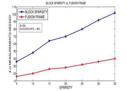
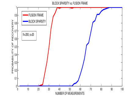
In Fig. 1, we show that the knowledge of the subspaces improves the recovery. To that end, we fix a fusion frame with $N=200$ subspaces in ${\mathbb{R}}^{d}$ with $\lambda_{\mathrm{eff}}\approx 0.6$. Then we vary the sparsity level $s$ from $5$ to $35$, and generate an $s$-sparse vector ${\mathbf{x}}$ in the fusion frame. For each $s$, we vary the number of measurements $m$ and compute empirical recovery rates via the programs

$$\text{(FF)}\ \hat{{\mathbf{x}}}=\text{argmin}_{{\mathbf{x}}\in\mathcal{H}}\|{\mathbf{x}}\|_{2,1}\ \ s.t.\ \ {\bf A_{P}}{\mathbf{x}}={\mathbf{y}},$$ (35)

$$\text{(block)}\ \hat{{\mathbf{x}}}=\text{argmin}_{{\mathbf{x}}}\|{\mathbf{x}}\|_{2,1}\ \ s.t.\ \ {\bf A_{I}}{\mathbf{x}}={\mathbf{y}}.$$ (36)

For the whole period, we leave the vector to be recovered fixed. Repeating this test 100 times with different random $A$ for each choice of parameters $(s,m,N)$ provides an empirical estimate of the success probability. In Fig. 1(a), we plot $m$ which yields at least $96\%$ success rate for each $s$. The difference in two plots is due to the incoherence of the subspaces, i.e., $\lambda{\mathrm{eff}}$. Fig. 1(b) ($d=3$, $k=1$) shows the transition from the unsuccessful regime to the successful regime for the sparsity level $s=20$ for both cases (FF and block sparsity). The transition for the FF case occurs at a smaller value $m$ which reflects Fig. 1(a) in a different way. As a consequence, the assumption ${\mathbf{x}}\in\mathcal{H}$ in (35) allows us to to recover ${\mathbf{x}}$ with far less measurements compared to (36) where such a constraint is not used.

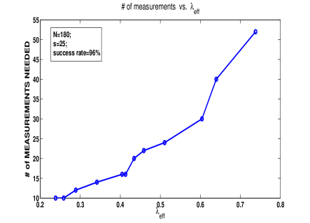
Theorem 3.1 suggests that there is a linear relation between the number of measurements $m$ and the parameter $\lambda_{\mathrm{eff}}$. The experiment depicted in Fig. 2 is designed to reflect this relation. We generate fusion frames with $N=180$ subspaces with various $\lambda_{\mathrm{eff}}$ which is managed by changing $d$ and keeping $k=3$ fixed. Then in each fusion frame, a vector ${\mathbf{x}}$ with sparsity $s=25$ is generated and the number of measurements $m$ that suffices for recovery is determined. The plot yields an almost linear relation in parallel to the theoretical result.

Figure 2: $m$ vs. $\lambda_{\mathrm{eff}}$

Stable case:

In this part, we generate scenarios that allude to the conclusions of Theorems 4.2 and 4.3. In a fusion frame of $N=200$ subspaces, we generate a signal ${\mathbf{x}}$ composed of ${\mathbf{x}}_{S}$, supported on an index set $S$, and a signal ${\mathbf{z}}_{\overline{S}}$ supported on $\overline{S}$. We then normalize ${\mathbf{x}}_{S}$ and ${\mathbf{z}}_{\overline{S}}$ so that $\|{\mathbf{x}}_{S}\|_{2,1}=\|{\mathbf{z}}_{\overline{S}}\|_{2,1}=1$ and produce ${\mathbf{x}}={\mathbf{x}}_{S}+\theta{\mathbf{z}}_{\overline{S}}$ where $\theta\in[0,1]$. Then ${\mathbf{x}}$ is our compressible vector where compressibility is controlled with $\theta$. For measurement, we choose the normalized Gaussian matrix $A\in{\mathbb{R}}^{m\times N}$. We measure ${\mathbf{y}}={\bf A_{P}}{\mathbf{x}}$ and then run the program $(L1)$ and measure the reconstruction error $\|{\mathbf{x}}-\hat{{\mathbf{x}}}\|_{2}$. We repeat this test $20$ times for a fixed ${\mathbf{x}}$ with $\theta=0.12$ in order to obtain an average recovery error for different values of $m$. Fig. 3(a) reports the results of this experiment performed for different fusion frames with various values of $\lambda_{\mathrm{eff}}$ and also for the block sparsity case. The decrease in the reconstruction error with increasing $m$ is natural even though it is not suggested directly by the theoretical results. Indeed, one would expect that increasing the number of measurements would enhance the recovery conditions and yield an improved reconstruction.

For the noisy case, similarly, we generate noisy observations ${\bf A_{P}}{\mathbf{x}}_{S}+\sigma{\mathbf{e}}$, of a sparse signal ${\mathbf{x}}_{S}$ where $\|{\mathbf{x}}_{S}\|_{2}=\|{\mathbf{e}}\|_{2}=1$ and $\sigma=0.06$. Here, all entries of the noise vector ${\mathbf{e}}$ are chosen i.i.d from the standard Gaussian distribution and then properly normalized. We then run the robust $(L1)^{\eta}$ program and measure the reconstruction error $\|{\mathbf{x}}-\hat{{\mathbf{x}}}\|_{2}$. We plot the average of this error vs. the number of measurements in Fig 3(b) for different values of $\lambda_{\mathrm{eff}}$.

(a)

(b)

Figure 3: $\|\hat{{\mathbf{x}}}-{\mathbf{x}}\|_{2}$ vs. ’m’

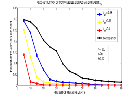
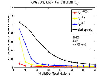
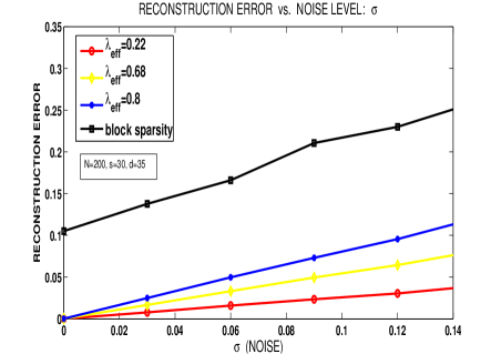
Fig. 4(a) depicts the relation between the reconstruction error and the noise level $\sigma$ for different values of $\lambda_{\mathrm{eff}}$. In this setup, $N=200$, $s=30$ and $m=50$ are fixed, and a sparse vector ${\mathbf{x}}$ in the fusion frame with specific value of $\lambda_{\mathrm{eff}}$ is generated. For each value of $\sigma$ we plot the average reconstruction error. Results manifest the linear relation between $\sigma$ and $\|{\mathbf{x}}-\hat{{\mathbf{x}}}\|_{2}$ given in (34). Again, we obtain a better reconstruction quality when $\lambda_{\mathrm{eff}}$ is smaller.

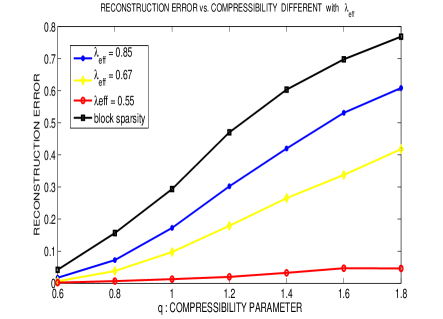
Finally, we examine the relation between compressibility and the reconstruction error using a different model than described earlier. In Fig. 4(b), we plot the results of an experiment in which we generate signals ${\mathbf{x}}$ in a fusion frame with $N=200$, with sorted values of $\|x_{j}\|_{2}$ that decay according to some power law. In particular, for various values of $0<q<1$, we set $\|x_{j}\|_{2}=cj^{-1/q}$ such that $\|{\mathbf{x}}\|_{2}=1$. We then measure ${\mathbf{x}}$ with Gaussian matrices $A$ and compute the average reconstruction errors via $(L1)$ program. Note that the higher the value of $q$, the less compressible the signal is. The results indicate that reconstruction of error decreases when the compressibility of the signal increases as declared in (34). We can also see the improvement in the reconstruction when the subspaces are more incoherent, i.e., they have smaller $\lambda_{\mathrm{eff}}$.

(a)

(b)

Figure 4: $\|\hat{{\mathbf{x}}}-{\mathbf{x}}\|_{2}$ vs. $\sigma$          and             $\|\hat{{\mathbf{x}}}-{\mathbf{x}}\|_{2}$ vs. $q$

6 Appendix

The following theorem is the noncommutative Bernstein inequality due to Tropp, [23, Theorem 1.4].

Theorem 6.1.

(Matrix Bernstein inequality) Let $\{X_{\ell}\}_{\ell=1}^{M}\in{\mathbb{R}}^{d\times d}$ be a sequence of independent random self-adjoint matrices. Suppose that $\mathbb{E}X_{\ell}=0$ and $\|X_{\ell}\|\leq K$ a.s. and put

$$\sigma^{2}:=\left\|\sum_{\ell=1}^{M}\mathbb{E}X_{\ell}^{2}\right\|.$$

Then for all $t\geq 0$,

$$\mathbb{P}\left(\left\|\sum_{\ell=1}^{M}X_{\ell}\right\|\geq t\right)\leq 2d\exp\left(\frac{-t^{2}/2}{\sigma^{2}+Kt/3}\right).$$ (37)

Remark 6.2.

One can improve the tail bound (37) provided the $\{X_{\ell}\}$ are identically distributed and the $\mathbb{E}X_{\ell}^{2}$ are not full rank, say $\mathrm{rank}(\mathbb{E}X_{\ell}^{2})=r<d$. Then (37) can be replaced by

$$\mathbb{P}\left(\left\|\sum_{\ell=1}^{M}X_{\ell}\right\|\geq t\right)\leq 2r\exp\left(\frac{-t^{2}/2}{\sigma^{2}+Kt/3}\right).$$ (38)

Sketch of the proof. We mainly improve [23, Corollary 3.7] under the assumptions above on $X_{\ell}$. By [23, Theorem 3.6], for each $\theta>0$, it holds that

$$\mathbb{P}\left(\lambda_{\max}\left(\sum_{\ell=1}^{M}X_{\ell}\right)\geq t\right)\leq e^{-\theta t}\ {\mathrm{Tr}}\exp\left(\sum_{\ell=1}^{M}\ln\left(\mathbb{E}e^{\theta X_{\ell}}\right)\right),$$

where $\lambda_{\max}$ denotes the largest eigenvalue. Moreover, [23, Lemma 6.7] states that, for $\theta>0$,

$$\mathbb{E}e^{\theta X}\preccurlyeq\exp\left(g(\theta)\mathbb{E}X^{2}\right)$$

for a self-adjoint, centered random matrix $X$, where $g(\theta)=e^{\theta}-\theta-1$. Using this result we obtain

$$\mathbb{P}\left(\lambda_{\max}\left(\sum_{\ell=1}^{M}X_{\ell}\right)\geq t\right) \leq e^{-\theta t}\ {\mathrm{Tr}}\exp\left(g(\theta)\sum_{\ell=1}^{M}\mathbb{E}X_{\ell}^{2}\right)=e^{-\theta t}\ {\mathrm{Tr}}\exp\left(g(\theta)M\mathbb{E}X_{1}^{2}\right)$$

$$\leq e^{-\theta t}r\ \lambda_{\max}\left[\exp\left(g(\theta)M\mathbb{E}X_{1}^{2}\right)\right]=e^{-\theta t}r\ \exp\left(g(\theta)\lambda_{\max}(M\mathbb{E}X_{1}^{2})\right).$$

The first equality above uses that $X_{\ell}$ are identically distributed. The second inequality is valid because, for a positive definite matrix $B$ with rank $r$, we have ${\mathrm{Tr}}B\leq r\lambda_{\max}(B)$ and $\mathrm{rank}(c\ \mathbb{E}X_{\ell}^{2})=\mathrm{rank}\left(\exp(c\ \mathbb{E}X_{\ell}^{2})\right)=r$, for some $c>0$. The rest of the proof proceeds in the same way as the proof of [23, Theorem 1.4].

We also give a rectangular version of the matrix Bernstein inequality as it appears in [23, Theorem 1.6].

Theorem 6.3.

(Matrix Bernstein:rectangular) Let $\{Z_{\ell}\}\in{\mathbb{R}}^{d_{1}\times d_{2}}$ be a finite sequence of independent random matrices. Suppose that $\mathbb{E}Z_{\ell}=0$ and $\|Z_{\ell}\|\leq K$ a.s. and put

$$\sigma^{2}:=\max\left\{\left\|\sum_{\ell}\mathbb{E}(Z_{\ell}Z_{\ell}^{*})\right\|,\left\|\sum_{\ell}\mathbb{E}(Z_{\ell}^{*}Z_{\ell})\right\|\right\}.$$

Then for all $t\geq 0$,

$$\mathbb{P}\left(\left\|\sum_{\ell}Z_{\ell}\right\|\geq t\right)\leq(d_{1}+d_{2})\exp\left(\frac{-t^{2}/2}{\sigma^{2}+Kt/3}\right).$$

The next lemma is a deviation inequality for sums of independent random vectors which is a corollary of Bernstein inequalities for suprema of empirical processes [16, Corollary 8.44]. A similar result can be also found in [18, Theorem 12].

Lemma 6.4.

(Vector Bernstein inequality) Let ${\mathbf{Y}}_{1},{\mathbf{Y}}_{2},\ldots,{\mathbf{Y}}_{M}$ be independent copies of a random vector ${\mathbf{Y}}$ on ${\mathbb{R}}^{n}$ satisfying $\mathbb{E}{\mathbf{Y}}=0$. Assume $\|{\mathbf{Y}}\|_{2}\leq K$. Let

$$Z=\left\|\sum_{\ell=1}^{M}{\mathbf{Y}}_{\ell}\right\|_{2},\ \ \mathbb{E}Z^{2}=M\mathbb{E}\|{\mathbf{Y}}\|_{2}^{2},$$

and

$$\sigma^{2}=\sup_{\|{\mathbf{x}}\|_{2}\leq 1}\mathbb{E}|{\langle}x,{\mathbf{Y}}{\rangle}|^{2}.$$ (39)

Then, for $t>0$,

$$\mathbb{P}(Z\geq\sqrt{\mathbb{E}Z^{2}}+t)\leq\exp\left(-\frac{t^{2}/2}{M\sigma^{2}+2K\sqrt{\mathbb{E}Z^{2}}+tK/3}\right).$$ (40)

Remark 6.5.

The so-called weak variance $\sigma^{2}$ in (39) can be estimated by

$$\sigma^{2}=\sup_{\|{\mathbf{x}}\|_{2}\leq 1}\mathbb{E}|{\langle}x,{\mathbf{Y}}{\rangle}|^{2}\leq\mathbb{E}\sup_{\|{\mathbf{x}}\|_{2}\leq 1}|{\langle}x,{\mathbf{Y}}{\rangle}|^{2}=\mathbb{E}\|{\mathbf{Y}}\|_{2}^{2}.$$

References

- [1] U. Ayaz. Sparse Recovery with Fusion Frames. 2014. Ph.D. thesis. Hausdorff Center for Mathematics, University of Bonn.
- [2] U. Ayaz, S. Dirksen, and H. Rauhut. Uniform recovery of fusion frame structured sparse signals. (Submitted).
- [3] U. Ayaz and H. Rauhut. Nonuniform sparse recovery with subgaussian matrices. ETNA, to appear.
- [4] P. E. Bjørstad and J. Mandel. On the spectra of sums of orthogonal projections with applications to parallel computing. BIT, 31(1):76–88, Mar. 1991.
- [5] B. G. Bodmann. Optimal linear transmission by loss-sensitive packet encoding. Appl. Comput. Harmon. Anal., 22(3):274–285, 2007.
- [6] P. Boufounos, G. Kutyniok, and H. Rauhut. Sparse recovery from combined fusion frame measurements. IEEE Trans. Inform. Theory, 57(6):3864–3876, 2011.
- [7] E. Candès, J. Romberg, and T. Tao. Robust uncertainty principles: exact signal reconstruction from highly incomplete frequency information. IEEE Trans. Inf. Theory, 52(2):489–509, 2006.
- [8] E. Candès and T. Tao. Near optimal signal recovery from random projections: universal encoding strategies? IEEE Trans. Inf. Theory, 52(12):5406–5425, 2006.
- [9] P. Casazza and G. Kutyniok. Fusion Frames. Applied and Numerical Harmonic Analysis. Boston, MA: Birkhäuser. xvi, 2013.
- [10] P. G. Casazza and G. Kutyniok. Frames of subspaces. in Wavelets, Frames and Operator Theory, pages 87–113, 2004.
- [11] P. G. Casazza, G. Kutyniok, S. Li, and C. J. Rozell. Modeling sensor networks with fusion frames. In Wavelets Xll, Special Session on Finite-Dimensional Frames, Time-Frequency Analysis, and Applications, volume 6701, page 11, 2007.
- [12] V. Chandrasekaran, B. Recht, P. A. Parrilo, and A. S. Willsky. The convex geometry of linear inverse problems. Foundations of Computational Mathematics, 12(6), 2012.
- [13] D. Donoho. Compressed sensing. IEEE Trans. Inform. Theory, 52(4):1289–1306, 2006.
- [14] Y. C. Eldar and H. Bölcskei. Block-sparsity: Coherence and efficient recovery. In ICASSP, pages 2885–2888. IEEE, 2009.
- [15] M. Fornasier and H. Rauhut. Recovery algorithms for vector valued data with joint sparsity constraints. SIAM J. Numer. Anal., 46(2):577–613, 2008.
- [16] S. Foucart and H. Rauhut. A mathematical introduction to compressive sensing. Applied and Numerical Harmonic Analysis. Birkhäuser, 2013.
- [17] J.-J. Fuchs. On sparse representations in arbitrary redundant bases. IEEE Trans. Inf. Th, page 1344, 2004.
- [18] D. Gross. Recovering low-rank matrices from few coefficients in any basis. IEEE Transactions on Information Theory, 57(3):1548–1566, 2011.
- [19] G. Kutyniok, A. Pezeshki, R. Calderbank, and T. Liu. Robust dimension reduction, fusion frames, and Grassmannian packings. Appl. Comput. Harmon. Anal., 26(1):64–76, 2009.
- [20] P. Oswald. Frames and space splittings in Hilbert spaces. Technical report, 1997.
- [21] N. S. Rao, B. Recht, and R. D. Nowak. Universal measurement bounds for structured sparse signal recovery. Jour. of Mach. Learn. Res. - Proc. Track, 22:942–950, 2012.
- [22] J. Tropp. Recovery of short, complex linear combinations via minimization. IEEE Trans. Inf. Theory, 51(4):1568–1570, 2005.
- [23] J. A. Tropp. User-friendly tail bounds for sums of random matrices. Found. of Comp. Math., 12(4):389–434, 2012.
- [24] E. van den Berg and M. P. Friedlander. SPGL1: A solver for large-scale sparse reconstruction, June 2007. http://www.cs.ubc.ca/labs/scl/spgl1.
- [25] E. van den Berg and M. P. Friedlander. Probing the pareto frontier for basis pursuit solutions. SIAM Journ. on Scien. Comp., 31(2):890–912, 2008.