The VLT-FLAMES Tarantula Survey

Previous analyses of the spectra of OB-type stars in the Magellanic Clouds have identified targets with low projected rotational velocities and relatively high nitrogen abundances; the evolutionary status of these objects remains unclear. The VLT-FLAMES Tarantula Survey obtained spectroscopy for over 800 early-type stars in 30 Doradus of which 434 stars were classified as B-type. We have estimated atmospheric parameters and nitrogen abundances using tlusty model atmospheres for 54 B-type targets that appear to be single, have projected rotational velocities, $v_{\rm{e}}\sin i$ $\leq$ 80 km s^-1and were not classified as supergiants. In addition, nitrogen abundances for 34 similar stars observed in a previous FLAMES survey of the Large Magellanic Cloud have been re-evaluated.

For both samples, approximately 75-80% of the targets have nitrogen enhancements of less than 0.3 dex, consistent with them having experienced only small amounts of mixing. However, stars with low projected rotational velocities, $v_{\rm{e}}\sin i$ $\leq$ 40 km s^-1 and significant nitrogen enrichments are found in both our samples and simulations imply that these cannot all be rapidly rotating objects observed near pole-on. For example, adopting an enhancement threshold of 0.6 dex, we observed five and four stars in our VFTS and previous FLAMES survey samples, yet stellar evolution models with rotation predict only 1.25$\pm$1.11 and 0.26$\pm$0.51 based on our sample sizes and random stellar viewing inclinations. The excess of such objects is estimated to be 20-30% of all stars with current rotational velocities of less than 40 km s^-1. This would correspond to $\sim$2-4% of the total non-supergiant single B-type sample. Given the relatively large nitrogen enhancement adopted, these estimates constitute lower limits for stars that appear inconsistent with current grids of stellar evolutionary models. Including targets with smaller nitrogen enhancements of greater than 0.2 dex implies larger percentages of targets that are inconsistent with current evolutionary models, viz. $\sim$70% of the stars with rotational velocities less than 40 km s^-1and $\sim$6-8% of the total single stellar population. We consider possible explanations of which the most promising would appear to be breaking due to magnetic fields or stellar mergers with subsequent magnetic braking.

1 Introduction

The evolution of massive stars during their hydrogen core burning phase has been modelled for over sixty years with early studies by, for example, Tayler (1954, 1956); Kushwaha (1957); Schwarzschild & Härm (1958); Henyey et al. (1959); Hoyle (1960). These initial models lead to a better understanding of, for example, the observational Hertzsprung-Russell diagram for young clusters (Henyey et al. 1959) and the dynamical ages inferred for young associations (Hoyle 1960). Subsequently there have been major advances in the physical assumptions adopted in such models, including the effects of stellar rotation (Maeder 1987), mass loss (particularly important in more luminous stars and metal-rich environments; Chiosi & Maeder 1986; Puls et al. 2008; Mokiem et al. 2007) and magnetic fields (Donati & Landstreet 2009; Petermann et al. 2015). Recent reviews of these developments include Maeder (2009) and Langer (2012).

Unlike late-type stars, where stellar rotation velocities are generally small (see, for example, Gray 2005, 2016, 2017, and references therein), rotation is an important phenomenon affecting both the observational and theoretical understanding of early-type stars. Important observational studies of early-type stellar rotation in our Galaxy include Slettebak (1949), Conti & Ebbets (1977), Penny (1996), Howarth et al. (1997), Abt et al. (2002), Huang et al. (2010) and Simón-Díaz & Herrero (2014). There have also been extensive investigations for the Magellanic Clouds using ESO large programmes, viz. Martayan et al. (2006, 2007, and references therein), Evans et al. (2005, 2006) and Hunter et al. (2008b). More recently as part of the VLT-Flames Tarantula Survey (Evans et al. 2011), rotation in both apparently single (Ramírez-Agudelo et al. 2013; Dufton et al. 2013) and binary (Ramírez-Agudelo et al. 2015) early-type stars has been investigated. These studies all show that early-type stars cover the whole range of rotational velocities up to the critical velocity at which the centrifugal force balances the stellar gravity at the equator (Struve 1931; Townsend et al. 2004).

These observational studies have led to rotation being incorporated into stellar evolutionary models (see, for example, Maeder 1987; Heger & Langer 2000; Hirschi et al. 2004; Frischknecht et al. 2010), leading to large grids of rotating evolutionary models for different metallicity regimes (Brott et al. 2011a; Ekström et al. 2012; Georgy et al. 2013a, b). Such models have resulted in a better understanding of the evolution of massive stars, including main-sequence life times (see, for instance Meynet & Maeder 2000; Brott et al. 2011a; Ekström et al. 2012) and the possibility of chemically homogeneous evolution (Maeder 1980; Maeder et al. 2012; Szécsi et al. 2015), that in low-metallicity environments could lead to gamma-ray bursts (Yoon & Langer 2005; Yoon et al. 2006; Woosley & Heger 2006). However there remain outstanding issues in the evolution of massive single and binary stars (Meynet et al. 2017). For example, nitrogen enhanced early-type stars with low projected rotational velocities that may not be the result of rotational mixing have been identified by Hunter et al. (2008a), Rivero González et al. (2012), and Grin et al. (2017). The nature of these stars have discussed previously by, for example, Brott et al. (2011b), Maeder et al. (2014), and Aerts et al. (2014). Definitive conclusions have been hampered both by observational and theoretical uncertainties and by the possibility of other evolutionary scenarios (see Grin et al. 2017, for a recent detailed discussion).

Here we discuss the apparently single B-type stars with low projected rotational velocity found in the VLT-Flames Tarantula Survey (Evans et al. 2011, hereafter VFTS). These complement the analysis of the corresponding binary stars from the same survey by Garland et al. (2017). We also reassess the results of Hunter et al. (2007, 2008a) and Trundle et al. (2007a) from a previous spectroscopic survey (Evans et al. 2006). In particular we investigate whether there is an excess of nitrogen enhanced stars with low projected velocities and attempt to quantify any such excess. We then use these results to constrain the evolutionary pathways that may have produced these stars.

2 Observations

The VFTS spectroscopy was obtained using the MEDUSA and ARGOS modes of the FLAMES instrument (Pasquini et al. 2002) on the ESO Very Large Telescope. The former uses fibres to simultaneously ‘feed’ the light from over 130 stellar targets or sky positions to the Giraffe spectrograph. Nine fibre configurations (designated fields ‘A’ to ‘I’ with near identical field centres) were observed in the 30 Doradus region, sampling the different clusters and the local field population. Spectroscopy of more than 800 stellar targets was obtained and approximately half of these were subsequently spectrally classified by Evans et al. (2015) as B-type. The young massive cluster at the core of 30 Doradus, R136, was too densely populated for the MEDUSA fibres, and was therefore observed with the ARGUS integral field unit (with the core remaining unresolved even in these observations). Details of target selection, observations, and initial data reduction have been given in Evans et al. (2011), where target co-ordinates are also provided.

The analysis presented here employed the FLAMES–MEDUSA observations that were obtained with two of the standard Giraffe settings, viz. LR02 (wavelength range from 3960 to 4564 Å at a spectral resolving power of R$\sim$7 000) and LR03 (4499-5071 Å, R$\sim$8 500). The targets identified as B-type (excluding a small number with low quality spectra) have been analysed using a cross-correlation technique to identify radial velocity variables (Dunstall et al. 2015). For approximately 300 stars, which showed no evidence of significant radial velocity variations, projected rotational velocities, $v_{\rm{e}}\sin i$, have been estimated by Dufton et al. (2013) and Garland et al. (2017).

In principle, a quantitative analysis of all these apparently single stars, including those with large projected rotational velocities, would have been possible. However, the moderate signal-to-noise ratios (S/N) of our spectroscopy would lead to the atmospheric parameters (especially the effective temperature and microturbulence – see Sect. 4.2 and 4.4) being poorly constrained for the broader lined targets. In turn this would lead to nitrogen abundance estimates that had little diagnostic value. Hence for the purposes of this paper we have limited our sample to the subset with relatively small projected rotational velocities. This is consistent with the approach adopted by Garland et al. (2017) in their analysis of the corresponding narrow lined B-type VFTS binaries.

Hence our targets were those classified as B-type with a luminosity class III to V, which showed no evidence of significant radial velocity variations and had an estimated $v_{\rm{e}}\sin i$ $\leq$80 km s^-1; the B-type supergiants (luminosity classes I to II) have been discussed previously by McEvoy et al. (2015). Stars with an uncertain O9 or B0 classification have not been included. Additionally the spectrum of VFTS 469 had been identified in Paper I as suffering some cross contamination from a brighter O-type star in an adjacent fibre. Another of our targets, VFTS 167, may also suffer such contamination as the He ii line at 4686 Å shows broad emission. We retain these two stars in our sample but discuss the reliability of their analyses in Sect. 6.2. Some of our apparently single stellar sample will almost certainly have a companion. In particular, as discussed by Dunstall et al. (2015), low mass companions or binaries in wide orbits may not have been identified.

Table 1 summarises the spectral types (Evans et al. 2015) and typical S/N (rounded to the nearest multiple of five) in the LR02 spectral region. The latter were estimated from the wavelength region, 4200-4250 Å, which should not contain strong absorption lines. However particularly for the higher estimates, these should be considered as lower limits as they could be affected by weak lines. S/N for the LR03 region were normally similar or slightly smaller (see, for example, McEvoy et al. 2015, for a comparison of the ratios in the two spectral region). Also listed are the estimated projected rotational velocity, $v_{\rm{e}}\sin i$ (Dufton et al. 2013; Garland et al. 2017), the mean radial velocity, $v_{\rm{r}}$ (Evans et al. 2015), and the range, $\Delta v_{\rm{r}}$, in radial velocity estimates (Dunstall et al. 2015). The moderate spectral resolving power led to estimates of the projected rotational velocity for stars with $v_{\rm{e}}\sin i$ $\leq$ 40 km s^-1 being poorly constrained and hence approximately half the sample have been assigned to a bin with $0\leq$ $v_{\rm{e}}\sin i$ $\leq 40$ km s^-1.

Luminosities have also been estimated for our targets using a similar methodology to that adopted by Garland et al. (2017). Interstellar extinctions were estimated from the observed $B-V$ colours provided in Evans et al. (2011), together with the intrinsic colour–spectral-type calibration of Wegner (1994) and $R_{V}=3.5$ (Doran et al. 2013). Bolometric corrections were obtained from LMC-metallicity tlusty models (Lanz & Hubeny 2007) and together with an adopted LMC distance modulus of 18$\aas@@fstack{m}$49 (Pietrzyński et al. 2013), the stellar luminosity were estimated. Table 1 lists these estimates (hereafter designated as ‘observed luminosities’) apart from that for VFTS 835 for which no reliable photometry was available. The main sources of uncertainty in these luminosity estimates will arise from the bolometric correction and the extinction. We estimate that these will typically contribute an error of $\pm 0^{\mathrm{m}}$​​.5 in the absolute magnitude corresponding to $\pm$0.2 dex in the luminosity. We note these error estimates are consistent with the luminosities deduced from evolutionary models discussed in Sect. 6.6.1.

For both the LR02 and LR03 spectroscopy , all useable exposures were combined using either a median or weighted $\sigma$-clipping algorithm. The final spectra from the different methods were normally indistinguishable. The full wavelength range for each wavelength setting could usually be normalised using a single, low-order polynomial. However, for some features (e.g. the Balmer series), the combined spectra around individual (or groups of) lines were normalised.

In the model atmosphere analysis, equivalent widths were generally used for the narrower metal lines, with profiles being considered for the broader H i and He ii lines. For the former, Gaussian profiles (and a low order polynomial to represent the continuum) were fitted to the observed spectra leading to formal errors in the equivalent width estimates of typically 10%. The fits were generally convincing which is consistent with the intrinsic and instrumental broadening being major contributors to these narrow lined spectra. Tests using rotationally broadened profiles yielded equivalent width estimates in good agreement with those using Gaussian profiles – differences were normally less than 10% but the fits were generally less convincing.

For some spectra, lines due to important diagnostic species (e.g. Si ii, Si iv and N ii) could not be observed; in these cases we have set upper limits on the equivalent widths. Our approach was to measure the equivalent width of the weakest metal line or lines that were observable in the VFTS spectra of narrow lined stars. These were then rounded to the nearest 5 mÅ  and plotted against the S/N of the spectra as shown in Fig. 1. The equivalent widths decrease with increasing S/N as would be expected and there also seems to be no significant difference for stars with 0 $<$ $v_{\rm{e}}\sin i$ $\leq$40 km s^-1 and those with 40 $<$ $v_{\rm{e}}\sin i$ $\leq$ 80 km s^-1. The upper limit for an equivalent width at a given S/N probably lies at or near the lower envelope of this plot. However we have taken a more cautious approach by fitting a low order polynomial to these results and using this to estimate upper limits to equivalent widths of unseen lines. We emphasise that this will lead to conservative estimates both for the upper limits of equivalent widths and for the corresponding element abundances.

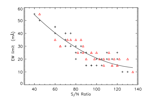
Figure 1: Estimated equivalent width limits (in mÅ) plotted against the S/N of the VFTS spectra. Crosses and triangles represent stars with $v_{\rm{e}}\sin i$ $\leq$ 40 km s^-1 and 40 $<$ $v_{\rm{e}}\sin i$ $\leq$ 80 km s^-1 respectively. A quadratic linear least squares fit for all the estimates is also shown.

The VFTS data have been supplemented by those from a previous FLAMES/VLT survey (Evans et al. 2005, hereafter the FLAMES-I survey). Spectral classification by Evans et al. (2006) identified 49 B-type stars that also had $v_{\rm{e}}\sin i$ $\leq$ 80 km s^-1 (Hunter et al. 2008b). Fourteen of these were characterised as binaries (Evans et al. 2006), either SB2 (on the basis of their spectra) or SB1 (on the basis of radial velocity variations between epochs). These targets were discussed by Garland et al. (2017) and will not be considered further. For the apparently single stars, atmospheric parameters previously estimated from this FLAMES-I spectroscopy (Hunter et al. 2007, 2008a, 2009; Trundle et al. 2007b) have been adopted. However we have re-reduced the spectroscopy for the wavelength region incorporating the N ii line at 3995 Å, using the methods outlined above. This should provide a better data product than the simple co-adding of exposures that was under taken in the original analyses. Comparison of spectra from the two reductions confirmed this (although in many cases the improvement was small).

3 Binarity criteria

Dunstall et al. (2015) adopted two criteria for the identification of binary systems. Firstly the difference between two estimates of the radial velocity had to be greater than four times the estimated uncertainty and secondly this difference had to be greater than 16 km s^-1; this threshold was chosen so as to limit false positives due to for example pulsations that are likely to be significant particularly in supergiants (Simón-Díaz et al. 2010; Taylor et al. 2014; Simón-Díaz et al. 2017a). In Table 1, the ranges ($\Delta v_{\rm{r}}$) of radial velocities of six targets fulfil the latter (but not the former) criteria. As discussed by Dunstall et al. (2015) a significant fraction of binaries may not have been identified and these six targets could therefore be binaries. Four of these targets (VFTS 010, 625, 712, 772) were not analysed due to the relatively low S/N of their spectroscopy (see Sect. 4), which probably contributed their relatively large values of $\Delta v_{\rm{r}}$.

For the other two targets, we have re-evaluated the spectroscopy as follow:

VFTS 313: Dunstall et al. (2015) obtained radial velocity estimates only from the He i diffuse lines at 4026 and 4387 Å, which may have contributed to the relatively large value of $\Delta v_{\rm{r}}$ $\sim$ 18 km s^-1. There was considerable scatter between estimates found for exposures obtained at a given epoch, especially the first epoch when six consecutive exposures were available. Given the high cadence of these observations, these variations are unlikely to be real and probably reflect uncertainties in the individual measurements. The best observed intrinsically narrow feature in the LR02 spectra was the Si iv and O ii close blend (separation of 0.60 Å) at 4089 Å. Radial velocity estimates were possible for eleven out the twelve LR02 exposures (the other exposure was affected by a cosmic ray event) from fitting a Gaussian profile to this blend. The estimates ranged from 270-282 km s^-1 with a mean value of 275.1$\pm$4.4 km s^-1 (assuming that the Si iv feature dominates the blend).

VFTS 835: Dunstall et al. (2015) obtained radial velocity estimates only from the He i diffuse lines at 4026, 4387 and 4471 Å, which may again have contributed to the relatively large value of $\Delta v_{\rm{r}}$ $\sim$ 18 km s^-1. As for VFTS 313, there was again considerable scatter between estimates found for exposures within a given epoch. Unfortunately the metal lines were broadened by stellar rotation, which precluded their use for estimating reliable radial velocities in the single exposures, which had relatively low S/N.  

Hence we find no convincing evidence for binarity in either of these targets and have retained them in our apparently single star sample.

Table 1: VFTS B-type targets with a luminosity class V to III (Evans et al. 2015), which show no evidence of significant radial velocity variations (Dunstall et al. 2015; Evans et al. 2015) and have a $v_{\rm{e}}\sin i$ $\leq$ 80 km s^-1 (Dufton et al. 2013; Garland et al. 2017). The mean radial velocities, $v_{\rm{r}}$ are from Evans et al. (2015) and the ranges, $\Delta v_{\rm{r}}$, in radial velocity estimates are from Dunstall et al. (2015) with all velocities having units of km s^-1. Further detail on the targets including their co-ordinates can be found in Evans et al. (2011). The estimates of the S/N for the LR02 region have been rounded to the nearest multiple of five, whilst luminosities, L, were estimated as discussed in Sect. 2.

VFTS	ST	S/N	$v_{\rm{e}}\sin i$	$v_{\rm{r}}$	$\Delta v_{\rm{r}}$	$\log$ L/ $\rm{L}_{\odot}$
010	B2 V	40	$\leq$40	287	25	3.87
024	B0.2 III-II	100	58	286	10	4.80
029	B1 V	80	$\leq$40	286	10	3.95
044	B2 V	80	65	288	7	3.79
050	B0 V	60	$\leq$40	283	3	4.35
052	B0.2 III-II	145	48	280	4	4.77
053	B1 III	125	$\leq$40	276	3	4.56
075	B1 V	65	70	297	3	3.94
095	B0.2 V	100	$\leq$40	294	4	4.36
111	B2 III	215	80	272	2	4.56
119	B0.7 V	60	$\leq$40	276	11	4.27
121	B1 IV	115	$\leq$40	284	3	4.31
124	B2.5 III	75	$\leq$40	289	6	4.04
126	B1 V	80	$\leq$40	254	3	3.86
152	B2 IIIe	130	47	274	4	4.65
167	B1 V	110	$\leq$40	286	14	4.26
170	B1 IV	120	$\leq$40	279	1	4.41
183	B0 IV-III	70	$\leq$40	256	2	4.66
202	B2 V	120	49	277	7	4.25
209	B1 V	80	$\leq$40	273	14	4.06
214	B0 IV-III	80	$\leq$40	276	4	4.78
237	B1-1.5 V-IVe	110	79	288	10	4.35
241	B0 V-IV	75	69	268	16	4.14
242	B0 V-IV	60	$\leq$40	216	8	4.17
273	B2.5 V	70	$\leq$40	254	4	3.78
284	B1 V	80	$\leq$40	273	15	3.91
297	B1.5 V	80	47	252	9	4.01
308	B2 V	160	74	263	3	4.17
313	B0 V-IV	110	56	270	18	4.41
331	B1.5 V	100	64	279	3	3.84
347	B0 V	95	$\leq$40	268	4	4.19
353	B2 V-III	90	63	292	7	4.02
363	B0.2 III-II	225	50	264	7	4.64
384	B0 V-III	65	46	266	6	4.79
469	B0 V	100	$\leq$40	276	3	4.41
478	B0.7 V-III	85	64	273	13	4.41
504	B0.7 V	95	60	251	13	5.06
540	B0 V	85	54	247	12	4.55
553	B1 V	85	50	277	7	3.96
572	B1 V	115	68	249	12	4.33
593	B2.5 V	70	$\leq$40	292	7	3.82
616	B0.5: V	100	$\leq$40	227	8	4.29
623	B0.2 V	110	$\leq$40	269	4	4.57
625	B1.5 V	65	64	310	41	4.00
650	B1.5 V	60	$\leq$40	287	6	3.68
666	B0.5 V	95	$\leq$40	255	3	4.07
668	B0.7 V	90	$\leq$40	270	5	4.21
673	B1 V	80	$\leq$40	278	2	3.92
692	B0.2 V	95	$\leq$40	271	3	4.42
707	B0.5 V	145	$\leq$40	275	10	4.61
712	B1 V	120	67	255	17	4.52
725	B0.7 III	120	$\leq$40	286	5	4.39

Table 1: (continued.)

VFTS	ST	S/N	$v_{\rm{e}}\sin i$	$v_{\rm{r}}$	$\Delta v_{\rm{r}}$	$\log$ L/ $\rm{L}_{\odot}$
			km s-1
727	B3 III	70	76	272	7	3.84
740	B0.7 III	45	$\leq$40	268	13	4.48
748	B0.7 V	85	62	261	11	4.23
772	B3-5 V-III	70	61	254	17	3.41
801	B1.5 V	75	$\leq$40	278	7	4.13
835	B1 Ve	80	47	253	18	-
851	B2 III	120	$\leq$40	229	2	3.97
860	B1.5 V	75	60	253	3	4.12
864	B1.5 V	70	$\leq$40	278	13	3.94
868	B2 V	60	$\leq$40	262	8	4.25
872	B0 V-IV	100	77	287	6	4.30
879	B3 V-III	40	$\leq$40	276	16	3.77
881	B0.5 III	80	$\leq$40	283	3	4.28
885	B1.5 V	95	69	264	9	4.26
886	B1 V	65	$\leq$40	258	14	3.89

4 Atmospheric parameters

4.1 Methodology

We have employed model-atmosphere grids calculated with the tlusty and synspec codes (Hubeny 1988; Hubeny & Lanz 1995; Hubeny et al. 1998; Lanz & Hubeny 2007). They cover a range of effective temperature, 10 000K $\leq$$T_{\mathrm{eff}}$ $\leq$35 000K in steps of typically 1 500K. Logarithmic gravities (in cm s^-2) range from 4.5 dex down to the Eddington limit in steps of 0.25 dex, and microturbulences are from 0-30 km s^-1 in steps of 5 km s^-1. As discussed in Ryans et al. (2003) and Dufton et al. (2005), equivalent widths and line profiles interpolated within these grids are in good agreement with those calculated explicitly at the relevant atmospheric parameters.

These non-LTE codes adopt the ‘classical’ stationary model atmosphere assumptions, that is plane-parallel geometry, hydrostatic equilibrium, and the optical spectrum is unaffected by winds. As the targets considered here have luminosity classes V to III, such an approach should provide reliable results. The grids assumed a normal helium to hydrogen ratio (0.1 by number of atoms) and the validity of this is discussed in Sect.  6.2. Grids have been calculated for a range of metallicities with that for an LMC metallicity being used here. As discussed by Dufton et al. (2005), the atmospheric structure depends principally on the iron abundance with a value of 7.2 dex having been adopted for the LMC; this is consistent with estimates of the current iron abundance for this galaxy (see, for example, Carrera et al. 2008; Palma et al. 2015; Lemasle et al. 2017). However we note that, although tests using the Galactic (7.5 dex) or SMC (6.9 dex) grids led to small changes in the atmospheric parameters (primarily to compensate for the different amounts of line blanketing), changes in element abundances estimates were typically less than 0.05 dex. Further information on the tlusty grids are provided in Ryans et al. (2003) and Dufton et al. (2005)

Thirteen of the targets listed in Table 1 have not been analysed (VFTS 010, 044, 152, 504, 593, 625, 712, 727, 772, 801, 879, 885, 886). Most of these stars had spectroscopy with relatively low S/N, whilst several also suffered from strong contamination by nebular emission. The former precluded the estimation of the effective temperature from the silicon ionisation equilibrium, whilst the latter impacted on the estimation of the surface gravity. In turn this led to unreliable atmospheric parameters, and hence any estimates of (or limits on) the nitrogen abundances would have had limited physical significance.

The four characteristic parameters of a static stellar atmosphere, (effective temperature, surface gravity, microturbulence and metal abundances) are inter-dependant and so an iterative process was used to estimate these values.

4.2 Effective Temperature

Effective temperatures ($T_{\mathrm{eff}}$ ) were principally determined from the silicon ionisation balance. For the hotter targets, the Si iii (4552, 4567, 4574 Å) and Si iv (4089, 4116 Å) spectra were used while for the cooler targets, the Si iii and Si ii (4128, 4130 Å) spectra were considered. The estimates of the microturbulence from the absolute silicon abundance (method 2 in Sect. 4.4) were adopted. In some cases it was not possible to measure the strength of either the Si ii or Si iv spectrum. For these targets, upper limits were set on their equivalent widths, allowing limits to the effective temperatures to be estimated, (see, for example, Hunter et al. 2007, for more details). These normally yielded a range of effective temperatures of less than 2000K, with the midpoint being adopted.

For the hotter stars, independent estimates were obtained from the He ii spectrum (at 4541Å and 4686Å). There was good agreement between the estimates obtained using the two methods, with differences typically being 500-1 000 K as can be seen from Table 2. A conservative stochastic uncertainty of $\pm$1 000 K has been adopted for the adopted effective temperature estimates listed in Table 3.

Table 2: Estimates of the atmospheric parameters for the VFTS sample. Effective temperatures ($T_{\mathrm{eff}}$ ) are from the silicon ionisation balance (Si) or He ii profiles – those constrained by the absence of the Si ii and Si iv spectra are marked with an asterisk. Microturbulences ($v_{\rm{t}}$) are from the relative strengths of the Si iii triplet (method 1) or the absolute silicon abundance (method 2). Stars for which no solution could be found for the micrtoturbulence are identified by daggers.

VFTS	$T_{\mathrm{eff}}$ (K)			$\log g$	$v_{\rm{t}}$ (km s-1)
	Si	4686Å	4541Å	(cm s-2)	(1)	(2)
024	27500	27000	-	3.3	9	​​​10
029	27000	27000	-	4.1	0	4
050	30500	30500	30000	4.0	0	1
052	27500	27000	-	3.4	​​​11	9
053	24500	-	-	3.5	0	4
075	23500∗	-	-	3.8	0	6
095	31000	30000	-	4.4	0	0†
111	22000∗	-	-	3.3	-	0†
119	27500	27000	-	4.2	0†	0†
121	24000	-	-	3.6	1	0
124	20000	-	-	3.4	-	1
126	23500∗	-	-	3.8	0	2
167	27000	-	-	4.0	0	0
170	23000	-	-	3.5	0	0
183	29000	28500	28500	3.5	5	4
202	23500∗	-	-	3.9	1	0
209	27500	26500	-	4.3	0	0
214	29000	29500	29500	3.6	3	3
237	23000	-	-	3.6	0	2
241	-	30500	30500	4.0	-	0
242	29500	29000	29000	3.9	0	0
273	19000	-	-	3.8	-	5
284	23500∗	-	-	3.9	1	0
297	23500∗	-	-	3.6	2	0†
308	23500∗	-	-	3.8	3	0†
313	27500	30000	29000	3.8	0	0†
331	24000∗	-	-	3.9	4	2
347	30500	29500	30000	4.0	0	0
353	23000∗	-	-	3.5	-	2
363	27000	27500	26500	3.3	​​​10	9
384	28000	27500	27500	3.3	​​​12	9
469	29500	-	29000	3.5	0	1
478	25500	25500	-	3.6	8	6
540	30000	30000	30000	4.0	5	1
553	24500	-	-	3.8	0	1
572	25500	-	-	4.0	0	2
616	29000	27500	-	4.4	0	0†
623	28500	28500	29000	3.9	1	3
650	23500∗	-	-	3.8	5	7
666	28500	28000	-	4.0	0	0
668	25000	25500	-	3.8	0	2
673	25500	-	-	4.0	0	1
692	29500	29500	29500	3.9	0	2
707	27500	27000	-	4.0	0	0
725	23500	24000	-	3.5	4	6
740	22500	-	-	3.4	9	11
748	29000	27500	-	4.1	4	5
835	23500∗	-	-	3.8	0	2
851	20500	-	-	3.4	-	0
860	23500∗	-	-	3.8	0	6
864	27000	-	-	4.1	0	1
868	23000∗	-	-	3.6	6	6
872	31000	30500	30500	4.1	0	1
881	26500	27000	-	3.8	4	6

4.3 Surface Gravity

The logarithmic surface gravity ($\log g$ ; cm s^-2) for each star was estimated by comparing theoretical and observed profiles of the hydrogen Balmer lines, H$\gamma$ and H$\delta$. H$\alpha$ and H$\beta$ were not considered as they were more affected by the nebular emission. Automated procedures were developed to fit the theoretical spectra to the observed lines, with regions of best fit displayed by contour maps of $\log g$ against $T_{\mathrm{eff}}$ . Using the effective temperatures deduced by the methods outlined above, the gravity could be estimated. Estimates derived from the two hydrogen lines normally agreed to 0.1 dex and their averages are listed in Table 2. Other uncertainties may arise from, for example, errors in the normalisation of the observed spectra and uncertainty in the line broadening theory. For the former, tests using different continuum windows implied that errors in the continuum should be less than 1%, translating into a typical error in the logarithmic gravity of less than 0.1 dex. The uncertainty due to the latter is difficult to assess and would probably mainfest itself in a systematic error in the gravity estimates. Hence, taking these factors into consideration, a conservative uncertainty of $\pm$0.2 dex has been adopted for the gravity estimates listed in Table 3.

4.4 Microturbulence

Microturbulent velocities ($v_{\rm{t}}$) have been introduced to reconcile abundance estimates from lines of different strengths for a given ionic species (see, for example, Gray 2005). We have used the Si iii triplet (4552, 4567 and 4574 Å) because it is observed in almost all of our spectra and all of the lines come from the same multiplet, thereby minimising the effects of errors in the absolute oscillator strengths and non-LTE effects. This approach (method 1 in Table 2) has been used previously in both the Tarantula survey (McEvoy et al. 2015) and a previous FLAMES-I survey (Dufton et al. 2005; Hunter et al. 2007) and these authors noted its sensitivity to errors in the equivalent width measurements of the Si iii lines, especially when the lines lie close to the linear part of the curve of growth. Indeed this was the case for four of our cooler targets where the observations (assuming typical errors of 10% in the equivalent width estimates) did not constrain the microturbulence. The method also requires that all three lines be reliably observed, which was not always the case with the current dataset. Because of these issues, the microturbulence was also derived by requiring that the silicon abundance should be consistent with the LMC’s metallicity (method 2 in Table 2). We adopt a value of 7.20 dex as found by Hunter et al. (2007) using similar theoretical methods and observational data to those here; we note that this is -0.31 dex lower than the solar value given by Asplund et al. (2009).

Seven targets had a maximum silicon abundance (i.e. for $v_{\rm{t}}$= 0 km s^-1) below the adopted LMC value and these are identified in Table 2. These targets have a mean silicon abundance of 6.96$\pm$0.08 dex. Additionally for VFTS 119 it was not possible to remove the variation of silicon abundance estimate with line strength. Both McEvoy et al. (2015) and Hunter et al. (2007) found similar effects for some of their targets, with the latter discussing the possible explanations in some detail. In these instances, we have adopted the best estimate, that is zero microturbulence. For other targets an estimated uncertainty of $\pm$10% in the equivalent widths, translated to variations of typically 3 km s^-1  for both methodologies.

This uncertainty is consistent with the differences between the estimates using the two methodologies. The mean difference (method 1 minus method 2) of the microturbulence is -0.6$\pm$2.0 km s^-1. Only in two cases do they differ by more than 5 km s^-1 and then the estimates from the relative strength of the Si iii multiplet appear inconsistent with those found for other stars with similar gravities. However, a conservative stochastic uncertainty of $\pm$5 km s^-1 has been adopted for the values listed in Table 3

Table 3: Estimates of the atmospheric parameters and element abundances for the VFTS B-type stars.

VFTS	$v_{\rm{e}}\sin i$	$T_{\mathrm{eff}}$	$\log g$	$v_{\rm{t}}$	$\epsilon_{\rm{Mg}}$	$\epsilon_{\rm{N}}$
	(km s-1)	(K)	(cm s-2)	(km s-1)	dex	dex
024	58	27500	3.3	10	6.92	$\leq$7.4
029	$\leq$40	27000	4.1	4	6.95	$\leq$7.2
050	$\leq$40	30500	4.0	1	6.95	$\leq$7.8
052	48	27500	3.4	9	7.03	6.86
053	$\leq$40	24500	3.5	4	7.04	6.71
075	70	23500	3.8	6	6.83	7.04
095	$\leq$40	31000	4.2	0	7.02	7.96
111	80	22000	3.3	0	6.96	7.44
119	$\leq$40	27500	4.2	0	6.88	$\leq$7.0
121	$\leq$40	24000	3.6	0	6.82	$\leq$6.9
124	$\leq$40	20000	3.4	1	7.19	$\leq$7.4
126	$\leq$40	23500	3.8	2	6.76	$\leq$6.9
167	$\leq$40	27000	4.0	0	6.76	6.96
170	$\leq$40	23000	3.5	0	6.87	$\leq$6.8
183	$\leq$40	29000	3.5	4	6.92	$\leq$7.6
202	49	23500	3.9	0	7.10	6.95
209	$\leq$40	27500	4.3	0	7.17	$\leq$7.0
214	$\leq$40	29000	3.6	3	7.03	7.70
237	79	23000	3.6	2	-	6.92
241	69	30500	4.0	0	6.97	$\leq$7.6
242	$\leq$40	29500	3.9	0	6.78	$\leq$7.6
273	$\leq$40	19000	3.8	5	6.74	$\leq$7.7
284	80	23500	3.9	0	6.75	$\leq$6.8
297	47	23500	3.6	0	6.80	$\leq$6.9
308	74	23500	3.8	0	7.11	$\leq$6.7
313	56	27500	3.8	0	6.70	$\leq$7.2
331	64	24000	3.9	2	7.03	$\leq$7.0
347	$\leq$40	30500	4.0	0	7.03	$\leq$7.4
353	63	23000	3.5	2	7.09	$\leq$6.9
363	50	27000	3.3	9	7.08	7.52
384	46	28000	3.3	9	6.95	$\leq$7.5
469	$\leq$40	29500	3.5	1	7.05	$\leq$7.1
478	64	25500	3.6	6	6.94	$\leq$7.2
540	54	30000	4.0	1	7.05	$\leq$7.4
553	50	24500	3.8	1	7.02	6.92
572	68	25500	4.0	2	7.09	7.24
616	$\leq$40	29000	4.4	0	6.91	$\leq$7.2
623	$\leq$40	28500	3.9	3	7.21	6.85
650	$\leq$40	23500	3.8	7	6.82	7.02
666	$\leq$40	28500	4.0	0	6.94	$\leq$7.5
668	$\leq$40	25000	3.8	2	7.00	7.13
673	$\leq$40	25500	4.0	1	6.98	$\leq$7.2
692	$\leq$40	29500	3.9	2	7.08	7.69
707	$\leq$40	27500	4.0	0	6.96	$\leq$6.9
725	$\leq$40	23500	3.5	6	6.86	7.75
740	$\leq$40	22500	3.4	11	6.92	7.18
748	62	29000	4.1	5	7.18	$\leq$7.4
835	47	23500	3.8	2	6.86	6.90
851	$\leq$40	20500	3.4	0	-	7.31
860	60	23500	3.8	6	7.13	6.98
864	$\leq$40	27000	4.1	1	7.35	7.46
868	$\leq$40	23000	3.6	6	7.12	7.05
872	77	31000	4.1	1	7.03	$\leq$7.4
881	$\leq$40	26500	3.8	6	7.02	7.94

4.5 Adopted atmospheric parameters

Adopted atmospheric parameters are summarised in Table 3. These were taken from the silicon balance for the effective temperature apart from one target, VFTS 241, where that estimated from the He ii spectra was used. Microturbulence estimates from the requirement of a normal silicon abundance (method 2) were adopted.

As a test of the validity of our adopted atmospheric parameters, we have also estimated magnesium abundances (where $\epsilon_{\rm{Mg}}$=$\log$ [Mg/H]+12) for all our sample using the Mg ii doublet at 4481 Å. These are summarised in Tables 3 and have a mean of 6.98$\pm$0.14 dex. This is in good agreement agreement with the LMC baseline value of 7.05 dex found using similar methods to that adopted here (Hunter et al. 2007); we note that our adopted LMC value is lower than the solar estimate by -0.55 dex (Asplund et al. 2009).

4.6 Nitrogen Abundances

Our tlusty model atmosphere grids utilised a 51 level N ii ion with 280 radiative transitions (Allende Prieto et al. 2003) and a 36 level N iii ion with 184 radiative transitions (Lanz & Hubeny 2003), together with the ground states of the N i and N iv ions. The predicted non-LTE effects for N ii were relatively small compared with, for example, those for C ii (Nieva & Przybilla 2006; Sigut 1996). For example, for a baseline nitrogen abundance, an effective temperature of 25 000K, logarithmic gravity of 4.0 dex and a microturbulence of 5 km s^-1, the equivalent width for the N ii line at 3995Å is 35 mÅ in an LTE approximation and 43 mÅ incorporating non-LTE effects. In turn, analysing the predicted non-LTE equivalent width of 43 mÅ within an LTE approximation would lead to a change (increase) of the estimated nitrogen abundance of 0.15 dex.

Nitrogen abundances (where $\epsilon_{\rm{N}}$=$\log$ [N/H]+12) were estimated primarily using the singlet transition at 3995 Å as this feature was the strongest N ii line in the LR02 and LR03 wavelength regions and appeared unblended. For stars where the singlet at 3995 Å was not visible, an upper limit on its equivalent width was estimated from the S/N of the spectroscopy. These estimates (and upper limits) are also summarised in Table 3.

Other N ii lines were generally intrinsically weaker and additionally they were more prone to blending. However we have searched the spectra of all of our targets for lines that were in our tlusty model atmosphere grids. Convincing identifications were obtained for only five targets (see Table 3), generally those that appear to have enhanced nitrogen abundances. These transitions are discussed below:

N ii ¹P^o-¹D^e singlet at 4447 Å: This feature typically has an equivalent width of approximately half that of the 3995 Å feature. Additionally it is blended with an O ii line lying approximately 1.3 Å to the red. This blend could be resolved for the stars with the lowest projected velocities and fitted using two Gaussian profiles, but this inevitably affected the accuracy of the line strength estimates.

N ii ³P^o-³P^e triplet at 4620 Å: Transitions in this multiplet have wavelengths between 4601 and 4643 Å and equivalent widths between approximately one third and three quarters of that of the 3995 Å feature. This region is also rich in O ii lines leading to blending problems; for example the N ii line at 4643 Å is severely blended and could not be measured. Additionally the strongest transition at 4630 Å is blended with a Si iv line at 0.7 Å to the red. This feature was normally weak but could become significant in our hottest targets.

N ii lines near 5000 Å: The four features (at approximately 4994, 5001, 5005 and 5007 Å) arise from several triplet multiplets with the first two also being close blends. Unfortunately the last two were not useable due to very strong [O III ] nebular emission at 5006.84 Å, which also impacted on the N ii blend at 5001 Å. This combined with the relative weakness of the feature at 4994 Å (with an equivalent width of less than one third of that at 3995 Å) limited the usefulness of these lines.

Other N ii lines: These were not used for a variety of reasons. The majority (at 4043, 4056, 4176, 4432, 4442, 4675, 4678, 4694, 4774, 4788, 4803 Å) were not strong enough for their equivalent widths to be reliably estimated even in the targets with the largest nitrogen enhancements. Others (at 4035, 4041, 4076, 4082 Å) were blended with O ii lines. Additionally the features at 4427 and 4529 Å  were blended with Si iii and Al iii lines respectively. Two N ii blends from a ³D^o-³F^e multiplet at approximately 4236 and 4241 Å were observed with equivalent widths of approximately one third of that of the 3995 Å feature. Unfortunately the upper level of this multiplet was not included in our model ion and hence these lines could not be reliably analysed.

The nitrogen abundance estimates for all the N ii lines are summarised in Table 4, with values for the line at 3995 Å being taken directly from Table 3. For the two stars with the largest number of observed N ii lines (VFTS 725 and 881), the different estimates are in reasonable agreement leading to sample standard deviations of less than 0.2 dex. The N ii blend at 4601 Å yields a higher estimate in both stars, possibly due to blending with O ii lines. For the other three targets, the sample standard deviations are smaller. Additionally, as can be seen from Table 4, in all cases the mean values lie within 0.1 dex of that from the line at 3995 Å. In the discussion that follows, we will use the abundance estimates from this line (see Table 3). However, our principle conclusions would remain unchanged if we had adopted, when available, the values from Table 4.

Table 4: Nitrogen abundance estimates from different lines for the VFTS B-type stars. The values for the line at 3995 Å have been taken directly from Table 3.

Star	Nitrogen Abundances (dex)
	3995	4227	4447	4601	4607	4613	4621	4630	4994	5001	Mean
095	7.96	-	-	-	-	-	-	7.87	-	-	7.92$\pm$0.06
111	7.44	7.39	-	-	-	-	-	7.35	-	-	7.39$\pm$0.05
363	7.52	-	7.72	-	-	-	-	7.62	-	-	7.62$\pm$0.10
725	7.75	7.98	7.73	8.20	7.77	8.02	7.72	7.75	7.65	7.89	7.85$\pm$0.17
881	7.94	7.90	7.67	8.07	7.97	7.93	7.79	7.83	7.55	7.96	7.86$\pm$0.16

All these abundance estimates will be affected by uncertainties in the atmospheric parameters which has been discussed by for example Hunter et al. (2007) and Fraser et al. (2010). Using a similar methodology, we estimate a typical uncertainty for a nitrogen abundance estimate from uncertainties in both the atmospheric parameters and the observational data to be 0.2-0.3 dex. However due to the use of a similar methodology for all targets, we would expect the uncertainty in relative nitrogen abundances to be smaller. This would be consistent with the relatively small standard deviation for the magnesium abundance estimates found in Sect. 4.5.

5 Nitrogen abundances from the FLAMES-I survey

As discussed in Sect. 2, we have re-evaluated the nitrogen abundance estimates for the apparently single LMC targets (Evans et al. 2006) in the FLAMES-I survey found by Hunter et al. (2007, 2008a, 2009) and Trundle et al. (2007b). Our approach was to adopt their atmospheric parameters but to use our re-reduced spectroscopy of the N ii line at 3995 Å. Our target selection followed the same criteria as adopted here, viz. B-type targets (excluding supergiants) with no evidence of binarity. This led to the identification of 34 targets, including two for which it had not been possible to obtain nitrogen abundance estimates in the original survey. The projected rotational velocity, atmospheric parameters and revised nitrogen abundance estimates from the N ii at 3995 Å are summarised in Table 5.

Table 5: Estimates of the atmospheric parameters, projected rotational velocities and nitrogen abundances for narrow lined B-type targets from the FLAMES-I survey for the LMC clusters NGC 2004 (designated 2004) and N11.

Star	$T_{\mathrm{eff}}$	$\log g$	$v_{\rm{t}}$	$v_{\rm{e}}\sin i$	$\epsilon_{\rm{N}}$
	(K)	(cm s-2)	(km s-1)	(km s-1)	dex
2004/36	22870	3.35	7	42	7.27
2004/42	20980	3.45	2	42	6.87
2004/43	22950	3.50	7	24	7.13
2004/46	26090	3.85	2	32	7.55
2004/51	21700	3.40	5	70	6.87
2004/53	31500	4.15	6	7	7.64
2004/61	20990	3.35	1	40	6.85
2004/64	25900	3.70	6	28	7.59
2004/68	20450	3.65	1	62	6.95
2004/70	27400	3.90	4	46	7.56
2004/73	23000	3.65	1	37	6.92
2004/76	20450	3.70	1	37	6.88
2004/84	27395	4.00	3	36	7.15
2004/86	21700	3.85	6	14	7.07
2004/87	25700	4.40	0	35	6.90
2004/91	26520	4.10	0	40	7.12
2004/103	21500	3.85	1	35	6.84
2004/106	21700	3.50	2	41	6.87
2004/111	20450	3.30	2	55	6.94
2004/112	21700	3.70	1	72	6.81
2004/114	21700	3.60	2	59	6.92
2004/116	21700	3.55	3	63	6.93
2004/117	21700	3.60	4	75	7.07
2004/119	23210	3.75	0	15	6.86
N11/69	24300	3.30	11	80	6.83
N11/70	19500	3.30	0	62	6.79
N11/72	28800	3.75	5	15	7.43
N11/79	32500	4.30	0	38	7.02
N11/86	26800	4.25	0	75	6.97
N11/93	19500	3.30	1	73	6.78
N11/100	29700	4.15	4	30	7.78
N11/106	31200	4.00	5	25	6.94
N11/110	23100	3.25	7	25	7.43
N11/115	24150	3.65	1	53	6.91

Figure 2: Comparison of revised nitrogen abundance estimates for the FLAMES-I survey listed in Table 5 with those found by Hunter et al. (2007, 2008a, 2009) and Trundle et al. (2007b). The abscissa is our revised nitrogen abundance, $\epsilon_{\rm{N}}$, whilst the ordinate is the difference between the revised value and that found previously. A least squares linear fit to the data is shown as a dotted line.

Fig. 2 illustrates the differences between our revised nitrogen abundance estimates and those found previously. Although the two sets ore in reasonable overall agreement (with a mean difference of -0.06$\pm$0.11 dex), there appears to be a trend with nitrogen abundance estimates. An unweighted linear least squares fit also (shown in Fig. 2) has a slope of 0.083$\pm$0.066 and is therefore not significant at a 95% confidence level.

Unfortunately without access to the original equivalent width data, it is difficult to identify the sources of any differences. Generally the smaller original abundance estimates were based on one or two lines and hence the differences may reflect different equivalent width estimates for the N ii line at 3995Å. As discussed in Sect. 2, we have re-reduced the FLAMES-I spectroscopy and would expect that the current equivalent width estimates will be the more reliable. The larger original nitrogen abundance estimates were based on typically 5-6 lines and any differences may in part reflect this. In Sect. 6.4, we consider what changes the use of the original nitrogen abundance would have made to our discussion.

6 Discussion

6.1 Stellar parameters

The estimates of the effective temperatures and surface gravities for the VFTS and FLAMES-I samples are illustrated in Fig. 3. They cover similar ranges in atmospheric parameters, viz. 18 000 $\la$ $T_{\mathrm{eff}}$  $\la$ 32 000 K and 3.2 $\la$ $\log g$  $\la$ 4.4 dex, with the lower limit in gravity following from the criteria for target selection. Neither sample contains targets with low effective temperatures and large gravities, as these would be relatively faint and would lie below the apparent magnitude limit for observation. The estimated microturbulences of the two samples are also similar, covering the same range of 0–11 km s^-1 and having median and mean values of 1.5 and 2.6 km s^-1 (VFTS) and 2.5 and 3.3 km s^-1 (FLAMES-I).

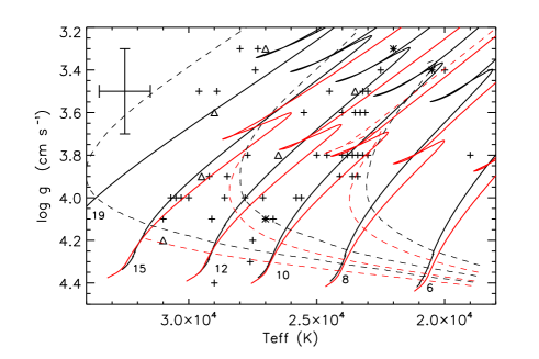
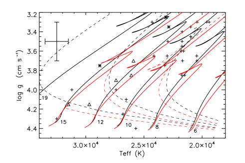
Figure 3: Estimates of the atmospheric parameters for the targets from the VFTS (upper) and FLAMES-I survey (lower); some targets have been moved slightly in effective temperature to improve clarity. Targets with an estimated nitrogen abundance, 7.2$\leq$$\epsilon_{\rm{N}}$$<$7.5 dex, are shown as asterisks and those with $\epsilon_{\rm{N}}$$\geq$7.5 dex are shown as triangles; all other targets are shown as crosses. Evolutionary models of Brott et al. (2011a) (solid black lines) and Georgy et al. (2013b) (solid red lines) are shown for zero initial rotational velocity together with the initial mass (in units of the solar mass). Isochrones (dashed lines) are shown as dotted lines with the same colour selection for ages of 5, 10 and 20 Myr. Typical uncertainties in the effective temperatures and gravity estimates are also shown.

The estimated projected rotational velocities of our two samples lie between 0–80 km s^-1 due to the selection criteria and in the subsequent discussion two ranges are considered, viz, $v_{\rm{e}}\sin i$ $\leq$40 km s^-1 and 40 $<$ $v_{\rm{e}}\sin i$ $\leq$ 80 km s^-1. The VFTS estimates of Dufton et al. (2013) adopted a Fourier Transform methodology (see, Carroll 1933; Simón-Díaz & Herrero 2007, for details), whilst the FLAMES-I measurements of Hunter et al. (2008b) were based on profile fitting of rotationally broadened theoretical spectra to the observations.

As discussed by Simón-Díaz & Herrero (2014), both methods can be subject to errors due the effects of other broadening mechanisms, including macroturbulence and microturbulence. They concluded that for O-type dwarfs and B-type supergiants, estimates for targets with $v_{\rm{e}}\sin i$ $\leq$ 120 km s^-1 could be overestimated by $\sim$25$\pm 20$ km s^-1. Recently Simón-Díaz et al. (2017b) have discussed in detail the non-rotational broadening component in OB-type stars. They again find that their O-type stellar and B-type supergiant samples are ’dominated by stars with a remarkable non-rotational broadening component’; by contrast, in the B-type main sequence domain, the macroturbulence estimates are generally smaller, although the magnitude of any uncertainty in the projected rotational velocity is not quantified. However inspection of Fig.5 of Simón-Díaz et al. (2017b), implies that the macroturbulence will be typically 20-30 km s^-1 in our targets compared with values of 100 km s^-1 or more that can be found in O-type dwarfs and OB-type supergiants.

The effects of these uncertainties on our samples are expected to be limited for three reasons. Firstly the results of Simón-Díaz et al. (2017b) imply that the effects of non-rotational broadening components are likely to be smaller in our sample than in the O-type stellar and B-type supergiants discussed by Simón-Díaz & Herrero (2014). Secondly, we have not used specific $v_{\rm{e}}\sin i$ estimates but rather placed targets into $v_{\rm{e}}\sin i$  bins. Thirdly for our sample and especially the cohort with $v_{\rm{e}}\sin i$ $\leq$ 40 km s^-1, the intrinsic narrowness of the metal line spectra requires a small degree of rotational broadening. In Sect. 6.4, we discuss the implications of possible uncertainties in our $v_{\rm{e}}\sin i$  estimates.

6.2 Nitrogen abundances

As discussed by Garland et al. (2017), the LMC baseline nitrogen abundance has been estimated from both H ii regions and early-type stars. For the former, Kurt & Dufour (1998) and Garnett (1999) found 6.92 and 6.90 dex respectively. Korn et al. (2002, 2005), Hunter et al. (2007) and Trundle et al. (2007b) found a range of nitrogen abundances from their analyses of B-type stellar spectra, which they attributed to different degrees of enrichment by rotational mixing. Their lowest estimates implied baseline nitrogen abundances of 6.95 dex (1 star), 6.90 dex (5 stars) and 6.88 dex (4 stars) respectively. These different studies are in good agreement and a value of 6.9 dex has been adopted here, which is -0.93 dex lower than the solar estimate (Asplund et al. 2009)

The majority of targets appear to have nitrogen abundances close to this baseline, with approximately 60% of the 54 VFTS targets and 75% of the 34 FLAMES-I targets having enhancements of less than 0.3 dex. Additionally for the VFTS sample, an additional 20% of the sample have upper limits greater than 7.2 dex but could again either have modest or no nitrogen enhancements. Hence approximately three quarters of each sample may have nitrogen enhancements of less than a factor of two. This would, in turn be consistent with them having relatively small rotational velocities and having evolved without any significant rotational mixing (see, for example, Maeder 1987; Heger & Langer 2000; Maeder 2009; Frischknecht et al. 2010).

The two targets, VFTS 167 and 469 whose spectroscopy was probably affected by fibre cross-contaminations (see Sect. 2), have atmospheric parameters that are consistent with both their spectral types and other VFTS targets. Additionally they appear to have near baseline nitrogen abundances. Although these results should be treated with some caution, it appears unlikely that they belong to the subset of targets with large nitrogen enhancements discussed below.

Two targets, VFTS 237 and 835, have been identified as Be-type stars and might be expected to show the effects of rotational mixing due to rotational velocities near to critical velocities having been inferred (Townsend et al. 2004; Cranmer 2005; Ahmed & Sigut 2017) for such objects. However both have near baseline nitrogen abundance estimates (6.92 and 6.90 dex respectively) implying that little rotational mixing has occurred. Our analysis did not make any allowance for the effects of light from a circumstellar disc. Dunstall et al. (2011) analysed spectroscopy of 30 Be-type stars in the Magellanic Clouds and estimated a wide range of disc contributions, $\sim$0-50%. In turn this led to increases in their nitrogen abundances in the range $\sim$0-0.6 dex with a median increase of 0.2 dex. Hence a nitrogen enhancement in these two objects cannot be discounted. However near baseline nitrogen abundances have previously been found for Be-type stars in both the Galaxy (Ahmed & Sigut 2017) and the Magellanic Clouds (Lennon et al. 2005; Dunstall et al. 2011), with Ahmed & Sigut (2017) having recently discussed possible explanations.

The remaining targets show significant enhancements in nitrogen of up to 1.0 dex. For both samples, $\sim$20-25% show an enhancement of greater than 0.3 dex with $\sim$10-15% having enhancements of greater than 0.6 dex. These could be rapidly rotating stars that have undergone rotational mixing and are being observed at small angles of inclination. However such cases would be expected to be relatively rare. For example, assuming random axes of inclination, a star with an equatorial velocity of 300 km s^-1 would have a value of $v_{\rm{e}}\sin i$ $\leq$40 km s^-1 only about 1% of the time. Additionally the probability that such a star would be observed with 40 $<$ $v_{\rm{e}}\sin i$ $\leq$ 80 km s^-1 is approximately four times that of it being observed with $v_{\rm{e}}\sin i$ $\leq$ 40 km s^-1. Similar ratios would be found for other values of the rotational velocity and just reflects the greater solid angle of inclination available to stars in the larger projected rotational velocity bin. By contrast, the nitrogen rich targets in our samples are more likely to have $v_{\rm{e}}\sin i$ $\leq$ 40 km s^-1 than 40 $<$ $v_{\rm{e}}\sin i$ $\leq$ 80 km s^-1, as can be seen from Table 7. In Sect. 6.3, we return to these objects and undertake simulations to investigate whether all the nitrogen enhanced stars in our sample could indeed be fast rotators observed at small angles of inclination.

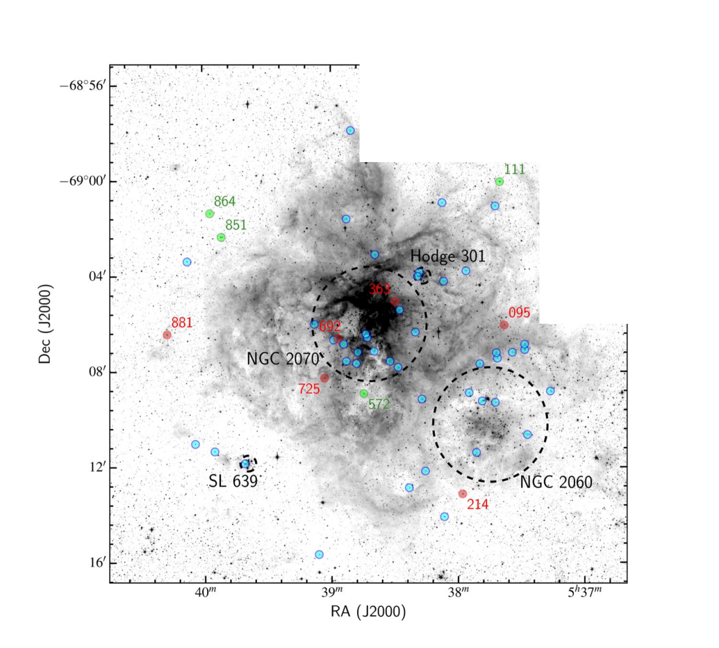
Figure 4: Spatial distribution of the VFTS targets in 30 Doradus. Targets with 7.2$\leq$$\epsilon_{\rm{N}}$$<$7.5 dex, are shown in green and those with $\epsilon_{\rm{N}}$$\geq$7.5 dex in red; other targets are shown in blue. The spatial extents of NGC 2070, NGC 2060, SL 639, and Hodge 301 (Evans et al. 2015) are indicated by the overlaid dashed circles. The underlying image is from a V-band mosaic taken with the ESO Wide Field Imager on the 2.2 m telescope at La Silla.

We have investigated the other observed characteristics of our nitrogen enhanced stars to assess whether they differ from those of the rest of the sample. Fig. 4 shows the spatial distribution of all of our VFTS targets, together with the position and extent of the larger clusters NGC 2070 and NGC 2060 and the smaller clusters, Hodge 301 and SL639; the sizes of the clusters should be treated as representative and follow the definitions of Evans et al. (2015, Table 4). The nitrogen enriched targets are distributed across the 30 Doradus region with no evidence for clustering within any cluster. Adopting the cluster extents of Evans et al. (2015), there are 21 cluster and 33 field VFTS stars. All four targets with 7.2$\leq$$\epsilon_{\rm{N}}$$<$7.5 dex lie in the field whilst those with $\epsilon_{\rm{N}}$$\geq$7.5 dex consist of four field and two cluster stars. Hence of the ten nitrogen enriched stars, only two lie in a cluster implying a possible excess of field stars. However simple binomial statistics, imply that this excess is not significant at the 10% level for either the total sample or those in the two abundance ranges.

The dynamics of our sample can also be investigated using the radial velocity measurements summarised in Table 1. The mean radial velocity for the whole sample is 270.3$\pm$16.6 km s^-1 (54 targets), whilst the 10 nitrogen enriched stars and the remaining 44 stars have values of $270.2\pm 18.9$km s^-1 and $270.3\pm 16.3$km s^-1 respectively. The latter two means are very similar whilst an F-test of the corresponding variances showed that they were not significantly different at even the 20% level. Hence we conclude that the radial velocity distributions of the two subgroups appear similar within the limitation of the sample sizes.

A comparison of the atmospheric parameters also reveals no significant differences. For example, the whole VFTS sample have a median and mean effective temperature of 27 000 and 25 865 K, while the values for the targets with $\epsilon_{\rm{N}}$$\geq$7.2 dex are 26 500 and 26056 K. The corresponding statistics for the gravity are 3.80/3.77 dex (whole sample) and 3.75/3.74 dex (nitrogen enriched) and for the microturbulence 1.5/2.6 km s^-1 (whole sample) and 2.0/2.2 km s^-1 (nitrogen enriched).

A helium to hydrogen abundance ratio by number of 0.1 was assumed in our calculations of theoretical spectra (see Sect. 4.1). The LMC evolutionary models of Brott et al. (2011a) appropriate to B-type stars indicate that even for a nitrogen enhancement of 1.0 dex (which is the largest enhancement observed in our sample – see Tables 3 and 5), the change in the helium abundance is typically only 0.03 dex. Hence our assumption of a normal helium abundance is unlikely to be a significant source of error. We have checked this by comparing theoretical and observed He i profiles for targets with the largest nitrogen enhancements. This comparison was impacted by significant nebula emission especially for lines in the (3d)³D-(4f)³F series but generally yielded good agreement between observation and theory for our adopted helium abundance.

This is illustrated by observed and theoretical spectra of the wavelength region 3980-4035 Å shown in Fig. 5 for VFTS 650 and 725, which have similar atmospheric parameters. The observed spectra have been corrected using the radial velocity estimates listed in Table 1, while the theoretical spectra have been interpolated from our grid to be consistent with the atmospheric parameters and nitrogen abundances listed in Table 3. The latter have also been convolved with a Gaussian function to allow for instrumental broadening; as both stars have estimated projected rotational velocities, $\leq$ 40 km s^-1, no correction was made for rotational broadening. For the two diffuse He i lines at approximately 4009 and 4026 Å, the agreement is excellent although VFTS 650 has a near baseline nitrogen abundance whilst VFTS 725 has the second highest nitrogen abundance in the VFTS sample. The agreement between theory and observation for the N ii at 3995 Å is also good and supports our use of equivalent widths to estimate element abundances. The observed spectra also illustrate the range of observed S/N with VFTS 650 (S/N$\sim$60) and 725 (S/N$\sim$120) having estimates towards to the lower and upper ends of that observed.

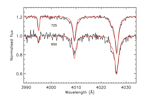
Figure 5: Observed and theoretical spectra for the wavelength region near 4000 Å in two stars, VFTS 650 and 725. Atmospheric parameters and nitrogen abundances were taken from Table 3 for the theoretical spectra. The normalised spectra for VFTS 725 have been shifted upwards to improve clarity

For the nitrogen enriched stars, changes in the carbon and oxygen abundances would also be expected. Maeder et al. (2014) argued that comparison of the relative N/C and N/O abundances would provide a powerful diagnostic of rotational mixing. The LMC models of Brott et al. (2011a) appropriate to B-type stars indicate that for a nitrogen enhancement of $\sim$1.0 dex, the carbon and oxygen abundances would be decreased by -0.22–0.35 dex and -0.08–0.10 dex respectively.

Unfortunately the strongest C ii line in the blue spectra of B-type stars is the doublet at 4267 Å, which is badly affected by nebular emission. Due to the sky and stellar fibres being spatially separated, it was not possible to reliably remove this emission from the VFTS spectroscopy. Indeed as discussed by McEvoy et al. (2015) this can lead to the reduced spectra having spurious narrow emission or absorption features. This is especially serious for targets with small projected rotational velocities, where the width of the nebular emission is comparable with that of the stellar absorption lines. No other C ii lines were reliably observed in the VFTS spectra and hence reliable carbon abundances could not be deduced. The FLAMES-I spectroscopy may also be affected by nebular emission although this might be expected to be smaller especially in the older cluster, NGC2004. However without a reliable method to remove nebular emission, the approach advocated by Maeder et al. (2014) would appear to be of limited utility for multi-object fibre spectroscopy of low $v_{\rm{e}}\sin i$ early-type stars.

Both the VFTS and FLAMES-I data have rich O ii spectra. However the predicted changes in the oxygen abundance (of less than 0.1 dex) are too small to provide a useful constraint, given the quality of the observational data. This is confirmed by the original FLAMES-I analyses (Hunter et al. 2007, 2008a, 2009; Trundle et al. 2007b), where for the targets considered here an oxygen abundance of 8.38$\pm$0.15 dex was found (which is lower than the solar estimate by -0.31 dex, Asplund et al. 2009). The standard error is similar to that found in Sect. 4.5 for the magnesium abundance where no variations within our sample are expected. Additionally for the five FLAMES-I stars with a nitrogen enhancement of more than 0.6 dex, the mean oxygen abundance was 8.40$\pm$0.08 consistent with that found for all the targets.

Table 6: Estimates of the initial rotational velocity, $v_{\rm{i}}$, required to achieve nitrogen enhancements of greater than 0.3 dex ($\epsilon_{\rm{N}}$$\geq$7.2 dex) and 0.6 dex ($\epsilon_{\rm{N}}$$\geq$7.5 dex) whilst maintaining a gravity, $\log g$ $\geq$ 3.3 dex. Also listed are the minimum rotational velocities, $v_{\rm{e}}$, predicted by the models during this evolutionary phase. Initial masses ( $\rm{M}_{\rm{i}}$) are in units of the solar mass,  $\rm{M}_{\odot}$. The values characterised as ’Adopted’ were used in the simulations discussed in Sects. 6.3-6.5.

$\rm{M}_{\rm{i}}$/ $\rm{M}_{\odot}$	$\epsilon_{\rm{N}}$$\geq$7.2 dex		$\epsilon_{\rm{N}}$$\geq$7.5 dex
	$v_{\rm{i}}$	$v_{\rm{e}}$	$v_{\rm{i}}$	$v_{\rm{e}}$
	km s-1	km s-1	km s-1	km s-1
5	180	142	258	219
8	161	132	230	207
12	163	140	219	200
16	144	130	217	203
Adopted	145	135	220	205

Table 7: Observed and predicted numbers of nitrogen rich targets with enhancements of greater than 0.3 dex ($\epsilon_{\rm{N}}$$\geq$7.2 dex) and 0.6 dex ($\epsilon_{\rm{N}}$$\geq$7.5 dex). The Monte-Carlo simulations are designated as ’MC’. When two number of targets, $N$, are listed, they refer to simulations tailored to the different nitrogen abundance limits as discussed in the text. The rotational velocity distribution, $f(v_{\mathrm{e}})$, is either from Dufton et al. (2013, VFTS) or from the deconvolution illustrated in Fig. 6 (FLAMES-I). Simulations are provided for two ranges of projected rotational velocity, $v_{\rm{e}}\sin i$, viz. 0-40 km s^-1 and 40-80 km s^-1.

Sample	$N$	$f(v_{e})$	$\epsilon_{\rm{N}}$$\geq$7.2		$\epsilon_{\rm{N}}$$\geq$7.5
$v_{\rm{e}}\sin i$ (km s-1)			0-40	40-80	0-40	40-80
VFTS sample
Observed	255	-	7	3	5	1
MC	255	VFTS	2.30$\pm$1.50	7.17$\pm$2.63	1.45$\pm$1.18	4.46$\pm$2.08
MC Prob (%)	255	VFTS	0.8	7	2	6
MC	220/188	VFTS	1.98$\pm$1.14	5.29$\pm$2.27	1.25$\pm$1.11	3.32$\pm$1.80
MC Prob (%)	220/188	VFTS	0.4	22	0.9	16
FLAMES-I sample
Observed	103	-	6	2	4	1
MC	103	VFTS	0.92$\pm$0.96	2.89$\pm$1.69	0.58$\pm$0.76	1.82$\pm$1.33
MC Prob(%)	103	VFTS	0.03	45	0.3	46
MC	73	FLAMES-I	0.57$\pm$0.76	1.82$\pm$1.33	0.26$\pm$0.51	0.79$\pm$0.89
MC Prob(%)	73	FLAMES-I	0.01	55	0.04	56

6.3 Estimation of numbers of nitrogen enriched targets

As discussed above, it is unclear whether the targets with the largest nitrogen enhancements in our samples could have evolved as single stars undergoing rotational mixing. We have therefore undertaken simulations to estimate the number of rotationally mixed stars that we might expect to find in our sample. We have considered two thresholds for nitrogen enrichment, viz. 0.3 dex (corresponding to a nitrogen abundance, $\epsilon_{\rm{N}}$$>$7.2 dex) and 0.6 dex ($\epsilon_{\rm{N}}$$>$7.5 dex). The former was chosen so that any enhancement would be larger than the estimated errors in the nitrogen abundances, whilst the larger was chosen in an attempt to isolate the highly enriched targets, at least in terms of those lying near to the main sequence. As discussed by McEvoy et al. (2015), B-type supergiants (both apparently single stars and those in binary systems) in 30 Doradus can exhibit larger nitrogen abundances, $\epsilon_{\rm{N}}$, of up to 8.3 dex corresponding to an enhancement of 1.4 dex; however these stars have probably evolved from the O-type main sequence. The number of stars fulfilling these criteria in both the VFTS and FLAMES-I samples are summarised in Table 7.

We have used the LMC grid of models of Brott et al. (2011a) to estimate the initial stellar rotational velocities, $v_{\rm{i}}$, that would be required to obtain such enrichments. The core hydrogen burning phase, where the surface gravity, $\log g$ $\geq$ 3.3 dex, was considered in order to be consistent with the gravities estimated for our samples (see Tables 3 and 5). We have also found the minimum rotational velocity, $v_{\rm{e}}$, that a star would have during this evolutionary phase; this velocity was normally found at a gravity, $\log g$ $\simeq$3.3 dex. The initial masses were limited to 5-16 $\rm{M}_{\odot}$ as the ZAMS effective temperatures in this evolutionary phase range from approximately 20 000 to 33 000K, compatible with our estimated effective temperatures, again listed in Tables 3 and 5.

For each initial mass, we have quadratically interpolated between models with different initial ($v_{\rm{i}}$) rotational velocities to estimate both the initial ($v_{\rm{i}}$) and the minimum rotational velocity ($v_{\rm{e}}$ - hereafter designated as ‘the current rotational velocity’) that would achieve a nitrogen enhancement of at least either 0.3 or 0.6 dex whilst the surface gravity, $\log g$ $\geq$ 3.3 dex. These estimates are summarised in Table 6. Given that the grid spacing in the initial rotational velocity was typically 60 km s^-1 (or less), we would expect that the interpolation would introduce errors of less than 20 km s^-1. The ranges of the estimated initial and current velocities for different masses are approximately 20% and 15% respectively. For our simulations, we have taken a conservative approach and adopted velocities (see Table 6) at the lower ends of our estimates. In turn this will probably lead to an overestimate in the number of targets with enhanced nitrogen abundances and small projected rotational velocities in our simulations. This overestimation will be re-enforced by the adoption of a lower gravity limit, $\log g$ $\geq$3.3 dex whilst our estimated gravities are generally larger; for example over half the VFTS sample have estimated gravities, $\log g$ $\geq 3.8$ dex.

As discussed by Gray (2005), for a random distribution of rotation axes, the probability distribution for observing an angle of inclination, $i$, is:

$$P(i)\ di=\sin i\ di$$ (1)

the probability of observing an angle of inclination, $i\leq i_{0}$ is then given by:

$$P(i\leq i_{0})=1-\cos i_{0}$$ (2)

For a sample of $N$ targets with a normalised rotational velocity distribution, $f(v_{e})$, the number that will have a projected rotational velocity less than $v^{\prime}$ is given by:

$$N(v_{e}\sin i\leq v^{\prime})=N\left[\int^{v^{\prime}}_{0}f(v_{e})dv_{e}+\int^{\infty}_{v^{\prime}}f(v_{e})P\left(i\leq i_{0}\right)dv_{e}\right]$$ (3)

or

$$N(v_{e}\sin i\leq v^{\prime})=N\left[\int^{v^{\prime}}_{0}f(v_{e})dv_{e}+\int^{\infty}_{v^{\prime}}f(v_{e})\left(1-\cos i_{0}\right)dv_{e}\right]$$ (4)

where

$$i_{0}=\sin^{-1}\left(\frac{v^{\prime}}{v_{e}}\right)$$ (5)

The number of targets that have both $v_{\rm{e}}\sin i$ $\leq v^{\prime}$ and a nitrogen enhancement, $\epsilon_{\rm{N}}$$\geq$$\epsilon_{\rm{0}}$, can then be estimated by changing the lower limits of integration in equation 4 to the rotational velocities, $v_{\rm{e}}$, summarised in Table 6. This will normally eliminate the first term on the right hand side of equation 4 leading to:

$$\begin{split}N(v_{e}\sin i\leq v^{\prime};\epsilon\geq\epsilon_{\mathrm{0}})=N\int^{\infty}_{v_{\mathrm{e}}}f(v_{e})\left[1-\cos i_{0}\right]dv_{e}\end{split}$$ (6)

The rotational velocity distribution, $f(v_{e})$, for the VFTS B-type single star sample has been deduced by Dufton et al. (2013, see their Table 6). Hunter et al. (2008b) assumed a single Gaussian distribution for the rotational velocities in the FLAMES-I single B-type star sample and fitted this to the observed $v_{\rm{e}}\sin i$ distribution. We have taken their observed values and used the deconvolution methodology of Lucy (1974) as described in Dufton et al. (2013) to estimate $f(v_{e})$ for the FLAMES-I sample. This is shown in Fig. 6 together with that for the VFTS sample (Dufton et al. 2013). They both show a double peaked structure although there are differences in the actual distributions. The number of $v_{\rm{e}}\sin i$ estimates in the FLAMES-I sample was relatively small (73) and may have some additional selection effects compared with the VFTS sample as discussed in Sect. 6.4. We have therefore adopted the $f(v_{e})$ from the VFTS B-type single star sample in most of our simulations but discuss this choice further below.

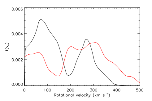
Figure 6: The de-convolved rotational velocity distribution, $f(v_{e})$, for the LMC FLAMES-I sample of single B-type targets with luminosity classes V to III (black line) compared with that for the equivalent VFTS sample taken from Dufton et al. (2013, red line).

Evans et al. (2015) classified 434 VFTS targets as B-type and subsequently Dunstall et al. (2015) found 141 targets (including 40 supergiants) to be radial velocity variables. McEvoy et al. (2015) identified an additional 33 targets as single B-type supergiants, leading to 260 remaining targets. However the relatively low data quality of five of these targets prevented Dufton et al. (2013) estimating projected rotational velocities. Hence we have adopted $N=255$ for the number of B-type VFTS targets which have luminosity classes V to III and have estimated projected rotational velocities. For the FLAMES-I sample, Evans et al. (2006) has provided spectral types including targets classified as Be-Fe without a luminosity classification. As they are likely to be lower luminosity objects, they were included when deducing a value of $N=103$. Using these sample sizes, we have numerically integrated Equation 6 in order to predict the number of nitrogen enriched targets. To validate these results and also to estimate their uncertainties, we have also undertaken a Monte-Carlo simulation. Samples of $N$ targets were randomly assigned both rotational velocities (using the rotational velocity distribution, $f(v_{e})$ discussed above) and angles of inclination (using equation 1). The number of targets with different nitrogen enrichments and in different projected rotational bins were then found using the rotational velocity limits in Table 6.

Our simulations are all based on the assumption that the rotational axes of our targets are randomly orientated. As can be seen from Fig. 4, approximately half our targets are situated in four different clusters (with different ages, see, for example, Walborn & Blades 1997; Evans et al. 2011, 2015) with the remainder spread across the field. Such a diversity of locations would argue against them having any axial alignment. However Corsaro et al. (2017) identified such alignments in two old Galactic open clusters, although previously Jackson & Jeffries (2010) found no such evidence in two younger Galactic clusters. If the VFTS axes were aligned, the identification by Dufton et al. (2013) of B-type stars with projected rotational velocities, $v_{\rm{e}}\sin i$ $>$ 400 km s^-1 (which is close to their estimated critical velocities Huang et al. 2010; Townsend et al. 2004), would then imply a value for the inclination axis, $\sin i$ $\simeq$ 1. In turn this would lead to all our targets having small rotational velocities thereby exacerbating the inconsistencies illustrated in Table 7.

6.4 Comparison of simulations with numbers of observed nitrogen enriched targets

The numerical integrations and the Monte Carlo simulations led to results that are indistinguishable, providing reassurance that the methodologies were correctly implemented. The Monte-Carlo simulations are summarised in Table 7, their standard errors being consistent with Poisson statistics which would be expected given the low probability of observing stars at low angles of inclination. For both samples, the simulations appear to significantly underestimate the number of nitrogen enriched targets with $v_{\rm{e}}\sin i$ $\leq$ 40 km s^-1 and possibly overestimate those with 40 $<$ $v_{\rm{e}}\sin i$$\,\leq$ 80 km s^-1.

We have therefore used the Monte-Carlo simulations to find the probabilities of observing the number of nitrogen enriched stars summarised in Table 7. When the observed number, $n$ was greater than predicted, we calculated the probability that the number observed would be greater than or equal to $n$. Conversely, when the observed number, $n$ was less than predicted, we calculated the probability that the number observed would be less than or equal to $n$. These probabilities are also listed in Table 7 and again very similar probabilities would have been found from adopting Poisson statistics. All the differences for the targets with $v_{\rm{e}}\sin i$ $\leq$ 40 km s^-1 are significant at the 5% level. By contrast for the samples with 40 $<$ $v_{\rm{e}}\sin i$$\,\leq$ 80 km s^-1, none are significant at the 5% level.

For the VFTS Monte-Carlo simulations, the choice of $N=255$ leads to 36$\pm$6 and 31$\pm$5 targets with $v_{\rm{e}}\sin i$ $\leq$ 40 km s^-1 and 40 $<$ $v_{\rm{e}}\sin i$$\,\leq$ 80 km s^-1 respectively. As expected these are in good agreement with the 37 and 30 targets in the original sample in Table 1. However thirteen of these targets were not analysed, reducing the sample summarised in Table 3 to 31 ($v_{\rm{e}}\sin i$ $\leq$ 40 km s^-1) and 23 (40 $<$ $v_{\rm{e}}\sin i$$\,\leq$ 80 km s^-1) targets. We have therefore repeated the Monte Carlo simulations using values of $N$  (220 and 188 respectively) that reproduce the number of targets actually analysed. These simulations are also summarised in Table 7 and again lead to an overabundance of observed nitrogen enriched targets with $v_{\rm{e}}\sin i$ $\leq$ 40 km s^-1 that is now significant at 1% level. By contrast the simulations are consistent with the observations for the cohort with 40 $<$ $v_{\rm{e}}\sin i$$\,\leq$ 80 km s^-1.

Even after allowing for the targets that were not analysed, the discrepancy between the observed number of VFTS targets with $v_{\rm{e}}\sin i$ $\leq$ 40 km s^-1 and the simulations may be larger than predicted. As discussed above, both the conservative current rotational velocities, $v_{\rm{e}}$, adopted in Table 6 and the decision to follow the stellar evolution to a logarithmic gravity of 3.3 dex will lead to the simulations being effectively upper limits. Additionally, for the VFTS subsample with $v_{\rm{e}}\sin i$ $\leq$ 40 km s^-1, there are seven targets, where the upper limit on the nitrogen abundance was consistent with $\epsilon_{\rm{N}}$$>$7.2 dex and four targets consistent with $\epsilon_{\rm{N}}$$>$7.5 dex. If any of these had significant nitrogen enhancements that would further increase the discrepancies for this cohort.

The simulations for the smaller FLAMES-I sample are consistent with those for the VFTS sample. For a sample size of $N=103$, the number of nitrogen enriched stars with $v_{\rm{e}}\sin i$ $\leq$ 40 km s^-1  is greater than predicted for both $\epsilon_{\rm{N}}$$\geq$7.2 dex and $\epsilon_{\rm{N}}$$\geq$7.5 dex. Indeed the Monte-Carlo simulation implies that this difference is significant at the 1% level. By contrast the cohort with 40 $<$ $v_{\rm{e}}\sin i$$\,\leq$ 80 km s^-1 is compatible with the simulations. The re-evaluation of the nitrogen abundance estimates in Sect. 4.6 led to a decrease in the number of targets with $\epsilon_{\rm{N}}$$>$7.2 dex by four. All these targets (NGC2004/43, 84, 86 and 91) had $v_{\rm{e}}\sin i$ $\leq$ 40 km s^-1 and adopting the previous nitrogen abundance estimates would have further increased the discrepancy with the simulations for this cohort. The re-evaluation also moved one target into the $\epsilon_{\rm{N}}$$>$7.5 dex cohort. However this target (NGC2004/70) has an estimated $v_{\rm{e}}\sin i$= 46 km s^-1  and hence this change would not affect the low probabilities found for the nitrogen enhanced targets with $v_{\rm{e}}\sin i$ $\leq$ 40 km s^-1.

The FLAMES-I results should however be treated with some caution. Firstly, although there were multi-epoch observations for the this sample, the detection of radial-velocity variables (binaries) was less rigorous than in the VFTS observations; this is discussed further in Sect. 6.6.4. Secondly, the exclusion of a number of Be-type stars in the original target selection for NGC 2004 may have led to this sample being biased to stars with lower values of the rotational velocity (see Brott et al. 2011b, for a detailed discussion of the biases in this sample). Hence, the use of the VFTS rotational-velocity distribution, $f(v_{e})$, may not be appropriate for the FLAMES-I sample. There is some evidence for this in that the observed number of FLAMES-I targets (18 with $v_{\rm{e}}\sin i$ $\leq$ 40 km s^-1 and 16 with 40 $<$ $v_{\rm{e}}\sin i$$\,\leq$ 80 km s^-1) is larger than that predicted (14.5$\pm$3.5 and 12.6$\pm$3.3 respectively). This would be consistent with the $f(v_{e})$ distribution for the FLAMES-I sample shown in Fig. 6 being weighted more to smaller rotational velocities than the VFTS distribution that was adopted. We have therefore also used the $f(v_{e})$ distribution, together with the number of $v_{\rm{e}}\sin i$ estimates, $N=73$ deduced for the FLAMES-I sample in the Monte Carlo simulation and the results are again summarised in Table 7. This leads to even lower probabilities for the observed number of nitrogen enhanced targets with $v_{\rm{e}}\sin i$ $\leq$ 40 km s^-1 being consistent with the simulations, whilst the probabilities for the 40 $<$ $v_{\rm{e}}\sin i$$\,\leq$ 80 km s^-1 cohort are increased. The predicted number of targets in the two $v_{\rm{e}}\sin i$ ranges (15.5$\pm$3.5 and 16.6$\pm$3.6 respectively) are now in better agreement with those observed.

As discussed in Sect. 6.1, our adopted $v_{\rm{e}}\sin i$ estimates may be too high. Simón-Díaz & Herrero (2014) estimated that this might be typically 25$\pm$20 km s^-1 for O-type stars and B-type supergiants; the effects on our samples of B-type dwarfs and giants are likely to be smaller given their smaller macroturbulences (Simón-Díaz et al. 2017b). However we have considered the effect of arbitrarily decreasing all our $v_{\rm{e}}\sin i$ estimates by 20 km s^-1. This would move eleven VFTS targets and seven FLAMES-I targets into the $v_{\rm{e}}\sin i$ $\leq$ 40 km s^-1 bins. Similar numbers of targets would also be moved into the 40 $<$ $v_{\rm{e}}\sin i$$\,\leq$ 80 km s^-1 bins from higher projected rotational velocities but as these targets have not been analysed, we are unable to quantitatively investigate the consequences for this bin. However we note that the simulation showed that the predicted number of targets in the 40 $<$ $v_{\rm{e}}\sin i$$\,\leq$ 80 km s^-1 bin were consistent with that observed and it is likely that this result would remain unchanged.

For the cohorts with $v_{\rm{e}}\sin i$$\leq$ 40 km s^-1, the numbers would be increased to 48 (VFTS) and 24 (FLAMES-I). However the number of targets with $\epsilon_{\rm{N}}$$>$7.2 or 7.5 dex would also be increased to eight and six (VFTS) and eight and five (FLAMES-I) respectively. We have undertaken Monte-Carlo simulations that reproduce the total number of targets with $v_{\rm{e}}\sin i$ $\leq$ 40 km s^-1 by increasing the B-type samples to $N$=$335$ (VFTS) and 170 (FLAMES-I). These simulations again lead to small probabilities of observing the relatively large numbers of nitrogen enhanced targets, viz $<2$% (VFTS) and $<0.1$% (FLAMES-I). This arbitrary decrease in the $v_{\rm{e}}\sin i$ estimates would also affect the rotational velocity function, $f(v_{e})$, used in the simulations. If applied universally, this would shift the distribution to smaller rotational velocities, thereby decreasing the predicted number of nitrogen enhanced targets. Additionally either allowing for VFTS targets without nitrogen abundance estimates or the use of the FLAMES-I rotational velocity distribution shown in Fig. 6 would also decrease the predicted numbers and hence probabilities.

Inspection of the metal absorption lines in the spectra for the targets moved into the $v_{\rm{e}}\sin i$ $\leq$ 40 km s^-1 bin showed that they generally had the bell shaped profile characteristic of rotational broadening. Hence we believe that the arbitrary decrease of 20 km s^-1 probably overestimates the magnitude of any systematic errors. As such, we conclude that uncertainties in the $v_{\rm{e}}\sin i$ estimates are very unlikely to provide an explanation for the discrepancy between the observed and predicted numbers of nitrogen enriched targets in the cohort with $v_{\rm{e}}\sin i$ $\leq$ 40 km s^-1.

In summary, the simulations presented in Table 7 are consistent with the nitrogen enriched targets for both the VFTS and FLAMES-I samples with 40 $<$ $v_{\rm{e}}\sin i$$\,\leq$ 80 km s^-1 having large rotational velocities (and small angle of incidence) leading to significant rotational mixing. By contrast, there would appear to be too many nitrogen enriched targets in both samples with $v_{\rm{e}}\sin i$ $\leq$ 40 km s^-1 to be accounted for by this mechanism.

6.5 Frequency of nitrogen enriched, slowly rotating B-type stars

The simulations presented in Sect. 6.4 imply that there is an excess of targets with $v_{\rm{e}}\sin i$ $\leq$ 40 km s^-1 and enhanced nitrogen abundances. In the VFTS sample, there are two objects with a nitrogen abundance, 7.2$\leq$$\epsilon_{\rm{N}}$$<$7.5 dex. Our Monte-Carlo simulations imply that there should be 0.85$\pm$0.92 and that the probability of observing two or more objects would be approximately 20%. Hence their nitrogen enhancement could be due to rotational mixing, although we cannot exclude the possibility that they are indeed slowly rotating. In turn this implies that the excess of targets with high nitrogen abundances appears to occur principally for $\epsilon_{\rm{N}}$$\geq$7.5 dex. Additionally the small number of such objects in the cohort with 40 $<$ $v_{\rm{e}}\sin i$$\,\leq$ 80 km s^-1 further implies that these objects have rotational velocities, $v_{e}\leq 40$km s^-1.

In the subsequent discussion, we will consider two percentages, viz. firstly the percentage, P₄₀, of stars within the cohort with $v_{e}\leq$40 km s^-1 that have enhanced nitrogen abundances that do not appear to be due to rotational mixing and secondly the percentage, P_T, of such stars within the total population of single stars with luminosity classes III-V. Our simulations indicate that 67% of the 31 VFTS targets with $v_{\rm{e}}\sin i$ $\leq$ 40 km s^-1 will also have $v_{e}\leq$40 km s^-1, equating to $\sim$21 targets. From the simulations summarised in Table 7, the excess of VFTS objects with $\epsilon_{\rm{N}}$$\geq$7.5 dex and $v_{\rm{e}}\sin i$ $\leq$ 40 km s^-1  is 3.55-3.75 depending on the value of $N$ adopted. This would then imply a percentage of such objects, P₄₀$\sim$18%. This may be an underestimate as there are four targets with $v_{e}\leq 40$km s^-1, whose nitrogen abundance cannot be constrained to less than 7.5 dex and excluding these would increase the percentage to P₄₀$\sim$21%. A similar calculation for the FLAMES-I sample leads to a higher fraction of P₄₀$\sim$30–33% depending on the simulation adopted, with no correction now being required for stars whose nitrogen abundance could not be constrained.

These percentages then translate in to percentages with respect to the whole population B-type stars of P_T$\sim$1.5–2.0% and 3.4–3.7% for the VFTS and FLAMES-I samples respectively. The latter is significantly smaller than the fraction of slow rotators found by Hunter et al. (2008a) that showed significant nitrogen enrichment, which was estimated as approximately 20% of the non-binary core hydrogen burning sample. However the two estimates are not directly comparable for the following reasons.

Firstly Hunter et al. (2008a) adopted a larger projected rotational velocity range, $v_{\rm{e}}\sin i$ $\leq$ 50 km s^-1, to that adopted here. Secondly they defined a significant nitrogen enrichment as $\epsilon_{\rm{N}}$$\geq$7.2 dex rather than the larger value adopted here. Thirdly they selected all targets with estimated effective temperatures $T_{\mathrm{eff}}$ $\leq$ 35 000 K and gravities $\log g$ $\geq$ 3.2 dex. These included some late O-type stars, supergiants and binaries. Fourthly they made no allowance for the targets with  $\leq$ 50 km s^-1 but with a rotational velocity sufficient to produce the observed nitrogen abundance by rotational mixing. Finally they adopted for their LMC non-binary core hydrogen burning sample the 73 apparently single targets that had estimates for their projected rotational velocity. However as discussed in Sect. 6.4, Evans et al. (2005) lists 103 B-type non-supergiant stars with no evidence for binarity and we have adopted this larger sample size in our simulations.

Hunter et al. (2008a) identified 17 targets (three of which were binaries) that had nitrogen enhancements and small projected rotational velocities. Of the single targets two targets had spectral types of O9.5 III or O9.5 V, whilst an additional target was a B0.5 Ia supergiant. Removing these six objects (in order to maintain consistency with the current analysis) would reduced the sample size to 11 objects. A simulation similar to those described in Sect. 6.3 implied that 1.48$\pm$1.21 of these targets were consistent with rotational mixing. Adopting a sample size, $N$=103 would then lead to a percentage, P_T$\sim$9% of FLAMES-I B-type targets with luminosity classes III-V, $v_{\rm{e}}\sin i$$\leq$50 km s^-1, $\epsilon_{\rm{N}}$$\geq$7.2 dex that could not be explained by rotational mixing. We note that this revised estimate is consistent with that discussed below for the VFTS dataset when adopting similar criteria.

By contrast our current estimate of P_T $\sim$ 2-4% for the B-type targets with luminosity classes III-V, $v_{\rm{e}}\sin i$$\leq$40 km s^-1 and $\epsilon_{\rm{N}}$$\geq$7.5 dex. should be considered as strong lower bound to the actual fractions of slowly rotating targets that can not be explained by currently available single star evolutionary models. This arises from both the conservative assumptions that we have adopted (see Sect. 6.3 and 6.4) and the possibility that there may be additional targets with smaller nitrogen enrichments that are inconsistent with the predictions of rotational mixing.

For example, the VFTS sample has a median logarithmic gravity of 3.8 dex and median initial mass (see Sect. 6.6.1) of 11.2 $\rm{M}_{\odot}$. The models of Brott et al. (2011a) with an initial mass of 12 $\rm{M}_{\odot}$ then imply that to obtain a nitrogen enhancement of 0.2 dex as a star evolves to this gravity would require a current rotational velocity of 150 km s^-1. We note that this velocity is not directly comparable with those in Table 6 as we are now considering median gravities rather than those found at the end of the hydrogen core-burning phase.

The number of targets in our sample of $N=255$ predicted by Monte Carlo simulations would then be 2.16$\pm$1.45 compared with the eight targets that are observed (see Table 3) leading to percentages of P_T$\sim$ 2.3% and P₄₀$\sim$28%. Including those targets whose nitrogen abundances are not constrained to less than 7.1 dex would increase these percentages to P${}_{\mathrm{T}}\la 6.2$% and P${}_{40}\la 76$%. A similar calculations for the FLAMES-I sample (with $N$=103) would predict 0.87$\pm$0.93 nitrogen enriched targets compared with the nine stars (see Table 5) actually observed. This would then translate to percentages of P_T$\sim$7.9% and P₄₀$\sim$71%. For this sample, there are no stars with unconstrained nitrogen abundances. We stress that these estimates should be considered illustrative as, for example, the nitrogen enrichment of 0.2 dex is similar to the expected errors.

In summary the percentage of targets with $v_{\rm{e}}$$\leq$40 km s^-1and $\epsilon_{\rm{N}}$$\geq$7.5 dex in the VFTS and FLAMES-I sample are of the order of P_T$\sim$2–4% and P₄₀$\sim$20–30%. Given the large nitrogen enhancement and conservative assumptions that have been adopted, these constitute strong lower limits to the number of slowly rotating stars that are inconsistent with current single star evolutionary grids of models. Considering lower nitrogen enhancements and using evolutionary predictions for the median gravities of our models implies that the frequency of such stars could be substantially larger, viz. P${}_{\mathrm{T}}\sim$6–8% and P${}_{40}\sim$70%.

6.6 Origin of the nitrogen enriched targets

Below we discuss possible explanations for the origin of the targets discussed in Sect.  6.5 – hereafter referred to as ’nitrogen enhanced’.

6.6.1 Comparison with the predictions of single star evolutionary models

The estimated atmospheric parameters for the VFTS and FLAMES-I samples are shown in Fig. 3, together with the predictions of the evolutionary models of Brott et al. (2011a). The latter are for effectively zero initial rotational velocity and were chosen to be consistent with the observed low projected rotational velocities of our targets. However, in this part of the HR diagram, the evolutionary tracks and isochrones are relatively insensitive to the choice of initial rotational velocity as can be seen from Figs. 5 and 7 of Brott et al. (2011a).

Also shown in Fig. 3 are the Geneva tracks and isochrones for an LMC metallicity and zero rotational velocity extracted or interpolated from the Geneva stellar models database for the grid of models discussed by Georgy et al. (2013b). These models had a maximum initial mass of 15  $\rm{M}_{\odot}$, so no track for 19  $\rm{M}_{\odot}$ is shown, whilst the lower age isochrones are also truncated. As can be seen from Fig. 3, the two sets of tracks and isochrones are in reasonable agreement but show some differences. In particular the end of the terminal age main sequence occurs at different positions on the two sets of tracks. These differences have previously been discussed by Castro et al. (2014), who ascribed them to the different calibrations of the convective core overshooting parameter. However in the context of the current analysis, the two grids would lead to similar estimates of, for example, stellar masses and ages within the estimated uncertainties in the atmospheric parameters. For both samples, there is some evidence that the nitrogen enhanced targets may lie in the higher $T_{\mathrm{eff}}$ regions of the diagrams. However Student t-tests and Mann-Whitney U-tests returned no statistics that were significant at the 10% level for their being any differences in the effective temperatures distributions of the parent populations.

Brott et al. (2011b) have previously discussed the masses of the B-type FLAMES-I targets based on the analyses of Hunter et al. (2007, 2008a, 2009) and Trundle et al. (2007b). They noted that the nitrogen enhanced slowly spinning stars appeared to have higher masses. More recently Grin et al. (2017) have estimated nitrogen abundances for O-type giants and supergiants from the VFTS and again find that the targets with small $v_{\rm{e}}\sin i$ and enhanced nitrogen abundance have higher estimated masses than the rest of their sample. However it should be noted that these two analyses sample different mass ranges with the B-type stars having estimated masses in the range $\sim$8-15 $\rm{M}_{\odot}$ (see Fig. 3), whilst those of Grin et al. (2017) normally have estimated masses $>20$ $\rm{M}_{\odot}$.

Following Grin et al. (2017), we have used Bonnsai to estimate the initial and current evolutionary masses of the stars in our VFTS and FLAMES-I samples with $v_{\rm{e}}\sin i$ $\leq$ 40 km s^-1. Bonnsai uses a Bayesian methodology and the grids of models of Brott et al. (2011a) to constrain the evolutionary status of a given star, including its age and mass (see Schneider et al. 2014, for details). As independent prior functions, we adopted the LMC metallicity grid of models, a Salpeter (1955) initial mass function, the initial rotational velocity distribution estimated by Dufton et al. (2013), a random orientiation of spin axes, and a uniform age distribution. The estimates of $T_{\mathrm{eff}}$ and $\log g$  (taken from Tables 3 and 4), together with a $v_{\rm{e}}\sin i$$\leq$40 km s^-1 were then used to estimate masses. For these relatively unevolved stars, the predicted current and initial masses were very similar with differences $<5$%, apart from one VFTS target, VFTS 183, where the difference was 8%.

For both samples the nitrogen enriched stars had higher mean masses, confirming the previous comments for the FLAMES-I sample by Brott et al. (2011b). For the VFTS sample, the nitrogen enriched targets had a median current mass of 14  $\rm{M}_{\odot}$ and a mean current mass of 13.6$\pm$2.1  $\rm{M}_{\odot}$ compared with 11.2 and 11.8$\pm$2.9  $\rm{M}_{\odot}$ for the other stars. For the FLAMES-I sample, the corresponding values were 12.5 and 12.7$\pm$1.4  $\rm{M}_{\odot}$ compared with 10.4 and 11.8$\pm$2.4  $\rm{M}_{\odot}$. However these differences are relatively small especially given the sample sizes for the nitrogen enriched objects. This was confirmed by Student t-tests and Mann-Whitney U-tests that returned no statistics that the two parent populations were different at the 5% level.

The Bonnsai analysis also provided estimates for the stellar luminosity, lifetime and current surface nitrogen abundance. There is good agreement between the Bonnsai luminosities and the observed luminosities estimated in Sect. 2 and listed in Table 1. The mean difference is $-0.02\pm 0.22$ dex with the estimates for over $\sim$85% of the targets showing a difference of less than 0.3 dex. The major discrepancy is for VFTS 469, where Bonnsai estimates a luminosity 0.6 dex (i.e. a factor of four) greater than the observed luminosity. As discussed in Sect. 2, the spectroscopy of this star may be compromised by contamination by light from a bright O-type star in an adjacent fibre. Excluding this star would lead to a mean difference of $0.00\pm 0.19$ dex. For the five nitrogen enhanced stars, the agreement between the two sets of luminosities is better, with the mean difference being $-0.02\pm 0.06$ dex.

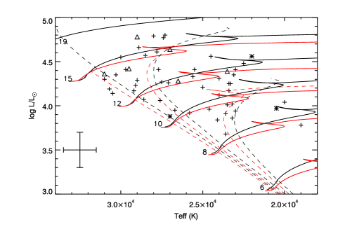
Figure 7: Observed luminosities for the VFTS sample as a function of effective temperature. Targets with an estimated nitrogen abundance, 7.2$\leq$$\epsilon_{\rm{N}}$$<$7.5 dex, are shown as asterisks and those with $\epsilon_{\rm{N}}$$\geq$7.5 dex are shown as triangles; all other targets are shown as crosses. Evolutionary tracks and isochrones (see caption to Fig. 3) are also shown, together with typical uncertainties in the effective temperatures and luminosity estimates.

In Fig. 7, the observed luminosities estimated in Sect. 2 are shown as a function of effective temperature and imply that the nitrogen enhanced stars may have larger luminosities. Indeed these stars have both higher mean observed (4.45$\pm$0.19 dex) and Bonnsai (4.47$\pm$0.22 dex) luminosities than the other targets (4.20$\pm$0.27 dex and 4.42$\pm$0.27 dex respectively). This is consistent with the differences in the masses discussed above. Student t-tests and Mann-Whitney U-tests returned probabilities that the two parent populations were the same at the $\sim$5-6% level apart from the t-test for the observed luminosities where the probability was $\sim$3%.

The lifetimes estimated by Bonnsai ranged from $\sim$0–30 Myr with there being significant uncertainties in individual values due to the samples lying close to the zero age main sequence and the age estimates thereby being very sensitive to the adopted gravity. The FLAMES-I sample have on average larger age estimates than those for the VFTS sample, which is consistent with the target selection (see Evans et al. 2006, 2011, for details). The median and average of the predicted ages of the VFTS nitrogen enriched targets (8.1 and 9.5$\pm$4.4 Myr) were lower than those for the other stars (10.9 and 12.6$\pm$7.7 Myr). Similar differences were found for the FLAMES-I sample, viz. nitrogen enhanced stars: 9.3 and 9.0$\pm$4.42 Myr; other stars: 14.0 and 14.3$\pm$8.8 Myr. However again statistical tests showed that these differences were not significant at a 5% level.

The nitrogen abundances predicted by Bonnsai ranged from 6.89–6.91 dex – in effect implying no nitrogen enhancement from the initial value of 6.89 dex adopted in the models of Brott et al. (2011a). Additionally the predicted initial and current rotational velocities were small and less than or equal to 40 km s^-1. This is consistent with the small $v_{\rm{e}}\sin i$ ($\leq$40 km s^-1) estimates of these samples and the low probability of observing targets at small angles of incidence. Indeed it qualitatively re-enforces the results presented in Sect. 6.4, which found that the numbers of observed nitrogen enhanced targets were significantly larger than predicted by our simulations.

For the nitrogen enhanced objects, Bonnsai was re-run including the estimated nitrogen abundance as a further constraint for all nine (five VFTS and four FLAMES-I) targets. In all cases, the best fitting model had both high initial ($v_{\rm{i}}$) and current ($v_{\rm{e}}$) rotational velocities, which were consistent with the adopted limits given in Table 6 to achieve significant nitrogen enhancements by rotational mixing. However for four targets (VFTS 095 and 881, NGC2004/53 and N11/100), the Bonnsai solutions failed both the posterior predictive check and a ${\mathchoice{\raisebox{1.50696pt}{$\displaystyle\chi$}}{\raisebox{1.50696pt}{$\textstyle\chi$}}{\raisebox{1.50696pt}{$\scriptstyle\chi$}}{\raisebox{1.50696pt}{$\scriptscriptstyle\chi$}}}^{2}$-test. This difficulty in finding single star evolutionary models that match the observed parameters of our nitrogen enhanced targets again re-enforces the inconsistencies discussed in Sect. 6.3.

To summarise, there is some evidence that the nitrogen enriched targets with $v_{\rm{e}}\sin i$ $\leq$ 40 km s^-1 may have higher masses, effective temperatures and luminosities, together with smaller lifetimes, assuming that they have evolved as single stars. The higher mass estimates are consistent with a previous population synthesis for the FLAMES-I B-type stars by Brott et al. (2011b) and the analysis of the evolved VFTS O-type targets by Grin et al. (2017).

6.6.2 Physical assumptions in single star evolutionary models

The discrepancy between the observed and predicted numbers of nitrogen enhanced targets discussed in Sect. 6.4 could be due to the physical assumptions adopted in the stellar evolutionary models. For example, as discussed by Grin et al. (2017), the efficiency of rotational mixing in the single-star evolutionary models of Brott et al. (2011a) was calibrated using efficiency factors based on the B-type dwarfs in the FLAMES-I survey but excluding nitrogen enhanced targets with low projected rotational velocities. Hence an increase in mixing efficiencies could in principle explain our nitrogen enriched targets. For example the five VFTS targets with nitrogen enhancements of greater than 0.6 dex and $v_{\rm{e}}\sin i$$\leq 40$ km s^-1 (see Table 7) could be reproduced by reducing the current rotational velocity, $v_{\rm{e}}$ for such an enhancement, to the unrealistically low value of $\sim$ 70 km s^-1. However this would also increase the number of nitrogen enriched targets in the 40 $<$ $v_{\rm{e}}\sin i$$\,\leq$ 80 km s^-1 cohort to $\sim$ 20 far higher than is observed. Similar arguments apply to the FLAMES-I sample where the fraction of nitrogen enhanced targets is even larger. Indeed the ratios of nitrogen enriched targets in the two projected rotational velocity cohorts provides strong evidence against the observed nitrogen enriched stars being rotationally mixed stars observed at small angles of inclination.

Another possibility is our nitrogen enriched targets may have had severe stripping of their envelopes, thereby revealing chemically enriched layers. The associated mass loss could also have removed angular momentum from the surface, resulting in spin-down. However the predicted mass loss for our targets from the Bonnsai simulations or from the grid of models of Georgy et al. (2013b) is very small (typically less than 5% of the initial mass) making such an explanation implausible.

In summary, there is no evidence that limitations on the physical assumptions made in the stellar evolutionary models can explain our nitrogen enhanced targets. Indeed the similarity of their physical properties to those of the other targets (discussed in Sect. 6.6.1) argues against such an explanation.

6.6.3 Magnetic fields in single stars

The models discussed in Sect. 6.6.1 and 6.6.2 assume that magnetic fields are unimportant for a star’s evolution. Such fields have been previously suggested as an explanation for nitrogen enriched, slowly rotating Galactic early-B stars (Morel et al. 2008; Morel 2012; Przybilla & Nieva 2011). However, more recently, Aerts et al. (2014) found no significant correlation between nitrogen abundances and magnetic field strengths in a statistical analysis of 68 Galactic O-type stars that addressed the incomplete and truncated nature of the observational data.

Meynet et al. (2011) discussed the possibility of magnetic braking (see Ud-Doula et al. 2009, and references therein) during the main-sequence phase. Models with differential rotation and magnetic braking produced strongly mixed stars with low surface rotational velocities. By contrast models with solid-body rotation and magnetic braking produce stars that at the terminal age main sequence had low surface rotational velocities and effectively no changes in the surface abundances. Potter et al. (2012a, b) have considered the $\alpha-\Omega$ dynamo as a mechanism for driving the generation of large-scale magnetic flux. They found that this mechanism was effective for stellar masses up to $\sim$15  $\rm{M}_{\odot}$ (which includes effectively all the stars in our samples). B-type main sequence stars with sufficiently high rotation rates were found to develop an active dynamo and so exhibited strong magnetic fields. They then were spun down quickly by magnetic braking and magneto-rotational turbulence (Spruit 2002) leading to enhanced surface nitrogen abundances.

Both observational and theoretical investigations have therefore led to inconclusive results about whether magnetic fields could enhance stellar mixing. However it is an attractive mechanism for explaining our nitrogen enhanced stars as it can combine both high nitrogen abundances and low stellar rotation velocities. The incidence of magnetic fields in early-type stars is currently being investigated by the MiMes survey (Wade et al. 2014, 2016) and by the BOB survey (Morel et al. 2014, 2015). The MiMes survey had a number of criteria for selecting their survey sample, one of which favoured stars with $v_{\rm{e}}\sin i$ $\leq$ 150 km s^-1. They found a frequency of 7$\pm$1% for magnetic fields in 430 B-type stars (Wade et al. 2014) with a similar frequency for O-type stars (Grunhut et al. 2017). The BOB survey have found a detection rate of 6$\pm$4% for a sample of 50 OB-type stars, while by considering only the apparently slow rotators they derived a detection rate of 8$\pm$5% (Fossati et al. 2015b). Additional observations for 28 targets led to revised estimates of 6$\pm$3% and 5$\pm$5% (Schöller et al. 2017).

These detection frequencies appear to be consistent with the percentages of nitrogen enriched targets estimated for the VFTS and FLAMES-I surveys (see Sect. 6.5). However the two magnetic surveys have necessarily only observed Galactic targets and may not be directly applicable to an LMC metallicity. Also both surveys preferentially detect targets with large magnetic fields, typically $>$100 Gauss (Morel et al. 2015). Fossati et al. (2015a) on the basis of intensive observations of two very bright stars $\beta$ CMa and $\epsilon$ CMa detected relatively weak magnetic fields and concluded that such fields might be more common in massive stars than currently observed. However the simulations of Meynet et al. (2011) for these magnetic field strengths imply that the enhancement of nitrogen occurs slowly during the hydrogen burning phase. In turn this would imply that such stars might appear to be older, which is not observed with our nitrogen enhanced targets.

Fossati et al. (2016) have estimated the fundamental parameters including ages, for a sample of 389 early-type stars, including 61 stars that have magnetic fields. The atmospheric parameters of the latter appear similar to those of the other hydrogen burning main sequence (MS) stars and they concluded that ‘the fraction of magnetic massive stars remains constant up to a fractional MS age of $\simeq$0.6 and decreases rapidly at older ages’. Hence there is no evidence for magnetic stars being older, although the rate of nitrogen enrichment would appear to depend on their magnetic field strength.

Stars with magnetic fields could account for our observed nitrogen enhanced stars and indeed this would appear to be a promising explanation. However, it should be noted that the lack of nitrogen enhanced primaries in the VFTS binary systems (Garland et al. 2017) and the existence of nitrogen enhanced targets amongst the O-type stars (see Grin et al. 2017, and references therein), where the mechanism proposed by Potter et al. (2012b) would not appear to be applicable, imply that more than one mechanism might be responsible.

6.6.4 Extant binary systems

The analysis of Dunstall et al. (2015) of the VFTS B-type sample identified targets that were members of a binary systems, both SB1 and SB2. However the remaining targets (including those with low projected rotational velocities considered here) will contain undetected binary systems. Dunstall et al. (2015) estimated that that whilst their observed binary fraction was 0.25$\pm$0.02, the true binary fraction was 0.58$\pm$0.11. In turn this implies that approximately half of the sample may in fact be binary system. These will be weighted towards long period system with periods, $P>100$ days, where the probability of detection decreases; these pre-interaction systems might be expected to evolve as single stars. However there will also be shorter period systems (often with small orbital angles of inclination) that remain undetected and these could possibly explain the nitrogen enriched objects.

Garland et al. (2017) analysed VFTS spectroscopy to estimate the atmospheric parameters of the primaries with $v_{\rm{e}}\sin i$ $<80$ km s^-1 in 33 B-type binaries. Surprisingly none of these primaries had $\epsilon_{\rm{N}}$$\geq$7.5 dex and in only one case was the upper limit consistent with such a nitrogen abundance. Indeed a preliminary comparison by Garland et al. (2017) of their results with those found here implied that their binary sample did not contain significantly nitrogen enriched binaries. They concluded that their systems were in a pre-interaction epoch and evolving as single stars with low rotational velocities and small amounts of rotational mixing (de Mink et al. 2009). Hence it would appear unlikely that the nitrogen enrichments in our sample have been produced by processes in targets that are currently pre-interaction binaries. The simulation of Dunstall et al. (2015) would then imply that if our nitrogen enriched targets are indeed single, they may make up an even larger fraction of the single B-type star cohort with $v_{e}\leq 40$ km s^-1; the actual increase would depend on the frequency of undiscovered binaries with different projected rotational velocities.

6.6.5 Post-interaction binaries

Another possible explanation of the nitrogen enhanced targets is that they are the product of binary systems in which the components have interacted. de Mink et al. (2014) discussed how such interactions could increase the fraction of stars that were classified as single on the basis of a lack of radial velocity variations. Firstly in the case of a stellar merger, the product would now be a single star. Secondly, following mass transfer, the mass gainer would dominate the light from the system (precluding an SB2 classification), whilst typically only having modest radial velocity variations (less than 20 km s^-1).

Ramírez-Agudelo et al. (2013) suggested that such a population of post-interaction binaries may explain the presence of a high-velocity tail ($v_{\rm{e}}\sin i$ $>300$ km s^-1) found in the rotational velocity distribution of the VFTS ‘single’ O-type star sample, which had been initially proposed by de Mink et al. (2013). Further support for this was the apparent absence of such a high rotational velocity tail for the pre-interacting VFTS O-type binaries analysed by Ramírez-Agudelo et al. (2015).

The possibility that the nitrogen enhanced FLAMES-I targets might be binary products was considered by Brott et al. (2011b). For example, as discussed by Langer et al. (2008), post-mass transfer systems may remain so tightly bound that tidal interaction could spin down the (observed) accreting component. However Brott et al. (2011a) concluded that ‘close binary evolution, as far as it is currently understood, is unlikely to be responsible for the slowly rotating nitrogen-rich population of observed stars’. This was based on the binary star pathways discussed by Langer et al. (2008) implying that most post-interaction objects would be rapidly rotating.

Magnetic fields could also play a role in binary systems via mergers of pre-main or main sequence stars (Schneider et al. 2016). The former could occur via tidal interactions with circumstellar material (Stahler 2010; Korntreff et al. 2012), whilst the latter would occur in some binary evolutionary pathways (Podsiadlowski et al. 1992; Langer 2012). Then the nitrogen enrichment would be due to the merger and its aftermath and/or rotational mixing of the rapidly rotating product. If the stellar merger also produced a magnetic field, this could then be an efficiently spin down mechanism. Products of stellar mergers may represent $\sim$10% of the O-type field population (de Mink et al. 2014). If mergers represented a similar fraction of the B-type population, this would be consistent with the percentages of nitrogen enriched stars discussed in Sect. 6.5. Additionally the products of such mergers might be expected to be more massive and appear younger than other single B-type stars. Tentative evidence for this can be seen in Fig. 3 and 7 and has been discussed in Sect. 6.6.1.

In summary, post-interaction binary evolutionary pathways are available that might produce slowly rotating, nitrogen enriched, apparently single stars, either by mass transfer or mergers. The latter would also be consistent with the masses and ages inferred for our stellar samples. However models exploring the wide variety of possible evolutionary pathways are required for further progress to be made.

7 Conclusions

Our principle conclusions are that:

1. Approximately 75% of the targets in the FLAMES-I and VFTS surveys with $v_{\rm{e}}\sin i$ $\leq$ 80 km s^-1 have nitrogen enhancements of less than 0.3 dex. As such they would appear to be slowly rotating stars that have not undergone significant mixing.

2. Both surveys contain stars that exhibit significant nitrogen enhancements. The relative numbers in the cohorts with projected rotational velocities, $v_{\rm{e}}\sin i$ of 0–40 km s^-1 and 40–80 km s^-1 are inconsistent with these being rapidly rotating stars observed at small angles of inclination.

3. For both surveys, the number of targets with $v_{\rm{e}}\sin i$ $\leq$ 40 km s^-1  and $\epsilon_{\rm{N}}$ $\geq$ 7.5 dex is larger than predicted. These differences are significant at a high level of probability.

4. The percentage of these highly nitrogen enhanced objects that cannot be explained by rotational mixing are estimated to be $\sim$20-30% of single stars with current rotational velocities of less than 40 km s^-1and $\sim$2-4% of the total non-supergiant single B-type population. Given the conservative assumptions adopted in the simulations and the large nitrogen enhancements observed, these constitute robust lower limits for stars that appear inconsistent with current grids of single star evolutionary models incorporating rotational mixing.

5. Including targets with smaller nitrogen enhancements and adopting evolutionary models consistent with the median gravities and masses of our samples leads to larger estimates of the fractions of targets that are inconsistent with current evolutionary models, viz. $\sim$70% with current rotational velocities less than 40 km s^-1 and $\sim$6-8% of the total single B-type stellar population.

6. The highly nitrogen enriched targets may have higher effective temperatures, masses and luminosities than the other stars. Additionally single star evolutionary models imply that they would be younger, implying that they may be re-juvenated. However these differences are generally not significant at the 5% level.

7. Some of our targets will be undetected binaries as discussed by Dunstall et al. (2015) and this binary population does not appear to contain highly nitrogen enhanced targets (Garland et al. 2017). Hence the percentages of truly single stars that have significant nitrogen abundances may be higher than has been estimated. Indeed it is possible that effectively all the single B-type population with a current rotational velocity, $v_{\rm{e}}$$\leq$40 km s^-1 may have nitrogen abundances that are inconsistent with single star evolutionary models.

8. Possible explanations for these nitrogen enhancements are considered of which the most promising would appear to be breaking due to magnetic fields or stellar mergers with subsequent magnetic braking. The latter would be consistent with the higher masses that may pertain in the nitrogen enriched sample.