A HARDCORE model for constraining an exoplanet’s core size

Abstract

The interior structure of an exoplanet is hidden from direct view yet likely plays a crucial role in influencing the habitability of Earth analogs. Inferences of the interior structure are impeded by a fundamental degeneracy that exists between any model comprising of more than two layers and observations constraining just two bulk parameters: mass and radius. In this work, we show that although the inverse problem is indeed degenerate, there exists two boundary conditions that enables one to infer the minimum and maximum core radius fraction, $\mathrm{CRF}_{\mathrm{min}}$ & $\mathrm{CRF}_{\mathrm{max}}$. These hold true even for planets with light volatile envelopes, but require the planet to be fully differentiated and that layers denser than iron are forbidden. With both bounds in hand, a marginal CRF can also be inferred by sampling inbetween. After validating on the Earth, we apply our method to Kepler-36b and measure $\mathrm{CRF}_{\mathrm{min}}=(0.50\pm 0.07)$, $\mathrm{CRF}_{\mathrm{max}}=(0.78\pm 0.02)$ and $\mathrm{CRF}_{\mathrm{marg}}=(0.64\pm 0.11)$, broadly consistent with the Earth’s true CRF value of 0.55. We apply our method to a suite of hypothetical measurements of synthetic planets to serve as a sensitivity analysis. We find that $\mathrm{CRF}_{\mathrm{min}}$ & $\mathrm{CRF}_{\mathrm{max}}$ have recovered uncertainties proportional to the relative error on the planetary density, but $\mathrm{CRF}_{\mathrm{marg}}$ saturates to between 0.03 to 0.16 once $(\Delta\rho/\rho)$ drops below 1-2%. This implies that mass and radius alone cannot provide any better constraints on internal composition once bulk density constraints hit around a percent, providing a clear target for observers.

1 Introduction

Despite recent strides in our ability to characterize exoplanets (Kaltenegger, 2017), knowledge regarding the internal structure of distant worlds remains almost entirely lacking (Spiegel et al., 2013; Baraffe et al., 2014). Unlike the search for exoplanetary atmospheres (Burrows, 2014), moons (Kipping, 2014) or tomography (McTier & Kipping, 2017), our remote observations do not have direct access to that which we seek to infer - the planet’s interior. The habitability of an Earth-like planet, in particular via the likelihood of plate tectonics, is likely strongly influenced by the internal structure (Noak et al., 2014) and thus the community is strongly motivated to infer what lies beneath, as part of the broader goal of understanding our own planet’s uniqueness.

In general, the only information we have about an exoplanet which is directly affected by internal structure is the bulk mass and radius of the planet. Aside from this, we highlight that there are some special cases where additional information about the planetary interior can become available. For example, Kaltenegger (2010) argue that volcanism and planetary outgassing could be detectable using atmospheric characterization techniques. Certain dynamical configurations of planetary systems, such as tidal fixed points (Batygin et al., 2009) for example, can also enable inference of the planetary tidal properties, which in turn constrains internal composition (see also Kramm et al. 2012). Finally, direct measurements of oblateness may also provide constraints on internal structure (Seager & Hui, 2002; Carter & Winn, 2010; Zhu et al., 2014).

Whilst there is some hope of identifying outgassing of exoplanets, providing clues to the mantle composition (Kaltenegger, 2010), and measuring tidal dissipation constants in special cases (Batygin et al., 2009), full structure inference will likely be limited to indirect methods based on theoretical models. In this approach, one takes the basic observables we do have access to, in particular planetary mass and radius, and compares them to theoretical models in an effort to find families of compatible solutions. Since theoretical models depend on more than just two parameters, accounting for factors such as chemical composition (Valencia et al., 2006; Seager et al., 2007), ultraviolet environment (Lopez & Fortney, 2013; Batygin & Stevenson, 2013) and age (Fortney et al., 2011), the problem is degenerate, in a general sense.

Since we do not have direct access to the interior of exoplanets, their interior structure is generally modelled by assuming several key chemical constituents. In the case of solid exoplanets, extrapolation from the Solar System implies that they should be comprised of three primary chemical ingredients, namely water, H₂O, enstatite, MgSiO₃, and iron, Fe (Valencia et al., 2006). If we assume the planet is not young and has thus become fully differentiated, the equations of state of these three layers can be solved to provide theoretical estimates of the mass and radius of solid bodies (Zeng & Sasselov, 2013). A fourth layer describing a light volatile envelope can be placed on top to capture the behavior of mini-Neptunes, where the light envelope is assumed to have negligible relative mass and thus only affects the bulk radius and not the mass (Kipping et al., 2013; Lopez & Fortney, 2014; Wolfgang et al., 2016).

These four constituents can be combined in multiple ways to re-create the same mass and radius. Even in the absence of a volatile envelope this degeneracy persists, leading to the common use of ternary diagrams to illustrate their symplectic yet degenerate loci of solutions (e.g. see Seager et al. 2007). This degeneracy is a major barrier to inferring unique solutions for planetary interiors, leading authors to either switch out to simpler and non-degenerate two-layer models (e.g. Zeng et al. 2016) or adding a chemical proxy from the parent star (e.g. Dorn et al. 2017) to break the degeneracy. Whilst these are both certainly promising avenues for tackling interior inference, in this work we focus on a third approach based on boundary conditions.

The possibility of exploiting boundary conditions was first highlighted in Kipping et al. (2013), where the authors focused on the concept of “minimum atmospheric height”. The method works by first predicting the maximum allowed radius of a planet without any extended envelope given its measured mass. This atmosphere-less planet is typically assumed to be a pure water/icy body, for which detailed models are widely available. If the observed radius exceeds this maximum limit, then some finite volume of atmosphere must sit on top of the planetary interior, and the difference in radii represents the “minimum atmospheric height” (MAH). The approach therefore formally describes a key boundary condition of a general four-layer exoplanet.

In this work, we explore the other extreme, asking the question under what conditions would an observed mass and radius definitively prove some finite iron-core must exist, and what is the minimum radius fraction that the core must comprise? Going further, we argue that the maximum core radius fraction is another boundary condition in the problem and thus can be derived to provide a complete bounding box of a planet’s core size in a general four-layer model framework.

We introduce the concept of the minimum core size in Section 2, as well as our fast parametric model to interpolate the Zeng & Sasselov (2013) grid models. Section 3 discusses our approach to inverting the relation to solve for core radius fraction directly, as well as the much more straightforward method for inferring the maximum core size. In Section 4, we demonstrate the approach on both synthetic and real exoplanets, with special attention to sensitivity. Finally, we discuss the anticipated value of this work, as well its limitations, in Section 5.

2 Boundary Conditions on the Core

2.1 Outline and Assumptions

Exoplanets are generally expected to display a diverse range of physical characteristics, owing to their presumably distinct formation mechanisms, chemical environments and histories, as three examples. Even if the mass and radius of an exoplanet were known to infinite precision, and the body was known to be definitively solid, these two observed parameters are insufficient to provide a unique solution for the relative fractions of water, silicate and iron typically assumed to represent the major constituents of solid planets (Kipping et al., 2013). In other words, mass and radius alone cannot confidently reveal an exoplanet’s CRF or CMF (core radius fraction or core mass fraction, respectively).

As a concrete example, a planet composed of water and iron can have the same mass and radius as an iron-silicon planet, and thus have very different CRFs (as illustrated in Figure 1).

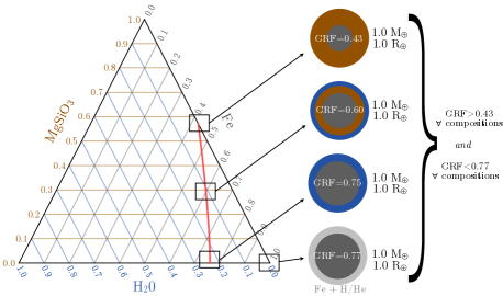
Figure 1: Ternary diagram of a three-layer interior structure model for a solid planet. All points along the red line lead to a $M=1$ $M_{\odot}$ and $R=1$ $R_{\odot}$ planet. Although indistinguishable from each other with current observations, all points satisfy having a core-radius fraction exceeding 43%, a boundary condition we exploit in this work. The largest iron core size allowed is depicted by the lowest sphere, where the volatile envelope contributes negligible mass.

As touched on in Section 1, four-layer theoretical models of solid planets are degenerate for a single mass-radius observation. However, across the suite of loci able to serve as viable solutions, there exists a boundary condition when the composition is pure silicate and iron. At this point, the CRF takes the smallest value out of all possible models, since the second-layer (the mantle) is now as heavy as it can be, being pure silicate (the second densest material). Therefore, for any given mass-radius pair, we can solve for the corresponding CRF of a pure silicate-iron model (which is not a degenerate problem) and define that this CRF must equal the minimum CRF, $\mathrm{CRF}_{\mathrm{min}}$, allowed across all models.

Similarly, another boundary condition we can exploit is to consider the maximum allowed core size. As depicted in Figure 1, this occurs when all of the mass is located within a pure iron core, padded by a second layer of a light volatile envelope. The core can’t possibly exceed this fractional size else the mass would be incompatible with the observed value.

Note that although we refer to CRF rather than CMF here and in what follows, once armed with a CRF, the mass and radius, it is easy to convert back to CMF. Note too that here and throughout in what follows, we refer to the CRF strictly in terms of an iron core. Although technically we acknowledge that a water-silicate body could be described as having a finite sized silicate core, that core would not qualify as being a “core” in this work.

Before continuing, we highlight some key assumptions of our model, for the sake of transparency:

• The planet is fully differentiated and is not recently formed.

• The outer volatile envelope has insufficient mass and thus gravitational pressure to significantly affect the equation-of-state of the inner layers.

• The densest core permitted is that of iron i.e. heavy-element (e.g. uranium) cores are forbidden.

• We have accurate models for a planet’s mass and radius given a particular compositional mix.

We stress that what has been described thus far includes the possibility of a light volatile envelope, and is not limited to some special case of two- or three-layer conditions, as discussed earlier.

Under these assumptions, the limiting core radii fractions should be determinable, although violating any of the assumptions listed above would invalidate our argument. An obvious one is that the theoretical models used are invalid or inaccurate, for example because their assumed equations of state are wrong. In this work, we primarily use the Zeng & Sasselov (2013) model but we point out that should a user believe an alternative model to be superior, it is straight-forward to reproduce the methods described in this paper using the model of their preference. The actual existence of a boundary condition remains true.

Another more serious flaw would be if the planetary body in question has a significant mineral fraction based on some heavier element than iron, for example a uranium core. Such a body could feasibly have a significantly smaller core than that derived using our approach. If evidence for such cores emerges in the coming years, then we advice against users employing the model described in this work.

The remaining two assumptions, a differentiated, non-young planet and a light volatile envelope, mean that young systems are not suitable and gas giants would not be either. In general then, the model described is expected to be valid for most planets smaller than mini-Neptunes.

2.2 A parametric interpolative model for $\mathrm{CRF}_{\mathrm{min}}$

For any combination of mass and radius, we need to be able to predict what the corresponding CRF would be for a silicate-iron two-layer model, in order to determine $\mathrm{CRF}_{\mathrm{min}}$. Inferring $\mathrm{CRF}_{\mathrm{max}}$ is far simpler and is briefly explained later in Section 2.3. In what follows, we use the models of Zeng & Sasselov (2013), which are made available as a regular grid of theoretical points. Whilst we could simply perform a nearest neighbor look-up, this is unsatisfactory since our precision will be limited to the grid spacing and resulting posteriors would be rasterized to the same grid resolution. Instead, we seek a means to perform an interpolation of the grid.

The first successful literature interpolation of the Zeng & Sasselov (2013) models comes from Kipping et al. (2013), who found that for a specific fixed CRF, each of the various two-layer models of Zeng & Sasselov (2013) are very well-approximated by a seventh-order polynomial of radius with respect to the logarithm of mass, given by

$$\frac{R}{R_{\oplus}}=\sum_{i=0}^{7}a_{i}(CRF)\times\log\Big{(}\frac{M}{M_{\oplus}}\Big{)}^{i}$$ (1)

Temperature does not feature in this expression, as Zeng & Sasselov (2013) find its effects on the density profile are secondary compared to pressure and can be safely ignored. Equation 1 is attractive since it is parametric, linear (and thus can be trained using linear least squares) and extremely fast to execute as an interpolative model once the coefficients have been assigned. Accordingly, we are motivated to pursue a similar strategy in what follows.

Consider first the mass-radius relation for a 100% silicate planet. Plotting the radius against the logarithm of the mass indeed reveals a series of points that are well described by a seventh-order polynomial, as shown in Figure 2. We found that the range for which this interpolation works best is $M>0.1$ $M_{\oplus}$ and thus we set this as a truncation point during training. Note that any planet that lies beneath this polynomial curve must have an iron core.

However, our goal is to not only determine whether or not a planet has an iron core, but also quantify the minimum CRF. To accomplish this, we trained a suite of seventh-order polynomials on models with varying CRFs assuming the two-layer iron-silicate models of Zeng & Sasselov (2013). We varied the CRF from 0 to 1 in 0.025 steps and perform a linear least squares regression at each step. To illustrate this, a gradient of interpolations of the mass-radius relation for the CRFs between 0 and 1 are shown in Figure 3.

In order to have a general model, we are interested in parameterizing the CRF variable to understand the relation of the polynomials shown in Figure 3. To do this, we allow the coefficients of the polynomials to be polynomials themselves (but with respect to CRF rather than logarithmic mass), such that

$$a_{i}(CRF)=\sum_{j=0}^{M_{i}}b_{i,j}\mathrm{CRF}^{j},$$ (2)

where $M_{i}$ is the polynomial order of the $i^{\mathrm{th}}$ coefficient and $b_{i,j}$ is the $j^{\mathrm{th}}$ “sub-coefficient” of the the $i^{\mathrm{th}}$ coefficient.

As an example, in the case of the $a_{0}$ coefficient, we first graphed the coefficient for 40 steps as a function of the corresponding CRF (see top-left panel of Figure 4). It was immediately apparent that the points followed a smooth function that could be stably approximated by another polynomial. The polynomial-order was initially third-order and then we stepped through until the polynomial appeared to go through almost all of the data, ranging from fifth to tenth order. The same process was repeated for the remaining eight coefficients. The resulting functions are presented in Figure 4, with the coefficients tabulated in Table 1.

Table 1: Coefficients for the terms in Equation 2. These are implemented in our package HARDCORE available at this URL.

j	$b_{0,j}$	$b_{1,j}$	$b_{2,j}$	$b_{3,j}$	$b_{4,j}$	$b_{5,j}$	$b_{6,j}$	$b_{7,j}$
0	1.042859	0.717298	0.203201	0.015509	-0.009827	-0.004411	-0.000811	-0.000058
1	-0.022816	-0.024719	-0.001194	-0.000338	-0.001129	0.000238	0.000025	0.000002
2	0.246925	0.292204	0.012756	0.017228	0.018847	-0.004520	0.000727	-0.000002
3	-1.525749	-1.703841	-0.076864	-0.378486	-0.175492	0.031420	0.021119	0.001470
4	1.436881	1.827627	-1.346393	2.642471	0.599478	-0.033670	-0.150980	-0.010296
5	-0.406604	-0.606841	3.407122	-13.375869	-0.886996	-0.009464	0.712172	0.048466
6	0	0	-2.951612	39.839020	0.614844	0.028879	-2.038051	-0.142873
7	0	0	0.884763	-67.898807	-0.165447	-0.010646	3.449051	0.249493
8	0	0	0	66.023432	0	0	-3.387940	-0.251336
9	0	0	0	-34.234323	0	0	1.788366	0.135208
10	0	0	0	7.358617	0	0	-0.392564	-0.030096

To validate our model, we re-trained our model of all of the original training data Zeng & Sasselov (2013) but omitting a random single datum each time, serving as a hold-out validation point. We then computed the relative difference between the prediction for that point using the re-trained model, and the actual value. Repeating for $10^{4}$ random hold-out points, we find that the mean error of our model is 0.045% and the maximum error is 0.24%.

To assist the community, we make our model, which we dub HARDCORE, publicly available at this URL.

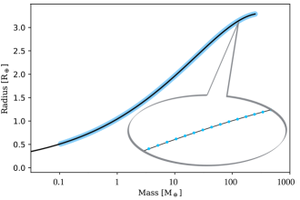
Figure 2: Theoretical mass-radius grid points of a pure silicate planet from Zeng & Sasselov (2013), shown in blue. For comparison, we show our $7^{\mathrm{th}}$ order polynomial fit. We only recommend this interpolation for masses above 0.1 $M_{\oplus}$.

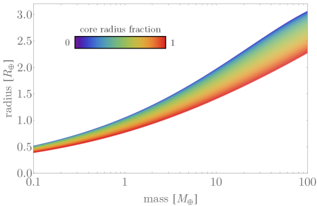
Figure 3: Interpolated theoretical mass-radius relations for a silicate-iron two-layer solid planet for various core radius fractions (CRFs), based off Zeng & Sasselov (2013). All interpolations for CRFs between 0 and 1 are seventh-order polynomials. We are then motivated to describe the dependence of the polynomials with respect to the CRF, by making the these coefficients polynomial functions themselves.

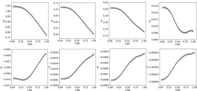
Figure 4: Interpolated functions for the coefficients of seventh-order polynomials. Given a specific CRF, one can use this parameterization to solve for all eight coefficients, to then use for a seventh-order polynomial. This seventh order polynomial can then describe the mass-radius function corresponding to all CRFs, not just the ones tabulated by Zeng & Sasselov (2013).

2.3 A parametric model for $\mathrm{CRF}_{\mathrm{max}}$

Determining $\mathrm{CRF}_{\mathrm{max}}$ is far more straight-forward than $\mathrm{CRF}_{\mathrm{min}}$. One may simply take the 100% iron mass-radius models, in our case from Zeng & Sasselov (2013), and directly compute the expected radius of a pure iron planet given an observed mass, $R_{\mathrm{iron}}(M_{\mathrm{obs}})$.

The maximum core radius fraction is then easily computed as $\mathrm{CRF}_{\mathrm{max}}=R_{\mathrm{iron}}(M_{\mathrm{obs}})/R_{\mathrm{obs}}$. In practice, this inversion is far simpler than $\mathrm{CRF}_{\mathrm{min}}$ since we need not interpolate across intermediate mixtures of iron and silicate compositions, but rather cam simply directly solve for $\mathrm{CRF}_{\mathrm{max}}$ if an analytic expression for $R_{\mathrm{iron}}(M)$ is available. This could be estimated using our interpolative model but is more directly accessible by simply fitting Equation 1 to the Zeng & Sasselov (2013) grid for the specific points corresponding to a pure iron composition, which were previously presented in the final column of Table 1 of Kipping et al. (2013).

3 Solving for the CRF Limits

3.1 From forward- to inverse-modeling

Thus far we have described a method to solve for $\mathrm{CRF}_{\mathrm{max}}$ but not for $\mathrm{CRF}_{\mathrm{min}}$. The silicate-iron interpolative model is a forward model in which we begin with knowledge of both the planet’s mass and minimum core radius fraction and compute the corresponding radius. In practice, however, we are interested in the inverse model, where we wish to determine $\mathrm{CRF}_{\mathrm{min}}$ from the mass and radius.

The nested coefficient structure makes the problem non-linear with respect to $\mathrm{CRF}_{\mathrm{min}}$, yet it is one dimensional and found to be unimodal in practice. For these reasons, it is amenable to a large number of possible optimization algorithms, but in what follows we adopted Newton’s method, since we are able to directly differentiate our functions thanks to their parametric nature.

Specifically, in our implementation we minimize the following cost function, $J$, with respect to one degree of freedom, the $\mathrm{CRF}$:

$$J =(R_{\mathrm{Fe-Si}}(\mathrm{CRF};M_{\mathrm{obs}})-R_{\mathrm{obs}})^{2},$$ (3)

where $M_{\mathrm{obs}}$ and $R_{\mathrm{obs}}$ are the observed mass and radius of the planet, and $R_{\mathrm{Fe-Si}}(\mathrm{CRF};M)$ is the radius of a two-layer iron + silicate model with core radius fraction $\mathrm{CRF}$ and mass $M$. The latter function is determined using the smooth parametric interpolation model described in Section 2.2. Our inversion algorithm, starts at an initial guess of $\mathrm{CRF}_{\mathrm{min}}=0.5$ and then iterates by computing

$$\mathrm{CRF}_{i+1} =\mathrm{CRF}_{i}-\frac{J(\mathrm{CRF}_{i})}{[\mathrm{d}J/\mathrm{d}\mathrm{CRF}](\mathrm{CRF}_{i})}.$$ (4)

To improve speed and stability, we impose a check as to whether $R_{\mathrm{obs}}$ is below that of a pure iron planet of mass $M_{\mathrm{obs}}$, in which case we fix $\mathrm{CRF}_{\mathrm{min}}=1$, or if the radius exceeds that of an pure silicate planet of mass $M_{\mathrm{obs}}$ (where again we use the interpolative model of Kipping et al. 2013), in which case we fix $\mathrm{CRF}_{\mathrm{min}}=0$.

3.2 The Earth as an example

Let us use the Earth itself as an example of our method. We took a 1 $M_{\oplus}$ and $1$ $R_{\oplus}$ planet and used the methods described earlier to solve for $\mathrm{CRF}_{\mathrm{min}}$ and $\mathrm{CRF}_{\mathrm{max}}$, giving $\mathrm{CRF}_{\mathrm{min}}=0.43$ and $\mathrm{CRF}_{\mathrm{max}}=0.77$.

In reality, the Earth is not perfectly described by the Zeng & Sasselov (2013) model and the core in particular is only $\sim 80$% iron, with nickel and other heavy elements comprising the rest. The mantle-core boundary occurs at a radius of 3480 km relative to the Earth’s mean radius of 6371 km (Dziewonski & Anderson, 1981), meaning that its actual $\mathrm{CRF}=0.55$. Accordingly, our CRF bounds correctly bracket the true solution, as expected.

We go further by treating these limits as being bounds on a prior distribution for CRF. Adopting the least informative continuous distribution for a parameter constrained by only two limits corresponds to a uniform distribution. Sampling from said distribution yields a marginalized CRF of $\mathrm{CRF}_{\mathrm{marg}}=0.600\pm 0.098$, which is again fully compatible with the true value.

To test our inversions in a probabilistic sense, we decided to create a mock posterior distribution of an Earth-like planet where $M\sim\mathcal{N}[1.0M_{\oplus},0.01M_{\oplus}]$ and $R\sim\mathcal{N}[1.0R_{\oplus},0.01R_{\oplus}]$ (we also apply a truncation to the distributions at zero to prevent negative masses/radii). This is clearly an optimistic assumption but a more detailed investigation of sensitivity for different relative errors is tackled later in Section 3.3. Generating $10^{5}$ samples, we inverted each sample as described earlier to produce a posterior for $\mathrm{CRF}_{\mathrm{min}}$ and $\mathrm{CRF}_{\mathrm{max}}$. Our experiment returns near-Gaussian like distributions for both terms with a mean and standard deviation given by $\mathrm{CRF}_{\mathrm{min}}=(0.43\pm 0.04)$ and $\mathrm{CRF}_{\mathrm{max}}=(0.7716\pm 0.0080)$. This establishes that the inversions are stable against perturbations around physical solutions.

As a brief aside, we argued earlier in Section 2.1 that the principle of exploiting the boundary condition of theoretical models to infer $\mathrm{CRF}_{\mathrm{min}}$ does not explicitly require solid planets and works for mini-Neptunes too. To demonstrate this point with a specific example, let us return to the earlier thought experiment of the Earth as a gaseous planet consisting of a solid iron core surrounded by a light H/He envelope. We consider that the mass and radius of the planet remain the same as the real Earth, and that the envelope significantly influences the radius but has negligible mass. Using the 100% iron-model of Zeng & Sasselov (2013) and the corresponding $7^{\mathrm{th}}$ order polynomial interpolation of Kipping et al. (2013), we estimate that a 1 $M_{\oplus}$ iron core would have a radius of 0.77 $R_{\oplus}$ and therefore the remaining 0.23 $R_{\oplus}$ is given by the light, H/He envelope as depicted earlier in Figure 1. Accordingly, such a body would have a core radius fraction exceeding our inferred minimum value of $\mathrm{CRF}$ (which was $\mathrm{CRF}>0.43$), which is expected and self-consistent with our definition of $\mathrm{CRF}_{\mathrm{min}}$.

We highlight that the counter-example described above is highly unphysical though; $1$ $R_{\oplus}$ are not expected to retain significant volatile envelopes in mature systems, both from a theoretical perspective (Lopez & Fortney, 2014; Owen & Wu, 2017) and an observational one (Rogers, 2015; Chen & Kipping, 2017; Fulton et al., 2017).

3.3 Sensitivity analysis for an Earth

A basic and important question to ask is what kind of precisions on a planet’s mass and radius lead to meaningful constraints on $\mathrm{CRF}_{\mathrm{min}}$? In other words, what is the correspondence we might expect between $\{(\Delta M/M),(\Delta R/R)\}$ and $(\Delta\mathrm{CRF}_{\mathrm{min}}/\mathrm{CRF}_{\mathrm{min}})$? This is key for designing future observational surveys, where primary science objectives may center around inferring internal compositions. To investigate this, we repeated the retrieval experiment described in Section 3.2, but varied the fractional error on mass and radius away from the fixed 1% value previously assumed.

In total, we generated $81^{2}=6561$ experiments, where for each one we generated a new mock posterior of $10^{5}$ mass-radius samples, which was then converted into a posterior of $\mathrm{CRF}_{\mathrm{min}}$ and $\mathrm{CRF}_{\mathrm{max}}$. For each experiment, we record the standard deviation of the resulting posteriors as $\Delta\mathrm{CRF}_{\mathrm{min}}$ and $\Delta\mathrm{CRF}_{\mathrm{max}}$. The errors on the mass and radius were independently varied with a fractional error given by $10^{x}$, where $x$ was varied across a regular grid from -4 to $0$ in 0.05 steps, giving 81 grid points in each dimension, and thus 6561 across both. In all experiments, the underlying mass and radius posteriors are generated assuming a mean of $\mu_{M}=1$ $M_{\oplus}$ and $\mu_{R}=1$ $R_{\oplus}$.

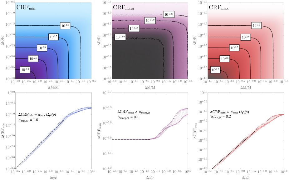
Figure 5: Upper: Contour plots depicting the a-posteriori standard deviation on the minimum (left), marginalized (center) and maximum (right) CRF, as a function of the fractional errors on mass and radius. Lower: Re-parameterization of the above plots by combining the mass and radius axes into a single density term, demonstrating a strong dependency in all cases.

Figure 5 displays the results of this effort for each combination of mass and radius error. Given the shape of darker areas of the color plot, one can see that radius is the dominant constraint, and that for the same fractional error on mass and radius, it is the radius term which mostly strongly constrains $\mathrm{CRF}_{\mathrm{min}}$. For example, we find that in order to obtain a precision of 10% on $\mathrm{CRF}_{\mathrm{min}}$, we require a measurement on the mass better than 11% and a measurement on the radius better than 3%.

The ratio of these two numbers, close to three-to-one, led to us hypothesize that density was the underlying driving term. This can be seen by calculating error on density for independent mass and radius via

$$\frac{\Delta\rho}{\rho} =\frac{\Delta M}{M}+3\frac{\Delta R}{R}.$$ (5)

This is verified in the lower panels of Figure 5, where we find that although density doesn’t perfectly capture the dependency, it describes the vast majority of the variance. For precise densities ($\lesssim 1$%), the dependency is strictly linear where we give the coefficients in the panels. This linear dependency breaks down as the errors grow, likely as a result of the truncated normals used to generate the masses and radii becoming increasingly skewed and the finite support interval (zero to unity) of the CRF itself causing a saturation effect.

The marginalized CRF behaves quite different to the other two. The upper-central panel of Figure 5 alone looks fairly consistent with the previous, just with inflated errors. This is to be expected by the very act of marginalization. However, the bottom-central panel does not exhibit a simple linear dependency, even at precise densities. In contrast, at precise densities the marginalized CRF appears to saturate to ${\sim}10$%. This implies that no better than 10% precision can ever be obtained on the $\mathrm{CRF}$ using just mass and radius alone.

3.4 Generalized sensitivity analysis

Thus far, we have assumed a $M=1$ $M_{\oplus}$, $R=1$ $R_{\oplus}$ planet. In order to generalize the scalings found, we decided to vary these inputs and repeat the entire process described above. We varied the mass from 1 to 10 Earth masses logarithmically and the CRF from 0.2 to 0.8 uniformly, exploring over 1000 different realizations. For the $\mathrm{CRF}_{\mathrm{max}}$ term, we find that

$$\Delta\mathrm{CRF}_{\mathrm{max}} \simeq\alpha_{\mathrm{max}}\Bigg{(}\frac{\Delta\rho}{\rho}\Bigg{)}$$ (6)

provides an excellent fit across all simulations, where the best-fitting value of the coefficient term ranged from $0.187<\alpha_{\mathrm{max}}<0.237$. The relationship is sufficiently tight that it is reasonable to simply adopt $\alpha_{\mathrm{max}}\simeq 0.2$ as a general rule of thumb. Repeating for the minimum limit on the CRF we find that the function

$$\Delta\mathrm{CRF}_{\mathrm{min}} \simeq\alpha_{\mathrm{min}}\Bigg{(}\frac{\Delta\rho}{\rho}\Bigg{)}$$ (7)

again provides excellent fits, but now the coefficient term varies dramatically from $0.6<\alpha_{\mathrm{min}}<4$ across all simulations, or logarithmically a range of $-0.3<\log_{10}\alpha_{\mathrm{min}}<0.66$. The behaviour of $\alpha_{\mathrm{max}}$ appears to display a peculiar and periodic dependency with respect to the dependent variables, CRF and mass. We were unable to identify a simple physically motivated relation after substituting for terms such as density and surface gravity, but were able to capture the most of the variance using an empirical approximate formula given by

$$\log_{10}\alpha_{\mathrm{min}}\simeq-0.340985+0.0766358\mathrm{exp}\beta_{\mathrm{min}},$$ (8)

where

$$\beta_{\mathrm{min}}\simeq \lfloor 4.934(\mathrm{CRF}-\tfrac{8}{3}\log_{10}M-\tfrac{2}{3}\mathcal{R}[1.34-4\log_{10}M]\rfloor$$

$$-3.28933\mathcal{R}[4(\log_{10}M-0.335)]-4.934\mathrm{CRF}$$

$$+13.1573\log_{10}M.$$ (9)

where $\mathcal{R}$ is a rounding function. We find the above function has a robust (via the median absolute deviation) estimate of the RMS in the residuals of $\Delta(\log_{10}\alpha_{\mathrm{min}})=0.058$.

The marginal CRF plateau, which was 10% in the case of the Earth, also varies in a non-trivial manner, ranging from 2.8% to 15.7% across our suite of simulations. Fortunately, the location of the plateau appears to be directly related to $\alpha_{\mathrm{min}}$, and thus we can use our earlier empirical function to predict this term too with

$$\Delta\mathrm{CRF}_{\mathrm{marg}} \simeq\alpha_{\mathrm{marg}}$$ (10)

where

$$\log_{10}\alpha_{\mathrm{marg}}\simeq -0.9819-0.00583\mathrm{exp}(-13.6\log_{10}\alpha_{\mathrm{min}})$$

$$+0.321\log_{10}\alpha_{\mathrm{marg}}.$$ (11)

We briefly comment that this saturation-behavior can be understood as follows. With imprecise data, the posteriors on the minimum and maximum limits will be broad, and so sampling a point between them will yield an even broader distribution. As the data become more precise, the posteriors distributions for $\mathrm{CRF}_{\mathrm{min}}$ and $\mathrm{CRF}_{\mathrm{max}}$ converge towards sharp delta functions, but these two limits have no reason or expectation to be on top of one another. Accordingly, when we draw samples between them uniformly, we will still get a broad distribution, albeit one less broad than that obtained when $\mathrm{CRF}_{\mathrm{min}}$ and $\mathrm{CRF}_{\mathrm{max}}$ were also broad.

4 Example Application

To demonstrate the value of our prescription, we show here an example application to a real exoplanetary system. As established in Section 3.3, precise measurement errors on both planetary mass and radius are required in order to infer $\mathrm{CRF}_{\mathrm{min}}$ at a meaningful level, certainly better than 10% on both.

One of the best laboratories for precise measurements of planetary properties comes from dynamically interacting systems, particularly those in near mean motion resonances (MMRs) where transit timing variations (TTVs) may strongly constrain planetary mass (Holman & Murray, 2005; Agol et al., 2015). A good example comes from the Kepler-36 system, where two planets gravitationally perturb one another, enabling a measurement of both masses to better than 8% precision (Carter et al., 2012). Coupled with precise planetary radii at precisions better than 2.5%, and the low-radius, high-density nature of Kepler-36b in particular ($R_{b}=(1.486\pm 0.035)$ $R_{\oplus}$ and $\rho_{b}=7.45_{-0.59}^{+0.74}$ g cm^-3), Kepler-36 offers an excellent test case for our technique.

To implement our code, we follow a similar procedure to that used in Section 3.2, except that we now use the real mass-radius joint posterior distribution of Kepler-36b derived by Carter et al. (2012), which features $10^{4}$ independent samples. Kepler-36c was not used as the planet more likely resembles a gas giant than a terrestrial body, as established using the MAH technique in Kipping et al. (2013), who find that a volatile envelope comprises at least 36% of Kepler-36c’s bulk radius.

The resulting posterior distributions on the $\mathrm{CRF}_{\mathrm{min}}$ and $\mathrm{CRF}_{\mathrm{max}}$ for Kepler-36b are shown in Figure 6. The $\mathrm{CRF}_{\mathrm{min}}$ posterior indicates strong evidence for the presence of an iron core with $\mathrm{CRF}_{\mathrm{min}}=0.497_{-0.074}^{+0.067}$. We obtain a tighter constraint on $\mathrm{CRF}_{\mathrm{max}}$, as predicted by our earlier sensitivity analysis, of $\mathrm{CRF}_{\mathrm{max}}=0.777\pm 0.020$, which is exactly what would be predicted from our scaling expression in Equation 6 for a 10% error on the planet’s bulk density, which is indeed approximately the reported value.

By drawing random samples between $\mathrm{CRF}_{\mathrm{min}}$ and $\mathrm{CRF}_{\mathrm{max}}$ on a sample by sample basis, we can construct the $\mathrm{CRF}_{\mathrm{marg}}$ posterior, revealing that $\mathrm{CRF}_{\mathrm{marg}}=0.64\pm 0.10$. Given that the fractional density error exceeds ${\sim}10^{-1.5}$, this precision does not lie on the sensitivity plateau depicted in Figure 5, and therefore we predict that the precision on Kepler-36b’s $\mathrm{CRF}_{\mathrm{marg}}$ could be improved. Since Carter et al. (2012) only considered ten quarters, it should be possible to considerably improve the uncertainties by re-analyzing the entire Kepler time series.

For comparison, the Earth’s $\mathrm{CRF}$ is 0.55 but inverting $\mathrm{CRF}_{\mathrm{marg}}$ for a synthetic Earth yields $\mathrm{CRF}_{\mathrm{marg}}=0.60$, showing a slight bias in the marginalization result (future work may be able to correct for this by experimenting with different sampling schemes). Accordingly, our inference broadly agrees with the conclusions of previous authors studying Kepler-36b’s interior- that the planet appears to be compatible with having an Earth-like interior (Dorn et al., 2015; Unterborn et al., 2016; Owen & Morton, 2016). It is worth emphasizing this is by no means guaranteed and one distinguishing feature of our approach is that it infers an Earth-like composition rather than assuming it (e.g. see Lopez & Fortney 2013).

Recall that our approach is actually relatively simple compared to more sophisticated approaches, such as leveraging stellar chemical proxies, strictly two-layer modeling or hierarchical Bayesian methods. All we’ve done is exploited basic boundary conditions in the problem. Despite this, we have demonstrated its ability to reproduce the same inference as other (often more complicated) models, giving us confidence that the technique described here is a powerful and effective tool for the community to constrain the interior structure of solid planets.

Figure 6: Posterior distribution of the minimum CRF (left), maximum CRF (right) and marginalized CRF (center) for Kepler-36b, based off the joint mass-radius posterior from Carter et al. (2012) and the model presented in this work. Posterior heights normalized to be equivalent.

5 Discussion

In this work, we have presented a novel method for inferring the minimum and maximum iron core radius fraction ($\mathrm{CRF}_{\mathrm{min}}$ & $\mathrm{CRF}_{\mathrm{max}}$) of an exoplanet using just it’s measured mass and it’s radius. Building upon the earlier work of Kipping et al. (2013), we exploit two boundary conditions in the theoretical models describing solid exoplanet interiors. Our method is valid under the assumptions of the specific underlying theoretical model employed (we used the model of Zeng & Sasselov 2013 for example) and the assumptions that the planet is differentiated, does not possess a high mass volatile envelope (although light envelopes are fine) and that cores heavier than iron are not permitted.

Although we used the theoretical models of Zeng & Sasselov (2013) in this work, the method can be easily adapted for whatever suite of theoretical models is preferred. Whilst $\mathrm{CRF}_{\mathrm{max}}$ is reasonably straight-forward to compute (see Section 2.3), $\mathrm{CRF}_{\mathrm{min}}$ has no simple solution. In order to facilitate the inversion of the Zeng & Sasselov (2013) models, we have developed a parametric interpolation of the silicate-iron two-layer model from that work, producing a function able to predict a planet’s radius for any given mass and core radius fraction. By iteratively inverting this expression with Newton’s method, we demonstrate that how the minimum CRF can be practically derived too (details are provided in Section 3).

By drawing samples between the minimum and maximum limits, a marginalized $\mathrm{CRF}$ can be inferred. In this work, we have drawn samples assuming a uniform distribution although we have highlighted that this may not be optimal, as it appears to impose a slight positive bias in the results (see Section 4). As an applied example, we infer Kepler-36b’s internal core size to be $\mathrm{CRF}_{\mathrm{marg}}=0.64\pm 0.10$, compatible with, but slightly larger than, that of the Earth (see Figure 6).

By inverting our model on a suite of planets with differing measurement precisions, we have produced a detailed sensitivity map for $\mathrm{CRF}_{\mathrm{min}}$, $\mathrm{CRF}_{\mathrm{max}}$ and $\mathrm{CRF}_{\mathrm{marg}}$ (see Figure 5). We find that both terms have standard deviations proportional to the fractional density uncertainty, although curiously $\mathrm{CRF}_{\mathrm{marg}}$ saturates in precision once the density error hits ${\sim}$1-2%, typically with a saturated standard deviation ranging from 3-16%. This indicates that mass and radius alone are unable to improve upon our inference of the core meaningfully beyond this precision limit, providing a clear goal post for observers interested in compositions.

Our approach is not the first, only nor likely the last, method proposed for inferring planetary interiors. Generally speaking, any $N>2$ layer model will be degenerate if inversion is attempted using just a mass and radius, and our method circumvents this by exploiting boundary conditions in the problem. However, it has been also proposed to exploit stellar metallicity constraints from the parent star has a third datum to break the degeneracy (Dorn et al., 2015), or simply adopt a two-layer model under certain reasonable circumstances Zeng et al. (2016). We encourage the community to view these approaches as complementary, each operating under different assumptions but ideally arriving at consistent inferences.

To aid the community it using our technique, we make our code fully public (HARDCORE available at this URL) and it is extremely fast to execute and perform inversions, providing an efficient tool for others to use in their analyses.

This work highlights the challenging nature of inverting exoplanet interiors, yet the potential to infer meaningful physical constraints. Precise masses in particular will be crucial in future work in this area, with surveys aiming to deliver sub m s^-1 radial velocities and long-term transit timing variations being particularly valuable resources for this enterprise.

References

- Agol et al. (2015) Agol, E., Steffen, J., Sari, R. & Clarkson, W. 2005, MNRAS, 359, 567
- Baraffe et al. (2014) Baraffe, I., Chabrier, G., Fortney, J. & Sotin, C. 2014, in Protostars and Planets VI, ed. H. Beuther et al. (Tucson, AZ: Univ. Arizona Press), 763
- Batygin et al. (2009) Batygin, K., Bodenheimer, P. & Laughlin, G. 2009, ApJ, 704, L49
- Batygin & Stevenson (2013) Batygin, K. & Stevenson, D. J. 2013, ApJ, 769, L9
- Burrows (2014) Burrows, A. S. 2014, Nature, 513, 345
- Carter & Winn (2010) Carter, J. A. & Winn, J. N. 2010, ApJ, 709, 1219
- Carter et al. (2012) Carter, J. A., Agol, E., Chaplin, W. J., et al. 2012, Science, 337, 556
- Chen & Kipping (2017) Chen, J. & Kipping, D. M. 2017, ApJ, 834, 17
- Dorn et al. (2015) Dorn, C., Khan, A., Heng, K., Connolly, J. A. D., Alibert, Y., Benz, W. & Tackley, P., 2015, A&A, 577, 83
- Dorn et al. (2017) Dorn, C., Venturini, J., Khan, A., Heng, K., Alibert, Y., Helled, R., Rivol- dini, A. & Benz, W. 2017, A&A, 597, 37
- Dziewonski & Anderson (1981) Dziewonski, A. M. & Anderson, D. L. 1981, Physics of the Earth and Planetary Interiors, 25, 297
- Fortney et al. (2011) Fortney, J. J. & Nettelmann, N. 2010, Space Sci. Rev., 152, 423
- Fulton et al. (2017) Fulton, B, J., Petigura, E. A., Howard, A. W., et al. 2017, AJ, 154, 109
- Holman & Murray (2005) Holman, M. J. & Murray, N. W. 2005, Science, 307, 1288
- Kaltenegger (2010) Kaltenegger, L., Henning, W. G. & Sasselov, D. D. 2010, AJ, 140, 1370
- Kaltenegger (2017) Kaltenegger, L. 2017, Ann. Rev. of Astronomy & Astrophysics, 55, 433
- Kipping et al. (2013) Kipping, D. M., Spiegel, D. S. & Sasselov, D. D. 2013, MNRAS 424, 1883
- Kipping (2014) Kipping, D. M. 2014, In search of exomoons. In Frank N. Bash Symposium 2013: New Horizons in Astronomy, October 6–8, 2013, held at the University of Texas at Austin. arXiv:1405.1455.
- Kipping et al. (2015) Kipping, D. M., Schmitt, A. R., Huang, X., Torres, G., Nesvorný, D., Buchhave, L. A., Hartman, J. & Bakos, G. Á. 2015, ApJ, 813, 14
- Kramm et al. (2012) Kramm, U., Nettelmann, N., Fortney, J. J., Neuhäuser, R. & Redmer, R. 2012, A&A, 538, 146
- Lopez & Fortney (2013) Lopez, E. D. & Fortney, J. J. 2013, ApJ, 776, 2
- Lopez & Fortney (2014) Lopez, E. D. & Fortney, J. J. 2014, ApJ, 792, 1
- McTier & Kipping (2017) McTier, M. & Kipping, D. M. 2017, MNRAS, submitted
- Noak et al. (2014) Noak, L., Godolt, M., von Paris, P., Plesa, A.-C., Stracke, B., Breuer, D. & Rauer, H. 2014, Planetary and Space Science, 98, 14
- Owen & Morton (2016) Owen, J. E. & Morton, T. D. 2016, ApJ, 819, L10
- Owen & Wu (2017) Owen, J. E. & We, Y. 2017, AAS Journals, submiited (arXiv e-print:1705.10810)
- Rogers (2015) Rogers, L. A. 2015, ApJ, 801, 41
- Seager & Sasselov (2000) Seager, S. & Sasselov, D. D. 2000, ApJ, 537, 916
- Seager & Hui (2002) Seager, S. & Hui, L. 2002, ApJ, 574, 1004
- Seager et al. (2007) Seager, S., Kuchner, M., Hier-Majumder, C. A. & Militzer, B. 2007, ApJ, 669, 1279
- Spiegel et al. (2013) Spiegel, D. S., Fortney, J. J. & Sotin, C. 2014, PNAS, 111, 12622
- Unterborn et al. (2016) Unterborn, C. T., Dismukes, E. E. & Panero, W. R. 2016, ApJ, 819, 32
- Valencia et al. (2006) Valencia, D., O’Connell, R. J. & Sasselov, D. 2006, Icarus, 181, 545
- Wolfgang et al. (2016) Wolfgang, A., Rogers, L. A. & Ford, E. B. 2016. ApJ, 825, 19
- Zeng & Sasselov (2013) Zeng, L. & Sasselov, D. D. 2013. PASP, 125, 227
- Zeng et al. (2016) Zeng, L., Sasselov, D. D. & Jacobstein, S. B. 2016, ApJ, 819, 127
- Zhu et al. (2014) Zhu, W., Huang, C. X., Zhou, G. & Lin, D. N. C. 2014, ApJ, 796, 67