Entanglement entropy, dualities, and deconfinement in gauge theories

Abstract

Computing the entanglement entropy in confining gauge theories is often accompanied by puzzles and ambiguities. In this work we show that compactifying the theory on a small circle $\mathbb{S}^{1}_{L}$ evades these difficulties. In particular, we study Yang-Mills theory on $\mathbb{R}^{3}\times\mathbb{S}^{1}_{L}$ with double-trace deformations or adjoint fermions and hold it at temperatures near the deconfinement transition. This theory is dual to a multi-component (electric-magnetic) Coulomb gas that can be mapped either to an XY-spin model with $\mathbb{Z}_{p}$ symmetry-preserving perturbations or dual Sine-Gordon model. The entanglement entropy of the dual Sine-Gordon model exhibits an extremum at the critical temperature/crossover. We also compute Rényi mutual information (RMI) of the XY-spin model by means of the replica trick and Monte Carlo simulations. These are expensive calculations, since one in general needs to suppress lower winding vortices that do not correspond to physical excitations of the system. We use a T-duality that maps the original XY model to its mirror image, making the extraction of RMI a much efficient process. Our simulations indicate that RMI follows the area law scaling, with subleading corrections, and this quantity can be used as a genuine probe to detect deconfinement transitions. We also discuss the effect of fundamental matter on RMI and the implications of our findings in gauge theories and beyond.

1 Introduction

Information-theoretic techniques in quantum/statistical field theory has become an increasingly important tool for studying quantum as well as classical phases of matter Laflorencie:2015eck ; 2015arXiv150802595Z . The power of information theory is that it provides probes that are able to distinguish between different phases, even in the absence of local order parameters. This is attributed to the fact that the information encrypted in a system is independent of the nature of its fundamental constituents.

In the simplest setup, one uses correlation functions, ${C}(x,y)$, of fields that appear in a Lagrangian to form probes that transform non-trivially under certain global symmetries. ${C}(x,y)$ tells us how different parts of the system correlate to eachother as the system transits from one phase to the other. In certain situations, however, there exists no global symmetries or that ${C}(x,y)$ is not sufficient to characterize the correlation in the system. In these cases quantities like entanglement entropy and mutual information are indispensable for studying various quantum and classical phase transitions.

Continuum and lattice gauge theories have also been investigated in the light of information theory, with often puzzling conclusions Kabat:1995eq ; Buividovich:2008kq ; Zhitnitsky:2011tr ; Solodukhin:2012jh ; Donnelly:2012st ; Eling:2013aqa ; Agon:2013iva ; Huang:2014pfa ; Donnelly:2016mlc . The complexity of gauge theories stems from the fact that they are invariant under gauge redundancies and one needs to be careful to account only for the physical rather than the spurious degrees of freedom. Moreover, nonabelian asymptotically free theories are strongly coupled in the IR, making the calculations of entanglement entropy a rather daunting task. A lattice formulation of the problem is also plagued with ambiguities, since the gauge invariant Hilbert space cannot be factorized into a tensor product of gauge invariant subspaces and one needs to extend the definition of the Hilbert space. This fact was first realized in Buividovich:2008kq and then further investigated in subsequent works, see e.g., Casini:2013rba ; Radicevic:2014kqa ; Ghosh:2015iwa ; Aoki:2015bsa ; VanAcoleyen:2015ccp . Such difficulties may be circumvented by invoking the gravity dual, as was first proposed in Ryu:2006bv ; Nishioka:2006gr ; Klebanov:2007ws and further examined in many works, see, e.g., Fujita:2008zv ; Buividovich:2008kq ; Velytsky:2008rs . In these works it was argued that the entanglement entropy between a spatial segment $\ell$ and its complement experiences a phase transition as the length of the segment approaches a critical value $\ell_{c}$. This behavior was interpreted as a confinement/deconfinement transition.

One wonders, however, whether there is an alternative route that enables us to directly study the entanglement entropy, and other information-theoretic quantities, in confining gauge theories and examine their behavior near the deconfinement transition without the need to invoke the gauge/gravity duality or facing the ambiguities of the lattice formulation of gauge theory. In the present work we show that the answer to this question is affirmative.

We study Yang-Mills theory compactified on a small spatial circle $\mathbb{S}_{L}^{1}$ and considered at temperatures near the deconfinement transition. The center of the theory is stabilized by means of deformations or by adding fermions obeying periodic boundary conditions along the circle. In the Euclidean setup we say that the theory lives on $\mathbb{R}^{2}\times\mathbb{T}^{2}$, where the two-torus $\mathbb{T}^{2}=\mathbb{S}_{L}^{1}\times\mathbb{S}_{\beta}^{1}$ and $\mathbb{S}_{\beta}^{1}$ is the thermal circle. This class of theories is adiabatically connected to Yang-Mills on $\mathbb{R}^{4}$ as we decompactify $\mathbb{S}_{L}^{1}$, see, e.g., Unsal:2007jx ; Poppitz:2012sw ; Poppitz:2012nz ; Anber:2014lba ; Anber:2017tug . For small enough $\mathbb{S}_{L}^{1}$ the theory is weakly coupled and dual to an XY-spin model with $\mathbb{Z}_{p}$ symmetry-preserving perturbations Anber:2011gn . The connection between the XY-spin model and Yang-Mills on $\mathbb{R}^{2}\times\mathbb{T}^{2}$ was made by mapping the partition functions of both theories to a multi-component (dual) electric-magnetic Coulomb gas Kadanoff:1978ve ; Kogan:2002au . The duality can also be derived more rigorously using the heat kernel methods in the presence of a non-trivial holonomy Anber:2013xfa . Perturbations and vortices in the spin system map to magnetic charges (monopole- or bion-instantons) and electrically charged W-bosons in field theory (or vice versa, depending on the duality frame). Unlike the Svetitsky and Yaffe classification of the deconfinement transition Svetitsky:1982gs , which is based on modeling the center symmetry of the gauge group using a scalar field theory, the gauge theory/XY-spin model duality is an exact mapping between both sides of the duality, at least within the validity of the Coulomb gas as an effective field description of gauge theory.

In fact, it can be shown that there exists two equivalent XY-spin descriptions of the gauge theory, which are the T-dual of each other. Moreover, an XY-spin model with $\mathbb{Z}_{p}$ symmetry-preserving perturbations is equivalent to a dual Sine-Gordon model, which again can be shown via the use of the dual Coulomb gas. This furnishes a web of dualities between Yang-Mills on a torus, XY-spin models, and dual Sine-Gordon models.

We exploit this web of dualities to study the entanglement entropy and mutual information in various flavors of Yang-Mills on $\mathbb{R}^{2}\times\mathbb{T}^{2}$. In particular, we consider Yang-Mills with center-preserving deformations in the absence and presence of fundamental fermions. We also consider a third example where we preserve the center by adding adjoint fermions obeying periodic boundary conditions along $\mathbb{S}^{1}_{L}$. In the three examples we study the entanglement entropy in the dual Sine-Gordon model and show that this quantity exhibits a maximum at the transition/crossover temperature.

Next, we study the Rényi mutual information (RMI) in the XY-spin models with $\mathbb{Z}_{p}$-preserving perturbations. We achieve this by considering a lattice version of the model and perform the computations using the replica trick and Monte Carlo simulations. The advantage of the lattice XY-spin model over the lattice formulation of gauge theories is that the former does not suffer from ambiguities related to factorization of the Hilbert space. We find that RMI follows the area law scaling, with subleading corrections, and its finite size scaling exhibits a clear crossing at the critical temperature, which is consistent with the location of the discontinuity of the magnetic susceptibility. We observe this behavior in Yang-Mills with deformation and with adjoint fermions, while adding fundamental fermions washes out this effect.

Our calculations are the first examples of using the entanglement entropy and RMI to probe phase transformations in weakly coupled confining gauge theories.

This work is organized as follows. In Section 2 we introduce our construction and review the main perturbative and nonperturbative ingredients of the theory. Since this class of theories have been extensively studied over the past decade, we keep our discussion brief. The interested reader can refer to a vast literature for more details. In Section 3 we consider the theory at temperatures near the transition point and construct the dual Coulomb gas. We also show the equivalence between this gas and XY-spin and dual Sine-Gordon models. The T-duality of the XY-spin model is also elucidated in this section. A reader who is familiar with the web of dualities we discuss in the present work can skip directly to Section 4, which is devoted to the study of the entanglement entropy and mutual information. After a brief introduction to these tools, we study the behavior of the former quantity in the dual Sine-Gordon model via analytical techniques. Next, we turn to a lattice version of the XY-spin model and use the replica trick and Monte Carlo simulations to numerically calculate RMI. Our numerical results are presented in Section 5. We end with a discussion and future directions in Section 6.

2 Theory and formulation

We consider $SU(2)$ Yang-Mills theory compactified over a circle $\mathbb{S}^{1}_{L}$ with circumference $L$, which is taken to be much smaller than the strong coupling scale, i.e., $L\Lambda_{QCD}\ll 1$:

$$S_{SU(2)}=\int_{\mathbb{R}^{3}\times\mathbb{S}^{1}_{L}}\frac{1}{2g^{2}}\mbox{tr}_{F}\left[F_{MN}F_{MN}\right]\,,$$ (1)

where $g$ is the $4$-D coupling constant. We say that the theory lives on $\mathbb{R}^{3}\times\mathbb{S}^{1}_{L}$, and we take the circle in the $x_{3}$ direction. In this work we use the upper case Latin letters to denote four dimensional quantities, $M,N=0,1,2,3$, while we use Greek alphabets to denote quantities on $\mathbb{R}^{3}$, i.e., $\mu,\nu=0,1,2$. We also adopt the normalization $\mbox{tr}_{F}\left[\tau^{a}\tau^{b}\right]=\delta^{ab}$, where $\{\tau^{a}\}$ are the $SU(2)$ color matrices. This amounts to using the fundamental weight $\omega=\frac{1}{\sqrt{2}}$ and the root $\alpha=\sqrt{2}$. Since the circle is small, the theory is in its weakly coupled regime and we can perform reliable perturbative/semi-classical analysis. However, in this regime the theory breaks its center symmetry. In order to restore the center, one needs to modify the theory in one of two ways.

The first option is to add a double-trace deformation to the $3$-dimensional reduced theory Unsal:2008ch :

$$\Delta S=\int_{\mathbb{R}^{3}}\frac{a}{L^{3}}|\Omega|^{2}\,,$$ (2)

where $a$ is a dimensionless coefficient that has to be taken large enough to win over the gauge field fluctuations that destabilize the center. The quantity $\Omega=\mbox{tr}_{F}\left[e^{i\oint_{\mathbb{S}^{1}_{L}}A_{3}}\right]=\mbox{tr}_{F}\left[e^{iLA_{3}^{3}\tau_{3}}\right]$ is the fundamental Polyakov loop wrapping around the circle, and we have chosen the gauge field $A_{3}$ to lie along the third direction in the color space. This theory is known as deformed Yang-Mills, or dYM for short.

The other method we can use in order to preserve the center symmetry is to add fermions in the adjoint representation of the gauge group and give them periodic boundary conditions along $\mathbb{S}^{1}_{L}$. In this regard, this theory is distinct from thermal field theories, where the fermions obey anti-periodic boundary conditions. Upon dimensionally reducing the theory to $3$-D, we integrate out a tower of Kaluza-Klein excitations of fermions and gauge fields Gross:1980br . This gives rise to the effective action Unsal:2007jx

$$\Delta S=\int_{\mathbb{R}^{3}}\frac{2(-1+n_{f})}{\pi^{2}L^{3}}\sum_{n=1}^{\infty}\frac{1}{n^{4}}|\Omega^{n}|^{2}\,,$$ (3)

where $n_{f}$ is the number of the massless Weyl fermions. We call this class of theories QCD(adj). In fact, one can also use massive adjoint fermions with masses $m\leq L^{-1}$ in order to stabilize the center. This is, however, effectively equivalent to adding a double-trace deformation. In this work we limit our treatment to dYM and QCD(adj) with massless fermions. The reader can refer to the following list of references Dunne:2018hog ; Anber:2017ezt ; Cherman:2017dwt ; Anber:2017tug ; Cherman:2017tey ; Tanizaki:2017qhf ; Poppitz:2017ivi ; Aitken:2017ayq ; Anber:2017rch ; Cherman:2016jtu ; Anber:2015wha , which examined different aspects of QCD-like theories on a circle.

In order to examine the effect of fundamental matter on the deconfinement transition, we also consider dYM in the presence of fundamental Dirac fermions obeying periodic boundary conditions along $\mathbb{S}^{1}_{L}$. Indeed, the addition of fundamental fermions will push the theory towards breaking the center symmetry. However, we can always counter act this effect by taking the coefficient $a$ in (2) to be large enough. We call this theory deformed Yang-Mills with fundamentals, or dYM(F) for short.

2.1 The perturbative spectrum

In this section we analyze the perturbative spectrum of each of the three theories we considered above: dYM, dYM(F), and QCD(adj). Upon dimensionally reducing these theories to $3$-D, a nonzero vacuum expectation value (vev) of $A_{3}$ develops, and therefore, the gauge group $SU(2)$ breaks spontaneously to $U(1)$. One can use (2) or (3) to show easily that the vev of $A_{3}$ is given by $LA_{3}^{3}=\frac{\pi}{\sqrt{2}}$. As we mentioned above, the vev respects the center symmetry because of either adding a deformation to the theory or using adjoint fermions. In $3$-D the photon has a single degree of freedom, and hence, we can go to a dual picture where we can describe it using a single scalar $\sigma$ via the duality relation $F^{3}_{\mu\nu}=\frac{g^{2}}{4\pi L}\partial_{\alpha}\sigma\epsilon_{\alpha\mu\nu}$. Then, the photon’s kinetic energy reads

$${\cal L}_{U(1)}=\frac{g^{2}}{16\pi^{2}L}\left(\partial_{\mu}\sigma\right)^{2}\,.$$ (4)

$\sigma$ is a compact scalar valued in $\mathbb{R}/2\pi\omega$, or in other words, we impose the identification $\sigma\sim\sigma+\frac{2\pi}{\sqrt{2}}$. The gauge field components that are perpendicular to the third color direction acquire a mass $M_{W}=\frac{\pi}{L}$ and become charged under the unbroken $U(1)$; namely these are the electrically charged W-bosons with electric charges valued in the root system. In particular, the charges are $Q_{W}=\pm\sqrt{2}$. Upon adding fundamental fermions to dYM, i.e., for dYM(F), one finds that the fermions acquire a mass $M_{F}=A^{3}_{3}\omega=\frac{\pi}{2L}$ and charges $\pm\omega=\pm\frac{1}{\sqrt{2}}$ under $U(1)$. The fundamental fermions are lighter than the W-bosons, and hence, we expect that they will dominate the dynamics in dYM(F). Finally, upon adding adjoint fermions we find that their component along the third direction is massless and uncharged under $U(1)$, and thus, it does not participate in the dynamics of our theory. The other two components acquire a mass $M_{adj}=M_{W}=\frac{\pi}{L}$ and charges $Q_{adj}=Q_{W}=\pm\sqrt{2}$. In this regard, they are indistinguishable from W-bosons on the classical level. We will see below that near the deconfinement transition all particles behave classically and one needs not distinguish between adjoint fermions and W-bosons. This completes the discussion of the perturbative spectrum. For more details the reader should consult Anber:2011de ; Poppitz:2017ivi .

2.2 The nonperturbative spectrum

In addition to the perturbative sector, our theories admit nonperturbative saddles. These are monopole- and bion-instantons. The monopole-instantons are a direct sequence of the nontrivial second homotopy group. In fact, in a center-symmetric vacuum we have two types of monopole-instantons with the exact same action $S_{M}=\frac{4\pi^{2}}{g^{2}}$ and charges $Q_{M}=\pm\sqrt{2}$: the normal BPS (’t Hooft-Polyakov) and twisted (first Kaluza-Klein) monopoles, see Kraan:1998sn ; Lee:1997vp . In dYM both types of monopoles participate in the dynamics; the proliferation of these monopoles causes the theory to develop a mass gap and the electric charges to confine. This is the celebrated Polyakov’s confining mechanism Polyakov:1976fu ; Anber:2013xfa . The presence of fundamental fermions in dYM(F) modifies this picture slightly. While the twisted monopole does not get affected by the presence of fermions, the BPS monopole will acquire a single fermionic zero mode. This can be envisaged either by solving the Dirac’s equation in the background of a single monopole Jackiw:1975fn ; Csaki:2017cqm or from the Callias’ index Callias:1977kg ; Nye:2000eg ; Poppitz:2008hr . Therefore, only one type of monopoles participates in the generation of the mass gap in dYM(F).

The effect of monopoles can be taken into account in the partition function by inserting the vertex $e^{-\frac{4\pi^{2}}{g^{2}}e^{\pm i\sqrt{2}\sigma(x)}}$ at arbitrary spacetime points. Since $g\ll 1$, we find that the mean free path between the monopoles $\sim Le^{\frac{4\pi^{2}}{3g^{2}}}$ is much larger than their core radius ($\sim L$). This is the dilute gas limit, and thus, one can perform a reliable summation of the monopole contribution to the partition function. The resulting effective IR Lagrangian of both dYM and dYM(F) takes the form

$${\cal L}_{eff}=\frac{g^{2}}{16\pi^{2}L}\left[\left(\partial_{\mu}\sigma\right)^{2}+m_{\sigma}^{2}\cos(\sqrt{2}\sigma)\right]\,,$$ (5)

where $m_{\sigma}\sim\frac{e^{-\frac{4\pi^{2}}{g^{2}}}}{L}$ is the mass gap (monopole fugacity). From the discussion above we conclude that the fugacity of dYM is twice that of dYM(F).

The adjoint fermions in QCD(adj) makes the magnetic sector more complex. The index theorem indicates that both types of monopoles have two fermionic zero modes, and hence, they cannot participate directly in generating a mass gap. However, correlated monopole events made of a single BPS and a single twisted monopoles can form. The resulting molecules are dubbed magnetic-bions Unsal:2007jx ; Anber:2011de . They carry twice the action and twice the charge of a single monopole-instanton: $S_{B}=\frac{8\pi^{2}}{g^{2}},Q_{B}=\pm 2\sqrt{2}$. The IR Lagrangian takes the form

$${\cal L}_{eff}=\frac{g^{2}}{16\pi^{2}L}\left[\left(\partial_{\mu}\sigma\right)^{2}+m_{\sigma}^{2}\cos(2\sqrt{2}\sigma)\right]\,,$$ (6)

where $m_{\sigma}\sim\frac{e^{-\frac{8\pi^{2}}{g^{2}}}}{L}$ is the mass gap (bion fugacity) of QCD(adj).

Finally, since both dYM and QCD(adj) have a $\mathbb{Z}_{2}^{C}$ center symmetry, an order parameter that transforms nontrivially under this symmetry can be used to distinguish between different phases. This is the Polyakov loop that wraps around the time circle. In addition, QCD(adj) enjoys a $\mathbb{Z}_{2}^{d\chi}$ discrete chiral symmetry, which is broken in the low temperature regime Unsal:2007jx . We discuss the thermal properties of our systems in the next section.

3 Finite temperature effects: the dual Coulomb gas, XY-spin model, dual Sine-Gordon model, and deconfinement

3.1 The dual Coulomb gas

Figure 1: The$3$-D system at finite temperature consists of W-bosons (represented by blue vortices) and instantons (represented by red square). The W-bosons are genuine particles, and hence, they trace worldlines (these are the blue vortices). In addition to the W-bosons we have instantons, which appear as localized objects in the Euclidean space. At finite temperature we identify the time-direction $x_{0}=0\sim\beta$ and the worldlines of W-bosons become closed circles. Near the transition we can neglect all the Matsubara modes keeping only the zero mode; the system becomes effectively a 2-D Coulomb gas.

In this section we analyze the competing degrees of freedom as we consider our theory at a finite temperature. To this end we formulate dYM, dYM(F), and QCD(adj) on $\mathbb{R}^{2}\times\mathbb{S}^{1}_{L}\times\mathbb{S}^{1}_{\beta}$, where $\mathbb{S}^{1}_{\beta}$ is the time (thermal) circle. Thus, the fermions obey anti-periodic boundary conditions along $\mathbb{S}^{1}_{\beta}$, while they still obey periodic boundary conditions along $\mathbb{S}^{1}_{L}$. The temperature $T=\frac{1}{\beta}$ is assumed to be much smaller than the W-boson mass, i.e., $\beta\gg L$, and hence, we are far from the point of $SU(2)$ symmetry restoration (melting point of the W-bosons). At this range of temperatures, both W-bosons and heavy fermions participate in the dynamics of the theory. Their fugacities will follow the Boltzmann’s distribution:

$$\xi_{W}\sim\frac{T}{L}e^{-\frac{M_{W}}{T}}\,,\quad\xi_{F}\sim\frac{T}{L}e^{-\frac{M_{F}}{T}}\,.$$ (7)

At temperatures close to the deconfinement transition, which will be shown to be much smaller than the melting temperature of W-bosons, only the massless mode along $\mathbb{S}^{1}_{\beta}$ is important. Therefore, our theories can be dimensionally reduced to $2$-D and effectively we have a gas of magnetic (monopoles or bions) and electric (W-bosons or charged fermions) charges; see Figure 1. The fugacities of magnetic monopoles and bions are Anber:2011gn :

$$\xi_{M}\sim\frac{e^{-\frac{4\pi^{2}}{g^{2}}}}{L^{3}T}\,,\quad\xi_{B}\sim\frac{e^{-\frac{8\pi^{2}}{g^{2}}}}{L^{3}T}\,.$$ (8)

	$Q_{F}$	$\xi_{F}$	$Q_{W}$	$\xi_{W}$	$Q_{M}$	$\xi_{M}$	$Q_{B}$	$\xi_{B}$
dYM	—	—	$\pm\sqrt{2}$	$\frac{T}{L}e^{-\frac{M_{W}}{T}}$	$\pm\sqrt{2}$	$\frac{e^{-\frac{4\pi^{2}}{g^{2}}}}{L^{3}T}$	—	—
dYM(F)	$\pm\frac{1}{\sqrt{2}}$	$\frac{T}{L}e^{-\frac{M_{F}}{T}}$	$\pm\sqrt{2}$	$\frac{T}{L}e^{-\frac{M_{W}}{T}}$	$\pm\sqrt{2}$	$\frac{e^{-\frac{4\pi^{2}}{g^{2}}}}{L^{3}T}$	—	—
QCD(adj)	—	—	$\pm\sqrt{2}$	$\frac{T}{L}e^{-\frac{M_{W}}{T}}$	—	—	$\pm 2\sqrt{2}$	$\frac{e^{-\frac{8\pi^{2}}{g^{2}}}}{L^{3}T}$

Table 1: Charges and fugacities of the electric and magnetic components in each theory.

This gas has been considered before in Anber:2011gn ; Teeple:2015wca in great details. Here, we only summarize the final picture. First, any electrically charged objects in $2+1$-D will experience logarithmic potential, which is also true after compactifying the time direction Dunne:2000vp :

$$V(Q_{e_{1}},Q_{e_{2}})=-\frac{g^{2}Q_{e_{1}}Q_{e_{2}}}{4\pi LT}\log T|\bm{R}_{1}-\bm{R}_{2}|\,.$$ (9)

The potential between magnetically charged instantons in $3$-D Euclidean space follows the inverse square law. Upon dimensionally reducing the theory to $2$-D we obtain the logarithmic potential:

$$V(Q_{m_{1}},Q_{m_{2}})=-\frac{4\pi LTQ_{m_{1}}Q_{m_{2}}}{g^{2}}\log T|\bm{R}_{1}-\bm{R}_{2}|\,.$$ (10)

In addition, magnetic and electric charges will experience Aharonov-Bohm interaction:

$$V(Q_{e},Q_{m})=i2Q_{e}Q_{m}\Theta(\bm{R}_{e}-\bm{R}_{m})\,,$$ (11)

where $\Theta$ is the angle between the vector $\bm{R}_{e}-\bm{R}_{m}$ and the $x_{2}$-axis.

The mean free path between the various components of the gas is exponentially larger than their core radius ($\sim L$). For example, the mean free path between W-bosons or fermions is $l_{\mbox{mfp}}\sim Le^{\frac{M_{W,F}}{3T}}$. We show below that the transition temperature $T_{c}\sim\frac{g^{2}}{\pi L}$, and therefore, $l_{\mbox{mfp}}\sim Le^{\frac{\pi^{2}}{g^{2}}}\gg L$. Also, near the transition temperatures the momentum of W-bosons or fermions is $p\sim\sqrt{M_{W,F}T_{c}}$ and the corresponding De Broglie wavelength, $\lambda\sim\frac{L}{g^{2}}$, is much smaller than the mean free path. We conclude that our Coulomb gas is classical in nature.

At this stage, with the help of Table (1), we are ready to write down the dual (multi-component) Coulomb gas Hamiltonian for our theories. In the following we will use subscripts with upper case Latin letters to denote W-bosons, lower case Latin letters to denote monopoles or bions, and Greek letters to denote Fundamental fermions. The dual Coulomb gas of dYM contains W-bosons and magnetic monopoles. Its Hamiltonian reads:

$$-\beta H_{dYM} = \frac{8\pi LT}{g^{2}}\sum_{a>b}q_{a}q_{b}\log T|\bm{R}_{a}-\bm{R}_{b}|+\frac{g^{2}}{2\pi LT}\sum_{A>B}q_{A}q_{B}\log T|\bm{R}_{A}-\bm{R}_{B}|$$ (12)

$$+i2\sum_{A,a}q_{A}q_{a}\Theta\left(\bm{R}_{a}-\bm{R}_{A}\right)\,,$$

where we use $\{q_{a},q_{A}=\pm 1\}$ to denote the positive and negative charges. The dual Coulomb gas of dYM(F) contains the fundamental fermions as an extra component:

$$-\beta{H}_{dYM(F)} = \frac{8\pi LT}{g^{2}}\sum_{a>b}q_{a}q_{b}\log T\left|\bm{R}_{a}-\bm{R}_{b}\right|+\frac{g^{2}}{2\pi LT}\sum_{A>B}q_{A}q_{B}\log T\left|\bm{R}_{A}-\bm{R}_{B}\right|$$ (13)

$$+\frac{g^{2}}{8\pi LT}\sum_{\alpha>\beta}q_{\alpha}q_{\beta}\log T\left|\bm{R}_{\alpha}-\bm{R}_{\beta}\right|+\frac{g^{2}}{4\pi LT}\sum_{\alpha,A}q_{\alpha}q_{A}\log T\left|\bm{R}_{\alpha}-\bm{R}_{A}\right|$$

$$+i2\sum_{A,a}q_{A}q_{a}\Theta(\bm{R}_{a}-\bm{R}_{A})+i\sum_{\alpha,a}q_{\alpha}q_{a}\Theta(\bm{R}_{a}-\bm{R}_{\alpha})\,.$$

In fact, since the fundamental fugacity is exponentially larger than that of the W-bosons (the fundamental fermions are much lighter than the W-bosons), we can neglect the latter in the Coulomb gas. Finally, the dual Coulomb gas of QCD(adj) is

$$-\beta H_{QCD(adj)} = \frac{32\pi LT}{g^{2}}\sum_{a>b}q_{a}q_{b}\log T|\bm{R}_{a}-\bm{R}_{b}|+\frac{g^{2}}{2\pi LT}\sum_{A>B}q_{A}q_{B}\log T|\bm{R}_{A}-\bm{R}_{B}|$$ (14)

$$+i4\sum_{A,a}q_{A}q_{a}\Theta\left(\bm{R}_{a}-\bm{R}_{A}\right)\,.$$

Here, we note that both W-bosons and the heavy adjoint fermions are treated on equal footing since they are indistinguishable classically: they have the same fugacity and we use the same letter $A$ to denote both of them.

The grand canonical partition function of the dual Coulomb gas is given by an arbitrary sum over all species weighted by their fugacities:

$${\cal Z} = \sum_{k=0}^{\infty}\int d^{2}R_{A_{1}}\int d^{2}R_{A_{2}}...\int d^{2}R_{A_{k}}\left(\xi_{e}\right)^{k}$$ (15)

$$\times\sum_{p=0}^{\infty}\int d^{2}R_{a_{1}}\int d^{2}R_{a_{2}}...\int d^{2}R_{a_{p}}\left(\xi_{m}\right)^{p}e^{-\beta H}\,,$$

where $\xi_{e}$ and $\xi_{m}$ are respectively the electric and magnetic fugacities. The competition between the different degrees of freedom of the gas determines the nature of phase transition or crossover as we dial the temperature. Also, different theories enjoy different discrete symmetries, as we discuss below. These symmetries get broken/restored in different phases.

3.2 Equivalence between dual Coulomb gas and XY-spin model

The $2$-D dual Coulomb gas described by the partition function (15) and the Hamiltonians (12), (13), or (14) can be mapped to a $2$-D XY-spin model. Such equivalence was rigorously proven in various previous works, see e.g., Kadanoff:1978ve ; Jose:1977gm . Here we demonstrate this equivalence by showing that the partition function of the XY-spin model reproduces the grand canonical partition function of the dual Coulomb gas.

The XY-spin model action is given by

$$S[K,G_{p},p]=\int d^{2}x\frac{K}{4\pi}\left(\partial_{\mu}\theta\right)^{2}-2G_{p}\cos\left(p\theta\right)\,,$$ (16)

where $\theta$ is a compact scalar field, i.e., $\theta\sim\theta+2\pi$, and $G_{p}\cos\left(p\theta\right)$, where $p\in\mathbb{Z}^{+}$, are $\mathbb{Z}_{p}$ symmetry-preserving perturbations. The kinetic term is invariant under a $U(1)$ symmetry, $\theta\rightarrow\theta+c$, which is explicitly broken by the perturbations down to a $\mathbb{Z}_{p}$ subgroup: $\theta\rightarrow\theta+\frac{2\pi}{p}$. The partition function reads:

$$Z[K,G_{p},p;H_{w},w]=\int{\cal D}\theta e^{-S[K,G_{p},p]}\,.$$ (17)

The meaning of $K,G_{p},p$ as arguments of $Z$ is evident, while the meaning of $H_{w}$ and $w$ is not yet clear. In the following we clarify this meaning and elucidate the connection between the XY-spin model and dual Coulomb gas.

To this end we write $2G_{p}\cos(p\theta)$ in (16) as $G_{p}\left(e^{ip\theta}+e^{-ip\theta}\right)$ and expand the action as a series in $G_{p}$:

$$e^{\int d^{2}x2G_{p}\cos(2\theta_{p})} = \sum_{k\geq 0}\frac{(2G_{p})^{k}}{k!}\left(\int d^{2}x\frac{e^{ip\theta(\bm{R})}+e^{-ip\theta(\bm{R})}}{2}\right)^{k}$$ (18)

$$= \sum_{n\geq 0}\sum_{q_{J}=\pm 1}\frac{(G_{p})^{2n}}{\left(n!\right)^{2}}\prod_{J=0}^{2n}\int d^{2}x_{J}e^{iq_{J}\theta(\bm{R}_{J})}\,.$$

$q_{J}$ is interpreted as the charge of a particle inserted at location $\bm{R}_{J}$. In other words, the insertion of the operator $e^{iq_{J}\theta(\bm{R}_{J})}$ creates a charge $q_{A}$ at position $\bm{R}_{J}$. This is the first step needed in order to recognize that the partition function of the XY-spin model can be rewritten as the grand canonical partition function of a collection of charged particles. Notice that we have assumed an equal number of positive and negative charges in going from the first to second line above. The neutrality of the total charge of the system, i.e., $\sum_{A}q_{J}=0$, is important in order to have a well defined partition function in $2$-D ZinnJustin:2002ru . Next, we insert (18) into (17) to find that the Gaussian action $\int d^{2}x(\partial_{\mu}\theta)^{2}$ is sourced by the charges located at $\bm{R}_{J}$. The resulting equation of motion of $\theta$ reads $\nabla^{2}\theta=-i\sum_{J}pq_{J}\delta^{(2)}(\bm{R}-\bm{R}_{J})$. Since $\theta$ is a compact scalar, its most general solution contains vortices with arbitrary integer winding numbers $w=q_{j}$ located at arbitrary positions $\bm{R}_{j}$:

$$\theta(\bm{R})=-\frac{ip}{K}\sum_{J}q_{J}\log T|\bm{R}-\bm{R}_{J}|+\sum_{j}q_{j}\Theta(\bm{R}-\bm{R}_{j})+\theta_{0}(\bm{R})\,,$$ (19)

where the temperature $T$ is an IR regulator that is introduced to make the argument of the log dimensionless and also for an obvious convenience, $\theta_{0}(\bm{R})$ are periodic spin-wave fluctuations, and the vortices satisfy the neutrality condition $\sum_{a}q_{j}=0$. The creation of a vortex costs a certain amount of core energy which increases with the winding number. Therefore, the partition function (17) depends implicitly on the vortex winding number $w$ and its fugacity $H_{w}$. Finally, we substitute the solution (19) into (17) and sum over an arbitrary number of vortices of charge $q=\pm w$ and fugacity $H_{w}$, to obtain

$$Z[K,G_{p},p;H_{w},w] = Z_{0}\sum_{m,q_{j}=\pm w}\sum_{n,q_{J}=\pm 1}\frac{G_{p}^{2n}}{(n!)^{2}}\frac{H_{w}^{2m}}{(m!)^{2}}\prod_{J=0}^{2n}\int d^{2}x_{J}\prod_{j=0}^{2m}\int d^{2}x_{j}$$ (20)

$$\times \exp\left[\sum_{J_{1}>J_{2}}\frac{p^{2}}{K}q_{J_{1}}q_{J_{2}}\log T|\bm{R}_{J_{1}}-\bm{R}_{J_{2}}|+\sum_{j_{1}>j_{2}}Kq_{j_{1}}q_{j_{2}}\log T|\bm{R}_{j_{1}}-\bm{R}_{j_{2}}|\right.$$

$$+\left.ip\sum_{J,j}q_{J}q_{j}\Theta(\bm{R}_{j}-\bm{R}_{J})\right]\,,$$

where $Z_{0}$ is the partition function of the spin-wave fluctuations. The fugacity $H_{w}$ is an implicit parameter of the partition function (20) since its precise value can’t be determined apriori. In a UV regularization of the theory the value of $H_{w}$ is of the same order of magnitude of the cutoff scale, i.e., $H_{w}\sim\Lambda^{2}$ . For example, one can regularize the theory by putting it on a lattice to find $H_{w}\sim a^{-2}$, where $a$ is the lattice spacing, see Kadanoff:1978ve ; Jose:1977gm ; Wen:2004ym for more details. This is exactly what we do in Section 4.6.

It is important to emphasize that the subscripts $j$ and $J$ in (20) can denote either the electrically or magnetically charged particles, with no preference at this point. The partition function (20) is invariant under a $2\pi$ monodromy of $\Theta(\bm{R}_{j}-\bm{R}_{J})$, and hence, the product $pq_{j}q_{J}\in\mathbb{Z}$. This completes the proof of the equivalence between the partition function of the XY-spin model and dual Coulomb gas.

The fact that $q_{j}$ and $q_{J}$ could denote either the electric or magnetic charges give us the freedom to write two equivalent XY-spin models for each theory we have at hand. In one model the electric charges are explicit while the magnetic charges are implicit, and vice versa for the second model. In fact, these two equivalent models are mapped to each other via a T-duality. In the following we elucidate this construction for dYM, dYM(F), and QCD(adj).

dYM and dYM(F)

1. The partition function of a description where the ’t Hooft-Polyakov magnetic monopoles are explicit is given by:

   $$S[K=\frac{g^{2}}{8\pi LT},G_{1}=\xi_{M}]=\int d^{2}x\frac{g^{2}}{32\pi^{2}LT}\left(\partial_{\mu}\theta\right)^{2}-2\xi_{m}\cos\theta\,,$$

   $$Z[K=\frac{g^{2}}{8\pi LT},G_{1}=\xi_{M},p=1;H_{1},H_{2},w=\{1,2\}]=\int{\cal D}\theta e^{-S}\,.$$ (21)

   This action can also be obtained from the $3-$D action (5) after dimensionally reducing the theory to $2$-D and making the substitution $\sqrt{2}\sigma=\theta$. The operator $e^{\pm i\theta}$ creates an ’t Hooft-Polyakov magnetic monopole with a unit charge, which is the lowest magnetic charge allowed in this description. The winding numbers $w=1,2$ are the fundamental and adjoints charges, receptively. Therefore, the vortices are the Dirac fermions ($w=1$) and W-bosons ($w=2$). This can be easily envisaged from comparing the general Coulomb gas in (20) with (12) and (13). The fugacity of a unit winding vortex $H_{1}$ is naturally bigger than that of a vortex with twice the winding $H_{2}$ (or in other words, the core energy of $w=2$ is bigger than that of $w=1$). This exactly matches our expectation that the fugacity of the fundamental fermions is bigger than that of the W-Bosons. We conclude that $H_{1}=\xi_{F},H_{2}=\xi_{W}$. Therefore, (21) is a natural description of dYM(F). In order to remove the fermions from the description, and hence describe dYM, one has to exclude the unit-winding vortices.

   The action in (21) does not have an order parameter in the presence of $w=1$ vortices, and hence, one does not expect to see a phase transition in this system. In fact, it can be shown that this system is always in a gapped phase.

2. In the dual description the W-bosons and fundamental fermions are explicit. The action and partition function take the form

   $$S[K=\frac{8\pi LT}{g^{2}},G_{1}=\xi_{F},G_{2}=\xi_{W}]=\int d^{2}x\frac{2LT}{g^{2}}\left(\partial_{\mu}\theta\right)^{2}-2\xi_{F}\cos\theta-2\xi_{W}\cos\left(2\theta\right)\,,$$

   $$Z[K=\frac{8\pi LT}{g^{2}},G_{1}=\xi_{F},G_{2}=\xi_{W},p=\{1,2\};H_{1},w=1]=\int{\cal D}\theta e^{-S}\,.$$ (22)

   The operators $e^{\pm i\theta}$ and $e^{\pm 2i\theta}$ create a Dirac fermion and W-boson, respectively. The vortex with the lowest winding number $w=1$ corresponds to monopoles, i.e., $H_{1}=\xi_{M}$, as can be checked directly by comparing (20) with (12) and (13). Therefore, the action (22) describes dYM(F) and in the special case $\xi_{F}=0$ it describes dYM.

   Setting $\xi_{F}=0$, i.e., for dYM, we find that the system enjoys a $\mathbb{Z}_{2}$ symmetry: $\theta\rightarrow\theta+\pi$. This is the $\mathbb{Z}_{2}^{C}$ zero-form center symmetry, which emerges upon compactifying the theory over $\mathbb{S}^{1}_{\beta}$.

QCD(adj)

1. We start with the XY-model that explicitly accounts for the magnetic bions Anber:2011gn :

   $$S[K=\frac{g^{2}}{8\pi LT},G_{2}=\xi_{B}]=\int d^{2}x\frac{g^{2}}{32\pi^{2}LT}\left(\partial_{\mu}\theta\right)^{2}-2\xi_{B}\cos\left(2\theta\right)\,,$$

   $$Z[K=\frac{g^{2}}{8\pi LT},G_{2}=\xi_{B},p=2;H_{2},w=2]=\int{\cal D}\theta e^{-S}\,.$$ (23)

   This is the direct generalization of (21) from $p=1$ to $p=2$. The action (23) can be obtained from the $3$-D theory (6) after dimensionally reducing it to $2$-D and making the substitution $\sqrt{2}\sigma=\theta$. The operator $e^{\pm i2\theta}$ creates a magnetic bion, while the monopoles are not dynamical in this system. Instead, one can use the operator $e^{\pm i\theta}$ as an external probe. The system allows for both $w=1,2$ vortices. One needs, however, to suppress the $w=1$ vortices since they correspond to fundamental electric charges, while the allowed $w=2$ vortices are the adjoint fermions and W-bosons..

2. In the dual description the action and partition function take the form

   $$S[K=\frac{8\pi LT}{g^{2}},G_{4}=\xi_{W}]=\int d^{2}x\frac{2LT}{g^{2}}\left(\partial_{\mu}\theta\right)^{2}-2\xi_{W}\cos\left(4\theta\right)\,,$$

   $$Z[K=\frac{8\pi LT}{g^{2}},G_{4}=\xi_{W},p=4;H_{1},w=1]=\int{\cal D}\theta e^{-S}\,.$$ (24)

   The operator $e^{\pm i4\theta}$ creates W-bosons, while $w=1$ vortices are the magnetic bions. An insertion of the operator $e^{\pm i2\theta}$ creates a nondynamical fundamental electric charge, while the operator $e^{\pm i\theta}$ represents one-quarter the charge of W-bosons (such charge does not exist in $SU(2)$). This action is invariant under a $\mathbb{Z}_{4}$ discrete symmetry: $\theta\rightarrow\theta+\frac{\pi}{2}$. QCD(adj) enjoys two types of discrete symmetries: the $\mathbb{Z}_{2}^{C}$ center and $\mathbb{Z}_{2}^{d\chi}$ discrete chiral symmetries. In fact, the action (24) enjoys the enhancement $\mathbb{Z}_{2}^{C}\times\mathbb{Z}_{2}^{d\chi}\rightarrow\mathbb{Z}_{4}$.

3.3 The dual Sine-Gordon model and deconfinement

Both the dual Coulomb gas and XY-spin model can also be mapped to the dual Sine-Gordon model Kovchegov:2002vi . The latter can be used to estimate the critical temperature and universality class of the transition. The dual Sine-Gordon action reads

$$S=\int d^{2}x\frac{1}{2}\left(\partial_{x}\Phi\right)^{2}+\frac{1}{2}\left(\partial_{x}\chi\right)^{2}-i\partial_{x}\Phi\partial_{\tau}\chi-\frac{\alpha}{\kappa^{2}}\cos\left(\kappa\Phi\right)-\frac{\beta}{\rho^{2}}\cos\left(\rho\chi\right)\,,$$ (25)

where both $\Phi$ and $\chi$ are noncompact scalars. The model enjoys a duality under the exchange $\Phi\leftrightarrow\chi$, $\kappa\leftrightarrow\rho$, and $\alpha\leftrightarrow\beta$. The equivalence between (25) and the dual Coulomb gas can be shown by first rewriting the cosine terms in the form (18). The partition function of (25) then becomes

$${\cal Z} = \sum_{m,q_{j}=\pm w}\sum_{n,q_{J}=\pm 1}\frac{\left(\frac{-\alpha}{2\kappa^{2}}\right)^{2n}}{(n!)^{2}}\frac{\left(\frac{-\beta}{2\rho^{2}}\right)^{2m}}{(m!)^{2}}\prod_{J=0}^{2n}\int d^{2}x_{J}\prod_{j=0}^{2m}\int d^{2}x_{j}\left\langle\prod_{a=1}^{k}e^{i\kappa\Phi(\bm{R}_{J_{a}})}\prod_{b=1}^{p}e^{i\rho\chi(\bm{R}_{j_{b}})}\right\rangle_{0}\,,$$

where the average $\langle\,\,\rangle_{0}$ is taken with respect to $S_{0}$, which is the massless free part of (25), and we also assumed the neutrality of the system. Using the expression of the free propagators (see Kovchegov:2002vi ): $\langle T\chi(\bm{R})\chi(\bm{0})\rangle_{0}=\langle T\Phi(\bm{R})\Phi(\bm{0})\rangle_{0}=-\frac{1}{2\pi}\log T|\bm{R}|$, $\langle T\chi(\bm{R})\Phi(\bm{0})\rangle_{0}=\frac{i}{2\pi}\Theta(\bm{R})$, and repeating the steps that lead from (18) to (20), we readily find

$$\left\langle\prod_{a=1}^{k}e^{i\kappa\Phi(\bm{R}_{J_{a}})}\prod_{b=1}^{p}e^{i\rho\chi(\bm{R}_{j_{b}})}\right\rangle_{0} = \exp\left[\sum_{J_{1}>J_{2}}\frac{\kappa^{2}}{2\pi}\log T\left|\bm{R}_{J_{1}}-\bm{R}_{J_{2}}\right|+\sum_{j_{1}>j_{2}}\frac{\rho^{2}}{2\pi}\log T\left|\bm{R}_{j_{1}}-\bm{R}_{j_{2}}\right|\right.$$ (27)

$$\left.-i\sum_{J,j}\frac{\kappa\rho}{2\pi}\Theta\left(\bm{R}_{J}-\bm{R}_{j}\right)\right]\,.$$

The scaling dimensions of $\cos\left(\kappa\Phi\right)$ and $\cos\left(\rho\Theta\right)$ can be obtained via the renormalization group equations to find Boyanovsky:1988ge ; Boyanovsky:1990iw :

$$\alpha(\mu)=\alpha_{0}\left(\frac{\mu}{\mu_{0}}\right)^{\Delta_{\alpha}-2}\,,\quad\beta(\mu)=\beta_{0}\left(\frac{\mu}{\mu_{0}}\right)^{\Delta_{\beta}-2}\,,$$ (28)

with $\Delta_{\alpha}\equiv\frac{\kappa^{2}}{4\pi}$ and $\Delta_{\beta}\equiv\frac{\rho^{2}}{4\pi}$ are the conformal dimensions of the corresponding cosine terms, $\mu_{0}$ is a UV energy scale, and $\alpha_{0},\beta_{0}$ are the values of $\alpha,\beta$ at $\mu_{0}$. Therefore, the cosine terms are IR relevant for $\Delta_{\alpha},\Delta_{\beta}<2$.

In the following we analyze each of our theories in the light of (25) and (28).

dYM

Comparing the Coulomb gases (27) and (12) we find that $\Phi$ and $\chi$ are mapped to W-bosons and magnetic monopoles, respectively. Therefore, we have

$$\kappa=\frac{g}{\sqrt{LT}}\,,\quad\rho=\frac{4\pi\sqrt{LT}}{g}\,,$$ (29)

and $\alpha$, $\beta$, are respectively the electric and magnetic fugacities. One can distinguish between three temperature ranges:

1. $T<\frac{g^{2}}{8\pi L}$. In this temperature range, and according to (28), $\cos(\kappa\Phi)$ and $\cos(\rho\chi)$ are IR irrelevant and relevant, respectively. Therefore, we expect the W-bosons to be confined in neutral pairs, while the vacuum is populated by a magnetic plasma. This is a magnetic discorded (gapped) phase. Therefore, one can integrate out the $\Phi$ field, which yields a $2$-D Sine-Gordon model of the magnetic plasma:

   $${\cal L}_{m}=\frac{1}{2}\left(\partial_{\mu}\chi\right)^{2}-\frac{\beta}{\rho^{2}}\cos(\rho\chi)\,.$$ (30)

2. $T>\frac{g^{2}}{2\pi L}$. This is the dual phase: the magnetic monopoles are confined in neutral pairs, while the W-bosons populate the vacuum. The system is in an electrically disordered (gapped) phase. We integrate out the monopoles to obtain the 2-D Sine-Gordon model of the electric plasma:

   $${\cal L}_{e}=\frac{1}{2}\left(\partial_{\mu}\Phi\right)^{2}-\frac{\alpha}{\kappa^{2}}\cos(\kappa\Phi)\,,$$ (31)

   The Lagrangians (30) and (31) are the dual of each other. Thus, the dual Coulomb gas of dYM enjoys electric-magnetic duality.

3. $\frac{g^{2}}{8\pi L}<T<\frac{g^{2}}{2\pi L}$. In this range both W-bosons and monopoles are relevant. A phase transition may occur in this range of temperatures. This can be envisaged by mapping the dual Sine-Gordon model to an effective fermionic theory via bosonization techniques Zuber:1976aa ; Kogan:2002au . An analysis of the fermionic theory Dunne:2000vp ; Kovchegov:2002vi ; Lecheminant:2002va indicates that the system exhibits a $\mathbb{Z}_{2}$ Ising criticality at $T_{c}=\frac{g^{2}}{4\pi L}$. This is the self-dual point of the electric-magnetic duality.

dYM(F)

The fugacity of the fundamental quarks is exponentially larger than that of W-bosons, see Table (1). Therefore, W-bosons do not play an important rule in the IR dynamics and we ignore them in our treatment of dYM(F). Comparing (13) and (27) we find

$$\kappa=\frac{g}{2\sqrt{LT}}\,,\quad\rho=\frac{4\pi}{g}\sqrt{LT}\,,$$ (32)

and $\alpha$, $\beta$ are the fugacities of fermions and monopoles, respectively. One can also divide the temperature into three ranges as in the case of dYM. The system is dominated by electric charges (fermions) at high temperatures, $T>\frac{g^{2}}{16\pi L}$, by monopoles at low temperatures $T<\frac{g^{2}}{4\pi L}$, and by both electric and magnetic charges in the range $\frac{g^{2}}{16\pi L}<T<\frac{g^{2}}{4\pi L}$. The system, however, is always in a gapped phase, and hence, it does not experience a phase transition. This can be shown explicitly by mapping the dual Sine-Gordon model with $\kappa=\frac{g}{2\sqrt{LT}}\,,\rho=\frac{4\pi}{g}\sqrt{LT}$ into a dimerized spin-$1/2$ antiferromagnetic Heisenberg chain in a staggered magnetic field Lecheminant:2002va . The system exhibits a crossover as it transforms from the electric to magnetic phases.

QCD(adj)

The dual Coulomb gas of QCD(adj) gives

$$\kappa=\frac{g}{\sqrt{LT}}\,,\quad\rho=\frac{8\pi}{g}\sqrt{LT}\,,$$ (33)

where $\alpha$ and $\beta$ are respectively mapped to the W-boson and magnetic bion fugacities. The theory again exhibits different behaviors in three different ranges of temperatures:

1. $T<\frac{g^{2}}{8\pi L}$. At low temperature the magnetic bions dominate the plasma and one integrates out the W-bosons to find that the system is described by the effective Lagrangian (30).

2. $T>\frac{g^{2}}{8\pi L}$. At high temperature the magnetic bions are confined and the W-bosons populate the system. Integrating out the magnetic charges, one finds that the system is described by the Lagrangian (31).

3. $T_{c}=\frac{g^{2}}{8\pi L}$. The theory is Gaussian (free) and exhibits a critical behavior exactly at this point, see Anber:2011gn ; Lecheminant:2002va . This can be shown rigorously by mapping the dual Sine-Gordon model of QCD(adj) into an anisotropic version of the $su(2)_{1}$ Wess-Zumino-Novikov-Witten model with a current-current interaction Lecheminant:2002va .

4 Entanglement entropy and mutual information

In this work we are interested in using information-theoretic techniques to study gauge theories near the deconfinement transition. This works not only as an alternative point of view to Landau-Ginzburg criteria, but also as a new probe that may shed light on new properties of gauge theories. In this section we review essential concepts in information theory that are vital to our work.

4.1 Elements of information theory

Let a manifold ${\cal M}$ be bipartitioned into ${\cal A}$ and ${\cal B}$ such that ${\cal A}\cup{\cal B}={\cal M}$. Now, $\{x_{i}\}\in X$ and $\{y_{i}\}\in Y$ are two sets of random variables (a statistical field) with support on ${\cal A}$ and ${\cal B}$, respectively. For example, they can be two sets of disjoint spins on a lattice. The expectation value of the random variable is given by $E(X)=\sum_{x\in\Phi}p(x)x$, and similarly for $E(Y)$. The function $p(x)$ is the probability distribution of the field, which could be, for example, the Boltzmann distribution. The connected Green’s function (or correlation function) is defined as $C(X,Y)=\sum_{x\in X,y\in Y}p(x,y)xy-E(X)E(Y)$, where $p(x,y)$ is the joint probability distribution between $X$ and $Y$. In the special case when $p(x,y)$ factors into $p(x)p(y)$, the correlation function vanishes. Whence, $C(X,Y)$ carries information about the correlation between different parts of the system. The disadvantage of $C(X,Y)$ is that it depends not only on the joint probability, but also depends explicitly on the fields $X$ and $Y$, and therefore, it may overlook important mutual information between ${\cal A}$ and ${\cal B}$. This can happen, for example, if the values of $\{x_{i}\}$ and $\{y_{i}\}$ are small eventhough the two subspaces are highly correlated. While the fields themselves are not physical (one can always perform arbitrary transformations on the fields), the mutual information between ${\cal A}$ and ${\cal B}$, which is encoded in the joint probability between them, is physical.

Fortunately enough, there is a quantity in the context of information theory that quantifies the correlation between two systems without making an explicit reference to the set of random variables (or fields). This quantity is the mutual information, which is defined via:

$$I(X;Y)\equiv\sum_{x\in X,y\in Y}p(x,y)\log\left(\frac{p(x,y)}{p(x)p(y)}\right)\,.$$ (34)

It is easy to see that $I(X;Y)\geq 0$ and vanishes iff the joint probability factorizes: $p(x,y)=p(x)p(y)$. The mutual information measures the amount of information shared between ${\cal A}$ and ${\cal B}$. In other words, it quantifies how much information about ${\cal A}$ reduces the uncertainty about ${\cal B}$.

The uncertainty of a physical quantity is quantified by entropy. In information theory this uncertainty is given by Shannon’s entropy:

$$S=-\sum_{i}p_{i}\log p_{i}\,.$$ (35)

Therefore, Shannon’s entropy of ${\cal A}\cup{\cal B}$ reads

$$S({\cal A}\cup{\cal B})\equiv-\sum_{x\in X,y\in Y}p(x,y)\log p(x,y)\,.$$ (36)

The reduced entropy, $S({\cal A})$, is obtained by tracing out the degrees of freedom of ${\cal B}$:

$$S({\cal A})=-\sum_{x\in X}p(x)\log p(x)\,,$$ (37)

where $p(x)=\sum_{y\in Y}p(x,y)$ and a similar expression for $S({\cal B})$. Then, one can show that 2015arXiv150802595Z :

$$I(X;Y)=S({\cal A})+S({\cal B})-S({\cal A}\cup{\cal B}),$$ (38)

and in the case of perfect correlation (e.g., at zero temperature) both $I(X;Y)$ and $S(X)=S(Y)$ coincide. It can also be shown that $I(X;Y)$ is a non-increasing function as we eliminate parts of the system, i.e., under the renormalization group flow, see Nielsen:2011:QCQ:1972505 . In a quantum system one replaces the probability $p$ with the density matrix $\rho$ and Shannon’s entropy becomes $S({\cal A}\cup{\cal B})=-\mbox{tr}_{{\cal A}\cup{\cal B}}\left[\rho\log\rho\right]$, which is the von-Neumann entropy. The reduced entropy $S({\cal A})$ can be found in two step: first, one traces over system ${\cal B}$ to find the reduced density matrix $\rho({\cal A})=\mbox{tr}_{{\cal B}}\rho$, and second, the reduced entropy is obtained via $S({\cal A})=-\mbox{tr}_{{\cal A}}\rho({\cal A})\log\rho({\cal A})$ .

In many situations the direct calculations of Shannon’s or von-Neumann entropies are plagued by many difficulties. In this case one instead can use the generalized Rényi entropy, which is defined as:

$$S_{n}({\cal A}\cup{\cal B})=\frac{1}{1-n}\log\left(\sum_{x\in X,y\in Y}p^{n}(x,y)\right)\,,$$ (39)

and

$$S_{n}({\cal A})=\frac{1}{1-n}\log\left(\sum_{x\in X}p^{n}(x)\right)\,,$$ (40)

such that Shannon’s entropy is reproduced in the limit $S=\lim_{n\rightarrow 1}S_{n}$. Similarly, Rényi mutual information is given by the expression

$$I_{n}(X;Y)=S_{n}({\cal A})+S_{n}({\cal B})-S_{n}({\cal A}\cup{\cal B})\,.$$ (41)

Shannon’s or von-Neumann entropies ($S({\cal A}\cup{\cal B})$, $S({\cal A})$, or $S({\cal B})$), or their Rényi generalization, are examples of entanglement entropies. Unlike thermodynamic entropy, which scales with the system size, entanglement entropy scales with area. This behavior of entropy was first observed in the scaling of the black hole entropy with the area of the event horizon Bekenstein:1973ur ; Bardeen:1973gs ; tHooft:1984kcu , and the concept was further developed by Takayanagi and Ryu in the AdS/CFT context Ryu:2006bv . There has also been a plethora of applications of this concept in many-body physics and critical phenomena, see, e.g., PhysRevLett.90.227902 .

The area law scaling in noncritical systems is attributed to the fact that there is a finite correlation length $\zeta$ between two disjoint systems ${\cal A}$ and ${\cal B}$. Therefore, regions that are separated by more than $\zeta$ will not contribute to the entanglement entropy PhysRevLett.100.070502 . To fix ideas, we take a $2$-D lattice and divide it into two disjoint regions ${\cal A}$ and ${\cal B}$ such that ${\cal A}$ is the complement of ${\cal B}$ and $\ell$ is the length of the boundary between them, see Figure 2. Then, the entanglement entropy takes the general form

$$S({\cal A})={\cal C}\ell+\gamma\,.$$ (42)

In general, ${\cal C}$ depends on the correlation length $\zeta$, while the constant term $\gamma$ is known as the topological entanglement entropy. Interestingly enough, even in systems that exhibit divergent correlation functions, for example, near criticality, the area law scaling can still be proven to hold PhysRevA.73.012309 . This will be the case in the XY-models we study in this work. Since mutual information $I(X;Y)$ is the sum of entanglement entropies, it will also follow the area law. However, unlike entropy, which measures the uncertainty about the system, mutual information will quantify the amount of information shared between parts of the system, and hence, it can be a useful tool to detect subtle properties of different phases. In this work we use both entanglement entropy and mutual information to study the nature of the deconfinement phase transition in dYM, dYM(F), and QCD(adj).

Figure 2: A 2-D lattice divided by the red contour of length $\ell$ into two disjoint regions ${\cal A}$ and ${\cal B}$. The thickness of the shaded area is the correlation length $\sim\zeta$. The shaded region is the communication channel between ${\cal A}$ and ${\cal B}$. The entanglement entropy and mutual information scale with $\ell$.

4.2 The replica trick

The calculations of the entanglement entropy and mutual information is notoriously difficult and analytical expressions of these quantities can be obtained only in a few cases. The standard method to calculate the entanglement entropy of a quantum field/statistical field theory is the replica trick: we consider $n$ replicas of the original system and take the limit $n\rightarrow 1$. In order to elucidate the procedure, we start from the generalized Rényi entropy defined in (39) and consider $n=2$. Here, we follow the discussion in PhysRevB.87.195134 . The joint probability $p(x,y)$ is given by the Boltzmann distribution $p(x,y)=e^{-\beta E(x,y)}/Z$, where $Z=\sum_{x\in X,y\in Y}e^{-\beta E(x,y)}$ and $E(x,y)$ is the energy associated with the states $x\in X$ and $y\in Y$. The probability $p(x)$ is obtained by tracing over $y$: $p(x)=\sum_{y\in Y}e^{-\beta E(x,y)}/Z$. Then, the second power of the probability is given by $p^{2}(x)=\left(\sum_{y\in Y}e^{-\beta E(x,y)}\right)\left(\sum_{y^{\prime}\in Y}e^{-\beta E(x,y^{\prime})}\right)/Z^{2}$. Now, we define the replicated partition function as:

$$Z[{\cal A},2]\equiv\sum_{x\in X}\sum_{y,y^{\prime}\in Y}e^{-\beta\left(E(x,y)+E(x,y^{\prime})\right)}\,.$$ (43)

Then, the generalized Rényi entropy is given from (40) as

$$S_{2}({\cal A})=-\log Z[{\cal A},2]+2\log Z\,.$$ (44)

As we discuss below, the replicated partition function (43) can be readily simulated by means of Monte Carlo methods.

One can easily generalize this discussion to a generic value of $n$ to find that the entanglement entropy is given by the limit

$$S({\cal A})=\lim_{n\rightarrow 1}\frac{1}{1-n}\log\left(\frac{Z[{\cal A},n]}{Z^{n}}\right)\,.$$ (45)

The replicated partition function $Z[{\cal A},n]$ is the Boltzmann-weighted sum of fields in ${\cal A}$ and $n$ replicated (sheets) of fields in ${\cal B}$. Having $n$ replicas is equivalent to formulating the theory on a flat cone with a deficit angle $\delta=2\pi(1-n)$, see Callan:1994py . In a lattice formulation we use a specific number of replicas (in this work we limit our study to $n=2$), while in the continuum it is usually easier to compute the partition function on a cone with an infinitesimal deficit angle.

4.3 Overview and strategy for calculating entanglement entropy and mutual information in Yang-Mills on $\mathbb{R}^{2}\times\mathbb{T}^{2}$

As we mentioned in the introduction, the calculations of entanglement entropy in 4-D confining gauge theories suffer from difficulties due to strong coupling and nonfactorizability of the gauge invariant Hilbert space on a lattice. Compactifying the theory on a small circle results in breaking the gauge group to its $U(1)$ part, and therefore, the 3D spectrum contains a massless photon and a tower of heavy excitations. Deep in the IR the heavy excitations decouple along with their Hilbert space; they only leave a trace as a renormalization of the $3$-D effective coupling constant $g_{3}\equiv g_{4}/\sqrt{L}$. Since the $3$-D $U(1)$ gauge theory is dual to a compact scalar, its Hilbert space shouldn’t suffer from nonfactorizability. The compact nature of $U(1)$ allows for magnetic instantons to populate the vacuum giving rise to the confinement phenomenon. When we consider the system at finite temperature (now we are compactifying the time direction) heavy excitations are reintroduced into the partition function of the $3$-D theory via the Boltzmann weight, see Figure 1. However, only the lightest charged excitations, under $U(1)$, will participate in the dynamics that lead to the deconfinement transition. Computing the entanglement entropy or mutual information of the 3-D system is a cumbersome task; we don’t attempt to do that here. Near the deconfinement transition, however, we can neglect all the heavy Matsubara modes keeping only the zero mode; the system effectively lives in 2D. At this stage we have a 2-D Coulomb gas that is mapped to the XY-spin model with $\mathbb{Z}_{p}$ symmetry-preserving perturbations or dual Sine-Gordon model.

The entanglement entropy/mutual information of these systems will be studied and we shall draw conclusions about the behavior of such information theoretic quantities near deconfinement. Here, one might wonder what happens to the gauge variables in the original gauge theory as well as the ambiguity related to entanglement entropy. The answer is that the gauge theory/ XY-spin model (or dual sine-Gordon model) duality that we use in this work offers escape from the original problem. In a duality there are two equivalent facets of reality, and usually it is much easier to compute certain physical quantities in one picture than the other. Thus, woking in the XY-spin (or dual Sine-Gordon) model side of the duality captures all the physical information of the gauge theory (near deconfinement) without having to work with the original gauge variables.

We start our analysis with the dual Sine-Gordon model and approximate it as a CFT with deformations. This allows us to use the entanglement entropy of CFT to study our system near transition. Next, we calculate Rényi mutual information (RMI) of the XY-spin model and study its behavior near the transition.

In fact, information about the CFT universality class can also be extracted from RMI of the XY-spin model at the critical temperature (assuming that the temperature has been determined precisely). This can be done by computing RMI for different partitions of a given lattice size and trying to fit the next to leading term of RMI (the leading term is being the area term) with general known behavior of CFT at finite interval PhysRevLett.112.127204 . An alternative method would be determining the central charge off-criticality by computing the correlators from Monte Carlo simulations. This can give a link between the analytical expressions we obtain for the entanglement entropy in the dual Sine-Gordon model and the numerical computation of RMI in the XY-spin models. We don’t try these calculations in the present work leaving them for a future investigation.

4.4 Entanglement entropy in the continuum description: the Sine-Gordon model

At this stage, we are equipped with enough tools to study mutual information/entanglement entropy of the dual Coulomb gas. Our main purpose is to investigate the interplay between the existence/absence of order parameters and information-theoretic techniques.

Before starting our systematic study of entanglement entropy, we pause here to discuss the expected behavior of this quantity in each of the theories at hand. At temperatures much lower than the critical temperature, $T_{c}$, the system is dominated by magnetic charges. The system is in a gapped phase and information cannot be communicated between distant regions in the plasma. At temperatures much higher than $T_{c}$ the system is populated by electric charges and again is in a gapped phase. Similar to the magnetic phase, the electric phase does not permit the communication of information over large distances. In addition, there is a region of temperatures in between, where both electric and magnetic charges proliferate. In both dYM and QCD(adj) there is also a point, $T_{c}$, where the system experiences a phase transition and develops a massless mode. It is exactly at $T_{c}$ where one expects to see an inflection point in entanglement entropy, which signals a change in the role played by electric and magnetic components.

Figure 3: The one-dimensional space in $1+1$ CFT is tripartitioned into regions ${\cal A}$, ${\cal B}$, and ${\cal C}$. The length of region ${\cal B}$ is $\ell$.

Analytical calculations of the entanglement entropy of the continuum XY-spin model (16) is not a straightforward task because of the compact nature of the scalar field. Instead, it is more appropriate to consider the entanglement entropy of the dual Sine-Gordon model. The calculations here are also cumbersome and one needs to find an approximation technique that will enable us to shed light on the entanglement entropy near the transition.

As we discussed in Section (3.3), there are temperature windows where we can integrate out either the magnetic or electric charges and obtain effective Sine-Gordon models given by (30) and (31) for the magnetic and electric disordered phases, respectively. The calculations of the entanglement entropy of the Sine-Gordon model was done in Banerjee:2016yaf via perturbation analysis, which treated the model as a free $1+1$D CFT deformed by a primary operator of dimension $\Delta_{\alpha}$ or $\Delta_{\beta}$. The calculations of the entanglement entropy of a CFT demands the partition of space into three regions: ${\cal M}={\cal A}\cup{\cal B}\cup{\cal C}$. This is necessary since a CFT does not have a length scale and one needs to introduce some scale into the problem. In particular, we take the intermediate region ${\cal B}$ to have a length $\ell$, see Figure 3. The entanglement entropy of the free CFT is $S_{0}=\frac{1}{3}\log\frac{\ell}{a}$, where $a$ is a UV cutoff Calabrese:2004eu . The change of the entanglement entropy due to a primary operator is then given by Banerjee:2016yaf :

$$\Delta S_{\beta} = \frac{\beta^{2}(\mu)}{128}\left(\frac{\rho^{2}}{4\pi}-2\right)\log\left(\frac{\ell}{a}\right)\,,\quad\mbox{for magnetically disordered phase}\,,$$

$$\Delta S_{\alpha} = \frac{\alpha^{2}(\mu)}{128}\left(\frac{\kappa^{2}}{4\pi}-2\right)\log\left(\frac{\ell}{a}\right)\,,\quad\mbox{for electrically disordered phase}\,.$$ (46)

These expressions are obtained in a regime where perturbation theory is valid, i.e. $\Delta_{\alpha}>2$ and $\Delta_{\beta}>2$. In the following we make use of (46) to study the behavior of the entanglement entropy of the dual Coulomb gas near the transition temperature.

Purely electric and purely magnetic systems

In order to appreciate the role of entanglement entropy in detecting a phase transition or crossover, we first study purely electric and purely magnetic systems. Such systems are gases of one type of charges, either magnetic or electric, and they are described by the Sine-Gordon models (30) or (31). Both electric and magnetic gases experience a phase transition at $\Delta_{\alpha}=\Delta_{\beta}=2$, i.e., at $T_{c}=\frac{g^{2}}{2\pi L}$. In the magnetic gas the conformal dimension changes from $\Delta_{\beta}<2$ for $T<T_{c}$ (magnetic disordered phase) to $\Delta_{\beta}>2$ for $T>T_{c}$ (free phase). While in the electric gas things happen in the reversed order: the conformal dimension changes from $\Delta_{\alpha}>2$ for $T<T_{c}$ (free phase) to $\Delta_{\alpha}<2$ for $T>T_{c}$ (electric disordered phase). This is the celebrated Berezinsky-Kosterlitz-Thouless (BKT) phase transition Berezinsky:1970fr ; Kosterlitz:1973xp . Furthermore, from (28) we find

$$\alpha(\mu)=\alpha_{0}\left(\frac{\mu}{\mu_{0}}\right)^{\frac{g^{2}}{4\pi LT}-2}\,,\quad\beta(\mu)=\beta_{0}\left(\frac{\mu}{\mu_{0}}\right)^{\frac{4\pi LT}{g^{2}}-2}\,,$$ (47)

where $\alpha_{0}=e^{-\frac{M_{W}}{T}}$ and $\beta_{0}=e^{-\frac{4\pi^{2}}{g^{2}}}$ are the UV fugacities, and we have neglected pre-exponential coefficients. We take $\mu_{0}=a^{-1}$ to be the UV cutoff scale and $\mu=\zeta^{-1}$ to be the correlation length of the system in the IR. Then, we substitute (47) into (46) and expend near $\Delta=2$ to find

$$\Delta S_{\alpha,\beta}\propto(\Delta_{\alpha,\beta}-2)+{\cal O}\left(\left(\Delta_{\alpha,\beta}-2\right)^{2}\right)\,.$$ (48)

Therefore, the change in the entanglement entropy is monotonic across the transition: in the magnetic gas $\Delta S_{\beta}$ interpolates between negative values for $T<T_{c}$ to positive values for $T>T_{c}$, while in the electric gas $\Delta S_{\alpha}$ interpolates between positive values for $T<T_{c}$ to negative values for $T>T_{c}$, see Figure 4. Whence, the entanglement entropy itself does not experience a sharp change across the transition point in the purely electric or purely magnetic systems. However, in hybrid systems one expects to see an exchange of the magnetic and electric roles at the transition, and hence, a change in the behavior of the entanglement entropy.

dYM

The phase transition occurs in the temperature window $\frac{g^{2}}{8\pi L}<T<\frac{g^{2}}{2\pi L}$. In this window both electric and magnetic perturbations are relevant ($\Delta_{\alpha}<2$ and $\Delta_{\beta}<2$): the theory is strongly coupled and strictly speaking one should not trust (46). Nevertheless, one can add both the electric and magnetic contributions to $\Delta S$ in order to crudely study the qualitative behavior of the change of the entanglement entropy near the transition temperature. Substituting (47) into (46) and assuming that $\zeta\gg\ell\gg a$, we find the total change of the entanglement entropy

$$\Delta S_{dYM} = \Delta S_{\alpha}+\Delta S_{\beta}$$

$$= \frac{\log\left(\frac{\ell}{a}\right)}{128}\left\{\alpha_{0}^{2}\left(\frac{g^{2}}{4\pi LT}-2\right)\left(\frac{a}{\zeta}\right)^{\frac{g^{2}}{2\pi LT}-4}+\beta_{0}^{2}\left(\frac{4\pi LT}{g^{2}}-2\right)\left(\frac{a}{\zeta}\right)^{\frac{8\pi LT}{g^{2}}-4}\right\}\,,$$

where $\alpha_{0}=e^{-\frac{M_{W}}{T}}$, $\beta_{0}=e^{-\frac{4\pi^{2}}{g^{2}}}$. This quantity attains a maximum at $T_{max}=\frac{g^{2}}{4\pi L}$, see Figure 4, which is exactly the transition temperature obtained via bosonization.

Figure 4: From left to right: the behavior of $\Delta S$ as a function of $x\equiv\frac{4\pi LT}{g^{2}}$ for the pure electric, pure magnetic, and dYM Coulomb gases. We use appropriate values of $\zeta$ and $a$ in order to produce the numerical graphs such that $\zeta\gg a$.

QCD(adj)

We can repeat the same exercise above for the dual Sine-Gordon model of QCD(adj). The resulting change in entropy is given by:

$$\Delta S_{QCD(adj)}=\frac{\log\left(\frac{\ell}{a}\right)}{128}\left\{\alpha_{0}^{2}\left(\frac{g^{2}}{4\pi LT}-2\right)\left(\frac{a}{\zeta}\right)^{\frac{g^{2}}{2\pi LT}-4}+\beta_{0}^{2}\left(\frac{16\pi LT}{g^{2}}-2\right)\left(\frac{a}{\zeta}\right)^{\frac{32\pi LT}{g^{2}}-4}\right\}\,,$$

where $\alpha_{0}=e^{-\frac{M_{W}}{T}}$, $\beta_{0}=e^{-\frac{8\pi^{2}}{g^{2}}}$. The change in the entanglement entropy has a maximum at $T_{max}=\frac{g^{2}}{8\pi L}$, which is again the critical temperature. Interestingly enough, we find $\Delta S_{QCD(adj)}(T=T_{max}=T_{c})=0$, see Figure 5. This shows that the entanglement entropy does not get any additional contribution at $T_{c}$. Hence, the theory is free at $T_{c}$, the same conclusion that can be reached via more advanced CFT technology.

Figure 5: The behavior of $\Delta S$ as a function of $x\equiv\frac{4\pi LT}{g^{2}}$. Left: $\Delta S$ of QCD(adj). $\Delta S$ attains a maximum at $T_{c}=\frac{g^{2}}{8\pi L}$. In addition $\Delta S=0$ exactly at $T_{c}$, which indicates that the theory is Gaussian at the transition point. Right: $\Delta S$ of dYM(F).

dYM(F)

Now, let us consider the same quantity for dYM(F):

$$\Delta S_{dYM(F)}=\frac{\log\left(\frac{\ell}{a}\right)}{128}\left\{\alpha_{0}^{2}\left(\frac{g^{2}}{16\pi LT}-2\right)\left(\frac{a}{\zeta}\right)^{\frac{g^{2}}{8\pi LT}-4}+\beta_{0}^{2}\left(\frac{4\pi LT}{g^{2}}-2\right)\left(\frac{a}{\zeta}\right)^{\frac{8\pi LT}{g^{2}}-4}\right\}\,,$$

where $\alpha_{0}=e^{-\frac{M_{F}}{T}}$, $\beta_{0}=e^{-\frac{4\pi^{2}}{g^{2}}}$. Despite the fact that the theory is always in a gapped phase, nevertheless, the change in entanglement entropy has a maximum at $T_{max}=\frac{g^{2}}{8\pi L}$, see Figure 5. We anticipate that a cross over happens at this temperature.

4.5 Entanglement entropy and mutual information on the lattice: A Monte Carlo setup

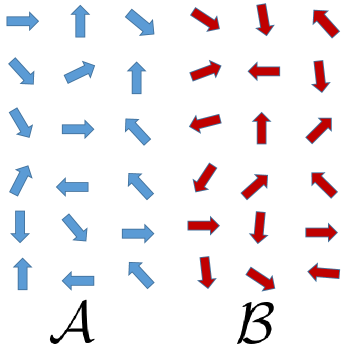
Figure 6: A typical configuration in calculating the second Rényi mutual information. There are two replicas (left and right) and each one is divided into two regions ${\cal A}$ and ${\cal B}$. Regions ${\cal A}$ of the two replicas are strongly correlated in the sense that an update of any spin in ${\cal A}$ is accepted only and only if the update affects the same spin in both replicas. On the other hand, the updates in regions ${\cal B}$ are independent in each replica.

The replica method enables us to compute the entanglement entropy and mutual information on the lattice PhysRevLett.106.135701 ; PhysRevLett.104.157201 . As we stressed before, unlike the entanglement entropy, which tells us about the amount of uncertainty in a system, mutual information, $I(X;Y)$, quantifies the amount of information shared between different parts of the system. Fortunately enough, one can calculate $I(X;Y)$ on the lattice using Monte Carlo methods. Here, we focus on the second Rényi Mutual information $I_{2}(X;Y)$ and consider the situation of a collection of spins located at the lattice sites. To this end, we bipartition a lattice ${\cal M}$ into two regions ${\cal A}$ and ${\cal B}$ and consider two replicas ${\cal M}_{1}$ and ${\cal M}_{2}$ such that ${\cal M}_{1}={\cal A}_{1}\cup{\cal B}_{1}$ and ${\cal M}_{2}={\cal A}_{2}\cup{\cal B}_{2}$. Now, we apply a boundary condition on the regions such that for a given configuration of spins on ${\cal A}_{1}$ and ${\cal A}_{2}$, which is taken to be the exact same configuration in both ${\cal A}_{1}$ and ${\cal A}_{2}$, we allow the spins in ${\cal B}_{1}$ and ${\cal B}_{2}$ to fluctuate independently, see Figure 6. This boundary condition amounts to tracing over the states of system ${\cal B}$ for a given state in ${\cal A}$. The partition function of the system is then given by the replicated partition function (43). According to $Z[{\cal A},2]$, Monte Carlo simulations will use the energy $E(x,y)+E(x,y^{\prime})$ to update the spin moves, which cannot be accepted unless it satisfies the above mentioned boundary condition. To be more specific, let us consider the Hamiltonian and partition function

$$E=-\sum_{\langle I,J\rangle}\bm{S}_{I}\cdot\bm{S}_{J}\,,\quad Z=\sum_{\{S_{I}\}}e^{-E/T}\,,$$ (52)

where the bracket indicates a sum over nearest neighbor pairs of spins. Then, the total energy of the replicated system is given by

$$E(x,y)+E(x,y^{\prime})=-2\sum_{\langle I_{A},I_{A}^{\prime}\rangle}\bm{S}_{I_{A}}\cdot\bm{S}_{I_{A}^{\prime}}-\sum_{\langle I_{B},I_{B}^{\prime}\rangle}\bm{S}_{I_{B}}\cdot\bm{S}_{I_{B}^{\prime}}-\sum_{\langle J_{B},J_{B}^{\prime}\rangle}\bm{S}_{J_{B}}\cdot\bm{S}_{J_{B}^{\prime}}\,.$$ (53)

We see that there is a factor of $2$ multiplying the first sum, which indicates that the effective temperature of region $\cal{A}$ is $T/2$. Hence, one needs to distinguish between three temperature ranges in the replicated system:

1. $0<T<T_{c}$, where $T_{c}$ is the critical temperature of the non-replicated system: both regions $\cal{A}$ and $\cal{B}$ are below criticality.

2. $T_{c}<T<2T_{c}$: region $\cal{B}$ is above criticality, while region ${\cal A}$ is below it.

3. $T>2T_{c}$: both regions $\cal{A}$ and $\cal{B}$ are above criticality.

Monte Carlo simulations don’t allow the direct computation of the partition function or entropy. In order to extract the entropy from simulations, one needs to integrate the energy estimator over a range of temperatures. The expectation value of energy is given by $\langle E\rangle=-\frac{\partial\log Z}{\partial\beta}$, and hence, using the definition (44) we find

$$S_{2}({\cal A};T)=\int_{T}^{\infty}\frac{dT^{\prime}}{T^{\prime 2}}\left[\langle E\rangle_{\cal A}(T^{\prime})-2\langle E\rangle_{0}(T^{\prime})\right]\,,$$ (54)

where $\langle E\rangle_{\cal A}$ and $\langle E\rangle_{0}$ are respectively the energy expectation values of the replicated and original (non-replicated) systems. Similarly, the Rényi Mutual information is given by the expression

$$I_{2}(X;Y;T)=\int_{T}^{\infty}\frac{dT^{\prime}}{T^{\prime 2}}\left[2\langle E\rangle_{\cal A}(T^{\prime})-2\langle E\rangle_{0}(T^{\prime})-\langle E\rangle_{{\cal A}\cup{\cal B}}(T^{\prime})\right]\,,$$ (55)

where $\langle E\rangle_{{\cal A}\cup{\cal B}}(T)$ is the energy of the replicated system as we shrink ${\cal B}$ to $\emptyset$, i.e., it is the energy of the original system at $T/2$.

In practice, we cutoff the integrals (54) and (55) at some $T_{max}\gg T$. Therefore, the extraction of entanglement entropy or mutual information in Monte Carlo method requires simulations over a large range of temperatures, an expensive and long process. Below, we show how one can partially circumvent this difficulty by making use of the T-dual description of the XY-spin lattice, which also eliminates unwanted vortices with lower winding number.

4.6 Mutual information from XY-spin models on the lattice and T-duality

As we showed above, the use of information theoretic techniques demands that we partition the system into two or more disjoint regions. This procedure introduces ambiguities in the lattice gauge theory calculations. Fortunately enough, we found that the gauge theory upon compactification is dual to XY-spin models. Such models do not suffer from ambiguities when studied on a lattice, and the extraction of entanglement entropy and mutual information from these systems is a more straightforward task.

The lattice version of the continuum XY-spin model (16) is given by

$$E=-\frac{K}{2\pi}\sum_{\langle I,J\rangle}\cos\left(\theta_{I}-\theta_{J}\right)-2G_{p}\sum_{I}\cos\left(p\theta_{I}\right)\,,\quad Z=\int_{0}^{2\pi}\prod_{i}d\theta_{i}e^{-E}$$ (56)

where we set the lattice spacing $a=1$. The equivalence between (56) and (16) is easily shown by expanding the first term in (56) to second order and taking $a\rightarrow 0$. As we showed in Section (3.2), there exists two equivalent XY-spin models for each of the theories we consider in this work. These models are the T-dual of eachother. This conclusion applies also to the lattice formulation, as we discuss momentarily. To be more specific we take QCD(adj) as an example. dYM and dYM(F) follow the same pattern.

In one of the descriptions the lattice partition function of QCD(adj) is given by (this is the lattice version of the continuum description (23))

$$E=-\frac{g^{2}}{16\pi^{2}}\sum_{\langle I,J\rangle}\cos\left(\theta_{I}-\theta_{J}\right)-2e^{-\frac{8\pi^{2}}{g^{2}}}\sum_{I}\cos\left(2\theta_{I}\right)\,,$$

$$Z[K=\frac{g^{2}}{8\pi T},G_{2}=\xi_{B},p=2;H_{2},w=2]=\int_{0}^{2\pi}\prod_{i}d\theta_{i}e^{-E/T}\,,$$ (57)

and we have set the size of the $\mathbb{S}_{L}^{1}$ circle equal to the lattice spacing, i.e., $L=a=1$. The description (57) has two pitfalls. First, one needs to strict the monodromies of $\{\theta_{I}\}$ to be even integers multiples of $2\pi$. This is necessary in order to eliminate the unit winding vortices from the spectrum of the theory (votices of unit windings are fundamental electric charges, which are absent in QCD(adj)). Second, as we found in Section (4.5), and according to Eq. (55), the extraction of mutual information from (57) entails performing extended Monte Carlo simulations.

The T-dual lattice description

In order to overcome these drawbacks, we switch to the T-dual description of (57). This is the lattice version of (24):

$$E=-\frac{4}{g^{2}}\sum_{\langle I,J\rangle}\cos\left(\theta_{I}-\theta_{J}\right)-2e^{-\frac{M_{W}}{T}}\sum_{I}\cos\left(4\theta_{I}\right)\,,$$

$$Z[K=\frac{8\pi T}{g^{2}},G_{4}=\xi_{W},p=4;H_{1},w=1]=\int_{0}^{2\pi}\prod_{i}d\theta_{i}e^{-TE}\,.$$ (58)

Now, we need not worry about suppressing lower-winding vertices in Monte Carlo simulations since magnetic bions (the magnetic excitations of QCD(adj)) in this description have unit windings. The same conclusion can be reached for dYM and dYM(F).

The coefficients that appear in the energy functional (58) (or the energy functional of dYM and dYM(F)) are not suitable for realistic Monte Carlo simulations given the extremely small values of the coupling constant and fugacities. Instead of (58), we replace it with the phenomenological model:

$$E=-\sum_{\langle I,J\rangle}\cos\left(\theta_{I}-\theta_{J}\right)-\tilde{y}\sum_{I}\cos\left(p\theta_{I}\right)\,,$$

$$Z[\tilde{y},p;H_{1},w=1]=\int_{0}^{2\pi}\prod_{i}d\theta_{i}e^{-TE}\,.$$ (59)

This model is capable of capturing the essential features of dYM, dYM(F), and QCD(adj) as follows:

1. $p=1$. This is dYM(F), where $p=1$ accounts for fundamental quarks and $T\tilde{y}$ is their fugacity. In principle, one should also add $\sum_{I}\cos(2\theta_{I})$ term to account for the W-bosons. However, the W-boson fugacity is exponentially small compared to that of the fundamental quarks, and it is more appropriate to neglect the W-bosons all together in the description. The unit-winding vortices, $w=1$, are magnetic monopoles.

2. $p=2$. This is dYM, where $p=2$ accounts for the W-bosons and $T\tilde{y}$ is their fugacity. Again, the unit-winding vortices are the magnetic monopoles.

3. $p=4$. This is QCD(adj), where $p=4$ denotes the W-bosons and $T\tilde{y}$ is their fugacity. The unit-winding vortices are the magnetic bions.

In all cases, exciting a unit-winding vortex costs a core energy, roughly, ${\cal O}(T)$ in lattice units, which is determined by the kinetic term in (59). Therefore, vortices are suppressed in the high temperature phase. On the other hand, as temperature increases, the fugacity of the electric excitations (fundamental quarks or W-bosons) increases, and hence, their core energies decrease. Thus, the electric excitations dominate the plasma at high temperatures. This is exactly the expected behavior in dYM, dYM(F), and QCD(adj), which is captured by the phenomenological model (59).

Although the phenomenological model (59) has ${\cal O}(1)$ fugacities, as opposed to the original system (58), which has an exponentially small fugacity owing to its semi-classical nature, it still captures the qualitative features of (58) since both models are expected to belong to the same universality class. For example, renormalization-group analysis of (58) (XY-pin model with $\mathbb{Z}_{4}$ symmetry-preserving perturbations and exponentially small fugacities) showed that it exhibits a continuous phase transition with a fugacity-dependent critical exponent Anber:2011gn . This behavior was also confirmed by Monte Carlo simulations of the phenomenological model (59), i.e., for large fugacities, see PhysRevB.69.174407 .

Now, we come to the point of extracting Rényi mutual information from (59). It is trivial to see that the expectation value of energy is $\langle E\rangle=-\frac{\partial Z}{\partial T}$, which replaces the traditional expression $\langle E\rangle=-\frac{\partial Z}{\partial\beta}$. This relation can be inverted to write the logarithm of the partition function as an integral over the energy estimator $\log Z=-\int_{0}^{T}dT^{\prime}\langle E\rangle(T^{\prime})$. Now, we make use of the definition (44) to find

$$I_{2}(X;Y;T)=\int_{0}^{T}dT^{\prime}\left[2\langle E\rangle_{\cal A}(T^{\prime})-2\langle E\rangle_{0}(T^{\prime})-\langle E\rangle_{{\cal A}\cup{\cal B}}(T^{\prime})\right]\,.$$ (60)

It is remarkable that the T-dual lattice model (59) provides a neat and cheap method to extract the mutual information compared to the original prescription (55), where one needs to suppress lower winding vortices.

When using the replica method (we use only two replicas in this work) to compute $I_{2}(X;Y;T)$, one needs to distinguish between three temperature regimes in (59) (as usual we divide our lattice into two regions ${\cal A}$ and ${\cal B}$ such that the spins of regions ${\cal A}$ of the two replicas are updated simultaneously). Since the temperature $T$ multiplies the energy functional in (59), region $A$ will effectively be at temperatures twice that of the original system. The three temperature regimes are:

1. $0<T<T_{c}/2$, where $T_{c}$ is the critical temperature of the non-replicated system: both regions $\cal{A}$ and $\cal{B}$ are below criticality.

2. $T_{c}/2<T<T_{c}$: region $\cal{A}$ is above criticality, while region ${\cal B}$ is below it.

3. $T>T_{c}$: both regions $\cal{A}$ and $\cal{B}$ are above criticality.

In the next section we perform numerical simulations of (59) and extract lessons from $I_{2}(X;Y;T)$ about the deconfinement phase transition/crossover.

5 Monte Carlo simulations

This section is devoted to the numerical simulations of (59). In particular, we show that mutual information can be used as a probe to detect phase transitions in our theories.

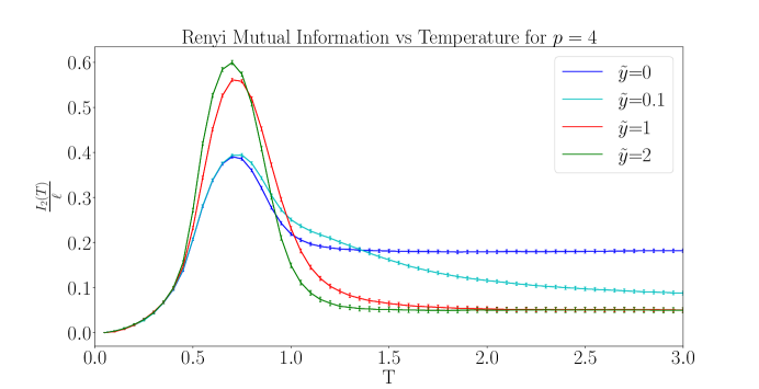
Figure 7: Mutual information of (59) for $p=4$ and various values of $\tilde{y}$. We use lattice size $N=16$.

We use a single-flip Metropolis algorithm and divide our periodic lattice of size $N\times N$ into two regions ${\cal A}={\cal B}$, such that each region is $N\times N/2$ cylinder embedded in $N\times N$ torus. We start by studying Rényi mutual information (RMI) of (59) with $p=4$, QCD(adj), and various values of $\tilde{y}$. The results are shown in Figure 7, where we plot $I_{2}(X;Y;T)/\ell$ against the temperature and $\ell=2N$ is the length of the boundary between regions ${\cal A}$ and ${\cal B}$. First, we see that all RMI curves coincide at small $T$, irrespective of the value of $\tilde{y}$. This is consistent with the fact that the electric excitations are confined at low temperatures, their fugacities are irrelevant, and the system is dominated by a plasma of magnetic charges. The correlation length in a plasma is extremely small and the different parts of the system are uncorrelated. This is reflected in the fact that RMI is vanishingly small at low temperature. As we dial up $T$, the density of the magnetic charges decreases, the correlation length increases, and information can be communicated across larger distances. This can be seen as a spike in RMI, with a magnitude that depends on the value of $\tilde{y}$. At high enough temperatures (above the critical temperature $T_{c}$; we will determine $T_{c}$ below) RMI asymptotes to a constant value, which decreases with increasing $\tilde{y}$. In order to understand the significance of this behavior, we compare $\tilde{y}=0$ with $\tilde{y}=0.1,1.0,2.0$. The former case corresponds to eliminating W-bosons from our theory. In this case the system exhibits a BKT phase transition, from a massive to massless phase, as we dial up the temperature. This is in contradistinction with the case $\tilde{y}>0$: dialing up the temperature will cause the system to transit from a massive (magnetic) phase to another massive (electric) phase. Obviously, a massless phase can communicate information more effectively than a massive one, and thus, at high enough temperatures RMI attains larger values. Also, the bigger the value of $\tilde{y}$, the higher the density of W-bosons in the electric disordered phase and the lower the value of the asymptotic RMI.

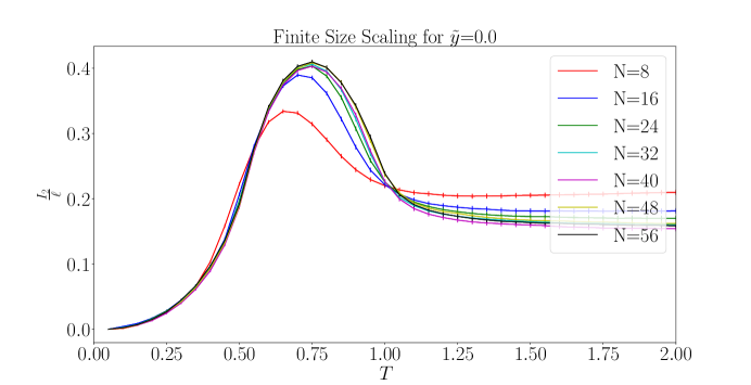
Figure 8: Finite size scaling for RMI of (59) with $\tilde{y}=0$. The curves cross at $T\cong 0.5$ and $T\cong 1$, which are the values of $T_{c}/2$ and $T_{c}$, respectively.

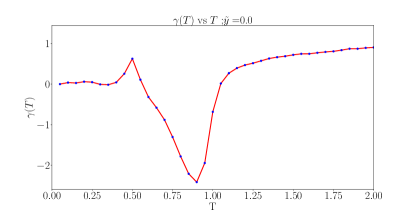
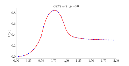
Figure 9: The fitting of $I(X;Y,T)$ to $C(T)N+\gamma(T)$ for $\tilde{y}=0$. The data is obtained from fitting lattice sizes $N=8$ to $N=56$.

Next, we further examine the case $\tilde{y}=0$ for different lattice sizes. The results are shown in Figure 8 for $N=8$ to $N=56$. We see that all the curves collapse onto a single curve for large values of $N$. This behavior is consistent with the assertion that Rényi mutual information follows the area law scaling $I(X;Y;T)={\cal C}(T)\ell+\gamma(T)$, where ${\cal C}(T)$ and $\gamma(T)$ are temperature-dependent coefficients. This behavior holds even at criticality and can be used to extract the critical temperature, as we will see momentarily. As we discussed at the end of Section 4.6, the replicated system exhibits two critical temperatures at $T_{c}/2$ and $T_{c}$. The system becomes scale invariant at these two points. Therefore, we expect $I(X;Y,T)/\ell$ to be a constant for all lattice sizes, and hence, $\gamma(T)$ is expected to cross zero near $T_{c}/2$ and $T_{c}$. This behavior is easily seen in Figure 9, where we fit ${\cal C}(T)$ and $\gamma(T)$ using RMI data from $N=16$ to $N=56$. We also see that ${\cal C}(T)$ attains the asymptotic shape of Figure 8. This explains the crossing of RMI curves and then their fan out at $T_{c}/2$ and $T_{c}$. Thus, the finite size scaling of RMI can be used as a probe to search for phase transitions PhysRevB.87.195134 . Interestingly enough, the model given by (59) and $\tilde{y}=0$ (the T-dual XY spin model with no $\mathbb{Z}_{p}$ symmetry-preserving perturbation) does not have an order parameter that can be used to study the BKT phase transition. Instead, one traditionally uses the spin stiffness to accurately estimate the critical temperature Nelson:1977zz ; 0305-4470-38-26-003 . RMI provides an alternative probe to accurately study phase transitions in this mode, see PhysRevB.87.195134 for more details. We elaborate more on this point below.

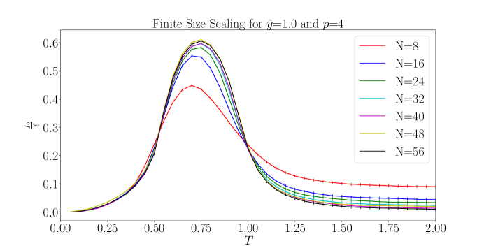
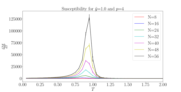
Figure 10: Top panel: the finite size scaling for RMI of (59) with $p=4$ and $\tilde{y}=1$. This case corresponds to QCD(adj). The curves cross at $T\cong 0.5$ and $T\cong 1$, which are the values of $T_{c}/2$ and $T_{c}$, respectively. Bottom panel: the magnetic susceptibility of the system. The susceptibility peaks at $T\cong 1$, in agreement with RMI.

QCD(adj)

Now, we move to the finite size scaling of QCD(adj). RMI for different lattice sizes of this theory is depicted in the top panel of Figure 10, where we used $\tilde{y}=1$ for our study. The curves cross at $T_{c}/2$ and $T_{c}$ with $T_{c}\cong 1$. We also calculate the magnetic susceptibility of the system, which is given by

$$\chi_{M}=\frac{d|M|}{dT}\,,\quad M=\sum_{j}^{N^{2}}e^{i\theta_{j}}\,.$$ (61)

QCD(adj) is invariant under $\mathbb{Z}_{4}$ symmetry: $\theta_{j}\rightarrow\theta_{j}+\frac{2\pi}{4}$, while $M\rightarrow iM$ under the same symmetry. Therefore, $|M|$ and $\chi_{M}$ are good order parameters of the system. We plot $\chi_{M}$ in the bottom panel of Figure 10. We see that the susceptibility peaks at $T_{c}\cong 1$, in agreement with RMI calculations. Comparing Figures 8 and 10, we see that the transition temperature is independent of $\tilde{y}$. This is in disagreement with the calculations of the transition temperatures in Section (3.3). One can see from the discussion of the dual Sine-Gordon model and Figures (4) and (5) that $T_{c\,,y=0}=2T_{c\,,QCD(adj)}$. This disagreement, however, should not come as a surprise since unlike the dual Sine-Gordon model, where both electric and magnetic fugacities are explicit parameters, the magnetic core energy of (59) is not an under-control explicit parameter. In fact, the transition temperature of the XY-spin models have only a mild dependence on the electric fugacity, as was also found in previous studies PhysRevB.69.174407 .

We also fit $I(X;Y;T)$ to the form $C(T)N+\gamma(T)$. The results are shown in Figure 11. It is clear that $\gamma(T)$ changes signs at $T_{c}/2$ and $T_{c}$, while $C(T)$ attains the asymptotic shape of RMI in Figure 10. This explains the crossing of RMI curves at these two points, similar to the case $\tilde{y}=0$.

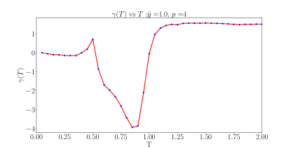
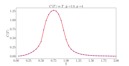
Figure 11: The fitting of $I(X;Y,T)$ to $C(T)N+\gamma(T)$ for $p=4$ and $\tilde{y}=1$. The data is obtained from fitting lattice sizes $N=8$ to $N=56$.

dYM and dYM(F)

We repeat the above analysis for dYM, $p=2$, and dYM(F), $p=1$. dYM is invariant under $\mathbb{Z}_{2}$ symmetry: $\theta_{j}\rightarrow\theta_{j}+\frac{2\pi}{2}$ and $|M|$ and $\chi_{M}$ are good order parameters of the system. RMI and magnetic susceptibility of dYM with $\tilde{y}=1$ are shown in Figure 12 . Again, the peak of the susceptibility coincides with the second crossing of RMI curves indicating that the latter can probe phase transitions in this system.

On the other hand, dYM(F) does not entertain any global symmetry. RMI of dYM(F) with $\tilde{y}=1$ is shown in Figure 13. Unlike all previous cases, RMI of different lattice sizes do not show any features of a phase transition. Also, the amplitude of RMI for $p=1$ is suppressed compared to that of $p>1$. We anticipate that this behavior is tied to the absence of global symmetries in this theory and that the theory experiences a smooth crossover from one phase to the other. We further comment on this behavior in the Discussion Section.

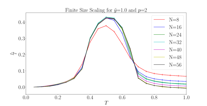
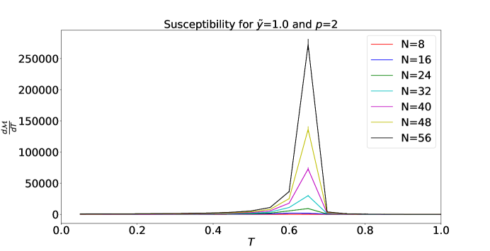
Figure 12: Top panel: the finite size scaling for RMI of (59) with $p=2$ and $\tilde{y}=1$. This case corresponds to dYM. The curves cross at $T\cong 0.32$ and $T\cong 0.65$, which are the values of $T_{c}/2$ and $T_{c}$, respectively. Bottom panel: the magnetic susceptibility of the system. The susceptibility peaks at $T\cong 0.65$, in agreement with RMI.

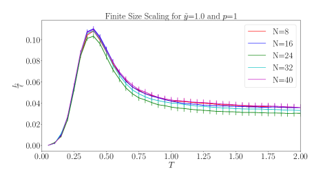
Figure 13: RMI for $p=1$ and $\tilde{y}=1$. This case corresponds to dYM(F). Unlike the previous cases, RMI of different sizes does not show any features of a phase transition.

6 Discussion and future directions

In this paper we studied the deconfinement transition in Yang-Mills theory on $\mathbb{R}^{2}\times\mathbb{T}^{2}$ by means of information-theoretic techniques in the continuum and on the lattice. The entanglement entropy calculations were achieved in the continuum via mapping the theory to a dual Sine-Gordon model. We found that this quantity attains a maximum value in dYM, dYM(F), and QCD(adj) at the transition/crossover point. The maximum is attributed to the interchange of the role of both the magnetic and electric charges. We also calculated Rényi mutual information (RMI) using a lattice version of the XY-spin model with ${\mathbb{Z}_{p}}$ symmetry-preserving perturbations. Unlike the entanglement entropy, which only captures the amount of uncertainty about the system, mutual information gives a quantitative measure of the information shared between different parts of the system. Our RMI study is free from ambiguities that usually plague lattice gauge theories due to the non factorizability of the gauge invariant Hilbert space. We found that RMI follows the area law scaling, with subleading corrections, and their finite size scaling can be used to search for phase transitions in our theories. In particular, there is a clear crossing of RMI curves at the transition temperature in both dYM and QCD(adj), while the addition of fundamental matter washes out the crossing and dilute the information that can be shared between the system parts. As a byproduct, we also found a new method to efficiently extract RMI without the need to suppress low-winding vortices. This is done by using a T-dual description of the XY-spin model. The web of dualities in our work is tied up to the fact that Yang-Mills theory on $\mathbb{R}^{2}\times\mathbb{T}^{2}$ (with deformations or adjoint fermions) can be mapped to a dual Coulomb gas, which faithfully captures all the effective degrees of freedom near the deconfinement transition.

dYM has a $\mathbb{Z}_{2}^{C}$ center symmetry that breaks in the deconfined phase. On the other hand, QCD(adj) enjoys $\mathbb{Z}_{2}^{C}$ center and $\mathbb{Z}_{2}^{d\chi}$ discrete chiral symmetries. $\mathbb{Z}_{2}^{d\chi}$ is broken in the low temperature phase and gets restored in the deconfined phase. The renormalization group calculations conducted in Anber:2011gn and our simulations indicate that the breaking of $\mathbb{Z}_{2}^{C}$ and restoration of $\mathbb{Z}_{2}^{d\chi}$ occurs at exactly the same critical temperature. In fact there is a constraint on the order of the occurrence of deconfinement and discrete chiral symmetry restoration in gauge theories: $T_{\scriptsize\mbox{decon}}\leq T_{\scriptsize\mbox{chiral}}$. This inequality is implied from the $\mathbb{Z}_{2}^{d\chi}$-$\left[\mathbb{Z}_{2}^{C}\right]^{2}$ mixed ’t Hooft anomaly, as was shown in Shimizu:2017asf ; Komargodski:2017smk . Deconfinemnet in QCD(adj) on $\mathbb{R}^{2}\times\mathbb{T}^{2}$ saturates this inequality.

Adding fundamental matter to dYM breaks the center explicitly. In this case RMI does not reveal any feature near the crossover, which is otherwise captured by the entanglement entropy of the dual Sine-Gordon model. We also found that RMI of pure XY-spin model (no $\mathbb{Z}_{p}$ symmetry-preserving perturbations) captures the transition, while entanglement entropy doesn’t show any specific feature near the transition.

Before concluding our work, it is amusing to reflect on the role RMI could have played in 2-D physics had we learned about it half a century ago. First, let us note that Mermin-Wagner theorem was published in 1966, 6 years before the discovery of the BKT phase transition. This theorem forbids continuous phase transitions in 2D, and hence, BKT phase transition in XY model came as a surprise to the physics community in 1973. Had people calculated RMI (which was not known by that time, at least among the physics community) of XY model with different $Z_{p}$ symmetry-preserving perturbations before 1973, they would have revealed that pure XY model (with no perturbations) is in tension with Mermin-Wagner theorem. For any $p\neq 1$ there is a discrete symmetry and symmetry breaking can happen (Mermin-Wagner theorem is no-go only for continuous symmetries). The crossing of RMI curves at a certain temperature signals the breaking of the $\mathbb{Z}_{p}$ symmetry. When $p=1$, on the other hand, the system doesn’t enjoy any kind of symmetry, and hence, no crossing of RMI should be expected. This is exactly what we see in our simulations. The striking thing, however, is when we set the perturbations to zero. Although there is a $U(1)$ symmetry in one of the phases, Mermin-Wagner theorem forbids genuine symmetry breaking. RMI curves, on the other hand, have a clear crossing indicating that there is a nontrivial transition in the system. This is what Berezinskii, Kosterlitz, and Thouless discovered in 1973.

On the gauge theory side, we know on symmetry grounds that the presence of fundamental quarks eliminates the possibility of using the Polyakov’s loop as a probe to detect phase transformations. One, however, could argue that near the transition (or crossover) the confined pairs of fundamentals and W-bosons would simply liberate making no striking difference between the presence and absence of fundamentals in the picture. Contrary to this expectation, our simulations indicate that the presence of fundamentals makes a dramatic difference, at least from information theory point of view. This points to a tantalizing link between the absence/presence of symmetries and information stored in a system.

Future directions

1. The special case of QCD(adj) on $\mathbb{R}^{3}\times\mathbb{T}^{2}$ with a single fermionic flavor is ${\cal N}=1$ supersymmetric glue dynamics. Deconfinement in this theory was extensively discussed in Anber:2013doa with conclusions similar to that of QCD(adj). The computation of RMI in this theory near the critical temperature will be discussed in a future work. We expect, however, that supersymmetry will not greatly affect the conclusions of our present work.

2. In Anber:2012ig an $SU(3)$ QCD(adj) theory on $\mathbb{R}^{2}\times\mathbb{T}^{2}$ was studied via the dual Coulomb gas/ XY-spin model duality, and it was concluded that the deconfinement transition is first order. It will be interesting to examine whether RMI can have a nontrivial behavior at the transition point in this system.

3. Our work has also applications beyond gauge theory. The study of RMI to identify classical transitions was first applied to the Ising and XY-models in PhysRevB.87.195134 and later extended to other systems like the classical toric code model PhysRevB.92.125144 . In fact, XY-spin models with perturbations are universal models that have a wide range of applications from the roughing transitions to the 2-D solid melting, see Wen:2004ym . The calculations of RMI may help in identifying interesting features near the phase transition in these systems.

4. Another interesting quantity that can be readily measured in XY-spin systems is the topological entanglement entropy, the constant term in $S=C\ell+\gamma_{\scriptsize\mbox{top}}$. This quantity is nonzero in systems that exhibit topological order, and hence, can be descried by topological field theories (TFT) deep in the IR. The existence of discrete ’t Hooft anomalies in QCD(adj) suggests that this theory may admit a TFT that saturates the anomaly. The topological entanglement entropy can be calculated using either Levin and Wen PhysRevLett.96.110405 or Kitaev and Preskil PhysRevLett.96.110404 schemes. Whether $\gamma_{\scriptsize\mbox{top}}$ is non-vanishing in QCD(adj) is left for a future investigation.

5. Information about the CFT universality class can be extracted from RMI at the critical temperature. This can be done by computing RMI for different partitions of a given lattice size and trying to fit the next to leading term of RMI (the leading term is being the area) with general known behavior of CFT at finite interval. This will elucidate the link between the entanglement entropy of the dual Sine-Gordon model (which we examined in this work via CFT with deformations) and RMI of the XY models.

6. Finally, it will be interesting to compute RMI of the full scale 4-D theory on the lattice and examine whether this quantity has a similar behavior, near the transition, to the one found in this work.

- (1) N. Laflorencie, Quantum entanglement in condensed matter systems, Phys. Rept. 646 (2016) 1–59, [arXiv:1512.03388].
- (2) B. Zeng, X. Chen, D.-L. Zhou, and X.-G. Wen, Quantum Information Meets Quantum Matter – From Quantum Entanglement to Topological Phase in Many-Body Systems, ArXiv e-prints (Aug., 2015) [arXiv:1508.02595].
- (3) D. N. Kabat, Black hole entropy and entropy of entanglement, Nucl. Phys. B453 (1995) 281–299, [hep-th/9503016].
- (4) P. V. Buividovich and M. I. Polikarpov, Numerical study of entanglement entropy in SU(2) lattice gauge theory, Nucl. Phys. B802 (2008) 458–474, [arXiv:0802.4247].
- (5) A. R. Zhitnitsky, Entropy, Contact Interaction with Horizon and Dark Energy, Phys. Rev. D84 (2011) 124008, [arXiv:1105.6088].
- (6) S. N. Solodukhin, Remarks on effective action and entanglement entropy of Maxwell field in generic gauge, JHEP 12 (2012) 036, [arXiv:1209.2677].
- (7) W. Donnelly and A. C. Wall, Do gauge fields really contribute negatively to black hole entropy?, Phys. Rev. D86 (2012) 064042, [arXiv:1206.5831].
- (8) C. Eling, Y. Oz, and S. Theisen, Entanglement and Thermal Entropy of Gauge Fields, JHEP 11 (2013) 019, [arXiv:1308.4964].
- (9) C. A. Agon, M. Headrick, D. L. Jafferis, and S. Kasko, Disk entanglement entropy for a Maxwell field, Phys. Rev. D89 (2014), no. 2 025018, [arXiv:1310.4886].
- (10) K.-W. Huang, Central Charge and Entangled Gauge Fields, Phys. Rev. D92 (2015), no. 2 025010, [arXiv:1412.2730].
- (11) W. Donnelly, B. Michel, and A. Wall, Electromagnetic Duality and Entanglement Anomalies, Phys. Rev. D96 (2017), no. 4 045008, [arXiv:1611.05920].
- (12) H. Casini, M. Huerta, and J. A. Rosabal, Remarks on entanglement entropy for gauge fields, Phys. Rev. D89 (2014), no. 8 085012, [arXiv:1312.1183].
- (13) D. Radicevic, Notes on Entanglement in Abelian Gauge Theories, arXiv:1404.1391.
- (14) S. Ghosh, R. M. Soni, and S. P. Trivedi, On The Entanglement Entropy For Gauge Theories, JHEP 09 (2015) 069, [arXiv:1501.02593].
- (15) S. Aoki, T. Iritani, M. Nozaki, T. Numasawa, N. Shiba, and H. Tasaki, On the definition of entanglement entropy in lattice gauge theories, JHEP 06 (2015) 187, [arXiv:1502.04267].
- (16) K. Van Acoleyen, N. Bultinck, J. Haegeman, M. Marien, V. B. Scholz, and F. Verstraete, The entanglement of distillation for gauge theories, Phys. Rev. Lett. 117 (2016), no. 13 131602, [arXiv:1511.04369].
- (17) S. Ryu and T. Takayanagi, Holographic derivation of entanglement entropy from AdS/CFT, Phys. Rev. Lett. 96 (2006) 181602, [hep-th/0603001].
- (18) T. Nishioka and T. Takayanagi, AdS Bubbles, Entropy and Closed String Tachyons, JHEP 01 (2007) 090, [hep-th/0611035].
- (19) I. R. Klebanov, D. Kutasov, and A. Murugan, Entanglement as a probe of confinement, Nucl. Phys. B796 (2008) 274–293, [arXiv:0709.2140].
- (20) M. Fujita, T. Nishioka, and T. Takayanagi, Geometric Entropy and Hagedorn/Deconfinement Transition, JHEP 09 (2008) 016, [arXiv:0806.3118].
- (21) A. Velytsky, Entanglement entropy in d+1 SU(N) gauge theory, Phys. Rev. D77 (2008) 085021, [arXiv:0801.4111].
- (22) M. Unsal, Magnetic bion condensation: A New mechanism of confinement and mass gap in four dimensions, Phys. Rev. D80 (2009) 065001, [arXiv:0709.3269].
- (23) E. Poppitz, T. Schafer, and M. Unsal, Continuity, Deconfinement, and (Super) Yang-Mills Theory, JHEP 10 (2012) 115, [arXiv:1205.0290].
- (24) E. Poppitz, T. Schafer, and M. Unsal, Universal mechanism of (semi-classical) deconfinement and theta-dependence for all simple groups, JHEP 03 (2013) 087, [arXiv:1212.1238].
- (25) M. M. Anber, E. Poppitz, and B. Teeple, Deconfinement and continuity between thermal and (super) Yang-Mills theory for all gauge groups, JHEP 09 (2014) 040, [arXiv:1406.1199].
- (26) M. M. Anber and V. Pellizzani, Representation dependence of k -strings in pure Yang-Mills theory via supersymmetry, Phys. Rev. D96 (2017), no. 11 114015, [arXiv:1710.06509].
- (27) M. M. Anber, E. Poppitz, and M. Unsal, 2d affine XY-spin model/4d gauge theory duality and deconfinement, JHEP 04 (2012) 040, [arXiv:1112.6389].
- (28) L. P. Kadanoff, Lattice Coulomb Gas Representations of Two-Dimensional Problems, J. Phys. A11 (1978) 1399–1417.
- (29) I. I. Kogan and A. Kovner, Monopoles, vortices and strings: Confinement and deconfinement in (2+1)-dimensions at weak coupling, hep-th/0205026.
- (30) J. Liao and E. Shuryak, Strongly coupled plasma with electric and magnetic charges, Phys. Rev. C75 (2007) 054907, [hep-ph/0611131].
- (31) M. M. Anber, The abelian confinement mechanism revisited: new aspects of the Georgi-Glashow model, Annals Phys. 341 (2014) 21–55, [arXiv:1308.0027].
- (32) B. Svetitsky and L. G. Yaffe, Critical Behavior at Finite Temperature Confinement Transitions, Nucl. Phys. B210 (1982) 423–447.
- (33) M. Unsal and L. G. Yaffe, Center-stabilized Yang-Mills theory: Confinement and large N volume independence, Phys. Rev. D78 (2008) 065035, [arXiv:0803.0344].
- (34) D. J. Gross, R. D. Pisarski, and L. G. Yaffe, QCD and Instantons at Finite Temperature, Rev. Mod. Phys. 53 (1981) 43.
- (35) N. M. Davies, T. J. Hollowood, and V. V. Khoze, Monopoles, affine algebras and the gluino condensate, J. Math. Phys. 44 (2003) 3640–3656, [hep-th/0006011].
- (36) M. M. Anber and E. Poppitz, New nonperturbative scales and glueballs in confining supersymmetric gauge theories, arXiv:1711.00027.
- (37) M. M. Anber, S. Collier, E. Poppitz, S. Strimas-Mackey, and B. Teeple, Deconfinement in super Yang-Mills theory on via dual-Coulomb gas and ”affine” XY-model, JHEP 11 (2013) 142, [arXiv:1310.3522].
- (38) G. V. Dunne, Y. Tanizaki, and M. Ünsal, Quantum Distillation of Hilbert Spaces, Semi-classics and Anomaly Matching, arXiv:1803.02430.
- (39) A. Cherman and M. Unsal, Critical behavior of gauge theories and Coulomb gases in three and four dimensions, arXiv:1711.10567.
- (40) A. Cherman, S. Sen, M. Unsal, M. L. Wagman, and L. G. Yaffe, Order parameters and color-flavor center symmetry in QCD, Phys. Rev. Lett. 119 (2017), no. 22 222001, [arXiv:1706.05385].
- (41) Y. Tanizaki, T. Misumi, and N. Sakai, Circle compactification and ’t Hooft anomaly, JHEP 12 (2017) 056, [arXiv:1710.08923].
- (42) E. Poppitz and M. E. Shalchian T., String tensions in deformed Yang-Mills theory, JHEP 01 (2018) 029, [arXiv:1708.08821].
- (43) K. Aitken, A. Cherman, E. Poppitz, and L. G. Yaffe, QCD on a small circle, Phys. Rev. D96 (2017), no. 9 096022, [arXiv:1707.08971].
- (44) M. M. Anber and A. R. Zhitnitsky, Oblique Confinement at in weakly coupled gauge theories with deformations, Phys. Rev. D96 (2017), no. 7 074022, [arXiv:1708.07520].
- (45) A. Cherman and E. Poppitz, Emergent dimensions and branes from large- confinement, Phys. Rev. D94 (2016), no. 12 125008, [arXiv:1606.01902].
- (46) M. M. Anber and E. Poppitz, On the global structure of deformed Yang-Mills theory and QCD(adj) on , JHEP 10 (2015) 051, [arXiv:1508.00910].
- (47) M. M. Anber and E. Poppitz, Microscopic Structure of Magnetic Bions, JHEP 06 (2011) 136, [arXiv:1105.0940].
- (48) T. C. Kraan and P. van Baal, Monopole constituents inside SU(n) calorons, Phys. Lett. B435 (1998) 389–395, [hep-th/9806034].
- (49) K.-M. Lee and P. Yi, Monopoles and instantons on partially compactified D-branes, Phys. Rev. D56 (1997) 3711–3717, [hep-th/9702107].
- (50) A. M. Polyakov, Quark Confinement and Topology of Gauge Groups, Nucl. Phys. B120 (1977) 429–458.
- (51) R. Jackiw and C. Rebbi, Solitons with Fermion Number 1/2, Phys. Rev. D13 (1976) 3398–3409.
- (52) C. Csaki, Y. Shirman, J. Terning, and M. Waterbury, Twisted Sisters: KK Monopoles and their Zero Modes, arXiv:1708.03330.
- (53) C. Callias, Index Theorems on Open Spaces, Commun. Math. Phys. 62 (1978) 213–234.
- (54) T. M. W. Nye and M. A. Singer, An L**2 index theorem for Dirac operators on S**1 x R**3, Submitted to: J. Funct. Anal. (2000) [math/0009144].
- (55) E. Poppitz and M. Unsal, Index theorem for topological excitations on R**3 x S**1 and Chern-Simons theory, JHEP 03 (2009) 027, [arXiv:0812.2085].
- (56) B. Teeple, Deconfinement on for all gauge groups and duality to double Coulomb Gas, JHEP 04 (2016) 109, [arXiv:1506.02110].
- (57) G. V. Dunne, I. I. Kogan, A. Kovner, and B. Tekin, Deconfining phase transition in (2+1)-dimensions: The Georgi-Glashow model, JHEP 01 (2001) 032, [hep-th/0010201].
- (58) J. V. Jose, L. P. Kadanoff, S. Kirkpatrick, and D. R. Nelson, Renormalization, vortices, and symmetry breaking perturbations on the two-dimensional planar model, Phys. Rev. B16 (1977) 1217–1241.
- (59) J. Zinn-Justin, Quantum field theory and critical phenomena, Int. Ser. Monogr. Phys. 113 (2002) 1–1054.
- (60) X. G. Wen, Quantum field theory of many-body systems: From the origin of sound to an origin of light and electrons. 2004.
- (61) Y. V. Kovchegov and D. T. Son, Critical temperature of the deconfining phase transition in (2+1)-d Georgi-Glashow model, JHEP 01 (2003) 050, [hep-th/0212230].
- (62) D. Boyanovsky, Field Theoretical Renormalization and Fixed Point Structure of a Generalized Coulomb Gas, J. Phys. A22 (1989) 2601–2614.
- (63) D. Boyanovsky and R. Holman, Critical behavior and duality in extended Sine-Gordon theories, Nucl. Phys. B358 (1991) 619–653.
- (64) J. B. Zuber and C. Itzykson, Quantum Field Theory and the Two-Dimensional Ising Model, Phys. Rev. D15 (1977) 2875.
- (65) P. Lecheminant, A. O. Gogolin, and A. A. Nersesyan, Criticality in selfdual sine-Gordon models, Nucl. Phys. B639 (2002) 502–523, [cond-mat/0203294].
- (66) M. A. Nielsen and I. L. Chuang, Quantum Computation and Quantum Information: 10th Anniversary Edition. Cambridge University Press, New York, NY, USA, 10th ed., 2011.
- (67) J. D. Bekenstein, Black holes and entropy, Phys. Rev. D7 (1973) 2333–2346.
- (68) J. M. Bardeen, B. Carter, and S. W. Hawking, The Four laws of black hole mechanics, Commun. Math. Phys. 31 (1973) 161–170.
- (69) G. ’t Hooft, On the Quantum Structure of a Black Hole, Nucl. Phys. B256 (1985) 727–745.
- (70) G. Vidal, J. I. Latorre, E. Rico, and A. Kitaev, Entanglement in quantum critical phenomena, Phys. Rev. Lett. 90 (Jun, 2003) 227902.
- (71) M. M. Wolf, F. Verstraete, M. B. Hastings, and J. I. Cirac, Area laws in quantum systems: Mutual information and correlations, Phys. Rev. Lett. 100 (Feb, 2008) 070502.
- (72) M. A. Metlitski and T. Grover, Entanglement Entropy of Systems with Spontaneously Broken Continuous Symmetry, arXiv:1112.5166.
- (73) M. Cramer, J. Eisert, M. B. Plenio, and J. Dreißig, Entanglement-area law for general bosonic harmonic lattice systems, Phys. Rev. A 73 (Jan, 2006) 012309.
- (74) J. Iaconis, S. Inglis, A. B. Kallin, and R. G. Melko, Detecting classical phase transitions with renyi mutual information, Phys. Rev. B 87 (May, 2013) 195134.
- (75) C. G. Callan, Jr. and F. Wilczek, On geometric entropy, Phys. Lett. B333 (1994) 55–61, [hep-th/9401072].
- (76) J.-M. Stéphan, S. Inglis, P. Fendley, and R. G. Melko, Geometric mutual information at classical critical points, Phys. Rev. Lett. 112 (Mar, 2014) 127204.
- (77) P. Banerjee, A. Bhatta, and B. Sathiapalan, Sine-Gordon Theory : Entanglement entropy and holography, Phys. Rev. D96 (2017), no. 12 126014, [arXiv:1610.04233].
- (78) P. Calabrese and J. L. Cardy, Entanglement entropy and quantum field theory, J. Stat. Mech. 0406 (2004) P06002, [hep-th/0405152].
- (79) V. L. Berezinsky, Destruction of long range order in one-dimensional and two-dimensional systems having a continuous symmetry group. 1. Classical systems, Sov. Phys. JETP 32 (1971) 493–500. [Zh. Eksp. Teor. Fiz.59,907(1971)].
- (80) J. M. Kosterlitz and D. J. Thouless, Ordering, metastability and phase transitions in two-dimensional systems, J. Phys. C6 (1973) 1181–1203.
- (81) R. R. P. Singh, M. B. Hastings, A. B. Kallin, and R. G. Melko, Finite-temperature critical behavior of mutual information, Phys. Rev. Lett. 106 (Mar, 2011) 135701.
- (82) M. B. Hastings, I. González, A. B. Kallin, and R. G. Melko, Measuring renyi entanglement entropy in quantum monte carlo simulations, Phys. Rev. Lett. 104 (Apr, 2010) 157201.
- (83) E. Rastelli, S. Regina, and A. Tassi, Monte carlo simulation of a planar rotator model with symmetry-breaking fields, Phys. Rev. B 69 (May, 2004) 174407.
- (84) D. R. Nelson and J. M. Kosterlitz, Universal Jump in the Superfluid Density of Two-Dimensional Superfluids, Phys. Rev. Lett. 39 (1977) 1201–1205.
- (85) M. Hasenbusch, The two-dimensional xy model at the transition temperature: a high-precision monte carlo study, Journal of Physics A: Mathematical and General 38 (2005), no. 26 5869.
- (86) H. Shimizu and K. Yonekura, Anomaly constraints on deconfinement and chiral phase transition, arXiv:1706.06104.
- (87) Z. Komargodski, T. Sulejmanpasic, and M. Ünsal, Walls, anomalies, and deconfinement in quantum antiferromagnets, Phys. Rev. B97 (2018), no. 5 054418, [arXiv:1706.05731].
- (88) M. M. Anber, S. Collier, and E. Poppitz, The QCD(adj) deconfinement transition via the gauge theory/’affine’ XY-model duality, JHEP 01 (2013) 126, [arXiv:1211.2824].
- (89) J. Helmes, J.-M. Stéphan, and S. Trebst, Rényi entropy perspective on topological order in classical toric code models, Phys. Rev. B 92 (Sep, 2015) 125144.
- (90) M. Levin and X.-G. Wen, Detecting topological order in a ground state wave function, Phys. Rev. Lett. 96 (Mar, 2006) 110405.
- (91) A. Kitaev and J. Preskill, Topological entanglement entropy, Phys. Rev. Lett. 96 (Mar, 2006) 110404.