Convergence Analysis of Shift-Inverse Method with Richardson Iteration For Eigenvalue Problem

Abstract

In this paper, we consider the shift-inverse method with Richardson iteration step for the eigenvalue problems. It will be shown that the convergence speed depends heavily on the eigenvalue gap between the desired eigenvalue and undesired ones.

Keywords. Eigenvalue problem, shift-inverse method, Richardson iteration AMS subject classifications. 65N30, 65N25, 65L15, 65B99.

1 Introduction

This paper is to discuss the convergence behavior of the Richardson iteration step in the shift-inverse (or Rayleigh quotient) method for the eigenvalue problem. It is well known that the shift-inverse method has a superlinear convergence order if we have good enough initial guesses (cf. [1, 3, 2]). But in the shift-inverse method, we need to solve the almost singular linear system which is not so easy work. Thus it is necessary to consider the effectiveness of the iteration steps for the almost singular systems. The first aim of this paper is to discuss the Richardson iteration step applied to the linear equations deduced from the shift-inverse method for the eigenvalue problem. The common idea is that it should be difficult to solve the linear equations since they are almost singular when the shift close to a singular. We will show here that the common iteration method can also work very well for these linear equations since the final aim is to find the eigenvectors rather than solving the deduced linear equations. The most important property is that the iteration step can reduce the relative scale of the undesired eigenvectors according to the desired eigenvectors. After normalization, the errors in the undersired eigenvectors will become smaller and smaller.

The rest of this paper is organized as follows. In the next section, we introduce the shift-inverse method and the Richardson iteration for the shift-inverse equation will be analyzed in Section 3. Section 4 is devoted to a numerical example and some concluding remarks will be given in the final section.

2 Shift-inverse method

For simplicity, we solve the following standard eigenvalue problem: Find $(\lambda,x)\in\mathbb{R}\times\mathbb{R}^{n}$ such that

$$Ax = \lambda x.$$ (2.1)

The shift-inverse method for the eigenvalue problem can be descried as follows:

Algorithm 2.1.

Assume we have the eigenpair approximations $(\lambda_{i}^{(k)},x_{i}^{(k)})$ $(i=1,\cdots,\ell)$.

1. For $i=1,\cdots,\ell$, solve the following linear equation

   $$(A-\tau_{k}I)\tilde{x}_{i}^{(k)} = x_{i}^{(k)}.$$ (2.2)

2. Build the following small scale eigenvalue problem

   $$(X^{(k)})^{T}AX^{(k)}z_{i} = \lambda_{i}^{(k+1)}(X^{(k)})^{T}X^{(k)}z_{i},\ \ \ \ i=1,\cdots,\ell,$$ (2.3)

   where $X^{(k)}=[\tilde{x}_{1}^{(k)},\cdots,\tilde{x}_{\ell}^{(k)}]$. Solve this eigenvalue problem to obtain the new eigenpair approximations $(\lambda_{i}^{(k+1)},x_{i}^{(k+1)})=(\lambda_{i}^{(k+1)},X^{(k)}z_{i})$ $(i=1,\cdots,\ell)$.

It is well known that the shift-inverse iteration is a basic numerical method for the eigenvalue problem.

Lemma 2.1.

([1, Theorem 1 and Remark 1]) The shift-inverse method defined by Algorithm 2.1 converges linearly. Especially, if we we choose $\tau_{k}=\lambda_{1}^{(k)}$, the shift-inverse method has the cubic convergence

$$\|x-x^{(k+1)}\|_{A} \leq C\|x-x^{(k)}\|_{A}^{3}.$$ (2.4)

3 Richardson iteration for the shift-inverse equation

In this section, we give a detailed analysis for the solution of the linear system (2.2) with the basic Richardson iteration.

Assume that the eigenvalues of $A$ satisfy

$$\lambda_{\min}(A)=\lambda_{1}\leq\lambda_{2}\leq\cdots\leq\lambda_{\ell}<\lambda_{\ell+1}\leq\cdots\leq\lambda_{n}$$

and corresponding eigenvectors

$$\phi_{1},\ \phi_{2},\ \cdots,\ \phi_{n}$$

with $\phi_{i}^{T}\phi_{j}=\delta_{ij}$ and $\delta_{ij}$ denotes the Kronecker function. It means that the vector system $\{\phi_{1},\cdots,\phi_{n}\}$ is an orthonormal basis for the linear space $\mathcal{R}^{n}$.

Let the vector $x_{i}^{(k)}$ has the following expansion form

$$x_{i}^{(k)} = \sum_{j=1}^{n}\alpha_{ij}^{(k)}\phi_{j},\ \ \ \ i=1,\cdots,\ell,$$ (3.1)

and $\alpha_{ij}^{(k)}$ ($j=1,\cdots,n$) satisfy the normalization condition

$$\sum_{j=1}^{n}(\alpha_{ij}^{(k)})^{2} = 1,\ \ \ i=1,\cdots,\ell.$$ (3.2)

Different from the iteration method for the linear equation, the aim of the iteration step for the linear system (2.2) is to reduce the terms $\alpha_{ij}^{(k)}$ with $j=\ell+1,\cdots,n$ corresponding to the undesired eigenvalues $\lambda_{\ell+1},...,\lambda_{n}$. The idea here is to reduce the relative scales of all the terms $\alpha_{ij}^{(k)}$ with $j=\ell+1,\cdots,n$ according to the desired terms $\alpha_{ij}^{(k)}$ with $j=1,\cdots,\ell$.

For simplicity, we consider the following Richardson iteration scheme:

$$x_{i}^{(k+1)} = x_{i}^{(k)}-\theta\big{(}(A-\tau_{k}I)x_{i}^{(k)}-x_{i}^{(k)}\big{)}$$ (3.3)

$$= \Big{(}\big{(}1+\theta(1+\tau_{k})\big{)}I-\theta A\Big{)}x_{i}^{(k)},$$

where $\theta\in(0,1)$. The iteration matrix is

$$G_{k} = \big{(}1+\theta(1+\tau_{k})\big{)}I-\theta A.$$ (3.4)

The iteration scheme (3.3) has the following form

$$x_{i}^{(k+1)} = G_{k}x_{i}^{(k)}=\sum_{j=1}^{n}\alpha_{ij}^{(k)}G_{k}\phi_{j}$$ (3.5)

$$= \sum_{j=1}^{n}\big{(}1+\theta(1+\tau_{k})-\theta\lambda_{j}\big{)}\alpha_{ij}^{(k)}\phi_{j}.$$

It means that the following relations hold for $i=1,\cdots,\ell$

$$\alpha_{ij}^{(k+1)}=\big{(}1+\theta(1+\tau_{k})-\theta\lambda_{j}\big{)}\alpha_{ij}^{(k)},\ \ \ \ \ \ j=1,\cdots,n.$$ (3.6)

Based on the relation (3.6), it is reasonable that the convergence rate can be estimated as follows

$${\rm Rate}_{k+1}:=\frac{\max_{\lambda_{j}\geq\lambda_{\ell+1}}\big{|}1+\theta(1+\tau_{k})-\theta\lambda_{j}\big{|}}{\min_{\lambda_{j}\leq\lambda_{\ell}}\big{|}1+\theta(1+\tau_{k})-\theta\lambda_{j}\big{|}}$$ (3.7)

In order to minimize the value ${\rm Rate}_{k+1}$, we chose $\tau_{k}$ such that $|1+\theta(1+\tau_{k})-\theta\lambda_{\ell+1}|=|1+\theta(1+\tau_{k})-\theta\lambda_{n}|$. It means that we have

$$\tau_{k}=\frac{\lambda_{\ell+1}+\lambda_{n}}{2}-\frac{1}{\theta}-1$$ (3.8)

and

$${\rm Rate}_{k+1}=\frac{\lambda_{n}-\lambda_{\ell+1}}{\lambda_{n}+\lambda_{\ell+1}-2\lambda_{\ell}}=1-2\frac{\lambda_{\ell+1}-\lambda_{\ell}}{\lambda_{n}+\lambda_{\ell+1}-2\lambda_{\ell}}.$$ (3.9)

The convergence rate (3.9) shows that the convergence rate depends strongly on the eigenvalue gap $\lambda_{\ell+1}-\lambda_{\ell}$ according to the value $\lambda_{n}+\lambda_{\ell+1}-2\lambda_{\ell}$.

4 Numerical results

In this section, we present a simple example to illustrate the relation between the convergence speed and the eigenvalue gap which has been given in (3.9). Here we solve the eigenvalue problem: Find $(\lambda,x)\in\mathbb{R}\times\mathbb{R}^{4}$ such that

$$Ax=\lambda x,$$

where $A={\rm diag}(1,2,2.01,4)$.

We choose $\theta=0.5$, $\tau=\frac{2.01+4}{2}-\frac{1}{0.5}-1=0.005$ and solve the eigenvalue problem to obtain the first two eigenpair approximations according to the eigenvalues $\lambda_{1}=1$ and $\lambda_{2}=2$. We choose two random vectors as the initial eigenvectors to do the shift-inverse method with the Richardson iteration step described in Algorithm 2.1. The error of the second eigenvalue approximations are presented in Figure 1 which shows the slow convergence speed since the gap $\lambda_{3}-\lambda_{2}$ is very small.

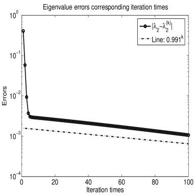
Figure 1: The eigenvalue errors of the shift-inverse method with Richardson iteration step

5 Concluding remarks

In this paper, we discuss the convergence behavior of the shift-inverse method with Richardson iteration step for the eigenvalue problem. It is shown that the eigenvalue gap decide the convergence speed.

References

- [1] H. Chen, Y. He, Y. Li and H. Xie, A multigrid method for eigenvalue problems based on shifted-inverse power technique, European Journal of Mathematics, 1(1) (2015), 207-228.
- [2] Y. Saad, Numerical Methods for Large Eigenvalue Problems, Society for Industral and Applied Mathematics, 2011.
- [3] Y. Notay, Convergence analysis of inexact Rayleigh quotient iteration, SIAM J. Matrix Anal., 24 (2003), 627-644.