A Large-Scale Study of Language Models
for Chord Prediction

Abstract

We conduct a large-scale study of language models for chord prediction. Specifically, we compare $N$-gram models to various flavours of recurrent neural networks on a comprehensive dataset comprising all publicly available datasets of annotated chords known to us. This large amount of data allows us to systematically explore hyper-parameter settings for the recurrent neural networks—a crucial step in achieving good results with this model class. Our results show not only a quantitative difference between the models, but also a qualitative one: in contrast to static $N$-gram models, certain RNN configurations adapt to the songs at test time. This finding constitutes a further step towards the development of chord recognition systems that are more aware of local musical context than what was previously possible.

Index Terms— Language Modelling, Chord Prediction, Recurrent Neural Networks

1 Introduction

Chord recognition is a long-standing topic in the music information retrieval community. Steady advances notwithstanding, results have seemed to stagnate in recent years. The study in [1] offers possible explanations, including invalid harmonic assumptions, limitations of evaluation measures, conflicting problem definitions, and the subjectivity inherent to this task. All of these criticisms are certainly valid, and in our view, the latter two bear the greatest potential to hamper further improvements. However, at present there is still a large performance gap between human annotators (measured via inter-annotator agreement) and automatic systems [1], although they are subjected to the same constraints.

We can divide a chord recognition system into two parts: hearing (acoustic modelling, feature extraction) and understanding (combining observations, finding a meaningful chord sequence). Research has focused mainly on the former by finding better features and acoustic models [2, 3, 4], while only a few works have explored improvements of the latter using temporal models [5, 6, 7]. This trend was reinforced through the insight that existing temporal models do little but smooth the noisy predictions of the acoustic model over time, i.e. they mainly model the chord’s duration [8, 9].

Thus, we suggest another possible explanation for the performance gap: current state-of-the-art chord recognition systems lack a meaningful understanding of harmony and its development in music. As shown in [10], such an understanding can only derive from sequential models that operate at higher temporal levels than those based on audio frames.

The present work addresses this issue by exploring the capabilities of automatically learned chord language models to predict chord sequences. To our knowledge, this paper constitutes the first attempt to systematically find and evaluate such models. We have seen work on optimising low-level and/or Markovian temporal models in e.g. [9], and work on low-level non-Markovian models in e.g. [5], but as argued in [10], at the level of audio frames, there is little to improve upon the current state-of-the-art.

Our work compares recurrent neural networks (RNNs) with higher-order $N$-gram models. We evaluate these models independently based on how well they predict chord sequences. The question on how to integrate them into a complete chord recognition system is left for future work.

2 Data

We compiled a comprehensive set of chord annotations to perform a large-scale evaluation of different language models for chord prediction. To our knowledge, our compound dataset consists of all time-aligned chord annotations that are publicly available. Table 1 provides detailed information about the data. In total, we have $1841$ songs from a variety of genres and decades, with a focus on pop/rock between 1950 and 2000. After we remove duplicate songs and merge consecutive identical annotations, the dataset consists of $1766$ songs containing $161\,796$ unique chord annotations.

Name	Ref.	No. Pieces	No. Chords
Beatles	[11]	180	$12\,646$
Jay Chou	[12]	29	$3356$
McGill Billboard	[13]	742	$70\,197$
Queen	[14]	20	$2265$
Robbie Williams	[15]	65	$6513$
Rock	[16]	201	$18\,343$
RWC	[17]	100	$12\,726$
US Pop 2002	[18]	195	$23\,309$
Weimar Jazz	[19]	291	$18\,179$
Zweieck	[14]	18	$1822$
Total		$1841$	$169\,356$
Unique		$1766$	$161\,796$

Table 1: Individual datasets used to create the compound dataset in this study. For the Rock corpus, we used the annotations by Temperley rather than those by De Clerq.

The dataset is miniscule compared to those available for natural language processing: e.g., the NYT section of the English Gigaword dataset (of which only a subset of 6.4 million words is used in [20] for training language models) consists of 37 million words. Therefore, we leverage domain knowledge to generate additional, semi-artificial chord sequences. Assuming that chord progressions are independent of musical key (as in Roman numeral analysis), and that musical keys are uniformly distributed (a simplifying assumption), we transpose each chord sequence to all possible keys during training. This step increases the amount of training sequences by a factor of 12; however, the artificially created data are highly correlated with the existing data, and thus are not equivalent to truly having 12 times as much data available. We will refer to this process as data augmentation in the remainder of this paper.

We focus on the major/minor chord vocabulary, and follow the standard mapping as described in [9]: chords with a minor 3^rd in the first interval are considered minor, the rest major. This mapping results in a vocabulary of size 25 ($12$ root notes $\times\{\text{maj},\text{min}\}$ and the “no-chord” class). Bearing in mind the reduced vocabulary and the more repetitive nature of chord progressions compared to spoken language, we feel that the size of this dataset after data augmentation is appropriate for training and evaluating models for chord prediction.

3 Experimental Setup

Our experiments evaluate how well various models predict chords. This amounts to measuring the average probability the model assigns to the (correct) upcoming chord symbol, given the ones it has already observed in a sequence. More formally, given a sequence of chords $\bm{y}=(y_{1},\ldots,y_{K})$, the model $M$ yields $P_{M}(y_{k}\mid y_{1}^{k-1})$ for each $k$. (We denote $y_{1},\ldots,y_{k-1}$ as $y_{1}^{k-1}$.) The probability of the complete chord sequence can then be computed as

$$P_{M}\left(\bm{y}\right)=P_{M}(y_{1})\cdot\Pi_{k=2}^{K}P_{M}\left(y_{k}\mid y_{1}^{k-1}\right).$$ (1)

The higher $P_{M}(\bm{y})$, the better $M$ models $\bm{y}$. To measure how well $M$ models all chord sequences in a dataset $\mathcal{Y}$, we next compute the average log-probability assigned to its sequences:

$$\mathcal{L}(M,\mathcal{Y})=\frac{1}{N_{\mathcal{Y}}}\sum_{\bm{y}\in\mathcal{Y}}\log\left(P_{M}\left(\bm{y}\right)\right),$$ (2)

where $N_{\mathcal{Y}}$ is the total number of chord symbols in the dataset. This equation corresponds to the negative cross-entropy between the model’s distribution and the data distribution.

All models are trained and tested on the compound dataset. We use 20% of the data for testing, and 80% for training. 15% of the training data is held out for validation. All splits are stratified by dataset.

4 $N$-Gram Language Models

$N$-gram language models are Markovian probabilistic models that assume a fixed-length history (of length $N-1$) in order to predict the next symbol. Hence, they assume $P_{M}(y_{k}\mid y_{1}^{k-1})=P_{M}(y_{k}\mid y_{k-N+1}^{k-1})$. This fixed-length history allows the probabilities to be stored in a table, with its entries computed using maximum-likelihood estimation (i.e., by counting occurrences in the training set).

With larger $N$, the sparsity of the probability table increases exponentially due to the finite number of $N$-grams in the training set. We solve this problem using Lidstone smoothing, which adds a pseudo-count $\alpha$ to each possible $N$-gram. We determine the value of $\alpha$ for each model using the validation set.

4.1 Model Selection

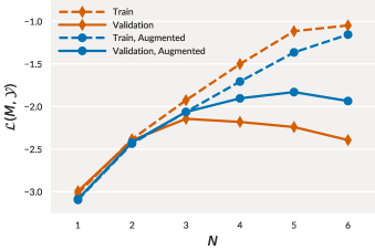
We find the best $N$-gram model by selecting the one with best results on the validation set. To this end, we evaluate models with $N\in\{1,2,3,4,5,6\}$, with and without data augmentation. $N=1$ corresponds to a model that predicts chords just by their frequency in the training data, $N=2$ to a model that could be deployed in a simple first-order Hidden Markov Model.

Figure 1 presents the results of the models on the training and validation sets. With data augmentation, the best result is achieved by a $5$-gram model ($\alpha=0.3$).

Fig. 1: Average log-probability of all evaluated $N$-gram models.

5 Recurrent Neural Language Models

Recurrent Neural Networks (RNNs, see [21] for an overview) are powerful models designed for sequential modelling tasks. In their simplest form, RNNs transform input sequences $\bm{x}_{1}^{K}$ to an output sequence $\bm{o}_{1}^{K}$ through a non-linear projection into a hidden layer $\bm{h}_{1}^{K}$, parameterised by weight matrices $\bm{W}\!_{hx}$, $\bm{W}\!_{hh}$ and $\bm{W}\!_{oh}$:

$$\bm{h}_{k} =\sigma_{h}\left(\bm{W}\!_{hx}\bm{x}_{k}+\bm{W}\!_{hh}\bm{h}_{k-1}\right)$$ (3)

$$\bm{o}_{k} =\sigma_{o}\left(\bm{W}\!_{oh}\bm{h}_{k}\right),$$ (4)

where $\sigma_{h}$ and $\sigma_{o}$ are the activation functions for the hidden layer (e.g. the sigmoid function), and the output layer (e.g. the softmax), respectively. We left out bias terms for simplicity.

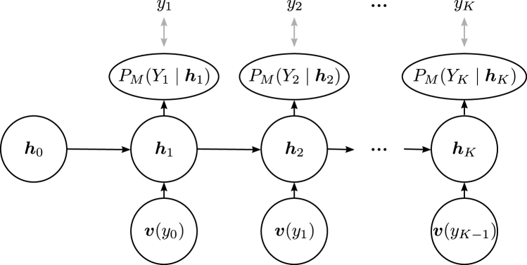
Their use as language models was proposed in [20]. For this purpose, the input at each time step $k$ is a vector representation of the preceding symbol $y_{k-1}$. We call this the chord embedding, and denote it $\bm{v}(y_{k-1})$. In the simplest case, this is a one-hot vector. The network’s output $\bm{o}_{k}$ is then interpreted as the conditional probability over the next chord symbol $P_{M}\left(Y_{k}\mid y_{1}^{k-1}\right)$. During training, the categorical cross-entropy between the $\bm{o}_{k}$ and the true chord symbol is minimised by adapting the weight matrices in Eq. 3 and 4 using stochastic gradient descent and back-propagation through time. Figure 2 provides an overview of the model structure.

Fig. 2: A simple RNN-based language model. We can easily stack more recurrent hidden layers or add skip-connections between the input and each hidden layer or the output.

Each output $\bm{o}_{k}$ depends on all previous inputs $y_{1}^{k-1}$ through the recurrent connection in the hidden layer. This allows the network to consider all previous chords when computing $P_{M}(y_{k}\mid y_{1}^{k-1})$. In practice, this capacity is limited because of the limited size of the hidden layer, and the fragile learning procedure of back-propagation through time, which faces the well-known problems of exploding and vanishing gradients.

5.1 Chord Embeddings

As mentioned earlier, we need to represent chord classes as vectors to use them in the RNN language model framework. In this work, we explore three possibilities: 1) using the one-hot encoding of the class, 2) using a fixed-length vector that is learned jointly with the language model, and 3) learning an embedding using the word2vec skip-gram model [22] before training the language model itself. In this case, the chord embeddings are optimised to predict the neighbouring chords.

5.2 Model Selection

RNNs have more hyper-parameters compared to $N$-gram models: we can set the number of hidden layers, the size of each hidden layer, the type and dimensionality of the input chord embedding, the activation function for each hidden layer, whether to use skip-connections, and finally, we can decide to use simple RNNs or more advanced hidden layer structures such as Long Short-Term Memory (LSTM) [23] or Gated Recurrent Units (GRU) [24]. Additionally, the training procedure has its own hyper-parameters, such as learning rate or mini-batch size. Table 2 presents the hyper-parameter space we sampled from.

Hyper Parameter	Sample Space
Embedding Size	$\{4,8,16,24\}$
Embedding Type	$\{\text{one-hot},\text{word2vec},\text{learned}\}$
No. Hidden Layers	$N_{h}\in\{1,2,3,4,5\}$
Hidden Layer Size	$D_{h}\in\{128,256,512,1024\}$
Skip Connections	$\{\text{yes},\text{no}\}$
Learning Rate	$lr=\begin{cases}\{0.001,0.0005\}&N_{h}\leq 3\\ \{0.0005,0.00025\}&\text{else}\end{cases}$
Learning Rate (GRU)	$lr=\begin{cases}\{0.005,0.001\}&N_{h}\leq 3\\ \{0.001,0.0005\}&\text{else}\end{cases}$

Table 2: Hyper-parameter space we sampled from to find good model configurations for each of the RNN types (simple, LSTM, GRU). Possible learning rate values were determined on a limited number of preliminary experiments.

We fix the following hyper-parameters for all training runs: we apply data augmentation, employ stochastic gradient descent with a batch size of 4 and the ADAM update rule [25], set all hidden layers to the same (but variable) size, and stop training if the validation loss does not improve within 15 epochs.

The large number of hyper-parameters prevents us from conducting an exhaustive search for the optimal architecture. Instead, we use Hyperband [26], a bandit-based black-box hyper-parameter optimisation scheme, to find good configurations for each considered RNN type.

In total, we considered 128 configuration for each RNN type (384 different models). The best RNN setup used one-hot input encoding, skip connections, and $N_{h}=5$, $D_{h}=256$, $lr=2.5e^{-4}$. The best GRU also used one-hot input encoding, but no skip connections, and $N_{h}=3$, $D_{h}=512$, $lr=1e^{-3}$. The best LSTM used a word2vec input encoding with 16 dimensions, skip connections, and $N_{h}=3$, $D_{h}=512$, $lr=1e^{-3}$.

In a final step, we further improve the learned models by a fine-tuning stage. Here, we take the best models found for each RNN type, and re-start training from the epoch that gave the best results on the validation set, but use $\nicefrac{{1}}{{10}}$ of the original learning rate. As shown in Table 3, this step slightly improves the models.

6 Results and Discussion

Fig. 3: $-\mathcal{L}(M,\mathcal{Y})$ (lower is better) of the best model for each model class on the compound test set, and split up into the individual datasets. The numbers in parentheses show the number of chord predictions in each set. Whiskers are 95% confidence intervals computed using bootstrapping. We observe a similar pattern for each set, with the LSTM and GRU performing equally on most of the datasets. We also see that chords are easier to predict in some datasets (e.g. “Rock”), while more difficult in others, (e.g. “RWC”).

Fig. 4: Avg. cumulative log-probability per chord step $L_{\leq}(k;M,\mathcal{Y})$. The predictions of the static 5-gram model worsen over time, which indicates that chord progressions later in the songs deviate more from general patterns than in the beginning. The LSTM and GRU models do not suffer from this problem, however, and predictions even improve after chord 40. We conjecture that these models better remember previously seen chords and patterns, which enables them to automatically adapt as a song progresses.

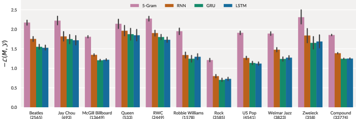
We compare the best model of each RNN type with the 5-gram baseline. To this end, we compute $\mathcal{L}(M,\mathcal{Y})$ according to Eq. 2 on the test set, and present the results in Tab. 3 and Fig. 3. We see the RNN-based models easily outperform the 5-gram model, with the LSTM and GRU models performing best. Statistical significance was determined by a paired t-test with Bonferroni correction.

	5-gram	RNN	GRU	LSTM
Val.	$1.830\,066\,183\,247\,372\,8$	$1.464\,829\,755\,361\,091\,4$	$1.328\,334\,117\,299\,514\,2$	$1.302\,044\,712\,251\,900\,5$
Val. (fine-tuned)	—	$1.417\,442\,732\,083\,965\,3$	$1.289\,725\,684\,678\,890\,3$	$1.272\,035\,605\,365\,961\,4$
Test	$1.874\,272\,648\,308\,856\,3$	$1.386\,799$	$1.243\,915\,0$	$1.248\,633$

Table 3: $-\mathcal{L}(M,\mathcal{Y})$ (lower is better) on the validation and test sets for the best model of each model class. All RNN-based models outperform the 5-gram model, with the GRU yielding the highest avg. log-probability. Statistically equivalent results are marked in bold.

Recurrent neural networks have the capability to remember information over time. We thus call them dynamic models, compared to the static characteristic of standard models based on N-grams. To investigate if the RNN-based language models can leverage this capability, we examine the development of their prediction quality—the log-probability of the correct chord—over the progression of songs.

This is a function of both model capacity and song complexity: given a static model, and repetitive songs that do not change much over time, the log-probabilities assigned to the chords should remain approximately constant; however, if e.g. chords in interludes tend to deviate more from standard chord progressions, static models would yield lower log-probabilities in these cases. On the other hand, if a dynamic model could remember chord progressions from the past, the predictions would improve over time for very repetitive songs.

To evaluate this quantitatively, we first selected from the test set songs that contained at least 100 chords, which left us with 136 pieces. We then computed the average cumulative log-probability of chords up to a position in a song as

$$\mathcal{L}_{\leq}(k;M,\mathcal{Y}) =\frac{1}{k|\mathcal{Y}|}\sum_{\bm{y}\in\mathcal{Y}}\sum_{\tilde{k}=1}^{k}\log\left[P_{M}\left(y_{\tilde{k}}\mid y_{1}^{\tilde{k}-1}\right)\right].$$ (5)

Note that Eq. 5 converges to the objective in Eq. 2 with increasing $k$.

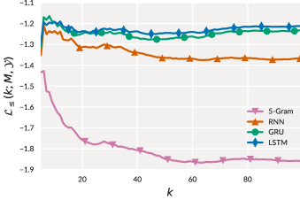
Figure 4 presents the results for each model. To our surprise, the performance of the static 5-gram model drops significantly during the first 20 chords and continues to fall until around chord 60, after which it stagnates. This indicates that the chord progressions in the beginning of the songs are easier to predict by a static model—i.e., more closely follow the general chord progressions the model learned, while those later in the songs deviate more from common patterns.

In comparison, the RNN-based models do not suffer during the first 20 chords. Although they show similar behaviour during the first 20 chords, the LSTM and GRU models also behave differently later in the songs: both the GRU and the LSTM improve from around chord 40, whereas the performance of the simple RNN continues to drop until around chord 60 (similarly to the 5-gram model, but on a higher level).

Since predicting chords later in the songs is more difficult than at the beginning, but the LSTM and the GRU are only negligibly affected by this (they almost recover to their performance at the beginning), we argue that both the GRU and the LSTM models are better capable of adapting to the current song. One explanation for this might be that these models privilege intra-song statistics during prediction. Thus, rather than learning a global, generic model trained on the statistics of an entire corpus, we conjecture that these models also acquire and apply knowledge about the immediate past.

7 Conclusion

We presented a comprehensive evaluation of chord language models, with a focus on RNN-based architectures. We discovered the best performing hyper-parameters, and trained and evaluated the models on a large compound dataset consisting of various genres. Our results show that 1) all RNN-based models outperform $N$-gram models, 2) gated RNN cells such as the LSTM cell or the GRU outperform simple RNNs, and 3) that both LSTM and GRU networks seem to adapt their predictions to what they observed in the past.

We conjecture that to improve the recently stagnant chord recognition results, we need models with a better understanding of music than has been demonstrated in previous state-of-the-art systems. This work is a first step towards this goal. Future research needs to deal with modelling chord durations appropriately, and with integrating such models with frame-wise acoustic chord classifiers.

References

- [1] Eric J. Humphrey and Juan P. Bello, “Four Timely Insights on Automatic Chord Estimation,” in Proceedings of the 16th International Society for Music Information Retrieval Conference (ISMIR), Málaga, Spain, 2015.
- [2] Eric J. Humphrey and Juan P. Bello, “Rethinking Automatic Chord Recognition with Convolutional Neural Networks,” in 11th International Conference on Machine Learning and Applications (ICMLA), Boca Raton, USA, 2012.
- [3] Filip Korzeniowski and Gerhard Widmer, “Feature Learning for Chord Recognition: The Deep Chroma Extractor,” in Proceedings of the 17th International Society for Music Information Retrieval Conference (ISMIR), New York, USA, 2016.
- [4] Yushi Ueda, Yuki Uchiyama, Takuya Nishimoto, Nobutaka Ono, and Shigeki Sagayama, “HMM-based approach for automatic chord detection using refined acoustic features,” in International Conference on Acoustics Speech and Signal Processing (ICASSP), Dallas, USA, 2010.
- [5] Nicolas Boulanger-Lewandowski, Yoshua Bengio, and Pascal Vincent, “Audio chord recognition with recurrent neural networks,” in Proceedings of the 14th International Society for Music Information Retrieval Conference (ISMIR), Curitiba, Brazil, 2013.
- [6] Matthias Mauch and Simon Dixon, “Approximate note transcription for the improved identification of difficult chords,” in Proceedings of the 11th International Society for Music Information Retrieval Conference (ISMIR), Utrecht, Netherlands, 2010.
- [7] Johan Pauwels and Jean-Pierre Martens, “Combining Musicological Knowledge About Chords and Keys in a Simultaneous Chord and Local Key Estimation System,” Journal of New Music Research, vol. 43, no. 3, pp. 318–330, 2014.
- [8] Ruofeng Chen, Weibin Shen, Ajay Srinivasamurthy, and Parag Chordia, “Chord recognition using duration-explicit hidden Markov models,” in Proceedings of the 13th International Society for Music Information Retrieval Conference (ISMIR), Porto, Portugal, 2012.
- [9] Taemin Cho and Juan P. Bello, “On the Relative Importance of Individual Components of Chord Recognition Systems,” IEEE/ACM Transactions on Audio, Speech, and Language Processing, vol. 22, no. 2, pp. 477–492, 2014.
- [10] Filip Korzeniowski and Gerhard Widmer, “On the Futility of Learning Complex Frame-Level Language Models for Chord Recognition,” in Proceedings of the AES International Conference on Semantic Audio, Erlangen, Germany, 2017.
- [11] Christopher Harte, Towards Automatic Extraction of Harmony Information from Music Signals, Dissertation, Department of Electronic Engineering, Queen Mary, University of London, London, United Kingdom, 2010.
- [12] Junqi Deng and Yu-Kwong Kwok, “Automatic Chord estimation on seventhsbass Chord vocabulary using deep neural network,” in International Conference on Acoustics, Speech and Signal Processing (ICASSP), Shanghai, China, 2016.
- [13] John Ashley Burgoyne, Jonathan Wild, and Ichiro Fujinaga, “An Expert Ground Truth Set for Audio Chord Recognition and Music Analysis.,” in Proceedings of the 12th International Society for Music Information Retrieval Conference (ISMIR), Miami, USA, 2011.
- [14] Matthias Mauch, Chris Cannam, Matthew Davies, Simon Dixon, Christopher Harte, Sefki Kolozali, Dan Tidhar, and Mark Sandler, “OMRAS2 metadata project 2009,” in Late Breaking Demo of the 10th International Conference on Music Information Retrieval (ISMIR), Kobe, Japan, 2009.
- [15] Bruno Di Giorgi, Massimiliano Zanoni, Augusto Sarti, and Stefano Tubaro, “Automatic chord recognition based on the probabilistic modeling of diatonic modal harmony,” in Proceedings of the 8th International Workshop on Multidimensional Systems, Erlangen, Germany, 2013.
- [16] Trevor de Clercq and David Temperley, “A corpus analysis of rock harmony,” Popular Music, vol. 30, no. 01, pp. 47–70, 2011.
- [17] Masataka Goto, Hiroki Hashiguchi, Takuichi Nishimura, and Ryuichi Oka, “RWC Music Database: Popular, Classical and Jazz Music Databases.,” in Proceedings of the 3rd International Conference on Music Information Retrieval (ISMIR), Paris, France, 2002.
- [18] Daniel P. W. Ellis, Adam Berenzweig, and Brian Whitman, “The ”uspop2002” Pop Music data set,” https://labrosa.ee.columbia.edu/projects/musicsim/uspop2002.html, 2003.
- [19] The Jazzomat Research Project, “Weimar Jazz Database (WJazzD),” http://jazzomat.hfm-weimar.de/dbformat/dboverview.html, 2016.
- [20] Tomas Mikolov, Martin Karafiát, Lukás Burget, Jan Cernocký, and Sanjeev Khudanpur, “Recurrent neural network based language model,” in INTERSPEECH, Chiba, Japan, 2010.
- [21] Razvan Pascanu, Caglar Gulcehre, Kyunghyun Cho, and Yoshua Bengio, “How to Construct Deep Recurrent Neural Networks,” in Proceedings of the Second International Conference on Learning Representations (ICLR), Banff, Canada, 2014.
- [22] Tomas Mikolov, Kai Chen, Greg Corrado, and Jeffrey Dean, “Efficient estimation of word representations in vector space,” arXiv:1301.3781, 2013.
- [23] Sepp Hochreiter and Jürgen Schmidhuber, “Long Short-Term Memory,” Neural Computation, vol. 9, no. 8, pp. 1735–1780, 1997.
- [24] Kyunghyun Cho, Bart van Merrienboer, Dzmitry Bahdanau, and Yoshua Bengio, “On the Properties of Neural Machine Translation: Encoder-Decoder Approaches,” arXiv:1409.1259, 2014.
- [25] Diederik Kingma and Jimmy Ba, “Adam: A method for stochastic optimization,” arXiv:1412.6980, 2014.
- [26] Lisha Li, Kevin Jamieson, Giulia DeSalvo, Afshin Rostamizadeh, and Ameet Talwalkar, “Hyperband: A Novel Bandit-Based Approach to Hyperparameter Optimization,” arXiv:1603.06560, 2016.