Fingerprint template protection
using minutia-pair spectral representations

Abstract

Storage of biometric data requires some form of template protection in order to preserve the privacy of people enrolled in a biometric database. One approach is to use a Helper Data System. Here it is necessary to transform the raw biometric measurement into a fixed-length representation. In this paper we extend the spectral function approach of Stanko and Škorić [18], which provides such a fixed-length representation for fingerprints. First, we introduce a new spectral function that captures different information from the minutia orientations. It is complementary to the original spectral function, and we use both of them to extract information from a fingerprint image. Second, we construct a helper data system consisting of zero-leakage quantisation followed by the Code Offset Method. We show empirical data which demonstrates that applying our helper data system causes only a small performance penalty compared to fingerprint authentication based on the unprotected spectral functions.

I Introduction

I-A Biometric template protection

Biometric authentication has become popular because of its convenience. Biometrics cannot be forgotten or left at home. Although biometric data is not exactly secret (we are leaving a trail of fingerprints, DNA etc.), it is important to protect biometric data for privacy reasons. Unprotected storage of biometric data could reveal medical conditions and would allow cross-matching of entries in different databases. Large-scale availability of unprotected biometric data would make it easier for malevolent parties to leave misleading traces at crime scenes (e.g. artificial fingerprints [13], synthesized DNA [8].) One of the easiest ways to properly protect a biometric database against breaches and insider attacks (scenarios where the attacker has access to decryption keys) is to store biometrics in hashed form, just like passwords. An error-correction step has to be added to get rid of the measurement noise. To prevent critical leakage from the error correction redundancy data, one uses a Helper Data System (HDS) [11], [5], [17], for instance a Fuzzy Extractor or a Secure Sketch [10], [6], [3]. The best known and simplest HDS scheme is the code-offset method (COM). The COM utilizes a linear binary error-correction code and thus requires a fixed-length representation of the biometric measurement. Such a representation is not straightforward when the measurement noise can cause features of the biometric to appear/disappear. For instance, some minutiae may not be detected in every image captured from the same finger.

A fixed-length representation called spectral minutiae was introduced by Xu et al. [24], [21], [22], [23]. For every detected minutia of sufficient quality, the method evaluates a Fourier-like spectral function on a fixed-size two-dimensional grid; the contributions from the different minutiae are added up. Disappearance of minutiae or appearance of new ones does not affect the size of this representation.

One of the drawbacks of Xu et al.’s construction is that phase information is discarded in order to obtain translation invariance. Nandakumar [14] proposed a variant which does not discard the phase information. However, it reveals personalised reliability data, which makes it difficult to use in a privacy-preserving scheme.

A minutia-pair based variant of Xu et al.’s technique was introduced in [18]. It has a more compact grid and reduced computation times. Minutia pairs (and even triplets) were used in [7, 9], but with a different attacker model that allows encryption keys to exist that are not accessible to the attacker.

I-B Contributions and outline

First we extend the pair-based spectral minutiae method [18] by introducing a new spectral function that captures different information from the minutia orientations. Then we use the spectral functions as the basis for a template protection system. Our HDS consists of two stages. In the first stage, we discretise the analog spectral representation using a zero-leakage HDS [5, 17]. This first HDS reduces quantisation noise, and the helper data reveals no information about the quantised data. Discretisation of the spectral functions typically yields only one bit per grid point. We concatenate the discrete data from all the individual grid points into one long bitstring. In the second stage we apply the Code Offset Method. Our code of choice is a Polar code, because Polar code are low-complexity capacity-achieving codes with flexible rate.

We present False Accept vs. False Reject tradeoffs at various stages of the data processing. We introduce the ‘superfinger’ enrollment method, in which we average the spectral functions from multiple enrollment images. By combining three enrollment images in this way, and constructing a polar code specifically tuned to the individual bit error rate of each bit position, we achieve an Equal Error Rate around 1% for a high-quality fingerprint database, and around 6% for a low-quality database.

The outline of the paper is as follows. In Section II we introduce notation briefly review helper data systems, the spectral minutiae representation, and polar codes. In Section III we introduce the new spectral function. In Section IV we explain our experimental approach and motivate certain design choices such as the number of discretisation intervals and the use of a Gaussian approximation. We introduce two methods for averaging enrollment images.

Section V contains our results, mostly in the form of ROC curves. In Section VI we discuss the results and identify topics for future work.

II Preliminaries

II-A Notation and terminology

We use capitals to represent random variables, and lowercase for their realizations. Sets are denoted by calligraphic font. The set $\mathcal{S}$ is defined as $\mathcal{S}=\{0,\ldots,N-1\}$. The mutual information (see e.g. [4]) between $X$ and $Y$ is $I(X;Y)$. The probability density function (pdf) of the random variable $X\in\mathbb{R}$ in written as $f(x)$ and its cumulative distribution function (cdf) as $F(x)$. We denote the number of minutiae found in a fingerprint by $Z$. The coordinates of the $j$’th minutia are ${\boldsymbol{x}}_{j}=(x_{j},y_{j})$ and its orientation is $\theta_{j}$. We write $\boldsymbol{x}=(\boldsymbol{x}_{j})_{j=1}^{Z}$ and $\boldsymbol{\theta}=(\boldsymbol{\theta}_{j})_{j=1}^{Z}$ We will use the abbreviations FRR = False Reject Rate, FAR = False Accept Rate, EER = Equal Error Rate, ROC = Receiver Operating Characteristic. Bitwise xor of binary strings is denoted as $\oplus$.

II-B Helper Data Systems

A HDS is a cryptographic primitive that allows one to reproducibly extract a secret from a noisy measurement. A HDS consist of two algorithms: Gen (generation) and Rec (reconstruction), see Fig. 1. The Gen algorithm takes a measurement $X$ as input and generates the secret $S$ and a helper data $W$. The Rec algorithm has as input a noisy measurement $Y$ and the helper data; it outputs an estimator $\hat{S}$. If $Y$ is sufficiently close to $X$ then $\hat{S}=S$. The helper data should not reveal much about $S$. Ideally it holds that $I(W;S)=0$. This is known as Zero Leakage helper data.

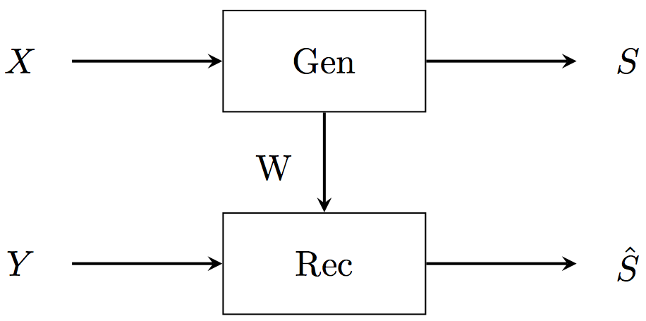
Figure 1: Data flow in a generic Helper Data System.

II-C Two-stage HDS template protection scheme

Fig. 2 shows the two-stage HDS architecture mentioned in Section I-B. The enrollment measurement $x$ is transformed to the spectral representation $(x_{i})_{i=1}^{M}$ on $M$ grid points. The first-stage enrollment procedure Gen1 is applied to each $x_{i}$ individually, yielding short (mostly one-bit) secrets $s_{i}$ and zero-leakage helper data $w_{i}$. The $s_{1}\ldots s_{M}$ are concatentated into a string $k$. Residual noise in $k$ is dealt with by the second-stage HDS (Code Offset Method), whose Gen2 produces a secret $c$ and helper data $r$. A hash $h(c||z)$ is computed, where $z$ is salt. The hash and the salt are stored.

In the verification phase, the noisy $y$ is processed as shown in the bottom half of Fig. 2. The reconstructed secret $\hat{c}$ is hashed with the salt $z$; the resulting hash is compared to the stored hash.

Figure 2: Two-stage Helper Data System.

II-D Minutia-pair spectral representation

Minutiae are special features in a fingerprint, e.g. ridge endings and bifurcations. We briefly describe the minutia-pair spectral representation introduced in [18]. For minutia indices $a,b\in\{1,\ldots,Z\}$ the distance and angle between these minutiae are given by $R_{ab}=|{\bf x}_{a}-{\bf x}_{b}|$ and $\tan\phi_{ab}=\frac{y_{a}-y_{b}}{x_{a}-x_{b}}$. The spectral function $\cal M_{\boldsymbol{x\theta}}$ is defined as

$$\mathcal{M}_{\boldsymbol{x\theta}}(q,R)=\sum_{a=1}^{Z}\sum_{b=a+1}^{Z}e^{iq\phi_{ab}}e^{-\frac{(R-R_{ab})^{2}}{2\sigma^{2}}}e^{i(\theta_{b}-\theta_{a})},$$ (1)

where $\sigma$ is a width parameter. The spectral function is evaluated on a discrete $(q,R)$ grid. The variable $q$ is integer and can be interpreted as the Fourier conjugate of an angular variable, i.e. a harmonic. The function $\cal M_{\boldsymbol{x\theta}}$ is invariant under translations of $\boldsymbol{x}$. When a rotation of the whole fingerprint image is applied over an angle $\delta$, the spectral function transforms in a simple way,

$$\mathcal{M}_{\boldsymbol{x\theta}}(q,R)\to e^{iq\delta}\mathcal{M}_{\boldsymbol{x\theta}}(q,R).$$ (2)

II-E Zero Leakage Helper Data Systems

We briefly review the ZLHDS developed in [5, 17] for quantisation of an enrollment measurement $X\in\mathbb{R}$. The density function of $X$ is $f$, and the cumulative distribution function is $F$. The verification measurement is $Y$. The $X$ and $Y$ are considered to be noisy versions of an underlying ‘true’ value. They have zero mean and variance $\sigma_{X}^{2}$, $\sigma_{Y}^{2}$, respectively. The correlation between $X$ and $Y$ can be characterised by writing $Y=\lambda X+V$, where $\lambda\in[0,1]$ is the attenuation parameter and $V$ is zero-mean noise independent of $X$, with variance $\sigma_{V}^{2}$. It holds that $\sigma^{2}_{Y}=\lambda\sigma^{2}_{X}+\sigma^{2}_{V}$. We consider the identical conditions case: the amount of noise is the same during enrollment and reconstruction. In this situation we have $\sigma^{2}_{X}=\sigma^{2}_{Y}$ and $\lambda^{2}=1-\frac{\sigma^{2}_{V}}{\sigma^{2}_{X}}$.

The real axis $\mathbb{R}$ is divided into $N$ intervals ${\cal A}_{\alpha}=(\Omega_{\alpha},\Omega_{\alpha+1})$, with $\alpha\in\cal S$, ${\cal S}=\{0,\ldots,N-1\}$. Let $p_{\alpha}=\Pr[X\in{\cal A}_{\alpha}]$. The quantisation boundaries are given by $\Omega_{\alpha}=F^{\rm inv}(\sum_{j=0}^{\alpha-1}p_{j})$. The Gen algorithm produces the secret $s$ as $s={\rm max}\{\alpha\in\mathcal{S}:x\geq\Omega_{\alpha}\}$ and the helper data $w\in[0,1)$ as $w=[F(x)-\sum_{j=0}^{s-1}p_{j}]/p_{s}$. The inverse relation, for computing $x$ as a function of $s$ and $w$, is given by $\xi_{s,w}=F^{\rm inv}(\sum_{j=0}^{s-1}p_{j}+wp_{s})$.

The Rec algorithm computes the estimator $\hat{s}$ as the value in $\cal S$ for which it holds that $y\in(\tau_{\hat{s},w},\tau_{\hat{s}+1,w})$, where the parameters $\tau$ are decision boundaries. In the case of Gaussian noise these boundaries are given by

$$\tau_{\alpha,w}=\lambda\frac{\xi_{\alpha-1,w}+\xi_{\alpha,w}}{2}+\frac{\sigma_{V}^{2}\ln\frac{p_{\alpha-1}}{p_{\alpha}}}{\lambda(\xi_{\alpha,w}-\xi_{\alpha-1,w})}.$$ (3)

Here it is understood that $\xi_{-1,w}=-\infty$ and $\xi_{N,w}=\infty$, resulting in $\tau_{0,w}=-\infty$, $\tau_{N,w}=\infty$.

The above scheme ensures that $I(W;S)=0$ and that the reconstruction errors are minimized.

II-F The Code Offset Method (COM)

We briefly describe how the COM is used as a Secure Sketch. Let $C$ be a linear binary error correcting code with message space $\{0,1\}^{m}$ and codewords in $\{0,1\}^{n}$. It has an encoding ${\tt Enc}$: $\{0,1\}^{m}\to\{0,1\}^{n}$, a syndrome function $\tt Syn$: $\{0,1\}^{n}\to\{0,1\}^{n-m}$ and a syndrome decoder $\tt SynDec$: $\{0,1\}^{n-m}\to\{0,1\}^{n}$. In Fig. 2 the Gen2 computes the helper data $r$ as $r={\tt Syn}\,k$. The $c$ in Fig. 2 is equal to $k$. The Rep2 computes the reconstruction $\hat{k}=k^{\prime}\oplus{\tt SynDec}(r\oplus{\tt Syn}\,k^{\prime})$.

II-G Polar codes

Polar codes, proposed by Arıkan [2], are a class of linear block codes that get close to the Shannon limit even at small code length. They are based on the repeated application of the polarisation operation $\Big{(}\begin{matrix}1&0\\ 1&1\end{matrix}\Big{)}$ on two bits of channel input. Applying this operation creates two virtual channels, one of which is better than the original channel and one worse. For $n$ channel inputs, repeating this procedure in the end yields $m$ near-perfect virtual channels, with $m/n$ close to capacity, and $n-m$ near-useless channels. The $m$-bit message is sent over the good channels, while the bad ones are ‘frozen’, i.e used to send a fixed string known a priori by the recipient.

The most popular decoder is the Successive Cancellation Decoder (SCD), which sequentially estimates message bits $(c_{i})_{i=1}^{m}$ according to the frozen bits and the previously estimated bits $\hat{c}_{i-1}$. Polar codes have been recently adopted for the next generation wireless standard (5G), especially for control channels, which have short block length ($\leq 1024$).

III A new spectral function

Figure 3: The relevant angles in a minutia pair.

Consider Fig. 3 (modified from [20]). The invariant angle $\beta_{a}$ is defined as the angle from the orientation of minutia $a$ to the connecting line $ab$, taken in the positive direction. (The $\beta_{b}$ is defined analogously). Modulo $2\pi$ it holds that $\theta_{a}+\beta_{a}=\phi_{ab}$ and $\theta_{b}+\beta_{b}=\phi_{ab}+\pi$. The spectral function (1) uses only the invariant angle $\beta_{a}-\beta_{b}+\pi=\theta_{b}-\theta_{a}$. The second invariant angle, which can be written e.g. as $\pi-\beta_{a}-\beta_{b}=\theta_{a}+\theta_{b}-2\phi_{ab}$, is not used. We therefore now introduce a new spectral function, denoted as $\mathcal{M}_{x\beta}$, which incorporates the invariant angle $\pi-\beta_{a}-\beta_{b}$.

$$\mathcal{M}_{\boldsymbol{x\beta}}(q,R)=\sum_{a=1}^{Z}\sum_{b=a+1}^{Z}e^{i\phi_{ab}(q-2)}e^{-\frac{(R-R_{ab})^{2}}{2\sigma^{2}}}e^{i(\theta_{b}+\theta_{a})}.$$ (4)

We will use $\mathcal{M}_{x\theta}$, $\mathcal{M}_{x\beta}$ and their fusion.

IV Experimental approach

IV-A Databases

We use the MCYT, FVC2000, and FVC2002 database. The MCYT database [15] contains good-quality images from 100 individuals: 10 fingers per individual and 12 images per finger. FVC2000 and FVC2002 contain low-quality images (only index and middle fingers [12]). Each FVC database contains 100 fingers, 8 images per finger. In FVC2002, images number 3, 4, 5, and 6 have an exceptionally large angular displacement, so they are omitted from the experiments.

We extract the minutia position and orientation $(x_{j},y_{j},\theta_{j})$ by using VeriFinger software [1]. For MCYT we evaluate the spectral functions on the same grid as [18], namely $R\in\{16,22,28,\ldots,130\}$ and $q\in\{1,2,\ldots,16\}$ and we maintain $\sigma=2.3$ pixels. For the FVC databases we use the same grid, and $\sigma=3.2$ pixels turns out to be a good choice. The average number of minutiae that can be reliably found is $Z=35$.

IV-B No image rotation

As mentioned in [18], during the reconstruction procedure one can try different rotations of the verification image, but it results only in a minor improvement of the EER. For this reason we do not apply image rotation.

IV-C Quantization methods

Before quantization all spectral functions are normalized to zero mean and unit variance, where the variance is taken of the real and imaginary part together. We quantize the real and imaginary part of the spectral functions separately. We study two methods: ‘hard thresholding’ (without helper data) and the Zero Leakage quantisation of Section II-B. The hard thresholding gives a bit value ‘1’ if ${\rm Re}\,M>0$ and ‘0’ otherwise. We will show results for this method mainly to demonstrate the advantages of Zero Leakage quantisation.

IV-D Gaussian probability distributions

When using the ZLHDS formulas we will assume that the spectral functions are Gaussian-distributed. Figs. 4 and 5 illustrate that this assumption is not far away from the truth.

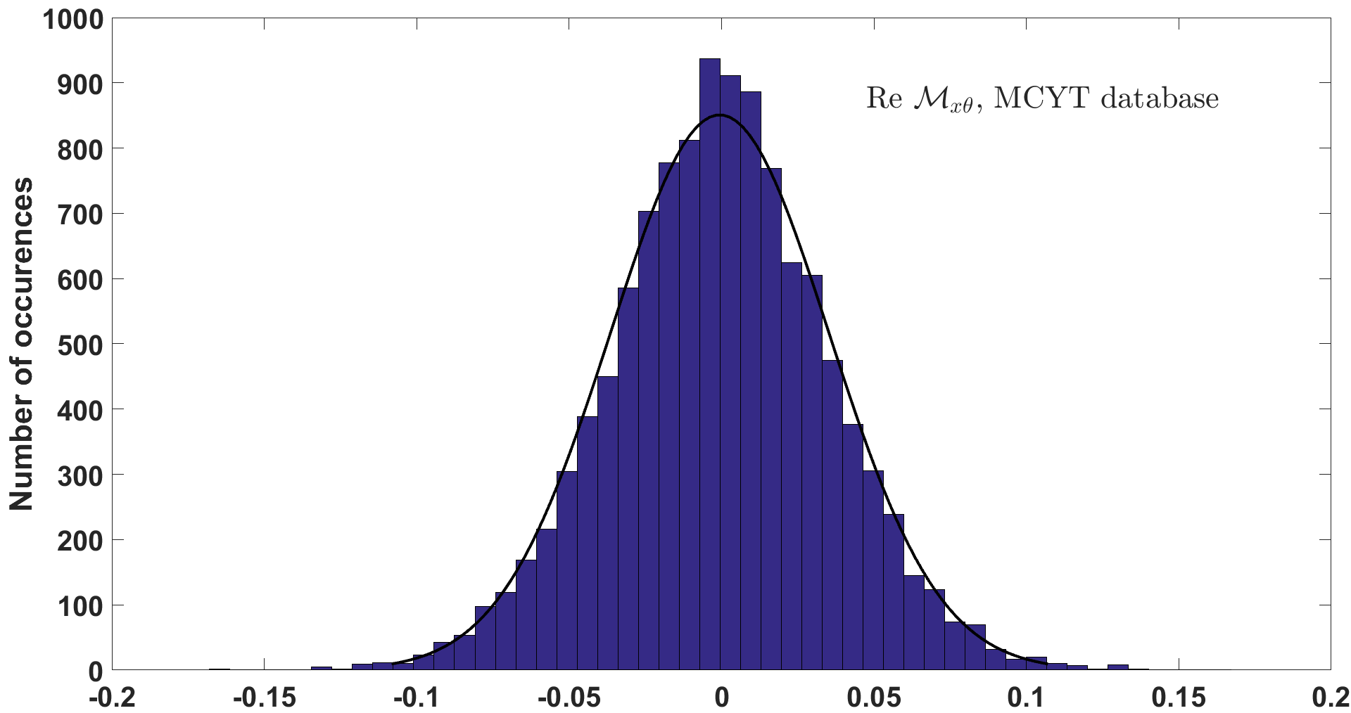
Figure 4: Histogram of ${\rm Re}\,\mathcal{M}_{x\theta}$, and a fitted Gaussian.

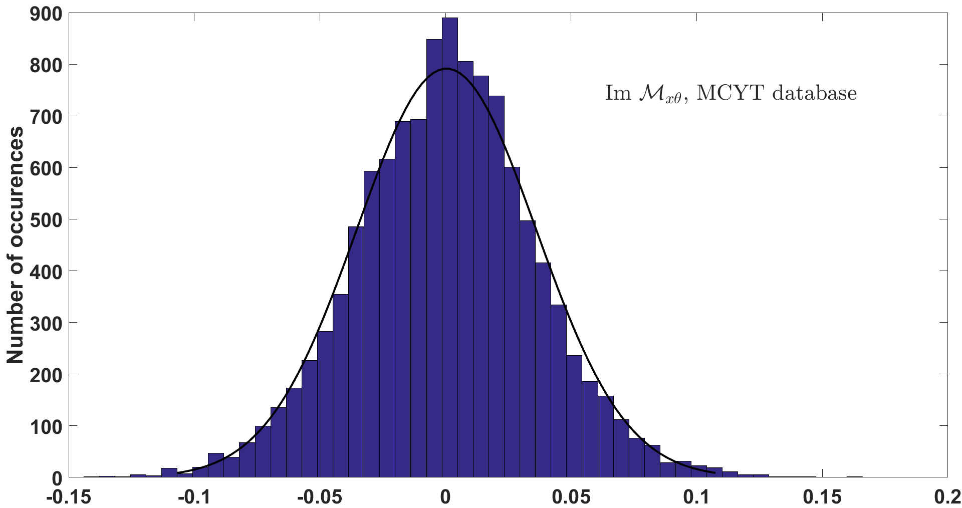
Figure 5: Histogram of ${\rm Im}\,\mathcal{M}_{x\theta}$, and a fitted Gaussian.

IV-E Zero leakage quantization

IV-E1 Signal to noise ratio; setting $N$

In the ZL HDS of Section II-E, the optimal choice of the parameter $N$ (number of quantization intervals) depends on the signal to noise ratio. Fig. 6 shows a comparison between $N=2$ and $N=3$. At low noise it is obvious that $N=3$ extracts more information from the source than $N=2$. At $\sigma_{V}/\sigma_{X}$ larger than approximately $0.3$, there is a regime where $N=3$ can extract more in theory, but is hindered in practice by the high bit error rate. At $\sigma_{V}/\sigma_{X}>0.55$ the $N=2$ ‘wins’ in all respects.

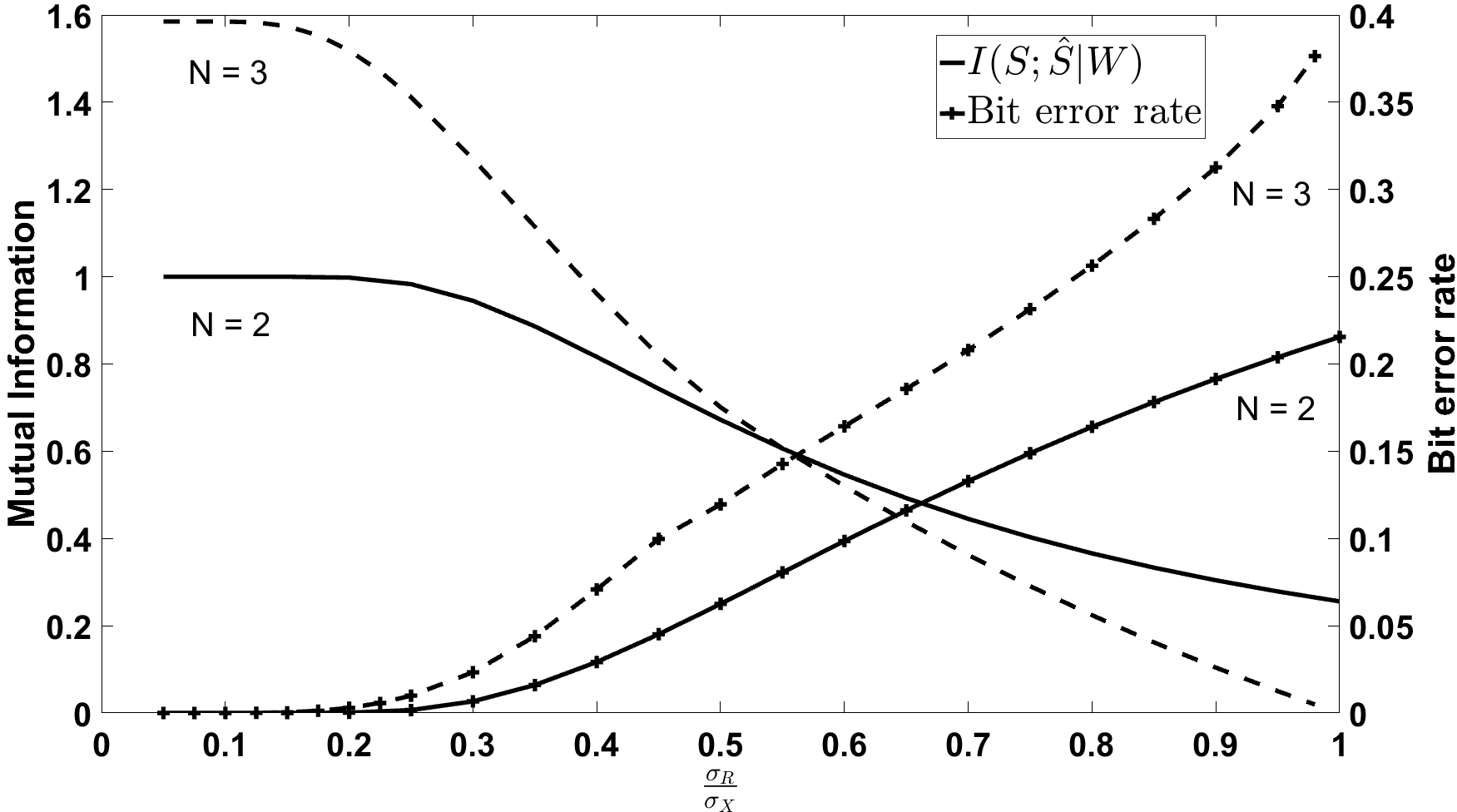
Figure 6: Comparison of ZLHDS with $N=2$ versus $N=3$. Lines without markers: Mutual information between the enrolled key $S$ and the reconstructed key $\hat{S}$ given helper data $W$, as a function of $\sigma_{V}/\sigma_{X}$. Markers: bit error rate as a function of $\sigma_{V}/\sigma_{X}$. The curves follow equations (22) and (26) from [18].

For our data set, we define a $\sigma_{X}^{2}(q,R)$ for every grid point $(q,R)$ as the variance of ${\cal M}(q,R)$ over all images in the database. The noise $\sigma_{V}^{2}(q,R)$ is the variance over all available images of the same finger, averaged over all fingers.

Figs. 7 and 8 show the noise-to-signal ratio. Note the large amount of noise; even the best grid points have $\sigma_{V}/\sigma_{X}>0.45$. Fig. 6 tells us that setting $N=2$ is the best option, and this is the choice we make. At $N=2$ we extract two bits per grid point from each spectral function (one from ${\rm Re}\,{\mathcal{M}}$, one from ${\rm Im}\,{\mathcal{M}}$). Hence our bit string string $k$ (see Fig. 2) derived from ${\mathcal{M}}_{x\theta}$ has length 640. When we apply fusion of ${\mathcal{M}}_{x\theta}$ and ${\mathcal{M}}_{x\beta}$ this becomes 1280.

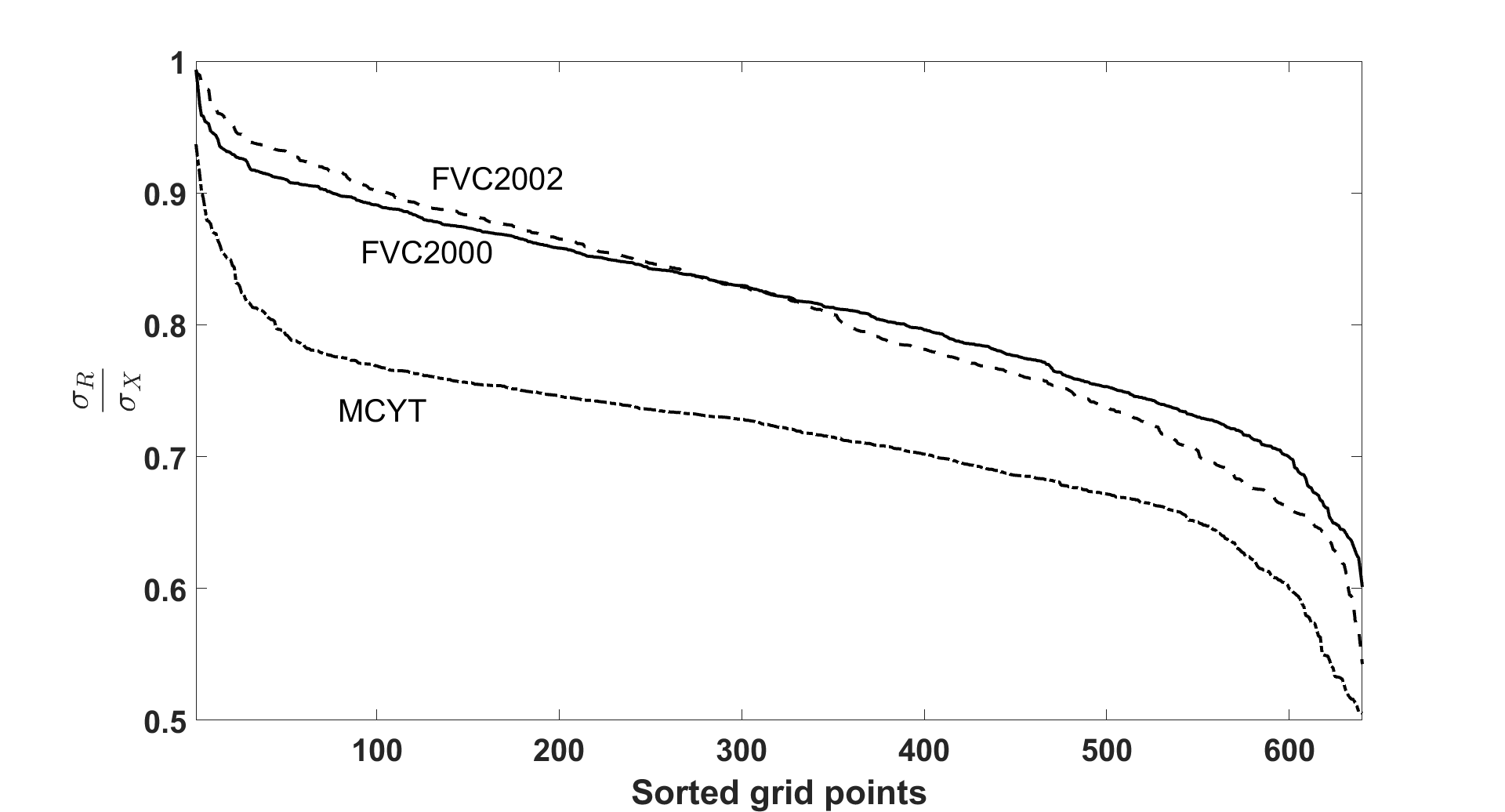
Figure 7: Sorted noise-to-signal ratio of $\mathcal{M}_{x\theta}$ for different databases.

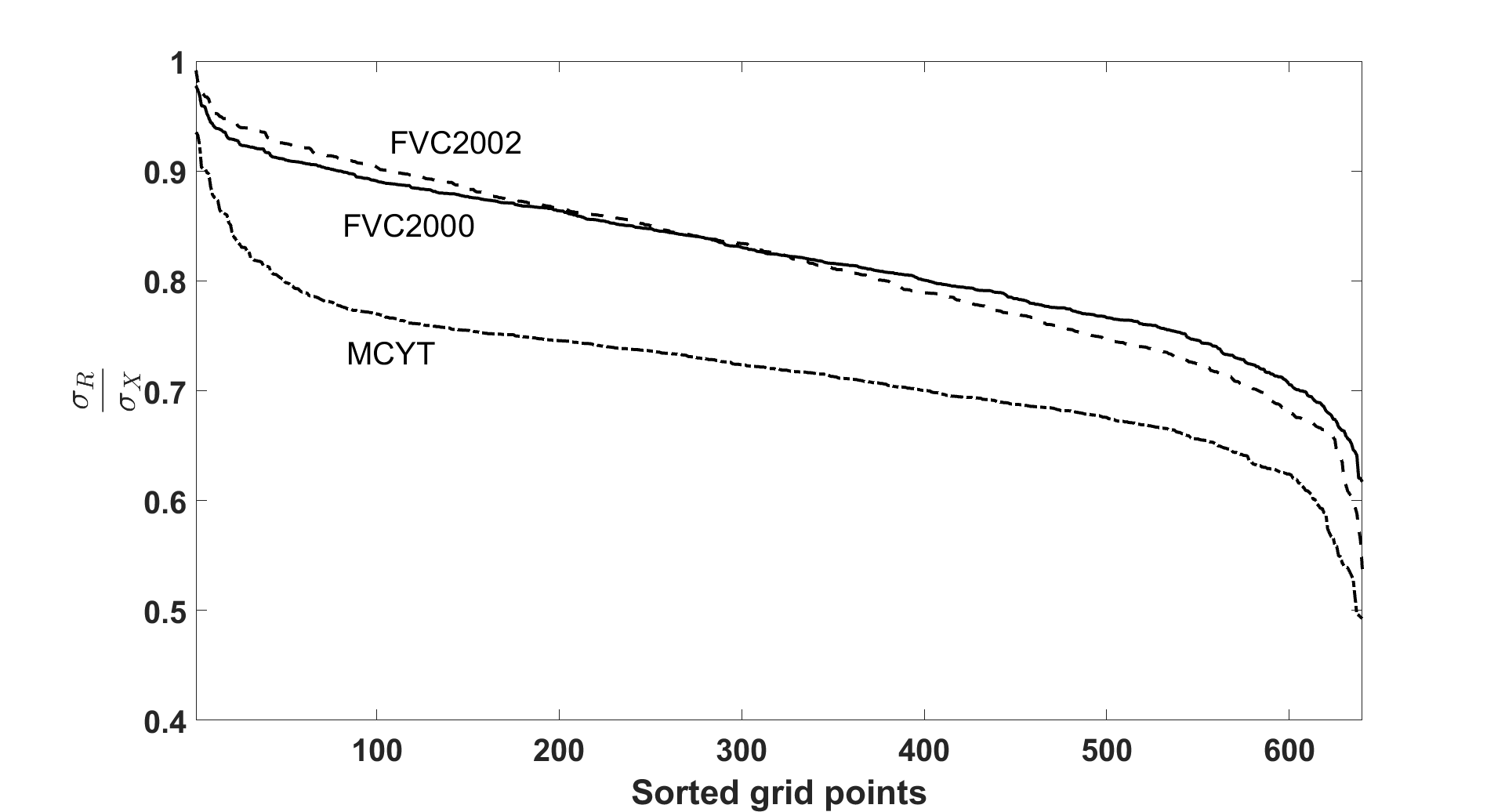
Figure 8: Sorted noise-to-signal ratio of $\mathcal{M}_{x\beta}$ for different databases.

For $N=2$ the formulas in Section II-E simplify to ${\cal A}_{0}=(-\infty,0)$, ${\cal A}_{1}=[0,\infty)$, $p_{0}=p_{1}=\frac{1}{2}$, $\xi_{0,w}=F^{\rm inv}(\frac{w}{2})$, $\xi_{1,w}=F^{\rm inv}(\frac{1}{2}+\frac{w}{2})$, $\tau_{1,w}=\frac{\lambda}{2}(\xi_{0,w}+\xi_{1,w})$. Since we work with Gaussian distributions, $F$ is the Gaussian cdf (‘probability function’).

IV-E2 Enrollment and reconstruction

We have experimented with three different enrollment methods:
E1. A single image is used.
E2: We take the first $t$ images of a finger and calculate the average spectral function. We call this the ‘superfinger’ method. In the ZLHDS calculations the signal-to-noise ratio of the average spectral function is used.

E3: For each of $t$ images we calculate an enrollment string $k$. We apply bitwise majority voting on these strings. (This requires odd $t$.) The reconstruction boundaries are calculated based on the superfinger method, i.e. as in E2.

Reconstruction:
We study fingerprint authentication with genuine pairs and impostor pairs. For pedagogical reasons we will present results at each stage of the signal processing: (1) spectral function domain, before quantisation; (2) binarized domain, without HDS; (3) with ZLHDS; (4) with ZLHDS and discarding the highest-noise grid points.

In the spectral function domain the fingerprint matching is done via a correlation score [18]. In the binarized domain we look at the Hamming weight between the enrolled $k$ and the reconstructed $\hat{k}$. For all cases we will show ROC curves in order to visualise the FAR-FRR tradeoff as a function of the decision threshold.

Let the number of images per finger be denoted as $M$, and the number of fingers in a database as $L$ .

E1: For the spectral domain and the quantization without HDS we compare all genuine pairs, i.e. ${M\choose 2}$ image pairs per finger, resulting in $L{M\choose 2}$ data points. For ZLHDS the number is twice as large, since there is an asymmetry between enrollment and reconstruction. For the FVC databases we generate all possible impostor combinations (all images of all impostor fingers), resulting in ${\cal O}(M^{2}L^{2})$ data points.

For the MCYT database, which is larger, we take only one random image per impostor finger, resulting in ${\cal O}(ML^{2})$ data points.
E2+E3: For genuine pairs we compare the superfinger to the remaining $M-t$ images. Thus we have $(M-t)L$ data points. Impostor pairs are generated as for E1.

Note: The VeriFinger software was not able to extract information for every image.

V Experimental results

V-A FAR/FRR rates before error correction

For each the data processing steps/options before application of the Code Offset method, we investigate the False Accept rates and False Reject rates. We identify a number of trends.

• Figs. 9 and 10 show ROC curves. All the non-analog curves were made under the implicit assumption that for each decision threshold (number of bit flips) an error-correcting code can be constructed that enforces that threshold, i.e. decoding succeeds only if the number of bit flips is below the threshold. Unsurprisingly, we see in the figures that quantisation causes a performance penalty. Furthermore the penalty is clearly less severe when the ZLHDS is used. Finally, it is advantageous to discard some grid points that have bad signal-to-noise ratio. For the curves labeled ‘ZLHDS+reliable components’ only the least noisy 512 bits of $k$ were kept (1024 in the case of fusion). Our choice for the number 512 is not entirely arbitrary: it fits error-correcting codes. Note in Fig. 10 that ZLHDS with reliable component selection performs better than analog spectral functions without reliable component selection. (But not better than analog with selection.)

• The E2 and E3 enrollment methods perform better than E1. Furthermore, performance increases with $t$. A typical example is shown in Fig. 11.

• The spectral functions ${\cal M}_{x\theta}$ and ${\cal M}_{x\beta}$ individually have roughly the same performance. Fusion yields a noticeable improvement. An example is shown in Fig. 12. (We implemented fusion in the analog domain as addition of the two similarity scores.)

• Tables I to V show Equal Error Rates and Bit Error Rates. We see that enrollment methods E2 and E3 have similar performance, with E2 yielding a somewhat lower genuine-pair BER than E3.

• In Table I it may look strange that the EER in the rightmost column is sometimes lower than in the ‘analog’ column. We think this happens because there is no reliable component selection in the ‘analog’ procedure.

• Ideally the impostor BER is 50%. In the tables we see that the impostor BER can get lower than 50% when the ZLHDS is used and the enrollment method is E2. On the other hand, it is always around 50% in the ‘No HDS’ case. This seems to contradict the Zero Leakage property of the helper data system. The ZLHDS is supposed not to leak, i.e. the helper data should not help impostors. However, the zero-leakage property is guaranteed to hold only if the variables are independent. In real-life data there are correlations between grid points and correlations between the real and imaginary part of a spectral function.

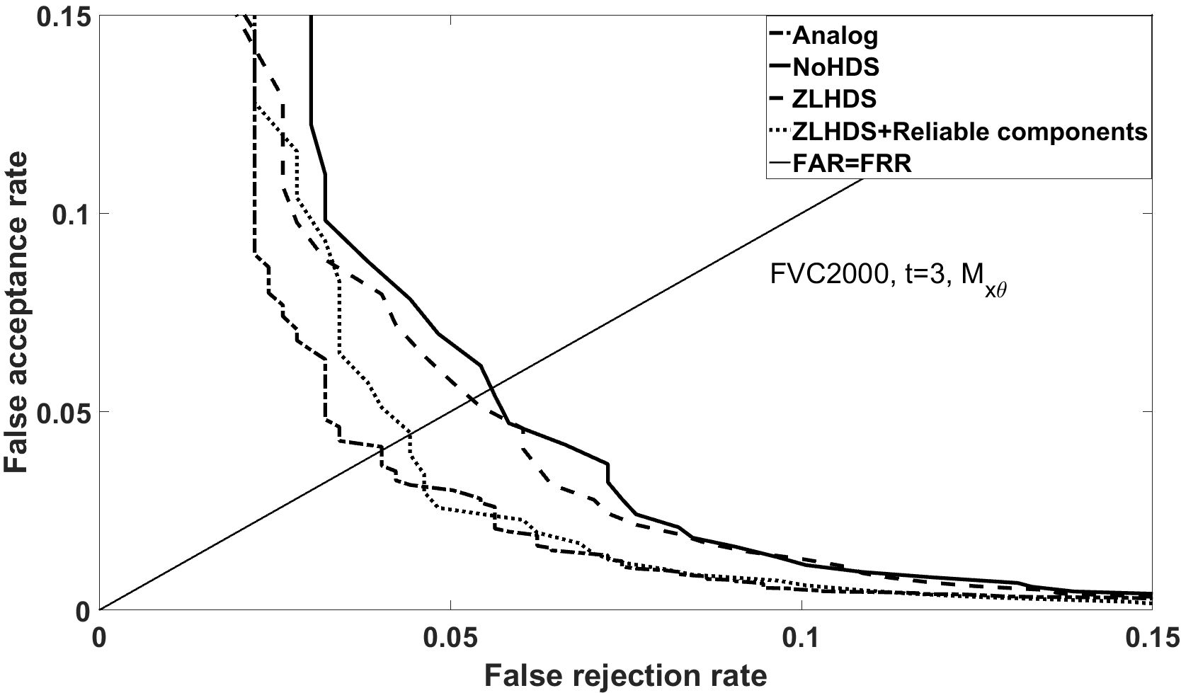
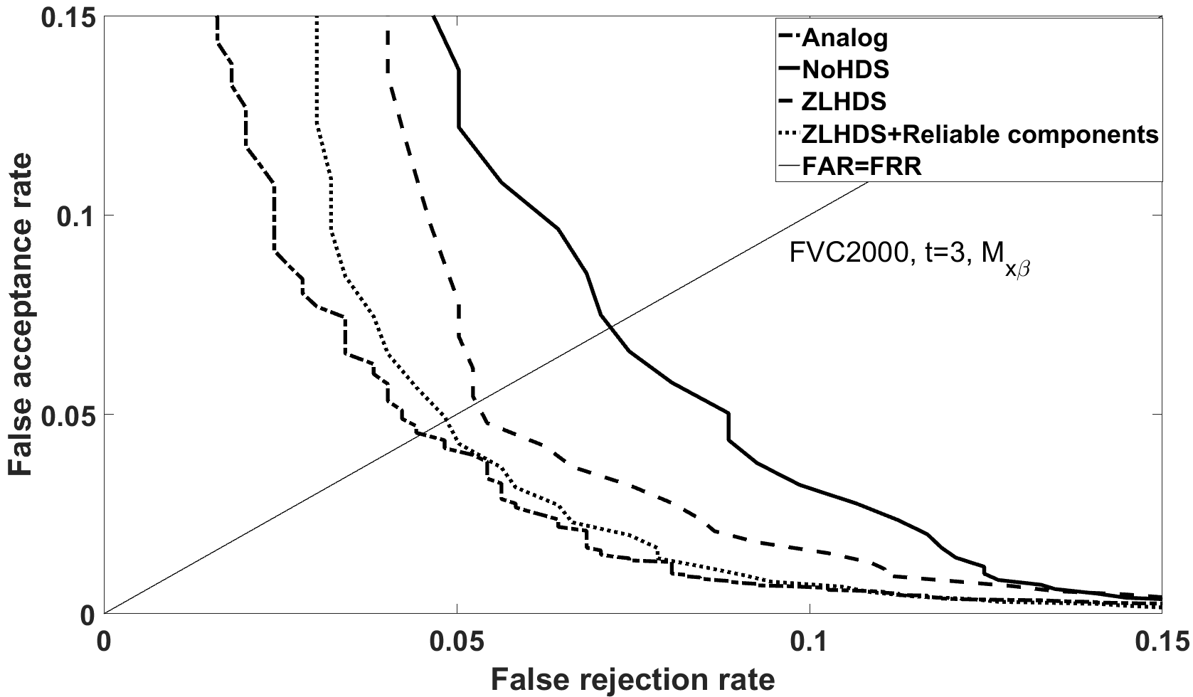
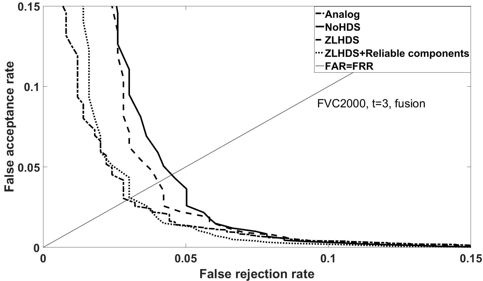
Figure 9: Performance result for several processing methods. FVC2000. Enrollment method E2 with $t=3$.

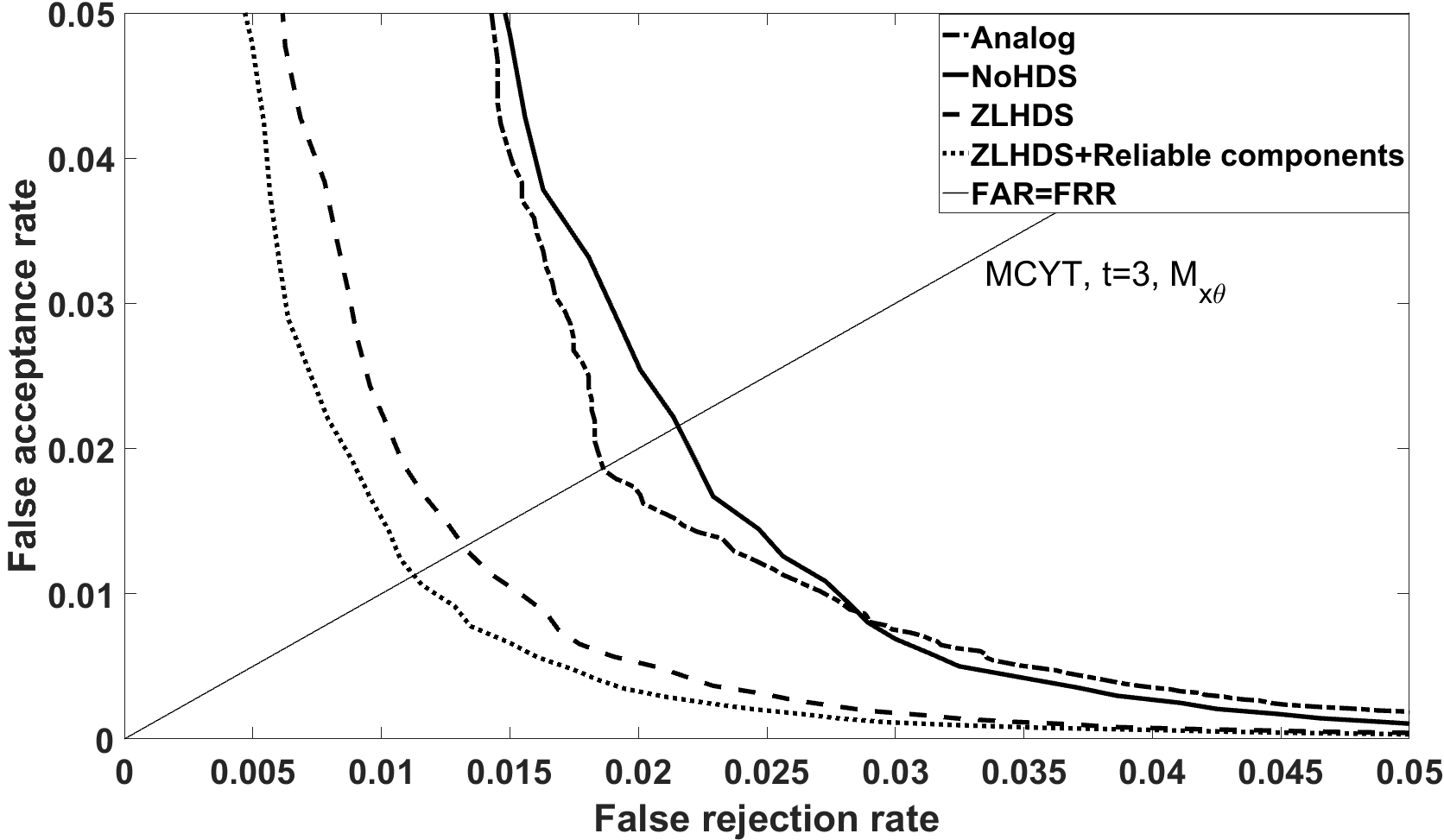
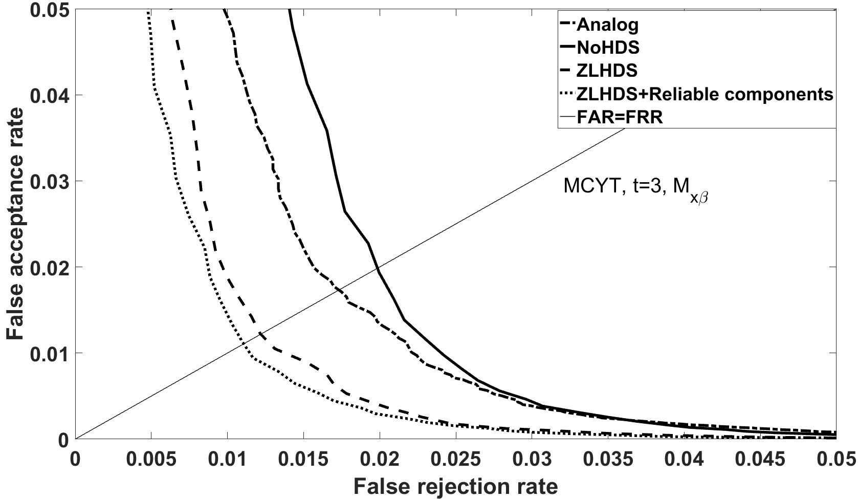
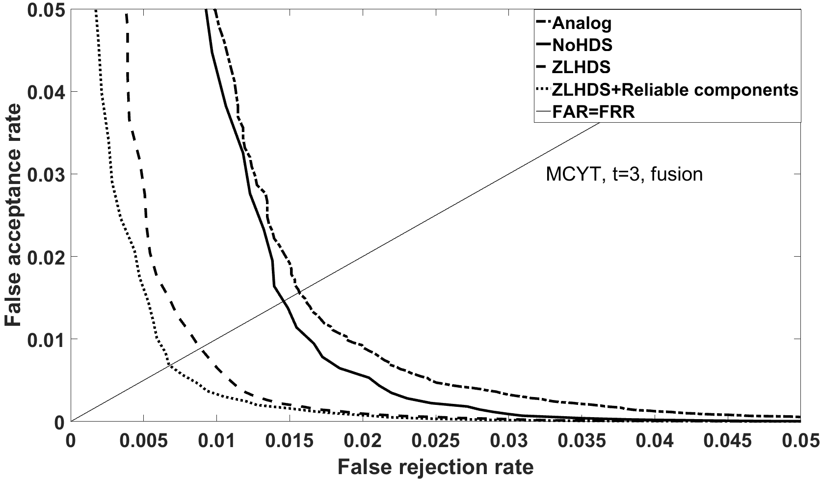
Figure 10: Performance result for several processing methods. MCYT. Enrollment method E2 with $t=3$.

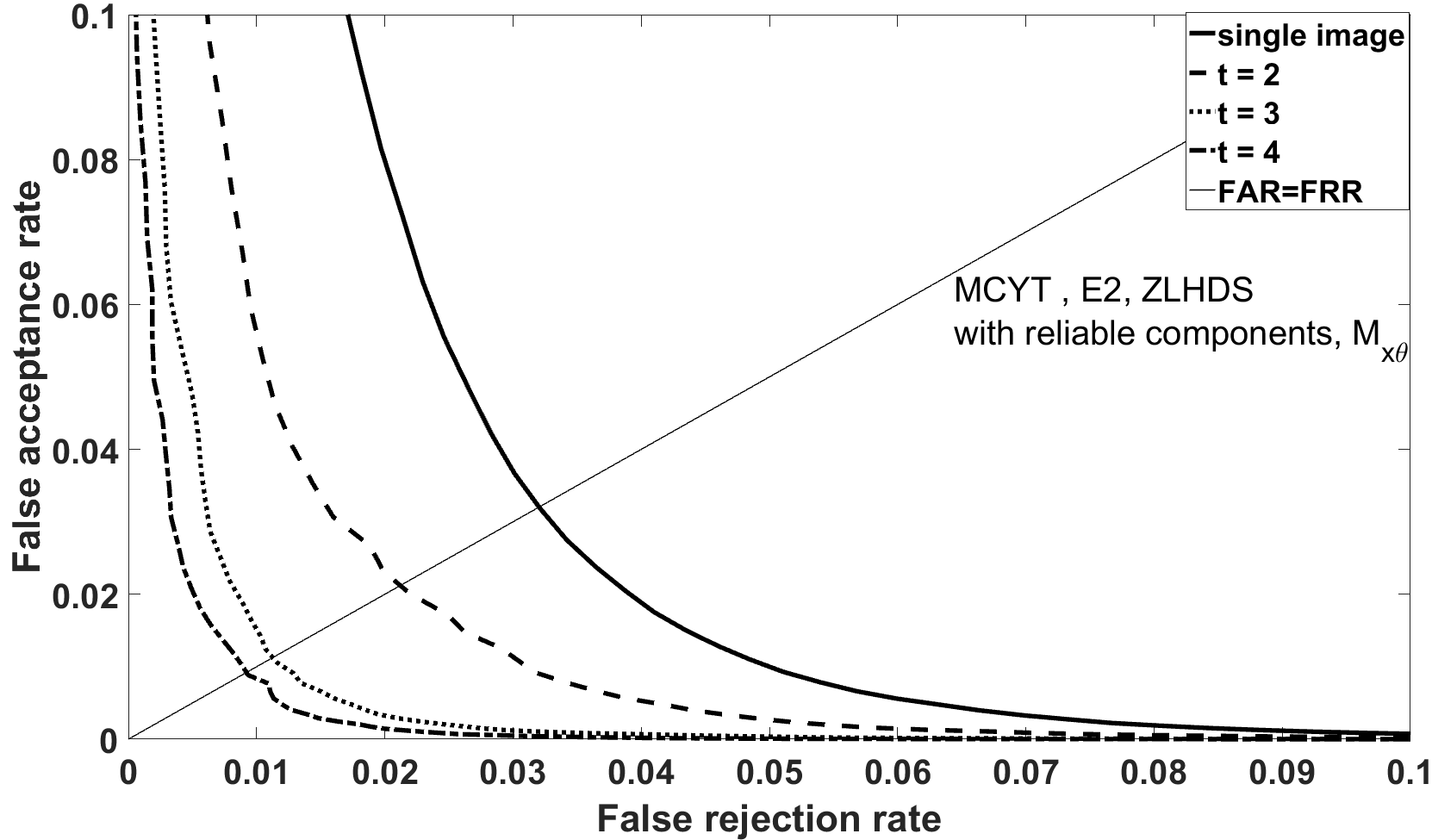
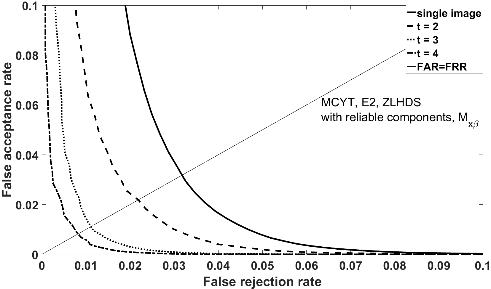
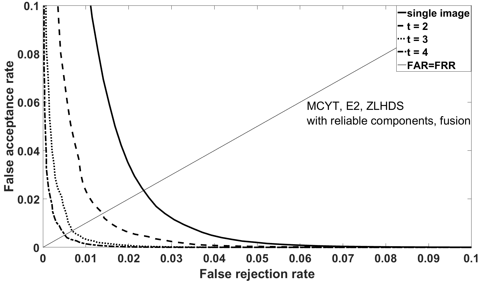
Figure 11: Performance effect of the number of images used for enrollment.

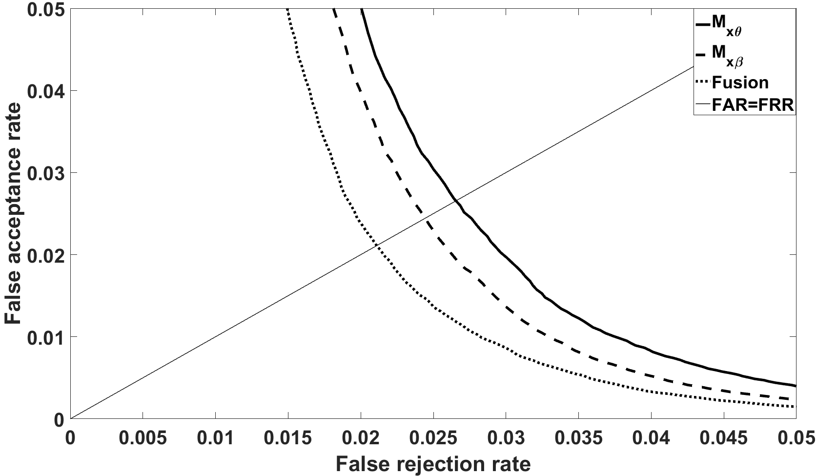
Figure 12: Performance of $M_{x\theta}$ and $M_{x\beta}$ individually, and of their fusion. MCYT database; enrollment method E1; analog domain.

TABLE I: Equal Error Rates and Bit Error Rates. MCYT database. Enrollment methods E1 and E2. Numbers displayed as a percentage are EERs. Numbers without a % sign are BERs: the left number is for genuine pairs, right for impostors.

#images ($t$)		Analog	No HDS		ZLHDS		ZLHDS+r.c.
1	${\cal M}_{x\theta}$	2.6%	3.7%		3.4%		3.2%
			0.33	0.50	0.30	0.49	0.29	0.49
	${\cal M}_{x\beta}$	2.4%	3.7%		3.4%		3.2%
			0.33	0.50	0.31	0.50	0.29	0.49
	Fusion	2.1%	2.9%		2.6%		2.3%
			0.33	0.50	0.30	0.49	0.29	0.49
2	${\cal M}_{x\theta}$	2.1%	3.2%		2.3%		2.1%
			0.33	0.50	0.28	0.46	0.27	0.46
	${\cal M}_{x\beta}$	1.7%	3.01%		2.4%		2.2%
			0.33	0.50	0.28	0.47	0.27	0.47
	Fusion	1.6%	2.3%		1.7%		1.4%
			0.33	0.50	0.28	0.46	0.27	0.47
3	${\cal M}_{x\theta}$	1.4%	2.2%		1.3%		1.1%
			0.31	0.50	0.24	0.45	0.23	0.46
	${\cal M}_{x\beta}$	1.1%	2.0%		1.2%		1.1%
			0.31	0.50	0.25	0.46	0.23	0.46
	Fusion	1.1%	1.5%		0.9%		0.7%
			0.31	0.50	0.24	0.46	0.23	0.46
4	${\cal M}_{x\theta}$	1.2%	1.7%		1.0%		0.9%
			0.29	0.50	0.22	0.45	0.21	0.45
	${\cal M}_{x\beta}$	1.0%	1.6%		0.9%		0.8%
			0.30	0.50	0.22	0.45	0.21	0.45
	Fusion	0.9%	1.1%		0.6%		0.5%
			0.30	0.50	0.22	0.45	0.21	0.45

TABLE II: EERs and BERs for the FVC2000 database. Enrollment methods E1 and E2.

#images ($t$)		Analog	No HDS		ZLHDS		ZLHDS+r.c.
1	${\cal M}_{x\theta}$	6.0%	9.4%		9.0%		8.0%
			0.39	0.50	0.37	0.50	0.36	0.50
	${\cal M}_{x\beta}$	6.1%	10.4%		9.5%		8.1%
			0.39	0.50	0.38	0.50	0.37	0.50
	Fusion	4.8%	7.3%		6.5%		5.5%
			0.39	0.50	0.38	0.50	0.36	0.50
2	${\cal M}_{x\theta}$	4.5%	7.2%		5.7%		5.0%
			0.37	0.50	0.33	0.47	0.32	0.47
	${\cal M}_{x\beta}$	4.8%	7.9%		6.9%		5.6%
			0.38	0.50	0.34	0.47	0.32	0.47
	Fusion	3.9%	5.1%		5.0%		4.1%
			0.37	0.50	0.33	0.47	0.32	0.47
3	${\cal M}_{x\theta}$	3.0%	5.6%		5.3%		4.4%
			0.36	0.50	0.31	0.46	0.29	0.46
	${\cal M}_{x\beta}$	3.2%	7.2%		5.3%		4.9%
			0.37	0.50	0.32	0.46	0.30	0.46
	Fusion	2.2%	4.5%		4.0%		3.3%
			0.37	0.50	0.32	0.46	0.30	0.46
4	${\cal M}_{x\theta}$	2.1%	5.5%		5.5%		4.8%
			0.37	0.50	0.31	0.45	0.29	0.45
	${\cal M}_{x\beta}$	2.2%	7.1%		6.5%		5.0%
			0.37	0.50	0.32	0.46	0.30	0.46
	Fusion	1.3%	4.3%		4.3%		3.3%
			0.37	0.50	0.31	0.45	0.30	0.45

TABLE III: EERs and BERs for the FVC2002 database. Enrollment methods E1 and E2.

#images ($t$)		Analog	No HDS		ZLHDS		ZLHDS+r.c.
1	${\cal M}_{x\theta}$	5.8%	12.1%		10.8%		8.8%
			0.38	0.50	0.37	0.50	0.36	0.50
	${\cal M}_{x\beta}$	6.4%	10.9%		10.9%		9.2%
			0.39	0.50	0.38	0.50	0.36	0.50
	Fusion	5.5%	9.4%		9.3%		7.0%
			0.39	0.50	0.38	0.50	0.36	0.50
2	${\cal M}_{x\theta}$	5.4%	10.9%		9.8%		7.3%
			0.39	0.50	0.35	0.48	0.33	0.48
	${\cal M}_{x\beta}$	5.5%	10.7%		8.4%		7.4%
			0.39	0.50	0.36	0.48	0.34	0.48
	Fusion	4.4%	9.8%		7.3%		5.9%
			0.39	0.50	0.36	0.48	0.34	0.48

TABLE IV: EERs and BERs for the FVC2000 database. Enrollment method E3.

#images ($t$)		Analog	No HDS		ZLHDS		ZLHDS+r.c.
3	${\cal M}_{x\theta}$	3.0%	5.8%		5.2%		4.2%
			0.37	0.50	0.36	0.50	0.34	0.50
	${\cal M}_{x\beta}$	3.2%	8.1%		6.1%		5.4%
			0.37	0.50	0.36	0.50	0.35	0.50
	Fusion	2.2%	5.3%		4.0%		3.1%
			0.37	0.50	0.36	0.50	0.34	0.50

TABLE V: EERs and BERs for the MCYT database. Enrollment method E3.

#images ($t$)		Analog	No HDS		ZLHDS		ZLHDS+r.c.
3	${\cal M}_{x\theta}$	1.4%	2.4%		1.6%		1.4%
			0.31	0.50	0.29	0.49	0.28	0.49
	${\cal M}_{x\beta}$	1.1%	2.2%		1.5%		1.4%
			0.32	0.50	0.30	0.50	0.28	0.50
	Fusion	1.1%	1.6%		1.0%		0.9%
			0.32	0.50	0.30	0.49	0.28	0.50

V-B Error correction: Polar codes

The error rates in the genuine reconstructed $\hat{k}$ are rather high, at least 0.21. In order to apply the Code Offset Method with a decent message size it is necessary to use a code that has a high rate even at small codeword length.

Consider the case of fusion of ${\cal M}_{x\theta}$ and ${\cal M}_{x\beta}$. The codeword length is 1280 bits (1024 if reliable component selection is performed). Suppose we need to distinguish between $2^{20}$ users. Then the message length needs to be at least 20 bits, in spite of the high bit error rate. Furthermore, the security of the template protection is determined by the entropy of the data that is input into the hash function (see Fig. 2); it would be preferable to have at least 64 bits of entropy.

We constructed a number of Polar codes tuned to the signal-to-noise ratios of the individual grid points. The codes are designed to find a set of reliable channels, which are then assigned to the information bits. Each code yields a certain FAR (impostor string accidentally decoding correctly) and FRR (genuine reconstruction string failing to decode correctly), and hence can be represented as a point in an ROC plot. This is shown in Fig. 13. For the MCYT database we have constructed a Polar code with message length 25 at an EER around 1.2% (compared to 0.7% before error correction). For the FVC2000 database we have constructed a Polar code with message length 15 at an EER around 6% (compared to 3.3% EER before error correction). Note that the error correction is an indispensable part of the privacy protection and inevitably leads to a performance penalty. However, we see that the penalty is not that bad, especially for high-quality fingerprints.

From our results we also see that even under the best circumstances (high-quality MCYT database) the entropy of the extracted string is severely limited ($\leq$25 bits). In order to achieve a reasonable security level of the hash, at least two fingers need to be combined. We do not see this as a drawback of our helper data system; given that the EER for one finger is around 1%, which is impractical in real-life applications, it is necessary anyhow to combine multiple fingers.

V-C Error correction: random codebooks

There is a large discrepancy between the message length of the Polar code ($k\leq 25$) and the known information content of a fingerprint. According to Ratha et al [16] the reproducible entropy of a fingerprint image with $Z=35$ robustly detectable minutiae should be more than 120 bits. Furthermore, the potential message size that can be carried in a 1024-bit string with a BER of 23% is $1024[1-h(0.23)]=227$ bits. (And 122 bits at 30% BER.)

We experimented with random codebooks to see if we could extract more entropy from the data than with polar codes. At low code rates, a code based on random codewords can be practical to implement. Let the message size be $\ell$, and the codeword size $m$. A random table needs to be stored of size $2^{\ell}\cdot m$ bits, and the process of decoding consists of computing $2^{\ell}$ Hamming distances. We split the 1024 reliable bits into 4 groups of $m=256$ bits, for which we generated random codebooks, for various values of $\ell$. The total message size is $k=4\ell$ and the total codeword size is $n=4m$. The results are shown in Fig. 13. In short: random codebooks give hardly any improvement over Polar codes.

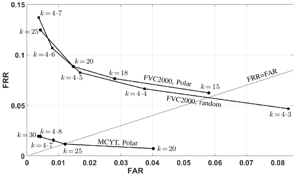
Figure 13: FRR versus FAR achieved by Polar codes and random codebooks (average over three random codebooks). The $\blacklozenge$ markers denote random codebook, and happen to coincide with the line connecting the Polar markers.

VI Summary and discussion

A Helper Data System protects privacy but causes a fingerprint recognition degradation in the form of increased EER. We have built a HDS from a spectral function representation of fingerprint data, combined with a Zero Leakage quantisation scheme. It turns out that our HDS causes only a very small EER penalty when the fingerprint quality is high.

The best results were obtained with the ‘superfinger’ enrollment method (E2, taking the average over multiple enrollment images in the spectral function domain), and with fusion of the ${\cal M}_{x\theta}$,${\cal M}_{x\beta}$ functions. The superfinger method performs slightly better than the E3 method and also has the advantage that it is not restricted to an odd number of enrollment captures.

For the high-quality MCYT database, our HDS achieves an EER around 1% and extracts a 1024-bit string with $\leq 25$ bits of entropy. In practice multiple fingers need to be used in order to obtain an acceptable EER. This automatically increases the entropy of the hashed data. The entropy can be further increased by employing tricks like the Spammed Code Offset Method [19].

As topics for future work we mention (i) testing the HDS on more databases; (ii) further optimisation of parameter choices such as the number of reliable components, and the number of minutiae used in the computation of the spectral functions; (iii) further tweaking of the Polar codes.

References

- [1] VeriFinger SDK. Available online, www.neurotechnology.com.
- [2] E. Arıkan. Channel polarization: a method for constructing capacity-achieving codes for symmetric binary-input memoryless channels. IEEE Transactions on Information Theory, 55(7):3051–3073, 2009.
- [3] R. Canetti, B. Fuller, O. Paneth, L. Reyzin, and A. Smith. Reusable fuzzy extractors for low-entropy distributions. In Eurocrypt 2016, 2016.
- [4] T.M. Cover and J.A. Thomas. Elements of Information Theory. John Wiley & Sons, Inc., Berlin, 2005.
- [5] J. de Groot, B. Škorić, N. de Vreede, and J.P. Linnartz. Quantization in Zero Leakage Helper Data Schemes. EURASIP Journal on Advances in Signal Processing, 2016. 2016:54.
- [6] Y. Dodis, R. Ostrovsky, L. Reyzin, and A. Smith. Fuzzy Extractors: how to generate strong keys from biometrics and other noisy data. SIAM J. Comput., 38(1):97–139, 2008.
- [7] F. Farooq, R.M. Bolle, T.-Y. Jea, and N. Ratha. Anonymous and revocable fingerprint recognition. In IEEE Conference on Computer Vision and Pattern Recognition, pages 1–7. IEEE, 2007.
- [8] D. Frumkin, A. Wasserstrom, A. Davidson, and A. Grafit. Authentication of forensic DNA samples. FSI Genetics, 4(2):95–103, 2010.
- [9] Z. Jin, A.B.J. Teoh, T.S. Ong, and C. Tee. Generating revocable fingerprint template using minutiae pair representation. In International Conference on Education Technology and Computer, pages 251–255. IEEE, 2010.
- [10] A. Juels and M. Wattenberg. A fuzzy commitment scheme. In ACM Conference on Computer and Communications Security (CCS) 1999, pages 28–36, 1999.
- [11] J.-P. Linnartz and P. Tuyls. New shielding functions to enhance privacy and prevent misuse of biometric templates. In Audio- and Video-Based Biometric Person Authentication. Springer, 2003.
- [12] D. Malton, D. Maio, A.K. Jain, and S. Prabhakar. Handbook of Fingerprint Recognition. Springer, London, 2 edition, 2009.
- [13] T. Matsumoto, H. Matsumoto, K. Yamada, and S. Hoshino. Impact of artificial “gummy” fingers on fingerprint systems. In Proc. SPIE, Optical Security and Counterfeit Deterrence Techniques IV, volume 4677, pages 275–289, 2002.
- [14] K. Nandakumar. A fingerprint cryptosystem based on minutiae phase spectrum. In Workshop on Information Forensics and Security (WIFS), pages 1–6. IEEE, 2010.
- [15] J. Ortega-Garcia, J. Fierrez-Aguilar, D. Simon, J. Gonzalez, M. Faundez, V. Espinosa, A. Satue, I. Hernaez, J.J. Igarza, C. Vivaracho, D. Escudero, and Q.I. Moro. MCYT baseline corpus: A bimodal biometric database. In Vision, Image and Signal Processing, Special Issue on Biometrics on the Internet, volume 150, pages 395–401. IEEE, 2003.
- [16] N.K. Ratha, J.H. Connell, and R.M. Bolle. Enhancing security and privacy in biometrics-based authentication systems. IBM Systems Journal, 40:614–634, 2001.
- [17] T. Stanko, F.N. Andini, and B. Škorić. Optimized quantization in Zero Leakage Helper Data Systems. IEEE Transactions on Information Forensics and Security, 12(8):1957–1966, 2017.
- [18] T. Stanko and B. Škorić. Minutia-pair spectral representations for fingerprint template protection. In WIFS 2017. arxiv.org/abs/1703.06811.
- [19] B. Škorić and N. de Vreede. The Spammed Code Offset Method. IEEE Transactions on Information Forensics and Security, 9(5):875–884, 2014.
- [20] C.I. Watson, M.D. Garris, E. Tabassi, C.L. Wilson, R.M. McCabe, S. Janet, and K. Ko. User’s guide to export controlled distribution of NIST biometric image software, 2004. NISTIR 7391.
- [21] H. Xu and R.N.J. Veldhuis. Spectral minutiae representations of fingerprints enhanced by quality data. In Int. Conf. on Biometrics: Theory, Applications and Systems (BTAS) 2009. IEEE, 2009.
- [22] H. Xu and R.N.J. Veldhuis. Spectral representations of fingerprint minutiae subsets. In Image and Signal Processing (CISP) 2009, pages 1–5, 2009.
- [23] H. Xu and R.N.J. Veldhuis. Complex spectral minutiae representation for fingerprint recognition. In Computer Vision and Pattern Recognition Workshop. IEEE, 2010.
- [24] H. Xu, R.N.J. Veldhuis, A.M. Bazen, T.A.M. Kevenaar, A.H.M. Akkermans, and B. Gokberk. Fingerprint verification using spectral minutiae representations. IEEE Transactions on Information Forensics and Security, 4(3):397–409, 2009.