Functional Summaries of Persistence Diagrams

Abstract

One of the primary areas of interest in applied algebraic topology is persistent homology, and, more specifically, the persistence diagram. Persistence diagrams have also become objects of interest in topological data analysis. However, persistence diagrams do not naturally lend themselves to statistical goals, such as inferring certain population characteristics, because their complicated structure makes common algebraic operations–such as addition, division, and multiplication– challenging (e.g., the mean might not be unique). To bypass these issues, several functional summaries of persistence diagrams have been proposed in the literature (e.g. landscape and silhouette functions). The problem of analyzing a set of persistence diagrams then becomes the problem of analyzing a set of functions, which is a topic that has been studied for decades in statistics. First, we review the various functional summaries in the literature and propose a unified framework for the functional summaries. Then, we generalize the definition of persistence landscape functions, establish several theoretical properties of the persistence functional summaries, and demonstrate and discuss their performance in the context of classification using simulated prostate cancer histology data, and two-sample hypothesis tests comparing human and monkey fibrin images, after developing a simulation study using a new data generator we call the Pickup Sticks Simulator (STIX).

1 Introduction

Topological data analysis (TDA) seeks to understand and characterize topological features of data. In particular, persistent homology provides a framework for analyzing the topological connectivity of a dataset at different scales. Persistent homology has drawn interest in applied mathematics (Edelsbrunner et al. 2002, Scopiagno & Zorin 2004, Zomorodian 2005, Ghrist 2008, Carlsson 2009), computer science and machine learning (Adams et al. 2017), statistics (Worsley 1996, Adler et al. 2010, Chazal et al. 2014, Fasy et al. 2014, Turner, Mukherjee & Boyer 2014, Bubenik 2015, Chen et al. 2015), and the applied sciences (Sousbie et al. 2011, Van de Weygaert et al. 2011, Cisewski et al. 2014, Singh et al. 2014, Bendich et al. 2016). The interest in persistent homology is due, at least in part, to its ability to extract summaries of data that are otherwise missed by traditional data analysis methods. Persistent homology gives a multi-scaled way to view data. Different features (in particular, the homology generators) are tracked across the scales, resulting in an object known as the persistence diagram, which is a multi-set of birth-death pairs (indicating the birth and death of the homology generators). While persistence diagrams contain potentially useful information about a dataset, they are not easy objects to use directly in machine learning and statistical settings, so work has been carried out to transform persistence diagrams into one- or two-dimensional functional summaries and vectorized representations. In this article, we review functional summaries of persistence diagrams, develop a unified framework for the functional summaries along with proposing a generalization of a popular functional summary (persistence landscape functions), discuss various ways the functional summaries can be used, and compare the results on simulated and real datasets. Below, we introduce two examples that will be considered in subsequent sections.

Example: Prostate Cancer Histology.

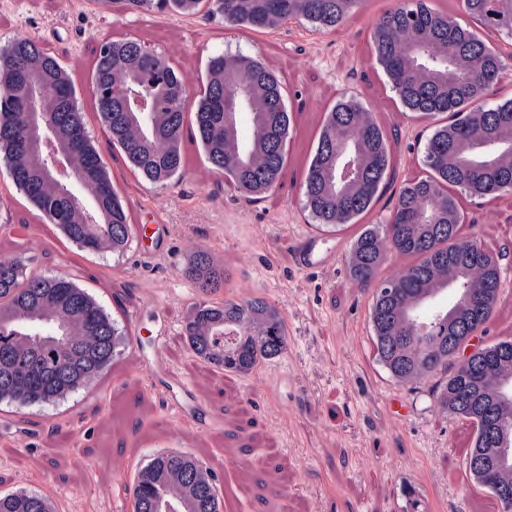
(a) Gleason Grade 3

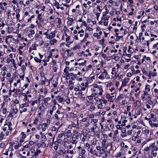
(b) Gleason Grade 5

Figure 1: Sample ROIs from regions graded Gleason Grade $3$ (left) and Gleason Grade $5$ (right). The dark purple are nuclei, and can easily be segmented using software such as CellProfiler(Lamprecht et al. 2007). In the lower-Gleason grades, the nuclei form round circles surrounding glands. As the cancer progresses, these circles become irregular in shape and eventually break open, losing all structure.

Prostate cancer (PCa) is the second most common cancer in men worldwide with an estimated 1.1 million cases diagnosed in 2012 (Center et al. 2012, Ferlay et al. 2015). Prostate cancer diagnosis involves histological classification of hematoxylin and eosin (H&E) prepared slides of a prostate biopsy, such as the region of interest (ROI) from a slide scan shown in Fig. 1. Slides are classified into five grades based on glandular architectural features in the Gleason Grading System; a primary and a secondary grade are assigned, with higher grades corresponding to increasingly poor prognostic outcomes (Humphrey 2004). Initially developed in the 1960s, the Gleason grading system and its recently introduced refinement, the Grade Groups (Epstein et al. 2016), are the most powerful predictors of prognostic outcome in prostate cancer. However, the system suffers from high intra- and inter-observer variability due to the subjective nature of the grading scheme (Engers 2007, Truesdale et al. 2011, Abdollahi et al. 2012, Goodman et al. 2012, Helpap et al. 2012, Truong et al. 2013, Evans et al. 2016). The Gleason grading system and Grade Groups both rely exclusively on architectural patterns of carcinoma cells for histological classification; these architectural patterns provide an opportunity to use topological data analysis. Through a simulation study (Section 5.1), we present a technique for classification of histology slides based on functional summaries of persistence diagrams so that prevalent patterns can be revealed in order to assist a pathologist or oncologist in finding glandular architectural patterns that can be used to assign a Gleason Score or Grade Group.

Example: Fibrin Network Data.

Complicated spatial structures are common in biological data (e.g., fibrin clots, fibroblasts), but are difficult to quantitatively analyze without losing important information. In particular, the coagulation cascade culminates in the web-like structure of a fibrin network. Fig. 2 displays a sample of a human fibrin network collected using a scanning electron microscope; the image are from Pretorius et al. (2009). Features of these structures have numerous implications for vascular diseases like hemophilia and thrombosis (Campbell et al. 2009, Pretorius et al. 2009).

Figure 2: Sample of human fibrin network from Figure 1a of Pretorius et al. (2009), where the white scale bar is 1 $\mu$m.

One of the primary goals of Pretorius et al. (2009) was to compare platelet and fibrin networks of humans and eight other animal species, and carry out an inference procedure to determine if the differences are statistically significant. They focused their comparisons on the thickness of the fibrin fibers and grouped them into thin, intermediate, and thick fibers, requiring measurements of individual fibers within the collection of fibrin networks. To measure the fibers, they randomly selected 100 fibers within the sampled and imaged fibrin networks, and then measured the diameters of the fibers. Next, they assigned the 100 fibers from each fibrin network into one of the three clusters based on the measured diameter, and then did comparisons between the fiber classes of the different species. While they focused on fiber thickness, we compare the topological structure of the fibrin networks using functional summaries of persistence diagrams. In Section 5.2.1, we develop a data-generating model that mimics some of the characteristics of these spatially complex data, including allowing for varying thicknesses of the strands, which we call the Pickup Sticks Simulator (STIX). Before carrying out the hypothesis tests on the real fibrin data, we run a simulation study on the STIX data where we know the ground truth and can verify the methodology.

Additional Applications.

Though we focus on classification and hypothesis tests for prostate cancer histology slides and fibrin networks, the methods we propose can have analogous use in other areas of science. For example, the complicated spatial structure of fibrin networks is similar to the distribution of matter in the Universe, often referred to as the Cosmic Web (Worsley 1996, Sousbie et al. 2011, Van de Weygaert et al. 2011, Wu et al. 2018), and to brain artery trees (Bendich et al. 2016, Biscio & Møller 2016).

Main Contributions.

First, a review is provided of the functional summaries from the literature. Then, we propose a unified framework for the functional summaries and generalize the definition of one popular type of persistence functional summary, the persistence landscape function, to a broader class of functions that allows for different kernels and bandwidths providing additional flexibility for the practitioner. Theoretical properties of the persistence functional summaries are established, putting these functional summaries on a solid foundation for various types of statistical inference and methodology. Then, several of the popular functional summaries, along with the proposed generalized landscape function, are used in two different applications in order to compare their performance. The first is using simulated prostate cancer histology data, where the data are classified according to simulated architectural morphology. The second application carries out two-sample hypothesis tests comparing human and monkey fibrin images, which is particularly challenging because the data have a complicated, web-like, spatial structure. In order to evaluate the performance in a more controlled setting, we develop a new data-generating mechanism, STIX. STIX generates images that have similar features to the fibrin data, but are also interesting objects of study on their own.

2 Functional Summaries of Persistence Diagrams

Before introducing functional summaries of persistence diagrams, we provide an introduction to persistence diagrams themselves, along with some examples of the types of inference one may want to do with a set, or sets, of persistence diagrams.

2.1 Persistence Diagrams

In TDA, persistence diagrams (Cohen-Steiner et al. 2007, Edelsbrunner & Morozov 2012, Wasserman 2016) provide a useful way to summarize the topological structure of a point-cloud of data or a function. In this introduction, we focus on the function-based filtrations for persistence diagrams, but other types of filtrations can be used. For more details on filtrations over point clouds, we suggest Zhu (2013) or Ghrist (2014). Given a function $f:\mathcal{X}\to\mbox{$\mathbb{R}$}$, where $\mathcal{X}$ is a topological space, we define the upper $\lambda$-level set of $f$ as

$$L_{\lambda}=\{x:f(x)\geq\lambda\}=f^{-1}([\lambda,\infty)).$$

For any two level thresholds $\lambda_{1}>\lambda_{2}$, the corresponding level sets satisfy $L_{\lambda_{1}}\subset L_{\lambda_{2}}$. Thus, the collection of level sets $\mathcal{L}=\bigcup_{\lambda}\{L_{\lambda}\}$ forms a filtration with the level as the index set.

For each level set $L_{\lambda}$, its topological features are captured through the generators of its homology groups. Informally, the $0$-th order homology groups ($0$-th order topological feature) capture the connected components, the $1$-st order homology groups capture regions forming a loop structure, and $2$-nd order homology groups capture regions forming a void structure. For the formal definition of homology groups, we refer readers to Edelsbrunner & Harer (2008) and Edelsbrunner & Morozov (2012). When we decrease the level $\lambda$, new generators for the homology groups may be created (e.g., the formation of new components), existing generators may merge together (e.g., two connected components joining together), and existing generators may be eliminated (e.g., a loop getting filled in). The level at which a generator is created is called its birth time and the level at which a generator is eliminated, or merges with another generator that has an earlier birth time, is called its death time. Thus, for every generator in $\mathcal{L}$, there are three characteristics: homology order, birth time, and death time.

The persistence diagram is the collection of all these triplets of the filtration formed by the given function $f$. Thus, if a function’s filtration has $|D|$ generators, then its persistence diagram is

$$\mbox{$\sf D$}=\{(r_{j},b_{j},d_{j}):j=1,\cdots,|D|\},$$

where $r_{j},b_{j},$ and $d_{j}$ are the homology order, birth time, and death time of the $j$-th generator, respectively, and the norm $|D|$ denotes the number of off-diagonal elements in the persistence diagram $\sf D$.

2.1.1 Example: constructing a persistence diagram from a dataset

There are many ways of constructing a persistence diagram from a dataset. If the data are images, functions, or fields evaluated on a grid, then the construction of the corresponding persistence diagrams is straight forward – we just consider the pixels, or grid points, whose value is above a given level and vary such level to construct a filtration.

When the data are a collection of points, the construction of a persistence diagram depends on how the function that generates the underlying filtration is constructed. Here we illustrate the construction using an estimator of the underlying density function. We use a kernel density estimate (KDE) to estimate the underlying probability density function that generates this data and construct the filtration using the (upper) level set of the KDE (Fasy et al. 2014, Wasserman 2016). This procedure is summarized in Fig. 3, where we obtain a persistence diagram for the estimated density function of the given 2D point clouds. Formally, let $X_{1},\cdots,X_{n}\in\mbox{$\mathbb{R}$}^{d}$ be the observed values for a single dataset. The KDE is $\widehat{p}_{h}(x)=\frac{1}{nh^{d}}\sum_{i=1}^{n}K\left(\frac{\|X_{i}-x\|}{h}\right),$ where $K(x)$ is a smooth function called the kernel function (e.g. a Gaussian kernel) and $h>0$ is a quantity called the smoothing bandwidth that controls the amount of smoothing (Wasserman 2006). Using $\widehat{p}_{h}$ and its level sets, we then construct the persistence diagram which contains topological information about the underlying density function.

(a) Dataset

(b) KDE

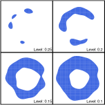
(c) Level Set

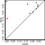
(d) PD

Figure 3: The construction of a persistence diagram from the single dataset (points) displayed in (a). We construct the persistence diagram (PD, d) using level sets (e.g., c) of its kernel density estimator (b).

2.2 Modeling multiple persistence diagrams

In this paper, we focus on the case where multiple persistence diagrams, $\mbox{$\sf D$}_{1},\dots,\mbox{$\sf D$}_{n},$ are observed and we want to perform statistical analysis (e.g., estimating population quantities, classification, hypothesis testing) over these diagrams. In addition to the prostate cancer histology data and fibrin network data mentioned previously, there are many other situations where this framework is useful, such as when analyzing brain artery trees (Bendich et al. 2016, Biscio & Møller 2016), investigating the large-scale structure of the Universe using cosmological simulations (Wu et al. 2018), or studying shape data (Turner, Mukherjee & Boyer 2014, Crawford et al. 2016). A common assumption in these examples is that the persistence diagrams, $\mbox{$\sf D$}_{1},\dots,\mbox{$\sf D$}_{n}$, are generated from the same population. Thus, we can model this procedure as the case where there exists a distribution of persistence diagrams $\mathcal{P}$ (Mileyko et al. 2011) such that $\mbox{$\sf D$}_{1},\dots,\mbox{$\sf D$}_{n}$ are independent and identically distributed from $\mathcal{P}$.

Unfortunately, persistence diagrams are not easy objects to work with. Even if a sample of persistence diagrams are from the same distribution, each of them may have different numbers of topological features, and those features have a complicated covariance. This makes it difficult to carry out common algebraic operations such as addition, division, and multiplication, hence computing statistical summaries such as means and medians is challenging (Turner 2013, Turner, Mileyko, Mukherjee & Harer 2014). In the multiple diagram setting, a simple but elegant approach is to summarize each diagram by a function and then analyze the diagrams by comparing their corresponding functions. Because functions are well-defined objects, and statistical analysis over functions are well-studied, analyzing these functional summaries is a much easier task than directly studying the diagrams.

The proposed functional summaries use either a univariate or a bivariate function function to summarize the persistence diagram, but, in general, functions with more variables can be used. A brief review of the existing functional summaries of persistence diagrams is provided next, before giving more details on the proposed functional summaries. Let $\cal F$ be a collection of functions. Then, a functional summary of a persistence diagram, $\mathbb{F}(\mbox{$\sf D$})$, is a map between $\cal D$ and $\cal F$. i.e.,

$$\mathbb{F}:\mbox{$\cal D$}\to\mbox{$\cal F$}.$$

Using a functional summary $\mathbb{F}$, the random diagrams $\mbox{$\sf D$}_{1},\cdots,\mbox{$\sf D$}_{n}$ become random functions $F_{1}=\mathbb{F}(\mbox{$\sf D$}_{1}),\cdots,F_{n}=\mathbb{F}(\mbox{$\sf D$}_{n})$. Moreover, since these random diagrams are from the same distribution, the corresponding functional summaries also come from the same distribution (of functions), $\mathcal{P}_{F}$:

$$F_{1},\cdots,F_{n}\overset{i.i.d.}{\sim}\mathcal{P}_{F}.$$ (1)

The above characterizes the statistical model for using functional summaries to analyze persistence diagrams. Except where noted, we focus on topological features of the same homological dimension.

2.3 Review: Functional Summaries

We review several functional summaries that have been proposed in existing literature.

2.3.1 Persistence Landscape

The persistence landscape function is a popular univariate functional summary of a persistence diagram (Chazal et al. 2014, Bubenik 2015). To produce a persistence landscape function, or simply referred to as a landscape function, the persistence diagram is rotated clockwise 45 degrees, and then isosceles right triangles are drawn from each feature of a particular homology dimension (where the right angle vertex is the homology feature). From the collection of isosceles right triangles, individual functions are traced out where the first landscape function is the point-wise maximum of all the triangles drawn. More specifically, a persistence landscape is a collection of univariate functional summaries $\mathbb{F}_{k}:\mbox{$\cal D$}\to\mbox{$\cal F$}$ such that for each $k\in\mbox{$\mathbb{N}$}$,

$$\mathbb{F}_{k}(\mbox{$\sf D$};t)=\underset{j=1,\cdots,|\mbox{$\sf D$}|}{\sf kmax}\{\Lambda_{j}(t)\},$$ (2)

where $\Lambda_{j}(t)=\min(t-b_{j},d_{j}-t)_{+}$, ${\sf kmax}$ is a function selecting the $k$-th largest value, and the norm $|\mbox{$\sf D$}|$ denotes the number of off-diagonal elements in the persistence diagram $\sf D$. An illustration of this is displayed in Fig. 4.

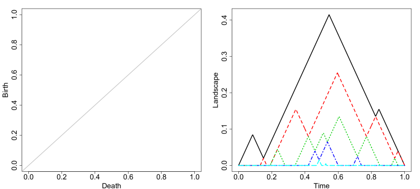
Figure 4: Illustration of a persistence landscape function. The left plot is a persistence diagram and the right plot is its corresponding persistence landscape function; each color and line style represents a different $\mathbb{F}_{k}$ with $\mathbb{F}_{1}$ as the solid black line, $\mathbb{F}_{2}$ as the dashed red line, etc.

2.3.2 Persistence Silhouette

Persistence silhouette functions were introduced in Chazal et al. (2014) as a modification of the persistence landscape function. The persistence silhouette function maps the persistence diagram to a function $\mbox{$\cal D$}\to\mbox{$\mathbb{R}$}$, as opposed to $\mbox{$\cal D$}\to\mbox{$\mathbb{R}$}\times\mbox{$\mathbb{N}$}$ with landscape functions, by combining all the layers of the landscapes functions into a single, average function. The persistence silhouette is a function $\mathbb{F}:\mbox{$\cal D$}\to\mbox{$\cal F$}_{1}$ such that

$$\mathbb{F}(\mbox{$\sf D$};t)=\frac{\sum_{j=1}^{\left|\mbox{$\sf D$}\right|}\omega(d_{j}-b_{j})\Lambda_{j}(t)}{\sum_{k=1}^{\left|\mbox{$\sf D$}\right|}\omega(d_{k}-b_{k})},$$

where $\omega(d_{j}-b_{j})$ is a weight function based on the persistence of the features. For example, the weight function $\omega(d_{j}-b_{j})=|d_{j}-b_{j}|^{p}$ could be used, where $p$ is a tuning parameter that has to be selected. Larger values of $p$ put more weight on the features with longer lifetimes, and smaller values of $p$ emphasize the features with shorter lifetimes.

2.3.3 Accumulative Persistence Function

The accumulative persistence function (APF), introduced in Biscio & Møller (2016), is a univariate functional summaries $\mathbb{F}:\mbox{$\cal D$}\to\mbox{$\cal F$}_{1}$ such that

$$\mathbb{F}(\mbox{$\sf D$};t)=\sum_{j=1}^{\left|\mbox{$\sf D$}\right|}(d_{j}-b_{j})\cdot I(d_{j}+b_{j}\leq 2t).$$

The APF behaves like a cumulative distribution function in that it is a non-decreasing function.

2.3.4 Persistence Intensity and Image

The persistence intensity is a bivariate functional summary (Chen et al. 2015), where $\mathbb{F}:\mbox{$\cal D$}\to\mbox{$\cal F$}_{2}$ is a map to a bivariate function defined as

$$\mathbb{F}(\mbox{$\sf D$};t,s)= \frac{1}{\left|\mbox{$\sf D$}\right|}\sum_{j=1}^{\left|\mbox{$\sf D$}\right|}\omega(d_{j}-b_{j})\cdot K\left(\frac{\sqrt{|b_{j}-t|^{2}+|d_{j}-s|^{2}}}{h}\right),$$ (3)

where $\omega$ is a weight function and $K$ is a kernel function with smoothing parameter $h$. The persistence intensity replaces points on the persistence diagrams by a smooth localized function that is determined by the kernel function $L$ (the amount of smoothing is determined by the parameter $h$) and apply a weighted sum over all points to form an intensity function such that, for example, points far away from the diagonal (features that are more persistent) are given higher weights. This leads to a bivariate function that summarizes a persistence diagram.

Note that if we evaluate the bivariate functional summary on a grid and view it as an image, we obtain the persistence image introduced in Adams et al. (2017). The persistence image framework of Adams et al. (2017) includes vectorizing the image making it suitable for many machine learning and statistical methods.

Remark 1

When we can have an extra scale parameter for each persistence diagram, we can construct a special bivariate functional summary called the persistence flamelet. The persistence flamelet (Padellini & Brutti 2017) is a bivariate functional summary that combines the persistence landscape and the scale parameter. For instance, the persistence diagram may be constructed from a KDE of a point could making the smoothing bandwidth $h$ in the KDE the scale parameter. In this case, the persistence landscape also depends on the scale parameter $h$. The persistence flamelet is a bivariate function of $(t,h)$ such that for each fixed $h$, the persistence flamelet is the persistence landscape.

Remark 2

In addition to functional summaries of persistence diagrams, one might want vector-valued summaries for input to machine learning algorithms, for instance. In Adcock et al. (2016), the authors define an algebra of functions on the space of persistence bar codes. Furthermore, they identify the generators of this algebra, and show the utility of these functions through applications of classification of data using machine learning. In addition, using the maximum persistence alone has proven successful in certain settings (Khasawneh & Munch 2014, Perea & Harer 2015).

3 Generalized Landscape Functions

As noted previously, landscape functions result from a persistence diagram that is rotated, and then each feature $j$ on the diagram produces an isosceles right triangle, $\Lambda_{j}$. However, one need not be restricted to these special triangles when computing one-dimensional functional summaries of persistence diagrams. We propose an expanded class of persistence landscape functions, called generalized persistence landscape functions. With these generalized landscapes, one can substitute different kernels (e.g. tricube, Epanechnikov) and different bandwidths in order to better adapt to the details in the persistence diagram. (See Wasserman (2006) for a general discussion about kernel functions and bandwidth selection.) The triangle kernel used in the original landscape function definition can also be used, except the width of the base of the triangle can be adjusted, which could be analogously thought of as adjusting the angles of the triangle.

More specifically, the change is in the form of $\Lambda_{j}$ from Equation (2), where the generalized landscapes use

$$\widetilde{\Lambda}_{j}(t;h)=\begin{cases}\frac{y_{j}}{K_{h}(0)}K_{h}\left({t-x_{j}}\right),&\text{for }|\frac{t-x_{j}}{h}|\leq 1\\ 0,&\text{otherwise, }\end{cases}$$

where $K_{h}$ is the kernel function with $h$ as the bandwidth, $(x_{j},y_{j})$ is the rotated feature corresponding to $(b_{j},d_{j})$ from the persistence diagram, with $x_{j}=(b_{j}+d_{j})/2$ and $y_{j}=(d_{j}-b_{j})/2$, and the $\frac{y_{j}}{K_{h}(0)}$ ensures that $\widetilde{\Lambda}_{j}$ goes through $(x_{j},y_{j})$. For example, the Epanechnikov kernel would have $\widetilde{\Lambda}_{j}(t;h)=(y_{j})(1-|\frac{t-x_{j}}{h}|^{2})$ for $|\frac{t-x_{j}}{h}|\leq 1$. Using the new definitions of $\widetilde{\Lambda}_{j}$, the generalized landscapes are defined in the same manner as landscapes:

$$\widetilde{\mathbb{F}}_{k}(\mbox{$\sf D$};t)=\underset{j=1,\cdots,|\mbox{$\sf D$}|}{\sf kmax}\{\widetilde{\Lambda}_{j}(t;h)\},.$$ (4)

Illustrations of several generalized landscape functions are displayed in Fig. 5 using the triangle kernel. As with general nonparametric smoothing methods, a smaller bandwidth results in a rougher function and a larger bandwidth results in a smoother function. In Sections 5.1 and 5.2, we consider both generalized landscapes and original landscapes in a classification problem and in two sample hypothesis tests. Although the generalized landscapes and the landscape functions ultimately contain the same information, a benefit of using the generalized landscapes is that more features of the persistence diagram can be isolated to fewer function layers.

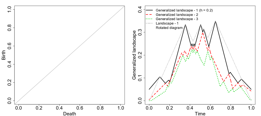
Figure 5: Generalized persistence landscape functions. The left plot is the persistence diagram used to produce the functional summaries in the right plot. In the right plot, the black circles are the rotated persistence diagram features, the solid black line is the first generalized landscape using the triangle kernel with a bandwidth (half the triangle base) of $h=0.2$, the second and third generalized landscapes are plotted in red dashes and green dots, respectively. As a comparison, the first landscape function is plotted in gray as lines and dots.

4 Methodology

All functional summaries defined in the previous section map a persistence diagram to a function. The problem of analyzing random persistence diagrams becomes the problem of analyzing random functions, which is a topic that has been studied for decades in statistics (Van der Vaart 2000). Next, we describe some analysis methods that can be done using the statistical model characterized in (1).

4.1 Population quantities

Using the statistical model of (1), we can define various population quantities associated to the functional summaries such as the mean functional summary (Chazal et al. 2014, Chen et al. 2015, Biscio & Møller 2016). When averaging functional summaries of diagrams, we obtain a sample mean functional summary. This quantity can be used as an estimator of the population mean functional summary. In more detail, the population mean functional summary is a function

$$\bar{F}(t)=\mathbb{E}(F_{i}(t)),$$

where the expectation $\mathbb{E}$ is with respect to the distribution $\mathcal{P}_{F}$. The sample estimator is then the pointwise estimator

$$\widehat{F}(t)=\frac{1}{n}\sum_{i=1}^{n}F_{i}(t),$$

and the convergence of $\widehat{F}$ toward $\bar{F}$ can be studied using notions of convergence of functions (Chazal et al. 2014, Chen et al. 2015).

Let $\mathcal{B}_{F}$ be the set of all possible functions formed by a given functional summary, and let $\mathbb{T}$ be a compact set such that we are interested in the population mean functional summary $\bar{F}(t)$ within $t\in\mathbb{T}$. To simplify the problem, we define $F(t)=0$ for all $t\notin\mathbb{T}$ for every $F\in\mathcal{B}_{F}$. Throughout the paper, we assume that the functional summary is uniformly bounded by a constant $\bar{U}<\infty$. Namely,

$$\sup_{F\in\mathcal{B}_{F}}\sup_{x\in\mathbb{T}}|F(x)|\leq\bar{U}.$$ (5)

The following is a simple convergence theorem of the estimator $\widehat{F}$, which shows that as long as the functional summary is continuous, the sample mean function summary $\widehat{F}$ uniformly converges to $\bar{F}$ almost surely, as expressed in the following proposition.

Proposition 1 (Pointwise Convergence)

Assume Equation (5) holds. If $\mathcal{B}_{F}$ is equicontinuous, then

$$\sup_{t\in\mathbb{T}}|\widehat{F}(t)-\bar{F}(t)|\overset{a.s.}{\rightarrow}0.$$

As a result, if there exists a constant $L>0$ such that any $F\in\mathcal{B}_{F}$ is $L$-Lipschitz, then

$$\sup_{t\in\mathbb{T}}|\widehat{F}(t)-\bar{F}(t)|\overset{a.s.}{\rightarrow}0.$$

The proof is presented in Appendix B. Persistence intensity, persistence landscapes and generalized landscapes, and persistence scoring all satisfy the condition in Proposition 1 as long as the number of homological features and the lifetime of the features are uniformly bounded. Thus, averaging these functional summaries yields a consistent estimate of the corresponding population mean functional summary.

The difference $\widehat{F}(t)-\bar{F}(t)$ is tightly related to a normal distribution. In what follows, we show that it converges to a normal distribution in various ways. Let $\mathcal{W}=\{\mathbb{F}_{t}:t\in\mathbb{T}\}$ such that $\mathbb{F}_{t}(D_{i})=F_{i}(t)$ for each $i=1,\cdots,n$ be the mapping from the persistence diagram $D_{i}$ to a functional summary as displayed in Equation (1). Let $Q$ be a probability measure over $\mathcal{B}_{F}$ and define $\|f-g\|_{Q,2}=\sqrt{\int|f(t)-g(t)|^{2}dQ(t)}$ be the $L_{2}(Q)$ norm for functions and $N(\mathcal{W},L_{2}(Q),\epsilon)$ be the $\epsilon$-covering number of $\mathcal{W}$.

Proposition 2

Let $\sigma^{2}(t)={\sf Var}(F_{i}(t))$ and $\sigma^{2}=\int\sigma^{2}(t)dt$. Assume Equation (5) holds, then

$$\sqrt{n}\left(\widehat{F}(t)-\bar{F}(t)\right) \overset{D}{\rightarrow}N(0,\sigma^{2}(t))$$

$$\sqrt{n}\int\left(\widehat{F}(t)-\bar{F}(t)\right)dt \overset{D}{\rightarrow}N(0,\sigma^{2}).$$

Moreover, if

$$\int_{0}^{1}\sqrt{\log\sup_{Q}N(\mathcal{W},L_{2}(Q),\epsilon\bar{U})}d\epsilon<\infty,$$ (6)

where $\bar{U}$ is the upper bound of the functional summary and the supremum is taken over all finitely discrete probability measures on the space of persistence diagrams , then $\sqrt{n}\left(\widehat{F}-\bar{F}\right)$ converges in distribution to $\mathbb{B}$, where $\mathbb{B}(t)$ is a Gaussian process over $t\in\mathbb{T}$ with a covariance function

$${\sf Cov}(\mathbb{B}(t),\mathbb{B}(s))=\mathbb{E}(F_{i}(t)F_{i}(s))-\bar{F}(t)\bar{F}(s)$$

for $t,s\in\mathbb{T}$. Futhermore, if there exists a constant $L>0$ such that any $F\in\mathcal{B}_{F}$ is $L$-Lipschitz, then the above three convergences hold.

The proof is presented in Appendix B. Proposition 2 presents the asymptotic normality of the sample mean functional summary. The assumptions are from the Donsker theorem; see, e.g., page 18 of Kosorok (2007). The convergence toward a Gaussian process further implies the convergence of the supremum, i.e.,

$$\sqrt{n}\sup_{t\in\mathbb{T}}|\widehat{F}(t)-\bar{F}(t)|\overset{D}{\rightarrow}\sup_{t\in\mathbb{T}}|\mathbb{B}(t)|,$$

by the continuous mapping theorem; see page 16 of Kosorok (2007) for more detailed discussion.

The assumption (6) is quite mild. If the functional summary is $L$-Lipschitz, then Equation (6) holds and thus $\sqrt{n}\left(\widehat{F}-\bar{F}\right)$ converges to a Gaussian process. A good news is that many functional summaries, such as the persistence landscapes, persistence silhouette, persistence image, and persistence intensity are all $L$-Lipschitz functional summaries under a very mild assumption (the number of features in the persistence diagrams is finite almost surely). For the generalized landscape, as long as the kernel function $K$ is Lipschitz (which is true for most of the common kernel functions), the functional summary is also Lipschitz.

4.2 Confidence Bands

Confidence bands provide a way to assess and visualize the uncertainty in the sample mean functional summary, which can be constructed using a bootstrapping procedure (Chazal et al. 2014). Specifically, given a confidence level $\alpha$, the bootstrap can be employed to find a fixed bandwidth upper envelope function $U_{1-\alpha}(t)$ and a lower envelope function $L_{1-\alpha}(t)$ such that

$$P(L_{1-\alpha}(t)\leq\bar{F}(t)\leq U_{1-\alpha}(t) \,\,\,\forall t\in[a,b])$$

$$=1-\alpha+o(1),$$

for some regions $[a,b]$. See Proposition 3 below for more details.

The following are the details of the construction of a confidence band. Note that we assume the functional summary is a univariate function for simplicity; one can easily generalize the following for multivariate functions.

1. The initial estimate. First, compute the sample mean functional summary, $\widehat{F}(t)=\frac{1}{n}\sum_{i=1}^{n}F_{i}(t),$ for $t\in[a,b]$, a given interval.

2. The bootstrap procedure. Sample diagrams with replacement and compute the corresponding functional summaries and the sample mean functional summary, denoted as $\widehat{F}^{*}(t)$. Namely, generate $\mbox{$\sf D$}^{*}_{1},\cdots,\mbox{$\sf D$}^{*}_{n}$ by sampling randomly (with replacement) from $\mbox{$\sf D$}_{1},\cdots,\mbox{$\sf D$}_{n}$ in a way such that each diagram has an equal probability $(1/n)$ of being selected. Then compute the the corresponding functional summaries $F^{*}_{1},\cdots,F^{*}_{n}$, and calculate the sample mean functional summary, $\widehat{F}^{*}(t)$.

3. Replication. Repeat the bootstrap procedure $B$ times, leading to $B$ bootstrap realizations of the sample mean functional summary, denoted as

   $$\widehat{F}^{*(1)}(t),\cdots,\widehat{F}^{*(B)}(t).$$

4. Width of band. For a given significance level $\alpha$, choose

   $$\widehat{t}_{1-\alpha}=\widehat{G}^{-1}(1-\alpha),\quad\widehat{G}(s)=\frac{1}{B}\sum_{j=1}^{B}I\left(\sup_{t}\|\widehat{F}^{*(j)}(t)-\widehat{F}(t)\|\leq s\right),$$

   where $\widehat{t}_{1-\alpha}$ is the $1-\alpha$ quantile of the $L_{\infty}$-distance between the bootstrap realizations and the initial estimate.

5. Output. The upper and lower bound of the confidence band is

   $$U_{1-\alpha}(t)=\widehat{F}(t)+\widehat{t}_{1-\alpha},\quad L_{1-\alpha}(t)=\widehat{F}(t)-\widehat{t}_{1-\alpha}.$$

The following proposition shows that the confidence band is consistent under mild assumptions.

Proposition 3 (Functional Bands)

If the assumptions in Proposition 2, including Equation (6), hold, then

$$P\large(L_{1-\alpha}(t)\leq\bar{F}(t)\leq U_{1-\alpha}(t)\,\,\forall t\in\mathbb{T}\large)=1-\alpha+o(1).$$

The proof is presented in Appendix B. Proposition 3 shows that the confidence band is asymptotically valid. Note that if a slightly stronger assumption is made,

$$\sup_{Q}N(\mathcal{W},L_{2}(Q),\epsilon\bar{U})\leq A\left(\frac{1}{\epsilon}\right)^{\nu},$$ (7)

for some constants $A,\nu>0$, then we can replace the $o(1)$ in proposition 3 by $O(n^{-1/8})$; see the derivation of Chazal et al. (2014).

The above procedure provides a fixed bandwidth confidence band. A variable-bandwidth confidence band can also be constructed using a simple modification in Step 4 and 5. First, compute a variance estimator of the functional summaries

$$\widehat{\sigma}^{2}(t)=\frac{1}{n}\sum_{i=1}^{n}\left(F_{i}(t)-\widehat{F}(t)\right)^{2}.$$ (8)

Then, in Step 4, choose

$$\widehat{s}^{\dagger}_{1-\alpha}=\widehat{G}_{\dagger}^{-1}(1-\alpha),\quad\widehat{G}_{\dagger}(s)=\frac{1}{B}\sum_{j=1}^{B}I\left(\sup_{t}\left\|\frac{\widehat{F}^{*(j)}(t)-\widehat{F}(t)}{\widehat{\sigma}(t)}\right\|\leq s\right).$$

And, in Step 5, we construct the band via

$$U^{\dagger}_{1-\alpha}(t)=\widehat{F}(t)+\widehat{s}^{\dagger}_{1-\alpha}\cdot\widehat{\sigma}(t),\quad L^{\dagger}_{1-\alpha}(t)=\widehat{F}(t)-\widehat{s}^{\dagger}_{1-\alpha}\cdot\widehat{\sigma}(t).$$

Using a similar derivation as Chazal et al. (2014), one can prove that such a confidence band is also valid

Note that both equations (6) and (7) hold if the functional summaries are $L$-Lipschitz. Therefore, we have the following result for the generalized landscapes.

Corollary 1

Assume that $\mathbb{T}$ is compact and the number of topological features of a persistence diagram is bounded by a constant almost surely. If the functional summaries are constructed by a generalized persistence landscape with a Lipschitz kernel function and a fixed $h>0$, then the conclusions in proposition 1, 2, and 3 are true.

Corollary 1 is a direct result from the three propositions when the kernel function is Lipschitz. Most common kernel functions such as the triangle kernel and the Gaussian kernel satisfy this condition. Thus, this corollary implies that the generalized landscape function is a stable functional summary for data analysis.

4.3 Prediction Bands

A sample mean functional summary $\widehat{F}$ can be used to predict the outcome of a future persistence functional summary. Let $d:\mathcal{F}\times\mathcal{F}\mapsto\mathbb{R}$ be a metric for functional summaries. For every functional summary, say $F_{i}$, we first compute the residual, $e_{i}=d(F_{i},\widehat{F}),$ and then pick $\widehat{q}_{\gamma}$ to be the $\gamma$-quantile of $e_{1},\cdots,e_{n}$. Then a $\gamma$-prediction set is

$$\widehat{\mathcal{F}}_{\gamma}=\{F:d(F,\widehat{F})\leq\widehat{q}_{\gamma}\}.$$ (9)

The following Proposition 4 proves that the prediction set in Equation (9) is a valid prediction set in our setting.

Proposition 4

Let $d$ be a metric for functional summaries such that

$$d(\widehat{F},\bar{F})\overset{P}{\rightarrow}0.$$

Moreover, assume that the function

$$Q(t)=P(d(F_{i},\bar{F})<t)$$

has a finite derivative bounded away from $0$ at an open neighborhood containing $t=q_{\gamma}$, where $q_{\gamma}$ solves $Q(q_{\gamma})=\gamma$. Let $\widehat{\mathcal{F}}_{\gamma}$ be as defined in Equation (9). Then

$$P(F_{\sf new}\subset\widehat{\mathcal{F}}_{\gamma}|F_{1},\cdots,F_{n})=\gamma+O_{P}\left(\left(\frac{1}{\sqrt{n}}\right)+d(\widehat{F},\bar{F})\right).$$

The proof is presented in Appendix B. Note that the assumption $d(\widehat{F},\bar{F})\overset{P}{\rightarrow}0$ is very mild requiring that our estimator is consistent under the metric $d$. The second assumption, the continuity of $Q(t)$ at $t=q_{\gamma}$, is also very weak; if the random variable $d(F_{i},\bar{F})$ has a density function that takes non-zero value around $t=q_{\gamma}$, then this assumption holds. Just as other propositions, Proposition 4 also applies to the generalized landscape when the kernel function is Lipschitz.

There are many possible metrics $d$, and common choices are

$$d_{p,\omega}(F,G) =\left(\int\left(\frac{|F(t)-G(t)|}{\omega(t)}\right)^{p}dt\right)^{\frac{1}{p}}$$ (10)

$$d_{\infty,\omega}(F,G) =\sup_{t}\left|\frac{F(t)-G(t)}{\omega(t)}\right|$$

where $\omega(t)>0$ is a weight function and $p$ is a positive number. When $\omega(t)=1$, $d_{p,\omega}$ becomes the $L_{p}$-metric for functions and we often write $d_{p}=d_{p,\omega}$ for simplicity. $d_{1}$ and $d_{2}$ are popular choice in data analysis. However, the prediction set $\widehat{\mathcal{F}}_{\gamma}$ from $d_{1}$ or $d_{2}$ (or any other $d_{q}$ for $0<q<\infty$) is hard to visualize. The $L_{\infty}$ metric $d_{\infty}$ leads to a prediction set that is easy to visualize, but $d_{\infty}$ can be too sensitive to small perturbations.

To obtain a stable metric with a simple visualization property, we consider the metric $d_{\infty,\omega}$ with $\omega(t)=\widehat{\sigma}(t)=\sqrt{\widehat{\sigma}^{2}(t)}$, the estimated standard deviation of $F_{1}(t),\ldots,F_{n}(t)$ from Equation (8). This leads to a variable-width prediction band. The prediction band can be constructed by first computing $e_{i}=d_{\infty,\widehat{\sigma}}(F_{i},\widehat{F})$ for each $i=1,\cdots,n$. Given a prediction level $\gamma>0$, let

$$\widehat{q}_{\gamma}=\gamma\mbox{-quantile of }\{e_{1},\cdots,e_{n}\}.$$

Then the $\gamma$-prediction band is

$$\left\{f(t):\widetilde{L}_{\gamma}(t)\leq f(t)\leq\widetilde{U}_{\gamma}(t),t\in\mathbb{T}\right\},$$ (11)

where

$$\widetilde{U}_{\gamma}(t)=\widehat{F}(t)+\widehat{q}_{\gamma}\cdot\widehat{\sigma}(t)\text{ and }\widetilde{L}_{\gamma}(t)=\widehat{F}(t)-\widehat{q}_{\gamma}\cdot\widehat{\sigma}(t).$$ (12)

Thus, a simple way to visualize the prediction set is to plot a band governed by the lower envelope $\widetilde{L}_{\gamma}(t)$ and the upper envelope $\widetilde{U}_{\gamma}(t)$.

Remark 3 (Conformal prediction band)

The above prediction bands have $1-\alpha$ coverage asymptotically. If we want to obtain a prediction band with exact $1-\alpha$ coverage, we may use the conformal prediction approach (Vovk et al. 2005, Shafer & Vovk 2008, Lei et al. 2015). Lei et al. (2015) proposed two methods of constructing a prediction band for functional data combining the data splitting and conformal prediction, which can be used to construct an exact $1-\alpha$ prediction band for functional summaries.

4.4 Two-Sample Test

Because functional summaries can be averaged, two-sample tests of two groups of persistence diagrams can be carried out (Chen et al. 2015, Biscio & Møller 2016). This scenario is common in biomedical applications where one set of diagrams comes from a control group and another set from a treatment group.

There are many ways to carryout two-sample tests, but here we consider a permutation test approach. Assume we observe two sets of diagrams

$$\mbox{$\sf D$}_{1,1},\cdots,\mbox{$\sf D$}_{1,n}\sim\mathcal{P}_{F,1},\quad\mbox{$\sf D$}_{2,1},\cdots,\mbox{$\sf D$}_{2,m}\sim\mathcal{P}_{F,2},$$

then the goal is to test the null hypothesis

$$H_{0}:\mathcal{P}_{F,1}=\mathcal{P}_{F,2}.$$ (13)

Namely, we want to see if there is evidence suggesting the two sets of diagrams were sampled from different populations.

Let $F_{\ell,i}=F(\mbox{$\sf D$}_{\ell,i})$ be the functional summaries of the corresponding persistence diagrams for set $\ell$, and let

$$\widehat{F}_{1}(t)=\frac{1}{n}\sum_{i=1}^{n}F_{1,i}(t),\quad\widehat{F}_{2}(t)=\frac{1}{m}\sum_{i=1}^{m}F_{2,i}(t)$$

denote the sample mean functional summary of each group. To perform a permutation test, we first choose a metric of functions, such as one from Equation (10), and then define

$$T=d(\widehat{F}_{1},\widehat{F}_{2})$$

as the test statistic. To compute the permutation p-value, the functional summaries from both samples are combined and then randomly split into two groups, one group with $n$ functions and the other with $m$ functions. New sample mean functional summaries of both groups are computed along with the test statistic using the new averages. Assume the above procedure is repeated $B$ times, then $T^{*(1)},\cdots,T^{*(B)}$ realizations of the test statistic are obtained. The p-value is the proportion of $T^{*(j)}$ that are greater than or equal to the original test statistic $T$, i.e.,

$$\mbox{permutation p-value}=\frac{1}{B}\sum_{j=1}^{B}I\left(T^{*(j)}\geq T\right).$$

The idea of permutation test is that when $H_{0}$ is true, permuting the diagrams or their corresponding functions does not change the distribution significantly. A powerful feature of the permutation test is that it is test; namely, the significance level $\alpha$ can be controlled at any level exactly (Wasserman 2006).

4.5 Classification

Using the statistical model (1), the problem of classification of persistence diagrams can be studied (Biscio & Møller 2016). We consider the binary classification for simplicity, which can be generalized to multiple classes. The problem of classification is as follows. Suppose a collection of diagrams with labels are observed as

$$(\mbox{$\sf D$}_{1},Y_{1}),\cdots,(\mbox{$\sf D$}_{n},Y_{n}),$$

where each $Y_{i}\in\{0,1\}$ denotes the class label of $i$-th diagram. Statistical classification addresses how to predict the class label of a new persistence diagram, $\mbox{$\sf D$}_{\sf new}$. Using functional summaries, the goal is to predict the class label for $F_{\sf new}=F(\mbox{$\sf D$}_{\sf new})$. This can be solved by techniques from classifying functional data (Wang et al. 2016).

Here, we provide a simple approach based on the $k$-nearest neighbor (kNN) classifier. First a metric $d$ is chosen, possibly from Equation (10), and then a new functional summary $F_{\sf new}$, is used to compute the distances $d(F_{1},F_{\sf new}),\cdots,d(F_{n},F_{\sf new})$. Let $F_{(\ell)}$ denotes the $\ell$-th closest functional summary to $F_{\sf new}$ and $Y_{(\ell)}$ be its corresponding class label. The kNN classifier is then

$$c_{k}(F_{\sf new})=\begin{cases}1,\quad&\mbox{if }\sum_{\ell=1}^{k}Y_{(\ell)}>\frac{k}{2}\\ 0,\quad&\mbox{if }\sum_{\ell=1}^{k}Y_{(\ell)}\leq\frac{k}{2}.\end{cases}$$

Namely, if more than half of $F_{\sf new}$’s $k$ neighborhoods have a class label $1$, the label of $\mbox{$\sf D$}_{\sf new}$ is $1$; otherwise the label of $\mbox{$\sf D$}_{\sf new}$ is $0$. In practice, one can choose $k$ by minimizing the classification errors using cross-validation.

4.6 Clustering and Visualization

There are two major approaches for clustering diagrams based on functional summaries. The first approach is to directly cluster functional summaries using clustering techniques from functional data analysis. For instance, one can use functional k-means clustering (Wang et al. 2016) or mode clustering (Ciollaro et al. 2014) to separate functional summaries into clusters and partition diagrams accordingly.

The other approach is based on a pairwise distance matrix. A metric is chosen, possibly from Equation (10), and then a pairwise distance matrix of functional summaries is computed. Based on the distance matrix, clustering can be carried out using ideas similar to spectral clustering or hierarchical clustering to partition the functions into several clusters (Von Luxburg 2007, Jacques & Preda 2014).

An extra advantage of the second approach is that it automatically provides a way to visualize the distance/similarity between diagrams. Using the distance matrix, the classical multidimensional scaling (or other approaches) can be performed to see how each diagram is related to one another (Chen et al. 2015, Biscio & Møller 2016).

Remark 4 (Connection to Functional Data Analysis)

In all the above analyses, a number of statistical approaches are available from functional data analysis (Ferraty & Vieu 2006, Ramsay 2006, Wang et al. 2016). This is because the functional summaries of (1) map the persistence diagrams into functions that provide a link between the two fields. Because of this mapping, one can apply the tools from functional data analysis to analyze the persistence diagrams (Biscio & Møller 2016) and the current research along this direction has yielded many fruitful results (Chazal et al. 2014, Adams et al. 2017, Chen et al. 2015, Biscio & Møller 2016).

5 Experimental Evaluation

Next we consider the two applications introduced in Section 1: the Gleason data and the fibrin network data. These datasets are considered because they highlight two different types of persistence diagrams. The Gleason data has an underlying loop structure with topological randomness due to sampling and to variability around the shape of the loop (indicating a spectrum from benign to cancerous) with a persistence diagram containing fewer features. While the spatially complex fibrin data has a complicated persistence diagram with many features. Classification and two-sample tests are carried out using functional summaries of the persistence diagrams to investigate their effectiveness.

5.1 Simulated Gleason Data

Preliminary analysis has shown that clustering regions of interest (ROIs) correlates with the Gleason grades for purely-graded regions (Lawson et al. 2017, 2018). In an effort to both better understand the progression of cancer and to curate a larger data set with known / controlled grading, and because obtaining digital slides is both expensive and time-consuming, we are developing a mock slide synthesizer (Fasy et al. 2018). The data we study in this paper are obtained from the gland synthesizer used in the mock slide synthesizer, where a benign gland would be one that is round, with a diameter about $80$-$100\mu$m (similar to glands found in Grade $3$ ROIs). The unhealthy state is one where the gland and cribriform are indistinguishable, leaving what looks like a sheet of cells (i.e., the nuclei appear to be uniformly distributed). With a tuning parameter, we create cells that range from benign (Type A) to less and less healthy (Types B and C, respectively) to unhealthy (Type D); see Fig. 6. Note that we refer to these as Types A–D, rather than using the usual Gleason grading scheme of, for example, grades 1–5, to emphasize that our data is computationally generated and the types have not been verified by a pathologist to correspond to particular Gleason grades.

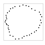
(a) Type A

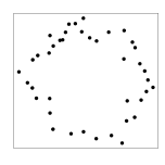
(b) Type B

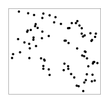
(c) Type C

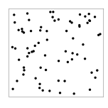
(d) Type D

Figure 6: These glandular structures model typical glands found in prostate biopsy slides, with type A being the least cancerous, and type D being the most cancerous.

To illustrate how functional summaries can be useful in analyzing Gleason data, we conduct a classification analysis with functional summaries. Moreover, we compare the performance in terms of classification based on three functional summaries: the silhouette functions, the landscape functions, and the generalized landscape functions with the triangle kernel. Specifically, we performed $k$-nearest neighbors ($k$NN) classification using the $L_{2}$-metric with $k$ being chosen by the leave-one-out cross-validation (LOOCV). We created a training set consisting of $2000$ simulated glands with $500$ of each type (A–D), and computed persistence diagrams for each observation. Then we generated a test set of 400 simulated glands, $100$ of each type, and computed the corresponding persistence diagrams as well.

Our first analysis was done using the silhouette function. For each persistence diagram, a silhouette function was computed with weights equal to the lifetime of each feature. We apply LOOCV to the training set to choose the number $k$ that minimizes the classification error on the training set. With this choice of $k$, we use the entire training set to construct a $k$NN classifier. To evaluate the performance of this classifier, we use the test set, which leads to an $11.75\%$ overall test classification error, with 47 glands misclassified. Figure 7(b) displays the confusion matrix for the silhouette functions. To demonstrate an approach for visualizing functional summaries, we used multidimensional scaling (MDS; see, .e.g, Friedman et al. 2001) on the silhouette functions to obtain a two-dimensional visualization of the true classes, as seen in Figure 7(a).

This exercise was repeated for landscape functions and generalized landscape functions with the triangle kernel and bandwidths of $h=0.01,0.025,0.05,0.10,$ and $0.25$. Since the landscape approach (generalized landscape) contains several landscape functions, a decision has to be made regarding the number functions to use for each setting. We carried out the simulation study using $1:j$ functions for $j=1,\ldots,6$ (i.e. only using the first function, using only the first and second function, to using the first through sixth functions). For each function type, bandwidth, and number of functions, we apply LOOCV to the training set to choose the tuning parameter $k$, then construct the $k$NN classifier using the training set, and evaluate the accuracy using the test set, as was done for the silhouette functions. Note that in the case of generalized landscape function, we also choose the smoothing bandwidth using LOOCV. The results for the landscape functions are displayed in Table 1, and the results for the best generalized landscape setting (which was the setting with a bandwidth of $h=0.25$) are displayed in Table 2. The best setting for the landscape functions was the case using landscapes $1$ through $6$ with a total number of 57 misclassifications resulting in an overall test classification error rate of 14.25%. The best setting for the generalized landscape functions with $h=0.25$ were the cases using generalized landscapes $1$ through $5$, or $1$ through $6$, with a total number of 39 misclassifications resulting in an overall classification error rate of 9.75%.

Between the silhouette functions, landscape functions, and generalized landscape functions considered in this study, the best generalized landscape functions had the best overall performance in terms of test misclassification error. Most of the errors in classification occurred with gland types B and C where true gland type B was sometimes misclassified as type C, and true gland type C was sometimes misclassified as type B or D. The generalized landscape functions are able to include more details in fewer functions, which may explain why they performed better than the landscapes functions. Silhouette functions contain more layers of information than the landscape functions considered, though the information is averaged based on the lifetime of the features, which may explain their resulting performance between that of the landscape and silhouette functions.

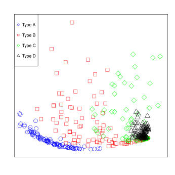
(a) MDS Plot

Type	A	B	C	D
A	99	1	0	0
B	1	86	13	0
C	0	10	76	14
D	0	0	8	92

(b) Confusion Matrix

Figure 7: (left) A two-dimensional MDS plot of the test set using silhouette functions. (right) Silhouette function classification test results. Confusion matrix for the knn classification tests given as percentages using silhouette functions. The rows are the actual type, and the columns are the classified type.

(a) Function orders 1
Type	A	B	C	D
A	98	2	0	0
B	1	82	17	0
C	0	17	69	14
D	0	1	14	85

(b) Function orders 1:2
Type	A	B	C	D
A	98	2	0	0
B	1	86	13	0
C	0	16	71	13
D	0	0	13	87

(c) Function orders 1:3
Type	A	B	C	D
A	98	2	0	0
B	1	84	15	0
C	0	16	70	14
D	0	0	12	88

(d) Function orders 1:4
Type	A	B	C	D
A	98	2	0	0
B	1	82	17	0
C	0	16	70	14
D	0	0	12	88

(e) Function orders 1:5
Type	A	B	C	D
A	99	1	0	0
B	1	83	16	0
C	0	16	70	14
D	0	0	13	87

(f) Function orders 1:6
Type	A	B	C	D
A	99	1	0	0
B	1	85	14	0
C	0	16	70	14
D	0	0	11	89

Table 1: Landscape function gland classification test results. Confusion matrix for the $k$nn classification tests given as percentages using landscape functions. (a)–(f) are the results using function orders 1, 1:2, 1:3, 1:4, 1:5, and 1:6, respectively. The number of nearest neighbors, $k$, was selected using leave-one-out cross-validation for each setting using the training data, and then the test data was used with the optimal $k$ for each setting to obtain the correct classification percentages displayed in these tables. The rows are the actual gland type, and the columns are the classified gland type.

(a) Function orders 1
Type	A	B	C	D
A	100	0	0	0
B	1	89	10	0
C	0	10	77	13
D	0	2	8	90

(b) Function orders 1:2
Type	A	B	C	D
A	100	0	0	0
B	1	89	10	0
C	0	12	71	17
D	0	0	5	95

(c) Function orders 1:3
Type	A	B	C	D
A	100	0	0	0
B	1	89	10	0
C	0	15	72	13
D	0	0	7	93

(d) Function orders 1:4
Type	A	B	C	D
A	100	0	0	0
B	1	91	8	0
C	0	14	76	10
D	0	1	6	93

(e) Function orders 1:5
Type	A	B	C	D
A	100	0	0	0
B	1	91	8	0
C	0	14	78	8
D	0	1	7	92

(f) Function orders 1:6
Type	A	B	C	D
A	100	0	0	0
B	1	91	8	0
C	0	14	78	8
D	0	1	7	92

Table 2: Generalized landscape function gland classification test results. Confusion matrix for the $k$nn classification tests given as percentages using generalized landscape functions with triangle kernels and a bandwidth of 0.25. (a)–(f) are the results using function orders 1, 1:2, 1:3, 1:4, 1:5, and 1:6, respectively. The number or nearest neighbors, $k$, was selected using leave-one-out cross-validation for each setting using the training data, and then the test data was used with the optimal $k$ for each setting to obtain the correct classification percentages displayed in these tables. The rows are the actual gland type, and the columns are the classified gland type.

5.2 Fibrin Data

As noted previously, Pretorius et al. (2009) carried out hypothesis tests between fibrin networks of different species. We use functional summaries of persistence diagrams to carryout two-sample hypothesis tests of a human fibrin network and a monkey fibrin network, both based on images from Pretorius et al. (2009). The modeled human and monkey fibrin images are displayed in Fig. 8, and are produced by removing the white scale bar from the original images of Pretorius et al. (2009) (see Fig. 2 for the original human fibrin network). The modeling carried out is a minimal amount of smoothing to reduce the high contrasts of the image. Namely, local quadratic regression is used with an adaptive bandwidth that includes the 0.1% of the nearest neighbors of the point of interest. The corresponding persistence diagrams use upper-level set filtrations on the modeled images, and are displayed in Fig. 9. Both diagrams have similar features with $H_{0}$ features appearing early in the filtration, which die off and produce $H_{1}$ features.

Before jumping into the fibrin dataset, we carryout a simulation study using, what we refer to as, the Pickup Sticks Simulator (STIX), in order to check the performance of the proposed two-sample tests using different types of functional summaries when the ground truth is known. The goal of STIX is to mimic some of the spatially complex features apparent in the fibrin data.

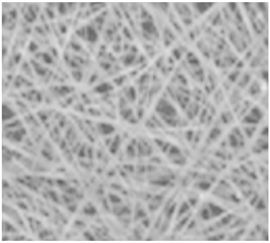
(a) Modeled human fibrin

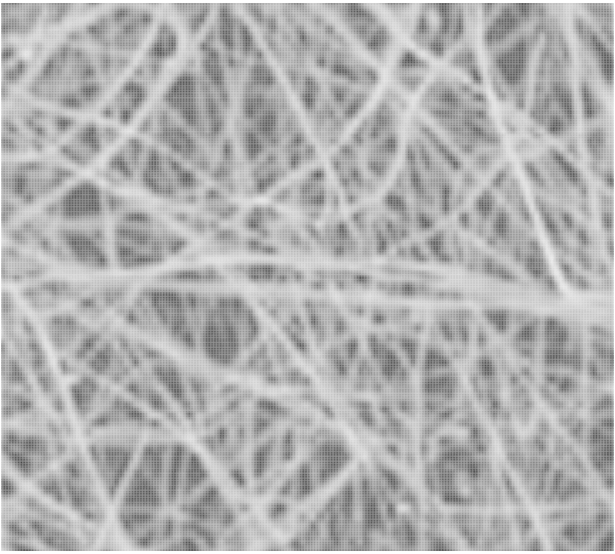
(b) Modeled monkey fibrin

Figure 8: Modeled human fibrin network (left) and monkey fibrin network (right); original images are from Pretorius et al. (2009). The modeling step uses local quadratic regression with an adaptive bandwidth that includes the 0.1% of the nearest neighbors of the point of interest.

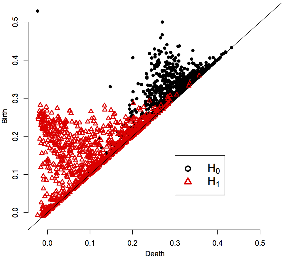
(a) Human fibrin persistence diagram

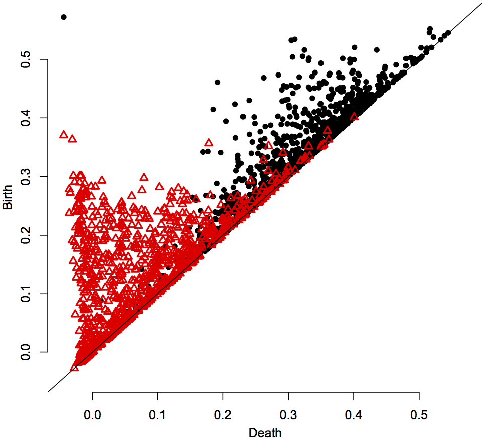
(b) Monkey fibrin persistence diagram

Figure 9: Persistence diagrams for the modeled human (left) and monkey (right) fibrin networks displayed in Fig. 8 computed using an upper-level set filtration on the modeled images.

5.2.1 Pick-up Sticks Simulation Data

Motivated by fibrin networks, we developed data simulator that attempts to mimic some of the complicated spatial structure of fibrin. The STIX generates data that resembles the web-like features of the fibrin networks. The following is the STIX recipe supposing $n$ segments, or sticks, are desired in the image. Two sets of $n$ points are randomly sampled from a Uniform distribution with segments drawn between points in the same position of the two lists of random numbers. The thickness of each segment is randomly drawn from a $\chi^{2}$ distribution with thickness = $t$ degrees of freedom. Fig. 10 displays realizations of STIX with two different average thicknesses, 5 and 6.

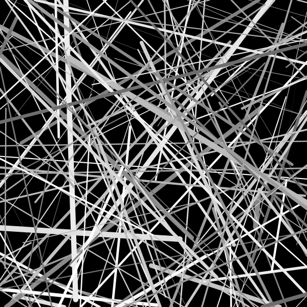
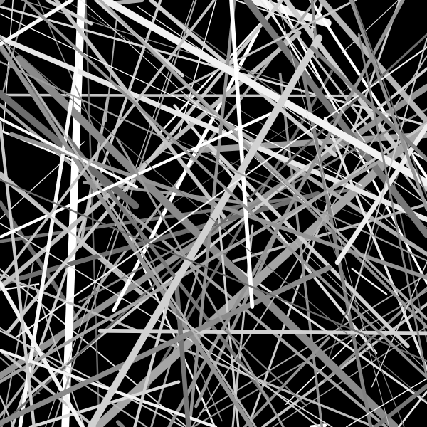
Figure 10: Realizations of the Pick-up Sticks Simulation Data (STIX) with average thicknesses of (left) 5 and (right) 6.

We carryout a simulation study using STIX to check the performance of the two-sample hypothesis tests using landscape and generalized landscape functions. Using the two-sample test framework from Section 4.4, and Equation (13) in particular, we generate images from two populations with the difference in the two populations being the average thickness of the segments via the degrees of freedom of the $\chi^{2}$ distribution.

For the simulation study, $\mathcal{P}_{F,1}$ is the null population, and a thickness of $t_{1}=5$ is used. The alternative populations consider a range of thicknesses, $t_{2}=5,5.25,5.5,5.75,6,7,8$, where $t_{2}=5$ is used to check the power of the test. For null thickness, $t_{1}$ and alternative thickness $t_{2}$, 100 repetitions of the following are carried out. First, 12 STIX images are produced using both $t_{1}$ and $t_{2}$ (24 images total). Then each image is smoothed using local quadratic regression with an adaptive bandwidth that includes the 0.1% of the nearest neighbors, and a persistence diagram is computed using upper-level sets on the modeled images. Then landscape functions and generalized landscapes with the triangle kernel and varying bandwidths (0.01, 0.025, 0.05, 0.10) were computed. Permutation p-values were computed using the permutation test framework introduced in Section 4.4 using 10,000 random permutations.

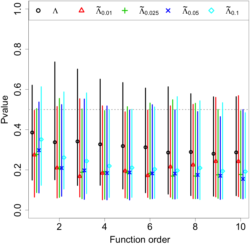
(b) Hom. dim=1, 5 vs. 5.25

(c) Hom. dim=1, 5 vs. 5.5

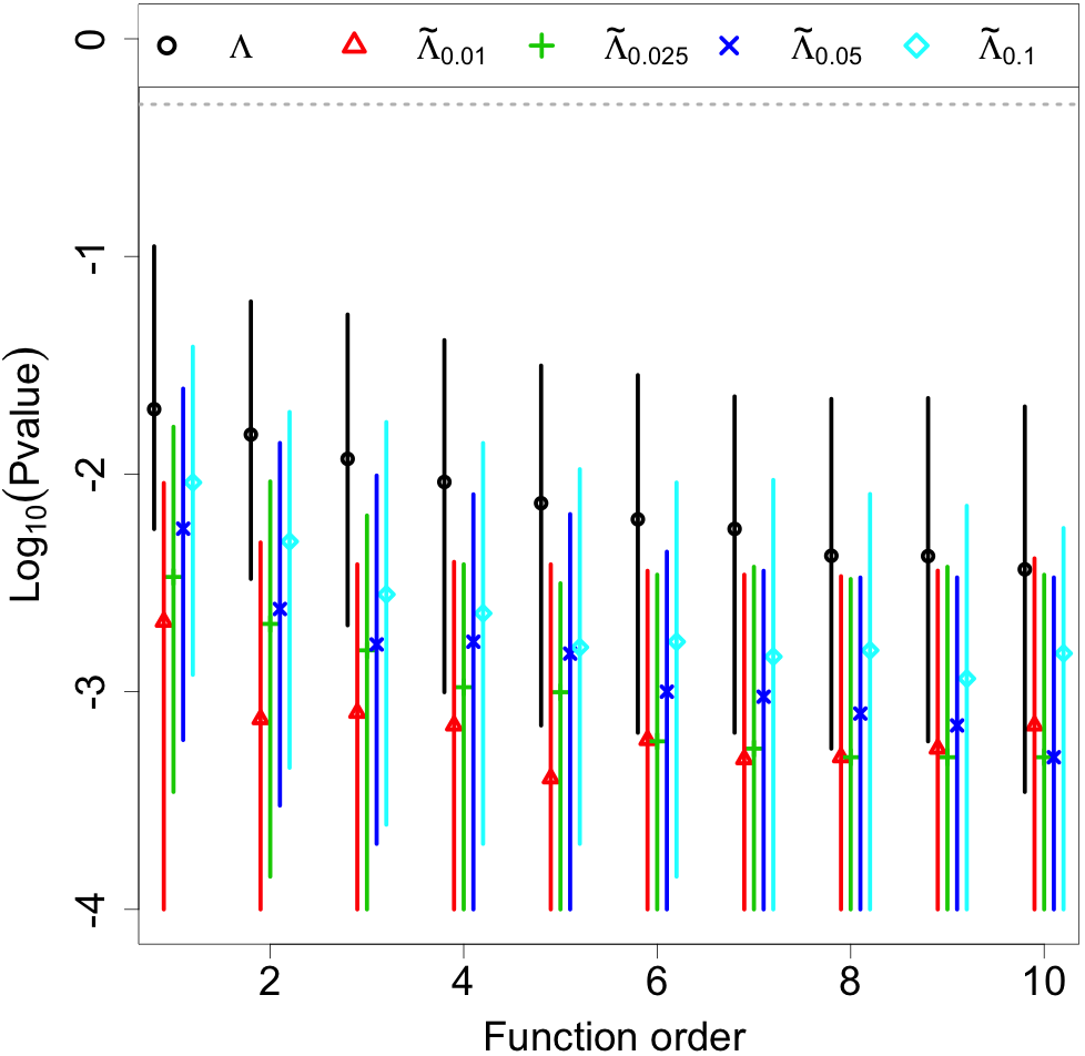
(d) Hom. dim=1, 5 vs. 5.75

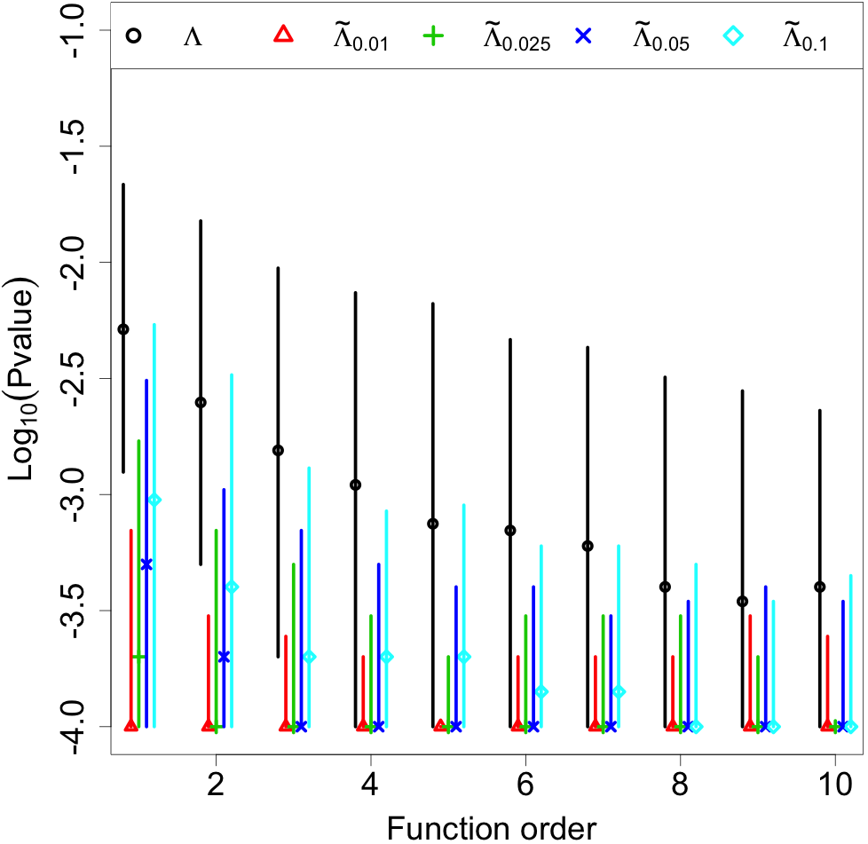
(e) Hom. dim=1, 5 vs. 6

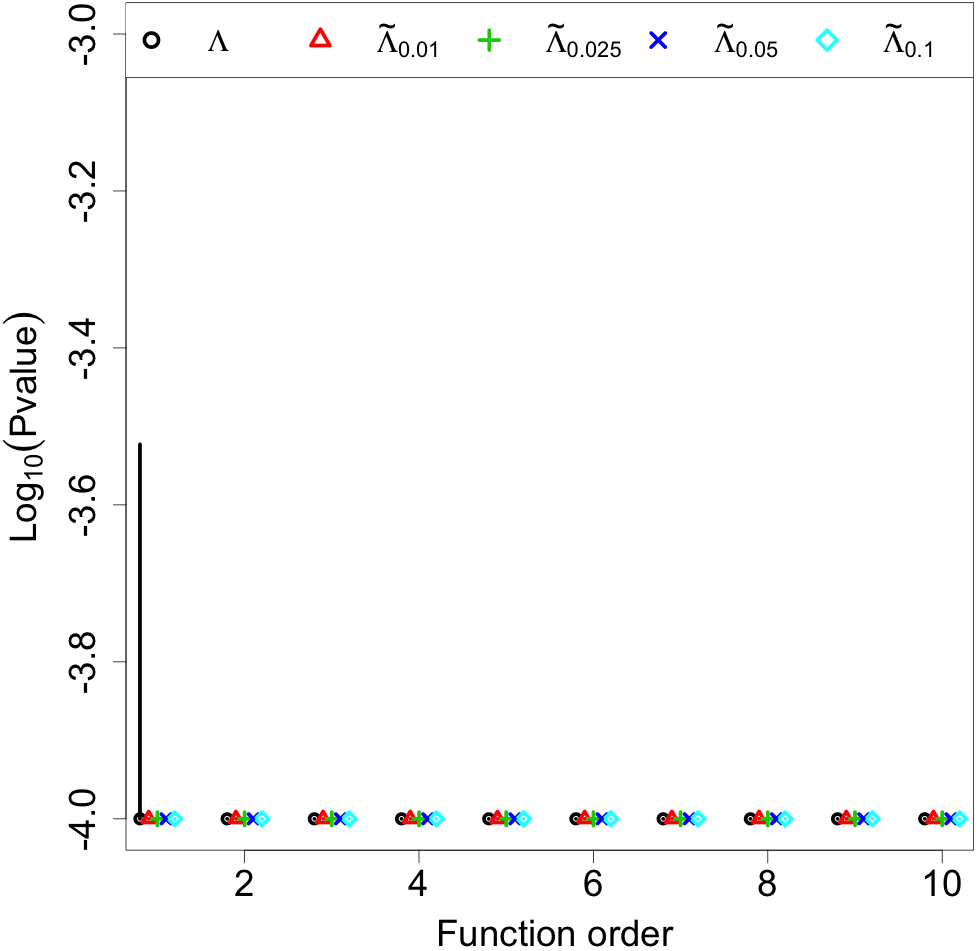
(f) Hom. dim=1, 5 vs. 7

Figure 14: STIX simulation results for Homology dimension 1. The median permutation p-values (a) - (c) and $\log_{10}$(pvalues) (d) - (f) are plotted along with their interquartile range (the vertical lines) for two-sample hypothesis tests comparing samples drawn from the null population, $\mathcal{P}_{F,1}$, with an average thickness of $t_{1}=5$. The alternative hypotheses include average thicknesses of $t_{2}=5,5.25,5.5,5.75,6,7,8$, corresponding to images (a) - (f), respectively (except average thickness of 8 is not displayed). The permutation p-values are based on 100 repetitions of 12 STIX images drawn from the null and alternative hypothesis, with 10,000 random permutations. The different plot colors and symbols represent the different functions and bandwidths considered; the function order is the ordering of the landscape and generalized landscape functions (see the discussion around Equation (2)).

The results of this simulation study for $t_{2}=5$ and $5.5$ using the 1st homology dimension are displayed in Fig. 11 with the remaining results displayed in Appendix A. The median p-values or $\log_{10}$(p-values) are displayed along with their interquartile range for 10 function orders of the landscapes and generalized landscapes considered. Fig. 11(a) displays the results for the case where the null and alternative populations are the same (with an average thickness of 5), all methods perform well with p-values distributed around 0.5. As the alternative population’s thickness increases, all methods have p-values that get smaller. The landscape function orders tend to have larger p-values than the generalized landscape function orders, with the generalized landscapes with the smallest bandwidth considered, 0.01 (red triangles), tending to have the lowest p-values among the generalized landscapes. The results for the case with the alternative hypothesis average thickness of 8 are not displayed since all tests resulted in the minimum p-value. In Appendix A, the simulation results for the 0th homology dimension are displayed in Fig. 13 and rest of the results for the 1st homology dimension are displayed in Fig. 14.

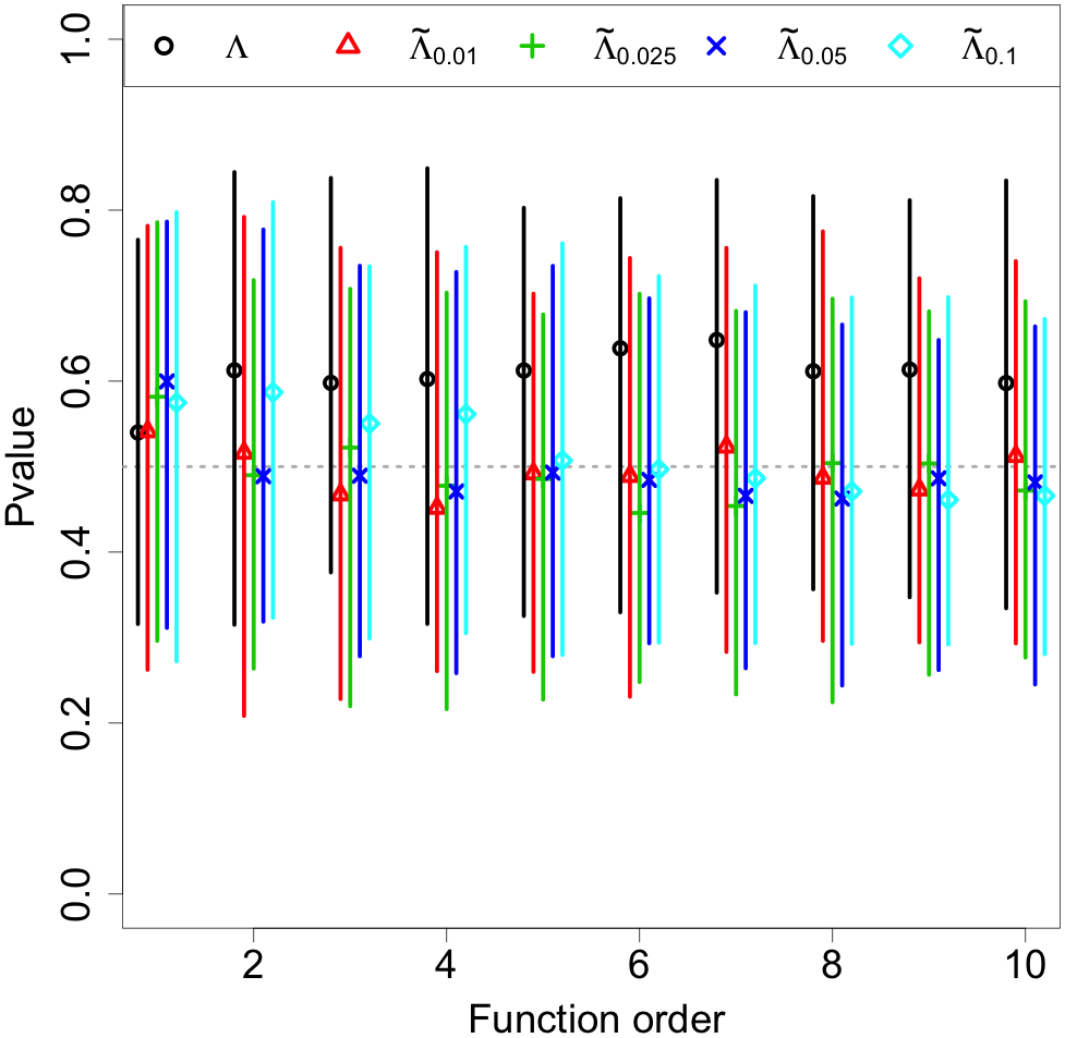
(a) Homology dim=1, Thickness 5 vs. 5

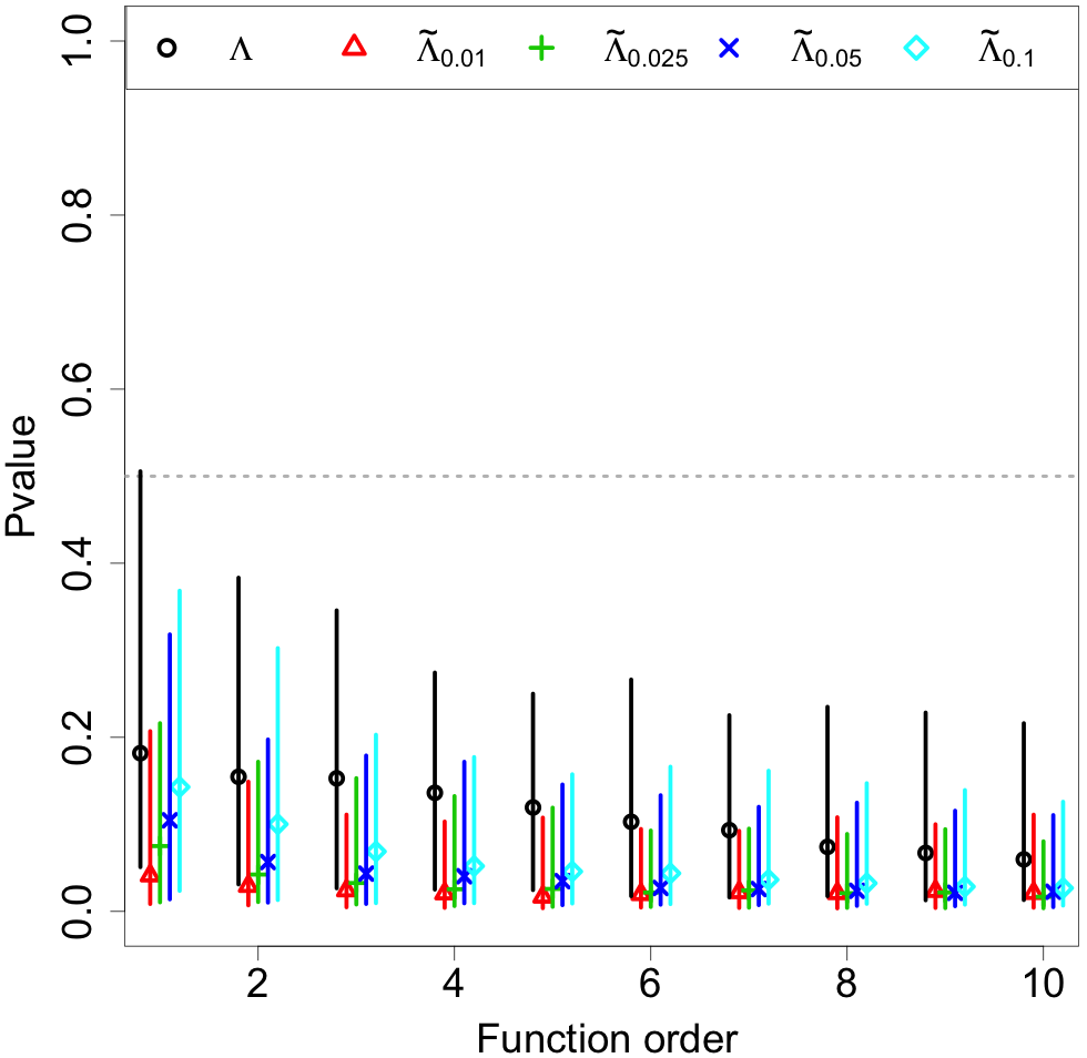
(b) Homology dim=1, Thickness 5 vs. 5.5

Figure 11: STIX simulation results for Homology dimension 1. The median permutation p-values are plotted along with their interquartile range (the vertical lines) for two-sample hypothesis tests comparing samples drawn from the null population, $\mathcal{P}_{F,1}$, with an average thickness of $t_{1}=5$. The alternative hypotheses include average thicknesses of $t_{2}=5$ and $5.5$, corresponding to plots A and B, respectively. The permutation p-values are based on 100 repetitions of 12 STIX images drawn from the null and alternative hypothesis, with 10,000 random permutations. The different plot colors and symbols represent the different functions and bandwidths considered; the function order is the ordering of the landscape and generalized landscape functions (see the discussion around Equation (2)). The results for $t_{2}=5,5.25,5.5,5.75,6,7$ are displayed in Fig. 14.

5.2.2 Fibrin Data Results

In order to carryout a two-sample test of the human and monkey fibrin images from Pretorius et al. (2009), the images are first divided into 12 sub-images (3 by 4) because only a single image of each group was available. The sub-images are then smoothed using local quadratic regression with an adaptive bandwidth that includes the 0.1% of the nearest neighbors, and a persistence diagram is computed using upper-level sets on the modeled sub-images. Then landscape functions and generalized landscapes with the triangle kernel and varying bandwidths (0.01, 0.025, 0.05, 0.10) were computed for each sub-image, and permutation tests were carried out. The results are displayed in Fig. 12. For homology dimension 0, the generalized landscapes tended to have lower p-values than the landscapes for all function orders except all methods had the minimum p-value for the first function order. For function orders 2 - 10, the generalized landscape with the smallest bandwidth considered (0.01) tended to have the next highest p-values, and the generalized landscape with the largest bandwidth considered tended to have the lowest p-values. For homology dimension 1, all of the generalized landscapes achieved the minimum p-value, and the landscape p-values tended to be slightly higher.

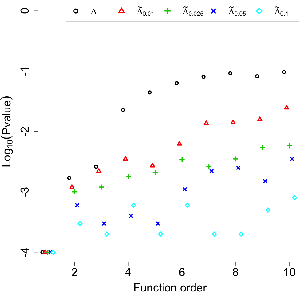
(a) Homology dim=$0$

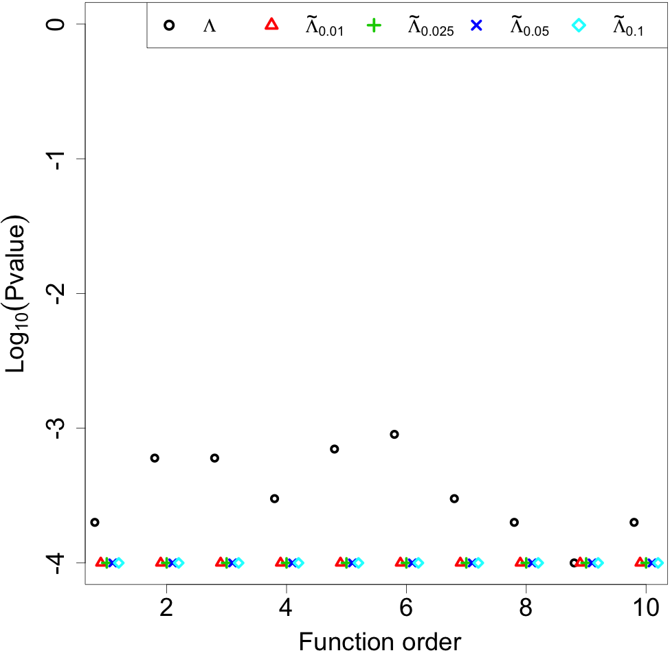
(b) Homology dim=$1$

Figure 12: Human vs. monkey fibrin results. Log₁₀ p-values from the two-sample permutation hypothesis tests using the images of monkey and human fibrin from Pretorius et al. (2009) (a modeled version of these images are displayed in Fig. 8). The human and monkey dataset were composed of $12$ images each (the original image divided). The tests were carried out using 10,000 random permutations. The different plot colors and symbols represent the different functions and bandwidths considered; the function order is the ordering of the landscape and generalized landscape functions (see the discussion around Equation (2)).

6 Discussion

Statistical analysis of persistence diagrams is challenging, which has led to the development of a variety of functional transformations of the persistence diagrams. We reviewed the popular functional summaries proposed in the literature. For the landscape function, we generalize the formulation in order to allow more flexibility in the shape and width of the kernel, rather than requiring isosceles right triangles.

By putting analysis of persistence diagrams into a functional framework, we explained how the many tools of functional data analysis can be employed for their analysis. We find that the average of functional summaries is a consistent estimator of the population mean function, which allows us to view the sample mean functional summary as an estimator for this population characteristic. We analyze some basic functional convergence theorems for the persistence functional summaries, including a pointwise convergence and a uniform convergence theorem. Moreover, we propose a bootstrap procedure for assessing the uncertainty of the the sample mean functional summary and show that one can construct an asymptotically valid confidence band of the underlying population mean functional summary. Using the proposed framework and the convergence theorems, we show that one can conduct various statistical analyses of the data such as constructing a prediction region for future functional summaries, performing a two-sample test to determine if two sets of persistence diagrams are from the same population, classifying persistence diagrams into multiple classes, partitioning persistence diagrams into clusters, and visualizing the relationship between several persistence diagrams.

In the simulation studies of Section 5, the proposed generalized landscapes performed better than the traditional landscapes and the silhouettes in terms of test classification error for the Gleason data, and generally had lower p-values than the traditional landscapes in the two-sample hypothesis tests for the STIX simulation study (when the alternative hypothesis was true). However, the generalized landscapes come with the cost of needing to select a kernel and, more importantly, the bandwidth. One benefit of the generalized landscape formulation is that more information of the persistence diagram can be packed in fewer function orders, which can aid in dimension reduction. Before carrying out the two-sample hypothesis tests on the fibrin network images from Pretorius et al. (2009), we developed a new data simulator, STIX, which has a similar complicated spatial structure to the fibrin network and provided an interesting testing ground for the proposed methods. Without needing to measure the widths of any of the sticks, the proposed tests based on the persistence functional summaries were able to detect small differences in the sampled populations when the two populations actually differed, and detected no difference in the case where the two samples came from the same population.

Acknowledgments:

On behalf of all authors, the corresponding author states that there is no conflict of interest. Berry and Fasy acknowledges supported by NIH and NSF under Grant Numbers NSF DMS 1664858 and NSF DMS 1557716. Chen is supported by NIH grant number U01 AG016976. Cisewski-Kehe thanks the great staff and available resources at the Yale Center for Research Computing. Fasy is additionally supported by NSF CCF 1618605.

Appendix A STIX simulation results

For completeness, the full results for the STIX simulation study from §5.2.1 are displayed in Fig. 13 and 14. These are the full results corresponding to the 0th and 1st homology dimension, respectively, while a subset of the results for the 1st homology dimension are displayed in Fig. 11 and discussed in the main text.

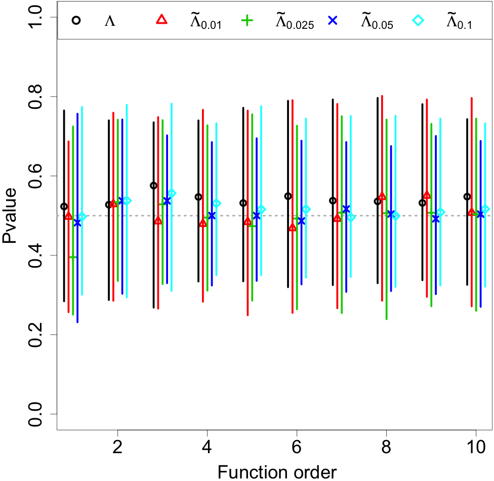
(a) Hom. dim=0, 5 vs. 5

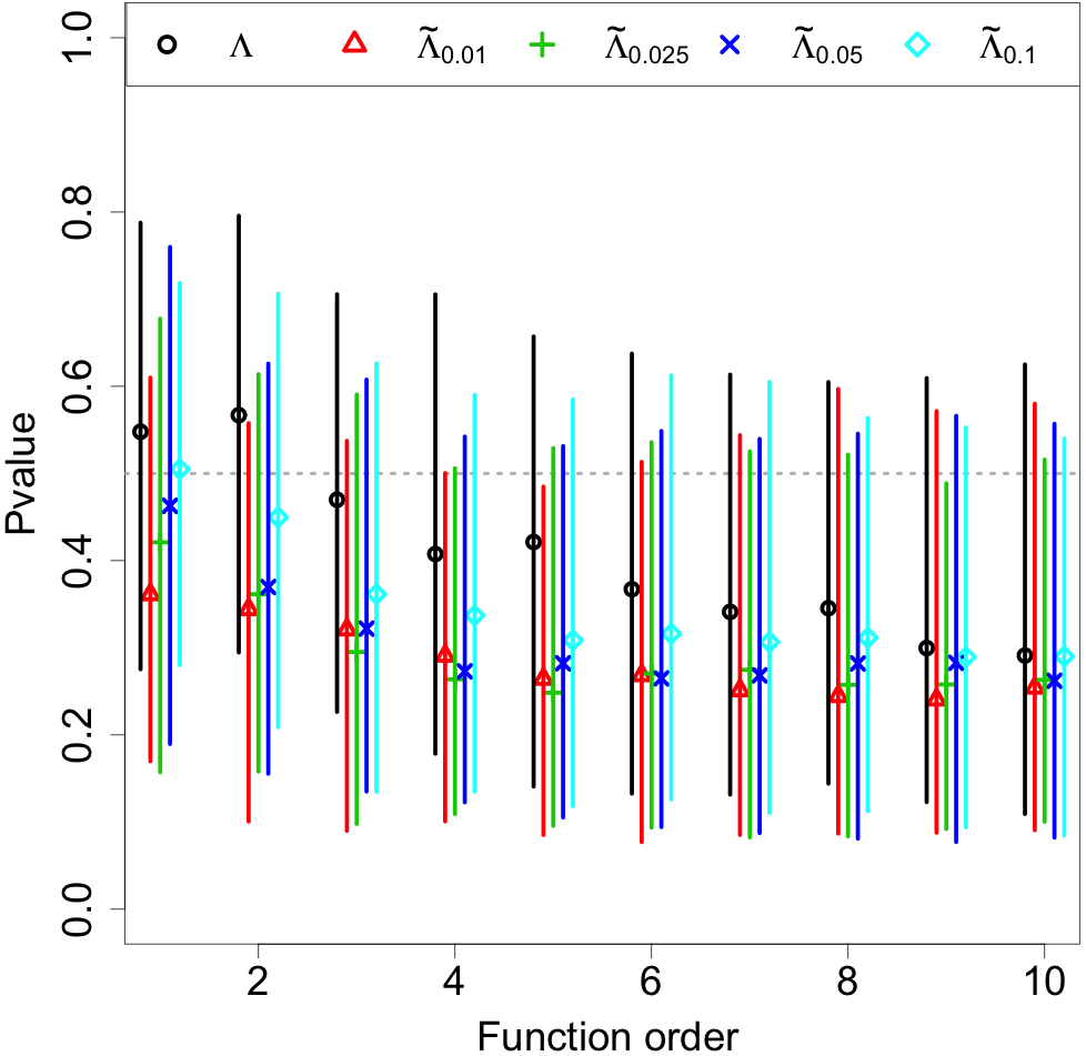
(b) Hom. dim=0, 5 vs. 5.25

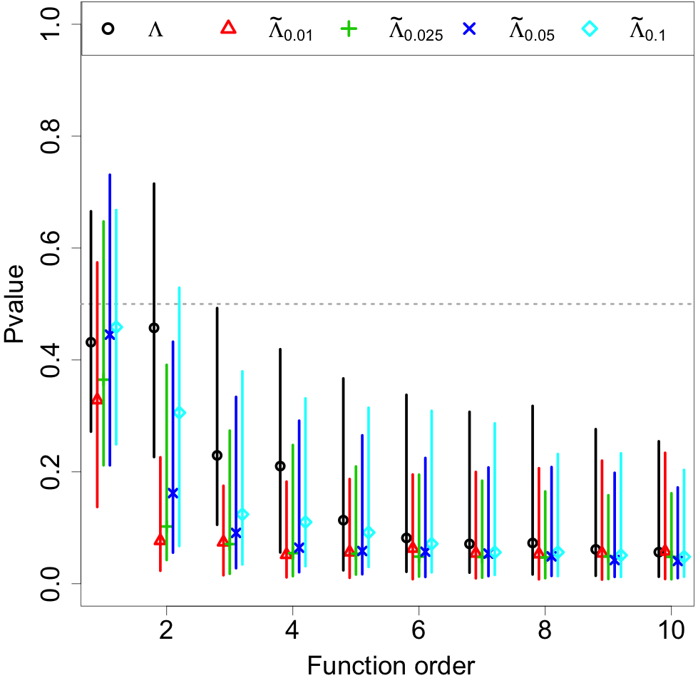
(c) Hom. dim=0, 5 vs. 5.5

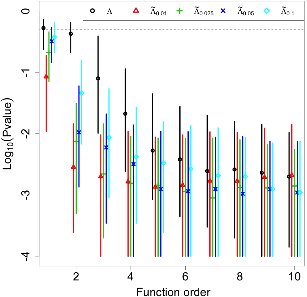
(d) Hom. dim=0, 5 vs. 5.75

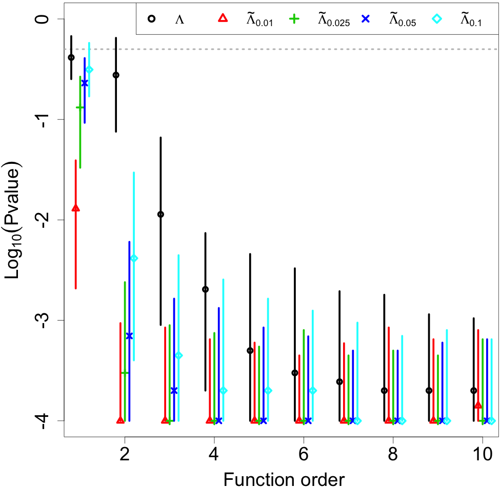
(e) Hom. dim=0, 5 vs. 6

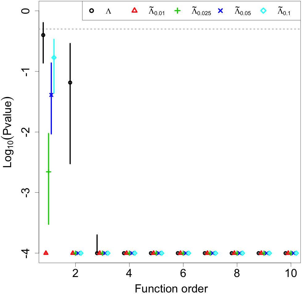
(f) Hom. dim=0, 5 vs. 7

Figure 13: STIX simulation results for Homology dimension 0. The median permutation p-values (a) - (c) and $\log_{10}$(pvalues) (d) - (f) are plotted along with their interquartile range (the vertical lines) for two-sample hypothesis tests comparing samples drawn from the null population, $\mathcal{P}_{F,1}$, with an average thickness of $t_{1}=5$. The alternative hypotheses include average thicknesses of $t_{2}=5,5.25,5.5,5.75,6,7,8$, corresponding to images (a) - (f), respectively (except average thickness of 8 is not displayed). The permutation p-values are based on 100 repetitions of 12 STIX images drawn from the null and alternative hypothesis, with 10,000 random permutations. The different plot colors and symbols represent the different functions and bandwidths considered; the function order is the ordering of the landscape and generalized landscape functions (see the discussion around Equation (2)).

(a) Hom. dim=1, 5 vs. 5

Appendix B Proofs

The proofs from the propositions of Section 4 are presented below.

Proof

of Proposition 1. This proof uses ideas from Rubin (1956) and Yuan (1997).

Let $\epsilon>0$ be given. Because $\mathcal{B}_{F}$ is equicontinuous, the collection of differences

$$\mathcal{B}_{\Delta}=\{\widehat{F}-\bar{F}:n=1,2,\cdots\}$$

is also equicontinuous. Since $\mathbb{T}$ is compact, there exists a number $M>0$ and points $t_{1},\cdots,t_{M}\in\mathbb{T}$ such that

$$\sup_{\Delta\in\mathcal{B}_{\Delta}}\min_{j=1,\cdots,M}|\Delta(t)-\Delta(t_{j})|<\epsilon/2.$$

Namely, $t_{1},\cdots,t_{M}$ forms a $\epsilon/2$-covering of $\mathcal{B}_{\Delta}$.

Let $\Delta_{n}(t)=\widehat{F}(t)-\bar{F}(t)$, and note that $\Delta_{n}\in\mathcal{B}_{\Delta}$. Then

$$\sup_{t\in\mathbb{T}}|\widehat{F}(t)-\bar{F}(t)| =\sup_{t\in\mathbb{T}}|\Delta_{n}(t)|$$

$$\leq\sup_{t\in\mathbb{T}}\min_{j\in 1,\cdots,M}|\Delta_{n}(t)-\Delta_{n}(t_{j})|+\sup_{j\in 1,\cdots,M}|\Delta_{n}(t_{j})|$$

$$\leq\epsilon/2+\sup_{j\in 1,\cdots,M}|\Delta_{n}(t_{j})|.$$

By Equation (5), every $t\in\mathbb{T}$ satisfies $\mbox{$\mathbb{E}$}|F_{i}(t)|<\infty$ so by the strong law of large number,

$$|\Delta_{n}(t_{j})|\overset{a.s.}{\rightarrow}0$$

for every $j=1,\cdots,M$ and this implies that for any $\delta>0$, there exists $N>0$ such that

$$P\left(\sup_{n\geq N}|\Delta_{n}(t_{j})|>\frac{\epsilon}{2M}\right)<\frac{\delta}{M}$$

for every $j=1,\cdots,M$.

As a result,

$$P\left(\sup_{t\in\mathbb{T}}|\widehat{F}(t)-\bar{F}(t)|>\epsilon\right) \leq P\left(\epsilon/2+\sup_{j\in 1,\cdots,M}|\Delta_{n}(t_{j})|>\epsilon\right)$$

$$\leq P\left(\sup_{n\geq N}\sup_{j\in 1,\cdots,M}|\Delta_{n}(t_{j})|>\frac{\epsilon}{2}\right)$$

$$\leq\sum_{j=1}^{M}P\left(\sup_{n\geq N}|\Delta_{n}(t_{j})|>\frac{\epsilon}{2M}\right)$$

$$\leq\delta$$

and the result follows.

Proof

of Proposition 2.

Note that by Equation (5), the functional summary satisfies

$$\sup_{t\in\mathbb{T}}{\sf Var}(F_{i}(t))\leq\sup_{t\in\mathbb{T}}\mbox{$\mathbb{E}$}(F^{2}_{i}(t))\leq\bar{U}^{2}<\infty.$$

Pointwise normality. The first assertion $\sqrt{n}(\widehat{F}(t)-\bar{F}(t))\rightarrow N(0,\sigma^{2}(t))$ follows from the usual central limit theorem.

Normality of integrated difference. To show the normality for the integrated difference, note that

$$\sqrt{n}\int(\widehat{F}(t)-\bar{F}(t))dt =\sqrt{n}\int\left(\frac{1}{n}\sum_{i=1}^{n}F_{i}(t)-\bar{F}(t)\right)dt$$

$$=\sqrt{n}\frac{1}{n}\sum_{i=1}^{n}\underbrace{\int\left(F_{i}(t)-\bar{F}(t)\right)dt}_{=Y_{i}}$$

$$=\sqrt{n}\bar{Y}_{n},$$

where $\bar{Y}_{n}=\frac{1}{n}\sum_{i=1}^{n}Y_{i}$ and $Y_{1},\cdots,Y_{n}$ are IID with mean $\mbox{$\mathbb{E}$}(Y_{i})=0$ and variance

$${\sf Var}(Y_{i})=\int{\sf Var}(F_{i}(t))dt=\int\sigma^{2}(t)dt<\infty.$$

Thus, by the usual central limit theorem again, we obtain the normality.

Convergence to a Gaussian process. The assumption in Equation (6) along with Theorem 2.5 in Kosorok (2007) implies that the class $\mathcal{W}$ is Donsker, which implies that the empirical process converges to a Gaussian process.

Proof

of Proposition 3. Because Equation (6) implies that the class $\mathcal{W}$ is Donsker, this proposition is a well-known result in the empirical process theory. For instance, see the discussion on page 21 of Kosorok (2007). Here we briefly highlight the basic idea.

By Proposition 3 and the continuous mapping theorem (see, e.g., page 16 of Kosorok (2007)),

$$\sqrt{n}\sup_{t\in\mathbb{T}}|\widehat{F}(t)-\bar{F}(t)|\overset{D}{\rightarrow}\sup_{t\in\mathbb{T}}|\mathbb{B}(t)|.$$

In the case of the bootstrap, using the same proposition but now apply it to the bootstrap version, we obtain

$$\sqrt{n}\sup_{t\in\mathbb{T}}|\widehat{F}^{*}(t)-\widehat{F}(t)|\overset{D|F^{\otimes n}}{\rightarrow}\sup_{t\in\mathbb{T}}|\mathbb{B}(t)|,$$

where $\overset{D|F^{\otimes n}}{\rightarrow}$ denotes convergences in distribution given $F_{1},\cdots,F_{n}$.

Therefore, the bootstrap quantile converges to the corresponding quantile of the original difference.

Proof

of Proposition 4. This proof consists of two parts. In the first part, we prove that $\widehat{q}_{\gamma}\overset{P}{\rightarrow}q_{\gamma}$. In the second part, we prove the desired result.

Part 1. Given $F_{1},\cdots,F_{n}$, we define

$$\widehat{Q}(t)=\frac{1}{n}\sum_{i=1}^{n}I(d(F_{i},\bar{F})\leq t)$$

to be the empirical version of $Q(t)$ and define

$$\widetilde{q}_{\gamma}:\widehat{Q}(\widetilde{q}_{\gamma})=\gamma,$$

to be the corresponding $\gamma$ quantile.

Because $\widehat{Q}$ is just the empirical distribution function (EDF) of $Y_{1},\cdots,Y_{n}$ where $Y_{i}=d(F_{i},\bar{F})$ and $Q(t)$ is the cumulative distribution function (CDF) of $Y_{i}$,

$$\sup_{t}|\widehat{Q}(t)-Q(t)|=O_{P}\left(\frac{1}{\sqrt{n}}\right).$$

By the mean value theorem and the fact that $\widehat{Q}(\widetilde{q}_{\gamma})-Q(\widetilde{q}_{\gamma})=o_{P}(1)$,

$$\widehat{Q}(\widetilde{q}_{\gamma})-Q(\widetilde{q}_{\gamma}) =Q(q_{\gamma})-Q(\widetilde{q}_{\gamma})$$

$$=Q^{\prime}(q_{\gamma}^{*})(q_{\gamma}-\widetilde{q}_{\gamma})$$

for some $q_{\gamma}^{*}\in[q_{\gamma},\widetilde{q}_{\gamma}]$. By assumption, $Q^{\prime}(q_{\gamma}^{*})\geq q_{0}>0$ so

$$|q_{\gamma}-\widetilde{q}_{\gamma}|\leq\frac{1}{q_{0}}\left|\widehat{Q}(\widetilde{q}_{\gamma})-Q(\widetilde{q}_{\gamma})\right|=O_{P}\left(\frac{1}{\sqrt{n}}\right).$$

Now, because $\max{i=1,\cdots,n}|d(F_{i},\bar{F})-d(F_{i},\widehat{F})|\leq d(\bar{F},\widehat{F})$, $\widetilde{q}_{\gamma}$, the quantile of $d(F_{1},\bar{F}),\cdots,d(F_{n},\bar{F})$, and $\widehat{q}_{\gamma}$, the quantile of $d(F_{1},\widehat{F}),\cdots,d(F_{n},\widehat{F})$, are bounded by

$$|\widetilde{q}_{\gamma}-\widehat{q}_{\gamma}|\leq d(\bar{F},\widehat{F}).$$

which implies

$$|\widehat{q}_{\gamma}-q_{\gamma}|=O_{P}\left(\frac{1}{\sqrt{n}}\right)+d(\bar{F},\widehat{F}).$$

Part 2. Let

$$\widehat{A}_{\gamma}=P(F_{\sf new}\subset\widehat{\mathcal{F}}_{\gamma}|F_{1},\cdots,F_{n})=P(d(F_{\sf new},\widehat{F})\leq\widehat{q}_{\gamma}|F_{1},\cdots,F_{n}).$$

be the probability of interest. By the triangular inequality,

$$|d(F_{\sf new},\bar{F})-d(F_{\sf new},\widehat{F})|\leq d(\bar{F},\widehat{F}).$$

Thus,

$$A_{\gamma} =P(d(F_{\sf new},\widehat{F})\leq\widehat{q}_{\gamma}|F_{1},\cdots,F_{n})$$

$$\geq P(d(F_{\sf new},\bar{F})\leq\widehat{q}_{\gamma}-d(\widehat{F},\bar{F})|F_{1},\cdots,F_{n})$$

$$=Q(\widehat{q}_{\gamma}-d(\widehat{F},\bar{F}))$$

$$\geq Q\left(q_{\gamma}-2d(\widehat{F},\bar{F})+O_{P}\left(\frac{1}{\sqrt{n}}\right)\right)$$

$$=Q(q_{\gamma})+O_{P}\left(\left(\frac{1}{\sqrt{n}}\right)+d(\widehat{F},\bar{F})\right).$$

$$A_{\gamma} =P(d(F_{\sf new},\widehat{F})\leq\widehat{q}_{\gamma}|F_{1},\cdots,F_{n})$$

$$\leq P(d(F_{\sf new},\bar{F})\leq\widehat{q}_{\gamma}+d(\widehat{F},\bar{F})|F_{1},\cdots,F_{n})$$

$$=Q(\widehat{q}_{\gamma}+d(\widehat{F},\bar{F}))$$

$$\leq Q\left(q_{\gamma}+2d(\widehat{F},\bar{F})+O_{P}\left(\frac{1}{\sqrt{n}}\right)\right)$$

$$=Q(q_{\gamma})+O_{P}\left(\left(\frac{1}{\sqrt{n}}\right)+d(\widehat{F},\bar{F})\right).$$

Thus,

$$A_{\gamma}=P(F_{\sf new}\subset\widehat{\mathcal{F}}_{\gamma}|F_{1},\cdots,F_{n})=\underbrace{Q(q_{\gamma})}_{=\gamma}+O_{P}\left(\left(\frac{1}{\sqrt{n}}\right)+d(\widehat{F},\bar{F})\right),$$

which completes the proof.

References

- (1)
- Abdollahi et al. (2012) Abdollahi, A., Meysamie, A., Sheikhbahaei, S., Ahmadi, A., Tabriz, H. M., Bakhshandeh, M. & Hosseinzadeh, H. (2012), ‘Inter/intra-observer reproducibility of Gleason scoring in prostate adenocarcinoma in Iranian pathologists’, Urology J. 9(2), 486–490.
- Adams et al. (2017) Adams, H., Emerson, T., Kirby, M., Neville, R., Peterson, C., Shipman, P., Chepushtanova, S., Hanson, E., Motta, F. & Ziegelmeier, L. (2017), ‘Persistence images: A stable vector representation of persistent homology’, The J. of Machine Learning Research 18(1), 218–252.
- Adcock et al. (2016) Adcock, A., Carlsson, E. & Carlsson, G. (2016), ‘The ring of algebraic functions on persistence bar codes’, Homology, Homotopy and Applications 18(1).
- Adler et al. (2010) Adler, R. J., Bobrowski, O., Borman, M. S., Subag, E. & Weinberger, S. (2010), Persistent homology for random fields and complexes, in ‘Borrowing Strength: Theory Powering Applications – A Festschrift for Lawrence D. Brown’, Vol. 6, Institute of Mathematical Statistics, pp. 124–143.
- Bendich et al. (2016) Bendich, P., Marron, J. S., Miller, E., Pieloch, A. & Skwerer, S. (2016), ‘Persistent homology analysis of brain artery trees’, The Annals of Applied Statistics 10(1), 198.
- Biscio & Møller (2016) Biscio, C. & Møller, J. (2016), ‘The accumulated persistence function, a new useful functional summary statistic for topological data analysis, with a view to brain artery trees and spatial point process applications’, arXiv preprint arXiv:1611.00630 .
- Bubenik (2015) Bubenik, P. (2015), ‘Statistical topological data analysis using persistence landscapes’, J. of Machine Learning Research 16(1), 77–102.
- Campbell et al. (2009) Campbell, R. A., Overmyer, K. A., Selzman, C. H., Sheridan, B. C. & Wolberg, A. S. (2009), ‘Contributions of extravascular and intravascular cells to fibrin network formation, structure, and stability’, Blood 114(23), 4886–4896.
- Carlsson (2009) Carlsson, G. (2009), ‘Topology and data’, Bulletin of the American Mathematical Society 46(2), 255 – 308.
- Center et al. (2012) Center, M. M., Jemal, A., Lortet-Tieulent, J., Ward, E., Ferlay, J., Brawley, O. & Bray, F. (2012), ‘International variation in prostate cancer incidence and mortality rates’, European Urology 61(6), 1079–1092.
- Chazal et al. (2014) Chazal, F., Fasy, B. T., Lecci, F., Rinaldo, A. & Wasserman, L. (2014), Stochastic convergence of persistence landscapes and silhouettes, in ‘Proceedings of the Thirtieth Annual Symposium on Computational Geometry’, ACM, p. 474.
- Chen et al. (2015) Chen, Y.-C., Wang, D., Rinaldo, A. & Wasserman, L. (2015), ‘Statistical analysis of persistence intensity functions’, arXiv preprint arXiv:1510.02502 .
- Ciollaro et al. (2014) Ciollaro, M., Genovese, C., Lei, J. & Wasserman, L. (2014), ‘The functional mean-shift algorithm for mode hunting and clustering in infinite dimensions’, arXiv preprint arXiv:1408.1187 .
- Cisewski et al. (2014) Cisewski, J., Croft, R. A., Freeman, P. E., Genovese, C. R., Khandai, N., Ozbek, M. & Wasserman, L. (2014), ‘Non-parametric 3d map of the intergalactic medium using the lyman-alpha forest’, Monthly Notices of the Royal Astronomical Society 440(3), 2599–2609.
- Cohen-Steiner et al. (2007) Cohen-Steiner, D., Edelsbrunner, H. & Harer, J. (2007), ‘Stability of persistence diagrams’, Discrete & Computational Geometry 37(1), 103–120.
- Crawford et al. (2016) Crawford, L., Monod, A., Chen, A. X., Mukherjee, S. & Rabadán, R. (2016), ‘Topological summaries of tumor images improve prediction of disease free survival in glioblastoma multiforme’, arXiv preprint arXiv:1611.06818 .
- Edelsbrunner & Harer (2008) Edelsbrunner, H. & Harer, J. (2008), ‘Persistent homology - a survey’, Contemporary Mathematics 453, 257 – 282.
- Edelsbrunner et al. (2002) Edelsbrunner, H., Letscher, D. & Zomorodian, A. (2002), ‘Topological persistence and simplification’, Discrete and Computational Geometry 28(4), 511–533.
- Edelsbrunner & Morozov (2012) Edelsbrunner, H. & Morozov, D. (2012), Persistent homology: Theory and practice, in ‘Proceedings of the European Congress of Mathematics’, pp. 31–50.
- Engers (2007) Engers, R. (2007), ‘Reproducibility and reliability of tumor grading in urological neoplasms’, World J. of Urology 25(6), 595–605.
- Epstein et al. (2016) Epstein, J. I., Egevad, L., Amin, M. B., Delahunt, B., Srigley, J. R., Humphrey, P. A., Committee, G. & others (2016), ‘The 2014 International Society of Urological Pathology (ISUP) consensus conference on Gleason grading of prostatic carcinoma: Definition of grading patterns and proposal for a new grading system’, The American J. of Surgical Pathology 40(2), 244–252.
- Evans et al. (2016) Evans, S. M., Patabendi Bandarage, V., Kronborg, C., Earnest, A., Millar, J. & Clouston, D. (2016), ‘Gleason group concordance between biopsy and radical prostatectomy specimens: A cohort study from Prostate Cancer Outcome Registry – Victoria’, Prostate International 4(4), 145–151.
- Fasy et al. (2014) Fasy, B. T., Lecci, F., Rinaldo, A., Wasserman, L., Balakrishnan, S. & Singh, A. (2014), ‘Confidence sets for persistence diagrams’, The Annals of Statistics 42(6), 2301–2339.
- Fasy et al. (2018) Fasy, B. T., Payne, S., Schenfish, A., Schupback, J. & Stouffer, N. (2018), Simulating prostate cancer slide scans. In preparation.
- Ferlay et al. (2015) Ferlay, J., Soerjomataram, I., Dikshit, R., Eser, S., Mathers, C., Rebelo, M., Parkin, D. M., Forman, D. & Bray, F. (2015), ‘Cancer incidence and mortality worldwide: sources, methods and major patterns in GLOBOCAN 2012’, International J. of Cancer 136(5), E359–E386.
- Ferraty & Vieu (2006) Ferraty, F. & Vieu, P. (2006), Nonparametric Functional Data Analysis: Theory and Practice, Springer Science & Business Media.
- Friedman et al. (2001) Friedman, J., Hastie, T. & Tibshirani, R. (2001), The elements of statistical learning, Vol. 1, Springer series in statistics New York.
- Ghrist (2008) Ghrist, R. (2008), ‘Barcodes: the persistent topology of data’, Bulletin of the American Mathematical Society 45(1), 61–75.
- Ghrist (2014) Ghrist, R. W. (2014), Elementary Applied Topology, Createspace Seattle.
- Goodman et al. (2012) Goodman, M., Ward, K. C., Osunkoya, A. O., Datta, M. W., Luthringer, D., Young, A. N., Marks, K., Cohen, V., Kennedy, J. C., Haber, M. J. & Amin, M. B. (2012), ‘Frequency and determinants of disagreement and error in gleason scores: A population-based study of prostate cancer’, The Prostate 72(13), 1389–1398.
- Helpap et al. (2012) Helpap, B., Kristiansen, G., Beer, M., Köllermann, J., Oehler, U., Pogrebniak, A. & Fellbaum, C. (2012), ‘Improving the Reproducibility of the Gleason Scores in Small Foci of Prostate Cancer - Suggestion of Diagnostic Criteria for Glandular Fusion’, Pathology & Oncology Research 18(3), 615–621.
- Humphrey (2004) Humphrey, P. A. (2004), ‘Gleason grading and prognostic factors in carcinoma of the prostate’, Modern Pathology 17(3), 292–306.
- Jacques & Preda (2014) Jacques, J. & Preda, C. (2014), ‘Functional data clustering: A survey’, Advances in Data Analysis and Classification 8(3), 231–255.
- Khasawneh & Munch (2014) Khasawneh, F. A. & Munch, E. (2014), Exploring equilibria in stochastic delay differential equations using persistent homology, in ‘ASME 2014 International Design Engineering Technical Conferences and Computers and Information in Engineering Conference’, American Society of Mechanical Engineers, pp. V008T11A034–V008T11A034.
- Kosorok (2007) Kosorok, M. R. (2007), Introduction to Empirical Processes and Semiparametric Inference, Springer Science & Business Media.
- Lamprecht et al. (2007) Lamprecht, M. R., Sabatini, D. M. & Carpenter, A. E. (2007), ‘Cellprofiler: Free, versatile software for automated biological image analysis’, Biotechniques 42(1), 71–75.
- Lawson et al. (2017) Lawson, P., Berry, E., Brown, J. Q., Fasy, B. T. & Wenk, C. (2017), Topological descriptors for quantitative prostate cancer morphology analysis, in ‘Conference on Digital Pathology, part of SPIE Medical Imaging’. Honorable mention poster award.
- Lawson et al. (2018) Lawson, P., Brown, J. Q., Fasy, B. T., Wenk, C. & Sholl, A. (2018), Architectural features in prostate cancer histology: A case study using persistent homology. In submission.
- Lei et al. (2015) Lei, J., Rinaldo, A. & Wasserman, L. (2015), ‘A conformal prediction approach to explore functional data’, Annals of Mathematics and Artificial Intelligence 74(1-2), 29–43.
- Mileyko et al. (2011) Mileyko, Y., Mukherjee, S. & Harer, J. (2011), ‘Probability measures on the space of persistence diagrams’, Inverse Problems 27(12), 124007.
- Padellini & Brutti (2017) Padellini, T. & Brutti, P. (2017), ‘Persistence flamelets: Multiscale persistent homology for kernel density exploration’, arXiv preprint arXiv:1709.07097 .
- Perea & Harer (2015) Perea, J. A. & Harer, J. (2015), ‘Sliding windows and persistence: An application of topological methods to signal analysis’, Foundations of Computational Mathematics 15(3), 799–838.
- Pretorius et al. (2009) Pretorius, E., Vieira, W., Oberholzer, H. & Auer, R. (2009), ‘Comparative scanning electron microscopy of platelets and fibrin networks of human and differents animals’, International J. of Morphology 27(1).
- R Core Team (2017) R Core Team (2017), R: A language and environment for statistical computing, R Foundation for Statistical Computing, Vienna, Austria.
- Ramsay (2006) Ramsay, J. O. (2006), Functional Data Analysis, Wiley Online Library.
- Rubin (1956) Rubin, H. (1956), ‘Uniform convergence of random functions with applications to statistics’, The Annals of Mathematical Statistics 27(1), 200–203.
- Scopiagno & Zorin (2004) Scopiagno, E. & Zorin, D., eds (2004), Persistence barcodes for shapes.
- Shafer & Vovk (2008) Shafer, G. & Vovk, V. (2008), ‘A tutorial on conformal prediction’, J. of Machine Learning Research 9(Mar), 371–421.
- Singh et al. (2014) Singh, N., Couture, H. D., Marron, J. S., Perou, C. & Niethammer, M. (2014), Topological descriptors of histology images, in ‘International Workshop on Machine Learning in Medical Imaging’, Springer, pp. 231–239.
- Sousbie et al. (2011) Sousbie, T., Pichon, C. & Kawahara, H. (2011), ‘The persistent cosmic web and its filamentary structure – II. Illustrations’, Monthly Notices of the Royal Astronomical Society 414(1), 384 – 403.
- Truesdale et al. (2011) Truesdale, M. D., Cheetham, P. J., Turk, A. T., Sartori, S., Hruby, G. W., Dinneen, E. P., Benson, M. C. & Badani, K. K. (2011), ‘Gleason score concordance on biopsy-confirmed prostate cancer: Is pathological re-evaluation necessary prior to radical prostatectomy?’, BJU International 107(5), 749–754.
- Truong et al. (2013) Truong, M., Slezak, J. A., Lin, C. P., Iremashvili, V., Sado, M., Razmaria, A. A., Leverson, G., Soloway, M. S., Eggener, S. E., Abel, E. J., Downs, T. M. & Jarrard, D. F. (2013), ‘Development and multi-institutional validation of an upgrading risk tool for Gleason 6 prostate cancer’, Cancer 119(22), 3992–4002.
- Turner (2013) Turner, K. (2013), ‘Means and medians of sets of persistence diagrams’, arXiv preprint arXiv:1307.8300 .
- Turner, Mileyko, Mukherjee & Harer (2014) Turner, K., Mileyko, Y., Mukherjee, S. & Harer, J. (2014), ‘Fréchet means for distributions of persistence diagrams’, Discrete & Computational Geometry 52(1), 44–70.
- Turner, Mukherjee & Boyer (2014) Turner, K., Mukherjee, S. & Boyer, D. M. (2014), ‘Persistent homology transform for modeling shapes and surfaces’, Information and Inference: A Journal of the IMA 3(4), 310–344.
- Van de Weygaert et al. (2011) Van de Weygaert, R., Vegter, G., Edelsbrunner, H., Jones, B. J., Pranav, P., Park, C., Hellwing, W. A., Eldering, B., Kruithof, N., Bos, E. et al. (2011), Alpha, betti and the megaparsec universe: on the topology of the cosmic web, in ‘Transactions on Computational Science XIV’, Springer-Verlag, pp. 60–101.
- Van der Vaart (2000) Van der Vaart, A. W. (2000), Asymptotic statistics (Cambridge series in statistical and probabilistic mathematics), Vol. 3, Cambridge University Press.
- Von Luxburg (2007) Von Luxburg, U. (2007), ‘A tutorial on spectral clustering’, Statistics and Computing 17(4), 395–416.
- Vovk et al. (2005) Vovk, V., Gammerman, A. & Shafer, G. (2005), Algorithmic Learning in a Random World, Springer Science & Business Media.
- Wang et al. (2016) Wang, J.-L., Chiou, J.-M. & Müller, H.-G. (2016), ‘Review of functional data analysis’, Annual Review of Statistics and Its Application 3, 257–295.
- Wasserman (2006) Wasserman, L. (2006), All of Nonparametric Statistics, Springer-Verlag New York, Inc.
- Wasserman (2016) Wasserman, L. (2016), ‘Topological data analysis’, Annual Review of Statistics and Its Application .
- Worsley (1996) Worsley, K. J. (1996), ‘The geometry of random images’, Chance 9(1), 27–40.
- Wu et al. (2018) Wu, M., Cisewski-Kehe, J., Fasy, B. T., Hellwing, W., Lovell, M. R., Rinaldo, A. & Wasserman, L. (2018), Topological hypothesis tests for the large-scale structure of the Universe. In preparation.
- Yuan (1997) Yuan, K.-H. (1997), ‘A theorem on uniform convergence of stochastic functions with applications’, J. of Multivariate Analysis 62(1), 100–109.
- Zhu (2013) Zhu, X. (2013), Persistent homology: An introduction and a new text representation for natural language processing., in ‘IJCAI’, pp. 1953–1959.
- Zomorodian (2005) Zomorodian, A. J. (2005), Topology for Computing, Vol. 16, Cambridge Monographs.