Wide Ranging Equation of State with Tartarus: a Hybrid Green’s Function/Orbital based Average Atom Code

Abstract

Average atom models are widely used to make equation of state tables and for calculating other properties of materials over a wide range of conditions, from zero temperature isolated atom to fully ionized free electron gases. The numerical challenge of making these density functional theory based models work for any temperature, density or nuclear species is formidable. Here we present in detail a hybrid Green’s function/orbital based approach that has proved to be stable and accurate for wide ranging conditions. Algorithmic strategies are discussed. In particular the decomposition of the electron density into numerically advantageous parts is presented and a robust and rapid self consistent field method based on a quasi-Newton algorithm is given. Example application to the equation of state of lutetium (Z=71) is explored in detail, including the effect of relativity, finite temperature exchange and correlation, and a comparison to a less approximate method. The hybrid scheme is found to be numerically stable and accurate for lutetium over at least 6 orders of magnitude in density and 5 orders of magnitude in temperature.

1 Introduction

Average atom models are computationally inexpensive tools that are used to provide rapid equation of state and other material properties with reasonable physical fidelity. While more accurate models exist, average atom models are popular not only because of their relative rapidity, but also because they are reasonably accurate for a wide range of conditions, ranging from isolated atom to free electron gas, from zero temperature to thousands of eV.

However, while average atom models can in principle be used for any conditions, their numerical implementation is far from trivial. Designing a generally robust and stable algorithm that works for any material, or conditions, is a formidable challenge. In this work we discuss in some detail a hybrid orbital/Green’s function implementation that we have developed in the Tartarus code.

This implementation is based on the exploratory ideas presented in references [1, 2], but builds on the much larger base of average atom literature. The original presentation of the physical model used in Tartarus was given Liberman in references [3, 4]. This particular model was then expanded on and explored in more detail by other authors, including references [5, 6, 7, 8, 9, 10, 11, 12, 13]. However, many other average atom like models with their own advantages and disadvantages were also developed. Some include treatments of band structure (missing in Liberman’s model) [14, 15]. Others include a more realistic treatment of ionic structure [16, 17, 18, 19].

We present a detailed description of the model and its implementation, including a very efficient self consistent field solution method. We discuss the advantages of the hybrid approach and the weakness of using purely orbitals or Green’s functions. Example is made of the equation of state of lutetium (Z=71). We explore the effect of a fully relativistic treatment versus non-relativistic as well as the effect of recent finite temperature exchange and correlation potentials versus temperature independent potentials. Comparison is made to a less approximate model in the low temperature region where such models are available. Finally, unsavory features of the model like thermodynamic inconsistency are discussed.

2 Average Atom Model

2.1 Model Description

We consider an ensemble of electrons and nuclei in local thermodynamical equilibrium. These can form a gas, liquid, solid or plasma. In the average atom model we define a sphere, with a volume equal to the average volume per nucleus ($V^{ion}$), with a nucleus of charge $Z$ placed at the center (the origin). The sphere is required to be charge neutral and the boundary condition at the edge of the sphere is that the effective electron-nucleus interaction potential $V^{eff}({\bm{r}})=0$, and the electrons wavefunctions therefore match to the known analytic solution at this boundary. We must also set $V^{eff}({\bm{r}})=0$ outside the sphere for reasons that will become clear later. This situation is summarized in figure 1.

The electron density $n_{e}({\bm{r}})$ and $V^{eff}({\bm{r}})$ inside the sphere are determined by solving the relativistic or non-relativistic density functional theory (DFT) [20, 21, 22, 23] equations. The procedure is as follows [6]: starting from an initial guess at $V^{eff}({\bm{r}})$ the Schrödinger or Dirac equation is solved for either the eigenfunctions $\psi_{\epsilon}({\bm{r}})$ or Green’s functions $G({\bm{r}},\epsilon)$ and the electron density is constructed

$$n_{e}({\bm{r}}) = \int\limits_{-\infty}^{\infty}d\epsilon\,f(\epsilon,\mu)\psi^{\dagger}_{\epsilon}({\bm{r}})\psi_{\epsilon}({\bm{r}})$$ (1)

$$= -\frac{1}{\pi}\Im\int_{-\infty}^{\infty}d\epsilon f(\epsilon,\mu)TrG({\bm{r}},\epsilon)$$ (2)

where (non-)relativistically $G$ is ($2\times$2) $4\times 4$ matrix, and $\psi$ is a ($1\times 2$) $1\times 4$ column vector. The practical formulae for evaluation of $n_{e}({\bm{r}})$ are given is section 3.3. $f(\epsilon,\mu)$ is the Fermi-Dirac occupation factor which depends on the electron energy $\epsilon$ and chemical potential $\mu$ as well as the plasma temperature $T$. $\mu$ is determined by requiring the ion-sphere to be charge neutral

$$Z-\int_{V^{ion}}d^{3}r\,n_{e}({\bm{r}})=0$$ (3)

With $n_{e}({\bm{r}})$ so determined a new $V^{eff}({\bm{r}})$ is found

$$V^{eff}({\bm{r}})=V^{el}({\bm{r}})+V^{xc}({\bm{r}})$$ (4)

where the electrostatic part is

$$V^{el}({\bm{r}})=-\frac{Z}{r}+\int_{V^{ion}}\,d{\bm{r}}^{\prime}\,\frac{n_{e}({{\bm{r}}}^{\prime})}{\mid{\bm{r}}-{{\bm{r}}}^{\prime}\mid}$$ (5)

and the exchange and correlation part is

$$V^{xc}({\bm{r}})=\frac{\delta F^{xc}}{\delta n_{e}({\bm{r}})}$$ (6)

where $F^{xc}$ is the chosen exchange and correlation free energy. Equations (1) to (6) are then repeatedly solved until self-consistent. In section 3.4 a rapid and robust strategy for this self-consistent field (SCF) problem is presented. The system is spherically symmetric about the origin and as a result $n_{e}({\bm{r}})\to n_{e}(r)$ and $V^{eff}({\bm{r}})\to V^{eff}(r)$.

2.2 Poisson Equation

Spherical symmetry simplifies the solution of the Poisson equation (equation (5))

$$V^{el}(r)=-\frac{Z}{r}+\frac{4\pi}{r}\int_{0}^{r}\,dr^{\prime}\,{r^{\prime}}^{2}n_{e}(r^{\prime})+4\pi\int_{r}^{R}\,dr^{\prime}\,{r^{\prime}}n_{e}(r^{\prime})$$ (7)

This result is obtained by using a Spherical Harmonic expansion of $1/|{\bm{r}}-{{\bm{r}}}^{\prime}|$.

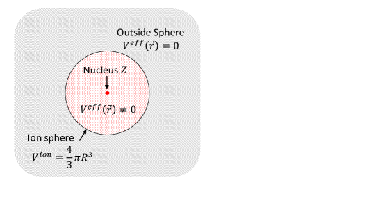
Figure 1: (Color online) Schematic diagram of average atom physical model. Inside the ion sphere the electronic structure is determined with density functional theory. The boundary condition is that outside the sphere the effective electron-nucleus potential is zero.

2.3 Electron density

On applying spherical symmetry to the Dirac equation, $n_{e}(r)$ can be written in terms of orbitals [7, 24]

$$n_{e}(r) = \sum\limits_{i\in B}f(\epsilon_{i},\mu)\frac{2|\kappa_{i}|}{4\pi r^{2}}[P^{2}_{\kappa_{i}}(r,\epsilon_{i})+Q^{2}_{\kappa_{i}}(r,\epsilon_{i})]$$ (8)

$$\!\!\!\!\!\!\!\!\!\!\!\!\!\!\!\!\!\!\!\!+\int_{0}^{\infty}d\epsilon f(\epsilon,\mu)\sum_{\stackrel{{\scriptstyle\kappa=-\infty}}{{\kappa\neq 0}}}^{+\infty}\frac{2|\kappa|}{4\pi r^{2}}[P^{2}_{\kappa}(r,\epsilon)+Q^{2}_{\kappa}(r,\epsilon)]$$

where the sum over $i$ runs over all bound states and $P_{\kappa}(r,\epsilon)$ ($Q_{\kappa}(r,\epsilon)$) is the large (small) component of the radial Dirac equation. $\epsilon$ is the energy minus the rest mass of the electron so that it is directly comparable to the energy appearing in the Schrödinger equation. For the Schrödinger equation the expression for $n_{e}(r)$ reads

$$n_{e}(r) = \sum\limits_{i\in B}f(\epsilon_{i},\mu)\frac{2(2l_{i}+1)}{4\pi r^{2}}[P^{2}_{l_{i}}(r,\epsilon_{i})]$$ (9)

$$+\int\limits_{0}^{\infty}d\epsilon\,f(\epsilon,\mu)\sum\limits_{l=0}^{\infty}\frac{2(2l+1)}{4\pi r^{2}}[P^{2}_{l}(r,\epsilon)]$$

where $P_{l}$ is now the solution to the radial Schrödinger equation. Note that the sum over $\kappa$ in equation (8) can be converted into a sum over orbital angular momentum index $l$ with

$$\sum_{\stackrel{{\scriptstyle\kappa=-\infty}}{{\kappa\neq 0}}}^{+\infty}\to\sum_{l=0}^{\infty}\delta_{\kappa,-l-1}+\sum_{l=1}^{\infty}\delta_{\kappa,l}$$ (10)

where $\delta$ is the Kronecker delta. Using this, and setting the small components $Q_{\kappa}=0$, one recovers the non-relativistic expression (9) from the relativsitic one (8).

In terms of the Green’s function the expression for $n_{e}(r)$ is identical for both the relativistic and non-relativistic cases

$$n_{e}(r)=-\frac{1}{\pi}\Im\int_{-\infty}^{\infty}d\epsilon f(\epsilon,\mu)TrG(r,\epsilon)$$ (11)

Relativistically the Green’s function is given by

$$TrG(r,\epsilon) = -\imath p(1+\frac{\epsilon}{2mc^{2}})2m$$ (12)

$$\!\!\!\!\!\!\!\!\!\!\!\!\!\!\!\!\!\!\!\!\!\!\!\!\!\!\!\!\!\!\!\!\!\!\!\!\!\!\!\!\times\sum_{\stackrel{{\scriptstyle\kappa=-\infty}}{{\kappa\neq 0}}}^{+\infty}\frac{2|\kappa|}{4\pi r^{2}}[P_{\kappa}^{R}(r,\epsilon)P_{\kappa}^{I}(r,\epsilon)+Q_{\kappa}^{R}(r,\epsilon)Q_{\kappa}^{I}(r,\epsilon)]$$

where

$$p=\sqrt{2m\epsilon\left(1+\frac{\epsilon}{2mc^{2}}\right)},$$ (13)

is the magnitude of momentum, $P^{R}$ ($P^{I}$) is the large component, regular (irregular) solution to the radial Dirac equation, and $Q^{R}$ ($Q^{I}$) the corresponding small components (see section 2.4).

Non-relativistically, the trace of the Green’s function becomes

$$TrG(r,\epsilon)=-\imath p2m\sum_{l=0}^{\infty}\frac{2(2l+1)}{4\pi r^{2}}[P_{l}^{R}(r,\epsilon)P_{l}^{I}(r,\epsilon)]$$ (14)

where $P^{R}$ ($P^{I}$) is the regular (irregular) solution to the radial Schrödinger equation, and

$$p=\sqrt{2m\epsilon}.$$ (15)

2.4 Boundary Conditions

The boundary conditions at the sphere are that the wavefunctions must match the solution to the Dirac or Schrödinger equations with $V^{eff}(r)=0$, where both equations reduce to the spherical Bessel equation. Relativistically, for negative energy ( $\epsilon<0$ i.e. the bound states), the radial wavefunctions must match

$$P_{\kappa}(R,\epsilon) = A_{\epsilon,\kappa}R\,\imath^{l}\,h_{l}(pR)$$ (16)

$$Q_{\kappa}(R,\epsilon) = A_{\epsilon,\kappa}R\,\imath^{l}\,\mathrm{Sgn}(\kappa)\sqrt{\frac{\epsilon}{\epsilon+2mc^{2}}}h_{\bar{l}}(pR)$$ (17)

with $h_{l}$ the spherical Hankel function and $\bar{l}=l-\mathrm{Sgn(\kappa)}$, where $\mathrm{Sgn}$ returns the sign of the argument, and $A_{\epsilon,\kappa}$ is a constant of proportionality that is determined by the normalization integral

$$\int_{0}^{\infty}dr[P^{2}_{\kappa_{i}}(r,\epsilon_{i})+Q^{2}_{\kappa_{i}}(r,\epsilon_{i})]=1$$ (18)

It is for this normalization integral that we must assume $V^{eff}(r)=0$ for $r\geq R$. For positive energies

$$\!\!\!\!\!P_{\kappa}(R,\epsilon)\!\!\!\! = \!\!\!\!\sqrt{\frac{p}{\pi\epsilon}}pR\left[\cos\delta_{\kappa}j_{l}(pR)+\sin\delta_{\kappa}\eta_{l}(pR)\right]$$ (19)

$$\!\!\!\!\!Q_{\kappa}(R,\epsilon)\!\!\!\! = \!\!\!\!-\mathrm{Sgn}(\kappa)\sqrt{\frac{\epsilon}{\epsilon+2mc^{2}}}$$ (20)

$$\!\!\!\!\!\!\!\!\!\!\!\!\!\!\!\!\!\times\sqrt{\frac{p}{\pi\epsilon}}pR\left[\cos\delta_{\kappa}j_{\bar{l}}(pR)+\sin\delta_{\kappa}\eta_{\bar{l}}(pR)\right]$$

where $j_{l}$ ($\eta_{l}$) is the spherical Bessel (Neumann) function. $\delta_{\kappa}$ is the energy dependent phase shift. The numerical $P_{\kappa}$ and $Q_{\kappa}$ have arbitary normalization. To recover the correct physical normalization (equations (19) and (20)) they are mutiplied by a constant. This constant and $\delta_{\kappa}$ are determined by requiring the numerical the boundary conditions to be satisfied.

Non-relativistically, for negative energies, we have

$$P_{l}(R,\epsilon) = A_{\epsilon,l}R\,\imath^{l}\,h_{l}(pR)$$ (21)

with $A_{\epsilon,l}$ determined by

$$\int_{0}^{\infty}dr[P^{2}_{l_{i}}(r,\epsilon_{i})]=1$$ (22)

and for positive energies

$$\!\!\!\!\!P_{l}(R,\epsilon) = \sqrt{\frac{2mp}{\pi}}R\left[\cos\delta_{l}j_{l}(pR)+\sin\delta_{l}\eta_{l}(pR)\right]$$ (23)

where $\delta_{l}$ and the normalization constant for the numerical $P_{l}$ are determined by requiring the numerical value of $P_{l}(r)$ and its first derivative with respect to $r$ to satisfy the boundary condition (23) and its derivative.

Relativisitcally, for the regular solutions used to construct the Green’s function (equation (12)), the boundary conditions are

$$\!\!\!\!\!P_{\kappa}^{R}(R,\epsilon) = R\left[j_{l}(pR)-\imath ph_{l}(pR)t_{l}(p)\right]$$ (24)

$$\!\!\!\!\!Q_{\kappa}^{R}(R,\epsilon) = \mathrm{Sgn}(\kappa)\sqrt{\frac{\epsilon}{\epsilon+2mc^{2}}}$$ (25)

$$\times R\left[j_{\bar{l}}(pR)-\imath ph_{\bar{l}}(pR)t_{l}(p)\right]$$

where $t_{l}$ is the energy dependent t-matrix that is determined by matching the numerical solution to this boundary condition. It is worth noting that for real energies $\epsilon$ the phase shifts and the t-matrix are simply related [25]. For the irregular solutions

$$\!\!\!\!\!P_{\kappa}^{I}(R,\epsilon) = Rh_{l}(pR)$$ (26)

$$\!\!\!\!\!Q_{\kappa}^{I}(R,\epsilon) = \mathrm{Sgn}(\kappa)\sqrt{\frac{\epsilon}{\epsilon+2mc^{2}}}Rh_{\bar{l}}(pR)$$ (27)

The boundary conditions for the non-relativistic case are

$$\!\!\!\!\!P_{l}^{R}(R,\epsilon) = R\left[j_{l}(pR)-\imath ph_{l}(pR)t_{l}(p)\right]$$ (28)

$$\!\!\!\!\!P_{l}^{I}(R,\epsilon) = Rh_{l}(pR)$$ (29)

2.5 Density of States

Relativistically the density of states $\chi(\epsilon)$ in terms of orbitals is

$$\!\!\!\!\!\!\!\!\chi(\epsilon) \!\!\!\!\!=\!\!\!\!\! \sum_{i\in B}\delta(\epsilon_{i}-\epsilon)\int_{0}^{R}dr\,2|\kappa_{i}|[P^{2}_{\kappa_{i}}(r,\epsilon_{i})+Q^{2}_{\kappa_{i}}(r,\epsilon_{i})]$$ (30)

$$\!\!\!\!\!\!\!\!+\sum_{\kappa}2|\kappa|\int_{0}^{R}dr\,[P^{2}_{\kappa}(r,\epsilon)+Q^{2}_{\kappa}(r,\epsilon)]\Theta(\epsilon)$$

where $\delta$ is the Dirac delta function, and $\Theta$ is the Heaviside step function. Non-relativistically the density of states is

$$\chi(\epsilon) = \sum_{i\in B}\delta(\epsilon_{i}-\epsilon)\int_{0}^{R}dr\,2(2l_{i}+1)[P^{2}_{l_{i}}(r,\epsilon_{i})]$$ (31)

$$+\sum_{l}2(2l+1)\int_{0}^{R}dr\,[P^{2}_{l}(r,\epsilon)]\Theta(\epsilon)$$

In terms of the Green’s function, the expression is identical for both the relativistic and non-relativistic cases

$$\chi(\epsilon)=-\frac{1}{\pi}\Im\int_{V^{ion}}d^{3}r\,TrG(r,\epsilon)$$ (32)

2.6 Equation of State

The electronic free energy $F$ and internal energy $U$ per atom are

$$F = F^{el}+F^{xc}+F^{ks}$$ (33)

$$U = F^{el}+U^{xc}+U^{k}$$ (34)

$F^{el}$ is the electrostatic contribution

$$F^{el}=\frac{1}{2}\int_{V^{ion}}d^{3}r\left[V^{el}(r)-\frac{Z}{r}\right]n_{e}(r)$$ (35)

$F^{xc}$ ($U^{xc}$) is the exchange and correlation free (internal) energy and $F^{ks}$ is the kinetic and entropic term

$$F^{ks}=U^{k}-TS$$ (36)

where $U^{k}$ is the electron kinetic energy contribution to the internal energy

$$U^{k}=\int_{-\infty}^{\infty}d\epsilon f(\epsilon,\mu)\chi(\epsilon)\epsilon-\int_{V^{ion}}d^{3}rV^{eff}(r)n_{e}({r})$$ (37)

and $S$ is the entropy

$$S = -\int_{-\infty}^{\infty}d\epsilon\chi(\epsilon)$$ (38)

$$\!\!\!\!\!\!\!\!\!\!\!\!\!\!\!\!\!\!\!\!\!\!\!\!\!\!\!\!\times\left[f(\epsilon,\mu)\ln(f(\epsilon,\mu))+(1-f(\epsilon,\mu))\ln(1-f(\epsilon,\mu))\right]$$

The electronic pressure $P$ calculated using the Virial theorem is

$$P=\frac{1}{V^{ion}}\left[\frac{\mathscr{T}+F^{el}}{3}\right]+P^{xc}$$ (39)

where

$$P_{xc}=\frac{1}{V^{ion}}\left[-F^{xc}+\int_{V}d^{3}r\,n_{e}(r)V^{xc}(r)\right]$$ (40)

and $\mathscr{T}$ is

$$\mathscr{T}=2\int_{-\infty}^{\infty}d\epsilon f(\epsilon,\mu)\chi^{A}(\epsilon)\epsilon-2\int_{V^{ion}}d^{3}rV^{eff}(r)n^{A}_{e}({r})$$ (41)

Here the superscript $A$ means the quantity due only to the large component. For the relativistic case this means setting $Q_{\kappa}=0$ in the expressions for the density (8) and density of states (30), and in the Green’s function (12) which is then used in expressions (11) and (32). For the non-relativistic case, there is no small component, so $n_{e}(r)=n_{e}^{A}(r)$ and $\chi(\epsilon)=\chi^{A}(\epsilon)$.

2.7 Summary

In this section we have given formulae that both define the model and can be use to evaluate it numerically. In the following section we present practical strategies for solution of the model over a wide range of densities, temperatures and elements based on these expressions.

3 Numerical Methods

3.1 Numerical Solution of the Schrödinger and Dirac Equations

The radial Dirac equations are

$$(V^{eff}(r)-\epsilon)P_{\kappa}+c(\frac{d}{dr}-\frac{\kappa}{r})Q_{\kappa} \!\!\!\!\!=\!\!\!\!\! 0$$ (42)

$$-c(\frac{d}{dr}+\frac{\kappa}{r})P_{\kappa}+(V^{eff}(r)-\epsilon-2mc^{2})Q_{\kappa} \!\!\!\!\!=\!\!\!\!\! 0$$ (43)

and the radial Schrödinger equation is

$$\frac{d^{2}P_{l}}{dr^{2}}+2\left(\epsilon-V^{eff}(r)-\frac{l(l+1)}{2r^{2}}\right)P_{l}=0$$ (44)

These can be solved numerically with a variety of methods. We recommend using the Adams methods, as explained in detail in reference [26] (also used in [27]). We have used the fifth order formula. This is a predictor-corrector method, but solves the predictor-corrector loop analytically. A robust method for obtaining the necessary four point starting values for outward integration is also presented in [26] and is straightforwardly adapted for the inward integrations. Inward integrations (i.e. from $R$ to $0$) for bound states and the irregular solutions start from the boundary condition values.

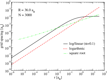
Figure 2: (Color online) Grid spacing $r_{i+1}-r_{i}$ for various grid generation methods described in the text.

For the radial grid we have tried one based on $\sqrt{r}$. A disadvantage is that this does not allow one to vary the total number of grid points $N$ independently from the value of $r$ at the first grid point $r_{1}$. Since the value of $r$ at the end of the grid is fixed by the ion-sphere radius $R$, then $r_{1}=R/N^{2}$. This lack of flexibility is problematic. We have also tried a grid based on $\log r$ [27], which allows such flexibility, but for low densities requires many grid points to maintain resolution near the sphere boundary. Finally, we settled on the log-linear grid presented in [28]. This is logarithmic near the origin and so has enough points to resolve wavefunctions which can vary rapidly for small $r$, and switches to linear spacing as $r$ increases. We have found this grid to be generally accurate from low to high density, and from low $Z$ to high $Z$. We have found $r_{1}=1.0\times 10^{-6}\,a_{B}$ and $N=3000$ to be robust for the applications presented here. The log-linear grid also requires a parameter $\alpha$ to be chosen which determines how quickly it switches from logarithmic to linear. We have found $\alpha=0.1$ to be generally reasonable. Note that $\alpha=0$ corresponds to a purely logarithmic (exponential) grid.

Examples of the grid spacing from these three grid choices are shown in figure 2. For this case (lutetium at 0.01 g/cm³, grid independent of temperatures) we find that $r_{1}$ and the grid spacing for the $\sqrt{r}$ grid are too large for accurate convergence. We also find that the $\log\,r$ grid is too sparse for large $r$. Only the log-linear grid has the resolution everywhere that is needed. Note that we have implemented the Adams method so that Tartarus can use any grid provided that $r$ can be transformed onto a linearly spaced grid $x$ and $dr/dx$ is smooth and can be calculated [26, 27].

3.2 Contour Integrals for Green’s Functions

The main advantage of using the Green’s function is that it is analytic in the complex plane, allowing energy integrals along the real energy axis to be deformed to complex energy $z$ using Cauchy’s integral theorem. The electron density can be calculated thus

$$n_{e}(r) = \frac{1}{\pi}\Im\int_{C}dzf(z,\mu)TrG(r,z)$$ (45)

$$\!\!\!\!\!+2k_{B}T\Re\left\{\sum_{j=1}^{N_{mat}}TrG(r,z_{j})\right\}$$

$C$ refers to a contour that closes when joined to the real axis [1], and the sum over $j$ is a sum over the $N_{mat}$ poles (known as Matsubara poles) of the Fermi-Dirac function enclosed by this closed contour, at energies $z_{j}=\mu+\imath\pi(2j-1)k_{B}T$. Similarly, for equation of state calculation we can use

$$\!\!\!\!\!\int_{-\infty}^{\infty}d\epsilon f(\epsilon,\mu)\chi(\epsilon)\epsilon \!\!\!\!\!=\!\!\!\!\! \!\!\!\frac{1}{\pi}\Im\int_{V^{ion}}\!\!\!\!d^{3}r\!\!\int_{C}dzf(z,\mu)\,z\,TrG(r,z)$$ (46)

$$\!\!\!\!\!\!\!\!\!\!\!\!\!\!\!\!\!\!\!\!\!\!\!\!\!\!\!\!\!\!\!\!\!\!\!\!\!\!\!\!\!\!\!\!\!\!\!\!+2k_{B}T\Re\left\{\int_{V^{ion}}d^{3}r\,\sum_{j=1}^{N_{mat}}\,z_{j}\,TrG(r,z_{j})\right\}$$

The advantage of carrying out the energy integrals in the complex plane is twofold: 1) sharp features in the integrand that occur for real energies are broadened in the complex plane. Hence resonances in the positive energy states that need to be tracked and resolved on the real energy axis are broad and smoothly varying in the complex plane. This point was explored in detail in [1] (also see figure 5), and 2) negative energy (or bound) states are treated in exactly the same way as positive energy states. The search for bound states is tricky to make generally robust, and states with very small energies (eg. $|\epsilon|<1\times 10^{-4}E_{h}$) can be especially hard to accurately represent. By designing the contour $C$ so that it returns to the real axis at a large negative energy, the search for bound states could be avoided altogether. However, since deeply bound states are very sparse in energy space, it makes sense to treat these more deeply bound states with the usual orbital approach, and the more weakly bound states with Green’s functions (see section 3.3).

We have used a rectangular contour, as in reference [1]. To find $\epsilon_{min}$, the energy at which the contour rejoins the real energy axis, we first solve for the bounds states using standard search methods (eg. reference [26]), and look for the highest lying (least negative) energy gap $\geq$ 10 E_h between two states in an energy ordered list. $\epsilon_{min}$ is then set to be 1 E_h less than the eigenenergy of the state on the higher lying side of that gap. This is done at each iteration of the SCF procedure to avoid double counting bound states. It may seem that since we are already finding the bound eigenstates we should just set $\epsilon_{min}=0$ E_h. In many cases this would work, but as mentioned above inaccuracies would occur if our search algorithm missed bound states, or if bound states had very small energies. The Green’s function approach avoids both of these pitfalls and as a result is very stable.

$\epsilon_{max}$ is set by requiring $f(\epsilon_{max},\mu)\approx 10^{-10}$. We split the integration into panels and use a 4 point Gauss-Legrende scheme in each. Care is taken to resolve the Green’s function near the Fermi-edge, which is important for highly degenerate cases, i.e. when $k_{B}\,T/E_{F}<<1$ ($E_{F}$ is the Fermi energy). The total number of points used is dependent on $\epsilon_{min}$, $\epsilon_{max}$ and $\mu$, but typical values are 1000 to 2000 energy points.

While any contour can be used to carry out the energy integrals above, calculation of the entropy is special. Due to the many valued logarithm in (38) the contour cannot pass the branch-cut parallel to the first Matsubara pole at $\Im z=\pi k_{B}T$. For sufficiently high temperature $\pi k_{B}T$ is greater than the imaginary part of the energy anywhere on the contour and so the SCF contour can be used for $S$. Typically this is so for $k_{B}T\gtrsim$ 10 eV. For temperatures less than this we have decided to use a purely orbital based density of states calculation, only for the entropy at the end of the SCF procedure. Hence we use all bound orbitals and a resonance tracker [7] for the positive energy states. Fortunately, at such relatively low temperatures resonance tracking is less challenging and we have found this to be accurate enough for $S$. Note that even for these low $T$ cases Green’s functions are still used in the SCF procedure where we find they offer enhanced stability.

3.3 Density Construction

Electron density $n_{e}(r)$ is the key quantity in density functional theory and must be constructed accurately. While it is in principle possible to construct $n_{e}(r)$ directly from the Green’s function or the orbitals, it is very difficult to do this robustly over a wide range of temperatures or densities and materials. Instead we have used the following numerically advantageous hybrid decomposition

$$\begin{split}n_{e}(r)=&n_{e}^{\scriptscriptstyle core}(r)+n_{e}^{\scriptscriptstyle GF}(r,l_{max})+n_{e}^{\scriptscriptstyle ctm}(r,l_{max})\\ &-n_{e}^{\scriptscriptstyle free}(r,l_{max})+n_{e}^{0}\end{split}$$ (47)

Here $n_{e}^{core}(r)$ is the density due to bound states with $\epsilon<\epsilon_{min}$ (from equation (8))

$$n_{e}^{\scriptscriptstyle core}(r)=\sum\limits_{i\in B,\epsilon_{i}<\epsilon_{min}}f(\epsilon_{i},\mu)\frac{2|\kappa_{i}|}{4\pi r^{2}}[P^{2}_{\kappa_{i}}(r,\epsilon_{i})+Q^{2}_{\kappa_{i}}(r,\epsilon_{i})]$$ (48)

$n_{e}^{\scriptscriptstyle GF}(r,l_{max})$ is calculated using (from equation (11))

$$n_{e}(r)=-\frac{1}{\pi}\Im\int_{\epsilon_{min}}^{\epsilon_{max}}d\epsilon f(\epsilon,\mu)TrG(r,\epsilon,l_{max})$$ (49)

with $TrG(r,\epsilon,l_{max})$ calculated using (from equation (12))

$$TrG(r,\epsilon,l_{max}) = -\imath p(1+\frac{\epsilon}{2mc^{2}})2m$$ (50)

$$\!\!\!\!\!\!\!\!\!\!\!\!\!\!\!\!\!\!\!\!\!\!\!\!\!\!\!\!\!\!\!\!\!\!\!\!\!\!\!\!\!\!\!\!\!\!\!\!\!\!\!\!\!\!\!\!\!\!\!\times\sum_{l=0}^{l_{max}}\sum_{\kappa}\frac{2|\kappa|}{4\pi r^{2}}[P_{\kappa}^{R}(r,\epsilon)P_{\kappa}^{I}(r,\epsilon)+Q_{\kappa}^{R}(r,\epsilon)Q_{\kappa}^{I}(r,\epsilon)]$$

where the sum over $\kappa$ runs over the allowed values of $\kappa$ for a given $l$, i.e. for $l>0$, $\kappa=\{l,-l-1\}$ and for $l=0$, $\kappa=-1$.

$n_{e}^{\scriptscriptstyle ctm}(r,l_{max})$ is the density given by (from equation (8))

$$\begin{split}n_{e}^{\scriptscriptstyle ctm}(r,l_{max})=&\int_{0}^{\epsilon_{max}}d\epsilon f(\epsilon,\mu)\sum_{l=l_{max}+1}^{l_{con}}\sum_{\kappa}\\ &\times\frac{2|\kappa|}{4\pi r^{2}}[P^{2}_{\kappa}(r,\epsilon)+Q^{2}_{\kappa}(r,\epsilon)]\end{split}$$ (51)

$n_{e}^{\scriptscriptstyle free}(r)$ is given by

$$\begin{split}n_{e}^{\scriptscriptstyle free}(r)=&\int_{0}^{\epsilon_{max}}d\epsilon f(\epsilon,\mu)\sum_{l=0}^{l_{con}}\sum_{\kappa}\\ &\times\frac{2|\kappa|}{4\pi r^{2}}[{P^{0}_{\kappa}}^{2}(r,\epsilon)+{Q^{0}_{\kappa}}^{2}(r,\epsilon)]\end{split}$$ (52)

where the superscript $0$ on the orbitals indicates solution to the Dirac equation with $V^{eff}(r)=0$, i.e. the “$free$” solution. $l_{con}$ is determined [5] by incrementing $l$ and evaluating

$$\begin{split}&\int_{0}^{R}dr\,\int_{0}^{\epsilon_{max}}d\epsilon f(\epsilon,\mu)\sum_{\kappa}2|\kappa|\\ &\times\left\{[P^{2}_{\kappa}(r,\epsilon)+Q^{2}_{\kappa}(r,\epsilon)]-[{P^{0}_{\kappa}}^{2}(r,\epsilon)+{Q^{0}_{\kappa}}^{2}(r,\epsilon)]\right\}\\ &<\mbox{{TOL}}\end{split}$$ (53)

until for two consecutive $l$’s this condition is true. We have found TOL $=10^{-4}$ to be robust. $n_{e}^{0}$ is the free electron gas density for temperature $T$ and chemical potential $\mu$. It is used to correct the electron density that has had $n_{e}^{free}(r)$ removed and the $l$ sum truncated at $l_{con}$

$$\begin{split}&n_{e}^{0}=\int_{0}^{\infty}d\epsilon f(\epsilon,\mu)\sum_{l=0}^{\infty}\sum_{\kappa}\frac{2|\kappa|}{4\pi r^{2}}[{P^{0}_{\kappa}}^{2}(r,\epsilon)+{Q^{0}_{\kappa}}^{2}(r,\epsilon)]\\ &=c_{\scriptscriptstyle TF}\left[F_{\frac{1}{2}}(\mu/k_{B}T,k_{B}T/mc^{2})+\frac{k_{B}T}{mc^{2}}F_{\frac{3}{2}}(\mu/k_{B}T,k_{B}T/mc^{2})\right]\end{split}$$ (54)

where $c_{\scriptscriptstyle TF}\equiv\sqrt{2}(k_{B}T)^{\frac{3}{2}}/\pi^{2}$ and

$$F_{n}(\eta,\beta)=\int_{0}^{\infty}dx\frac{x^{n}\sqrt{1+\frac{1}{2}\beta x}}{e^{x-\eta}+1}$$ (55)

are the relativistic Fermi-Dirac integrals [29]. Hence electrons in states with $l>l_{con}$ are treated as free electrons. The convergence of equation (53) ensures that this approximation is accurate.

$l_{max}$ controls which states are treated with Green’s functions, and which are treated with orbitals. Typically we choose $l_{max}\approx 40$, which ensures any resonances in these angular momentum channels are correctly integrated. For $n_{e}^{\scriptscriptstyle ctm}(r)$ and $n_{e}^{\scriptscriptstyle free}(r)$ we use a fixed energy grid, based on a linearly spaced $\sqrt{\epsilon}$ grid and typically use 400 points. Using orbitals on this fixed energy grid is very rapid, more so than the Green’s function evaluation which uses a denser energy grid. Moreover the Green’s function requires both the regular and irregular solutions, whereas the orbital only requires one solution of the Dirac equation. The above decomposition is robust for the cases studied here. The non-relativistic decomposition is identical and can be obtained from the above by setting $Q_{\kappa}=0$, $k_{B}T/mc^{2}=0$ and $\epsilon/2mc^{2}=0$.

This decomposition scheme is also use to evaluate $U^{k}$ and $\mathscr{T}$. Note that, analgous to $n_{e}^{0}$, the free electron gas kinetic energy density $k_{e}^{0}$ is

$$\begin{split}k_{e}^{0}=&\int_{0}^{\infty}d\epsilon f(\epsilon,\mu)\chi^{0}(\epsilon)\epsilon\\ &=c_{\scriptscriptstyle TF}k_{B}T\left[F_{\frac{3}{2}}(\mu/k_{B}T,k_{B}T/mc^{2})\right.\\ &+\left.\frac{k_{B}T}{mc^{2}}F_{\frac{5}{2}}(\mu/k_{B}T,k_{B}T/mc^{2})\right]\end{split}$$ (56)

where $\chi^{0}(\epsilon)$ is the free electron density of states. For $\mathscr{T}$ we have

$$\begin{split}k_{e}^{0,A}=&\int_{0}^{\infty}d\epsilon f(\epsilon,\mu){\chi^{A}}^{0}(\epsilon)\epsilon\\ &=c_{\scriptscriptstyle TF}k_{B}T\left[F_{\frac{3}{2}}(\mu/k_{B}T,k_{B}T/mc^{2})\right]\end{split}$$ (57)

One problem in solving for the Green’s function is that at high $l$ the solution near the origin becomes inaccurate because it results from the multiplication of a very small regular solution and a diverging irregular solution. We have found that this does not present a problem for solution of the SCF problem where small $r$ dependence is suppressed with an $r^{2}$ from the Jabobian. However, for evaluation of the equation of state, integrals like $\int\,d^{3}r\,n_{e}(r)/r$ are required (eg. equation (35)). Hence the result is more sensitive to the small $r$ behavior of $n_{e}(r)$. Thus for equation of state only, we have found it useful to replace $n_{e}(r)$ for $r<10^{-4}$ a_B with an orbital only calculation of the density. Fortunately since we only need the small $r$ part of this density and it is not needed in the SCF calculation, it does not need to be highly accurate. Hence we use a purely orbital based calculation for this part of the density for such integrals only. As for entropy at low temperature, we use all core orbitals and a resonance tracker to replace the Green’s function calculation.

3.4 Self Consistent Field Acceleration

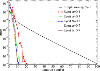
Figure 3: (Color online) Example of SCF acceleration for lutetium at 10 eV and 10 g/cm³. We compare simple mixing to Eyerts method with $M=5$, as a function of the mixing parameter $\alpha$.

Let us denote as $|x\rangle$ a vector generated from $V^{eff}(r)$ or equivalently $n_{e}(r)$, where the components of the vector correspond to the grid points in no particular order. The SCF procedure is

1. Begin with an initial guess of $|x\rangle$.

2. Generate output vector $|x^{out}\rangle$. For example, if $|x\rangle$ is $V^{eff}(r)$ we would solve the Dirac equation, generate $n_{e}(r)$, and then calculate an output potential $V^{eff,out}(r)=|x^{out}\rangle$ by solving the Poisson equation and adding the exchange and correlation potential.

3. Calculate $|F\rangle=|x^{out}\rangle-|x\rangle$.

4. SCF convergence is achieved when $|F\rangle=|0\rangle$. If not achieved, generate new $|x\rangle$ and return to step 2.

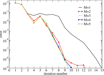
Figure 4: (Color online) Example of SCF acceleration for lutetium at 10 eV and 10 g/cm³. We compare Eyerts method with $\alpha=0.9$ as a function of the order $M$.

In the frequently used simple mixing method the new $|x\rangle$ in step 4 is generated with

$$|x^{(m+1)}\rangle=|x^{(m)}\rangle+\alpha|F^{(m)}\rangle$$ (58)

where $m$ labels the SCF iteration number. $\alpha$ is a mixing parameter that can be adaptive, or fixed. Typically a small value $\alpha=0.1$ is needed for robust convergence and perhaps 80-100 iterations is necessary. A much more robust scheme that greatly reduces the number of iterations required to reach convergence has been given in the work of Eyert [30]. To our knowledge this has not been explored for average atom models before. Eyert’s work is a correction and extension of the more famous Anderson mixing scheme [31]. In this scheme $|x\rangle$ is generated with

$$|x^{(l+1)}\rangle=|x^{(l)}\rangle+\alpha|F^{(l)}\rangle-\sum_{m=l-M}^{l-1}\gamma_{m}^{(l)}\left[|\Delta x^{(m)}\rangle+\alpha|\Delta F^{(m)}\rangle\right]$$ (59)

where $M$ is the order of the mixing (an input choice), the $\gamma_{m}^{(l)}$ are coefficients to be determined, and

$$|\Delta x^{(m)}\rangle = |x^{(m+1)}\rangle-|x^{(m)}\rangle$$ (60)

$$|\Delta F^{(m)}\rangle = |F^{(m+1)}\rangle-|F^{(m)}\rangle$$ (61)

For $M=0$ equation (59) recovers the simple mixing formula above. For $M\geq 1$ we take into account the input and output vectors from the previous $M$ iterations. To find the coefficients $\gamma_{m}^{(l)}$ we solve a matrix equation

$$\underline{\gamma}=\underline{B}^{-1}\underline{A}$$ (62)

where $\underline{\gamma}=[\gamma_{m}^{(l)}]$ is an $M\times 1$ matrix with $m=l-M,\ldots,l-1$, $\underline{A}$ is an $M\times 1$ matrix with elements $\langle\Delta F^{(n)}|F^{(l)}\rangle$ ($n=l-M,\ldots,l-1$). $\underline{B}$ is an $M\times M$ matrix with elements

$$B_{nm}=(1+w_{0}^{2}\delta_{nm})\langle\Delta F^{(n)}|\Delta F^{(m)}\rangle$$ (63)

Note that $\underline{B}$ is a symmetric matrix. Due to saturation of improvements for higher orders, $M$ is taken to be 5 or 6 at maximum [30]. Hence the inversion of the matrix $\underline{B}$ is rapid. $w_{0}^{2}$ is a small parameter that breaks the symmetry (and thus removes linear dependences in Anderson’s original method), it is fixed at $10^{-4}$.

Eyerts method is a quasi-Newton method. It is equivalent to Broyden’s method [32, 33] provided certain choices are made in that method [30]. The mixing parameter $\alpha$ for Eyert’s method can be larger than for simple mixing. In practice we set $|x\rangle=V^{eff}(r)\times r/Z$, and calculate an error using the maximum value of the absolute value of $|F\rangle$. We require error $<10^{-9}$ for two consecutive iterations. In figure 3 we show an example of this, comparing the simple mixing method with the safe choice of $\alpha=0.1$ to Eyert’s method for various $\alpha$. The reduction in number of iterations, even with the same $\alpha$ is remarkable, and results in a corresponding reduction in computational time. Larger values of $\alpha$ lead to improved errors, though the effect saturates by $\alpha=0.9$. It is important to note that not only is Eyert’s method faster but it is also more stable than simple mixing, which can fail to converge in certain cases requiring manual reduction of $\alpha$. Indeed setting $\alpha=0.9$ and running this case with simple mixing the SCF loop fails to converge. In figure 4 we show the effect of the order of Eyert’s method on the error. The advantages saturate by $M=5$. Our default choice in Tartarus is $M=5$, $\alpha=0.9$. We have found this to be very stable, requiring no adjustment for any of the results presented here.

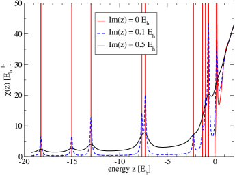
Figure 5: (Color online) Density of states $\chi(z)$ for lutetium at 10 g/cm³ and 10 eV. The solid red line is calculated using orbitals along the real energy axis. Using Green’s functions we can evaluate $\chi(z)$ for complex energy $z$. Increasing the imaginary part of $z$ features, including the discrete bound states and a continuum resonance, are broadened, making them easy to integrate over. Note $\Im{z}=0.5$ E_h is typical for the horizontal part of our integration contour.

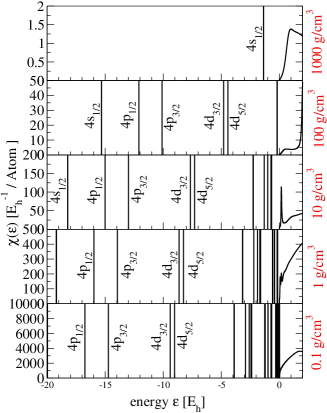
Figure 6: (Color online) Density of states $\chi(\epsilon)$ for lutetium at 10 eV for real energy $\epsilon$.

4 Example

4.1 Density of States

In figure 5 the density of states $\chi(z)$ as a function of complex energy $z$ is shown for lutetium at 10 eV and 10 g/cm³. For $\Im(z)=0$ the calculation is purely in terms of orbitals. We used a bound state search algorithm, and the bound states appear in the figure as vertical lines at negative energies, representing the $\delta(\epsilon_{i}-\epsilon)$. For positive energy states we used a resonance tracker, and a resonance appears at $\sim 0.2$ E_h. For $\Im(z)>0$ the calculation is purely in terms of Green’s functions. We see Lorentzian like line shapes around each bound state energy and around the resonance. For $\Im(z)=0.5$ E_h the features are well smoothed out and integrating over them is accurate and does not need adaptive mesh refinement, as a resonance tracker does. This is the principal advantage of using Green’s functions.

In figure 6 the density of states $\chi(z)$ along the 10 eV isotherm, from $\sim 1/100^{th}$ to 100 times solid density is shown. At the lowest density the most bound states exist (more appear at more negative energies). A few have been labeled in the figure to show that as density increases the bound states move toward the continuum (positive energy) and eventually disappear (pressure ionize). A resonance appears if a state with $l>0$ is nearly bound. On reducing the density this resonance will transition to being a bound state with negative energy. The resonance is a result of the centrifugal barrier term, $-l(l+1)/r^{2}$ in the Schrödinger equation. Hence there are no resonances associated with $l=0$ states.

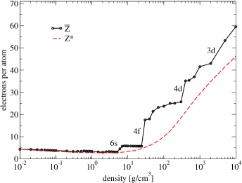
Figure 7: (Color online) Average ionization of lutetium at 10 eV. Two definitions are explored. Note that the definition choice does not affect in any way the properties of the average atom, for example, the equation of state does not depend on the definition. For $\bar{Z}$ the more prominent ionization features are labelled.

4.2 Extraction of Ionization

A quantity of interest is the average ionization in the plasma. This is quantity is not uniquely definable, but given a definition it can be calculated from Tartatus. We stress that the ionization definition has no bearing on the model, it does not influence in any way the results for the self-consistent solution or the equation of state. Here we explore two definitions. The first is the number of positive energy electrons $\bar{Z}$, defined as

$$\!\!\!\!\!\!\!\!\!\!\!\!\!\!\!\!\!\!\!\!\!\!\!\!\!\!\bar{Z} \!\!\!\!\!=\!\!\!\!\! Z-\int_{0}^{R}dr\,\sum\limits_{i\in B}f(\epsilon_{i},\mu)2|\kappa_{i}|[P^{2}_{\kappa_{i}}(r,\epsilon_{i})+Q^{2}_{\kappa_{i}}(r,\epsilon_{i})]$$ (64)

$$\!\!\!\!\!\!\!\!\!\!\!\!\!\!\!\!\!\!\!\!=\int_{0}^{R}dr\,\int_{0}^{\infty}d\epsilon f(\epsilon,\mu)\sum_{\stackrel{{\scriptstyle\kappa=-\infty}}{{\kappa\neq 0}}}^{+\infty}2|\kappa|[P^{2}_{\kappa}(r,\epsilon)+Q^{2}_{\kappa}(r,\epsilon)]$$

The second definition is the number of free electrons per atom $Z^{*}$, i.e. given $\mu$, $T$ and $V^{ion}$, the number of electrons per atom in a free electron gas. This is given by $Z^{*}=n_{e}^{0}V^{ion}$, where $n_{e}^{0}$ is given by equation (54). The first definition $\bar{Z}$ has the benefit that it gives the expected ionization in seemingly clear cut cases: for example $\bar{Z}=3$ for aluminum under normal conditions. However it has the major disadvantage that it is generally discontinuous across a pressure ionization. When a state is ionized it ceases to be included in the bound state sum, and instantly is counted in $\bar{Z}$. In reality the ionized state retains some of its bound like character if it appears as a resonance. These meta-stable resonance states are treated as fully ionized in the $\bar{Z}$ definition. In figure 7 such discontinuities are observed for a lutetium 10 eV isotherm.

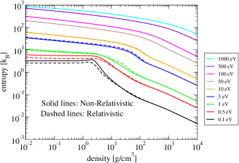
Figure 8: (Color online) Isotherms of entropy of lutetium plasma from Tartarus. Both non-relativistic (solid lines) and relativistic (dashed lines) are shown for temperatures from 0.1 eV to 1 keV. For any given density the entropy increases with temperature, as expected.

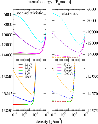
Figure 9: (Color online) Isotherms of internal energy of lutetium plasmas from Tartarus. Both non-relativistic (solid lines) and relativistic (dashed lines) are shown for temperatures from 0.1 eV to 1 keV.

The second definition does not recover the expected ionization in cases like normal density aluminum, where $Z^{*}\approx 2$. However it is smooth across a pressure ionization because the chemical potential $\mu$ is smooth, as it must be (figure 7). Depending on the application one can choose the definition that best suits. But it is important to keep in mind that the ionization depends on the definition.

5 Case Study: Equation of State of Lutetium

We now focus of an application of Tartarus to the equation of state of a high $Z$ material (lutetium, $Z$ = 71), from 0.1 to 1000 eV and $1/1000^{th}$ to 1000 times solid density ($\approx 10$ g/cm³).

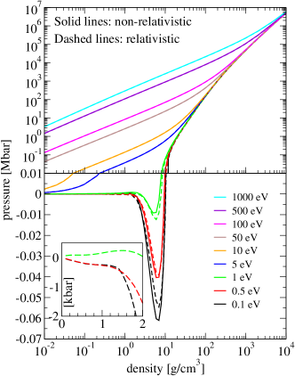
Figure 10: (Color online) Electron pressure of lutetium plasmas along isotherms. Both relativistic and non-relativistic results are shown. The inset also shows electron pressure but focused on the low temperature region where entropy increases with density for fixed temperature. The result is a region where pressure increases as temperature is lowered, for a fixed density.

In figure 8 entropy ($S$) isotherms are shown for both relativistic and non-relativistic calculations. For a given density $S$ increases with temperature, as expected. For $k_{B}T\geq 1$ eV $S$ always decreases as density is increased, again as expected. However for $k_{B}T<1$ eV there is a region near normal density where the model predicts that $S$ increases with density. This physically unexpected behavior is not numerical inaccuracy but a consequence of the physical assumptions of the model [34]. This behaviour is caused by the inconsistency between the normalization integral (18), which is over all space, and the cell neutrality condition (3). When a bound state has significant probability outside the ion sphere, the number of electrons that bound state can contain becomes less that $2(2l+1)$ (non-relativistically). The left-over electrons are forced into the positive energy states leading to an increase in $S$. When the temperature is high enough this effect still occurs but is overwhelmed by the entropy of the other ionized electrons.

The effect of relativity is generally modest, but it does make a significant difference at low temperatures and densities. This is because $S$ is dominated by the density of states near $\epsilon=\mu$ at low temperature. For low densities the splitting of spin degeneracy in the Dirac equation results in the non-relativistic $5p$ state becoming a $5p_{\frac{1}{2}}$ and $5p_{\frac{3}{2}}$, resulting in a change in the eigenvalue and therefore $\mu$. For higher densities, but still at low temperatures, $\mu>0$ and the splitting has a smaller effect since the eigenvalues are continuous.

For internal energy the results are shown in figure 9. There is a significant change in going from non-relativistic to relativistic due to significant relativistic effects on the most tightly bound states. At 0.1 eV, 10 g/cm³ the eigenenergy of the $1s$ state changes from $-2146.4$ E_h to $-2318.8$ E_h. Note that $|\epsilon_{1s}|/mc^{2}\approx 0.12$, so a significant relativistic effect is expected.

In figure 10 the pressure due to electrons (i.e. no ideal ion contribution is added) is shown. In the top panel the relativistic and non-relativistic results are barely distinguishable on the log-log scale. The bottom panel shows the same data but on a linear pressure scale and focused on the low pressure region. Approaching zero temperature at T=0.1 eV, Tartarus gives equilibrium volumes 10.1 g/cm³ in the non-relativistic case and 10.3 g/cm³ in the relativistic case, indicated by zero pressure. This is quite close to the room temperature crystal density of 9.84 g/cc. The negative pressure region is due to treating the material as a continuum, instead of as a mixed phase, such as a liquid-gas coexistence, which the model does not support.

In figure 11 the electron pressure divided by that of a fully ionized ideal electron system is shown. The maximum value that this quantity can take is 1. Even at 10^-2 g/cm³ and 1000 eV the normalized pressure is only $\approx 0.85$. Under these conditions the $1s_{1/2}$ and $2s_{1/2}$ states have eigenvalues of -2514.132 E_h and -575.749 E_h respectively and $\mu=$ -420.128 E_h, so that the Fermi-Dirac occupation factors are 1.000 and 0.986, i.e. nearly completely full. Hence the reduction in pressure from the fully ionized gas.

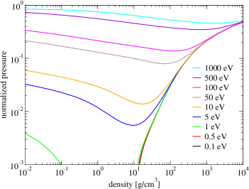
Figure 11: (Color online) Electron pressure for lutetium divided by the pressure of a non-interacting, relativistic, quantum electron gas with electron density $Z/V^{ion}$.

The Maxwell relation

$$\left.\frac{\partial S}{\partial V}\right|_{T}=\left.\frac{\partial P}{\partial T}\right|_{V}$$ (65)

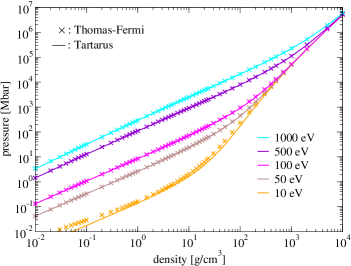
Figure 12: (Color online) Electron pressure for lutetium from Tartarus (relativistic) compared the Thomas-Fermi model’s prediction [35]. Note we have used the same exchange and correlation potential for both [36].

implies that the increase in $S$ with density for low temperatures observed in figure 8 should correspond to a region where the pressure $P$ decreases as temperature increases, at constant density. In the inset in figure 10 such an effect is observed. It is only seen for low temperatures and only over the limited region in which $\left.\frac{\partial S}{\partial V}\right|_{T}$ is negative. Such a behavior is likely to be an artifact of the model. This low temperature metal-to-nonmetal transition region is difficult to model accurately and the present one-atom, spherically symmetric model cannot be expected to fully capture this physics, though it clearly captures the gross effect.

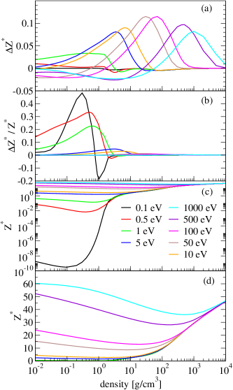
Figure 13: (Color online) The effect of finite temperature exchange and correlation on the average ionization per atom $Z^{*}$. We compare the zero temperature Perdew-Zunger (PZ) functional [36] to the recent finite temperature functional [37] (here labeled QMC17). In the panel (a) we show $\Delta Z^{*}=Z^{*}$(PZ) - $Z^{*}$(QMC17), in panel (b) we show $\Delta Z^{*}/Z^{*}$, where $Z^{*}$ is calculated with PZ. The bottom two panels (c) and (d) show the same $Z^{*}$(PZ) but on different scales.

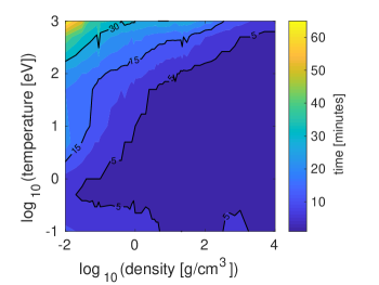
Figure 14: (Color online) Wall-time of Tartarus for the relativistic lutetium cases presented in figures 8 to 13. Contour steps are at 5 minute intervals, and a select few have been labeled explictly.

In figure 11 we also observe a minimum in the normalized pressure. This corresponds to a minimum in ionization $Z^{*}$ (see figure 13). Ionized electrons are the main cause of electronic pressure [5]. The ionization increases with density for high densities due to pressure ionization, a process analogous to the raising of energy levels in a square well potential as the length of the square well is decreased. Bound states disappear with increasing density and there are insufficient bound states to hold all the electrons, so they are forced into positive energy states, i.e. ionized. At low densities, average ionization increases as density is lowered. In this case there are enough electron states to hold all the electrons but their Fermi-Dirac occupation factors become $<$ 1. This arises from the fact that the bound states approach their isolated atom limit, and hence become insensitive to changes in density, however, the chemical potential continues to decrease, leading to smaller Fermi-Dirac occupations factors for the same state. The physical process underlying this is photo ionization. Though there are no radiation fields explicitly included in the model’s Hamiltonian, the assumption of local thermodynamical equilibrium implies that the radiation temperature is equal to the electron temperature. This is embedded in the Fermi-Dirac occupation factor, which does appear explicitly in the model.

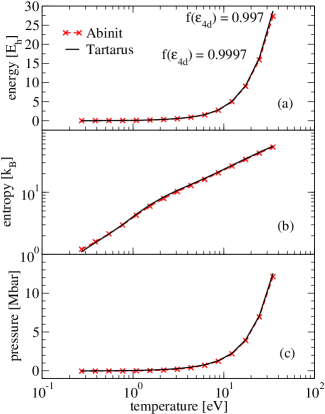
Figure 15: (Color online) Isocore (9.773 g/cm³) of lutetium comparing results from the Abinit plane wave code using a HCP crystal structure to Tartarus results.

In figure 12 we compare the electron pressure from Tartarus to the generalized Thomas-Fermi (TF) model [35], using the same exchange and correlation potential [36]. The TF model is commonly used to construct equation of state tables [38, 39], however it has a number of well known drawbacks. For example, it does not have shell structure and as a consequence its internal energy is quite inaccurate. However it is expected to give the correct pressure at high temperatures and densities. In the figure we observe good agreement of the Tartarus electron pressure with the TF model for high temperatures and densities, in line with this expectation. Note that for truly free electrons the two models become identical. For the lowest temperature in the figure, 10 eV, significant deviations between the models is seen due to the neglect of shell structure in the TF model. The agreement between Tartarus and the TF model is a validation of our implementation in those limits.

All of the results so far presented have used a zero temperature local density approximation (LDA) exchange and correlation functional $F^{xc}$ [36]. Recently, new temperature dependent LDA functionals have become available [40, 37]. This temperature dependence has shown a correction of several percent in the total pressure for some low Z systems in the warm dense matter regime [41]. In figure 13 the effect on $Z^{*}$ of using a temperature dependent $F^{xc}$ is plotted. We have used the functional of Groth et al [37]. The top panel shows the absolute change in $Z^{*}$ (in number of electrons per atom). The effect is generally quite modest, with $|\Delta Z^{*}|\lessapprox 0.1$. In panel (b) the relative change in $Z^{*}$ is plotted. For $k_{B}>50$ eV the effect is $\lessapprox 1$ %. At high temperatures exchange and correlation effects become relatively small, compared to the kinetic energy, as the system becomes more ionized and therefore more like an ideal non-interacting quantum electron gas. At lower temperatures the relative effect of $F^{xc}$ is quite large, approaching 50 % at 0.1 eV. However, in this region the absolute size of $Z^{*}$ is very small (see panels (c) and (d)). The most significant effect is at $\approx 1$ eV and near solid density where both the relative and absolute change in $Z^{*}$ are appreciable. This is sometimes called the warm dense matter regime, and is characterized by significant changes in electronic structure brought about by pressure ionization.

Finally, in figure 14 the wall-time taken to generate the data for figures 8 to 13 is shown. These wall-times are for the relativistic version. The non-relativistic version is roughly a factor of 2 faster. The choice of LDA exchange and correlation potential does not significantly affect the wall-time. We ran Tartarus on an Intel®Xeon®CPU E5-2695 v4 (2.10GHz) with 18 physical cores. 18 instances of the serial code were run and the same time, until all temperature/density cases were exhausted, for a total of 54 density points and 9 temperatures (486 temperature/density points total). From the figure we see a dependence on temperature and density. The longest wall-times occur where the plasma is very weakly degenerate and there is significant ionization (low density, high temperature). This is the regime where the Fermi-Dirac occupation factor has a slowly decaying energy tail, and where electrons in high energy, orbial angular monentum states are weakly, but significantly, affected by the highly charged ion. Algorithmically, the wall-time increases here because $l_{con}$ (section 3.3) is largest in this regime. The majority of temperature/density points take less than five minutes. It is worth noting that any particular point could be made (possibly much) faster by tailoring the algorithm or number of grid or energy points. However, these results were produced without any human interference; the same algorithm and numerical parameters were used everywhere.

We now turn to a comparison with a less approximate method. We have used the plane wave DFT code Abinit [42, 43] for calculations on hcp lutetium. In contrast to the atomic sphere boundary conditions and spherical model potential in Tartarus, periodic boundary conditions and a realistic 3d potential are used in Abinit, which is expected to give more accurate results for the cold energy curve and the low energy electronic spectrum. Our Abinit calculations use the projector augmented wave (PAW) method. The Lu PAW atomic data were generated using the Atompaw code [44]. Our starting point for input parameters is the JTH v1.0 data set [45]. We reduced the PAW sphere radius from 2.5 to 2.0 $a_{B}$ to avoid overlap at the highest compressions considered here. All other radii, such as the pseudo-orbital matching radii and compensation charge shape radius were scaled by 0.8. Atomic states up to $4d$ are treated as part of the frozen core. The LDA exchange correlation functional has been used for comparability with Tartarus. The plane wave cutoff in Abinit was 30 $E_{h}$. Cold energy calculations used “cold smearing” (occopt =4) with smearing parameter 0.01 $E_{h}$ and an $8^{3}$ k-point mesh. High temperature calculations used Fermi-Dirac occupation at the stated temperature with a $4^{3}$ k-point mesh. In the high temperature calculations, the number of bands was set to 540, which results in occupation of the highest band of $\sim 5\times 10^{-4}$ at the highest temperature considered, $T=35$ eV.

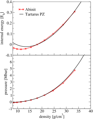
Figure 16: (Color online) Isotherm (0.0285 eV) for lutetium compared to the plane wave code Abinit using the HCP crystal structure.

In constructing wide-range equations of state, an average atom model is often used for the contribution of thermally excited electrons, with the cold energy and pressure subtracted. This allows for an empirical cold curve, or one calculated with a more detailed electronic structure method, to be substituted. In figure 15 we compare the thermal equation of state from Tartarus to Abinit for lutetium at solid density for temperature from $\approx$ 0.25 eV to $\approx$ 25 eV. Overall, there is a remarkable level of agreement between the two methods. For internal energy (panel (a)) some differences appear at the two highest temperature points. For these points we have noted the value of the Fermi-Dirac occupation factor as calculated in Tartarus for the 4d state. Clearly this state is beginning to be temperature ionized, indicating that the frozen core approximation used in the Abinit calculations is near the limit of its validity, and is likely the cause of the difference seen. For entropy (panel (b)) small differences between the models are apparent. It is not surprising that the spherically symmetric average atom model that does not explicitly account for crystal structure fails to exactly reproduce the less approximate plane wave code. Nevertheless, despite these approximations the level of agreement seen is very good. Even at low temperature, where details of the low energy spectrum are important, the two methods differ by well under $1k_{B}$. The structure in the entropy curves at $\sim 2$ eV is well reproduced by Tartarus. For pressure (panel (c)) the agreement is again excellent, with the only significant differences appearing at high temperature, again likely due to the frozen core approximation in Abinit.

In figure 16 we compare Tartarus to Abinit for the cold pressure and energy. The cold EOS is sensitive to details of chemical bonding, and we expect it to be the most challenging for the average atom model. The Tartarus calculation uses an electron temperature of 0.0285 eV, while Abinit uses Fermi surface smearing as described above. In the figure we can see that there are significant differences between the models for internal energy, approaching 0.04 E_h at normal density. Perhaps more importantly is that the trends as a function of density are not well reproduced by the simpler model. It is worth noting that such absolute differences would not be apparent if plotted on the same scale as figure 15. The point being that while tartarus clearly gets large scale trends correct, smaller scale trends may be incorrect.

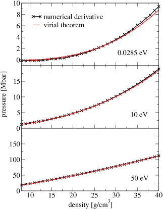
Figure 17: (Color online) Comparison of pressures from Tartarus for lutetium calculated with the Virial expression (39) and via a numerical differentiation of the free energy $P=-\partial F/\partial V|_{T}$.

For pressure, figure 16, the agreement is reasonable on the scale of the figure. The pressure shown is calculated using the Virial expression, equation (39). It is also possible to calculate the pressure by taking a numerical derivative of the free energy $F$

$$P=-\left.\frac{\partial F}{\partial V}\right|_{T}$$ (66)

As is well documented [2, 24], the physical model that Tartarus uses does not guarantee the these two pressures will be identical. In figure 17 we show the pressure calculated both these ways for three isotherms of lutetium. For the cold curve (0.0285 eV) significant differences are observed. By 10 eV the differences are largely gone but show up at the highest densities. At 50 eV the agreement between the two pressures is very good. Generally differences appear where oscillations in the electron density have not died out by the sphere boundary. Such oscillations are a consequence of a sharp Fermi-Dirac distribution which occurs in degenerate systems and are called Friedel oscillations. The figure reflects this: the larges differences are seen for the most degenerate systems (i.e. low temperature and high density).

Such an inherent thermodynamic inconsistency may or may not be problematic depending on the application of the model. A practical solution is to just use the free energy to generate the entire EOS through numerical derivatives. Such an approach generates other problems, principally that the free energy must be smooth enough for the derivatives to be accurate. For many applications however, such inconsistency is not particularly problematic. We note that a thermodynamical consistent average atom is possible [46, 24].

6 Conclusions

We have presented a detailed discussion of the physics model and numerical implementation of the Tartarus average atom code. The model is based on a hybrid orbital and Green’s function implementation and the advantages of such a scheme are presented. A numerically efficient method of solving the self consistent field problem is also given. It is hoped that this presentation may guide others in their own implementations.

We then focus on the application of the model to a lutetium plasma for a wide range of conditions. We use this example to explain concepts such as broadening of the density of states in the complex energy plane, and prediction of ionization. The effect of relativity on the wide ranging EOS is also presented. It is found that relativity is generally a small effect, but is important for internal energy, and for entropy at low temperature and density.

The effect of finite temperature exchange and correlation potentials is also investigated. It is found the effect is generally small, but becomes relatively significant for warm dense matter conditions, i.e. near normal density and temperature around 1 eV.

A comparison of the model to a more physically realistic model at low temperatures reveals the Tartarus model is generally in very good agreement with the more physically accurate model, but that smaller scale deviations are apparent.

Some oddities of the model are discussed. We find that an increase in entropy near normal density along at low temperature isotherm corresponds to a region where pressure decreases as temperature increases, for fixed density. This artifact of the model occurs in a small region, at low temperature where the material is transitioning from metal to non-metal. Also, thermodynamic inconsistency for highly degenerate materials is discussed.

In summary, the hybrid orbital/Green’s function approach to the average atom model was found to be very stable numerically and is recommended for future implementations.

References

- [1] C. E. Starrett. A green’s function quantum average atom model. High Energy Density Phys., 16:18, 2015.
- [2] Nathanael Matthew Gill and Charles Edward Starrett. Tartarus: A relativistic green’s function quantum average atom code. High Energy Density Physics, 24:33–38, 2017.
- [3] David A. Liberman. Self-consistent field model for condensed matter. Phys. Rev. B, 20:4981–4989, Dec 1979.
- [4] David A Liberman. Inferno: A better model of atoms in dense plasmas. Journal of Quantitative Spectroscopy and Radiative Transfer, 27(3):335–339, 1982.
- [5] T. Blenski and K. Ishikawa. Pressure ionization in the spherical ion-cell model of dense plasmas and a pressure formula in the relativistic pauli approximation. Phys. Rev. E, 51:4869, 1995.
- [6] W. R. Johnson, C. Guet, and G. F. Bertsch. Optical properties of plasmas based on an average-atom model. Journal of Quantitative Spectroscopy and Radiative Transfer, 99(1):327–340, 2006.
- [7] B. Wilson, V. Sonnad, P. Sterne, and W. Isaacs. Purgatorio–a new implementation of the inferno algorithm. J. Quant. Spect. Rad. Trans., 99:658, 2006.
- [8] PA Sterne, SB Hansen, BG Wilson, and WA Isaacs. Equation of state, occupation probabilities and conductivities in the average atom purgatorio code. High Energy Density Physics, 3(1-2):278–282, 2007.
- [9] M. Klapisch A. Bar-Shalom, J. Oreg. EOSTA—an improved EOS quantum mechanical model in the sta opacity code. J. Quant. Spect. Rad. Trans., 99:35, 2006.
- [10] R. M. More. Pressure ionization, resonances, and the continuity of bound and free states. Advances in atomic and molecular physics, 21:305, 1985.
- [11] M.B. Trzhaskovskaya and V.K. Nikulin. Atomic structure data based on average-atom model for opacity calculations in astrophysical plasmas. High Energy Density Physics, 26:1 – 7, 2018.
- [12] Michel Pénicaud. An average atom code for warm matter: application to aluminum and uranium. Journal of Physics: Condensed Matter, 21(9):095409, 2009.
- [13] A.A. Ovechkin, P.A. Loboda, and A.L. Falkov. Transport and dielectric properties of dense ionized matter from the average-atom reseos model. High Energy Density Physics, 20:38 – 54, 2016.
- [14] B. F. Rozsnyai. Relativistic hartree-fock-slater calculations for arbitrary temperature and matter density. Phys. Rev. A, 5:1137, 1972.
- [15] Balazs F. Rozsnyai, James R. Albritton, David A. Young, Vijay N. Sonnad, and David A. Liberman. Theory and experiment for ultrahigh pressure shock hugoniots. Physics Letters A, 291(4–5):226 – 231, 2001.
- [16] F. Perrot. Dense simple plasmas as high-temperature liquid simple metals. Phys. Rev. A, 42:4871–4883, Oct 1990.
- [17] MWC Dharma-Wardana and François Perrot. Density-functional theory of hydrogen plasmas. Physical Review A, 26(4):2096, 1982.
- [18] Junzo Chihara. Unified description of metallic and neutral liquids and plasmas. Journal of Physics: Condensed Matter, 3(44):8715, 1991.
- [19] C. E. Starrett and D. Saumon. Electronic and ionic structures of warm and hot dense matter. Phys. Rev. E, 87:013104, Jan 2013.
- [20] N. David Mermin. Thermal properties of the inhomogeneous electron gas. Phys. Rev., 137:A1441–A1443, Mar 1965.
- [21] Walter Kohn and Lu Jeu Sham. Self-consistent equations including exchange and correlation effects. Physical review, 140(4A):A1133, 1965.
- [22] A. K. Rajagopa. Inhomogeneous relativistic electron gas. J. Phys. C, 11:L943, 1978.
- [23] A. H. MacDonald and S. H. Vosko. A relativistic density functional formalism. J. Phys. C, 12:2977, 1979.
- [24] R. Piron and T. Blenski. Variational-average-atom-in-quantum-plasmas (vaaqp) code and virial theorem: Equation-of-state and shock-hugoniot calculations for warm dense al, fe, cu, and pb. Phys. Rev. E, 83:026403, Feb 2011.
- [25] J. Zabloudil, R. Hammerling, L. Szunyogh, and P. Weingberger. Electron Scattering in Solid Matter: a Theoretical and Computational Treatise. Springer Science Business Media, 2000.
- [26] Walter R Johnson. Atomic structure theory. Springer, 2007.
- [27] O. Čertík, J. E. Pask, and J. Vackář. dftatom: A robust and general Schrodinger and Dirac solver for atomic structure calculations. Computer Physics Communications, 184:1777–1791, 2013.
- [28] B.G. Wilson and V. Sonnad. A note on generalized radial mesh generation for plasma electronic structure. High Energy Density Physics, 7(3):161 – 162, 2011.
- [29] Z. Gong, L. Zejda, and W. Dappen. Generalized Fermi-Dirac functions and derivatives: properties and evaluation. Comp. Phys. Commun., 136:294, 2001.
- [30] V. Eyert. A comparative study on methods for convergence acceleration of iterative vector sequences. Journal of Computational Physics, 124(2):271–285, 1996.
- [31] Donald G. Anderson. Iterative procedures for nonlinear integral equations. Journal of the ACM (JACM), 12(4):547–560, 1965.
- [32] Charles G. Broyden. A class of methods for solving nonlinear simultaneous equations. Mathematics of computation, 19(92):577–593, 1965.
- [33] D. D. Johnson. Modified broyden’s method for accelerating convergence in self-consistent calculations. Phys. Rev. B, 38:12807–12813, Dec 1988.
- [34] Philip A. Sterne. From inferno to purgatorio: An average-atom approach to equation of state and electrical conductivity calculation. UCRL-PRES-225592.
- [35] R. P. Feynman, N. Metropolis, and E. Teller. Equations of state of elements based on the generalized fermi-thomas theory. Phys. Rev., 75:1561–1573, May 1949.
- [36] J. P. Perdew and Alex Zunger. Self-interaction correction to density-functional approximations for many-electron systems. Phys. Rev. B, 23:5048–5079, May 1981.
- [37] Simon Groth, Tobias Dornheim, Travis Sjostrom, Fionn D. Malone, W. M. C. Foulkes, and Michael Bonitz. Ab initio exchange-correlation free energy of the uniform electron gas at warm dense matter conditions. Phys. Rev. Lett., 119(13):135001, September 2017.
- [38] S. P. Lyon (ed.) and J. D. Johnson (ed.). Sesame: The los alamos national laboratory equation of state database. Los Alamos National Laboratory Tech. Rep., LA-UR-92-3407, 1992.
- [39] R. M. More, K. H. Warren, D. A. Young, and G. B. Zimmerman. A new quotidian equation of state (qeos) for hot dense matter. The Physics of Fluids, 31(10):3059–3078, 1988.
- [40] Valentin V. Karasiev, Travis Sjostrom, James Dufty, and S. B. Trickey. Accurate homogeneous electron gas exchange-correlation free energy for local spin-density calculations. Physical review letters, 112(7):076403, 2014.
- [41] Travis Sjostrom and Jérôme Daligault. Gradient corrections to the exchange-correlation free energy. Phys. Rev. B, 90:155109, Oct 2014.
- [42] X. Gonze, B. Amadon, P. M. Anglade, J. M. Beuken, F. Bottin, P. Boulanger, F. Bruneval, D. Caliste, R. Caracas, M. Cote, T. Deutsch, L. Genovese, Ph. Ghosez, M. Giantomassi, S. Goedecker, D. R. Hamann, P. Hermet, F. Jollet, G. Jomard, S. Leroux, M. Mancini, S. Mazevet, M. J. T. Oliveira, G. Onida, Y. Pouillon, T. Rangel, G. M. Rignanese, D. Sangalli, R. Shaltaf, M. Torrent, M. J. Verstraete, G. Zerah, and J. W. Zwanziger. Abinit: First-principles approach to material and nanosystem properties. Computer Physics Communications, 180(12):2582–2615, DEC 2009.
- [43] X Gonze, GM Rignanese, M Verstraete, JM Beuken, Y Pouillon, R Caracas, F Jollet, M Torrent, G Zerah, M Mikami, P Ghosez, M Veithen, JY Raty, V Olevano, F Bruneval, L Reining, R Godby, G Onida, DR Hamann, and DC Allan. A brief introduction to the abinit software package. Zeitschrift Fur Kristallographie, 220(5-6):558–562, 2005.
- [44] N.A.W. Holzwarth, A.R. Tackett, and G.E. Matthews. A projector augmented wave (paw) code for electronic structure calculations, part i: atompaw for generating atom-centered functions. Computer Physics Communications, 135(3):329 – 347, 2001.
- [45] Francçois Jollet, Marc Torrent, and Natalie Holzwarth. Generation of projector augmented-wave atomic data: A 71 element validated table in the xml format. Computer Physics Communications, 185(4):1246 – 1254, 2014.
- [46] T. Blenski and B. Cichocki. Variational theory of average-atom and superconfigurations in quantum plasmas. Phys. Rev. E, 75:056402, 2007.