Evolution of states of an infinite fission-death system

Abstract.

The evolution of an infinite system of interacting point entities with traits $x\in\mathds{R}^{d}$ is studied. The elementary acts of the evolution are state-dependent death of an entity with rate that includes a competition term and independent fission in the course of which an entity gives birth to two new entities and simultaneously disappears. The states of the system are probability measures on the corresponding configuration space and the main result of the paper is the construction of the evolution $\mu_{0}\to\mu_{t}$, $t>0$, of states in the class of sub-Poissonian measures.

1. Introduction

1.1. Posing

In recent years, there has been a lot of studies of the stochastic dynamics of structured populations, see, e.g., [2, 4, 5, 8, 9, 12]. Typically, the structure is introduced by assigning to each entity a trait $x\in X$. Then the population dynamics consists in changing the traits of its members that includes also their appearance and disappearance. Usually, one endows the trait space $X$ with a locally-compact topology and assumes that: (a) the populations are locally finite, i.e., compact subsets of $X$ may contain traits of finite sub-populations only; (b) the dynamics of a given entity is mostly affected by the interaction with entities whose traits belong to a compact neighborhood of its own trait. Then the local structure of the population is determined by the network of such interactions. Since the traits of a finite population lie in a compact subset of $X$, each of its members has a compact neighborhood containing the traits of the rest of population. In view of this, in order to clear distinguish between global and local effects one should deal with infinite populations and noncompact trait spaces. In the statistical mechanics of interacting physical particles, this conclusion had led to the concept of the thermodynamic (infinite-volume) limit, see, e.g., [15, pp. 5,6], and, thereby, to the description of the states of thermal equilibrium as probability measures on the space of particle configurations. Such states are constructed from local conditional states and are Gibbsian, i.e., they satisfy a specific consistency condition.

In this article, we study the Markov evolution of a possibly infinite system of point entities (particles) with trait space $X=\mathds{R}^{d}$, $d\geq 1$. The pure states of the system are locally finite configurations $\gamma\subset\mathds{R}^{d}$, see, e.g., [3, 9, 11, 12], whereas the general states are probability measures on the space of all such configurations. The elementary acts of the evolution are: (a) state-dependent disappearance (death) with rate $m(x)+\sum_{y\in\gamma\setminus x}a(x-y)$; (b) independent fission with rate $b(x|y_{1},y_{2})$ in the course of which the particle with trait $x\in\gamma$ gives birth to two particles, with traits $y_{1},y_{2}\in\mathds{R}^{d}$, and simultaneously disappears from $\gamma$. The model with this kind of death and budding instead of fission, cf. [5], is known as the Bolker-Pacala model. Its recent study can be found in [9, 11], see also the literature quoted therein. A similar model with fission (fragmentation) in which each particle produces a (random) finite number of new particles was introduced and studied in [16]. The main result of the present work is the construction of the global in time evolution of states in a certain class of probability measures.

1.2. The overview

As mentioned above, the state space of the model is the set $\Gamma$ of all subsets $\gamma\subset\mathds{R}^{d}$ such that the set $\gamma_{\Lambda}:=\gamma\cap\Lambda$ is finite whenever $\Lambda\subset\mathds{R}^{d}$ is compact. For compact $\Lambda$, we define the map $\Gamma\ni\gamma\mapsto N_{\Lambda}(\gamma)=|\gamma_{\Lambda}|\in\mathds{N}_{0}$, where $|\cdot|$ denotes cardinality and $\mathds{N}_{0}$ stands for the set of nonnegative integers. Then $\mathcal{B}(\Gamma)$ will denote the smallest $\sigma$-field of subsets of $\Gamma$ with respect to which all these maps are measurable. That is, $\mathcal{B}(\Gamma)$ is generated by the family of sets

$$\Gamma^{\Lambda,n}:=\{\gamma\in\Gamma:N_{\Lambda}(\gamma)=n\},\qquad n\in\mathds{N}_{0},\ \ \Lambda-{\rm compact}.$$ (1.1)

It is known [9, 12] that $(\Gamma,\mathcal{B}(\Gamma))$ is a standard Borel space. The set of $n$-point configurations $\Gamma^{n}$ and the set of all finite configurations $\Gamma_{0}$ then are

$$\Gamma^{n}=\{\gamma\in\Gamma:|\gamma|=n\},\qquad\Gamma_{0}:=\bigcup_{n=0}^{\infty}\Gamma^{n}\in\mathcal{B}(\Gamma).$$

For compact $\Lambda$, we let $\Gamma_{\Lambda}=\{\gamma:\gamma\subset\Lambda\}\subset\Gamma_{0}$ and define

$$\mathcal{B}(\Gamma_{\Lambda})=\{\mathbb{A}\cap\Gamma_{\Lambda}:\mathbb{A}\in\mathcal{B}(\Gamma)\}\subset\mathcal{B}(\Gamma_{0})=\{\mathbb{A}\cap\Gamma_{0}:\mathbb{A}\in\mathcal{B}(\Gamma)\}\subset\mathcal{B}(\Gamma).$$

Clearly, $(\Gamma_{0},\mathcal{B}(\Gamma_{0}))$ and $(\Gamma_{\Lambda},\mathcal{B}(\Gamma_{\Lambda}))$ are standard Borel spaces. By $\mathcal{P}(\Gamma)$, $\mathcal{P}(\Gamma_{0})$, $\mathcal{P}(\Gamma_{\Lambda})$ we denote the sets of all probability measures on $(\Gamma,\mathcal{B}(\Gamma))$, $(\Gamma_{0},\mathcal{B}(\Gamma_{0}))$ and $(\Gamma_{\Lambda},\mathcal{B}(\Gamma_{\Lambda}))$, respectively.

For a compact $\Lambda$ and $\mathbb{A}\in\mathcal{B}(\Gamma_{\Lambda})$, we set $\mathbb{C}_{\mathbb{A}}=\{\gamma\in\Gamma:\gamma_{\Lambda}\in\mathbb{A}\}$ and let $\mathcal{B}_{\Lambda}(\Gamma)$ be the sub-$\sigma$-field of $\mathcal{B}(\Gamma)$ generated by all such cylinder sets $\mathbb{C}_{\mathbb{A}}$. A cylinder function $F:\Gamma\to\mathds{R}$ is a $\mathcal{B}_{\Lambda}(\Gamma)/\mathcal{B}(\mathds{R})$-measurable function for some compact $\Lambda$. Here by $\mathcal{B}(\mathds{R})$ we denote the Borel $\sigma$-field of subsets of $\mathds{R}$. For a compact $\Lambda$ and a given $\mu\in\mathcal{P}(\Gamma)$, by setting

$$\mu(\mathbb{C}_{\mathbb{A}})=\mu^{\Lambda}(\mathbb{A})$$ (1.2)

we determine $\mu^{\Lambda}\in\mathcal{P}(\Gamma_{\Lambda})$ – the projection of $\mu$. Note that all such projections $\{\mu^{\Lambda}\}_{\Lambda}$ of a given $\mu\in\mathcal{P}(\Gamma)$ are consistent in the Kolmogorov sense.

Each $\mu\in\mathcal{P}(\Gamma)$ is characterized by its values on the sets (1.1); in particular, by their local moments

$$\int_{\Gamma}N_{\Lambda}^{m}d\mu=:\mu(N_{\Lambda}^{m})=\sum_{n=0}^{\infty}n^{m}\mu(\Gamma^{\Lambda,n}),\qquad m\in\mathds{N}.$$ (1.3)

This characterization naturally includes the dependence of $\mu(\Gamma^{\Lambda,n})$ on $n$. A homogeneous Poisson measure $\pi_{\varkappa}\in\mathcal{P}(\Gamma)$ with density $\varkappa>0$ has the property $\pi_{\varkappa}(\Gamma_{0})=0$. For this measure, it follows that

$$\pi_{\varkappa}(\Gamma^{\Lambda,n})=\frac{\left(\varkappa|\Lambda|\right)^{n}}{n!}\exp\left(-\varkappa|\Lambda|\right),$$ (1.4)

where $|\Lambda|$ stands for the volume of $\Lambda$. In our consideration, the set of sub-Poissonian measures $\mathcal{P}_{\rm exp}(\Gamma)$ plays an important role, see Definition 2.1 below and the corresponding discussion in [9, 11]. For each $\mu\in\mathcal{P}_{\rm exp}(\Gamma)$, there exists $\varkappa>0$ such that

$$\mu(N_{\Lambda}^{m})\leq\pi_{\varkappa}(N_{\Lambda}^{m}),$$ (1.5)

holding for all compact $\Lambda$ and $m\in\mathds{N}$.

The Markov evolution is described by the Kolmogorov equation

$$\dot{F}_{t}=LF_{t},\qquad F_{t}|_{t=0}=F_{0},$$ (1.6)

where $\dot{F}_{t}$ denotes the time derivative of an observable $F_{t}:\Gamma\to\mathds{R}$. The operator $L$ determines the model, and in our case it is

$$(LF)(\gamma)=\sum_{x\in\gamma}\left(m(x)+\sum_{y\in\gamma\setminus x}a(x-y)\right)\left[F(\gamma\setminus x)-F(\gamma)\right]$$ (1.7)

$$+\sum_{x\in\gamma}\int_{(\mathds{R}^{d})^{2}}b(x|y_{1},y_{2})\left[F(\gamma\setminus x\cup\{y_{1},y_{2}\})-F(\gamma)\right]dy_{1}dy_{2}.$$

In expressions like $\gamma\cup x$, we treat $x$ as the singleton $\{x\}$. The first term in (1.7) describes the death of the particle with trait $x$ occurring: (i) independently with rate $m(x)\geq 0$; (ii) under the influence (competition) of the rest of the particles in $\gamma$ occurring with rate

$$E^{a}(x,\gamma\setminus x):=\sum_{y\in\gamma\setminus x}a(x-y)\geq 0.$$ (1.8)

The second term in (1.7) describes independent fission with rate $b(x|y_{1},y_{2})\geq 0$.

The evolution of states $\mu_{0}\to\mu_{t}$ is defined by the Fokker-Planck equation

$$\dot{\mu}_{t}=L^{*}\mu_{t},\qquad\mu_{t}|_{t=0}=\mu_{0},$$ (1.9)

where $L^{*}$ is related to (1.7) according to the rule $(L^{*}\mu)(\mathbb{A})=\mu(L\mathds{1}_{\mathbb{A}})$, $\mathbb{A}\in\mathcal{B}(\Gamma)$; $\mathds{1}_{\mathbb{A}}$ is the indicator function. Both evolutions are in the duality $\mu_{0}(F_{t})=\mu_{t}(F_{0})$. Here and in the sequel, we use the notation $\mu(F)=\int Fd\mu$, cf. (1.3).

The direct use of $L$ and/or $L^{*}$ as linear operators in appropriate Banach spaces is possible only if one restricts the consideration to states on $\Gamma_{0}$. Otherwise, the sums in (1.7) and (1.8) – taken over infinite configurations – may not exist. At the same time, constructing evolutions of finite sub-populations contained in compact sets followed by taking the ‘infinite-volume’ limit – as it is done in the theory of Gibbs fields [15] – can hardly be realized here as the evolution usually destroys the consistency of the local states. Instead of trying to construct global states from local ones, we will we proceed as follows. Let $C_{0}(\mathds{R}^{d})$ stand for the set of continuous real-valued functions with compact support. Then the map

$$\Gamma\ni\gamma\mapsto F^{\theta}(\gamma):=\prod_{x\in\gamma}(1+\theta(x)),\qquad\theta\in\varTheta:=\{\theta\in C_{0}(\mathds{R}^{d}):\theta(x)\in(-1,0]\},$$

is clearly measurable and satisfies $0<F^{\theta}(\gamma)\leq 1$ for all $\gamma$. The set $\varTheta$ clearly has the following properties: (a) for each pair of distinct $\gamma,\gamma^{\prime}\in\Gamma$, there exists $\theta\in\varTheta$ such that $F^{\theta}(\gamma)\neq F^{\theta}(\gamma^{\prime})$; (b) for each pair $\theta,\theta^{\prime}\in\varTheta$, the point-wise combination $\theta+\theta^{\prime}+\theta\theta^{\prime}$ is also in $\varTheta$; (c) the zero function belongs to $\varTheta$. From this it follows that $\{F^{\theta}:\theta\in\varTheta\}$ is a measure defining class, i.e., $\mu(F^{\theta})=\nu(F^{\theta})$, holding for all $\theta\in\varTheta$, implies $\mu=\nu$ for each $\mu,\nu\in\mathcal{P}(\Gamma)$, see [1, Proposition 1.3.28, page 113]. Noteworthy, for each $\theta\in\varTheta$, $\mu(F^{\theta})=\mu^{\Lambda_{\theta}}(F^{\theta})$, where a compact $\Lambda_{\theta}$ is such that $\theta(x)=0$ for $x\in\Lambda^{c}_{\theta}:=\mathds{R}^{d}\setminus\Lambda_{\theta}$.

Our results related to (1.7), (1.9) consist in the following:

• Constructing the evolution $[0,+\infty)\ni t\mapsto\mu_{t}\in\mathcal{P}(\Gamma_{0})$, $\mu_{t}|_{t=0}=\mu_{0}\in\mathcal{P}(\Gamma_{0})$, by proving the existence of a unique classical solution of (1.9) in the Banach space $\mathcal{M}$ of signed measures on $\Gamma_{0}$ with bounded variation.

• Constructing the evolution $[0,+\infty)\ni t\mapsto\mu_{t}\in\mathcal{P}_{\rm exp}(\Gamma)$, $\mu_{t}|_{t=0}=\mu_{0}\in\mathcal{P}_{\rm exp}(\Gamma)$, such that:

  • for each compact $\Lambda$ and $t\geq 0$, $\mu_{t}^{\Lambda}$ – as a measure on $\Gamma_{0}$ – lies in the domain $\mathcal{D}(L^{*})\subset\mathcal{M}$;

  • for each $\theta\in\varTheta$, the map $(0,+\infty)\ni t\mapsto\mu_{t}(F^{\theta})$ is continuously differentiable and the following holds

    $$\frac{d}{dt}\mu_{t}(F^{\theta})=(L^{*}\mu^{\Lambda_{\theta}}_{t})(F^{\theta}).$$ (1.10)

Item 1 is realized in Theorem 3.1. The main idea of how to construct the evolution $\mu_{0}\to\mu_{t}$ stated in item 2 is to obtain it from the evolution $B_{0}(\theta)\to B_{t}(\theta)$, $\theta\in\varTheta$ by solving the evolution equation related to those in (1.6) and (1.9). Here $B_{0}(\theta)=\mu_{0}(F^{\theta})$ with $\mu_{0}\in\mathcal{P}_{\rm exp}(\Gamma)$. This is realized in Theorem 4.1 and Corollary 4.2. One of the hardest points of this scheme is to prove that $B_{t}(\theta)=\mu_{t}(F^{\theta})$ for a unique sub-Poissonian measure. At this stage, we deal with the evolution of local states constructed in realizing item 1.

2. Preliminaries and the Model

We begin by briefly introducing the relevant aspects of the technique used in this work. Its more detailed description (including the notations) can be found in [9, 12] and in the publications quoted therein.

2.1. Measures and functions on configuration spaces

It is know that

$$B_{\pi_{\varkappa}}(\theta):=\pi_{\varkappa}(F^{\theta})=\exp\left(\varkappa\int_{\mathds{R}^{d}}\theta(x)dx\right).$$

Obviously, $B_{\pi_{\varkappa}}$ can be continued to an exponential type entire function of $\theta\in L^{1}(\mathds{R}^{d})$.

Definition 2.1.

The set of sub-Poissonian measures $\mathcal{P}_{\rm exp}(\Gamma)$ consists of all those $\mu\in\mathcal{P}(\Gamma)$ for each of which $\mu(F^{\theta})$ can be continued to an exponential type entire function of $\theta\in L^{1}(\mathds{R}^{d})$.

It can be shown that $\mu\in\mathcal{P}_{\rm exp}(\Gamma)$ if and only if $\mu(F^{\theta})$ might be written in the form

$$\mu(F^{\theta})=1+\sum_{n=1}^{\infty}\frac{1}{n!}\int_{(\mathds{R}^{d})^{n}}k^{(n)}_{\mu}(x_{1},\dots,x_{n})\theta(x_{1})\cdots\theta(x_{n})dx_{1}\cdots dx_{n},$$ (2.1)

where $k^{(n)}_{\mu}$ is the $n$-th order correlation function of $\mu$. Each $k^{(n)}_{\mu}$ is a symmetric element of $L^{\infty}((\mathds{R}^{d})^{n})$, and the collection $\{k^{(n)}_{\mu}\}_{n\in\mathds{N}}$ satisfies

$$\|k^{(n)}_{\mu}\|_{L^{\infty}((\mathds{R}^{d})^{n}}\leq\varkappa^{n},\qquad n\in\mathds{N},$$ (2.2)

holding with some $\varkappa>0$. Note that $k^{(n)}_{\mu}$ is positive and $k^{(n)}_{\pi_{\varkappa}}=\varkappa^{n}$; hence, (2.2) means that $k^{(n)}_{\mu}(x_{1},\dots,x_{n})\leq\varkappa^{n}$ by which one gets (1.5).

Now we turn to functions $G:\Gamma_{0}\to\mathds{R}$. It can be proved that such a function is $\mathcal{B}(\Gamma_{0})/\mathcal{B}(\mathds{R})$-measurable if and only if there exists the collection of symmetric Borel functions $G^{(n)}:(\mathds{R}^{d})^{n}\to\mathds{R}$, $n\in\mathds{N}$, such that

$$G(\eta)=G^{(n)}(x_{1},\dots,x_{n}),\qquad{\rm for}\ \ \eta=\{x_{1},\dots,x_{n}\}.$$ (2.3)

Definition 2.2.

A measurable function $G:\Gamma_{0}\to\mathds{R}$ is said to have bounded support if: (a) there exists compact $\Lambda\subset\mathds{R}^{d}$ such that $G(\eta)=0$ whenever $\eta\cap\Lambda\neq\eta$; (b) there exists $N\in\mathds{N}$ such that $G(\eta)=0$ whenever $|\eta|>N$. By $B_{\rm bs}(\Gamma_{0})$ we denote the set of all bounded functions with bounded support. For each $G\in B_{\rm bs}(\Gamma_{0})$, by $\Lambda_{G}$ and $N_{G}$ we denote the smallest $\Lambda$ and $N$ with the properties just mentioned, and use the notations $C_{G}=\sup_{\eta\in\Gamma_{0}}|G(\eta)|$.

The Lebesgue-Poisson measure $\lambda$ on $(\Gamma_{0},\mathcal{B}(\Gamma_{0}))$ is defined by the integrals

$$\int_{\Gamma_{0}}G(\eta)\lambda(d\eta)=G(\varnothing)+\sum_{n=1}^{\infty}\frac{1}{n!}\int_{(\mathds{R}^{d})^{n}}G^{(n)}(x_{1},\dots x_{n})dx_{1}\cdots dx_{n},$$ (2.4)

with all $G\in B_{\rm bs}(\Gamma_{0})$. For such $G$, we set

$$(KG)(\gamma)=\sum_{\eta\Subset\gamma}G(\eta),\qquad\gamma\in\Gamma,$$ (2.5)

where $\eta\Subset\gamma$ means that $\eta\subset\gamma$ and $\eta\in\Gamma_{0}$. Clearly, cf. Definition 2.2, we have that

$$|(KG)(\gamma)|\leq C_{G}\left(1+|\gamma\cap\Lambda_{G}|\right)^{N_{G}},\qquad G\in B_{\rm bs}(\Gamma_{0}).$$ (2.6)

Like in (2.3), we introduce the function $k_{\mu}:\Gamma_{0}\to\mathds{R}$ such that $k_{\mu}(\eta)=k^{(n)}_{\mu}(x_{1},\dots,x_{n})$ for $\eta=\{x_{1},\dots,x_{n}\}$, $n\in\mathds{N}$, and $k_{\mu}(\varnothing)=1$. Then we rewrite (2.1) as follows

$$\mu(F^{\theta})=\int_{\Gamma_{0}}k_{\mu}(\eta)e(\theta;\eta)\lambda(d\eta),\qquad e(\theta;\eta):=\prod_{x\in\eta}\theta(x).$$ (2.7)

For $\mu\in\mathcal{P}_{\rm exp}(\Gamma)$ and a compact $\Lambda$, let $\mu^{\Lambda}$ be the corresponding projection. It is possible to show that $\mu^{\Lambda}$, as a measure on $(\Gamma_{\Lambda},\mathcal{B}(\Gamma_{\Lambda}))$, is absolutely continuous with respect to the Lebesgue-Poisson measure $\lambda$. Hence, we may write

$$\mu^{\Lambda}(d\eta)=R^{\Lambda}_{\mu}(\eta)\lambda(d\eta),\qquad\eta\in\Gamma_{\Lambda}.$$ (2.8)

For each compact $\Lambda$, the Radon-Nikodym derivative $R^{\Lambda}_{\mu}$ and the correlation function $k_{\mu}$ satisfy

$$k_{\mu}(\eta)=\int_{\Gamma_{\Lambda}}R^{\Lambda}_{\mu}(\eta\cup\xi)\lambda(d\xi),\qquad\eta\in\Gamma_{\Lambda}.$$ (2.9)

For each $G\in B_{\rm bs}(\Gamma_{0})$ and $k:\Gamma_{0}\to\mathds{R}$ such that $k^{(n)}\in L^{\infty}((\mathds{R}^{d})^{n})$ the integral

$$\langle\!\langle G,k\rangle\!\rangle:=\int_{\Gamma_{0}}G(\eta)k(\eta)\lambda(d\eta)$$ (2.10)

surely exists. By (2.1), (2.5), (2.8) and (2.10) we then obtain

$$\int_{\Gamma}\left(KG\right)(\gamma)\mu(d\gamma)=\langle\!\langle G,k_{\mu}\rangle\!\rangle$$ (2.11)

holding for all $G\in B_{\rm bs}(\Gamma_{0})$ and $\mu\in\mathcal{P}_{\rm exp}(\Gamma)$. Set

$$B_{\rm bs}^{\star}(\Gamma_{0})=\{G\in B_{\rm bs}(\Gamma_{0}):\left(KG\right)(\gamma)\geq 0\ \ {\rm for}\ \ {\rm all}\ \ \gamma\in\Gamma\}.$$ (2.12)

By [13, Theorems 6.1, 6.2 and Remark 6.3] we know that the following is true.

Proposition 2.3.

Let a measurable function $k:\Gamma_{0}\to\mathds{R}$ have the following properties:

$$(a) \ \ \langle\!\langle G,k_{\mu}\rangle\!\rangle\geq 0,\qquad{\rm for}\ \ {\rm all}\ \ G\in B_{\rm bs}^{\star}(\Gamma_{0});$$

$$(b) \ \ k(\varnothing)=1;$$

$$(c) \ \ k(\eta)\leq C^{|\eta|},\qquad{\rm for}\ \ {\rm some}\ \ C>0.$$

Then there exists a unique $\mu\in\mathcal{P}_{\rm exp}(\Gamma)$ such that $k$ is its correlation function.

Throughout the paper we use the following easy to check identities holding for appropriate functions $g:\mathds{R}^{d}\to\mathds{R}$ and $G:\Gamma_{0}\to\mathds{R}$:

$$\forall x\in\gamma\qquad\sum_{\eta\Subset\gamma}\prod_{z\in\eta}g(z)=(1+g(x))\sum_{\eta\Subset\gamma\setminus x}\prod_{z\in\eta}g(z),$$ (2.13)

$$\int_{\Gamma_{0}}\sum_{\xi\subset\eta}G(\xi,\eta,\eta\setminus\xi)\lambda(d\eta)=\int_{\Gamma_{0}}\int_{\Gamma_{0}}G(\xi,\eta\cup\xi,\eta)\lambda(d\xi)\lambda(d\eta).$$ (2.14)

2.2. The model

As mentioned above, the model which we consider in this work is described by the generator given in (1.7). Its entries are subject to the following

Assumption 1.

The nonnegative measurable $a$, $b$ and $m$ satisfy:

• $a$ is integrable and bounded; hence, we may set

  $$\sup_{x\in\mathds{R}^{d}}a(x)=a^{*},\qquad\int_{\mathds{R}^{d}}a(x)dx=\langle a\rangle.$$

• There exist positive $r$ and $a_{*}$ such that $a(x)\geq a_{*}$ whenever $|x|\leq r$.

• For each $x\in\mathds{R}^{d}$, $b(x|y_{1},y_{2})dy_{1}dy_{2}$ is a symmetric finite measure on $(\mathds{R}^{d})^{2}$; hence, we may set

  $$\langle b\rangle=\int_{(\mathds{R}^{d})^{2}}b(x|y_{1},y_{2})dy_{1}dy_{2},$$

  where, for simplicity, we consider the translation invariant case. The mentioned symmetry means that $b(x|y_{1},y_{2})=b(x|y_{2},y_{1})$.

• The function

  $$\beta(y_{1}-y_{2})=\int_{\mathds{R}^{d}}b(x|y_{1},y_{2})dx$$

  is supposed to be such that $\sup_{x\in\mathds{R}^{d}}\beta(x)=:\beta^{*}<\infty$. By the translation invariance it follows that

  $$\int_{\mathds{R}^{d}}\beta(x)dx=\langle b\rangle.$$

Noteworthy, we do not exclude the case where $b$ is a distribution. For instance, by setting

$$b(x|y_{1},y_{2})=\frac{1}{2}\left(\delta(x-y_{1})+\delta(x-y_{2})\right)\beta(y_{1}-y_{2}),$$

we obtain the Bolker-Pacala model [11] as a particular case of our model.

Remark 2.4.

The function $\beta$ describes the dispersal of siblings, which compete with each other. As in the Bolker-Pacala model, here the following situations may occur:

• short dispersal: there exists $\omega>0$ such that $a(x)\geq\omega\beta(x)$ for all $x\in\mathds{R}^{d}$;

• long dispersal: for each $\omega>0$, there exists $x\in\mathds{R}^{d}$ such that $a(x)<\omega\beta(x)$.

For $\eta\in\Gamma_{0}$, we set, cf. (1.8),

$$E^{a}(\eta) = \sum_{x\in\eta}E^{a}(x,\eta\setminus x)=\sum_{x\in\eta}\sum_{y\in\eta\setminus x}a(x-y),$$ (2.15)

$$E^{b}(\eta) = \sum_{x\in\eta}\sum_{y\in\eta\setminus x}\beta(x-y)=\sum_{x\in\eta}\sum_{y\in\eta\setminus x}\int_{\mathds{R}^{d}}b(z|x,y)dz.$$

The properties mentioned in (ii) and (iv) of Assumption 1 imply the following fact, proved in [10, Lemma 3.1]. For the reader convenience, we repeat the proof in Appendix below.

Proposition 2.5.

There exist $\omega>0$ and $\upsilon\geq 0$ such that the following holds

$$\upsilon|\eta|+E^{a}(\eta)\geq\omega E^{b}(\eta),\qquad\eta\in\Gamma_{0}.$$ (2.16)

The inequality in (2.16) can be rewritten in the form

$$\Phi_{\omega}(\eta):=\sum_{x\in\eta}\sum_{y\in\eta\setminus x}\left[a(x-y)-\omega\int_{\mathbb{R}^{d}}b(z|x,y)dz\right]\geq-\upsilon|\eta|.$$ (2.17)

Proposition 2.6.

Assume that (2.17) holds for some $\omega_{0}>0$ and $\upsilon_{0}>0$. Then for each $\omega<\omega_{0}$, it holds also for $\upsilon=\upsilon_{0}\omega/\omega_{0}$.

Proof.

For $\omega\in[0,\omega_{0}]$ by adding and subtracting $\frac{\omega}{\omega_{0}}E^{a}(\eta)$ we obtain

$$\Phi_{\omega}(\eta)=\frac{\omega}{\omega_{0}}\left[\left(\frac{\omega_{0}}{\omega}-1\right)E^{a}(\eta)+\Phi_{\omega_{0}}(\eta)\right]\geq-\frac{\omega}{\omega_{0}}\upsilon_{0}|\eta|.$$

∎

3. The Evolution of States of the Finite System

Here we assume that the initial state in (1.9) has the property $\mu_{0}(\Gamma_{0})=1$, i.e., the system in $\mu_{0}$ is finite. Then the evolution will be constructed in the Banach space of signed measures with bounded variation, where the generator $L^{*}$ can be defined as an unbounded linear operator and $C_{0}$-semigroup techniques can be applied.

3.1. The statement

As just mentioned, we will solve (1.9) in the Banach space $\mathcal{M}$ of all signed measures on $(\Gamma_{0},\mathcal{B}(\Gamma_{0}))$ with bounded variation. Let $\mathcal{M}^{+}$ stand for the cone of positive elements of $\mathcal{M}$. By means of the Hahn-Jordan decomposition $\mu=\mu^{+}-\mu^{-}$, $\mu^{\pm}\in\mathcal{M}^{+}$, the norm of $\mu\in\mathcal{M}$ is set to be $\|\mu\|_{\mathcal{M}}=\mu^{+}(\Gamma_{0})+\mu^{-}(\Gamma_{0})$. Then $\mathcal{P}(\Gamma_{0})$ is a subset of $\mathcal{M}^{+}$. The linear functional $\varphi_{\mathcal{M}}(\mu):=\mu(\Gamma_{0})=\mu^{+}(\Gamma_{0})-\mu^{-}(\Gamma_{0})$ has the property $\varphi_{\mathcal{M}}(\mu)=\|\mu\|_{\mathcal{M}}$ for each $\mu\in\mathcal{M}^{+}$. That is, $\|\cdot\|_{\mathcal{M}}$ is additive on the cone $\mathcal{M}^{+}$ and hence $\mathcal{M}$ is an $AL$-space, cf. [17].

For a strictly increasing function $\chi:\mathds{N}_{0}\to[0,+\infty)$, we set

$$\mathcal{M}_{\chi}=\left\{\mu\in\mathcal{M}:\int_{\Gamma_{0}}\chi(|\eta|)\mu^{\pm}(d\eta)<\infty\right\},\qquad\mathcal{M}^{+}_{\chi}=\mathcal{M}_{\chi}\cap\mathcal{M}^{+},$$ (3.1)

and introduce

$$\varphi_{\mathcal{M}_{\chi}}(\mu)=\int_{\Gamma_{0}}\chi(|\eta|)\mu^{+}(d\eta)-\int_{\Gamma_{0}}\chi(|\eta|)\mu^{-}(d\eta),\qquad\mu\in\mathcal{M}_{\chi}.$$ (3.2)

Note that $\mathcal{M}_{\chi}$ is a proper subset of $\mathcal{M}$ and the corresponding embedding is continuous. Set, cf. Assumption 1 and (2.15),

$$\Psi(\eta)=M(\eta)+E^{a}(\eta)+\langle b\rangle|\eta|,\qquad M(\eta):=\sum_{x\in\eta}m(x)\leq m^{*}|\eta|,$$ (3.3)

and then

$$\mathcal{D}=\left\{\mu\in\mathcal{M}:\int_{\Gamma_{0}}\Psi(\eta)\mu^{\pm}(d\eta)<\infty\right\}.$$ (3.4)

By (2.15) we have that $\Psi(\eta)\leq C|\eta|^{2}$ for an appropriate $C>0$; hence, $\mathcal{M}_{\chi_{2}}\subset\mathcal{D}$, where $\chi_{m}(n)=(1+n)^{m}$, $m\in\mathds{N}$. Then, for $\mu\in\mathcal{D}$, we define

$$(A\mu)(d\eta)=-\Psi(\eta)\mu(d\eta),\qquad(B\mu)(d\eta)=\int_{\Gamma_{0}}\Xi(d\eta|\xi)\mu(d\xi),$$ (3.5)

where the measure kernel $\Xi$ is

$$\Xi(\mathbb{A}|\xi) = \sum_{x\in\xi}\left(m(x)+E^{a}(x,\xi\setminus x)\right)\mathds{1}_{\mathbb{A}}(\xi\setminus x)$$

$$+ \sum_{x\in\xi}\int_{(\mathds{R}^{d})^{2}}b(x|y_{1},y_{2})\mathds{1}_{\mathbb{A}}(\xi\setminus x\cup\{y_{1},y_{2}\})dy_{1}dy_{2},\qquad\mathbb{A}\in\mathcal{B}(\Gamma_{0}),$$

and $\mathds{1}_{\mathbb{A}}$ is the indicator of $\mathbb{A}$. Then we set $L^{*}=A+B$. By direct inspection one checks that $L^{*}$ satisfies $\mu(LF)=(L^{*}\mu)(F)$ holding for all $\mu\in\mathcal{D}$ and appropriate $F:\Gamma_{0}\to[0,+\infty)$, see (1.7).

Along with $\chi_{m}$ defined above we also consider $\chi^{\kappa}(n):=e^{\kappa n}$, $\kappa>0$, and the space $\mathcal{M}_{\chi^{\kappa}}$. By a global solution of (1.9) in $\mathcal{M}$ with $\mu_{0}\in\mathcal{D}$ we understand a continuous map $[0,+\infty)\ni t\mapsto\mu_{t}\in\mathcal{D}\subset\mathcal{M}$, which is continuously differentiable in $\mathcal{M}$ on $(0,+\infty)$ and is such that both equalities in (1.9) hold.

Theorem 3.1.

The problem in (1.9) with $\mu_{0}\in\mathcal{D}$ has a unique global solution $\mu_{t}\in\mathcal{M}$, which has the following properties:

• for each $m\in\mathds{N}$, $\mu_{t}\in\mathcal{M}_{\chi_{m}}\cap\mathcal{P}(\Gamma_{0})$ for all $t>0$ whenever $\mu_{0}\in\mathcal{M}_{\chi_{m}}\cap\mathcal{P}(\Gamma_{0})$;

• for each $\kappa>0$ and $\kappa^{\prime}\in(0,\kappa)$, $\mu_{t}\in\mathcal{M}_{\chi^{\kappa^{\prime}}}\cap\mathcal{P}(\Gamma_{0})$ for all $t\in(0,T(\kappa,\kappa^{\prime}))$ whenever $\mu_{0}\in\mathcal{M}_{\chi^{\kappa}}\cap\mathcal{P}(\Gamma_{0})$, where

  $$T(\kappa,\kappa^{\prime})=\frac{\kappa-\kappa^{\prime}}{\langle b\rangle}e^{-\kappa};$$ (3.7)

• for all $t>0$, $\mu_{t}(d\eta)=R_{t}(\eta)\lambda(d\eta)$ whenever $\mu_{0}(d\eta)=R_{0}(\eta)\lambda(d\eta)$.

3.2. The proof

To prove Theorem 3.1, as well as to elaborate tools for studying the evolution of infinite systems, we use the Thieme-Voigt perturbation technique [17], the basic elements of which we present here in the form adapted to the context.

To prove claim (c) along with the space $\mathcal{M}$ we will consider its subspace consisting of measures absolutely continuous with respect to the Lebesgue-Poisson measure defined in (2.4). This is $\mathcal{R}:=L^{1}(\Gamma_{0},d\lambda)$ in which we have a similar functional $\varphi_{\mathcal{R}}(R)=\int_{\Gamma_{0}}R(\eta)\lambda(d\eta)$. Then we define $\mathcal{R}^{+}$ and $\mathcal{R}^{+}_{1}$ consisting of positive elements and probability densities, respectively. Note that $\varphi_{\mathcal{R}}(R)=\|R\|_{\mathcal{R}}$ for $R\in\mathcal{R}^{+}$ and hence $\mathcal{R}$ is also and $AL$-space. For $\chi:\mathds{N}_{0}\to[0,+\infty)$ as in (3.1), we set

$$\mathcal{R}_{\chi}=\left\{R\in\mathcal{R}:\int_{\Gamma_{0}}\chi(|\eta|)|R(\eta)|\lambda(d\eta)<\infty\right\},$$ (3.8)

$$\varphi_{\mathcal{R}_{\chi}}(R)=\int_{\Gamma_{0}}\chi(|\eta|)R(\eta)\lambda(d\eta),\qquad R\in\mathcal{R}_{\chi},$$

$$\mathcal{R}_{\chi}^{+}=\mathcal{R}_{\chi}\cap\mathcal{R}^{+},\qquad\mathcal{R}_{\chi,1}^{+}=\{R\in\mathcal{R}_{\chi}^{+}:\varphi_{\mathcal{R}}(R)=1\}.$$

Now let $\mathcal{E}$ be either $\mathcal{M}$ or $\mathcal{R}$, and $\|\cdot\|_{\mathcal{E}}$ stand for the corresponding norm. The sets $\mathcal{E}^{+}$, $\mathcal{E}_{1}^{+}$, $\mathcal{E}_{\chi}$, $\mathcal{E}_{\chi}^{+}$, $\mathcal{E}_{\chi,1}^{+}$, and the functionals $\varphi_{\mathcal{E}}$, $\varphi_{\mathcal{E}_{\chi}}$ are defined analogously, i.e., they should coincide with the corresponding objects introduced above if $\mathcal{E}$ is replaced by $\mathcal{M}$ or $\mathcal{R}$ (by $\mathcal{M}_{1}^{+}$ we then understand $\mathcal{P}(\Gamma_{0})$). Let $\mathcal{D}\subset\mathcal{E}$ be a linear subspace, $\mathcal{D}^{+}=\mathcal{D}\cap\mathcal{E}^{+}$ and $(A,\mathcal{D})$, $(B,\mathcal{D})$ be operators on $\mathcal{E}$. Set also $\mathcal{D}_{\chi}=\{u\in\mathcal{D}\cap\mathcal{E}_{\chi}:Au\in\mathcal{E}_{\chi}\}$ and denote by $A_{\chi}$ the trace of $A$ in $\mathcal{E}_{\chi}$, i.e., the restriction of $A$ to $\mathcal{D}_{\chi}$. Recall that a $C_{0}$-semigroup of bounded linear operators $S=\{S(t)\}_{t\geq 0}$ in $\mathcal{E}$ is called positive if $S(t):\mathcal{E}^{+}\to\mathcal{E}^{+}$ for each $t\geq 0$. A sub-stochastic (resp. stochastic) semigroup in $\mathcal{E}$ is a positive $C_{0}$-semigroup such that $\varphi_{\mathcal{E}}(S(t)u)\leq\varphi_{\mathcal{E}}(u)$ (resp. $\varphi_{\mathcal{E}}(S(t)u)=\varphi_{\mathcal{E}}(u)$) whenever $u\in\mathcal{E}^{+}$.

Proposition 3.2.

[17, Proposition 2.2] Let $(A,\mathcal{D})$ be the generator of a positive $C_{0}$-semigroup in $\mathcal{E}$, and $(B,\mathcal{D})$ be positive, i.e., $B:\mathcal{D}^{+}\to\mathcal{E}^{+}$. Suppose also that

$$\forall u\in\mathcal{D}^{+}\qquad\varphi_{\mathcal{E}}((A+B)u)\leq 0.$$ (3.9)

Then, for each $r\in(0,1)$, the operator $(A+rB,\mathcal{D})$ is the generator of a sub-stochastic semigroup in $\mathcal{E}$.

Proposition 3.3.

[17, Proposition 2.7] Assume that:

• $-A:\mathcal{D}^{+}\to\mathcal{E}^{+}$ and $B:\mathcal{D}^{+}\to\mathcal{E}^{+}$;

• $(A,\mathcal{D})$ be the generator of a sub-stochastic semigroup $S=\{S(t)\}_{t\geq 0}$ on $\mathcal{E}$ such that $S(t):\mathcal{E}_{\chi}\to\mathcal{E}_{\chi}$ for all $t\geq 0$ and the restrictions $S(t)|_{\mathcal{E}_{\chi}}$ constitute a $C_{0}$-semigroup on $\mathcal{E}_{\chi}$ generated by $(A_{\chi},\mathcal{D}_{\chi})$;

• $B:\mathcal{D}_{\chi}\to\mathcal{E}_{\chi}$ and $\varphi_{\mathcal{E}}\left((A+B)u\right)=0$, for $u\in\mathcal{D}^{+}$;

• there exist $c>0$ and $\varepsilon>0$ such that

  $$\varphi_{\mathcal{E}_{\chi}}\left((A+B)u\right)\leq c\varphi_{\mathcal{E}_{\chi}}(u)-\varepsilon\|Au\|_{\mathcal{E}},\qquad{\rm for}\ \ u\in\mathcal{D}_{\chi}\cap\mathcal{E}^{+}.$$

Then the closure of $(A+B,\mathcal{D})$ in $\mathcal{E}$ is the generator of a stochastic semigroup $S_{\mathcal{E}}=\{S_{\mathcal{E}}(t)\}_{t\geq 0}$ on $\mathcal{E}$ which leaves $\mathcal{E}_{\chi}$ invariant. The restrictions $S_{\mathcal{E}_{\chi}}(t):=S_{\mathcal{E}}(t)|_{\mathcal{E}_{\chi}}$, $t\geq 0$, constitute a $C_{0}$-semigroup $S_{\mathcal{E}_{\chi}}$ on $\mathcal{E}_{\chi}$ generated by the trace of the generator of $S_{\mathcal{E}}$ in $\mathcal{E}_{\chi}$.

Proof of Theorem 3.1. Along with $L^{*}=A+B$ defined in (3.4) and (3.1) we consider the operator in $\mathcal{R}$ defined according to the rule $(L^{*}\mu)(d\eta)=(L^{\dagger}R_{\mu})(\eta)\lambda(d\eta)$. Then $L^{\dagger}=A^{\dagger}+B^{\dagger}$ with

$$(A^{\dagger}R)(\eta) = -\Psi(\eta)R(\eta),$$ (3.10)

$$(B^{\dagger}R)(\eta) = \int_{\mathds{R}^{d}}\left(m(x)+E^{a}(x,\eta)\right)R(\eta\cup x)dx$$

$$+ \int_{\mathds{R}^{d}}\sum_{y_{1}\in\eta}\sum_{y_{2}\in\eta\setminus y_{1}}b(x|y_{1},y_{2})R(\eta\cup x\setminus\{y_{1},y_{2}\})dx,$$

the domain of which is, cf. (3.4),

$$\mathcal{D}^{\dagger}=\left\{R\in\mathcal{R}:\int_{\Gamma_{0}}\Psi(\eta)|R(\eta)|\lambda(d\eta)<\infty\right\}.$$ (3.11)

For $R\in\mathcal{D}^{\dagger}\cap\mathcal{R}^{+}$, by (2.14) and (3.3) we obtain from (3.10)

$$\varphi_{\mathcal{R}}(B^{\dagger}R) = \int_{\Gamma_{0}}\left(\sum_{x\in\eta}[m(x)+E^{a}(x,\eta\setminus x)]\right)R(\eta)\lambda(d\eta)$$

$$+ \int_{\Gamma_{0}}\left(\sum_{x\in\eta}\int_{(\mathds{R}^{d})^{2}}b(x|y_{1},y_{2})dy_{1}dy_{2}\right)R(\eta)\lambda(d\eta)$$

$$= \int_{\Gamma_{0}}\Psi(\eta)R(\eta)\lambda(d\eta)=-\varphi_{\mathcal{R}}(A^{\dagger}R).$$

By (3.11) and (3.2) we then get that: (a) $B^{\dagger}:\mathcal{D}^{\dagger}\to\mathcal{R}$ and $B^{\dagger}:\mathcal{R}^{+}\cap\mathcal{D}^{\dagger}\to\mathcal{R}^{+}$; (b) $\varphi_{\mathcal{R}}((A^{\dagger}+B^{\dagger})R)=0$ for each $R\in\mathcal{R}^{+}\cap\mathcal{D}^{\dagger}$. In the same way, we prove that the operators defined in (3.4) and (3.5) satisfy: (a) $B:\mathcal{D}\to\mathcal{M}$ and $B:\mathcal{D}^{+}\to\mathcal{M}^{+}$; (b) $\varphi_{\mathcal{M}}((A+B)\mu)=0$ for each $\mu\in\mathcal{D}^{+}$. Thus, both pairs $(A,\mathcal{D})$, $(B,\mathcal{D})$ and $(A^{\dagger},\mathcal{D}^{\dagger})$, $(B^{\dagger},\mathcal{D}^{\dagger})$ satisfy item (i) of Proposition 3.3. We proceed further by setting

$$(S(t)\mu)(d\eta) = \exp\left(-t\Psi(\eta)\right)\mu(d\eta),\quad\mu\in\mathcal{M},\quad t>0,$$ (3.13)

$$(S^{\dagger}(t)R)(\eta) = \exp\left(-t\Psi(\eta)\right)R(\eta),\quad R\in\mathcal{R}.$$

Obviously, $S=\{S(t)\}_{t\geq 0}$ and $S^{\dagger}=\{S^{\dagger}(t)\}_{t\geq 0}$ are sub-stochastic semigroups on $\mathcal{M}$ and $\mathcal{R}$, respectively. They are generated respectively by $(A,\mathcal{D})$ and $(A^{\dagger},\mathcal{D}^{\dagger})$. Clearly, the restrictions $S(t)|_{\mathcal{M}_{\chi}}$ and $S^{\dagger}(t)|_{\mathcal{R}_{\chi}}$ constitute positive $C_{0}$-semigroups for $\chi_{m}$ and $\chi^{\kappa}$ as in Theorem 3.1. Likewise, $B:\mathcal{D}_{\chi}\to\mathcal{M}_{\chi}$ and $B^{\dagger}:\mathcal{D}^{\dagger}_{\chi}\to\mathcal{R}_{\chi}$. Thus, the conditions in items (ii) and (iii) of Proposition 3.3 are satisfied in both cases.

Now we turn to item (iv) of Proposition 3.3. By (3.2) we have

$$\varphi_{\mathcal{M}_{\chi}}((A+B)\mu) = \varphi_{\mathcal{M}_{\chi}}(L^{*}\mu)=\int_{\Gamma_{0}}(LF_{\chi})(\eta)\mu(d\eta),\quad F_{\chi}(\eta):=\chi(|\eta|),\qquad$$

$$\varphi_{\mathcal{R}_{\chi}}((A^{\dagger}+B^{\dagger})R) = \varphi_{\mathcal{R}_{\chi}}(L^{\dagger}R)=\int_{\Gamma_{0}}(LF_{\chi})(\eta)R(\eta)\lambda(d\eta).$$

Then the condition in item (iv) is satisfied if, for some positive $c$ and $\varepsilon$ and all $\eta$, the following holds

$$(LF_{\chi})(\eta)+\varepsilon\Psi(\eta)\leq c\chi(|\eta|).$$ (3.14)

For $\chi_{m}(n)=(1+n)^{m}$, $m\in\mathds{N}$, by (1.7) we have, cf. (3.3),

$$(LF_{\chi_{m}})(\eta) = -\left(M(\eta)+E^{a}(\eta)\right)\epsilon_{m}(|\eta|)+\langle b\rangle|\eta|\epsilon_{m}(|\eta|+1),$$ (3.15)

$$\epsilon_{m}(n) := (n+1)^{m}-n^{m}=(n+1)^{m-1}+(n+1)^{m-2}n+\cdots+n^{m-1}$$

$$\leq m(n+1)^{m-1}.$$

For $\chi^{\kappa}(n)=e^{\kappa n}$, we have

$$(LF_{\chi^{\kappa}})(\eta)=-\left(M(\eta)+E^{a}(\eta)\right)e^{\kappa|\eta|}(1-e^{-1})+\langle b\rangle|\eta|e^{\kappa|\eta|}(e-1).$$

By (3.15) the condition in (3.14) takes the form

$$-\left(M(\eta)+E^{a}(\eta)\right)\left(\epsilon_{m}(|\eta|)-\varepsilon\right)+\langle b\rangle|\eta|\left(\epsilon_{m}(|\eta|+1)+\varepsilon\right)\leq c\left(|\eta|+1\right)^{m}.$$ (3.16)

since $\epsilon_{m}(|\eta|)\geq 1$. For $\varepsilon<1$, the validity of (3.16) will follow whenever $c$ satisfies

$$c\geq m\langle b\rangle\left(2^{m-1}+1\right).$$

Hence, for $\chi=\chi_{m}$, all the conditions of Proposition 3.3 are met for both choices of $\mathcal{E}$ and the corresponding operators. Therefore, we have two semigroups: $S_{\mathcal{M}}$ and $S_{\mathcal{R}}$, with the properties described in the mentioned statement. Then $\mu_{t}=S_{\mathcal{M}}(t)\mu_{0}$ is the unique solution of the Fokker-Planck equation with $\mu_{0}\in\mathcal{D}$, which proves claim (a) of Theorem 4.1. At the same time, $R_{t}=S_{\mathcal{R}}(t)R_{0}(\eta)$ is the unique solution of

$$\dot{R}_{t}=L^{\dagger}R_{t},\qquad R_{t}|_{t=0}=R_{\mu_{0}}\in\mathcal{D}^{\dagger}.$$ (3.17)

By (3.11) we have that $R_{\mu_{0}}\in\mathcal{D}^{\dagger}$ and $\mu_{0}\in\mathcal{D}$ are equivalent. By direct inspection one checks that $\mu_{t}(d\eta)=R_{t}(\eta)\lambda(d\eta)$ solves (1.9) if $R_{t}$ solves (3.17). Then the unique solution $\mu_{t}=S_{\mathcal{M}}(t)\mu_{0}$ of (1.9) has the mentioned form, which proves claim (c).

To complete the proof we fix $\kappa>0$ and consider the trace of $A$ in $\mathcal{M}_{\chi^{\kappa}}$, cf. (3.5), defined on the domain

$$\mathcal{D}_{\kappa}:=\left\{\mu\in\mathcal{M}_{\chi^{\kappa}}:\int_{\Gamma_{0}}\Psi(\eta)e^{\kappa|\eta|}\mu^{\pm}(d\eta)<\infty\right\}.$$

First, we split $B$ into the sum $B_{1}+B_{2}$, where for $\mathbb{A}\in\mathcal{B}(\Gamma_{0})$ we set, cf. (3.1),

$$(B_{1}\mu)(\mathbb{A})=\int_{\Gamma_{0}}\left(\sum_{x\in\eta}[m(x)+E^{a}(x,\eta\setminus x)]\mathds{1}_{\mathbb{A}}(\eta\setminus x)\right)\mu(d\eta),$$ (3.18)

and

$$(B_{2}\mu)(\mathbb{A})=\int_{\Gamma_{0}}\left(\sum_{x\in\eta}\int_{(\mathds{R}^{d})^{2}}b(x|y_{1},y_{2})\mathds{1}_{\mathbb{A}}(\eta\setminus x\cup\{y_{1},y_{2}\})dy_{1}dy_{2}\right)\mu(d\eta).$$ (3.19)

For $\mu\in\mathcal{D}_{\kappa}^{+}:=\mathcal{D}_{\kappa}\cap\mathcal{M}^{+}$, from (3.18) we have

$$\varphi_{\mathcal{M}_{\chi^{\kappa}}}(B_{1}\mu) = \int_{\Gamma_{0}}e^{\kappa|\xi|}\int_{\Gamma_{0}}\sum_{x\in\eta}[m(x)+E^{a}(x,\eta\setminus x)]\delta_{\eta\setminus x}(d\xi)\mu(d\eta)$$

$$= \int_{\Gamma_{0}}e^{\kappa(|\eta|-1)}\left(M(\eta)+E^{a}(\eta)\right)\mu(d\eta)$$

$$\leq -e^{-\kappa}\varphi_{\mathcal{M}_{\chi^{\kappa}}}(A\mu).$$

For $r=e^{-\kappa}$, by (3.2) we have that $\varphi_{\mathcal{M}_{\chi^{\kappa}}}(A+r^{-1}B_{1}\mu)\leq 0$ for each $\mu\in\mathcal{D}_{\kappa}^{+}$. Then by Proposition 3.2 we obtain that $(A+B_{1},\mathcal{D}_{\kappa})$ generates a sub-stochastic semigroup $S_{\kappa}$ on $\mathcal{M}_{\chi^{\kappa}}$. For $\kappa^{\prime}\in(0,\kappa)$, let us show now that $B_{2}$ acts as a bounded linear operator from $\mathcal{M}_{\chi^{\kappa}}$ to $\mathcal{M}_{\chi^{\kappa^{\prime}}}$. In view of the Hahn-Jordan decomposition, it is enough to consider the action of $B_{2}$ on positive elements of $\mathcal{M}_{\chi^{\kappa}}$. Since $B_{2}$ is positive, cf. (3.19), for $\mu\in\mathcal{M}^{+}_{\chi^{\kappa}}$, we have

$$\|B_{2}\mu\|_{\mathcal{M}_{\chi^{\kappa^{\prime}}}} = \int_{\Gamma_{0}}e^{\kappa^{\prime}|\xi|}\int_{\Gamma_{0}}\sum_{x\in\eta}\int_{(\mathds{R}^{d})^{2}}b(x|y_{1},y_{2})\delta_{\eta\setminus x\cup\{y_{1},y_{2}\}}(d\xi)dy_{1}dy_{2}\mu(d\eta)\qquad$$

$$= e^{\kappa^{\prime}}\int_{\Gamma_{0}}e^{\kappa^{\prime}|\eta|}\sum_{x\in\eta}\int_{(\mathds{R}^{d})^{2}}b(x|y_{1},y_{2})dy_{1}dy_{2}\mu(d\eta)$$

$$= e^{\kappa^{\prime}}\langle b\rangle\int_{\Gamma_{0}}|\eta|e^{-(\kappa-\kappa^{\prime})|\eta|}e^{\kappa|\eta|}\mu(d\eta)$$

$$\leq \frac{e^{\kappa^{\prime}}\langle b\rangle}{e(\kappa-\kappa^{\prime})}\|\mu\|_{\mathcal{M}_{\chi^{\kappa}}}.$$

Let $(B_{2})_{\kappa^{\prime}\kappa}:\mathcal{M}^{+}_{\chi^{\kappa}}\to\mathcal{M}^{+}_{\chi^{\kappa^{\prime}}}$ be the operator as just described. For $n\in\mathds{N}$, we set

$$\kappa_{l}=\kappa-(\kappa-\kappa^{\prime})l/n,\qquad l=0,1,\dots,n.$$ (3.22)

By means of (3.2) and (3.22) we then estimate of the operator norm

$$\|(B_{2})_{\kappa_{l+1}\kappa_{l}}\|\leq\frac{e^{\kappa}n\langle b\rangle}{e(\kappa-\kappa^{\prime})}.$$ (3.23)

Next, for $t>0$ and $0\leq t_{n}\leq\cdots\leq t_{0}=t$, we consider the following bounded linear operator acting from $\mathcal{M}_{\chi^{\kappa}}$ to $\mathcal{M}_{\chi^{\kappa^{\prime}}}$

$$T_{\kappa^{\prime}\kappa}^{(n)}(t,t_{1},t_{2},\dots,t_{n})=S_{\kappa_{n}}(t-t_{1})(B_{2})_{\kappa_{n}\kappa_{n-1}}S_{\kappa_{n-1}}(t_{1}-t_{2})\cdots(B_{2})_{\kappa_{1}\kappa}S_{\kappa}(t_{n}),$$

where $S_{\kappa_{l}}$ is the sub-stochastic semigroup in $\mathcal{M}_{\chi^{\kappa_{l}}}$ generated by $(A+B_{1},\mathcal{D}_{\kappa_{l}})$. By the latter fact we have that $T_{\kappa^{\prime}\kappa}^{(n)}(t,t_{1},t_{2},\dots,t_{n}):\mathcal{M}_{\chi^{\kappa}}\to\mathcal{D}_{\kappa^{\prime}}$ and

$$\frac{d}{dt}T_{\kappa^{\prime}\kappa}^{(n)}(t,t_{1},t_{2},\dots,t_{n}) = (A+B_{1})T_{\kappa^{\prime}\kappa}^{(n)}(t,t_{1},t_{2},\dots,t_{n}),$$ (3.24)

$$T_{\kappa^{\prime}\kappa}^{(n)}(t,t,t_{2},\dots,t_{n}) = (B_{2})_{\kappa^{\prime}\kappa_{n-1}}T_{\kappa_{n-1}\kappa}^{(n-1)}(t,t_{2},\dots,t_{n}).$$

As $(B_{2})_{\kappa^{\prime}\kappa_{n-1}}$ is the restriction of $(B_{2},\mathcal{D}_{\kappa^{\prime}})$ to $\mathcal{M}_{\chi^{\kappa_{n-1}}}\subset\mathcal{D}_{\kappa^{\prime}}$ and $T_{\kappa^{\prime}\kappa}^{(n-1)}(t,t_{2},t_{2},\dots,t_{n}):\mathcal{M}_{\chi^{\kappa}}\to\mathcal{D}_{\kappa^{\prime}}$, the second line in (3.24) can be rewritten as

$$T_{\kappa^{\prime}\kappa}^{(n)}(t,t,t_{2},\dots,t_{n})=B_{2}T_{\kappa^{\prime}\kappa}^{(n-1)}(t,t_{2},\dots,t_{n}).$$ (3.25)

On the other hand, since all the semigroups $S_{\kappa_{l}}$ are sub-stochastic and $(B_{2})_{\kappa^{\prime}\kappa}$ are positive, by (3.23) we get the following estimate of its operator norm

$$\|T^{(n)}_{\kappa^{\prime}\kappa}(t,t_{1},t_{2},\dots,t_{n})\|\leq\left(\frac{e^{\kappa}n\langle b\rangle}{e(\kappa-\kappa^{\prime})}\right)^{n}.$$ (3.26)

We also set $T^{(0)}_{\kappa^{\prime}\kappa}(t)=S_{\kappa^{\prime}}(t)|_{\mathcal{M}_{\chi^{\kappa}}}$, and then consider

$$Q_{\kappa^{\prime}\kappa}(t):=\sum_{n=0}^{\infty}\int_{0}^{t}\int_{0}^{t_{1}}\cdots\int_{0}^{t_{n-1}}T^{(n)}_{\kappa^{\prime}\kappa}(t,t_{1},t_{2},\dots,t_{n})dt_{n}dt_{n-1}\cdots dt_{1}.$$ (3.27)

By (3.26) we conclude that the series in (3.27) converges uniformly on compact subsets of $[0,T(\kappa,\kappa^{\prime}))$, see (3.7), to a continuously differentiable function

$$(0,T(\kappa,\kappa^{\prime}))\ni t\mapsto Q_{\kappa^{\prime}\kappa}(t)\in\mathcal{L}(\mathcal{M}_{\chi^{\kappa}},\mathcal{M}_{\chi^{\kappa^{\prime}}}),$$

where the latter is the Banach space of all bounded linear operators acting from $\mathcal{M}_{\chi^{\kappa}}$ to $\mathcal{M}_{\chi^{\kappa^{\prime}}}$. By (3.24) and (3.25) we obtain

$$\frac{d}{dt}Q_{\kappa^{\prime}\kappa}(t)=(A+B_{1}+B_{2})Q_{\kappa^{\prime}\kappa}(t)=L^{*}Q_{\kappa^{\prime}\kappa}(t).$$ (3.28)

Thus, assuming that $\mu_{0}\in\mathcal{M}_{\chi^{\kappa}}$ we get that $\tilde{\mu}_{t}:=Q_{\kappa^{\prime}\kappa}(t)\mu_{0}$, for $t\in[0,T(\kappa,\kappa^{\prime}))$, lies in $\mathcal{M}_{\chi^{\kappa^{\prime}}}$ and solves (1.9). Therefore, $\tilde{\mu}_{t}$ coincides with $\mu_{t}=S_{\mathcal{M}}(t)\mu_{0}$, which completes the proof. $\square$

4. The Evolution of States of the Infinite System: Posing

In this section, we begin to construct the evolution of states $\mu_{0}\to\mu_{t}$ assuming that the system in $\mu_{0}$ is infinite and hence the method developed in Sect. 3 does not work anymore. Instead, we will obtain $\mu_{0}\to\mu_{t}$ from the evolution $B_{0}\to B_{t}$, where $B_{0}(\theta)=\mu_{0}(F^{\theta})$ and $\mu_{0}\in\mathcal{P}_{\rm exp}(\Gamma)$, see Definition 2.1. In view of (2.7), the evolution $B_{0}\to B_{t}$ can be constructed as the evolution of correlation functions. The latter will be performed in the following three steps: (a) constructing $k_{0}\to k_{t}$ for $t<T$ (for some $T<\infty$) (Sect. 5); (b) proving that $k_{t}$ is the correlation function of a unique $\mu_{t}\in\mathcal{P}_{\rm exp}(\Gamma)$ (Sect. 6); (c) continuing $k_{t}$ to all $t>0$ (Sect. 7).

To make the first step, we derive from (1.6) the corresponding evolution equation with the operator $L^{\Delta}$ obtained from (1.7) by (2.13), (2.14) and the following rule

$$\mu(LF^{\theta})=\int_{\Gamma_{0}}(L^{\Delta}k_{\mu})(\eta)e(\theta;\eta)\lambda(d\eta).$$ (4.1)

Then we prove that the equation $\dot{k}_{t}=L^{\Delta}k_{t}$ has a unique solution $k_{t}$, $t<T$, in a scale of Banach spaces such that $k_{t}^{(n)}$ satisfies (2.2) with $\varkappa$ dependent on $t$. The restriction $t<T$ arises from the proof as no direct semigroup method can be applied here. The proof just mentioned does not guarantee that the solution $k_{t}$ is a correlation function, and even its usual positivity is not certain. Step (b) is made by constructing suitable approximations $k_{t}^{\rm app}$ to the mentioned solution $k_{t}$. By this construction $k_{t}^{\rm app}$ satisfies condition (a) of Proposition 2.3. Then we prove that, for all $G\in B_{\rm bs}(\Gamma_{0})$, $\langle\!\langle G,k_{t}^{\rm app}\rangle\!\rangle$ converges to $\langle\!\langle G,k_{t}\rangle\!\rangle$ as the approximations are eliminated. This yields that also $k_{t}$ satisfies condition (a) of Proposition 2.3. The remaining conditions (b) and (c) are checked directly. Then $k_{t}=k_{\mu_{t}}$ for a unique $\mu_{t}\in\mathcal{P}_{\rm exp}(\Gamma)$. This also implies the usual positivity of $k_{t}$ which is then used to obtain the continuation to all $t>0$.

4.1. The operators

To make the first step mentioned above we calculate $L^{\Delta}$ according to (4.1) and obtain it in the following form

$$L^{\Delta} = A_{1}^{\Delta}+A_{2}^{\Delta}+B_{1}^{\Delta}+B_{2}^{\Delta},$$ (4.2)

$$(A_{1}^{\Delta}k)(\eta) = -\Psi(\eta)k(\eta),$$

$$(A_{2}^{\Delta}k)(\eta) = \int_{\mathds{R}^{d}}\sum_{y_{1}\in\eta}\sum_{y_{2}\in\eta\setminus y_{1}}k(\eta\cup x\setminus\{y_{1},y_{2}\})b(x|y_{1},y_{2})dx,$$

$$(B_{1}^{\Delta}k)(\eta) = -\int_{\mathds{R}^{d}}k(\eta\cup x)E^{a}(x,\eta)dx,$$

$$(B_{2}^{\Delta}k)(\eta) = 2\int_{(\mathds{R}^{d})^{2}}\sum_{y_{1}\in\eta}k(\eta\cup x\setminus y_{1})b(x|y_{1},y_{2})dy_{2}dx,$$

where $\Psi$ is as in (3.3). Since the correlation functions of measures from $\mathcal{P}_{\rm exp}(\Gamma)$ satisfy (2.2), we introduce

$$\|k\|_{\alpha}=\operatorname*{\mathrm{ess\,sup}}_{\eta\in\Gamma_{0}}e^{-\alpha|\eta|}|k(\eta)|,\qquad\alpha\in\mathds{R},$$ (4.3)

and the corresponding $L^{\infty}$-like Banach spaces

$$\mathcal{K}_{\alpha}=\{k:\Gamma_{0}\to\mathds{R}:\|k\|_{\alpha}<\infty\}.$$ (4.4)

For $\alpha^{\prime}<\alpha$, we have that $\|k\|_{\alpha^{\prime}}\geq\|k\|_{\alpha}$. Therefore, $\mathcal{K}_{\alpha^{\prime}}\hookrightarrow\mathcal{K}_{\alpha}$, where “$\hookrightarrow$” denotes continuous embedding. Thus, $\{\mathcal{K}_{\alpha}\}_{\alpha\in\mathds{R}}$ is an ascending scale of Banach spaces.

Our aim now is to define linear operators which act as in (4.2), cf. (3.3). First, for a given $\alpha\in\mathds{R}$, we define an unbounded operator $(L^{\Delta}_{\alpha},\mathcal{D}_{\alpha}^{\Delta})$, where

$$\mathcal{D}_{\alpha}^{\Delta}=\{k\in\mathcal{K}_{\alpha}:\Psi k\in\mathcal{K}_{\alpha}\}.$$ (4.5)

Thus, $A_{1}^{\Delta}$ maps $\mathcal{D}_{\alpha}^{\Delta}$ to $\mathcal{K}_{\alpha}$. Furthermore, for each $k\in\mathcal{D}_{\alpha}^{\Delta}$, one finds $C>0$ such that $(1+\Psi(\eta))|k(\eta)|\leq e^{\alpha|\eta|}C$. We apply this fact and item (iv) of Assumption 1 to get

$$\left|(A^{\Delta}_{2}k)(\eta)\right|\leq\frac{Ce^{-\alpha+\alpha|\eta|}}{1+\Psi(\eta)}\sum_{y_{1}\in\eta}\sum_{y_{2}\in\eta\setminus y_{1}}\beta(y_{1}-y_{2})\leq C\beta^{*}e^{-\alpha+\alpha|\eta|},$$

which means that $A_{2}^{\Delta}:\mathcal{D}_{\alpha}^{\Delta}\to\mathcal{K}_{\alpha}$. In a similar way, we prove that $B_{i}^{\Delta}:\mathcal{D}_{\alpha}^{\Delta}\to\mathcal{K}_{\alpha}$, $i=1,2$. Thus, the expression in (4.2) defines $(L^{\Delta}_{\alpha},\mathcal{D}_{\alpha}^{\Delta})$. By the inequality

$$n^{p}e^{-\sigma n}\leq\left(\frac{p}{e\sigma}\right)^{p},\qquad p\geq 1,\quad\sigma>0,\quad n\in\mathds{N},$$ (4.6)

one readily proves that

$$\forall\alpha^{\prime}<\alpha\qquad\mathcal{K}_{\alpha^{\prime}}\subset\mathcal{D}^{\Delta}_{\alpha}.$$ (4.7)

The next step is to introduce bounded operators $L_{\alpha\alpha^{\prime}}^{\Delta}:\mathcal{K}_{\alpha^{\prime}}\to\mathcal{K}_{\alpha}$. To this end, by means of (4.6) and the inequality $|k(\eta)|\leq e^{\alpha|\eta|}\|k\|_{\alpha}$ (see (4.3)), for $\alpha^{\prime}<\alpha$ we obtain from (4.2) the following estimate

$$\|A_{1}^{\Delta}k\|_{\alpha} \leq \operatorname*{\mathrm{ess\,sup}}_{\eta\in\Gamma_{0}}e^{-\alpha|\eta|}\Psi(\eta)|k(\eta)|$$

$$\leq \bigg{(}(m^{*}+\langle b\rangle+a^{*})\operatorname*{\mathrm{ess\,sup}}_{\eta\in\Gamma_{0}}\left[|\eta|^{2}e^{-(\alpha-\alpha^{\prime})|\eta|}\right]\bigg{)}\|k\|_{\alpha^{\prime}}$$

$$= \frac{4(m^{*}+\langle b\rangle+a^{*})}{e^{2}(\alpha-\alpha^{\prime})^{2}}\|k\|_{\alpha^{\prime}}.$$

In a similar way, one estimates $\|A_{2}^{\Delta}k\|_{\alpha}$ and $\|B_{i}^{\Delta}k\|_{\alpha}$, $i=1,2$, which then yields, cf. (4.2),

$$\|L^{\Delta}k\|_{\alpha}\leq\left(4\frac{m^{*}+\langle b\rangle+a^{*}+\beta^{*}e^{-\alpha^{\prime}}}{e^{2}(\alpha-\alpha^{\prime})^{2}}+\frac{\langle a\rangle e^{\alpha^{\prime}}+2\langle b\rangle}{e(\alpha-\alpha^{\prime})}\right)\|k\|_{\alpha^{\prime}}.$$ (4.9)

Then we define a bounded operator $L^{\Delta}_{\alpha\alpha^{\prime}}:\mathcal{K}_{\alpha^{\prime}}\to\mathcal{K}_{\alpha}$, the norm of which is estimated by means of (4.9). In view of (4.7), we have that each $k\in\mathcal{K}_{\alpha^{\prime}}$ lies in $\mathcal{D}^{\Delta}_{\alpha}$, and

$$L^{\Delta}_{\alpha\alpha^{\prime}}k=L^{\Delta}_{\alpha}k.$$ (4.10)

In the sequel, we consider two types of operators with the action as in (4.2): (a) unbounded operators $(L^{\Delta}_{\alpha},\mathcal{D}(L^{\Delta}_{\alpha}))$, $\alpha\in\mathds{R}$, with the domains as in (4.5); (b) bounded operators $L^{\Delta}_{\alpha\alpha^{\prime}}$ just described. These operators are related to each other by (4.10), i.e., $L^{\Delta}_{\alpha\alpha^{\prime}}$ can be considered as the restriction of $L^{\Delta}_{\alpha}$ to $\mathcal{K}_{\alpha^{\prime}}$.

4.2. The statements

For $\alpha\in\mathds{R}$, we set, cf. (2.11), (2.12) and Proposition 2.3,

$$\mathcal{K}^{\star}_{\alpha}=\{k\in\mathcal{K}_{\alpha}:k(\varnothing)=1\ {\rm and}\ \langle\!\langle G,k\rangle\!\rangle\geq 0\ {\rm for}\ {\rm all}\ G\in B^{\star}_{\rm bs}(\Gamma_{0})\}.$$ (4.11)

Note that

$$\mathcal{K}^{\star}_{\alpha}\subset\mathcal{K}_{\alpha}^{+}:=\{k\in\mathcal{K}_{\alpha}:k(\eta)\geq 0\}.$$ (4.12)

Since the spaces defined in (4.4) form an ascending scale, we have that $k\in\mathcal{K}_{\alpha_{0}}$ lies in all $\mathcal{K}_{\alpha}$ with $\alpha>\alpha_{0}$. Recall that the model parameters satisfy Assumption 1 which, in particular, imply the validity of Proposition 2.5.

Theorem 4.1.

There exists $c\in\mathds{R}$ dependent on the model parameters only such that, for each $\mu_{0}\in\mathcal{P}_{\rm exp}(\Gamma_{0})$, there exists a unique map $[0,+\infty)\ni t\mapsto k_{t}\in\mathcal{K}^{\star}_{\alpha_{t}}$ with $\alpha_{t}=\alpha_{0}+ct$ and $\alpha_{0}>-\log\omega$ such that $k_{0}=k_{\mu_{0}}\in\mathcal{K}^{\star}_{\alpha_{0}}$, which has the following properties:

• For each $T>0$ and all $t\in[0,T)$, the map

  $$[0,T)\ni t\mapsto k_{t}\in\mathcal{K}_{\alpha_{t}}\subset\mathcal{D}(L^{\Delta}_{\alpha_{T}})\subset\mathcal{K}_{\alpha_{T}}$$

  is continuous on $[0,T)$ and continuously differentiable on $(0,T)$ in $\mathcal{K}_{\alpha_{T}}$.

• For all $t\in(0,T)$ it satisfies

  $$\dot{k}_{t}=L^{\Delta}_{\alpha_{T}}k_{t}.$$

Corollary 4.2.

Let $k_{t}\in\mathcal{K}^{\star}_{\alpha_{t}}$, $t\geq 0$, be as in Theorem 4.1, and then $\mu_{t}\in\mathcal{P}_{\rm exp}(\Gamma)$ be the measure corresponding to this $k_{t}$ according to Proposition 2.3. Then the map $t\mapsto\mu_{t}$ is such that

• for each compact $\Lambda$ and $t\geq 0$, $\mu_{t}^{\Lambda}$ lies in the domain $\mathcal{D}\subset\mathcal{M}$ defined in (3.4);

• for each $\theta\in\varTheta$, the map $[0,+\infty)\ni t\mapsto\mu_{t}(F^{\theta})$ is continuous and continuously differentiable on $(0,+\infty)$ and the following holds, cf. (1.10),

  $$\frac{d}{dt}\mu_{t}(F^{\theta})=(L^{*}\mu_{t}^{\Lambda_{\theta}})(F^{\theta})=\langle\!\langle e(\theta,\cdot),L^{\Delta}_{\alpha_{T}}k_{t}\rangle\!\rangle,$$ (4.13)

  where the latter equality holds for all $T>t$, see (2.7) and (2.10).

The proof of these statements is done in the remainder of the paper. Its main steps are: (a) constructing the evolution $k_{\mu_{0}}\to k_{t}$ for $t<T$ for some $T<\infty$; (b) proving that $k_{t}$ belongs to $\mathcal{K}^{\star}_{\alpha}$ with an appropriate $\alpha$, that by Proposition 2.3 will allow us to associate $k_{t}$ with a unique $\mu\in\mathcal{P}_{\rm exp}(\Gamma)$; (c) proving that $k_{t}$ lies in $\mathcal{K}_{\alpha_{t}}$ on the mentioned time interval, which will be used to continue $k_{t}$ to all $t>0$.

5. The solution on a bounded time interval

Here we make step (a) of the program formulated at the end of Sect. 4.

5.1. The statement

Let us fix some $\alpha_{1}\in\mathds{R}$, take $\alpha_{2}>\alpha_{1}$ and consider the following Cauchy problem in $\mathcal{K}_{\alpha_{2}}$

$$\dot{k}_{t}=L^{\Delta}_{\alpha_{2}}k_{t},\qquad k_{t}|_{t=0}=k_{0}\in\mathcal{K}_{\alpha_{1}}.$$ (5.1)

By its solution on a time interval $[0,T)$ we mean a continuous (in $\mathcal{K}_{\alpha_{2}}$) map $[0,T)\ni t\mapsto k_{t}\in\mathcal{D}^{\Delta}_{\alpha_{2}}$, which is continuously differentiable on $(0,T)$ and satisfies both equalities in (5.1). For $\alpha,\alpha^{\prime}\in\mathds{R}$ such that $\alpha^{\prime}<\alpha$ and for $\upsilon\geq 0$ as in Proposition 2.5, we set

$$T(\alpha,\alpha^{\prime})=\frac{\alpha-\alpha^{\prime}}{2\langle b\rangle+\upsilon+\langle a\rangle e^{\alpha}}.$$ (5.2)

Lemma 5.1.

Let $\omega$ and $\upsilon$ be as in Proposition 2.5. Then for each $\alpha_{1}>-\log\omega$ and an arbitrary $k_{0}\in\mathcal{K}_{\alpha_{1}}$, the problem in (5.1) has a unique solution $k_{t}\in\mathcal{D}^{\Delta}_{\alpha_{2}}$ on the time interval $[0,T(\alpha_{2},\alpha_{1}))$.

In contrast to the case of finite configurations described in Theorem 3.1, the construction of a $C_{0}$-semigroup that solves (5.1) is rather hopeless. In view of this, the proof of Lemma 5.1 will be done in the following steps:

• the operator $L^{\Delta}$ will be written in the form $L^{\Delta}=A^{\Delta}_{\upsilon}+B^{\Delta}_{\upsilon}$, see (5.11), in such a way that $A^{\Delta}_{\upsilon}:=A^{\Delta}_{1,\upsilon}+A^{\Delta}_{2}$ can be used to construct a certain (sun-dual) $C_{0}$-semigroup in $\mathcal{K}_{\alpha_{2}}$;

• this semigroup and $B^{\Delta}_{\upsilon}:=B^{\Delta}_{1}+B^{\Delta}_{2,\upsilon}$, see (5.12), will be used to construct the family of operators $\{Q_{\alpha\alpha^{\prime}}(t):t\in[0,T(\alpha,\alpha^{\prime}))\}$, see (5.2) and Lemma 5.4, such that $Q_{\alpha\alpha^{\prime}}(t)\in\mathcal{L}(\mathcal{K}_{\alpha^{\prime}},\mathcal{K}_{\alpha})$ and $k_{t}=Q_{\alpha_{2}\alpha_{1}}(t)k_{0}$ is the solution in question. $\mathcal{L}(\mathcal{K}_{\alpha^{\prime}},\mathcal{K}_{\alpha})$ stands for the Banach space of all bounded operators acting from $\mathcal{K}_{\alpha^{\prime}}$ to $\mathcal{K}_{\alpha}$.

5.2. The predual semigroup

Here we make the first step in constructing the semigroup mentioned in item (i) above. For $\alpha\in\mathbb{R}$, the space predual to $\mathcal{K}_{\alpha}$ is

$$\mathcal{G}_{\alpha}:=L^{1}(\Gamma_{0},e^{\alpha|\cdot|}d\lambda),$$ (5.3)

which for $\alpha>0$ coincides with $\mathcal{R}_{\chi}$ defined in (3.8) with $\chi(n)=e^{\alpha n}$. Here, however, we allow $\alpha$ to be any real number. The norm in $\mathcal{G}_{\alpha}$ is

$$|G|_{\alpha}=\int_{\Gamma_{0}}|G(\eta)|e^{\alpha|\eta|}\lambda(d\eta).$$ (5.4)

Clearly, $|G|_{\alpha^{\prime}}\leq|G|_{\alpha}$ whenever $\alpha^{\prime}<\alpha$. Then $\mathcal{G}_{\alpha}\hookrightarrow\mathcal{G}_{\alpha^{\prime}}$, and this embedding is also dense. In order to use Proposition 2.5 we modify the operators introduced in (4.2) by adding and subtracting the term $\upsilon|\eta|$. This will lead also to the corresponding reconstruction of the predual operators. For an appropriate $G:\Gamma_{0}\to\mathds{R}$, set, cf. (3.3),

$$(A_{1,\upsilon}G)(\eta) = -\Psi_{\upsilon}(\eta)G(\eta)=-\left(\upsilon|\eta|+E^{a}(\eta)+M(\eta)+\langle b\rangle|\eta|\right)G(\eta),$$ (5.5)

$$(A_{2}G)(\eta) = \sum_{x\in\eta}\int_{(\mathbb{R})^{2}}G(\eta\setminus x\cup y_{1}\cup y_{2})b(x|y_{1},y_{2})dy_{1}dy_{2},$$

$$\mathcal{D}_{\alpha} = \{G:\in\mathcal{G}_{\alpha}:\Psi_{\upsilon}G\in\mathcal{G}_{\alpha}\}.$$

By Proposition 2.5 we have that

$$\Psi_{\upsilon}(\eta)\geq\omega E^{b}(\eta).$$ (5.6)

The operator $(A_{1,\upsilon},\mathcal{D}_{\alpha})$ is the generator of the semigroup $S_{0,\alpha}=\{S_{0,\alpha}\}_{t\geq 0}$ of multiplication operators which act in $\mathcal{G}_{\alpha}$ as follows, cf. (3.13),

$$(S_{0,\alpha}(t)G)(\eta)=\exp\left(-t\Psi_{\upsilon}(\eta)\right)G(\eta).$$ (5.7)

Let $\mathcal{G}_{\alpha}^{+}$ be the cone of positive elements of $\mathcal{G}_{\alpha}$ The semigroup defined in (5.7) is obviously sub-stochastic. Set $\mathcal{D}_{\alpha}^{+}=\mathcal{D}_{\alpha}\cap\mathcal{G}_{\alpha}^{+}$. By (2.14), (5.4) and (5.5) we get

$$|A_{2}G|_{\alpha} = \int_{\Gamma_{0}}e^{\alpha|\eta|}|(A_{2}G)(\eta)|\lambda(d\eta)$$

$$\leq \int_{\Gamma_{0}}e^{\alpha|\eta|}\int_{(\mathbb{R}^{d})^{2}}\sum_{x\in\eta}|G(\eta\setminus x\cup y_{1}\cup y_{2})|b(x|y_{1},y_{2})dy_{1}dy_{2}\lambda(d\eta)$$

$$= \int_{\Gamma_{0}}\int_{\mathbb{R}^{d}}\sum_{y_{1}\in\eta}\sum_{y_{2}\in\eta\setminus y_{1}}e^{\alpha(|\eta|-1)}|G(\eta)|b(x|y_{1},y_{2})dx\lambda(d\eta)$$

$$= e^{-\alpha}\int_{\Gamma_{0}}e^{\alpha|\eta|}E_{b}(\eta)|G(\eta)|\lambda(d\eta)\leq(e^{-\alpha}/\omega)|A_{1,\upsilon}G|_{\alpha}.$$

The latter estimate follows by (5.6), see also (2.15).

Lemma 5.2.

Let $\upsilon$ and $\omega$ be as in Proposition 2.5 and $A_{1,\upsilon}$, $A_{2}$ and $\mathcal{D}_{\alpha}$ be as in (5.5). Then for each $\alpha>-\log\omega$, the operator $(A_{\upsilon},\mathcal{D}_{\alpha}):=(A_{1,\upsilon}+A_{2},\mathcal{D}_{\alpha})$ is the generator of a sub-stochastic semigroup $S_{\alpha}=\{S_{\alpha}(t)\}_{t\geq 0}$ on $\mathcal{G}_{\alpha}$.

Proof.

We apply Proposition 3.2 with $\mathcal{E}=\mathcal{G}_{\alpha}$, $\mathcal{D}=\mathcal{D}_{\alpha}$ and $A=A_{1,\upsilon}$. For some $r\in(0,1)$, we set $B=r^{-1}A_{2}$, which is clearly positive. By (5.2) $B$ is defined on $\mathcal{D}_{\alpha}$. To show that (3.9) holds we take $G\in\mathcal{D}_{\alpha}^{+}$ and proceed as in (5.2). That is,

$$\int_{\Gamma_{0}}\left((A_{1,\upsilon}+r^{-1}A_{2})G\right)(\eta)e^{\alpha|\eta|}\lambda(d\eta)=-\int_{\Gamma_{0}}\Psi_{\upsilon}(\eta)G(\eta)e^{\alpha|\eta|}\lambda(d\eta)$$

$$+r^{-1}\int_{\Gamma_{0}}\sum_{x\in\eta}\int_{(\mathds{R}^{d})^{2}}G(\eta\setminus x\cup\{y_{1},y_{2}\})b(x|y_{1},y_{2})e^{\alpha|\eta|}dy_{1}dy_{2}\lambda(d\eta)$$

$$\leq-\int_{\Gamma_{0}}\left(\upsilon|\eta|+E^{a}(\eta)-r^{-1}e^{-\alpha}E^{b}(\eta)\right)G(\eta)e^{\alpha|\eta|}\lambda(d\eta).$$

Now, for $\alpha>-\log\omega$, we pick $r\in(0,1)$ in such a way that $r^{-1}e^{-\alpha}\leq\omega$, which by Proposition 2.5 implies that (3.9) holds for this choice. Then the operator $A_{1,\upsilon}+r(r^{-1}A_{2})$ satisfies Proposition 3.2 by which the proof follows. ∎

By the definition of the sub-stochasticity of $S_{\alpha}$ we have that $|S_{\alpha}(t)G|_{\alpha}\leq|G|_{\alpha}$ whenever $G\in\mathcal{G}_{\alpha}^{+}$. Let us show now that the same estimate holds also for all $G\in\mathcal{G}_{\alpha}$. Each such $G$ in a unique way can be decomposed $G=G^{+}-G^{-}$ with $G^{\pm}\in\mathcal{G}_{\alpha}^{+}$. Moreover, by (5.4) we have that

$$|G|_{\alpha}=\int_{\Gamma_{0}}e^{\alpha|\eta|}\left(G^{+}(\eta)+G^{-}(\eta)\right)\lambda(d\eta)=|G^{+}|_{\alpha}+|G^{-}|_{\alpha}.$$

Then

$$|S_{\alpha}(t)G|_{\alpha} = |S_{\alpha}(t)(G^{+}-G^{-})|_{\alpha}\leq|S_{\alpha}(t)G^{+}|_{\alpha}+|S_{\alpha}(t)G^{-}|_{\alpha}$$

$$\leq |G^{+}|_{\alpha}+|G^{-}|_{\alpha}=|G|_{\alpha}.$$

5.3. The sun-dual semigroup

Let $S_{\alpha}(t)$ be an element of the semigroup as in Lemma 5.2. Then its adjoint $S^{*}_{\alpha}(t)$ is a bounded linear operator in $\mathcal{K}_{\alpha}$. Clearly, $\{S^{*}_{\alpha}(t)\}_{t\geq 0}$ is a semigroup. However, it is not strongly continuous and hence cannot be directly used to construct (classical) solutions of differential equations. This obstacle is usually circumvented as follows, see [14]. Set, cf. (2.10),

$$\mathcal{D}_{\alpha}^{*}=\{k\in\mathcal{K}_{\alpha}:\exists\hat{k}\in\mathcal{K}_{\alpha}\ \forall G\in\mathcal{D}_{\alpha}\ \langle\!\langle A_{\upsilon}G,k\rangle\!\rangle=\langle\!\langle G,\hat{k}\rangle\!\rangle\}.$$

Then the operator $(A^{*}_{\upsilon},\mathcal{D}_{\alpha}^{*})$ is adjoint to $(A_{\upsilon},\mathcal{D}_{\alpha})$. It acts as follows

$$(A^{*}_{\upsilon}k)(\eta) = -\Psi_{\upsilon}(\eta)k(\eta)$$

$$+ \int_{\mathds{R}^{d}}\sum_{y_{1}\in\eta}\sum_{y_{2}\in\eta\setminus y_{1}}k(\eta\cup x\setminus\{y_{1},y_{2}\})b(x|y_{1},y_{2})dx.$$

By direct inspection one obtains that $\mathcal{K}_{\alpha^{\prime}}\subset\mathcal{D}_{\alpha}^{*}$ whenever $\alpha^{\prime}<\alpha$. Let $\mathcal{Q}_{\alpha}$ be the closure of $\mathcal{D}_{\alpha}^{*}$ in $\mathcal{K}_{\alpha}$. Then we have

$$\mathcal{K}_{\alpha^{\prime}}\subset\mathcal{D}_{\alpha}^{*}\subset\mathcal{Q}_{\alpha}\subsetneq\mathcal{K}_{\alpha},\qquad\alpha^{\prime}<\alpha.$$ (5.10)

Now we set

$$\mathcal{D}_{\alpha}^{\odot}=\{k\in\mathcal{D}_{\alpha}^{*}:A_{\upsilon}^{*}k\in\mathcal{Q}_{\alpha}\},$$

and denote by $A^{\odot}_{\upsilon}$ the restriction of $A_{\upsilon}^{*}$ to $\mathcal{D}_{\alpha}^{\odot}$. Then $(A^{\odot}_{\upsilon},\mathcal{D}_{\alpha}^{\odot})$ is the generator of a $C_{0}$-semigroup, which we denote by $S^{\odot}_{\alpha}=\{S^{\odot}_{\alpha}(t)\}_{t\geq 0}$. This is the semigroup which we have aimed to construct. It has the following property, see [14, Lemma 10.1].

Proposition 5.3.

for each $k\in\mathcal{Q}_{\alpha}$ and $t\geq 0$, it follows that $\|S^{\odot}_{\alpha}(t)k\|_{\alpha}=\|S^{*}_{\alpha}(t)k\|_{\alpha}\leq\|k\|_{\alpha}$. Moreover, for each $\alpha^{\prime}<\alpha$ and $k\in\mathcal{K}_{\alpha^{\prime}}$, the map $[0,+\infty)\ni t\mapsto S^{\odot}_{\alpha}(t)k\in\mathcal{Q}_{\alpha}$ is continuous.

The estimate $\|S^{*}_{\alpha}(t)k\|_{\alpha}\leq\|k\|_{\alpha}$ is obtained by means of (5.2). The continuity follows by (5.10) and the fact that $S^{\odot}_{\alpha}$ is a $C_{0}$-semigroup.

5.4. The resolving operators: proof of Lemma 5.1

Now we construct the family of operators $\{Q_{\alpha\alpha^{\prime}}(t)\}$ such that the solution of (5.1) is obtained in the form $k_{t}=Q_{\alpha_{2}\alpha_{1}}(t)k_{0}$. This construction, in which we employ $S^{\odot}$, resembles the one used to get (3.27). We begin by rearranging the operators in (4.2) as follows

$$L^{\Delta}=A^{\Delta}+B^{\Delta}=A^{\Delta}_{\upsilon}+B^{\Delta}_{\upsilon},$$ (5.11)

where $A^{\Delta}_{\upsilon}=A^{\Delta}_{1,\upsilon}+A^{\Delta}_{2}$, see (5.5), and

$$B^{\Delta}_{\upsilon} = B_{1}^{\Delta}+B^{\Delta}_{2,\upsilon},$$ (5.12)

$$(B^{\Delta}_{2,\upsilon}k)(\eta) = (B^{\Delta}_{2}k)(\eta)+\upsilon|\eta|k(\eta)$$

$$= 2\int_{(\mathds{R}^{d})^{2}}\sum_{y_{1}\in\eta}b(x|y_{1},y_{2})k(\eta\cup x\setminus y_{1})dxdy_{2}+\upsilon|\eta|k(\eta),$$

whereas $B_{1}^{\Delta}$ is as in (4.2). By means of (5.12), for $\alpha\in\mathds{R}$ and $\alpha^{\prime}<\alpha$, we define $(B^{\Delta}_{\upsilon})_{\alpha\alpha^{\prime}}\in\mathcal{L}(\mathcal{K}_{\alpha^{\prime}},\mathcal{K}_{\alpha})$ the norm of which can be estimated similarly as in (4.1), (4.9), which yields

$$\|(B^{\Delta}_{\upsilon})_{\alpha\alpha^{\prime}}\|\leq\frac{2\langle b\rangle+\upsilon+\langle a\rangle e^{\alpha^{\prime}}}{e(\alpha-\alpha^{\prime})}.$$ (5.13)

Now let $\mathbf{B}$ be either $B^{\Delta}_{\upsilon}$ or $B^{\Delta}_{2,\upsilon}$, and $\mathbf{B}_{\alpha\alpha^{\prime}}$ be the corresponding bounded operator. Then, cf. (5.13),

$$\|\mathbf{B}_{\alpha\alpha^{\prime}}\|\leq\frac{\varpi(\alpha;\mathbf{B})}{e(\alpha-\alpha^{\prime})},$$ (5.14)

where

$$\varpi(\alpha;B^{\Delta}_{\upsilon})=2\langle b\rangle+\upsilon+\langle a\rangle e^{\alpha},\quad\varpi(\alpha;B^{\Delta}_{2,\upsilon})=2\langle b\rangle+\upsilon.$$ (5.15)

For some $\alpha_{1},\alpha_{2}$ such that $\alpha_{1}<\alpha_{2}$, we then set $\Sigma_{\alpha_{2}\alpha_{1}}(t)=S^{\odot}_{\alpha_{2}}(t)|_{\mathcal{K}_{\alpha_{1}}}$, $t>0$, where $S^{\odot}_{\alpha}$ is the sub-stochastic semigroup as in Proposition 5.3. Let also $\Sigma_{\alpha_{2}\alpha_{1}}(0)$ be the embedding operator $\mathcal{K}_{\alpha_{1}}\to\mathcal{K}_{\alpha_{2}}$. Hence, see Proposition 5.3, the operator norm satisfies

$$\|\Sigma_{\alpha_{2}\alpha_{1}}(t)\|\leq 1,\qquad t\geq 0.$$ (5.16)

We also have

$$\Sigma_{\alpha_{2}\alpha_{1}}(t) = \Sigma_{\alpha_{2}\alpha_{1}}(0)S^{\odot}_{\alpha_{1}}(t),$$ (5.17)

$$\Sigma_{\alpha_{3}\alpha_{1}}(t+s) = \Sigma_{\alpha_{3}\alpha_{2}}(t)\Sigma_{\alpha_{2}\alpha_{1}}(s),\quad\ \alpha_{3}>\alpha_{2},$$

holding for all $t,s\geq 0$. Moreover,

$$\frac{d}{dt}\Sigma_{\alpha_{2}\alpha_{1}}(t)=A^{\Delta}_{\upsilon}\Sigma_{\alpha_{2}\alpha_{1}}(t),$$

which follows by Lemma 5.2 and the construction of the semigroup $S^{\odot}_{\alpha}$. Now we set

$$T(\alpha_{2},\alpha_{1};\mathbf{B})=\frac{\alpha_{2}-\alpha_{1}}{\varpi(\alpha_{2};\mathbf{B})},$$ (5.18)

see (5.14), (5.15), and also

$$\mathcal{A}(\mathbf{B})=\{(\alpha_{1},\alpha_{2},t):-\log\omega<\alpha_{1}<\alpha_{2},\ t\in[0,T(\alpha_{2},\alpha_{1};\mathbf{B}))\}.$$ (5.19)

Note that $T(\alpha_{2},\alpha_{1};B^{\Delta}_{\upsilon})$ coincides with $T(\alpha_{2},\alpha_{1})$ defined in (5.2).

Lemma 5.4.

For both choices of $\mathbf{B}$, there exist the corresponding families $\{Q_{\alpha_{2}\alpha_{1}}(t;\mathbf{B}):(\alpha_{1},\alpha_{2},t)\in\mathcal{A}(\mathbf{B})\}$, each element of which has the following properties:

• $Q_{\alpha_{2}\alpha_{1}}(t;\mathbf{B})\in\mathcal{L}(\mathcal{K}_{\alpha_{1}},\mathcal{K}_{\alpha_{2}})$;

• the map $[0,T(\alpha_{2},\alpha_{1};\mathbf{B}))\ni t\mapsto Q_{\alpha_{2}\alpha_{1}}(t;\mathbf{B})\in\mathcal{L}(\mathcal{K}_{\alpha_{1}},\mathcal{K}_{\alpha_{2}})$ is continuous;

• the operator norm of $Q_{\alpha_{2}\alpha_{1}}(t;\mathbf{B})\in\mathcal{L}(\mathcal{K}_{\alpha_{1}},\mathcal{K}_{\alpha_{2}})$ satisfies

  $$\|Q_{\alpha_{2}\alpha_{1}}(t;\mathbf{B})\|\leq\frac{T(\alpha_{2},\alpha_{1};\mathbf{B})}{T(\alpha_{2},\alpha_{1};\mathbf{B})-t},$$

• for each $\alpha_{3}\in(\alpha_{1},\alpha_{2})$ and $t<T(\alpha_{3},\alpha_{1};\mathbf{B})$, the following holds

  $$\frac{d}{dt}Q_{\alpha_{2}\alpha_{1}}(t;\mathbf{B})=((A^{\Delta}_{\upsilon})_{\alpha_{2}\alpha_{3}}+\mathbf{B}_{\alpha_{2}\alpha_{3}})Q_{\alpha_{3}\alpha_{1}}(t;\mathbf{B}),$$ (5.20)

  which yields, in turn, that

  $$\frac{d}{dt}Q_{\alpha_{2}\alpha_{1}}(t;B^{\Delta}_{\upsilon}) = L^{\Delta}_{\alpha_{2}}Q_{\alpha_{2}\alpha_{1}}(t;B^{\Delta}_{\upsilon})$$ (5.21)

  $$\frac{d}{dt}Q_{\alpha_{2}\alpha_{1}}(t;B^{\Delta}_{2,\upsilon}) = ((A^{\Delta}_{\upsilon})_{\alpha_{2}}+(B^{\Delta}_{2,\upsilon})_{\alpha_{2}})Q_{\alpha_{2}\alpha_{1}}(t;B^{\Delta}_{2,\upsilon}),$$

  where $L^{\Delta}_{\alpha_{2}}$ is as in (5.1), see also (5.11), and $(B^{\Delta}_{2,\upsilon})_{\alpha_{2}}$ denotes $(B^{\Delta}_{2,\upsilon},\mathcal{D}^{\Delta}_{\alpha_{2}})$, see (4.5).

Proof.

Fix some $T<T(\alpha_{2},\alpha_{1};\mathbf{B})$ and then take $\alpha\in(\alpha_{1},\alpha_{2}]$ and positive $\delta<\alpha-\alpha_{1}$ such that

$$T<T_{\delta}:=\frac{\alpha-\alpha_{1}-\delta}{\beta(\alpha_{2};\mathbf{B})}.$$

Then take some $l\in\mathds{N}$ and divide $[\alpha_{1},\alpha]$ into $2l+1$ subintervals in the following way: $\alpha_{1}=\alpha^{0}$, $\alpha=\alpha^{2l+1}$ and

$$\alpha^{2s}=\alpha_{1}+\frac{s}{l+1}\delta+s\epsilon,\qquad\alpha^{2s+1}=\alpha_{1}+\frac{s+1}{l+1}\delta+s\epsilon,$$ (5.22)

where $\epsilon=(\alpha-\alpha_{1}-\delta)/l$ and $s=0,1,...,l$. Now for $0\leq t_{l}\leq t_{l-1}\cdots\leq t_{1}\leq t_{0}:=t$, define

$$\Pi^{(l)}_{\alpha\alpha_{1}}(t,t_{1},t_{2},...,t_{l};\mathbf{B}) = \Sigma_{\alpha\alpha^{2l}}(t-t_{1})\mathbf{B}_{\alpha^{2l}\alpha^{2l-1}}\cdots\Sigma_{\alpha^{2s+1}\alpha^{2s}}(t_{l-s}-t_{l-s+1})\mathbf{B}_{\alpha^{2s}\alpha^{2s-1}}\qquad$$ (5.23)

$$\times \Sigma_{\alpha^{3}\alpha^{2}}(t_{l-1}-t_{l})\mathbf{B}_{\alpha^{2}\alpha^{1}}\Sigma_{\alpha^{1}\alpha_{1}}(t_{l}).$$

By the very construction we have that $\Pi^{(l)}_{\alpha\alpha_{1}}(t,t_{1},t_{2},...,t_{l};\mathbf{B})\in\mathcal{L}(\mathcal{K}_{\alpha},\mathcal{K}_{\alpha_{1}})$, and the map

$$(t,t_{1},...,t_{l})\mapsto\Pi^{(l)}_{\alpha\alpha_{1}}(t,t_{1},t_{2},...,t_{l};\mathbf{B})$$

is continuous (Proposition 5.3 and the fact that each $\mathbf{B}_{\alpha^{2s}\alpha^{2s-1}}$ is bounded). Moreover, by (5.16) and (5.14) we have

$$\|\Pi^{(l)}_{\alpha\alpha_{1}}(t,t_{1},t_{2},...,t_{l};\mathbf{B})\| \leq \prod_{s=0}^{l}\|\mathbf{B}_{\alpha^{2s}\alpha^{2s-1}}\|\leq\prod_{s=0}^{l}\frac{\varpi(\alpha^{2s};\mathbf{B})}{e(\alpha^{2s}-\alpha^{2s-1})}$$

$$\leq \left(\frac{l\upsilon(\alpha_{2};\mathbf{B})}{e(\alpha-\alpha_{1}-\delta)}\right)^{l}\leq\left(\frac{l}{eT_{\delta}}\right)^{l}.$$

By (5.17) we also have that

$$\Sigma_{\alpha^{2s+1}\alpha^{2s}}(t_{l-s}-t_{l-s+1})=\Sigma_{\alpha^{2s+1}\alpha^{2s}}(0)S^{\odot}_{\alpha^{2s}}(t_{l-s}-t_{l-s+1}).$$

Taking the derivative of both sides of the latter we obtain

$$\frac{d}{dt}\Sigma_{\alpha^{2s+1}\alpha^{2s}}(t)=(A_{\upsilon}^{\Delta})_{\alpha^{2s+1}\alpha^{\prime\prime}}\Sigma_{\alpha^{\prime\prime}\alpha^{2s}}(t)=(A_{\upsilon}^{\Delta})_{\alpha^{2s+1}}\Sigma_{\alpha^{2s+1}\alpha^{2s}}(t),$$

holing for each $\alpha^{\prime\prime}\in(\alpha^{2s},\alpha^{2s+1})$. Here $(A_{\upsilon}^{\Delta})_{\alpha}$ stands for the unbounded operator defined in (5.5). Then we obtain from (5.23) the following

$$\frac{d}{dt}\Pi^{(l)}_{\alpha\alpha_{1}}(t,t_{1},t_{2},...,t_{l};\mathbf{B}) = (A^{\Delta}_{\upsilon})_{\alpha\alpha^{\prime}}\Pi^{(l)}_{\alpha^{\prime}\alpha_{1}}(t,t_{1},t_{2},...,t_{l};\mathbf{B})$$

$$= (A^{\Delta}_{\upsilon})_{\alpha}\Pi^{(l)}_{\alpha\alpha_{1}}(t,t_{1},t_{2},...,t_{l};\mathbf{B}).$$

Now we set

$$Q_{\alpha\alpha_{1}}(t;\mathbf{B})=\Sigma_{\alpha\alpha_{1}}(t)+\sum_{l=1}^{\infty}\int_{0}^{t}\int_{0}^{t_{1}}...\int_{0}^{t_{l-1}}\Pi^{(l)}_{\alpha\alpha_{1}}(t,t_{1},t_{2},...,t_{l};\mathbf{B})dt_{l}...dt_{1}.$$ (5.26)

By (5.4) the series in (5.26) converges uniformly of compact subsets of $[0,T_{\delta})$, which proves claims (a) and (b). The estimate in (c) follows directly from (5.4). Finally, (5.21) follows by (5.4), cf. (3.28).∎

By solving (5.20) with the initial condition $Q_{\alpha_{2}\alpha_{1}}(t+s;\mathbf{B})|_{t=0}=Q_{\alpha_{2}\alpha_{1}}(s;\mathbf{B})$ we obtain the following ‘semigroup’ property of the family $\{Q_{\alpha_{2}\alpha_{1}}(t;\mathbf{B}):(\alpha_{1},\alpha_{2},t)\in\mathcal{A}(\mathbf{B})\}$.

Corollary 5.5.

For each $\alpha\in(\alpha_{1},\alpha_{2})$ and $t,s>0$ such that

$$s<T(\alpha,\alpha_{1};\mathbf{B}),\quad t<T(\alpha_{2},\alpha;\mathbf{B}),\quad t+s<T(\alpha_{2},\alpha_{1};\mathbf{B}),$$

the following holds

$$Q_{\alpha_{2}\alpha_{1}}(t+s;\mathbf{B})=Q_{\alpha_{2}\alpha}(t;\mathbf{B})Q_{\alpha\alpha_{1}}(s;\mathbf{B}).$$

Remark 5.6.

Since $B^{\Delta}_{2,\upsilon}$ is positive, by (5.23) we obtain that $Q_{\alpha_{2}\alpha_{1}}(t;B^{\Delta}_{2,\upsilon}):\mathcal{K}_{\alpha_{1}}^{+}\to\mathcal{K}_{\alpha_{2}}^{+}$. This positivity will be used to continue $k_{t}$ to all $t>0$. It is the only reason for us to use $Q_{\alpha_{2}\alpha_{1}}(t;B^{\Delta}_{2,\upsilon})$ since $B^{\Delta}_{\upsilon}$ is not positive, and hence the positivity of $Q_{\alpha_{2}\alpha_{1}}(t;B^{\Delta}_{\upsilon})$ cannot be secured.

Proof of Lemma 5.1. Set

$$Q_{\alpha_{2}\alpha_{1}}(t)=Q_{\alpha_{2}\alpha_{1}}(t;B^{\Delta}_{\upsilon}),\qquad t<T(\alpha_{2},\alpha_{1};B^{\Delta}_{\upsilon})=T(\alpha_{2},\alpha_{1})$$ (5.27)

Then the solution in question is obtained by setting $k_{t}=Q_{\alpha_{2}\alpha_{1}}(t)k_{0}$, which definitely satisfies (5.1) by (5.21) and (5.17). Its uniqueness can be proved as in the proof of Lemma 4.8 in [9]. $\square$

Before proceeding further, we prove some corollary of Lemma 5.4 related to the predual evolution in $\mathcal{G}_{\alpha}$, see (5.3). Let $S_{\alpha}$ be the semigroup as in Lemma 5.2. For $\alpha^{\prime}>\alpha$, let $S_{\alpha\alpha^{\prime}}(t)$ be the restriction of $S_{\alpha}(t)$ to $\mathcal{G}_{\alpha^{\prime}}\hookrightarrow\mathcal{G}_{\alpha}$. Along with the operators defined in (5.5) we consider the predual operators to $B^{\Delta}_{\upsilon}$, see (4.2) and (5.12). That is, they act

$$(B_{1}G)(\eta) = -\sum_{x\in\eta}G(\eta\setminus x)E^{a}(x,\eta\setminus x),$$

$$(B_{2,\upsilon}G)(\eta) = 2\int_{(\mathds{R}^{d})^{2}}\sum_{x\in\eta}G(\eta\setminus x\cup y_{1})b(x|y_{1},y_{2})dy_{1}dy_{2}+\upsilon|\eta|G(\eta).$$

By means of these expressions we can define bounded operators acting from $\mathcal{G}_{\alpha}$ to $\mathcal{G}_{\alpha^{\prime}}$ for $\alpha^{\prime}<\alpha$. It turns out that the estimate of the norm is exactly as in (5.13), that is,

$$\|(B_{\upsilon})_{\alpha^{\prime}\alpha}\|=\frac{2\langle b\rangle+\upsilon+\langle a\rangle e^{\alpha^{\prime}}}{e(\alpha-\alpha^{\prime})}.$$

Recall that $\mathcal{A}(B^{\Delta}_{\upsilon})$ is defined in (5.19). For $(\alpha_{2},\alpha_{1},t)\in\mathcal{A}(B^{\Delta}_{\upsilon})$, let $T<T(\alpha_{2},\alpha_{1})$ be fixed. Pick $\alpha\in[\alpha_{1},\alpha_{2})$ and $\delta<\alpha_{2}-\alpha$ such that $T<T(\alpha_{2},\alpha+\delta)$. Then, for some $l\in\mathds{N}$, set, cf. (5.22),

$$\alpha_{2s}=\alpha_{2}-\frac{s}{l+1}\delta-s\epsilon,\quad\alpha^{2s+1}=\alpha_{2}-\frac{s+1}{l+1}\delta-s\epsilon,$$

where $\epsilon=(\alpha_{2}-\alpha-\delta)/l$. For $0\leq t_{l}\leq\cdots\leq t_{1}\leq t_{0}:=t$ we then define, cf. (5.23),

$$\Omega^{(l)}_{\alpha\alpha_{2}}(t,t_{1},\dots,t_{n}) = S_{\alpha\alpha^{2l}}(t-t_{1})(B_{\upsilon})_{\alpha^{2l}\alpha^{2l-1}}S_{\alpha^{2l-1}\alpha^{2l-2}}(t_{1}-t_{2})\times$$

$$\times S_{\alpha^{3}\alpha^{2}}(t_{l-1}-t_{l})(B_{\upsilon})_{\alpha^{2}\alpha^{1}}S_{\alpha^{1}\alpha_{2}}(t_{l}).$$

Set

$$H_{\alpha\alpha_{2}}(t)=S_{\alpha\alpha_{2}}(t)+\sum_{l=1}^{\infty}\int_{0}^{t}\int_{0}^{t_{1}}\cdots\int_{0}^{t_{l-1}}\Omega^{(l)}_{\alpha\alpha_{2}}(t,t_{1},\dots,t_{n})dt_{l}dt_{l-1}\cdots dt_{1}.$$ (5.28)

Then exactly as in the case of Lemma 5.4 we prove the following statement.

Proposition 5.7.

Each member of the family of operators $\{H_{\alpha\alpha_{2}}(t):(\alpha_{2},\alpha,t)\in\mathcal{A}(B^{\Delta}_{\upsilon})\}$ defined in (5.28) has the following properties:

• $H_{\alpha\alpha_{2}}(t)\in\mathcal{L}(\mathcal{G}_{\alpha_{2}},\mathcal{G}_{\alpha})$, the operator norm of which satisfies

  $$\|H_{\alpha\alpha_{2}}(t)\|\leq\frac{T(\alpha_{2},\alpha)}{T(\alpha_{2},\alpha)-t};$$

• For each $k\in\mathcal{K}_{\alpha}$ and $G\in\mathcal{G}_{\alpha_{2}}$, it follows that

  $$\langle\!\langle G,Q_{\alpha_{2}\alpha}(t)k\rangle\!\rangle=\langle\!\langle H_{\alpha\alpha_{2}}(t)G,k\rangle\!\rangle.$$ (5.29)

6. The Identification Lemma

Our aim now is to prove that the solution obtained in Lemma 5.1 has the property $k_{t}=k_{\mu_{t}}$ for a unique $\mu_{t}\in\mathcal{P}_{\rm exp}(\Gamma)$. We call this identification since it allows us to identify the mentioned solutions as the correlation functions of sub-Poissonian states.

Recall that $\upsilon$ and $\omega$ appear in Proposition 2.5 and $\mathcal{K}^{\star}_{\alpha}$ is defined in (4.11).

Lemma 6.1 (Identification).

For each $\alpha_{2}>\alpha_{1}>-\log\omega$, it follows that $Q_{\alpha_{2}\alpha_{1}}(t)=Q_{\alpha_{2}\alpha_{1}}(t;B_{\upsilon}^{\Delta}):\mathcal{K}_{\alpha_{1}}^{\star}\to\mathcal{K}_{\alpha_{2}}^{\star}$ for all $t\in[0,\tau(\alpha_{2},\alpha_{1})]$ with $\tau(\alpha_{2},\alpha_{1})=T(\alpha_{2},\alpha_{1})/3$.

The proof consists in the following steps:

• constructing an approximation $k_{t}^{\rm app}$ of $k_{t}=Q_{\alpha_{2}\alpha_{1}}(t)k_{0}$, $k_{0}\in\mathcal{K}_{\alpha_{1}}^{\star}$, such that $\langle\!\langle G,k_{t}^{\rm app}\rangle\!\rangle\geq 0$ for all $G\in B^{\star}_{\rm bs}(\Gamma_{0})$;

• proving that $\langle\!\langle G,k_{t}^{\rm app}\rangle\!\rangle\to\langle\!\langle G,k_{t}\rangle\!\rangle$ as the approximation is eliminated.

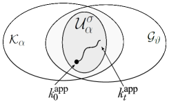
Figure 1. The evolution in spaces

Fig. 1 provides an illustration to the idea of how to realize step (i). The origin of the inequality in question is in (2.11) and (2.12). To relate $k_{t}$ with a positive measure one uses local approximations of $\mu_{0}$, the densities of which (not necessarily normalized) evolve $R^{\rm app}_{0}\to R^{\rm app}_{t}$ in $L^{1}$-like spaces according to Theorem 4.1. These approximations are tailored in such a way that the corresponding correlation functions (2.9) (that have the desired property by construction) also evolve $q_{0}^{\rm app}\to q_{t}^{\rm app}$ in $L^{1}$-like spaces $\mathcal{G}_{\vartheta}$. The technique developed in Sect. 5 allows for proving that $\langle\!\langle G,k_{t}^{\rm app}\rangle\!\rangle$ converges to $\langle\!\langle G,k_{t}\rangle\!\rangle$ only if $k_{t}^{\rm app}=Q_{\alpha\alpha_{0}}(t)q_{0}^{\rm app}$. That is, at this stage there is no connection between the evolutions $q_{0}^{\rm app}\to q_{t}^{\rm app}$ and $q_{0}^{\rm app}\to k_{t}^{\rm app}$ as they take place in (different) spaces, $\mathcal{G}_{\vartheta}$ and $\mathcal{K}_{\alpha}$, respectively. It turns out, that these spaces have an intersection $\mathcal{U}_{\alpha}^{\sigma}$ constructed with the help of some objects dependent on a para,eter, $\sigma>0$. To employ this fact we use auxiliary models (indexed by $\sigma$), for which we prove that both evolutions $q_{0}^{\rm app}\to q_{t}^{\rm app}$ and $q_{0}^{\rm app}=k_{0}^{\rm app}\to k_{t}^{\rm app}$ take place in $\mathcal{U}_{\alpha}^{\sigma}$ and thus coincide. That is $q_{t}^{\rm app}=k_{t}^{\rm app}$ for $t\leq\tau$ with some positive $\tau$, that yields the desired positivity of $k_{t}^{\rm app}$. Then step (ii) includes also taking the limit $\sigma\to 0^{+}$.

6.1. Auxiliary evolutions

For $\sigma>0$ and $x\in\mathds{R}^{d}$, we set

$$\phi_{\sigma}(x)=\exp\left(-\sigma|x|^{2}\right),\quad\langle\phi_{\sigma}\rangle=\int_{\mathds{R}^{d}}\phi_{\sigma}(x)dx.$$ (6.1)

$$b_{\sigma}(x|y_{1},y_{2})=b(x|y_{1},y_{2})\phi_{\sigma}(y_{1})\phi_{\sigma}(y_{2}).$$

Consider

$$L^{\Delta,\sigma}=A^{\Delta,\sigma}+B^{\Delta,\sigma}=A_{\upsilon}^{\Delta,\sigma}+B_{\upsilon}^{\Delta,\sigma},$$ (6.2)

that is obtained from the corresponding operators in (4.2) and (5.11), (5.12) by replacing $b$ with $b_{\sigma}$ given in (6.1). Since this substitution does not affect $\mathcal{D}^{\Delta}_{\alpha}$, see (4.5), we will use the latter as the domain of the corresponding unbounded operators. Then we repeat the construction as in the proof of Lemma 5.4 and obtain the family $\{Q^{\sigma}_{\alpha_{2}\alpha_{1}}(t):(\alpha_{1},\alpha_{2},t)\in\mathcal{A}(B^{\Delta}_{\upsilon})\}$ corresponding to the choice $\mathbf{B}=B_{\upsilon}^{\Delta,\sigma}$. Along with the evolution $t\mapsto Q^{\sigma}_{\alpha_{2}\alpha_{1}}(t)k_{0}$ we will consider two more evolutions in $L^{\infty}$- and $L^{1}$-like spaces. The latter one will be positive in the sense of Proposition 2.3 by the very construction. The auxiliary $L^{\infty}$-like space where we are going to construct $t\mapsto k_{t}^{\rm app}$ lies in the intersection of the just mentioned $L^{1}$-like space with the spaces $\mathcal{K}_{\alpha}$, see Fig. 1, and hence is also positive in the sense of Proposition 2.3. These arguments will allow us to realize item (i) of the program.

6.1.1. $L^{\infty}$-like evolution

For $u:\Gamma_{0}\to\mathbb{R}$, we define the norm

$$\|u\|_{\sigma,\alpha}=\operatorname*{\mathrm{ess\,sup}}_{\eta\in\Gamma_{0}}\frac{|u(\eta)|\exp(-\alpha|\eta|)}{e(\phi_{\sigma};\eta)},$$ (6.3)

where

$$e(\phi_{\sigma};\eta)=\prod_{x\in\eta}\phi_{\sigma}(x)=\exp\left(-\sigma\sum_{x\in\eta}|x|^{2}\right),$$

cf. (2.7). Then we consider the Banach space $\mathcal{U}_{\sigma,\alpha}=\{u:\Gamma_{0}\to\mathbb{R}:\|u\|_{\sigma,\alpha}<\infty\}$. Clearly,

$$\mathcal{U}_{\sigma,\alpha}\hookrightarrow\mathcal{K}_{\alpha},\qquad\alpha\in\mathds{R}.$$ (6.4)

The space predual to $\mathcal{U}_{\sigma,\alpha}$ is the $L^{1}$-space equipped with the norm, cf. (5.3), (5.4),

$$|G|_{\sigma,\alpha}=\int_{\Gamma_{0}}|G(\eta)|\exp(\alpha|\eta|)e(\phi_{\sigma};\eta)\lambda(d\eta).$$ (6.5)

In this space, we define $A^{\sigma}_{1,\upsilon}$ which acts exactly as in (5.5), and $A^{\sigma}_{2}$ which acts as in (5.5) with $b$ replaced by $b_{\sigma}$. Their domain is the same $\mathcal{D}_{\alpha}$. Then, like in (5.2), by means of (2.14) and (6.5) we obtain

$$|A_{2}^{\sigma}G|_{\sigma,\alpha} = \int_{\Gamma_{0}}\left(\sum_{x\in\eta}\int_{(\mathds{R}^{d})^{2}}|G(\eta\setminus x\cup\{y_{1},y_{2}\})|b_{\sigma}(x|y_{1},y_{2})dy_{1}dy_{2}\right)$$

$$\times \exp(\alpha|\eta|)e(\phi_{\sigma};\eta)\lambda(d\eta)$$

$$= e^{\alpha}\int_{\Gamma_{0}}\left(\int_{(\mathds{R}^{d})^{3}}|G(\eta\cup\{y_{1},y_{2}\})|b_{\sigma}(x|y_{1},y_{2})\phi_{\sigma}(x)dxdy_{1}dy_{2}\right)$$

$$\times \exp(\alpha|\eta|)e(\phi_{\sigma};\eta)\lambda(d\eta)$$

$$\leq e^{\alpha}\int_{\Gamma_{0}}\left(\int_{(\mathds{R}^{d})^{2}}|G(\eta\cup\{y_{1},y_{2}\})|\beta(y_{2}-y_{1})e(\phi_{\sigma};\eta\cup\{y_{1},y_{2}\})dy_{1}dy_{2}\right)$$

$$\times \exp(\alpha|\eta|)\lambda(d\eta)$$

$$= e^{-\alpha}\int_{\Gamma_{0}}E^{b}(\eta)|G(\eta)|e^{\alpha|\eta|}e(\phi_{\sigma};\eta)\lambda(d\eta)$$

$$\leq (e^{-\alpha}/\omega)\int_{\Gamma_{0}}e^{\alpha|\eta|}\Psi_{\upsilon}(\eta)|G(\eta)|e(\phi;\eta)\lambda(d\eta)$$

$$= (e^{-\alpha}/\omega)|A_{1,\upsilon}^{\sigma}G|_{\sigma,\alpha}.$$

This allows us to prove the following analog of Lemma 5.2.

Proposition 6.2.

Let $\upsilon$ and $\omega$ be as in Proposition 2.5 and $A_{1,\upsilon}^{\sigma}$, $A_{2}^{\sigma}$ and $\mathcal{D}_{\alpha}$ be as just described. Then for each $\alpha>-\log\omega$, the operator $(A_{\upsilon}^{\sigma},\mathcal{D}_{\alpha}):=(A^{\sigma}_{1,\upsilon}+A^{\sigma}_{2},\mathcal{D}_{\alpha})$ is the generator of a sub-stochastic semigroup $S_{\sigma,\alpha}=\{S_{\sigma,\alpha}(t)\}_{t\geq 0}$ on $\mathcal{G}_{\sigma,\alpha}$.

Let $S_{\sigma,\alpha}^{\odot}$ be the sun-dual semigroup, the definition of which is pretty analogous to that of $S_{\alpha}^{\odot}$, see Proposition 5.3. Then, for $\alpha^{\prime}<\alpha$, we define $\Sigma_{\alpha\alpha^{\prime}}^{\sigma}(t)=S^{\odot}_{\sigma,\alpha}(t)|_{\mathcal{U}_{\sigma.\alpha^{\prime}}}$. As in Proposition 5.3 we then get that the map

$$[0,+\infty)\ni t\mapsto\Sigma_{\alpha\alpha^{\prime}}^{\sigma}(t)\in\mathcal{L}(\mathcal{U}_{\sigma,\alpha^{\prime}},\mathcal{U}_{\sigma,\alpha})$$

is continuous and

$$\|\Sigma_{\alpha,\alpha^{\prime}}^{\sigma}(t)\|\leq 1,\qquad{\rm for}\ {\rm all}\ t\geq 0.$$

The operators $B^{\Delta,\sigma}_{\upsilon}=B^{\Delta,\sigma}_{1}+B^{\Delta,\sigma}_{2,\upsilon}$ act as in (5.12) with $b$ replaced by $b_{\sigma}$. Then we define the corresponding bounded operators and obtain, cf. (5.13),

$$\|(B^{\Delta,\sigma}_{\upsilon})_{\alpha\alpha^{\prime}}\|\leq\frac{2\langle b\rangle+\upsilon+\langle a\rangle e^{\alpha^{\prime}}}{e(\alpha-\alpha^{\prime})}.$$

Thereafter, we take $\delta>0$ as in Lemma 5.4 and the division as in (5.22), and then define

$$\Pi_{\alpha\alpha^{\prime}}^{l,\sigma}(t,t_{1},t_{2},...,t_{l}) = \Sigma_{\alpha\alpha^{2l}}^{\sigma}(t-t_{1})(B_{\upsilon}^{\Delta,\sigma})_{\alpha^{2l}\alpha^{2l-1}}\cdots\Sigma_{\alpha^{2s+1}\alpha^{2s}}^{\sigma}(t_{l-s}-t_{l-s+1})$$

$$\times (B_{\upsilon}^{\Delta,\sigma})_{\alpha^{2s}\alpha^{2s-1}}\cdots\Sigma_{\alpha^{3}\alpha^{2}}^{\sigma}(t_{l-1}-t_{l})(B_{\upsilon}^{\Delta,\sigma})_{\alpha^{2}\alpha^{1}}\Sigma_{\alpha^{1}\alpha^{\prime}}^{\sigma}(t_{l}),$$

As in the proof of Lemma 5.4 we obtain the family $\{U^{\sigma}_{\alpha_{2}\alpha_{1}}(t):(\alpha_{1},\alpha_{2},t)\in\mathcal{A}(B^{\Delta}_{\upsilon})\}$, see (5.19), with members defined by

$$U^{\sigma}_{\alpha_{2}\alpha_{1}}(t)=\Sigma_{\alpha_{2}\alpha_{1}}^{\sigma}(t)+\sum_{l=1}^{\infty}\int_{0}^{t}\int_{0}^{t_{1}}...\int_{0}^{t_{l-1}}\Pi^{l,\sigma}_{\alpha_{2}\alpha_{1}}(t,t_{1},t_{2},...,t_{l})dt_{l}...dt_{1},$$

where the series converges for $t<T(\alpha_{2},\alpha_{1})$ defined in (5.2), cf. (5.18) and (5.27). For this family, the following holds, cf. (5.21),

$$\frac{d}{dt}U^{\sigma}_{\alpha_{2}\alpha_{1}}(t)=L^{\Delta,\sigma}_{\alpha_{2},u}U^{\sigma}_{\alpha_{2}\alpha_{1}}(t),$$ (6.6)

where the action of of $L^{\Delta,\sigma}_{\alpha_{2},u}$ is as in (6.2) and the domain is

$$\mathcal{D}^{\Delta,\sigma}_{\alpha_{2},u}=\{u\in\mathcal{U}_{\sigma,\alpha_{2}}:\Psi_{\upsilon}u\in\mathcal{U}_{\sigma,\alpha_{2}}\}\subset\mathcal{D}^{\Delta}_{\alpha_{2}},$$ (6.7)

where the latter inclusion follows by (6.4) and (4.5). Then by (6.7) we have that

$$L^{\Delta,\sigma}_{\alpha,u}u=L^{\Delta,\sigma}_{\alpha}u,\qquad u\in\mathcal{D}^{\Delta,\sigma}_{\alpha,u}.$$ (6.8)

Now by (6.6) we prove the following statement.

Proposition 6.3.

For each $\alpha_{2}>\alpha_{1}>-\log\omega$, the problem

$$\dot{u}_{t}=L^{\Delta,\sigma}_{\alpha_{2},u}u_{t},\qquad u_{t}|_{t=0}=u_{0}\in\mathcal{U}_{\sigma,\alpha_{1}}$$ (6.9)

has a unique solution $u_{t}\in\mathcal{U}_{\sigma,\alpha_{2}}$ on the time interval $[0,T(\alpha_{2},\alpha_{1}))$. This solution is given by $u_{t}=U^{\sigma}_{\alpha_{2}\alpha_{1}}(t)u_{0}$.

Corollary 6.4.

Let $\alpha_{2}>\alpha_{1}>-\log\omega$ be as in Proposition 6.3 and $Q^{\sigma}_{\alpha_{2}\alpha_{1}}(t)$ be as described at the beginning of this subsection. Then for each $t<T(\alpha_{2},\alpha_{1})$ and $u_{0}\in\mathcal{U}_{\sigma,\alpha_{1}}\subset\mathcal{K}_{\alpha_{1}}$, it follows that

$$U^{\sigma}_{\alpha_{2}\alpha_{1}}(t)u_{0}=Q^{\sigma}_{\alpha_{2}\alpha_{1}}(t)u_{0}.$$ (6.10)

Proof.

By (6.8) we get that the solution of (6.9) is also the unique solution of the following “$\sigma$-analog” of (5.1)

$$\dot{u}_{t}=L^{\Delta,\sigma}_{\alpha_{2}}u_{t},\quad u_{t}|_{t=0}=u_{0},$$

and hence is given by the right-hand side of (6.10). Then the equality in (6.10) follows by the uniqueness just mentioned. ∎

6.1.2. $L^{1}$-like evolution

Now we take $L^{\Delta,\sigma}$ as given in (6.2) and define the corresponding operator $L^{\Delta,\sigma}_{\vartheta}$ in $\mathcal{G}_{\vartheta}$, $\vartheta\in\mathds{R}$, introduced in (5.3), (5.4), with domain $\mathcal{D}_{\vartheta}$ given in (5.5). By (6.2) and (4.2) we have that $A^{\Delta}_{1}:\mathcal{D}_{\vartheta}\to\mathcal{G}_{\vartheta}$. Next, for $q\in\mathcal{D}_{\vartheta}$, we have

$$|A^{\Delta,\sigma}_{2}q|_{\vartheta} \leq \int_{\Gamma_{0}}e^{\vartheta|\eta|}\left(\int_{\mathds{R}^{d}}\sum_{y_{1}\in\eta}\sum_{y_{2}\in\eta\setminus y_{1}}|q(\eta\cup x\setminus\{y_{1},y_{2}\})|b_{\sigma}(x|y_{1}.y_{2})dx\right)\lambda(d\eta)\qquad\quad$$

$$\leq \int_{\Gamma_{0}}e^{\vartheta|\eta|+2\vartheta}\int_{\mathds{R}^{d}}|q(\eta\cup x)|\left(\int_{(\mathds{R}^{d})^{2}}b(x|y_{1},y_{2})dy_{1}dy_{2}\right)dx\lambda(d\eta)$$

$$= \langle b\rangle e^{\vartheta}\int_{\Gamma_{0}}|\eta|e^{\vartheta|\eta|}|q(\eta)|\lambda(d\eta)\leq e^{\vartheta}\int_{\Gamma_{0}}\Psi(\eta)e^{\vartheta|\eta|}|q(\eta)|\lambda(d\eta),$$

see item (iii) of Assumption 1 and (3.3). Hence, $A^{\Delta,\sigma}_{2}:\mathcal{D}_{\vartheta}\to\mathcal{G}_{\vartheta}$. Next, for the same $q$, we have

$$|B^{\Delta}_{1}q|_{\vartheta} \leq \int_{\Gamma_{0}}e^{\vartheta|\eta|}\left(\int_{\mathds{R}^{d}}|q(\eta\cup x)|E^{a}(x,\eta)dx\right)\lambda(d\eta)$$

$$= e^{-\vartheta}\int_{\Gamma_{0}}e^{\vartheta|\eta|}E^{a}(\eta)|q(\eta)|\lambda(d\eta)\leq e^{-\vartheta}\int_{\Gamma_{0}}\Psi(\eta)e^{\vartheta|\eta|}|q(\eta)|\lambda(d\eta).$$

Hence, $B^{\Delta}_{1}:\mathcal{D}_{\vartheta}\to\mathcal{G}_{\vartheta}$. Finally,

$$|B^{\Delta,\sigma}_{2}q|_{\vartheta} \leq 2\int_{\Gamma_{0}}e^{\vartheta|\eta|}\left(\int_{(\mathds{R}^{d})^{2}}\sum_{y_{1}\in\eta}|q(\eta\cup x\setminus y_{1})|b_{\sigma}(x|y_{1},y_{2})dy_{2}dx\right)\lambda(d\eta)\qquad$$

$$\leq 2\int_{\Gamma_{0}}e^{\vartheta|\eta|+\vartheta}\left(\int_{(\mathds{R}^{d})^{3}}|q(\eta\cup x)|b(x|y_{1},y_{2})dxdy_{1}dy_{2}\right)\lambda(d\eta)\qquad$$

$$= 2\langle b\rangle\int_{\Gamma_{0}}e^{\vartheta|\eta|}|\eta||q(\eta)|\lambda(d\eta)\leq\int_{\Gamma_{0}}\Psi(\eta)e^{\vartheta|\eta|}|q(\eta)|\lambda(d\eta).$$

Then by (6.1.2), (6.1.2) and (6.1.2) we conclude that, for an arbitrary $\vartheta\in\mathds{R}$, $L^{\Delta,\sigma}=A^{\Delta}_{1}+A^{\Delta,\sigma}_{2}+B^{\Delta}_{1}+B^{\Delta,\sigma}_{2}$ maps $\mathcal{D}_{\vartheta}$ to $\mathcal{G}_{\vartheta}$ and hence can be used to define the corresponding unbounded operator $(L^{\Delta,\sigma}_{\vartheta},\mathcal{D}_{\vartheta})$. Let us then consider the corresponding Cauchy problem

$$\dot{q}_{t}=L^{\Delta,\sigma}_{\vartheta}q_{t},\qquad q_{t}|_{t=0}=q_{0}\in\mathcal{D}_{\vartheta}.$$ (6.14)

Recall that $\mathcal{G}_{\vartheta^{\prime}}\subset\mathcal{D}_{\vartheta}$ for each $\vartheta^{\prime}>\vartheta$.

Lemma 6.5.

For a given $\vartheta>0$ and $\vartheta^{\prime}>\vartheta$, assume that the problem in (6.14) with $q_{0}\in\mathcal{G}_{\vartheta^{\prime}}$ has a solution $q_{t}\in\mathcal{G}_{\vartheta}$ on a time interval $[0,\tau)$. Then this solution is unique.

Proof.

Set

$$w_{t}(\eta)=(-1)^{|\eta|}q_{t}(\eta).$$

Then $|w_{t}|_{\vartheta}=|q_{t}|_{\vartheta}$ and $q_{t}$ solves (6.14) if and only if $w_{t}$ solves the following equation

$$\dot{w}_{t}=\left(A_{1}^{\Delta}-A_{2}^{\Delta,\sigma}-B_{1}^{\Delta}+B_{2}^{\Delta,\sigma}\right)w_{t}.$$ (6.15)

By Proposition 3.2 we prove that $(A_{1}^{\Delta}-B_{1}^{\Delta},\mathcal{D}_{\vartheta})$ generates a sub-stochastic semigroup on $\mathcal{G}_{\vartheta}$. Indeed, $(A_{1}^{\Delta},\mathcal{D}_{\vartheta})$ generates a sub-stochastic semigroup defined in (5.7) with $\upsilon=0$, and $-B_{1}^{\Delta}$ is positive and defined on $\mathcal{D}_{\vartheta}$, see (6.1.2). Also by (6.1.2), for $w\in\mathcal{G}^{+}_{\vartheta}$ and $r\in(0,1)$, we get

$$\int_{\Gamma_{0}}e^{\vartheta|\eta|}\left(\left(A_{1}^{\Delta}-r^{-1}B_{1}^{\Delta}\right)w\right)(\eta)\lambda(d\eta)=-\int_{\Gamma_{0}}e^{\vartheta|\eta|}\Psi(\eta)w(\eta)\lambda(d\eta)$$

$$+r^{-1}\int_{\Gamma_{0}}e^{\vartheta|\eta|}\left(\int_{\mathds{R}^{d}}w(\eta\cup x)E^{a}(x,\eta)dx\right)\lambda(d\eta)$$

$$=-\int_{\Gamma_{0}}e^{\vartheta|\eta|}\Psi(\eta)w(\eta)\lambda(d\eta)+r^{-1}e^{-\vartheta}\int_{\Gamma_{0}}e^{\vartheta|\eta|}E^{a}(\eta)w(\eta)\lambda(d\eta)$$

$$\leq-\left(1-r^{-1}e^{-\vartheta}\right)\int_{\Gamma_{0}}\Psi(\eta)e^{\vartheta|\eta|}w(\eta)\lambda(d\eta)\leq 0,$$

where the latter inequality holds for $r\in(e^{-\vartheta},1)$. Therefore, $(A_{1}^{\Delta}-B_{1}^{\Delta},\mathcal{D}_{\vartheta})=(A_{1}^{\Delta}-rr^{-1}B_{1}^{\Delta},\mathcal{D}_{\vartheta})$ generates a sub-stochastic semigroup $V_{\vartheta}=\{V_{\vartheta}(t)\}_{t\geq 0}$ on $\mathcal{G}_{\vartheta}$. For each $\vartheta^{\prime\prime}\in(0,\vartheta)$, we have that $\mathcal{G}_{\vartheta}\hookrightarrow\mathcal{G}_{\vartheta^{\prime\prime}}$. By the estimates in (6.1.2) and (6.1.2), similarly as in (5.13) we obtain that

$$|A^{\Delta,\sigma}_{2}w|_{\vartheta^{\prime\prime}} \leq \frac{\langle b\rangle}{e(\vartheta-\vartheta^{\prime\prime})}|w|_{\vartheta},$$

$$|B^{\Delta,\sigma}_{2}w|_{\vartheta^{\prime\prime}} \leq \frac{2\langle b\rangle}{e(\vartheta-\vartheta^{\prime\prime})}|w|_{\vartheta},$$

which we then use to define a bounded operator $C^{\Delta,\sigma}_{\vartheta^{\prime\prime}\vartheta}:\mathcal{G}_{\vartheta}\to\mathcal{G}_{\vartheta^{\prime\prime}}$. It acts as $-A^{\Delta,\sigma}_{2}+B^{\Delta,\sigma}_{2}$ and its norm satisfies

$$\|C^{\Delta,\sigma}_{\vartheta^{\prime\prime}\vartheta}\|\leq\frac{3\langle b\rangle}{e(\vartheta-\vartheta^{\prime\prime})}.$$ (6.16)

Assume now that (6.15) has two solutions corresponding to the same initial condition $w_{0}$. Let $v_{t}$ be their difference. Then it solves (6.15) with the zero initial condition and hence satisfies

$$v_{t}=\int_{0}^{t}V_{\vartheta^{\prime\prime}}(t-s)C^{\Delta,\sigma}_{\vartheta^{\prime\prime}\vartheta}v_{s}ds$$ (6.17)

where $v_{t}$ in the left-hand side is considered as an element of $\mathcal{G}_{\vartheta^{\prime\prime}}$ and $t>0$ will be chosen later. Now for a given $n\in\mathds{N}$, we set $\epsilon=(\vartheta-\vartheta^{\prime\prime})/n$ and $\vartheta^{l}=\vartheta-l\epsilon$, $l=0,\dots,n$. Next, we iterate (6.17) due times and get

$$v_{t} = \int_{0}^{t}\int_{0}^{t_{1}}\cdots\int_{0}^{t_{n-1}}V_{\vartheta^{\prime\prime}}(t-t_{1})C^{\Delta,\sigma}_{\vartheta^{\prime\prime}\vartheta^{n-1}}V_{\vartheta^{n-1}}(t_{1}-t_{2})C^{\Delta,\sigma}_{\vartheta^{n-1}\vartheta^{n-2}}\times\cdots\times$$

$$\times V_{\vartheta^{1}}(t_{n-1}-t_{n})C^{\Delta,\sigma}_{\vartheta^{n-1}\vartheta}v_{t_{n}}dt_{n}\cdots dt_{1}.$$

Then we take into account that $V_{\vartheta}$ is sub-stochastic, $C^{\Delta,\sigma}_{\vartheta^{l}\vartheta^{l-1}}$ are positive and satisfy (6.16), and thus obtain from the latter that $v_{t}$ satisfies

$$|v_{t}|_{\vartheta^{\prime\prime}}\leq\frac{1}{n!}\left(\frac{n}{e}\right)^{n}\left(\frac{3t\langle b\rangle}{\vartheta-\vartheta^{\prime\prime}}\right)^{n}\sup_{s\in[0,t]}|v_{s}|_{\vartheta}.$$

Then, since $n$ is an arbitrary positive integer, for all $t<(\vartheta-\vartheta^{\prime\prime})/3\langle b\rangle$ it follows that $v_{t}=0$. To prove that $v_{t}=0$ for all $t$ of interest one has to repeat the above procedure appropriate number of times. ∎

Let us now take $u\in\mathcal{U}_{\sigma,\alpha}$ with some $\alpha\in\mathds{R}$, for which by (6.3) we have

$$|u(\eta)|\leq\|u\|_{\sigma,\alpha}e^{\alpha|\eta|}e(\phi_{\sigma},\eta).$$

Then the norm of this $u$ in $\mathcal{G}_{\vartheta}$ can be estimated as follows, see (6.1),

$$|u|_{\vartheta}\leq\|u\|_{\sigma,\alpha}\int_{\Gamma_{0}}\exp\left((\alpha+\vartheta)|\eta|\right)e(\phi_{\sigma},\eta)\lambda(d\eta)=\|u\|_{\sigma,\alpha}\exp\left((\alpha+\vartheta)\langle\phi\rangle\right).$$ (6.18)

This means that $\mathcal{U}_{\sigma,\alpha}\hookrightarrow\mathcal{G}_{\vartheta}$ for each pair of real $\alpha$ and $\vartheta$. Moreover, for the operators discussed above this implies, cf. (6.8),

$$L^{\Delta,\sigma}_{\alpha,u}u=L_{\vartheta}^{\Delta,\sigma}u,\qquad u\in\mathcal{D}^{\Delta,\sigma}_{\alpha,u}.$$ (6.19)

Corollary 6.6.

Let $\alpha_{1}$ and $\alpha_{2}$ be as in Proposition 6.3. Then, for each $q_{0}\in\mathcal{U}_{\sigma,\alpha_{1}}$, the problem in (6.14) has a unique solution $q_{t}\in\mathcal{U}_{\sigma,\alpha_{2}}$, $t<T(\alpha_{2},\alpha_{1})$, which coincides with the unique solution of (6.9).

Proof.

By (6.19) we have that the unique solution of (6.9) $u_{t}$ solves also (6.14), and this is a unique solution in view of Lemma 6.5. ∎

6.2. Local approximations

Our aim now is to prove that, cf. Proposition 2.3, the following holds

$$\langle\!\langle G,Q^{\sigma}_{\alpha_{2}\alpha_{1}}(t)k_{0}\rangle\!\rangle\geq 0,\qquad G\in B_{\rm bs}^{\star}(\Gamma_{0}),$$ (6.20)

for suitable $t>0$. By Corollaries 6.4 and 6.6 to this end it is enough to prove (6.20) with $Q^{\sigma}_{\alpha_{2}\alpha_{1}}(t)k_{0}$ replaced by $q_{t}$.

For $\mu_{0}\in\mathcal{P}_{\rm exp}(\Gamma)$ and a compact $\Lambda$, let $\mu^{\Lambda}_{0}\in\mathcal{P}(\Gamma_{\Lambda})$ be the corresponding projection to $\Gamma_{\Lambda}$ defined in (1.2). Let $R^{\Lambda}_{0}$ be its Radon-Nikodym derivative, see (2.8). For $N\in\mathds{N}$ and $\eta\in\Gamma_{0}$, we then set

$$R^{\Lambda,N}_{0}(\eta)=\left\{\begin{array}[]{ll}R^{\Lambda}_{0}(\eta),&{\rm if}\ \ \eta\in\Gamma_{\Lambda}\ \ {\rm and}\ \ |\eta|\leq N;\\[5.69046pt] 0,&{\rm otherwise}.\end{array}\right.$$ (6.21)

Until the end of this subsection, $\Lambda$ and $N$ are fixed. Having in mind (2.9) we introduce

$$q_{0}^{\Lambda,N}(\eta)=\int_{\Gamma_{0}}R^{\Lambda,N}_{0}(\eta\cup\xi)\lambda(d\xi),\qquad\eta\in\Gamma_{0}.$$ (6.22)

For $G\in B^{\star}_{\rm bs}(\Gamma_{0})$, by (2.11), (2.14) and (6.22) we have

$$\langle\!\langle G,q_{0}^{\Lambda,N}\rangle\!\rangle=\langle\!\langle KG,R_{0}^{\Lambda,N}\rangle\!\rangle\geq 0.$$ (6.23)

By (6.21) it follows that $R^{\Lambda,N}_{0}\in\mathcal{R}^{+}$ and $\|R^{\Lambda,N}_{0}\|_{\mathcal{R}}\leq 1$. Moreover, for each $\kappa>0$, we have, see (2.4),

$$\|R^{\Lambda,N}_{0}\|_{\mathcal{R}_{\chi^{\kappa}}}=\int_{\Gamma_{\Lambda}}e^{\kappa|\eta|}R^{\Lambda,N}_{0}(\eta)\lambda(d\eta)\leq e^{\kappa N}\|R^{\Lambda,N}_{0}\|_{\mathcal{R}}\leq e^{\kappa N}.$$ (6.24)

Let $S^{\sigma}_{\mathcal{R}}$ be the stochastic semigroup on $\mathcal{R}$ constructed in the proof of Theorem 3.1 with $b$ replaced by $b_{\sigma}$. Recall that $R_{t}=S_{\mathcal{R}}(t)R_{0}$ is the solution of (3.17). Set

$$R^{\Lambda,N}_{t} = S_{\mathcal{R}}^{\sigma}(t)R^{\Lambda,N}_{0},\qquad t>0,$$ (6.25)

$$q^{\Lambda,N}_{t}(\eta) = \int_{\Gamma_{0}}R^{\Lambda,N}_{t}(\eta\cup\xi)\lambda(d\xi),\quad\eta\in\Gamma_{0}.$$

Proposition 6.7.

For each $\vartheta\in\mathds{R}$ and $t\in[0,\tau_{\vartheta})$, $\tau_{\vartheta}:=[e\langle b\rangle(1+e^{\vartheta})]^{-1}$, it follows that $q^{\Lambda,N}_{t}\in\mathcal{G}_{\vartheta}^{+}$. Moreover,

$$\langle\!\langle G,q_{t}^{\Lambda,N}\rangle\!\rangle\geq 0$$ (6.26)

holding for each $G\in B^{\star}_{\rm bs}(\Gamma_{0})$ and all $t>0$.

Proof.

Since $S_{\mathcal{R}}^{\sigma}$ is stochastic and $R_{0}^{\Lambda,N}$ is as in (6.21), then $R_{t}^{\Lambda,N}\in\mathcal{R}^{+}$ for all $t>0$. Hence, $q^{\Lambda,N}_{t}(\eta)\geq 0$ for all those $t>0$ for which the integral in the second line in (6.25) makes sense. By (3.7) we have that $T(\kappa,\kappa^{\prime})$, as a function of $\kappa$, attains its maximum value $T_{\kappa^{\prime}}=e^{-\kappa^{\prime}}/e\langle b\rangle$ at $\kappa=\kappa^{\prime}+1$. By (6.24) we have that $R^{\Lambda,N}_{0}\in\mathcal{R}_{\chi^{\kappa}}$ for any $\kappa>0$. Then, for each $\kappa>0$, by Proposition 3.3 it follows that $R^{\Lambda,N}_{t}\in\mathcal{R}_{\chi^{\kappa}}$ for $t<T_{\kappa}$. Taking all these fact into account we then get

$$|q_{t}^{\Lambda,N}|_{\vartheta} = \int_{\Gamma_{0}}e^{\vartheta|\eta|}q_{t}^{\Lambda,N}(\eta)\lambda(d\eta)$$

$$= \int_{\Gamma_{0}}\int_{\Gamma_{0}}e^{\vartheta|\eta|}R^{\Lambda,N}_{t}(\eta\cup\xi)\lambda(d\eta)\lambda(d\xi)$$

$$= \int_{\Gamma_{0}}\left(1+e^{\vartheta}\right)^{|\eta|}R^{\Lambda,N}_{t}(\eta)\lambda(d\eta)=\|R^{\Lambda,N}_{t}\|_{\mathcal{R}_{\chi^{\kappa}}}$$

with $\kappa=\log(1+e^{\vartheta})$. For these $\kappa$ and $\vartheta$, we have that $T_{\kappa}=\tau_{\vartheta}$. Then $q_{t}^{\Lambda,N}\in\mathcal{G}_{\vartheta}$ for $t<\tau_{\vartheta}$, holding by (6.2). The existence of the integral in (6.26) follows by the equality

$$\langle\!\langle G,q^{\Lambda,N}_{t}\rangle\!\rangle=\langle\!\langle KG,R^{\Lambda,N}_{t}\rangle\!\rangle,$$

(2.6) and the fact that $R^{\Lambda,N}_{t}\in\mathcal{R}^{+}_{\chi_{m}}$ for all $t>0$ and $m\in\mathds{N}$, see claims (a) and (c) of Theorem 3.1. The validity of the inequality in (6.26) is straightforward, cf. (6.23). ∎

Corollary 6.8.

For each $\alpha\in\mathds{R}$, it follows that $q_{0}^{\Lambda,N}\in\mathcal{U}_{\sigma,\alpha}^{+}$.

Proof.

Set $I_{N}(\eta)=1$ whenever $|\eta|\leq N$ and $I_{N}(\eta)=0$ otherwise. By (6.21), (6.22) and (2.9) we have that

$$q_{0}^{\Lambda,N}(\eta) = I_{N}(\eta)\mathds{1}_{\Gamma_{\Lambda}}(\eta)\int_{\Gamma_{\Lambda}}R_{0}^{\Lambda}(\eta\cup\xi)\lambda(d\xi)$$

$$= k_{0}(\eta)I_{N}(\eta)\mathds{1}_{\Gamma_{\Lambda}}(\eta)\leq\varkappa^{N}I_{N}(\eta)\mathds{1}_{\Gamma_{\Lambda}}(\eta).$$

The latter estimate follows by the fact that $k_{0}=k_{\mu_{0}}$ for some $\mu_{0}\in\mathcal{P}_{\rm exp}(\Gamma)$, and thus $k_{0}(\eta)\leq\varkappa^{|\eta|}$ for some $\varkappa>0$, see Definition 2.1 and (2.2). Then $q_{0}^{\Lambda,N}\in\mathcal{U}_{\sigma,\alpha}$ by (6.3). The stated positivity i immediate. ∎

By (6.18) and Corollary 6.8 we obtain that $q_{0}^{\Lambda,N}\in\mathcal{G}_{\vartheta}^{+}$ for each $\vartheta\in\mathds{R}$. Now we relate $q_{t}^{\Lambda,N}$ with solutions of (6.14).

Lemma 6.9.

For each $\vartheta\in\mathds{R}$, the map $[0,\tau_{\vartheta})\ni t\mapsto q_{t}^{\Lambda,N}\in\mathcal{G}_{\vartheta}$ is continuous and continuously differentiable on $(0,\tau_{\vartheta})$. Moreover, $q_{t}^{\Lambda,N}\in\mathcal{D}_{\vartheta}$, see (5.5), and solves the problem in (6.14) on the time interval $[0,\tau_{\vartheta})$ with $q_{0}^{\Lambda,N}$ as the initial condition.

Proof.

Fix an arbitrary $\vartheta\in\mathds{R}$. The stated continuity of $t\mapsto q_{t}^{\Lambda,N}$ follows by (6.25). Let us prove that $q_{t}^{\Lambda,N}$ be differentiable in $\mathcal{G}_{\vartheta}$ on $(0,\tau_{\vartheta})$ and the following holds

$$\dot{q}^{\Lambda,N}_{t}(\eta)=\int_{\Gamma_{0}}\dot{R}^{\Lambda,N}_{t}(\eta\cup\xi)\lambda(d\xi).$$ (6.28)

For small enough $|\tau|$, we have

$$\frac{1}{\tau}\left(q^{\Lambda,N}_{t+\tau}(\eta)-q^{\Lambda,N}_{t}(\eta)\right)-\int_{\Gamma_{0}}\dot{R}^{\Lambda,N}_{t}(\eta\cup\xi)\lambda(d\xi)$$ (6.29)

$$\qquad=\int_{\Gamma_{0}}\left[\frac{1}{\tau}\left(R^{\Lambda,N}_{t+\tau}(\eta\cup\xi)-R^{\Lambda,N}_{t}(\eta\cup\xi)\right)-\dot{R}^{\Lambda,N}_{t}(\eta\cup\xi)\right]\lambda(d\xi).$$

Then by (2.14) we get

$$\left|{\rm LHS}(\ref{Mar2})\right|_{\vartheta}\leq\int_{\Gamma_{0}}\left(1+e^{\vartheta}\right)^{|\eta|}\left|\frac{1}{\tau}\left(R^{\Lambda,N}_{t+\tau}(\eta)-R^{\Lambda,N}_{t}(\eta)\right)-\dot{R}^{\Lambda,N}_{t}(\eta)\right|\lambda(d\eta),$$

that proves (6.28), cf. (6.2). The continuity of $t\mapsto\dot{q}^{\Lambda,N}_{t}$ follows by (6.28) and the fact that $R^{\Lambda,N}_{t}=S^{\sigma}_{\mathcal{R}}(t)R^{\Lambda,N}_{0}$, which also yields that

$$\dot{q}_{t}^{\Lambda,N}(\eta)=\int_{\Gamma_{0}}\left(L^{\dagger,\sigma}_{\vartheta}R_{t}^{\Lambda,N}\right)(\eta\cup\xi)\lambda(d\xi),$$ (6.30)

where $L^{\dagger,\sigma}_{\vartheta}$ is the trace of $L^{\dagger,\sigma}$ (the generator of $S^{\sigma}_{\mathcal{R}}$) in $\mathcal{R}_{\chi^{\kappa}}$ with $\kappa=\log(1+e^{\vartheta})$. By (5.5) it follows that $\Psi_{\upsilon}(\eta)\leq C_{\varepsilon}e^{\varepsilon|\eta|}$ holding for an arbitrary $\varepsilon>0$ and the corresponding $C_{\varepsilon}>0$. For each $t<T_{\kappa}=\tau_{\vartheta}$, one can pick $\kappa^{\prime}>\kappa$ such that $R_{t}^{\Lambda,N}\in\mathcal{R}_{\chi^{\kappa^{\prime}}}$. For these $t$ and $\kappa^{\prime}$, we thus pick $\varepsilon>0$ such that $1+e^{\vartheta+\varepsilon}=e^{\kappa^{\prime}}$, and then obtain, cf. (6.2),

$$|\Psi_{\upsilon}q_{t}^{\Lambda,N}|_{\vartheta}\leq C_{\varepsilon}\|R^{\Lambda,N}_{t}\|_{\mathcal{R}^{\chi^{\kappa^{\prime}}}}.$$ (6.31)

Hence, $q_{t}^{\Lambda,N}\in\mathcal{D}_{\vartheta}$ for this $t$. Let us now prove that $q_{t}^{\Lambda,N}$ solves (6.14). In view of (6.30), (3.10) and (6.31), to this end it is enough to prove that

$$\left(L^{\Delta}q_{t}^{\Lambda,N}\right)(\eta) = -\int_{\Gamma_{0}}\Psi(\eta\cup\xi)R^{\Lambda,N}_{t}(\eta\cup\xi)\lambda(d\xi)$$

$$+ \int_{\mathds{R}^{d}}\int_{\Gamma_{0}}\left(m(x)+E^{a}(x,\eta\cup\xi)\right)R^{\Lambda,N}_{t}(\eta\cup\xi\cup x)\lambda(d\xi)dx$$

$$+ \int_{\mathds{R}^{d}}\int_{\Gamma_{0}}\sum_{y_{1}\in\eta\cup\xi}\sum_{y_{2}\in\eta\cup\xi\setminus y_{1}}b(x|y_{1},y_{2})R^{\Lambda,N}_{t}(\eta\cup\xi\cup x\setminus\{y_{1},y_{2}\})\lambda(d\xi)dx,$$

holding point-wise in $\eta\in\Gamma_{0}$. By (3.3) and (2.15) we get

$$\Psi(\eta\cup\xi)=\Psi(\eta)+\Psi(\xi)+2\sum_{x\in\eta}\sum_{y\in\xi}a(x-y).$$ (6.33)

Let $I_{1}(\eta)$ denote the first summand in the right-hand side of (6.2). By (2.14) and (6.33) we then write it as follows

$$I_{1}(\eta) = -\Psi(\eta)q_{t}^{\Lambda,N}(\eta)-2\int_{\mathds{R}^{d}}E^{a}(x,\eta)q_{t}^{\Lambda,N}(\eta\cup x)dx$$

$$- \int_{\Gamma_{0}}\Psi(\xi)R^{\Lambda,N}_{t}(\eta\cup\xi)\lambda(d\xi).$$

To calculate the latter summand in (6.2) we again use (3.3) and (2.14) to obtain the following:

$$\int_{\Gamma_{0}}\left(\sum_{x\in\xi}m(x)\right)R^{\Lambda,N}_{t}(\eta\cup\xi)\lambda(d\xi) = \int_{\Gamma_{0}}\int_{\mathds{R}^{d}}m(x)R^{\Lambda,N}_{t}(\eta\cup\xi\cup x)\lambda(d\xi)dx\qquad\quad$$

$$= \int_{\mathds{R}^{d}}m(x)q_{t}^{\Lambda,N}(\eta\cup x)dx.$$

$$\int_{\Gamma_{0}}\left(\sum_{x\in\xi}\sum_{y\in\xi\setminus x}a(x-y)\right)R^{\Lambda,N}_{t}(\eta\cup\xi)\lambda(d\xi)$$ (6.36)

$$\quad=\int_{\Gamma_{0}}\int_{(\mathds{R}^{d})^{2}}a(x-y)R^{\Lambda,N}_{t}(\eta\cup\xi\cup\{x,y\})\lambda(d\xi)dxdy$$

$$\quad=\int_{(\mathds{R}^{d})^{2}}a(x-y)q_{t}^{\Lambda,N}(\eta\cup\{x,y\})dxdy.$$

$$\int_{\Gamma_{0}}\left(\langle b\rangle\sum_{x\in\xi}1\right)R^{\Lambda,N}_{t}(\eta\cup\xi)\lambda(d\xi)=\langle b\rangle\int_{\mathds{R}^{d}}q^{\Lambda,N}_{t}(\eta\cup x)dx.$$ (6.37)

In a similar way, we get the second $I_{2}$ (resp. the third $I_{3}$) summands of the right-hand side of (6.2) as follows

$$I_{2}(\eta) = \int_{\mathds{R}^{d}}\left(m(x)+E^{a}(x,\eta)\right)q^{\Lambda,N}_{t}(\eta\cup x)dx$$

$$+ \int_{(\mathds{R}^{d})^{2}}a(x-y)q^{\Lambda,N}_{t}(\eta\cup\{x,y\})dxdy.$$

$$I_{3}(\eta) = \int_{\mathds{R}^{d}}\sum_{y_{1}\in\eta}\sum_{y_{2}\in\eta\setminus y_{1}}b(x|y_{1},y_{2})q^{\Lambda,N}_{t}(\eta\cup x\setminus\{y_{1},y_{2}\})dx$$

$$+ 2\int_{(\mathds{R}^{d})^{2}}\sum_{y_{1}\in\eta}b(x|y_{1},y_{2})q^{\Lambda,N}_{t}(\eta\cup x\setminus y_{1})dxdy_{2}$$

$$+ \langle b\rangle\int_{\mathds{R}^{d}}q^{\Lambda,N}_{t}(\eta\cup x)dx.$$

Now we plug (6.2), (6.36) and (6.37) into (6.2), and then use it together with (6.2) and (6.2) in the right-hand side of (6.2) to get its equality with the left-hand side, see (4.2). This completes the proof. ∎

Corollary 6.10.

Let $\alpha_{1}>-\log\omega$ and $\alpha_{2}>\alpha_{1}$ be chosen. Then $k^{\Lambda,N}_{t}=Q^{\sigma}_{\alpha_{2}\alpha_{1}}(t)q_{0}^{\Lambda,N}$ has the property

$$\langle\!\langle G,k_{t}^{\Lambda,N}\rangle\!\rangle\geq 0,$$ (6.40)

holding for all $G\in B_{\rm bs}^{\star}(\Gamma_{0})$ and $t<T(\alpha_{2},\alpha_{1})$.

Proof.

The proof of (6.40) will be done by showing that $k^{\Lambda,N}_{t}=q^{\Lambda,N}_{t}$, for $t<T(\alpha_{2},\alpha_{1})$ and then by employing (6.26), which holds for all $t>0$.

By Corollary 6.8 it follows that $q_{0}^{\Lambda,N}\in\mathcal{U}_{\sigma,\alpha_{1}}$, and hence $u_{t}=U^{\sigma}_{\alpha_{2}\alpha_{1}}(t)q_{0}^{\Lambda,N}$ is a unique solution of (6.9), see Proposition 6.3. By Lemma 6.9 $q_{t}^{\Lambda,N}$ solves (6.14) on $[0,\tau_{\vartheta})$, which by Corollary 6.6 yields $u_{t}=q_{t}^{\Lambda,N}$ for $t<\min\{\tau_{\vartheta};T(\alpha_{2},\alpha_{1})\}$. If $\tau_{\vartheta}<T(\alpha_{2},\alpha_{1})$, we can continue $q_{t}^{\Lambda,N}$ beyond $\tau_{\vartheta}$ by means of the following arguments. Since $u_{t}=q_{t}^{\Lambda,N}$ lies in $\mathcal{U}_{\sigma,\alpha_{2}}$ for all $t<\min\{\tau_{\vartheta};T(\alpha_{2},\alpha_{1})\}$, by (6.18) we get that $q_{t}^{\Lambda,N}$ lies in the initial space $\mathcal{G}_{\vartheta^{\prime}}$ and hence can further by continued. Thus, $u_{t}=q_{t}^{\Lambda,N}$ for all $t<T(\alpha_{2},\alpha_{1})$. Now by (6.10) we get $q_{t}^{\Lambda,N}=u_{t}=k^{\Lambda,N}_{t}$, that completes the proof. ∎

6.3. Taking the limits

We prove that (6.40) holds when the approximation is removed. Recall that $k_{t}^{\Lambda,N}$ in (6.40) depends on $\sigma>0$, $\Lambda$ and $N$. We first take the limits $\Lambda\to\mathds{R}^{d}$ and $N\to+\infty$. Below, by an exhausting sequence $\{\Lambda_{n}\}_{n\in\mathds{N}}$ we mean a sequence of compact $\Lambda_{n}$ such that: (a) $\Lambda_{n}\subset\Lambda_{n+1}$ for all $n$; (b) for each $x\in\mathds{R}^{d}$, there exits $n$ such that $x\in\Lambda_{n}$.

Proposition 6.11.

Let $\alpha_{1}>-\log\omega$, $\alpha_{2}>\alpha_{1}$ and $k_{0}\in\mathcal{K}^{\star}_{\alpha_{1}}$ be fixed. For these $\alpha_{1}$, $\alpha_{2}$ and $t<T(\alpha_{2},\alpha_{1})$, let $k_{t}^{\Lambda,N}$ and $Q^{\sigma}_{\alpha_{2}\alpha_{1}}(t)$ be the same as in Corollary 6.10 and (6.20), respectively. Then, for each $G\in B_{\rm bs}(\Gamma_{0})$ and any $t<T(\alpha_{2},\alpha_{1})$, the following holds

$$\lim_{n\to+\infty}\lim_{l\to+\infty}\langle\!\langle G,k_{t}^{\Lambda_{n},N_{l}}\rangle\!\rangle=\langle\!\langle G,Q^{\sigma}_{\alpha_{2}\alpha_{1}}(t)k_{0}\rangle\!\rangle,$$

for arbitrary exhausting $\{\Lambda_{n}\}_{n\in\mathds{N}}$ and increasing $\{N_{l}\}_{l\in\mathds{N}}$ sequences of sets and positive integers, respectively.

The proof of this statement can be performed by the literal repetition of the proof of a similar statement given in Appendix of [3].

Recall that, for $\alpha_{2}>\alpha_{1}$, $T(\alpha_{2},\alpha_{1})$ was defined in (5.2). For these, $\alpha_{2}$, $\alpha_{1}$, we set

$$\alpha=\frac{1}{3}\alpha_{2}+\frac{2}{3}\alpha_{1},\quad\ \alpha^{\prime}=\frac{2}{3}\alpha_{2}+\frac{1}{4}\alpha_{1}.$$ (6.41)

Clearly,

$$\tau(\alpha_{2},\alpha_{1}):=\frac{1}{3}T(\alpha_{2},\alpha_{1})<\min\{T(\alpha_{2},\alpha^{\prime});T(\alpha,\alpha_{1})\}.$$ (6.42)

Lemma 6.12.

Let $\alpha_{1}$, $\alpha_{2}$ and $k_{0}$ be as in Proposition 6.11, and let $k_{t}$ be the solution of (5.1). Then for each $G\in B_{\rm bs}(\Gamma_{0})$ and $t\in[0,\tau(\alpha_{2},\alpha_{1})]$, the following holds

$$\lim_{\sigma\to 0^{+}}\langle\!\langle G,Q^{\sigma}_{\alpha_{2}\alpha_{1}}(t)k_{0}\rangle\!\rangle=\langle\!\langle G,k_{t}\rangle\!\rangle.$$ (6.43)

Proof.

We recall that the solution of (5.1) is $k_{t}=Q_{\alpha_{2}\alpha_{1}}(t)k_{0}$ with $Q_{\alpha_{2}\alpha_{1}}(t)$ given in (5.27) and $t\leq T(\alpha_{2},\alpha_{1})$, see Lemma 5.1. For $\alpha$ and $\alpha^{\prime}$ as in (6.41) and $t\leq\tau(\alpha_{2},\alpha_{1})$, write

$$Q_{\alpha_{2}\alpha_{1}}(t)k_{0} = Q^{\sigma}_{\alpha_{2}\alpha_{1}}(t)k_{0}+\Upsilon_{1}(t,\sigma)+\Upsilon_{2}(t,\sigma),$$ (6.44)

$$\Upsilon_{1}(t,\sigma) = \int_{0}^{t}Q_{\alpha_{2}\alpha^{\prime}}(t-s)\left[(A^{\Delta}_{2})_{\alpha^{\prime}\alpha}-(A^{\Delta.\sigma}_{2})_{\alpha^{\prime}\alpha}\right]Q^{\sigma}_{\alpha\alpha_{1}}(s)k_{0}ds,,$$

$$\Upsilon_{2}(t,\sigma) = \int_{0}^{t}Q_{\alpha_{2}\alpha^{\prime}}(t-s)\left[(B^{\Delta}_{2})_{\alpha^{\prime}\alpha}-(B^{\Delta,\sigma}_{2})_{\alpha^{\prime}\alpha}\right]Q^{\sigma}_{\alpha\alpha_{1}}(s)k_{0}ds.$$

The validity of (6.44) is verified by taking the $t$-derivatives from both sides and then by using e.g., (5.20). Note that the norms of the operators $(A^{\Delta}_{2})_{\alpha^{\prime}\alpha}$. $(B^{\Delta}_{2})_{\alpha^{\prime}\alpha}$, $(A^{\Delta,\sigma}_{2})_{\alpha^{\prime}\alpha}$, $(B^{\Delta.\sigma}_{2})_{\alpha^{\prime}\alpha}$ can be estimated as in (5.14). For $G$ as in (6.43), we then have

$$\langle\!\langle G,Q_{\alpha_{2}\alpha_{1}}(t)k_{0}\rangle\!\rangle-\langle\!\langle G,Q^{\sigma}_{\alpha_{2}\alpha_{1}}(t)k_{0}\rangle\!\rangle=\langle\!\langle G,\Upsilon_{1}(t,\sigma)\rangle\!\rangle+\langle\!\langle G,\Upsilon_{2}(t,\sigma)\rangle\!\rangle.$$ (6.45)

By (5.29) and (6.44) it follows that

$$\langle\!\langle G,\Upsilon_{1}(t,\sigma)\rangle\!\rangle = \int_{0}^{t}\langle\!\langle G,Q_{\alpha_{2}\alpha^{\prime}}(t-s)\left[(A^{\Delta}_{2})_{\alpha^{\prime}\alpha}-(A^{\Delta.\sigma}_{2})_{\alpha^{\prime}\alpha}\right]Q^{\sigma}_{\alpha\alpha_{1}}(s)k_{0}\rangle\!\rangle ds\qquad$$

$$= \int_{0}^{t}\langle\!\langle H_{\alpha^{\prime}\alpha_{2}}(t-s)G,v_{s}^{\sigma}\rangle\!\rangle ds=\int_{0}^{t}\langle\!\langle G_{t-s},v_{s}^{\sigma}\rangle\!\rangle ds,$$

where

$$v^{\sigma}_{s}=\left[(A^{\Delta}_{2})_{\alpha^{\prime}\alpha}-(A^{\Delta.\sigma}_{2})_{\alpha^{\prime}\alpha}\right]k^{\sigma}_{s}:=\left[(A^{\Delta}_{2})_{\alpha^{\prime}\alpha}-(A^{\Delta.\sigma}_{2})_{\alpha^{\prime}\alpha}\right]Q^{\sigma}_{\alpha\alpha_{1}}(s)k_{0}\in\mathcal{K}_{\alpha^{\prime}},$$

and

$$G_{t-s}=H_{\alpha^{\prime}\alpha_{2}}(t-s)G\in\mathcal{G}_{\alpha^{\prime}},$$ (6.46)

which makes sense since obviously $G\in\mathcal{G}_{\alpha_{2}}$. In view of (4.2) we then get

$$\int_{0}^{t}\langle\!\langle G_{t-s},v_{s}^{\sigma}\rangle\!\rangle ds=\int_{\Gamma_{0}}G_{t-s}(\eta)\bigg{(}\int_{\mathds{R}^{d}}\sum_{y_{1}\in\eta}\sum_{y_{2}\in\eta\setminus y_{1}}k^{\sigma}_{s}(\eta\cup x\setminus\{y_{1},y_{2}\})$$ (6.47)

$$\qquad\times\left[1-\phi_{\sigma}(y_{1})\phi_{\sigma}(y_{2})\right]b(x|y_{1},y_{2})dx\bigg{)}\lambda(d\eta)$$

$$\qquad=\int_{\Gamma_{0}}\bigg{(}\int_{(\mathds{R}^{d})^{3}}G_{t-s}(\eta\cup\{y_{1},y_{2}\})k^{\sigma}_{s}(\eta\cup x)$$

$$\qquad\times\left[1-\phi_{\sigma}(y_{1})\phi_{\sigma}(y_{2})\right]b(x|y_{1},y_{2})dxdy_{1}dy_{2}\bigg{)}\lambda(d\eta).$$

Since $k^{\sigma}_{s}=Q^{\sigma}_{\alpha\alpha_{1}}(s)k_{0}$ is in $\mathcal{K}_{\alpha}$, we have that

$$|k^{\sigma}_{s}(\eta\cup x)|\leq\|k^{\sigma}_{s}\|_{\alpha}e^{\alpha|\eta|+\alpha}\leq e^{\alpha|\eta|+\alpha}\frac{T(\alpha,\alpha_{1})\|k_{0}\|_{\alpha_{1}}}{T(\alpha,\alpha_{1})-\tau(\alpha_{2},\alpha_{1})},$$ (6.48)

where $\alpha$ is as in (6.41) and $s\leq t\leq\tau(\alpha_{2},\alpha_{1})$. Now for $s\leq t$, we set

$$g_{s}(y_{1},y_{2})=\int_{\Gamma_{0}}e^{\alpha|\eta|}|G_{s}(\eta\cup\{y_{1},y_{2}\})|\lambda(d\eta).$$ (6.49)

Let us show that $g_{s}\in L^{1}((\mathds{R}^{d})^{2})$. By (6.46) we have

$$\int_{(\mathds{R}^{d})^{2}}g_{s}(y_{1},y_{2})dy_{1}dy_{2}=e^{-2\alpha}\int_{\Gamma_{0}}|\eta|(|\eta|-1)e^{-(\alpha^{\prime}-\alpha)|\eta|}|G_{s}(\eta)|e^{\alpha^{\prime}|\eta|}\lambda(d\eta)\qquad$$

$$\quad\qquad\leq\frac{4e^{-2\alpha-2}}{(\alpha^{\prime}-\alpha)^{2}}|G_{s}|_{\alpha^{\prime}}\leq\frac{4e^{-2\alpha-2}T(\alpha_{2},\alpha^{\prime})|G|_{\alpha_{2}}}{(\alpha^{\prime}-\alpha)^{2}[T(\alpha_{2},\alpha^{\prime})-\tau(\alpha_{2},\alpha_{1})]}.$$

Turn now to (6.47). By means of item (iv) of Assumption 1 and by (6.48) and (6.49) we get

$$\int_{0}^{t}\left|\langle\!\langle G_{t-s},v_{s}^{\sigma}\rangle\!\rangle\right|ds$$

$$\qquad\leq\beta^{*}C(\alpha_{2},\alpha_{1})\|k_{0}\|_{\alpha_{1}}\int_{0}^{t}\int_{(\mathds{R}^{d})^{2}}g_{s}(y_{1},y_{2})\left[1-\phi_{\sigma}(y_{1})\phi_{\sigma}(y_{2})\right]dsdy_{1}dy_{2},$$

where we have taken into account that $\alpha$ and $\alpha^{\prime}$ are expressed through $\alpha_{2}$ and $\alpha_{1}$, see (6.41). Then the function under the latter integral is bounded from above by $g_{s}(y_{1},y_{2})$ which by (6.3) is integrable on $[0,t]\times(\mathds{R}^{d})^{2}$. Since this function converges point-wise to $0$ as $\sigma\to 0^{+}$, by Lebesgue’s dominated convergence theorem we get that

$$\langle\!\langle G,\Upsilon_{1}(t,\sigma)\rangle\!\rangle\to 0,\qquad{\rm as}\ \ \sigma\to 0^{+}.$$

The proof that the second summand in the right-hand side of (6.45) vanishes in the limit $\sigma\to 0^{+}$ is pretty analogous. ∎

Proof of Lemma 6.1. By (4.11) and Proposition 2.3 we have that each $k_{0}\in\mathcal{K}^{\star}_{\alpha_{1}}$ is the correlation function of some $\mu_{0}\in\mathcal{P}_{\rm exp}(\Gamma_{0})$. By (4.2) we readily conclude that

$$\dot{k}_{t}(\varnothing)=(L^{\Delta}_{\alpha_{2}}k_{t})(\varnothing)=0.$$

Hence, $k_{t}(\varnothing)=k_{0}(\varnothing)=1$. At the same time, for $t\leq\tau(\alpha_{2},\alpha_{1})$ given in (6.42), we have that

$$\langle\!\langle G,k_{t}\rangle\!\rangle=\lim_{\sigma\to 0^{+}}\lim_{n\to+\infty}\lim_{l\to+\infty}\langle\!\langle G,k_{t}^{\Lambda_{n},N_{l}}\rangle\!\rangle,$$

that follows by Lemma 6.12 and Proposition 6.11. Then $\langle\!\langle G,k_{t}\rangle\!\rangle\geq 0$ by (6.40) that completes the proof. $\square$

7. The Global Solution

In this section, we continue the solution obtained in Lemma 5.1 to all $t>0$ and thus prove that it satisfies the upper bound following from property (i) in Theorem 4.1.

7.1. Comparison statements

Note that the time bound $T(\alpha,\alpha_{1})$ defined in (5.2) is a bounded function of $\alpha>\alpha_{1}$. Then the solution obtained in Lemma 5.1 may abandon the scale of spaces $\{\mathcal{K}_{\alpha}\}_{\alpha\in\mathds{R}}$ in finite time. To overcome this difficulty we compare $k_{t}$ with some auxiliary functions.

Lemma 7.1.

Let $\alpha_{2}$, $\alpha_{1}$ and $\tau(\alpha_{2},\alpha_{1})$ be as in Lemma 6.1. Then for each $t\in[0,\tau(\alpha_{2},\alpha_{1})]$ and arbitrary $k_{0}\in\mathcal{K}_{\alpha_{1}}^{\star}$, the following holds

$$0\leq(Q_{\alpha_{2}\alpha_{1}}(t;B_{\upsilon}^{\Delta})k_{0})(\eta)\leq(Q_{\alpha_{2}\alpha_{1}}(t;B_{2,\upsilon}^{\Delta})k_{0})(\eta),\qquad\eta\in\Gamma_{0}.$$ (7.1)

Proof.

The left-hand side inequality follows by Lemma 6.1 and (4.12). By the second line in (5.21) we conclude that $w_{t}=Q_{\alpha_{2}\alpha_{1}}(t;B_{2,\upsilon}^{\Delta})k_{0}$ is the unique solution of the equation

$$\dot{w}_{t}=((A^{\Delta}_{\upsilon})_{\alpha_{2}}+(B^{\Delta}_{2,\upsilon})_{\alpha_{2}})w_{t},\qquad w_{t}|_{t=0}=k_{0},$$

on the time interval $[0,T(\alpha_{2},\alpha_{1};B_{2,\upsilon}^{\Delta}))\supset[0,T(\alpha_{2},\alpha_{1};B_{\upsilon}^{\Delta}))$ since $T(\alpha_{2},\alpha_{1};B_{\upsilon}^{\Delta})\leq T(\alpha_{2},\alpha_{1};B_{2,\upsilon}^{\Delta})$. Then we have that $w_{t}-k_{t}\in\mathcal{K}_{\alpha_{2}}$ for all $t\leq\tau(\alpha_{2},\alpha_{1})$. Now we choose $\alpha^{\prime},\alpha\in[\alpha_{1},\alpha_{2}]$ according to (6.41) so that (6.42) holds, and then write

$$w_{t}-k_{t} = (Q_{\alpha_{2}\alpha_{1}}(t;B_{2,\upsilon}^{\Delta})k_{0})(\eta)-(Q_{\alpha_{2}\alpha_{1}}(t;B_{\upsilon}^{\Delta})k_{0})(\eta)$$

$$= \int_{0}^{t}Q_{\alpha_{2}\alpha^{\prime}}(t-s;B_{2,\upsilon}^{\Delta})(-B_{1}^{\Delta})_{\alpha^{\prime}\alpha}k_{s}ds,\qquad t<\tau(\alpha_{2},\alpha_{1}),$$

where the operator $(-B_{1}^{\Delta})_{\alpha^{\prime}\alpha}$ is positive with respect to the cone $\mathcal{K}_{\alpha}^{+}$ defined in (4.12). In the integral in (7.1), for all $s\in[0,\tau(\alpha_{2},\alpha_{1})]$, we have that $k_{s}\in\mathcal{K}_{\alpha}$ and $Q_{\alpha_{2}\alpha^{\prime}}(t-s;B_{2,\upsilon}^{\Delta})\in\mathcal{L}(\mathcal{K}_{\alpha^{\prime}},\mathcal{K}_{\alpha_{2}})$ is positive. We also have that $k_{s}\in\mathcal{K}_{\alpha}^{\star}\subset\mathcal{K}_{\alpha}^{+}$ (by Lemma 6.1). Therefore $w_{t}-k_{t}\in\mathcal{K}_{\alpha_{2}}^{+}$ for $t\leq\tau(\alpha_{2},\alpha_{1})$, which yields (7.1). ∎

The next step is to compare $k_{t}$ with

$$r_{t}(\eta)=\|k_{0}\|_{\alpha_{1}}\exp\left((\alpha_{1}+ct)|\eta|\right),$$ (7.3)

where $\alpha_{1}$ is as in Lemma 7.1 and

$$c=\langle b\rangle+\upsilon-m_{*},\qquad m_{*}=\inf_{x\in\mathds{R}^{d}}m(x).$$ (7.4)

Let us show that $r_{t}\in\mathcal{K}_{\alpha}$ for $t\leq\tau(\alpha_{2},\alpha_{1})$, where $\alpha$ is given in (6.41). In view of (4.3), this is the case if the following holds

$$\alpha_{1}+c\tau(\alpha_{2},\alpha_{1})\leq\frac{1}{3}\alpha_{2}+\frac{2}{3}\alpha_{1},$$ (7.5)

which amounts to $c\leq 2\langle b\rangle+\upsilon+\langle a\rangle e^{\alpha_{2}}$, see (6.42) and (5.2). The latter obviously holds by (7.4).

Lemma 7.2.

Let $\alpha_{1}$, $\alpha_{2}$ and $k_{t}=Q_{\alpha_{2}\alpha_{1}}(t)k_{0}$ be as in Lemma 7.1, and $r_{t}$ be as in (7.3), (7.4). Then $k_{t}(\eta)\leq r_{t}(\eta)$ for all $t\leq\tau(\alpha_{2},\alpha_{1})$ and $\eta\in\Gamma_{0}$.

Proof.

The idea is to show that $w_{t}(\eta)\leq r_{t}(\eta)$ and then to apply the estimate obtained in Lemma 7.1. Set $\tilde{w}_{t}=Q_{\alpha_{2}\alpha_{1}}(t;B_{2,\upsilon}^{\Delta})r_{0}$. Since $k_{0}\in\mathcal{K}_{\alpha_{1}}$, we have that $k_{0}\leq r_{0}$. Then by the positivity discussed in Remark 5.6 we obtain $w_{t}\leq\tilde{w}_{t}$, and hence $k_{t}\leq\tilde{w}_{t}$, holding for all $t\leq\tau(\alpha_{2},\alpha_{1})$. Thus, it remains to prove that $\tilde{w}_{t}(\eta)\leq r_{t}(\eta)$. To this end we write, cf. (7.1),

$$\tilde{w}_{t}-r_{t}=\int_{0}^{t}Q_{\alpha_{2}\alpha^{\prime}}(t-s;B_{2,\upsilon}^{\Delta})D_{\alpha^{\prime}\alpha}r_{s}ds,$$ (7.6)

where $\alpha^{\prime}$ and $\alpha$ are as in (6.41) and the bounded operator $D_{\alpha^{\prime}\alpha}$ acts as follows: $D=A^{\Delta}_{\upsilon}+B^{\Delta}_{2,\upsilon}-J_{c}$, where $(J_{c}k)(\eta)=c|\eta|k(\eta)$ with $c$ as in (7.4). The validity of (7.6) can be established by taking the $t$-derivative of both sides and then taking into account (7.3) and (5.21). Note that $r_{s}$ in (7.6) lies in $\mathcal{K}_{\alpha}$, as it was shown above. By means of (4.2) the action of $D$ on $r_{s}$ can be calculated explicitly yielding

$$(Dr_{t})(\eta) = -\Psi_{\upsilon}(\eta)r_{t}(\eta)+\int_{\mathds{R}^{d}}\sum_{y_{1}\in\eta}\sum_{y_{2}\in\eta\setminus\eta_{1}}r_{t}(\eta\cup x\setminus\{y_{1},y_{2}\})b(x|y_{1},y_{2})dx$$

$$+ \upsilon|\eta|r_{t}(\eta)+2\int_{(\mathds{R}^{d})^{2}}\sum_{y_{1}\in\eta}r_{t}(\eta\cup x\setminus y_{1})b(x|y_{1},y_{2})dxdy_{2}-c|\eta|r_{t}(\eta)$$

$$= \bigg{(}-M(\eta)-E^{a}(\eta)-\langle b\rangle|\eta|+e^{-\alpha_{1}-ct}E^{b}(\eta)+2\langle b\rangle|\eta|-c|\eta|\bigg{)}r_{t}(\eta).$$

Since $\alpha_{1}>-\log\omega$, by Proposition 2.5 we have that

$$-E^{a}(\eta)+e^{-\alpha_{1}-ct}E^{b}(\eta)\leq\upsilon|\eta|,$$

by which and (7.4) we obtain from (7.1) that $(Dr_{t})(\eta)\leq 0$. We apply this in (7.6) and obtain $\tilde{w}_{t}\leq r_{t}$ which completes the proof. ∎

Remark 7.3.

By (7.4) we obtain that $c\leq 0$ (and hence $k_{t}\in\mathcal{K}_{\alpha_{1}}$) whenever

$$m_{*}\geq\langle b\rangle+\upsilon.$$

In the short dispersal case, see Remark 2.4, one can take $\upsilon=0$. In the long dispersal case, by Proposition 2.6 one can make $\upsilon$ as small as one wants by taking small enough $\omega$ and hence big enough $\alpha_{1}$. Then, the evolution of $k_{t}$ leaves the initial space invariant if the following holds

$$m_{*}>\langle b\rangle.$$ (7.8)

In the short dispersal case, one can allow equality in (7.8).

7.2. Completing the proof

The choice of the initial space should satisfy the condition $\alpha_{1}>-\log\omega$. At the same time, the parameter $\alpha_{2}>\alpha_{1}$ can be taken arbitrarily. In view of the dependence of $T(\alpha_{2},\alpha_{1})$ on $\alpha_{2}$, see (5.2), the function $\alpha_{2}\mapsto T(\alpha_{2},\alpha_{1})$ attains maximum at $\alpha_{2}=\alpha_{1}+\delta(\alpha_{1})$, where

$$\delta(\alpha)=1+W\left(\frac{2\langle b\rangle+\upsilon}{\langle a\rangle}e^{-\alpha-1}\right),$$ (7.9)

Here $W$ is Lambert’s function, see [6]. Then we have

$$T_{\max}(\alpha_{1})=\max_{\alpha_{2}>\alpha_{1}}T(\alpha_{2},\alpha_{1})=\exp\left(-\alpha_{1}-\delta(\alpha_{1})\right)/\langle a\rangle.$$ (7.10)

Proof of Theorem 4.1. Fix $\upsilon$ and then find small $\omega$ (see Proposition 2.6) such that the inequality in Proposition 2.5 holds true. Thereafter, take $\alpha_{0}>-\log\omega$ such that $k_{\mu_{0}}\in\mathcal{K}_{\alpha_{0}}$. Then take $c$ as given in (7.4) with this $\upsilon$. Next, set $T_{1}=T_{\max}(\alpha_{0})/3$, see (7.10), and also $\alpha^{*}_{1}=\alpha_{0}+cT_{1}$, $\alpha_{1}=\alpha_{0}+\delta(\alpha_{0})$, see (7.9). Clearly, $\alpha_{1}^{*}<\alpha_{1}$ that can be checked similarly as in (7.5). By Lemma 6.1 it follows that, for $t\leq T_{1}$, $k_{t}=Q_{\alpha_{1}\alpha_{0}}(t)k_{\mu_{0}}$ lies in $\mathcal{K}^{\star}_{\alpha_{1}}$, whereas by Lemma 7.2 we have that $k_{t}\in\mathcal{K}^{\star}_{\alpha_{t}}$ with $\alpha_{t}=\alpha_{0}+ct\leq\alpha_{1}^{*}$. Clearly, for $T<T_{1}$, the map $[0,T)\ni t\mapsto k_{t}\in\mathcal{K}_{\alpha_{T}}$ is continuous and continuously differentiable, and both claims (i) and (ii) are satisfied since (by construction) $\dot{k}_{t}=L^{\Delta}_{\alpha_{1}}k_{t}=L^{\Delta}_{\alpha_{T}}k_{t}$, see (4.10). Now, for $n\geq 2$, we set

$$T_{n}=T_{\rm max}(\alpha^{*}_{n-1})/3,\quad\alpha_{n}^{*}=\alpha^{*}_{n-1}+cT_{n},$$ (7.11)

$$\alpha_{n}=\alpha^{*}_{n-1}+\delta(\alpha^{*}_{n-1}).$$

As for $n=1$, we have that $\alpha_{n}^{*}<\alpha_{n}$ and $T_{n}<T(\alpha_{n},\alpha_{n-1}^{*})$ holding for all $n\geq 2$. Thereafter, set

$$k_{t}^{(n)}=Q_{\alpha_{n}\alpha_{n-1}^{*}}(t)k^{(n-1)}_{T_{n-1}},\qquad t\in[0,T(\alpha_{n},\alpha_{n-1}^{*})),$$

where $k^{(1)}_{t}=Q_{\alpha_{1}\alpha_{0}}(t)k_{\mu_{0}}$. Then, for each $T<T_{n}$ both maps $[0,T)\ni t\mapsto k^{(n)}_{t}\in\mathcal{K}_{\bar{\alpha}_{n-1}(T)}$ and $[0,T)\ni t\mapsto L^{\Delta}_{\bar{\alpha}_{n-1}(T)}k^{(n)}_{t}\in\mathcal{K}_{\bar{\alpha}_{n-1}(T)}$ are continuous, where $\bar{\alpha}_{n-1}(T):=\alpha_{n-1}^{*}+cT$. The continuity of the latter map follows by the fact that $k^{(n)}_{t}\in\mathcal{K}_{\bar{\alpha}_{n-1}(t)}\hookrightarrow\mathcal{K}_{\bar{\alpha}_{n-1}(T)}$ and that $L^{\Delta}_{\bar{\alpha}_{n-1}(T)}|_{\mathcal{K}_{\bar{\alpha}_{n-1}(t)}}=L^{\Delta}_{\bar{\alpha}_{n-1}(T)\bar{\alpha}_{n-1}(t)}$, see (4.10). Moreover $k^{(n)}_{0}=k^{(n-1)}_{T_{n-1}}$ and $L^{\Delta}_{\alpha^{*}_{n-1}+\varepsilon}k^{(n)}_{0}=L^{\Delta}_{\alpha_{n-1}^{*}+\varepsilon}k^{(n-1)}_{T_{n-1}}$ holding for each $\varepsilon>0$. Then the map in question $t\mapsto k_{t}$ is

$$k_{t+T_{1}\cdots+T_{n-1}}=k_{t}^{(n)},\qquad t\in[0,T_{n}],$$

provided that the series $\sum_{n\geq 1}T_{n}$ is divergent. By (7.10) we have

$$\sum_{n\geq 1}T_{n}=\frac{1}{3\langle a\rangle}\sum_{n\geq 1}\exp\left(-\alpha_{n-1}^{*}-\delta(\alpha_{n-1}^{*})\right).$$ (7.12)

For the convergence of the series in the right-hand side it is necessary that $\alpha_{n-1}^{*}+\delta(\alpha_{n-1}^{*})\to+\infty$, and hence $\alpha_{n-1}^{*}\to+\infty$ as $n\to+\infty$, since $\delta(\alpha)$ is decreasing. By (7.11) we have $\alpha_{n}^{*}=\alpha_{0}+c(T_{1}+\cdots+T_{n})$. Then the convergence of $\sum_{n\geq 1}T_{n}$ would imply that $\alpha_{n}^{*}\leq\alpha^{*}$ for some number $\alpha^{*}>0$ that contradicts the convergence of the right-hand side of (7.12). $\square$ Proof of Corollary 4.2. For a compact $\Lambda$, let us show that $\mu^{\Lambda}_{t}\in\mathcal{D}$, that is, $R_{\mu_{t}}^{\Lambda}\in\mathcal{D}^{\dagger}$, see (3.11). For $k_{t}=k_{\mu_{t}}$ described in Theorem 4.1, by (2.9) we have

$$R_{\mu_{t}}^{\Lambda}(\eta)=\int_{\Gamma_{\Lambda}}(-1)^{|\xi|}k_{t}(\eta\cup\xi)\lambda(d\xi).$$

Let $\alpha>\alpha_{0}$ be such that $k_{t}\in\mathcal{K}_{\alpha}$. Then using (4.3), (2.4), (3.3) and (4.6) we calculate

$$\int_{\Gamma_{\Lambda}}\Psi(\eta)R_{\mu_{t}}^{\Lambda}(\eta)\lambda(d\eta) = \int_{\Gamma_{\Lambda}}\Psi(\eta)\int_{\Gamma_{\Lambda}}(-1)^{|\xi|}k_{t}(\eta\cup\xi)\lambda(d\xi)\lambda(d\eta)$$

$$\leq \int_{\Gamma_{\Lambda}}\Psi(\eta)\|k\|_{\alpha}e^{\alpha|\eta|}\lambda(d\eta)\int_{\Gamma_{\Lambda}}e^{\alpha|\xi|}\lambda(d\xi)$$

$$\leq \|k\|_{\alpha}(m^{*}+a^{*}+\langle b\rangle)\int_{\Gamma_{\Lambda}}|\eta|^{2}e^{\alpha|\eta|}\lambda(d\eta)\exp\left(|\Lambda|e^{\alpha}\right)$$

$$= \|k\|_{\alpha}(m^{*}+a^{*}+\langle b\rangle)|\Lambda|e^{\alpha}\left(2+|\Lambda|e^{\alpha}\right)\exp\left(2|\Lambda|e^{\alpha}\right),$$

where $|\Lambda|$ is the Euclidean volume of $\Lambda$. That yields $\mu_{t}^{\Lambda}\in\mathcal{D}$. The validity of (4.13) follows by (2.7). $\square$

Appendix A The proof of Proposition 2.5

According to Assumption 1, $\beta$ is Riemann integrable, then for an arbitrary $\varepsilon>0$, one can divide $\mathbb{R}^{d}$ into equal cubic cells $E_{l}$, $l\in\mathbb{N}$, of side $h>0$ such that the following holds

$$h^{d}\sum_{l=1}^{+\infty}\beta_{l}\leq\langle b\rangle+\varepsilon,\qquad\beta_{l}:=\sup_{x\in E_{l}}\beta(x).$$ (A.1)

For $r>0$, set $K_{r}(x)=\{y\in\mathbb{R}^{d}:|x-y|<r\}$, $x\in\mathbb{R}^{d}$, and

$$a_{r}=\inf_{x\in K_{2r}(0)}a(x).$$ (A.2)

Then we fix $\varepsilon$ and pick $r>0$ such that $a_{r}>0$. For $r$, $h$ and $\varepsilon$ as above, we prove the statement by the induction in the number of points in $\eta$. By (2.17) we rewrite (2.16) in the form

$$U_{\omega}(\eta):=\upsilon|\eta|+\Phi_{\omega}(\eta)\geq 0,$$ (A.3)

and, for some $x\in\eta$, consider

$$U_{\omega}(x,\eta\setminus x) := U_{\omega}(\eta)-U_{\omega}(\eta\setminus x)$$

$$= \upsilon+2\left(\sum_{y\in\eta\setminus x}a(x-y)-\omega\sum_{y\in\eta\setminus x}\beta(x-y)\right).$$

Set $c_{d}=|K_{1}|$ and let $\Delta(d)$ be the packing constant for rigid balls in $\mathbb{R}^{d}$, cf. [7]. Then set

$$\delta=\max\{\beta^{*};(\langle b\rangle+\varepsilon)g_{d}(h,r),\},$$ (A.4)

where

$$g_{d}(h,r)=\frac{\Delta(d)}{c_{d}}\left(\frac{h+2r}{hr}\right)^{d}.$$

Next, assume that $\upsilon$ and $\omega$ satisfy, cf. (A.2),

$$\omega\leq\min\left\{\frac{\upsilon}{2\delta};\frac{a_{r}}{\delta}\right\}.$$ (A.5)

Let us show that

• for each $\eta=\{x,y\}$, (A.5) implies (A.3);

• for each $\eta$, one finds $x\in\eta$ such that $U_{\omega}(x,\eta\setminus x)\geq 0$ whenever (A.5) holds.

To prove (i) by (A.5) and (A.4) we get

$$U_{\omega}(\{x,y\}) = 2\upsilon+2a(x-y)-2\omega\beta(x-y)$$

$$\geq (\upsilon-2\omega\beta^{*})+2a(x-y)\geq 0.$$

To prove (ii), for $y\in\eta$, we set

$$s=\max_{y\in\eta}|\eta\cap K_{2r}(y)|.$$ (A.6)

Let also $x\in\eta$ be such that $|\eta\cap K_{2r}(x)|=s$. For this $x$, by $E_{l}(x)$, $l\in\mathbb{N}$, we denote the corresponding translates of $E_{l}$ which appear in (A.1). Set $\eta_{l}=\eta\cap E_{l}(x)$ and let $l_{*}\in\mathbb{N}$ be such that $\eta\subset\bigcup_{l\leq l_{*}}E_{l}(x)$ which is possible since $\eta$ is finite. For a given $l$, a subset $\zeta_{l}\subset\eta_{l}$ is called $r-$admissible if for each distinct $y,z\in\zeta_{l}$, one has that $K_{r}(y)\cap K_{r}(z)=\emptyset$. Such a subset $\zeta_{l}$ is called maximal $r-$admissible if $|\zeta_{l}|\geq|\zeta^{\prime}|$ for any other $r-$admissible $\zeta_{l}^{\prime}$. It is clear that

$$\eta_{l}\subset\bigcup_{z\in\zeta_{l}}K_{2r}(z).$$ (A.7)

Otherwise, one finds $y\in\eta_{l}$ such that $|y-z|\geq 2r$, for each $z\in\zeta_{l}$, which yields that $\zeta_{l}$ is not maximal. Since all the balls $K_{r}(z)$, $z\in\zeta_{l}$, are contained in the $h-$extended cell

$$E_{l}^{h}(x):=\{y\in\mathbb{R}^{d}:\inf_{z\in E_{l}(x)}|y-z|\leq h\},$$

their maximum number - and hence $|\zeta_{l}|$ - can be estimated as follows

$$|\zeta_{l}|\leq\Delta(d)V(E_{l}^{h}(x))/c_{d}r^{d}=h^{d}\frac{\Delta(d)}{c_{d}}\left(\frac{h+2r}{hr}\right)^{d}=h^{d}g_{d}(h,r),$$ (A.8)

where $c_{d}$ and $\Delta(d)$ are as in (A.4). Then by (A.6) and (A.7) we get

$$\sum_{y\in\eta\setminus x}\beta(x-y)\leq\sum_{l=1}^{l_{*}}\sum_{z\in\zeta_{l}}\sum_{y\in K_{2r}(z)\cap\eta_{l}}\beta_{l}.$$

The cardinality of $K_{2r}(z)\cap\eta_{l}$ does not exceed $s$, see (A.6), whereas the cardinality of $\zeta_{l}$ satisfies (A.8). Then

$$\sum_{y\in\eta\setminus x}\beta(x-y)\leq sg_{d}(h,r)\sum_{l=1}^{\infty}\beta_{l}h^{d}\leq sg_{d}(h,r)(\langle b\rangle+\varepsilon)\leq s\delta.$$ (A.9)

On other hand, by (A.2) and (A.6) we get

$$\sum_{y\in\eta\setminus x}a(x-y)\geq\sum_{y\in(\eta\setminus x)\cap K_{2r}(x)}a(x-y)\geq(s-1)a_{r}.$$

We use this estimate and (A.9) in (A.3) and obtain

$$U_{\omega}(x,\eta\setminus x)\geq 2\delta\left[\left(\frac{\upsilon}{2\delta}-\omega\right)+(s-1)\left(\frac{a_{r}}{\delta}-\omega\right)\right]\geq 0,$$

see (A.5). Thus, (ii) also holds and the proof follows by the induction in $|\eta|$.

References

- [1] S. Albeverio, Yu. Kondratiev, Yu. Kozitsky, M. Röckner, The Statistical Mechanics of Quantum Lattice Systems: A Path Integral Approach, EMS Tracts in Mathematics Vol. 8, European Mathematical Society. Zürich, 2009.
- [2] J. Banasiak, E. K. Phongi, M. Lachowicz (2013), A singularly perturbed SIS model with age structure, Math. Biosci. Eng., 10, pp. 499–521.
- [3] Ch. Berns Ch, Yu. Kondratiev, Yu. Kozitsky, O, Kutoviy (2013), Kawasaki dynamics in continuum: Micro- and mesoscopic descriptions, J. Dynam. Differential Equations, 25, pp. 1027–1056.
- [4] L. Beznea L, O. Lupaşku (2016), Measure-valued discrete branching Markov processes, Trans. Amer. Math. Soc., 368, pp. 5153–5176.
- [5] T. Chou, Ch. D. Greenman (2016), A hierarchical kinetic theory of birth, death and fission in age-structured interacting populations, J. Stat. Phys., 164, pp. 49–76.
- [6] R. M. Coreless, G. H. Gonnet, D. E. G. Hare, D. J.Jeffrey, D. E. Knuth (1996), On the Lambert function, Adv. Comput. Math., 5, pp. 329–359.
- [7] H. Groemer (1986), Some basic properties of packing and covering constants, Discrete Comput. Geom., 1, pp. 183–193.
- [8] P. Jagers, F. C. Klebaner (2011), Population-size-dependent, age structured branching processes linger around their carryng capacity, J. Appl. Probab. Spec. Vol., 48A, pp. 249–260.
- [9] Yu. Kondratiev, Yu. Kozitsky (2018), The evolution of states in a spatial population model, J. Dynam. Differential Equatiaons, 30, pp. 135–173.
- [10] Yu. Kondratiev, Yu. Kozitsky (2017), Self-regulation in continuum population models, arXiv:1702.02920.
- [11] Yu. Kondratiev, Yu. Kozitsky (2017), Self-regulation in the Bolker-Pacala model, Appl. Math. Lett. 69, pp. 106–112.
- [12] Yu. Kondratiev, Yu. Kozitsky (2018), Evolution of states in a continuum migration model, Anal. Math. Phys., 8, pp. 93–121.
- [13] Yu. Kondratiev, T. Kuna (2002), Harmonic analysis on configuration spaces, Infin. Dimens. Anal. Quantum Probab. Relat. Top., 5, pp. 201–233.
- [14] A. Pazy, Semigroups of Linear Operators and Applications to Partial Differential Equations, Applied Mathematical Sciences, Vol. 44 Springer-Verlag, New York, 1983.
- [15] B. Simon, The Statistical Mechanics of Lattice Gases. Vol. I. Princeton Series in Physics. Princeton University Press, Princeton, NJ, 1993.
- [16] A. Tanaś (2015), A continuum individual based model of fragmentation: dynamics of correlation functions, Ann. Univ. Mariae Curie-Skłodowska Sect. A 64, pp. 73–83.
- [17] H. R. Thieme, J. Voigt, Stochastic semigroups: Their construction by perturbation and approximation, in Positivity IV – Theory and Applications, M. R. Weber and J. Voigt, eds., Tech. Univ. Dresden, 2006, pp. 135–146.