Optimization methods for in-line holography

Abstract

We present a procedure to reconstruct objects from holograms recorded in in-line holography settings. Working with one beam of polarized light, the topological derivatives and energies of functionals quantifying hologram deviations yield predictions of the number, location, shape and size of objects with nanometer resolution. When the permittivity of the objects is unknown, we approximate it by parameter optimization techniques. Iterative procedures combining topological field based geometry corrections and parameter optimization sharpen the initial predictions. Additionally, we devise a strategy which exploits the measured holograms to produce numerical approximations of the full electric field (amplitude and phase) at the screen where the hologram is recorded. Shape and parameter optimization of functionals employing such approximations of the electric field also yield images of the holographied objects.

35R30, 65N21, 78A46

1 Introduction

Digital holographic microscopy is a three dimensional optical imaging technique with high spatial (about 10 nanometers) and temporal (microseconds) precision. It furnishes a noninvasive approach for high speed 3D imaging of soft matter and live cells [22, 39] which avoids the use of toxic stains and fluorescent labels. Numerical processing makes it possible to analyze different object planes without optomechanical motion [48, 54]. It also allows for postprocessing to remove aberrations and improve resolution [21, 36]. However, the adoption of holography as a characterization technique has been restricted due to the inherent difficulty of recovering 3D structures from the 2D holograms they generate. Holograms encode the light field scattered by an object as an interference pattern [33, 52], see Figure 1. Successful reconstructions habitually require considerable knowledge about the sample being imaged (the approximate positions of particles in the field of view, for example), as well as proficiency in scattering theory. Advances in digital holography are strongly related to progress in the mathematical methods used to decode light measurements.

Unlike when working with acoustic waves or microwaves [8, 26], light waves oscillate much to fast for any detector to measure the phase of the wave. This means we can only measure an averaged intensity of the electric field $|{\mathbfcal E}|^{2}$. This lost phase information is why you cannot extract three dimensional information from a single camera picture or microscope image. Holography lets us get at this missing phase information by mapping it into intensity patterns though interference. Specifically, by interfering light from a sample ${\mathbfcal E}_{sc}$ with a known plane wave ${\mathbfcal E}_{ref}$, we obtain a holographic interference pattern ${\mathbfcal I}_{h}=|{\mathbfcal E}_{sc}+{\mathbfcal E}_{ref}|^{2}$. Because ${\mathbfcal E}_{ref}$ is known, this hologram lets us get at the ${\mathbfcal E}_{sc}$ which is needed to compute information about three dimensional scenes. In our previous work [7] we demonstrated that if you knew ${\mathbfcal E}_{sc}$ directly for a holographic recording, you could use topological techniques to recover the three dimensional scene. In this work, we demonstrate an improved technique that can work directly with ${\mathbfcal I}_{h}$, which is physically measurable.

Different holographic settings are possible, we focus here on in-line holography. The principle of in-line holographic microscopy is as follows [31]. An initially collimated laser beam ${\mathbfcal E}_{inc}$ is scattered by a particle $\Omega$, see Figure 1. The scattered light beam ${\mathbfcal E}_{sc}$ interacts with the unscattered beam ${\mathbfcal E}_{inc}$ in the focal plane of a microscope objective. The interference pattern ${\mathbfcal I}=|{\mathbfcal E}_{sc}+{\mathbfcal E}_{inc}|^{2}$ is recorded at a screen, forming the in-line hologram. Knowing the emitted light and the measured hologram, we aim to approximate the geometry of the scatterers (number, location, size, shape), as well as their permittivities, when unknown.

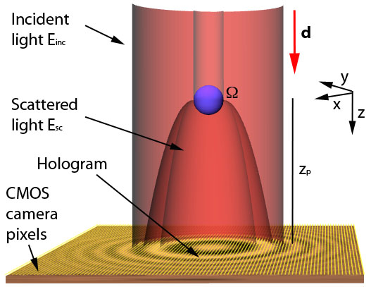
Figure 1: Schematic representation of in-line hologram formation. The incident light beam ${\mathbfcal E}_{inc}$ is scattered by the object $\Omega$. The resulting interference pattern ${\mathbfcal I}=|{\mathbfcal E}_{inc}+{\mathbfcal E}_{sc}|^{2}$ is recorded at a grid of CMOS camera pixels, forming the hologram. We consider here objects diameters in the range $10\,{\rm nm}$ - $2\,\mu$m ($1\,\mu$m = $10^{-6}{\rm m}$, $1$ nm = $10^{-9}{\rm m}$). Typical distances $z_{p}$ to the screen are about $5\,\mu$m. The screen covers an area $10\,\mu{\rm m}\times 10\,\mu{\rm m}$ and the CMOS grid step is $0.1\,\mu$m.

When the approximate location in the field of view is known, objects describable by simple parametrizations, such as spheres or rods, can be approximated from in-line holograms by fitting the parameters so that the difference between the synthetic holograms generated by them and measured hologram diminishes [22, 31, 34, 53]. For spherical particles, the scattered electric field is given explicitly by the Mie solution [22, 31]. Spheres and rods have also been handled through the discrete dipole approximation (DDA) [53]. The employed techniques are computationally intensive, though this drawback can be diminished while keeping the resolution by resorting to a smaller number of randomly distributed detectors [13].

To image scatterers without previous knowledge of their geometry, number and approximate location in the field of view, we may address more general optimization problems in which the design variable is the unknown domain. Different techniques differ in the way the objects are represented and deformed to decrease the value of the cost functional. When the number of scatterers is known, classical shape deformation along adequately chosen vector fields may be used [40, 45, 19]. However, this procedure does not allow for topological changes: the exact number of contours has to be known from the beginning [38]. Deformations inspired in level set methods, instead, allow to create and destroy contours during the process [16, 17, 38]. All these methods require an initial guess of the object contours to proceed. Topological derivative techniques provide such guesses without a priori information and do not require a specific parametrization of the objects [20]. They have been combined with both shape derivatives and level sets to approximate objects in a variety of aplications, such as flow studies and electric impedance tomography [10, 32]. Methods entirely built on topological field based approximations have been employed in acoustics, materials testing and electric impedance tomography [1, 6, 15, 20, 26, 43], for instance. The results may be refined by combining multiple frequencies [1], many directions [27] or by iteration [5]. They may require less iterations than level sets, though some previous calibration work is needed. Most practical implementations have used incident directions and detectors distributed over wide angle ranges, usually in 2D settings. When imaging with one light beam, and assuming that the electric field instead of the hologram was known, we showed that topological methods provide approximations of the 3D scatterers [7]. If the object permittivity is known and the objects size is small enough compared to the wavelength, these approximations may be improved by a combination of topological derivative techniques, blobby molecule fittings and a forward solver [7]. Here we tackle the inversion problem of recovering the 3D scatterers from the recorded hologram in two ways. A first possibility is to find a strategy to predict numerically the electric field from the recorded hologram and use this prediction as approximate data. This is done here employing topological methods, gradient optimization and Gaussian filtering. Alternatively, we may seek to optimize the holographic cost functional, which measures the deviation with respect to the recorded hologram. Combining topological and descent methods we succeed in approximating objects and their permittivities with no a priori knowledge, other than the ambient permittivity and the measured hologram. We observe that the initial reconstructions provided by both strategies are similar. However, the later one is more straightforward. Whether the first one may lead to more accurate approximations when iterated or combined with other techniques is a matter of study since other factors, such as the distance to the detectors and the size of the hologram, play a role too.

Our numerical approximations of the electric field pave the way to adapting to this framework techniques based on its knowledge developed for larger wavelengths. A wide variety of methods tracking permittivity variations have been introduced whose applicability in holography settings may be explored [6, 8, 9, 18, 37, 49, 51]. Qualitative techniques such as linear sampling [8, 3], as well as factorization and MUSIC methods [30, 3], have been analyzed when a much wider distribution of incident waves and observation points are employed. In holography settings, we must work with penetrable objects using only one incident wave and intensities measured at observation points located on a limited flat screen, for moderate to large dimensionless wavenumbers. When the optical properties of objects are unknown, we are able to infer them in an additional optimization step.

The paper is organized as follows. Section 2 provides a variational formulation of the inverse scattering problem in holography, assuming light polarized in the direction $x$ and neglecting the $y$,$z$ components of the electric field. With pure $x$ polarization, we see $y$ polarization at around a factor of $15$ lower intensity, both for single spheres and sets of two spheres. Such observations motivate the assumption. We consider here geometrical shapes typically adopted by bacteria and viruses, whose sizes are of a similar order or smaller than the wavelength. For simple arrangements, the polarization assumption we make is reasonable. As the geometrical configurations become more complex, enhanced scattering may require the use of the full vector Maxwell equations. The performance of the technique in the vectorial case is to be explored. Section 3 constructs initial approximations of the objects exploiting the topological derivative and energy associated to a functional quantifying the deviation between the hologram generated by any arbitrary shape at the recording screen and the hologram generated by the true object. Both are calculated using the incident light beam and an explicit adjoint field, which depends on the recorded hologram. Topological fields quantify the variations of a shape functional when creating or modifying objects in the ambient medium. Multiple and non convex objects can be handled, down to nanometer sizes, see Figures 2-4. As it is often the case in microscopy, working with one incident wave results here in a different resolution in planes orthogonal to the incidence direction and along the incidence direction. Whereas the shape and location of the objects are correctly represented in orthogonal slices, they may be shifted and elongated in the incidence direction, specially for small sizes. Elongation and loss of axial resolution are also present in traditional holographic reconstruction techniques based on numerical backpropagation [52]. For object sizes of the same order or smaller than the light wavelength, Section 4 explains how to reduce the offset and determine the number of object components by a topological derivative based iterative scheme. Moreover, we suggest strategies to combine these procedures with additional optimization with respect to the permittivity of the objects to determine it when unknown. We illustrate the horizontal and axial resolution of the technique studying the test cases of two objects with different permittivities located on the same $xy$ plane and two objects aligned along the incidence direction. By iteration, we are able to detect secondary objects with smaller contrast as well as objects screened by another scatterer aligned with them in the incidence direction, reducing in both cases the shift towards the screen in the objects position. We observe that a good approximation of the scatterers location is essential to improve the predictions of their parameters. Section 5 explores an alternative initialization procedure which might help to reduce the elongation in the incidence direction, using the hologram to produce approximations of the electric field at the recording screen. The idea is to seek real and imaginary values that minimize the error when compared to the recorded hologram. This is done by a gradient method starting from the explicit field scattered by objects fitted to the peaks of a rough initial topological energy. Gradient optimization is alternated with Gaussian filtering to smooth out local spikes. Section 6 summarizes our conclusions. Two final appendices compute the derivatives of the holography cost functional with respect to domains and coefficients and give explicit formulas for forward and adjoint fields in presence of penetrable spheres, which are useful to obtain the formulas for the topological derivatives and to lower the computational complexity in specific situations.

(a)                              (b)                              (c)

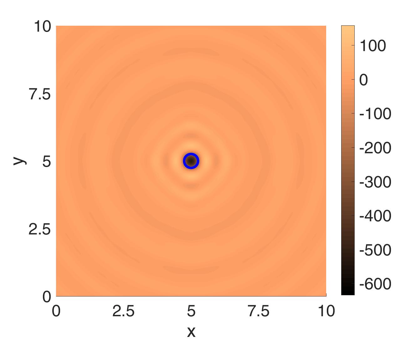
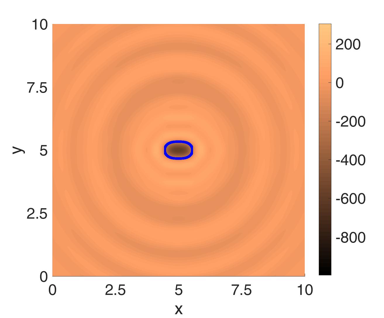
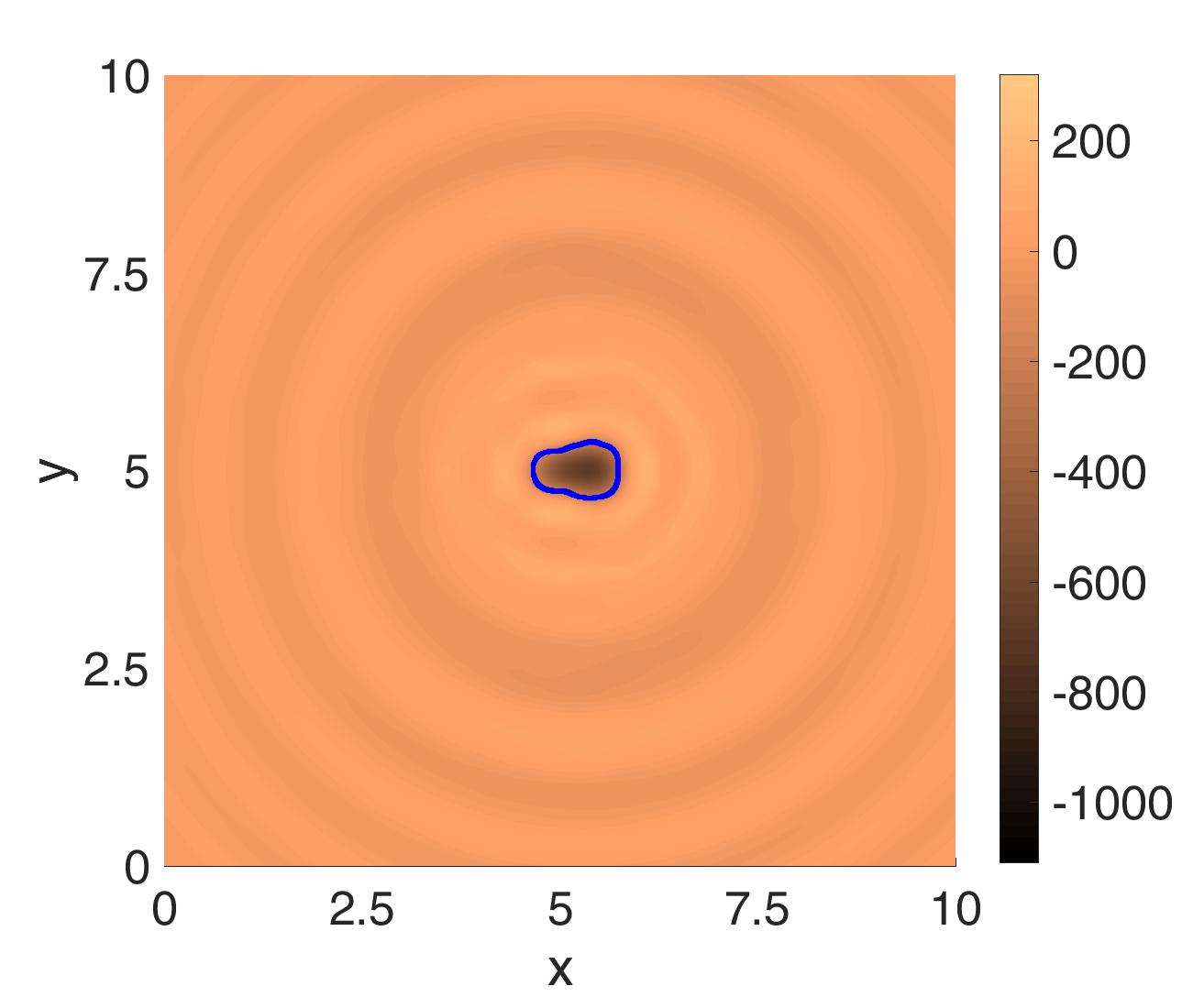
(d)                              (e)                              (f)

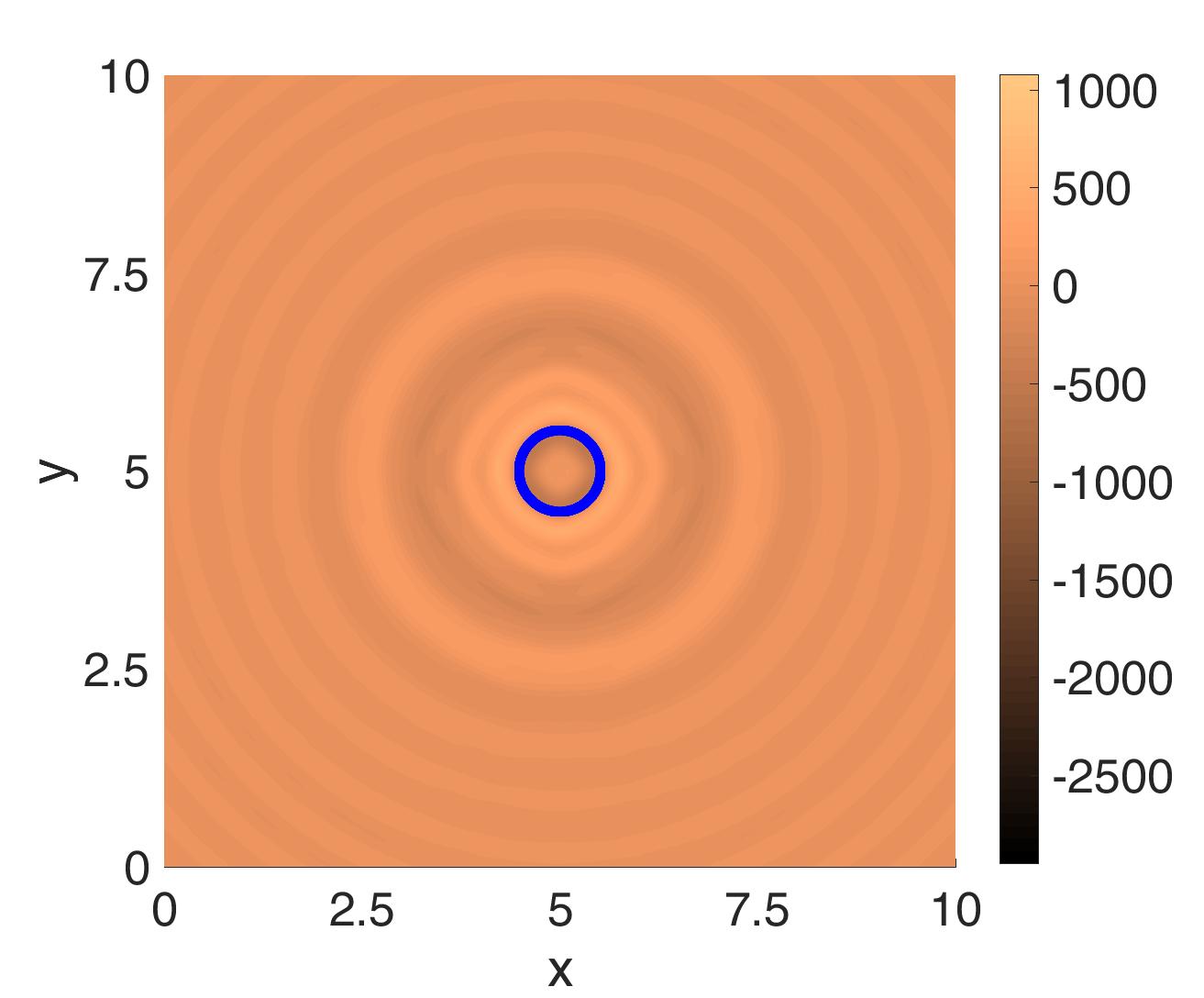
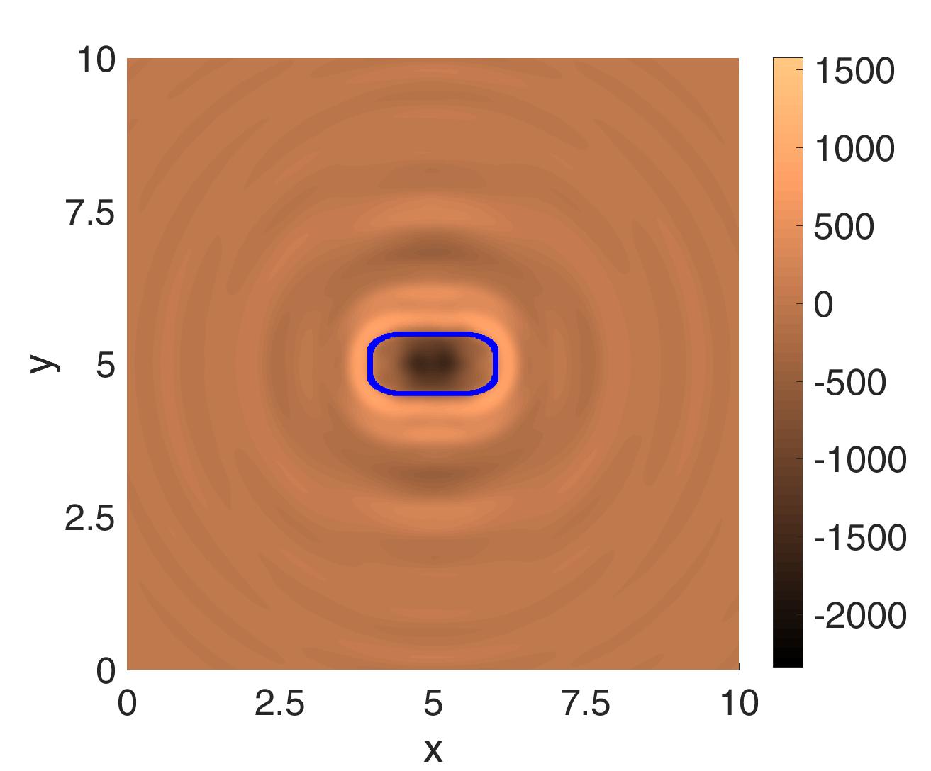
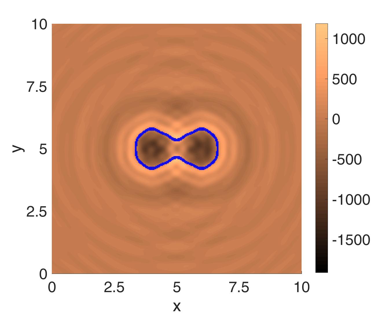
Figure 2: Slices $z=5$ of the topological derivatives for the holography cost functional (3), computed evaluating (8) with (11) and (15). For ${k}_{e}=12.6$ and ${k}_{i}=15.12$ (red light of wavelength $660\,{\rm nm}$): (a) Sphere of radius $0.25$ ($250\,{\rm nm}$, $1\,{\rm nm}=10^{-9}\ {\rm m}$), (b) Spherocylinder of maximum radius $0.25$ and length $1$, oriented along the $x$ axis, (c) Pear shaped object oriented along the $x$ axis, with maximum radius $0.25$. For ${k}_{e}=20.60$ and ${k}_{i}=24.79$ (violet light of wavelength $405$ nm): (d) Sphere of radius $0.5$. (e) Spherocylinder of maximum radius $0.5$ and length $2$, oriented along the $x$ axis. (d) Sand clock shaped object, with maximum radius $1$ and length $4$, oriented along the $x$ axis. The darkest regions represent the approximate shape. The true object borderline is superimposed. Objects are placed at the center of a box of size $10$ in the imaging setting represented in Figure 1. The distance to the screen and to the emitter is $5$ ($5\,\mu$m, $1\,\mu{\rm m}=10^{-6}\ {\rm m}$).

(a)                             (c)                              (e)

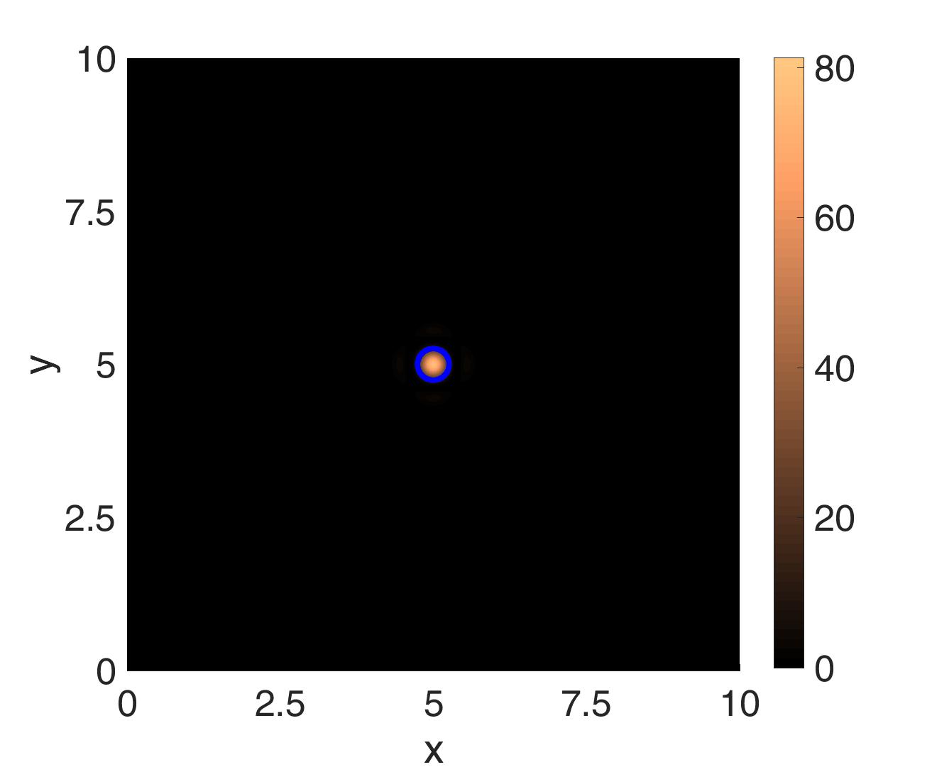
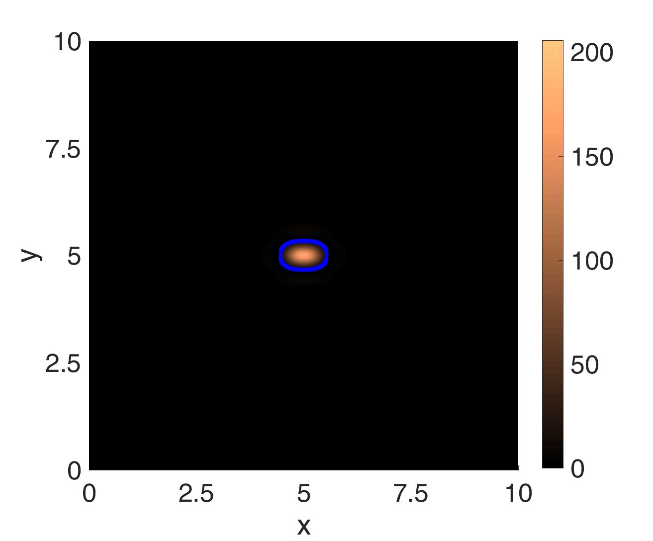
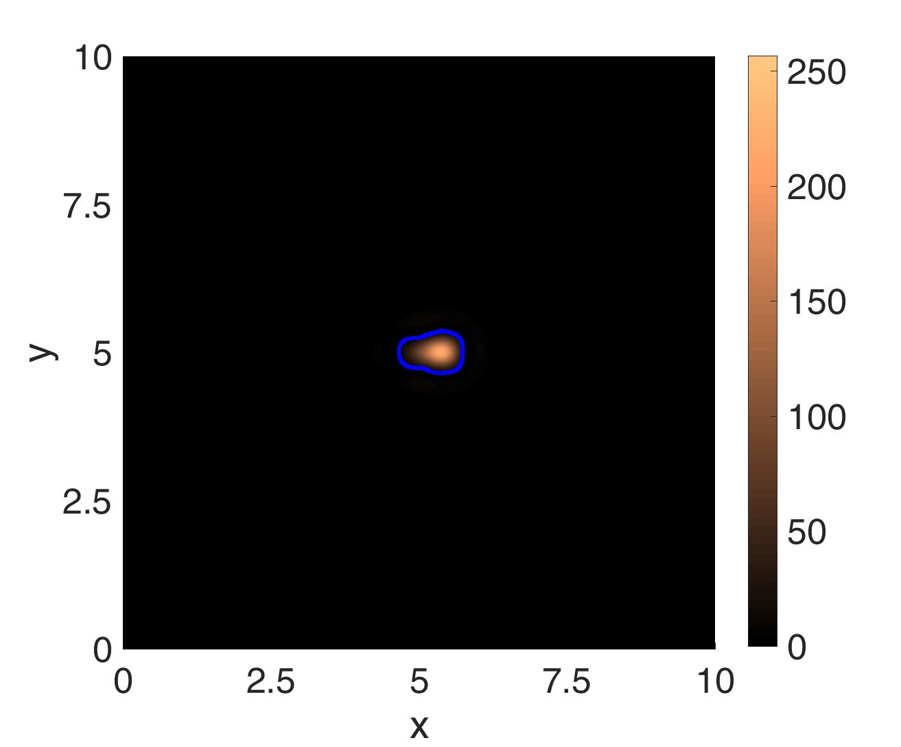
(b)                             (d)                              (f)

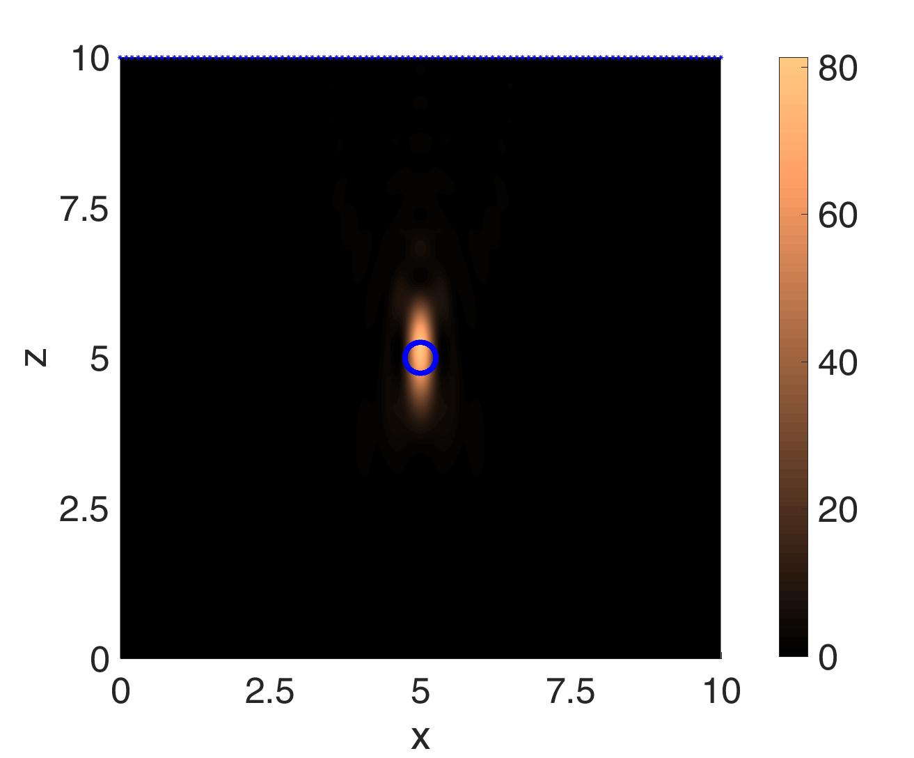
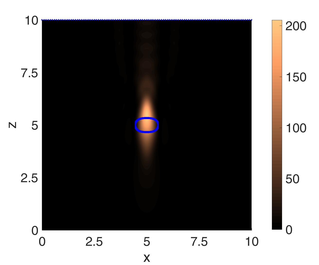
Figure 3: Slices $z=5$ and $y=5$ of the topological energies of the holography cost functional (3), given by (16) with (11) and (15) for the same objects and parameters considered in Fig. 2 (a)-(c). (a),(b) Sphere. (c),(d) Spherocylinder. (e),(f) Pear shaped object. The brightest spots represent the approximate objects. The true borderline is superimposed. Whereas the slices $z=5$ reproduce correct shapes and positions, the objects appear to be shifted and elongated in the $y=5$ slices.

(a)                                    (b)

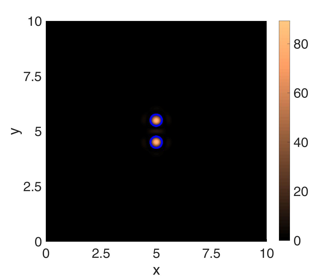
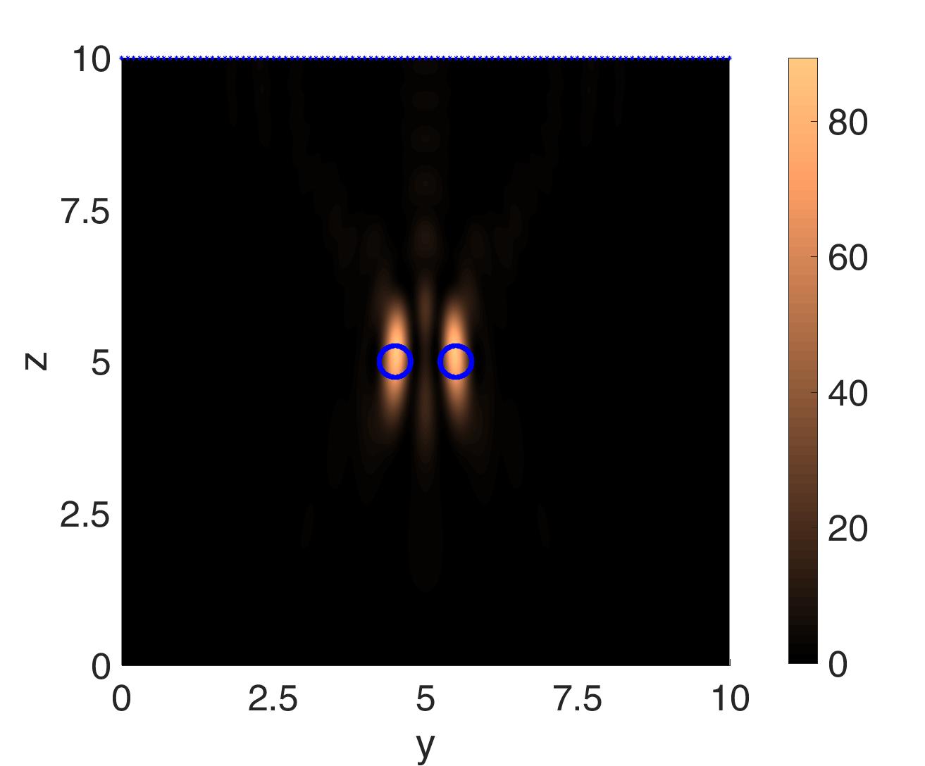
(c)                                    (d)

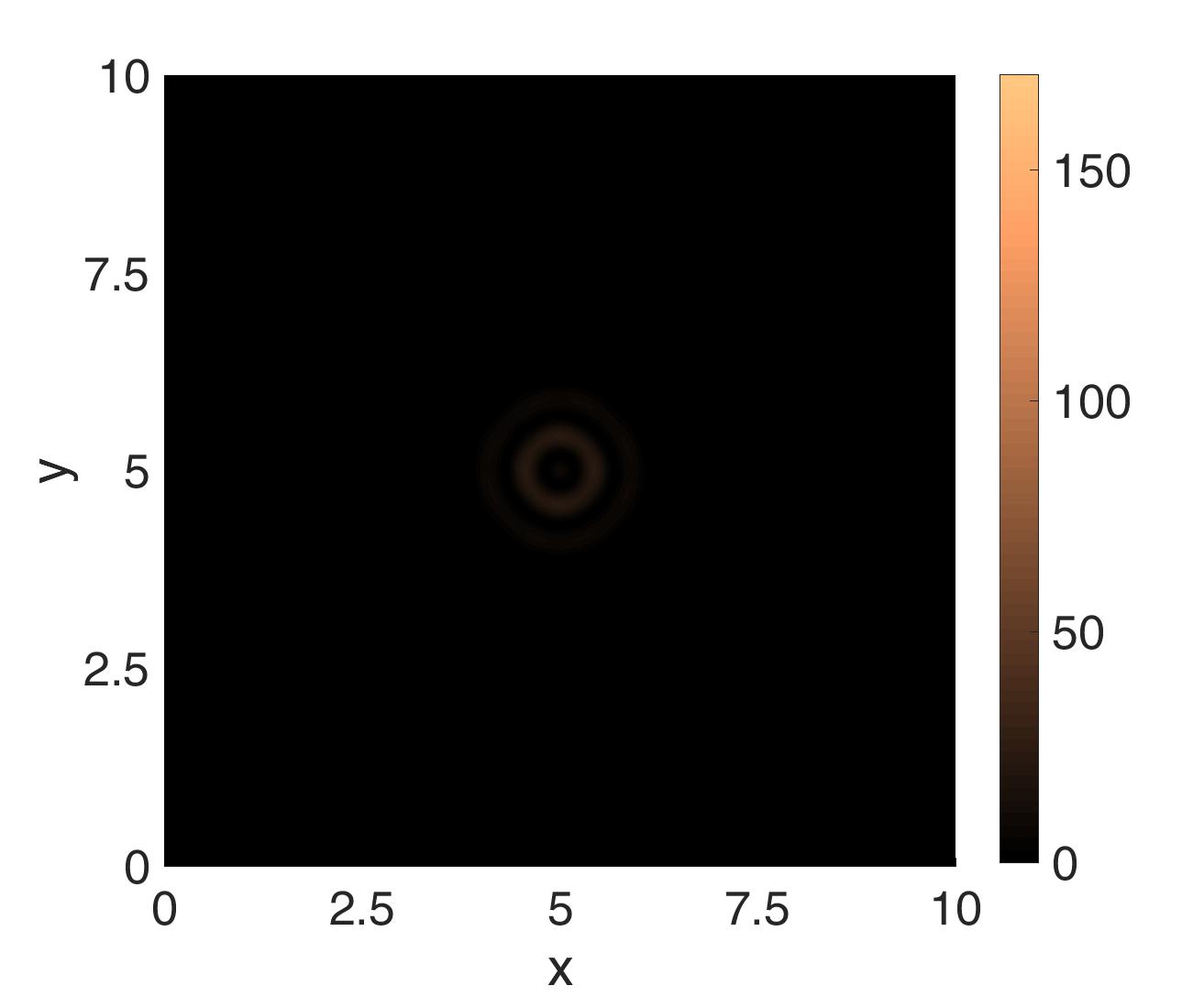
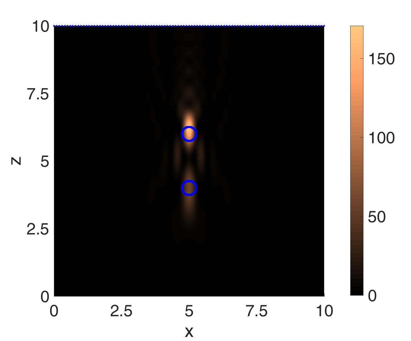
Figure 4: Slices $z=5$ and $x=5$ (resp. $y=5$) of the topological energies for the holography cost functional (3), computed evaluating (16) with (11) and (15) when ${k}_{e}=12.6$ and ${k}_{i}=15.12$. (a),(b) Two spheres of radius $0.25$ ($250$ nm), aligned along the $y$ axis and separated a distance $0.5$. (c),(d) Two spheres of radius $0.25$, aligned along the $z$ axis, located at $z=4$ and $z=6$. The borderline of the true objects is superimposed.

2 Variational formulation of the inverse holography problem

Electromagnetism equations for light have been used to fit real holograms to spheres and rods in references [31, 53], for instance. Ref. [31] exploits explicit Mie solutions of Maxwell’s equations whereas ref. [53] relies on discrete dipole approximations. For light polarized in the direction $x$ (resp. $y$), the component $x$ (resp. $y$) of the electric field is the relevant one. Since we work with polarized light, we reduce the Maxwell system to a single scalar wave equation for the relevant component.

In presence of a set of particles occupying a domain $\Omega$, part of the incident wave is transmitted inside the objects and the remaining portion is scattered. The evolution of the selected component

$${\mathcal{E}}(\mathbf{x},t):=\left\{\begin{array}[]{ll}{\mathcal{E}}_{inc}(\mathbf{x},t)+{\mathcal{E}}_{sc}(\mathbf{x},t),&\quad\mbox{$\mathbf{x}\in\mathbb{R}^{3}\setminus\overline{\Omega}$},\ \ t>0,\\ {\mathcal{E}}_{tr}(\mathbf{x},t),&\quad\mbox{$\mathbf{x}\in\Omega$},\ \ t>0,\end{array}\right.$$

is governed by the wave equation

(1) $$\varepsilon(\mathbf{x}){\mathcal{E}}_{tt}(\mathbf{x},t)-{\rm div}\left({1\over{\mu(\mathbf{x})}}\nabla{\mathcal{E}}(\mathbf{x},t)\right)=0,$$

where $\varepsilon$ represents the permittivity and $\mu$ the permeability. When the incident light is time-harmonic with frequency $\nu$, that is, ${\mathcal{E}}_{inc}(\mathbf{x},t)=\mbox{Re}[e^{-2\pi\imath\nu t}E_{inc}(\mathbf{x})],$ the resulting electric wave field $\mathcal{E}$ is time-harmonic too: ${\mathcal{E}}(\mathbf{x},t)=\mbox{Re}[e^{-2\pi\imath\nu t}E(\mathbf{x})]$, with (complex) amplitude $E(\mathbf{x})$.

The electric field $E_{sc}$ scattered by the objects $\Omega$ generating an hologram ${\mathcal{I}}$ satisfies

(2) $$|E(\mathbf{x}_{j})|^{2}=|E_{sc}(\mathbf{x}_{j})+E_{inc}(\mathbf{x}_{j})|^{2}={\mathcal{I}}(\mathbf{x}_{j}),\quad j=1,\ldots,N,$$

at the detectors where the hologram ${\mathcal{I}}$ is recorded. Finding the objects whose scattered electric field satisfies (2) is the inverse holography problem, which can be recast as an optimization problem: Find regions $\Omega\subset{\mathbb{R}}^{3}$ minimizing

(3) $$J(\mathbb{R}^{3}\setminus\overline{\Omega})={1\over 2}\sum_{j=1}^{N}||E(\mathbf{x}_{j})|^{2}-{\mathcal{I}}(\mathbf{x}_{j})|^{2},$$

where $E=E_{sc}+E_{inc}$ is the (complex) amplitude of the total electric field in presence of $\Omega$ and ${\mathcal{I}}$ is the measured hologram. The true objects are a global minimum at which functional (3) vanishes.

This formulation assumes the parameters characterizing the optical properties of the objects known. When unknown, we may consider (3) a functional depending on two variables $J(\mathbb{R}^{3}\setminus\overline{\Omega},k_{i})$ and seek regions $\Omega\subset{\mathbb{R}}^{3}$ and parameter functions $k_{i}:\Omega\rightarrow{\mathbb{R}}^{+}$ minimizing $J(\mathbb{R}^{3}\setminus\overline{\Omega},k_{i})$ in presence of objects $\Omega$ with wavenumber $k_{i}$, $k_{i}=k_{i}(\nu,\mu,\varepsilon)$. When the variations in the wavenumber are not abrupt enough, we may fix a region of interest $\Omega$, consider (3) as a functional $J(k_{i})$ and seek coefficient functions $k_{i}:\Omega\rightarrow{\mathbb{R}}^{+}$ minimizing $J(k_{i})$. Here, we will mostly work with $J(\mathbb{R}^{3}\setminus\overline{\Omega}),$ and occasionally with $J(\mathbb{R}^{3}\setminus\overline{\Omega},k_{i})$, since it is usually more efficient to track abrupt variations in the wavenumber which would define objects and then study wavenumber variations inside them if required [6].

The equations governing $E$ act as a constraint in this optimization problem. Nondimensionalizing, we may take $E$ to be a dimensionless amplitude obeying

(4) $$\left\{\begin{array}[]{ll}\Delta_{\mathbf{x}}E+{k}_{e}^{2}E=0,&\quad\mbox{in $\mathbb{R}^{3}\setminus\overline{\Omega}$},\\ \Delta_{\mathbf{x}}E+{k}_{i}^{2}E=0,&\quad\mbox{in $\Omega$},\\ E^{-}=E^{+},&\quad\mbox{on $\partial\Omega$},\\ \beta(\partial_{\mathbf{n}}E)^{-}=(\partial_{\mathbf{n}}E)^{+},&\quad\mbox{on $\partial\Omega$},\\ \displaystyle\lim_{r:=|\mathbf{x}|\to\infty}r\big{(}\partial_{r}(E-E_{inc})-\imath{k}_{e}(E-E_{inc})\big{)}=0.\end{array}\right.$$

The incident wave is a plane wave in the direction $\hat{\bf d}=(0,0,1)$, that is, $E_{inc}(\mathbf{x})=E_{inc}(x,y,z)=e^{\imath{k}_{e}z}$. The detectors are located at the screen $z=z_{0}$, see Figure 1. The superscripts “$+$” and “$-$” denote limits from the exterior and the interior of $\Omega$ respectively. The symbol $\partial_{\mathbf{n}}$ stands for normal derivative. The condition at infinity is the standard Sommerfeld radiation condition allowing only outgoing waves, where $\partial_{r}$ represents radial derivatives.

Dimensions are restored by setting $\mathbf{\tilde{x}}=\mathbf{x}L$, $\tilde{\Omega}=\Omega L$, $\tilde{E}(\mathbf{\tilde{x}})=E_{0}E(\mathbf{x}L)$, $\tilde{E}_{inc}(\mathbf{\tilde{x}})=E_{0}E_{inc}(\mathbf{x}L)=E_{0}e^{\imath\tilde{k}_{e}\hat{\mathbf{d}}\cdot\mathbf{\tilde{x}}},$ where $L$ is a reference length unit, $E_{0}$ a reference field, and

(5) $$\tilde{k}_{e}:=k_{e}/L,\qquad\tilde{k}_{i}:=k_{i}/L.$$

The wavenumbers $\tilde{k}_{e}$ and $\tilde{k}_{i}$ are usually expressed in terms of refractive indexes $n_{i},n_{e}$ (ratio of the speed of light in the vacuum to the speed in a particular medium):

(6) $$\tilde{k}_{e}=\frac{2\pi\nu}{c_{e}}=\frac{2\pi}{\lambda}n_{e},\qquad\tilde{k}_{i}=\frac{2\pi\nu}{c_{i}}=\frac{2\pi}{\lambda}n_{i},$$

where $\lambda$ is the wavelength of the employed light in the vacuum. Assuming the permittivity $\varepsilon$ and permeability $\mu$ to be constant in the ambient medium and in the scatterers, the local wave speeds are $c_{e}={1\over\sqrt{\mu_{e}\varepsilon_{e}}}$ for the medium and $c_{i}={1\over\sqrt{\mu_{i}\varepsilon_{i}}}$ for the objects, with $\mu_{e}=\beta\mu_{i}.$ For biological samples $\beta\sim 1$. We will set $\beta=1$ in our numerical tests.

For arbitrary shapes $\Omega$ and constant coefficients, one can solve an integral reformulation of any boundary interior or exterior problem for Helmholtz equations. Here we make use of an integral representation of the solution in the exterior domain and deduce a non symmetric formulation which combines boundary elements (BEM) and finite elements (FEM) [7, 28, 41]. We discretize this formulation by means of piecewise constant boundary elements and continuous $\mathbb{P}1$ finite elements, so that our solving scheme has order one. This method allows us to generate the synthetic holograms employed here for the reconstructions. Also, notice that for isolated spherical objects $\Omega$ and constant wave speeds both in the medium and in the objects, the scalar system (4) admits explicit solutions, expressed as series expansions in terms of spherical harmonics [35, 47], see Appendix B. This is a scalar version of the Mie solutions for the vector Maxwell equations [2, 44].

To address the general optimization problem for (3) without a priori information on the number of scattering objects, their geometry and approximate location we need to calculate the derivatives of the holography cost functional with respect to domains and coefficients. This is done in Appendix A.

3 Initial predictions of shapes from recorded holograms

Topological methods provide a way to quantify variations of shape functionals due to the presence of objects, which allows us to construct guesses of objects from the knowledge of the hologram and the optical properties of the ambient medium. The idea is the following. Consider a functional $J({\cal R})$, defined in a region ${\cal R}\subset\mathbb{R}^{3}$. Removing from it a ball of radius $\varepsilon$ centered about $\mathbf{x}$, the expansion

(7) $$J({\cal R}\setminus\overline{B_{\varepsilon}(\mathbf{x})})=J({\cal R})+{4\over 3}\pi\varepsilon^{3}D_{T}(\mathbf{x},{\cal R})+o(\varepsilon^{3}),\qquad\varepsilon\to 0,$$

holds. $D_{T}(\mathbf{x},{\cal R})$ is the topological derivative of the functional at ${\mathbf{x}}$. As explained in Appendix A, it measures the variation of the functional when an object is placed at $\mathbf{x}$ [46] and it is used to localize abrupt changes. If $D_{T}(\mathbf{x},{\cal R})<0$, then $J({\cal R}\setminus\overline{B_{\varepsilon}(\mathbf{x})})<J({\cal R})$ for $\varepsilon>0$ small. Therefore, when we locate objects in regions where the topological derivative takes large negative values, the functional is expected to diminish [20]. In this way, we are able to predict the number, location and size of the scatterers.

Evaluating the topological derivative at a point using expansion (7) is too expensive for practical purposes. Instead, we use an expression in terms of adjoint and forward fields, see Appendix A for a derivation of these formulas and technical details. When we have no information on the object, we calculate $D_{T}(\mathbf{x},\mathbb{R}^{3})$ by means of the explicit formula:

(8) $$\hskip 8.53581ptD_{T}(\mathbf{x},\mathbb{R}^{3})={\rm Re}\left[3{1-\beta\over 2+\beta}\nabla E(\mathbf{x})\!\cdot\!\nabla\overline{P}(\mathbf{x})\!+\!(\beta k_{i}^{2}-k_{e}^{2})E(\mathbf{x})\overline{P}(\mathbf{x})\right],\;\mathbf{x}\in\mathbb{R}^{3},$$

where $E$ is the solution of the forward problem:

(11) $$\left\{\begin{array}[]{ll}\Delta E+{k}_{e}^{2}E=0&\quad\mbox{in ${\mathbb{R}}^{3}$},\\ \displaystyle\lim_{r\to\infty}r\big{(}\partial_{r}(E-E_{inc})-\imath{k}_{e}(E-E_{inc})\big{)}=0,\end{array}\right.$$

and $\overline{P}$ is the solution of the conjugate adjoint problem:

(14) $$\left\{\begin{array}[]{ll}\Delta\overline{P}+{k}_{e}^{2}\overline{P}=2\sum_{j=1}^{N}({\mathcal{I}}-|E|^{2})\overline{E}\,\delta_{{\mathbf{x}}_{j}}&\quad\mbox{in ${\mathbb{R}}^{3}$},\\ \displaystyle\lim_{r\to\infty}r\big{(}\partial_{r}\overline{P}-\imath{k}_{e}\overline{P}\big{)}=0,\end{array}\right.$$

$\delta_{\mathbf{x}_{j}}$ being Dirac masses supported at the receptors. For an incident plane wave, $E=E_{inc}$ and $\overline{P}$ is given by:

(15) $$\overline{P}({\mathbf{x}})=-\sum_{j=1}^{N}{e^{\imath{k}_{e}|{\mathbf{x}}-{\mathbf{x}_{j}}|}\over 4\pi|{\mathbf{x}}-{\mathbf{x}_{j}}|}[2({\mathcal{I}}({\mathbf{x}_{j}})-|E({\mathbf{x}_{j}})|^{2})\overline{E}(\mathbf{x}_{j})].$$

When $\beta\sim 1$, the gradients disappear from (8) and $D_{T}(\mathbf{x},\mathbb{R}^{3})=(k_{i}^{2}-k_{e}^{2})E(\mathbf{x})\overline{P}(\mathbf{x}).$

The topological energy is a companion field of the topological derivative which has the ability of canceling oscillations as $k_{e}$ or the number of objects grow [15]:

(16) $$E_{T}(\mathbf{x},{\mathbb{R}}^{3})=|E(\mathbf{x})|^{2}|{P}(\mathbf{x})|^{2}.$$

Peaks of the topological energy indicate the location of objects. Plotting the topological derivatives instead, the regions where large negative values are attained represent object shapes. Our simulations show an effect often observed in microscopy: very different resolution in planes orthogonal to the incidence direction of the light beam when compared with resolution along the incidence direction. Whereas $xy$ slices capture correct positions and shapes, the objects appear to be elongated and shifted in the incidence direction, see Figures 2-4.

The technique is tested in the imaging setting represented in Figure 1 with light of wavelength $660\,{\rm nm}$ (red) and $405\,{\rm nm}$ (violet). The light emitter is placed at $z=0$. A hologram recording screen of size $10\mu{\rm m}\times 10\mu{\rm m}$ is located at $z=10\mu{\rm m}$. The problem is nondimensionalized choosing $L=1\,\mu$m, representative of the average object size considered. The original permittivities are typical of biological media and $\beta=1$. Many bacteria display spherical or rod-like shapes and their size lies in the range of a few microns. They adopt the forms depicted in Fig 2(c) and Fig 2(f) when they are moving or dividing. Viruses also adopt simple geometrical shapes, with typical sizes ranges from $500$ nm down to $30$ nm. Here, the data are synthetic holograms generated solving the forward problem (4) for the true objects by BEM-FEM, as described in [7, 28, 41]. Figure 5 displays some of the synthetic holograms ${\cal I}=|E_{sc}+E_{inc}|^{2}$ used in the holography cost functional (3) and for the calculation of the adjoint (15). For specific objects, we have checked that holograms generated by BEM-FEM, DDA [50] and/or the series solutions in Appendix B agree. The relative error in the difference is of order $10^{-1}$ for our typical choices of the wavelength and the mesh size. The numerical error can be considered as noise; indeed, we have checked that we do not commit any numerical crime by seeing that the introduction of random noise in the data does not lead to significant change in our reconstructions. Topological methods have been shown to be very robust to the presence of noise.

(a)                           (b)                            (c)

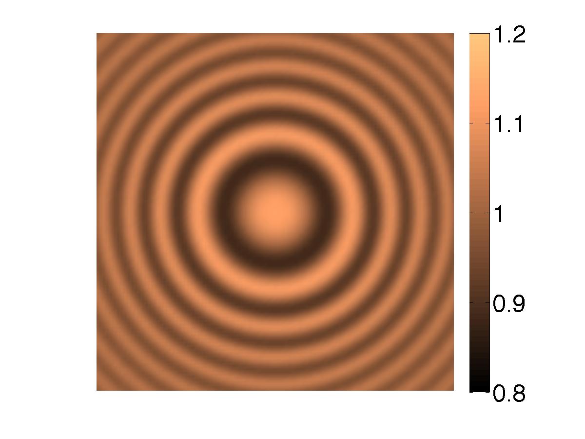
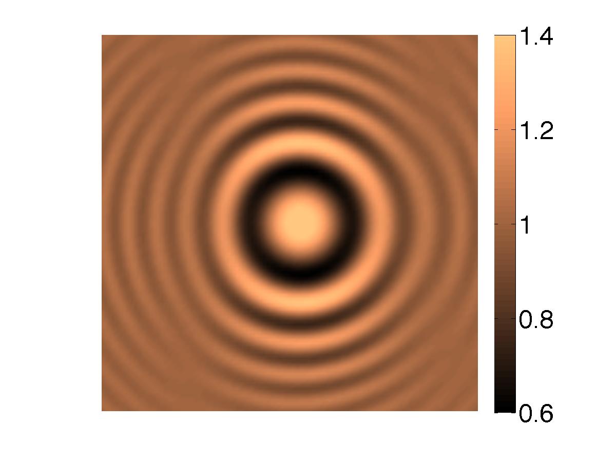
(d)                           (e)

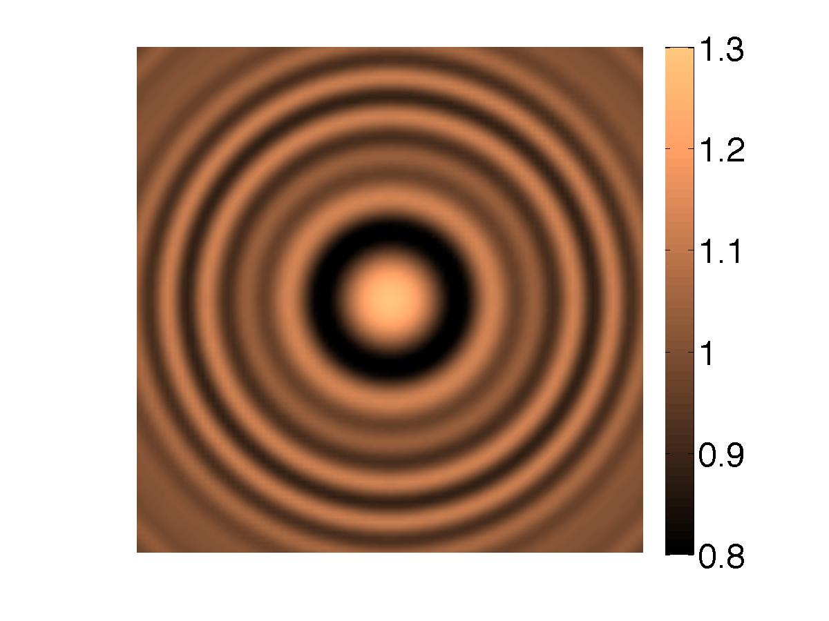
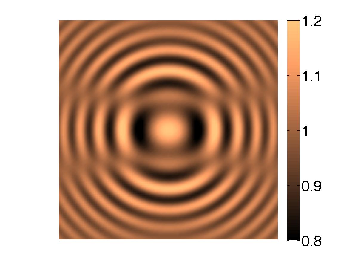
Figure 5: Synthetic holograms ${\cal I}=|E_{sc}+E_{inc}|^{2}$ for the shapes considered in Figures 3-4: (a) Sphere, (b) Spherocylinder, (c) Pear-shaped object, (d) Two spheres of the same material, aligned along the $z$ axis, (e) Two spheres of the same material, aligned along the $y$ axis.

Figure 6: Procedure to recover objects from the hologram in our imaging setting, for the cost functional (3) and sizes similar to or smaller than the wavelength.

(a)                              (c)                              (e)

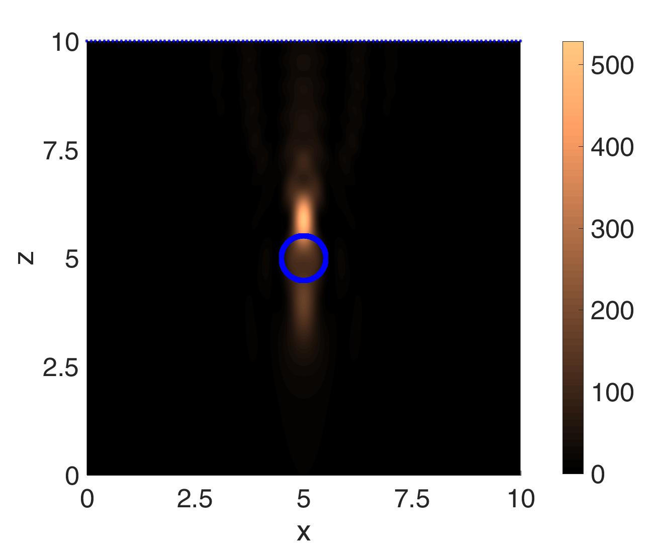
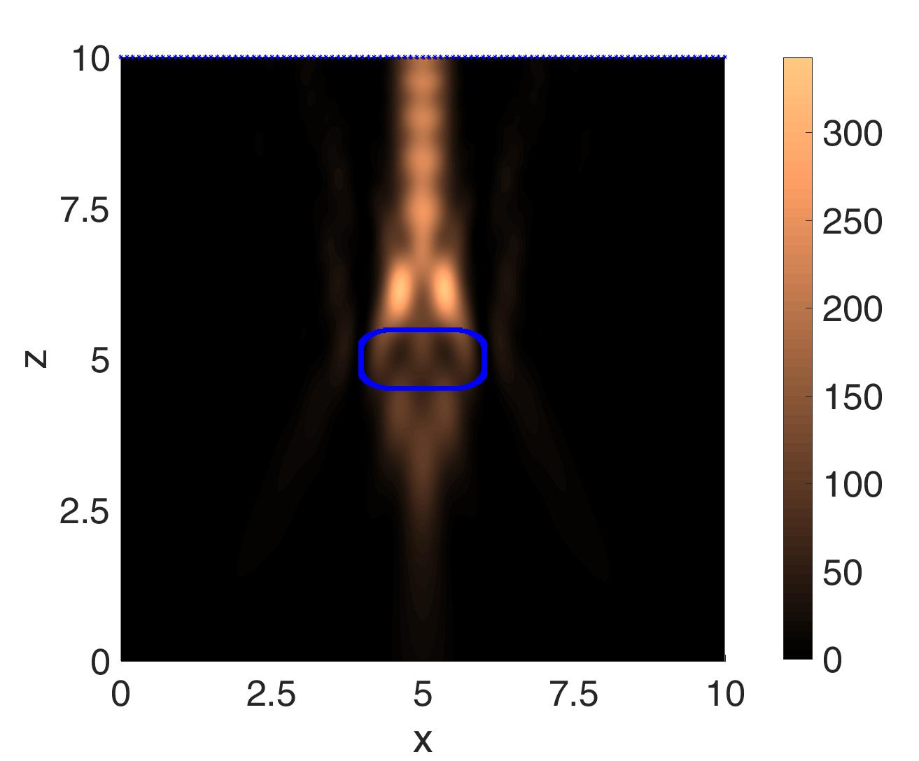
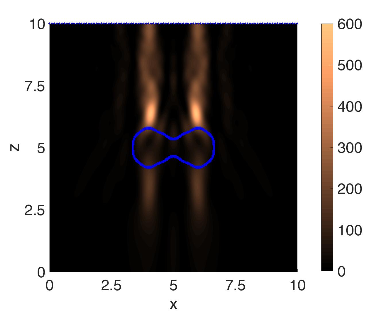
(b)                              (d)                              (f)

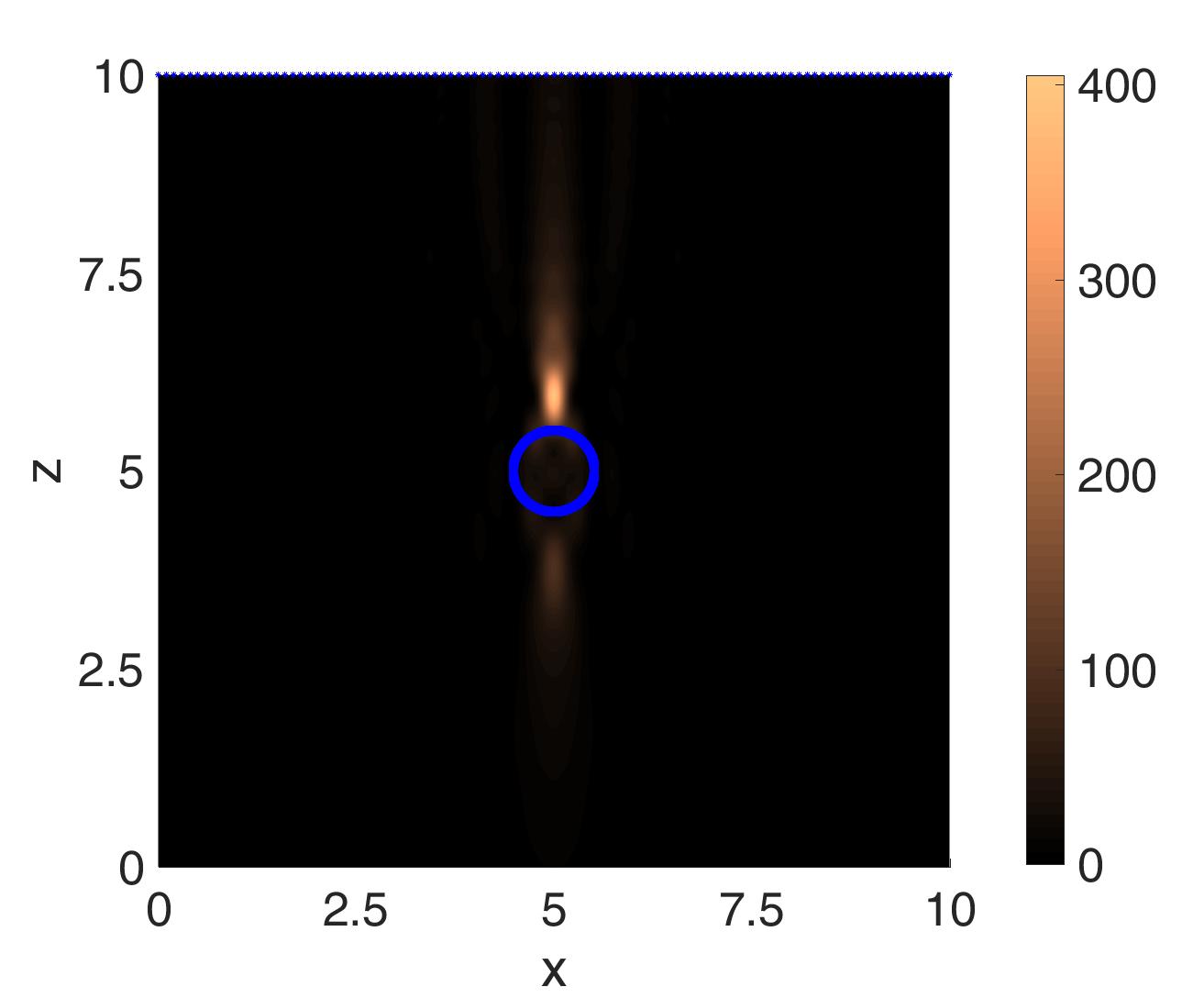
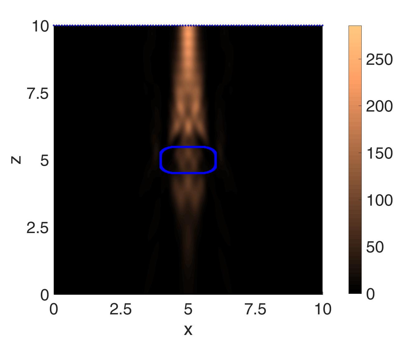
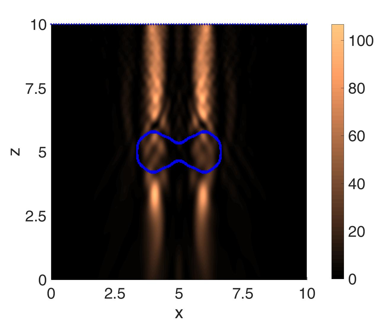
Figure 7: Slices $y=5$ of the topological energies for the holography cost functional (3) computed evaluating (16) with (11) and (15) for the objects considered in Fig. 2 (d)-(f). (a),(b) Sphere. (c),(d) Spherocylinder. (e),(f) Sand clock shaped object. The top row corresponds to ${k}_{e}=12.6$ and ${k}_{i}=15.12$. The bottom row corresponds to ${k}_{e}=20.60$ and ${k}_{i}=24.79$.

Then, a simple strategy to define an initial guess $\Omega^{(0)}$ for the scatterer is

(17) $$\Omega^{(0)}:=\{{\bf x}\in{\mathbb{R}}^{3}\,|\,E_{T}({\bf x},{\mathbb{R}}^{3})\geq C_{0}\}$$

where $C_{0}$ is a positive constant, chosen so that $J({\mathbb{R}}^{3}\setminus\overline{\Omega}^{(0)})<J({\mathbb{R}}^{3})$. Otherwise, we increase the constant $C_{0}$. The process is sketched in Figure 6. Alternatively, we might set $\Omega^{(0)}:=\{{\bf x}\in{\mathbb{R}}^{3}\,|\,D_{T}({\bf x},{\mathbb{R}}^{3})\leq-C_{0}\}.$ In our tests, initialization (17) is usually easier to implement and reduces the shift towards the screen in the object location.

Notice that neither the definition of the topological energy (16) nor the analytical expressions for the forward and adjoint fields (11), (14), (15) depend on ${k}_{i}$ and $\beta$. Therefore, formula (17) provides a first approximation to the objects without knowing their optical properties beforehand. For biological samples $\beta\sim 1$ and the gradient term in expression (8) disappears. In consequence, the function ${\rm Re}[E(\mathbf{x})\overline{P}(\mathbf{x})]$ may also yield a guess of the objects ignoring the variations of ${k}_{i}$.

We have tried sizes in the range $10$ nm - $1\,\mu$m with similar results. However, the behavior of the topological fields change as the wavelength diminishes and the size of the object grows, a phenomenon that is still not well understood in spite of recent theoretical work [27]. Whereas the $xy$ slices still provide information on the shape, as shown in Fig. 2 (d)-(f), the peaks of the topological fields begin to concentrate in the illuminated and the dark side of the boundary in the incidence direction. Figure 7 illustrates the transition to this new behavior. Once it takes place, as in Fig. 7(f), this marks the location $[z_{1},z_{2}]$ of the object in the direction $z$ reducing the offset and loss of axial resolution. The shape is reconstructed plotting slices of the topological fields for values $z=z^{\prime}$ in that range $[z_{1},z_{2}]$. Bright areas in such slices reproduce the true shape and the object is approximated by gluing them together, see reference [7] for details.

In the next sections, we will restrict our study to situations in which the dimensionless wavenumbers $k_{i}$, $k_{e},$ are not large enough to reach this transition regime (the wavelength is large enough compared to the object size), so that iterative refinements to correct the offset, the number of objects and their parameters may be developed.

4 Geometry and parameter correction

The approximations to the scatterers obtained in Section 3 can be sharpened by an iterative procedure for small enough sizes, depending on the wavelength. We consider here the test problem of approximating two objects whose permittivities may be known or unknown, equal or different. We focus on two cases to clarify axial and horizontal resolution: two similar spheres aligned along the incidence direction and two spheres in an orthogonal plane with different permittivities in each sphere.

Consider the configurations with multiple balls along the $z$ axis in Figure 4(d). Using expression (17) we define an approximation $\Omega^{(0)}$ to the scatterers. We may take $C_{0}=\alpha_{0}\max_{{\bf x}\in\mathcal{R}_{obs}}E_{T}(\mathbf{x},\mathbb{R}^{3}),$ where $0<\alpha_{0}<1$ and $\mathcal{R}_{obs}$ is the region where we are looking for objects. However, depending on the value of $\alpha_{0}$ we are left with one or two, or more, elongated objects. Let us fix a value $\alpha_{0}$ for which only the upper object, the one closer to the screen is detected. The corresponding shape $\Omega^{(0)}$ is elongated along the $z$ axis. This guess $\Omega^{(0)}$ may improve updating the topological derivative field to consider its presence. A new approximation $\Omega^{(1)}$ is constructed from $\Omega^{(0)}$ following the iterative scheme:

(18) $$\Omega^{(n+1)}:=\{{\bf x}\in\Omega^{(n)}\,|\,D_{T}({\bf x},{\mathbb{R}}^{3}\setminus\overline{\Omega^{(n)}},k_{i})<c_{n+1}\}$$

$$\hskip 28.45274pt\cup\,\{{\bf x}\in\mathbb{R}^{3}\setminus\overline{\Omega^{(n)}}\,|\,D_{T}({\bf x},{\mathbb{R}}^{3}\setminus\overline{\Omega^{(n)}},k_{i})<-C_{n+1}\},$$

see Figure 8(a). For $\beta\sim 1$, the topological derivative is given by

(19) $$\hskip 8.53581ptD_{T}(\mathbf{x},\mathbb{R}^{3}\setminus\overline{\Omega^{(n)}},k_{i})={\rm Re}\left[(k_{i}^{2}-k_{e}^{2})E_{n}(\mathbf{x})\overline{P}_{n}(\mathbf{x})\right],\qquad\mathbf{x}\in\mathbb{R}^{3},$$

where the forward field $E_{n}$ is a solution of (4) with object $\Omega^{(n)}$ and the conjugate adjoint field $\overline{P}_{n}$ obeys

(25) $$\left\{\begin{array}[]{ll}\Delta\overline{P}_{n}+{k}_{e}^{2}\overline{P}_{n}=2\sum_{j=1}^{N}({\mathcal{I}}-|E_{n}|^{2})\overline{E}_{n}\delta_{{\mathbf{x}}_{j}}&\quad\mbox{in ${\mathbb{R}}^{3}\setminus\overline{\Omega^{(n)}}$},\\ \Delta\overline{P}_{n}+{k}_{i}^{2}\overline{P}_{n}=0,&\quad\mbox{in $\Omega^{(n)}$},\\ \overline{P}_{n}^{-}=\overline{P}_{n}^{+},&\quad\mbox{on $\partial\Omega^{(n)}$},\\ \beta\partial_{\mathbf{n}}\overline{P}_{n}^{-}=\partial_{\mathbf{n}}\overline{P}_{n}^{+},&\quad\mbox{on $\partial\Omega^{(n)}$},\\ \displaystyle\lim_{r\to\infty}r\big{(}\partial_{r}\overline{P}_{n}-\imath{k}_{e}\overline{P}_{n}\big{)}=0.\end{array}\right.$$

The positive constants $C_{n+1}$, $c_{n+1}$ in (18) are selected to ensure a decrease in the shape functional: $J({\mathbb{R}}^{3}\setminus\overline{\Omega^{(n+1)}})<J({\mathbb{R}}^{3}\setminus\overline{\Omega^{(n)}})$. Notice that for $\mathbf{x}\notin\Omega$ expansion (7) holds and the cost functional decreases adding to $\Omega$ points of negative topological derivative. On the contrary, for $\mathbf{x}\in\Omega$ we have $J((\mathbb{R}^{3}\setminus\overline{\Omega})\cup B_{\varepsilon})=J(\mathbb{R}^{3}\setminus\overline{\Omega})-{4\over 3}\pi\varepsilon^{3}D_{T}(\mathbf{x},\mathbb{R}^{3}\setminus\overline{\Omega})+o(\varepsilon^{3})$ and we must remove from $\Omega$ points with positive topological derivatives to decrease.

The approximations $\Omega^{(n)}$ provided by (17) or (18) have irregular shapes. To define their boundaries, we may fit starshaped parametrizations to each component, or adjust surfaces employing blobby molecules. This later approach, combined with BEM-FEM to evaluate forward and adjoint fields for $\Omega^{(n)}$ was taken in Ref. [7] for a different functional. Alternatively, one can use discrete dipole approximations that just need a discretized representation of objects [53]. We resort here to blobbly molecule fitting and the previously described non symmetric BEM-FEM scheme [7, 28, 41].

(a)                                                (b)

Figure 8: Procedure to sharpen the approximate scatterers for cost functional (3): (a) Keeping arbitrary shapes and computing the adjoint and forward fields by BEM-FEM. (b) When we are only interested in the number of objects and their position, we may reduce the computational complexity by an intermediate computation with spheres.

When we are only interested in determining the number of objects and their location, we may reduce the computational complexity by fitting balls $\hat{\Omega}^{(n)}$ to the current approximation $\Omega^{(n)}$ and setting

(26) $$\Omega^{(n+1)}:=\{{\bf x}\in\hat{\Omega}^{(n)}\,|\,D_{T}({\bf x},{\mathbb{R}}^{3}\setminus\overline{\hat{\Omega}^{(n)}},k_{i})<c_{n+1}\}$$

$$\hskip 28.45274pt\cup\,\{{\bf x}\in\mathbb{R}^{3}\setminus\overline{\hat{\Omega}^{(n)}}\,|\,D_{T}({\bf x},{\mathbb{R}}^{3}\setminus\overline{\hat{\Omega}^{(n)}},k_{i})<-C_{n+1}\},$$

Here, $D_{T}({\bf x},{\mathbb{R}}^{3}\setminus\overline{\hat{\Omega}^{(n)}},k_{i})$ may be evaluated solving the forward and adjoint problems (4), (25) for $\hat{\Omega}^{(n)}$ using the expansions in Appendix B. We can iterate the procedure fitting spheres $\hat{\Omega}^{(n+1)}$ to the components of $\Omega^{(n+1)}$ defined by (26) again. This is done by centering them at points where the minimum value of the topological derivative is attained and chosing as diameter of each component the smallest diameter in the three space directions. The procedure is summarized in Fig. 8(b).

We have treated the configuration in Figure 4(d) in both ways. Figure 9(a) plots the slice $y=5$ of the topological derivative $D_{T}({\bf x},\mathbb{R}^{3})$. Notice that only the object closer to the screen is clearly distinguished. Let us first apply the strategy in Fig. 8(b). Figure 9(b) displays the slice $y=5$ of the topological derivative $D_{T}({\bf x},{\mathbb{R}}^{3}\setminus\overline{\hat{\Omega}^{(0)}},k_{i})$ when $\hat{\Omega}^{(0)}$ is the sphere represented by a thin cyan contour in Figure 9(b), which has been fitted to $\Omega^{(0)}$ defined by (17). The two thicker solid blue contours correspond to the true objects. Following the rule (26), the updated object $\Omega^{(1)}$ should loose points in the upper half, where the topological derivative becomes positive and large, and gain neighboring points below the lower half, where the topological derivative becomes negative and large. Moreover, an additional prominent region where large negative values are attained is identified. Fitting two balls to $\Omega^{(1)}$ we obtain $\hat{\Omega}^{(1)}$ represented by the two dotted yellow lines, which we use to construct a new object $\Omega^{(2)}$ defined by (26), improving the position of the component placed farther from the screen. Instead, if we iterate with the procedure described in Fig. 8(a), keeping the approximations $\Omega^{(n)}$, $n=0,1,$ defined by (17)-(18) and calculating $D_{T}(\mathbf{x},\Omega^{(n)})$ by BEM-FEM, we also see the second object appear and the position improves, but the shapes remain elongated in the $z$ direction. Shapes in $xy$ slices are correct though.

(a)                                                     (b)

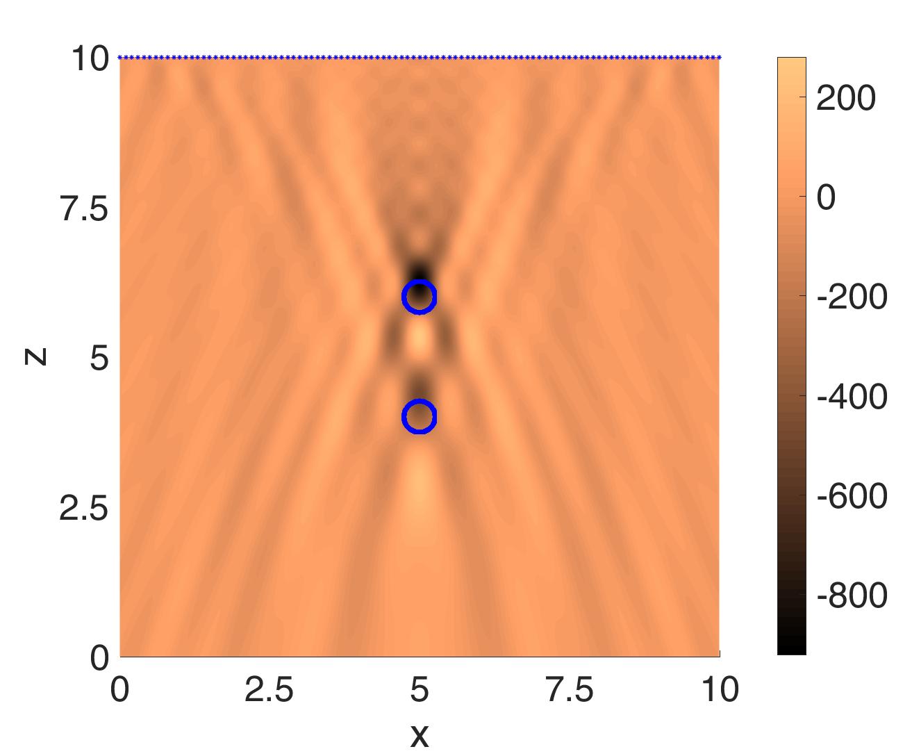
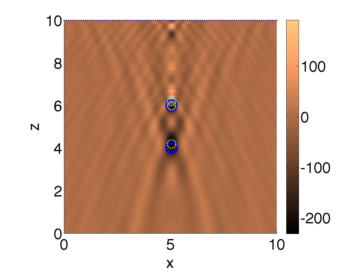
(c)                                                     (d)

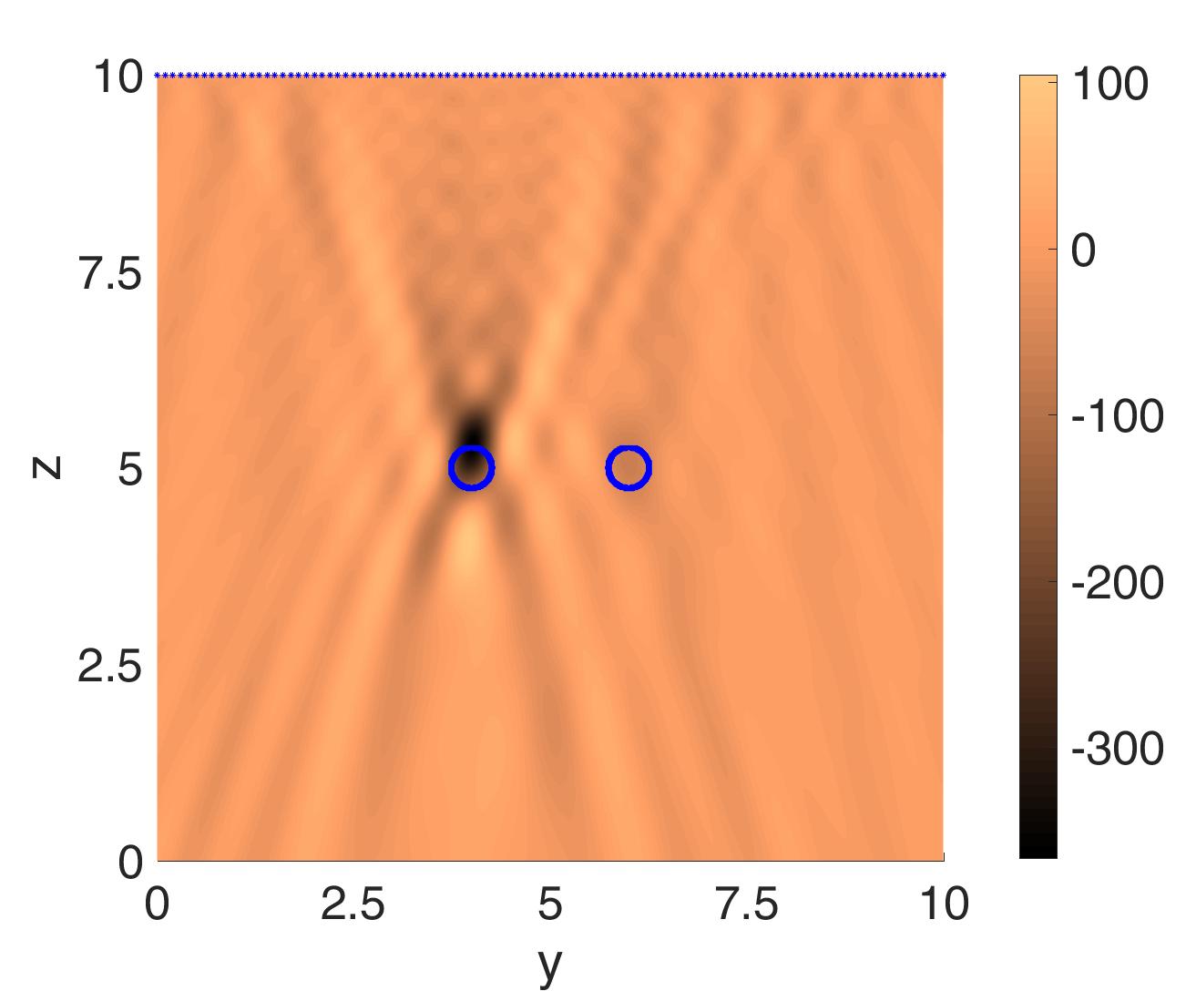
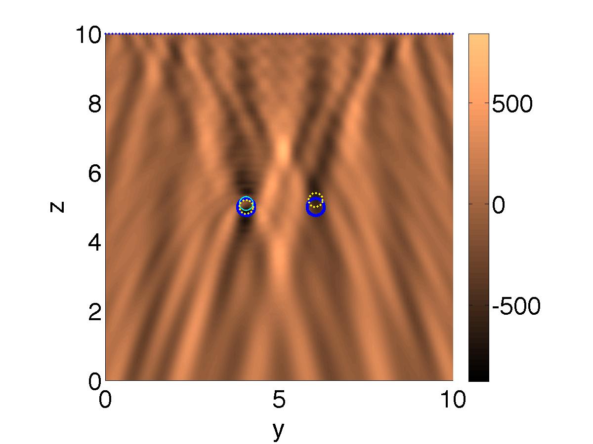
Figure 9: Iteration using topological derivatives of the holography cost functional (3) in geometries with multiple spheres. Two spheres along the $z$ axis with ${k}_{e}=12.6$ and ${k}_{i}=15.12$ in both spheres: (a) Slice $y=5$ of the topological derivative computed evaluating (8) with (11) and (15). Only the upper object is clearly distinguished. (b) Same as (a) but evaluating (19) with (4) and (25) when the approximate object is the sphere defined by the thin cyan contour and $k_{i}$ is taken as known. The lower object is now visible. Two spheres along the $y$ axis with ${k}_{e}=12.6$, ${k}_{i}=15.12$ in the leftmost sphere and ${k}_{i}=13.75$ in the rightmost sphere: (c) Slice $x=5$ of the topological derivative computed evaluating (8) with (11) and (15). Only the leftmost object is clearly distinguished. (d) Same as (c) but evaluating (19) with (4) and (25) when the approximate object is the sphere defined by the thin cyan contour and the approximate value of $k_{i}$ in it is $k_{i}^{(0)}=15.76$. The rightmost object is now visible.

Consider now two spheres along the $y$ axis. Figures 4(a)-(b) show that both are identified when $k_{i}$ takes similar values in them. Increasing the gap between the values of $k_{i}$, only the sphere corresponding to the largest value is detected initially, see the topological derivative in Figure 9(c). The topological energy has a similar aspect, and, as said before, does not use the value of $k_{i}$. We exploit it to initialize $\Omega^{(0)}$ by formula (17), recovering only the object with higher contrast.

Assuming the values of $k_{i}$ unknown, we next attempt to recover the number of objects and their parameters combining topological derivatives and descent techniques for the coefficients, as indicated in Fig. 10(a). We initialize ${k}_{i}$ as a perturbation ${k}_{i}^{(0)}$ of the ambient dimensionless wavenumber ${k}_{e}$, and iterate as follows. Given an approximation of the scatterers $\Omega^{(n)}$, we update the value of ${k}_{i}^{(n)}$ to obtain ${k}_{i}^{(n+1)}$ by a descent technique. The parameter to be optimized appears in the forward problem governing the electric field. A derivative of the cost functional with respect to it is given by (80). Choosing $k_{i}^{(n+1)}={k}_{i}^{(n)}+\delta\psi_{n}$, with $\delta>0$ small and

(27) $$\psi_{n}(\mathbf{x})=-{\rm Re}\left[E_{n}(\mathbf{x})\overline{P}_{n}(\mathbf{x})\right],\ \ \qquad{\mathbf{x}}\in\Omega^{(n)},$$

the functional decreases. $E_{n}$ and $P_{n}$ are forward and adjoint fields with object $\Omega^{(n)}$ and coefficient $k_{i}^{(n)}$ computed by BEM-FEM. If $\Omega^{(n)}=\bigcup_{\ell=1}^{L}\Omega_{\ell}^{(n)}$ and we are looking for piecewise constant parameters, we may take

(28) $$\psi_{n}(\mathbf{x})=-{1\over{\rm meas}(\Omega^{(n)}_{\ell})}{\rm Re}\int_{\Omega^{(n)}_{\ell}}E_{n}\overline{P}_{n},\ \ \qquad{\mathbf{x}}\in\Omega^{(n)}_{\ell},\;\ell=1,\ldots,L.$$

Setting $k_{i}^{(n,0)}=k_{i}^{(n)}$ we calculate:

(29) $${k}_{i}^{(n,m+1)}={k}_{i}^{(n,m)}+\delta\psi_{n,m}$$

with $\delta>0$ small enough to ensure $J({k}_{i}^{(n,m+1)})<J({k}_{i}^{(n,m)}).$ We have defined $\psi_{n,m}$ only in $\Omega^{(n)}.$ However, formulas (27) and (28) make sense everywhere, and (29) defines ${k}_{i}^{(n,m+1)}$ for ${\mathbf{x}}\in{\mathbb{R}}^{3}.$ After a number of iterations $M$, we stop, fix $k_{i}^{(n+1)}=k_{i}^{(n,M)}$ and update the approximation of the objects to obtain $\Omega^{(n+1)}$ by the scheme described in Fig. 8(a). From a computational point of view, updating $k_{i}^{(n)}$ is less expensive than updating $\Omega^{(n)}$ because the computational domain is fixed and already meshed. Therefore, it seems advisable at first sight to take $M>1$.

In view of (29), once the approximation $\Omega^{(0)}$ to the objects is proposed by (17), we initialize ${k}_{i}^{(0)}={k}_{e}+\delta\psi_{0}$ where $\psi_{0}$ is defined by (28), $E_{0}$ and $P_{0}$ being the forward and adjoint fields computed in the whole space by (11) and (14). Then formula (29) provides a new approximation $k_{i}^{(1)}$. We stopped the iteration at $M=10$ and computed $D_{T}(\mathbf{x},\Omega^{(0)},k_{i}^{(1)})$ by solving (4),(25) by BEM-FEM to produce $\Omega^{(1)}$ with (18). The location of the first object is corrected, and a new object is clearly seen, so that $\Omega^{(1)}$ is formed by two elongated components. The new component, however, is slightly displaced forward in the incidence direction. When we seek $k_{i}^{(2)}$ defined in both components we see that small variations in the previous process lead to very different results in the new one (corresponding to the object with lowest contrast).

(a)                                                (b)

Figure 10: Strategy to predict the permittivities of the objects for cost functional (79): (a) General procedure allowing for irregular domains and variable coefficients. (b) When we are interested in piecewise constant guesses or in studying the structure of the minima we may simplify the computational complexity by intermediate computations with spheres.

To understand this behavior, we revisit the approximation using the strategy in Fig. 10 (b). We fit a ball $\hat{\Omega}^{(0)}$ to $\Omega^{(0)}$ defined by (17), represented by the thin cyan contour in Figure 9(d). To produce a guess of $k_{i}$, we fix $\hat{\Omega}^{(0)}$ and evaluate the functional (3) for a range of $k_{i}$ using Appendix B. It reaches a minimum value at $k_{i}^{(0)}=15.76.$ Figure 9(d) depicts the topological derivative $D_{T}(\mathbf{x},{\mathbb{R}}^{3}\setminus\overline{\hat{\Omega}^{(0)}},k_{i}^{(0)}).$ The rightmost object is now clearly detected. The position of the leftmost one is corrected removing points from its top and adding them at the bottom, using (26) to generate a new guess $\Omega^{(1)}$, and then fitting spheres $\hat{\Omega}^{(1)}$ to it. We are left with two balls represented by the dotted yellow lines. To find a value for $k_{i}$ at the second sphere, we may fix the two spheres, use the known approximation of $k_{i}$ at the preexisting one, and minimize (3) with respect to the value of $k_{i}$ in the second one. However, we fail to find isolated local minima. A continuum exists. An isolated global minimum is only encountered when the offset in the location of the second object is reduced. Even if updating $k_{i}^{(n)}$ is less expensive than updating $\Omega^{(n)}$, as indicated before, for convergence reasons it may be advisable to choose $M=1$. However, this problem may disappear when the contrast with the ambient medium is more alike for the different objects.

5 Approximation of the electric field at the recording screen

The previous sections propose strategies to recover holographied objects from recorded in-line holograms ${\cal I}$ without a priori information. We have obtained initial guesses of objects, which can be improved by iteration to correct the number of components and their position. However, while the shapes in $xy$ planes are correct, they remain elongated in the $z$ direction. Ref. [7] showed in a similar setting and using the full electric field $E_{meas}$ as data that the elongation of the shape in the incidence direction could be removed by iteration. As said before, the electric field $E_{meas}$ cannot be measured in practice, instead we may develop mathematical methods to approximate it numerically from the hologram ${\cal I}$. We study here the possibility of approximating the full electric field $E_{meas}$ at the recording screen from the holograms ${\cal I}$ and then using this approximated field $E_{approx}$ to reconstruct the objects by topological methods.

5.1 Initial approximation of the electric field and the scatterers

Consider the imaging setting depicted in Fig. 1, with light of wavelength $660$ nm emitted at a distance of $10\,\mu$m from the recording screen. The incident wave $E_{inc}\sim 1$ at the detector screen. Setting $E_{inc}=1$ in the expansion

(30) $${\cal I}=|E_{meas}|=|E_{sc}+E_{inc}|^{2}=|E_{sc}|^{2}+|E_{inc}|^{2}+E_{sc}\overline{E_{inc}}+\overline{E_{sc}}E_{inc},$$

we may infer a rough approximation of the scattered field at the detectors. If we neglect the quadratic term $|E_{sc}|^{2}$, we find:

(31) $$E_{scapprox,j}^{(0)}=({\cal I}(\mathbf{x}_{j})-1)/2\sim{\rm Re}(E_{sc}),\quad j=1,\ldots,N.$$

Alternatively, we may set ${\rm Im}(E_{sc})=0$ and look for a solution of ${\rm Re}(E_{sc})^{2}+2{\rm Re}(E_{sc})+1-{\cal I}=0$ decaying to zero at the borders, which yields $E_{scapprox}^{(0)}={-1+\sqrt{\cal I}}.$ The true total electric field $E_{meas}$ at the detectors being unknown, we approximate it by

(32) $$E_{approx,j}^{(0)}=E_{scapprox,j}^{(0)}+E_{inc}(\mathbf{x}_{j}),\quad j=1,\ldots,N,$$

and consider the cost functional:

(33) $$J(\Omega)={1\over 2}\sum_{j=1}^{N}|E(\mathbf{x}_{j})-E_{approx,j}^{(0)}|^{2}.$$

The topological derivative and energy in $\mathbb{R}^{3}$ are given by (8) and (16), respectively, with forward field $E=E_{inc}$ and conjugate adjoint field [7]

(34) $$\overline{P}({\mathbf{x}})=-\sum_{j=1}^{N}{e^{\imath{k}_{e}|{\mathbf{x}}-{\mathbf{x}_{j}}|}\over 4\pi|{\mathbf{x}}-{\mathbf{x}_{j}}|}(\overline{E_{approx,j}^{(0)}-E(\mathbf{x}_{j})}).$$

We may use them to obtain initial guesses of the objects, as indicated in Fig. 11. The results are similar to the initial predictions of scatterers obtained in Section 3 using the holography cost functional (3), and in Ref. [7] using the cost functional (33) with the true synthetic data $E_{meas}$ instead of $E_{approx}$. This illustrates the fact that topological methods are very robust to noise. The $xy$ sections still suggest the true shape whereas the $xz$ sections locate the region occupied by the object, showing a certain elongation and shift towards the screen.

Figure 11: Procedure to recover objects using a crude approximation of the electric field at the detectors, obtained from the hologram using cost functional (33).

For light of wavelength $660$ nm we have approximated the electric field by at the detectors exploiting that $E_{inc}\sim 1$ at a screen located a distance $z_{0}=z_{i}+z_{p}=10$ from the light emitter. Similarly, for light of wavelength $405$ nm $E_{inc}\sim-\imath$ at the detectors. Then $\overline{E_{inc}}\sim\imath$ and $E_{sc}\overline{E_{inc}}+\overline{E_{sc}}E_{inc}\sim-2{\rm Im}(E_{sc})$. If we set $|E_{sc}|^{2}\sim 0$, we obtain:

(35) $$E_{scapprox}^{(0)}={\rm Im}(E_{sc})=(1-{\cal I})/2,$$

Alternatively, we may set ${\rm Re}(E_{sc})\sim 0$ and look for a solution of ${\rm Im}(E_{sc})^{2}-2{\rm Im}(E_{sc})+1-{\cal I}=0$ decaying to zero at the borders, which yields $E_{scapprox}^{(0)}={1-\sqrt{\cal I}}.$

A similar strategy may be used if $E_{inc}\sim-1$ or $E_{inc}\sim\imath$ at the screen, or for other values.

5.2 Improved approximation of the electric field

To be able to sharpen object guesses we need better approximations of the electric field. To obtain them, we use the hologram definition:

(36) $${\cal I}=|E_{sc}+E_{inc}|^{2}=|E_{inc}|^{2}+|E_{sc}|^{2}+E_{sc}\overline{E_{inc}}+\overline{E_{sc}}E_{inc},$$

which can be rewritten as

(37) $${\cal I}\!-\!|E_{inc}|^{2}={\rm Re}(E_{sc})^{2}\!+\!{\rm Im}(E_{sc})^{2}\!+\!2[{\rm Re}(E_{sc})\cos(k_{e}z_{0})\!+\!{\rm Im}(E_{sc})\sin(k_{e}z_{0})],$$

where $z_{0}$ is the distance from the emitter to the recording screen, or

(38) $${\cal I}-|E_{inc}|^{2}=r^{2}+r[e^{\imath\phi}e^{-\imath k_{e}z_{0}}+e^{-\imath\phi}e^{\imath k_{e}z_{0}}],\quad E_{sc}=re^{\imath\phi}.$$

At each fixed receptor, equations (37) and (38) are undetermined: one equation for two unknowns. Setting the real or imaginary parts equal to zero we obtain the crude approximations employed before. However, the true fields are solutions with non zero real and imaginary parts.

Our procedure to approximate the complex electric field at the detectors knowing the hologram is sketched in Figure 12. We define an error functional to quantify the difference between the true hologram and the hologram that would be observed using a prediction of the electric field at the receptors. Then, we combine a gradient method to reduce the error in our prediction of the electric field and a Gaussian filter to smooth out strong variations. To initialize the optimization procedure avoiding convergence to the already known solutions with zero real or imaginary part, we use the electric field scattered by spheres placed at the peaks of the topological energy fields computed using the explicit expressions in Appendix B. This procedure yields the approximations to the electric fields at the recording screen depicted in Figure 13. We detail the steps next.

Figure 12: Strategy to obtain a sharper approximation of the electric field at the detectors from the hologram, as well as a possibly better description of the geometry of the scatterers.

5.2.1 Gradient optimization

We define the following optimization problem: Find $E_{scapprox}\in\mathbb{C}^{N}$ minimizing

(39) $$F(E_{scapprox})=\sum_{j=1}^{N}|{\mathcal{I}}({\bf x}_{j})-|E_{scapprox,j}+E_{inc}({\bf x}_{j})|^{2}|^{2},$$

where ${\mathcal{I}}$ is the hologram recorded for the true scatterers.

Since the real and imaginary parts of our fields are strongly oscillatory, we use the polar representation of complex numbers and resort to a gradient technique. Let us set $E_{scapprox,j}=r_{j}e^{\imath\phi_{j}}$, ${\bf r}=(r_{1},\ldots,r_{N})$, ${\boldsymbol{\phi}}=(\phi_{1},\ldots,\phi_{N})$, and

(40) $$F({\bf r},{\boldsymbol{\phi}})=\sum_{j=1}^{N}|{\mathcal{I}}({\bf x}_{j})-|r_{j}e^{\imath\phi_{j}}+E_{inc}({\bf x}_{j})|^{2}|^{2}.$$

Then, the partial derivatives of the cost function are given by:

$${\partial F\over\partial r_{j}}=-4[{\mathcal{I}}({\bf x}_{j})-|r_{j}e^{\imath\phi_{j}}+E_{inc}({\bf x}_{j})|^{2}][(r_{j}e^{\imath\phi_{j}}+E_{inc}({\bf x}_{j}))e^{-\imath\phi_{j}}$$

(41) $$+(r_{j}e^{-\imath\phi_{j}}+\overline{E_{inc}({\bf x}_{j})})e^{\imath\phi_{j}}],$$

$${\partial F\over\partial\phi_{j}}=-4[{\mathcal{I}}({\bf x}_{j})-|r_{j}e^{\imath\phi_{j}}+E_{inc}({\bf x}_{j})|^{2}][-\imath(r_{j}e^{\imath\phi_{j}}+E_{inc}({\bf x}_{j}))r_{j}e^{-\imath\phi_{j}}$$

(42) $$+\imath(r_{j}e^{-\imath\phi_{j}}+\overline{E_{inc}({\bf x}_{j})})r_{j}e^{\imath\phi_{j}}].$$

We generate sequences along which the error functional decreases setting

$$(r_{1},\ldots,r_{N},\phi_{1},\ldots,\phi_{N})^{new}=(r_{1},\ldots,r_{N},\phi_{1},\ldots,\phi_{N})^{old}$$

(43) $$-\delta({\partial F\over\partial r_{1}},\ldots,{\partial F\over\partial r_{N}},{\partial F\over\partial\phi_{1}},\ldots,{\partial F\over\partial\phi_{N}})(r_{1},\ldots,r_{N},\phi_{1},\ldots,\phi_{N})^{old}.$$

The parameter $\delta>0$ might be chosen to take different values along different directions, though we will keep it uniform in our tests. We have set $\delta=0.1$.

To implement the gradient procedure we need to select an adequate initial value for the electric field. To do so, we exploit the information about the scatterers provided by the strategy sketched in Figure 11. We have two options:

• Use (17) to obtain a guess $\Omega^{(0)}$ of the scatterer geometry. The resulting shape for $\Omega^{(0)}$ is arbitrary. We then solve the forward problem (4) numerically to evaluate the corresponding scattered electric field $E_{scsynth}^{(0)}$ at the detectors. This can be done employing BEM-FEM as in [7].

• Fit balls $\Omega^{(0)}$ to the shapes predicted by (17). We then solve the forward problem (4) using series expansions in terms of spherical harmonics to evaluate the corresponding electric field $E_{scsynth}^{(0)}$ at the detectors, see Appendix B. This choice reduces the computational complexity.

The resulting scattered fields $E_{scsynth}^{(0)}$, however, do not satisfy (36). We use $E_{scsynth}^{0}$ as starting point to optimize (39). The scheme starts from $(r_{1},\ldots,r_{N},\phi_{1},\ldots,\phi_{N})^{0},$ obtained expressing $E_{scsynth,j}^{(0)}=r_{j}^{0}e^{\imath\phi_{j}^{0}}$, $j=1,\ldots,N$. Then, we update these values using identity (43), where the derivatives are given by formulas (41)-(42). The procedure stops when the cost functional (39) falls below a fixed threshold value.

Computing the electric field scattered by a sphere $E_{scsynth}^{(0)}$ requires the knowledge of the parameter ${k}_{i}$, that is, its permittivity. However, we only use this field as a starting value for the optimization procedure which avoids converging to purely real or imaginary solutions. We have checked that the output of the gradient scheme is not really sensitive to variations of ${k}_{i}$ in a wide range of values. In case ${k}_{i}$ was unknown, setting it equal to a small perturbation of ${k}_{e}$ would produce a reasonable approximation of the electric field at the detectors.

5.2.2 Gaussian filter

The corrections provided by the gradient procedure described in Section 5.2.1 are local, in the sense that the evolution at one detector is not influenced by the evolution at the neighboring ones. Since the fields are oscillatory, this may result in spurious local spikes. Large errors at some points will compensate very small errors at other points. To overcome this problem we successively distribute the error using a Gaussian filter [12, 24].

Given a Gaussian $G(x,y)=Ae^{\frac{-((x-x_{0})^{2}+(y-y_{0})^{2})}{2\sigma^{2}}}$ centered at $(x_{0},y_{0})$ and a function $E_{scapprox}(x,y)$, we define the discrete convolution as

(44) $$\hskip 17.07164ptE_{scfilter}(x,y)=E_{scapprox}*G(x,y)=\sum_{i=-\infty}^{\infty}\sum_{j=-\infty}^{\infty}G(i,j)E_{scapprox}(x-i,y-j).$$

For numerical purposes we select a finite approximation, in the form of a $3\times 3$ matrix:

$$G(i,j)=Ae^{-\frac{(i-2)^{2}+(j-2)^{2}}{2\sigma^{2}}},\quad A^{-1}=\sum_{i=1}^{3}\sum_{j=1}^{3}e^{-\frac{(i-2)^{2}+(j-2)^{2}}{2\sigma^{2}}}.$$

The filtered field is:

(45) $$E_{scfilter}(i,j)=\sum_{k=1}^{3}\sum_{l=1}^{3}G(k,l)E_{scapprox}(i-2+k,j-2+l),$$

$$G=\left(\begin{matrix}0.0113&0.0838&0.0113\\ 0.0838&0.6193&0.0838\\ 0.0113&0.0838&0.0113\\ \end{matrix}\right).$$

This function is smoother than the original one and can be used as starting point for a new gradient procedure. Better results might be obtained using adaptive filters, which vary in space.

(a)                   (b)                   (c)                   (d)

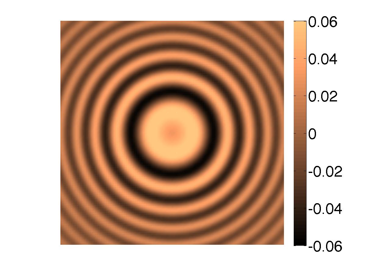
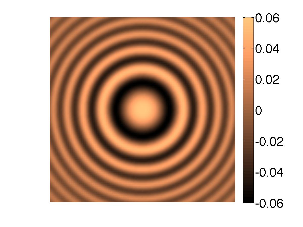
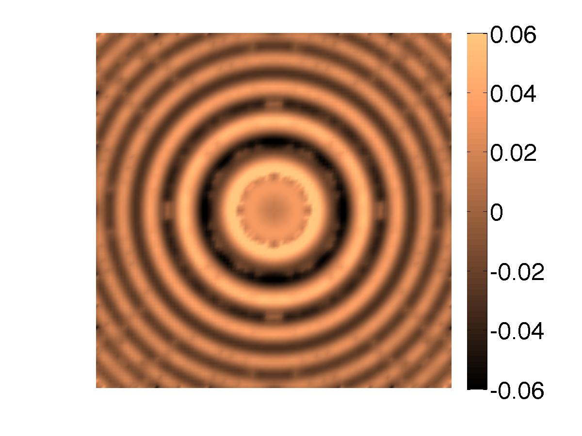
(e)                   (f)                   (g)                   (h)

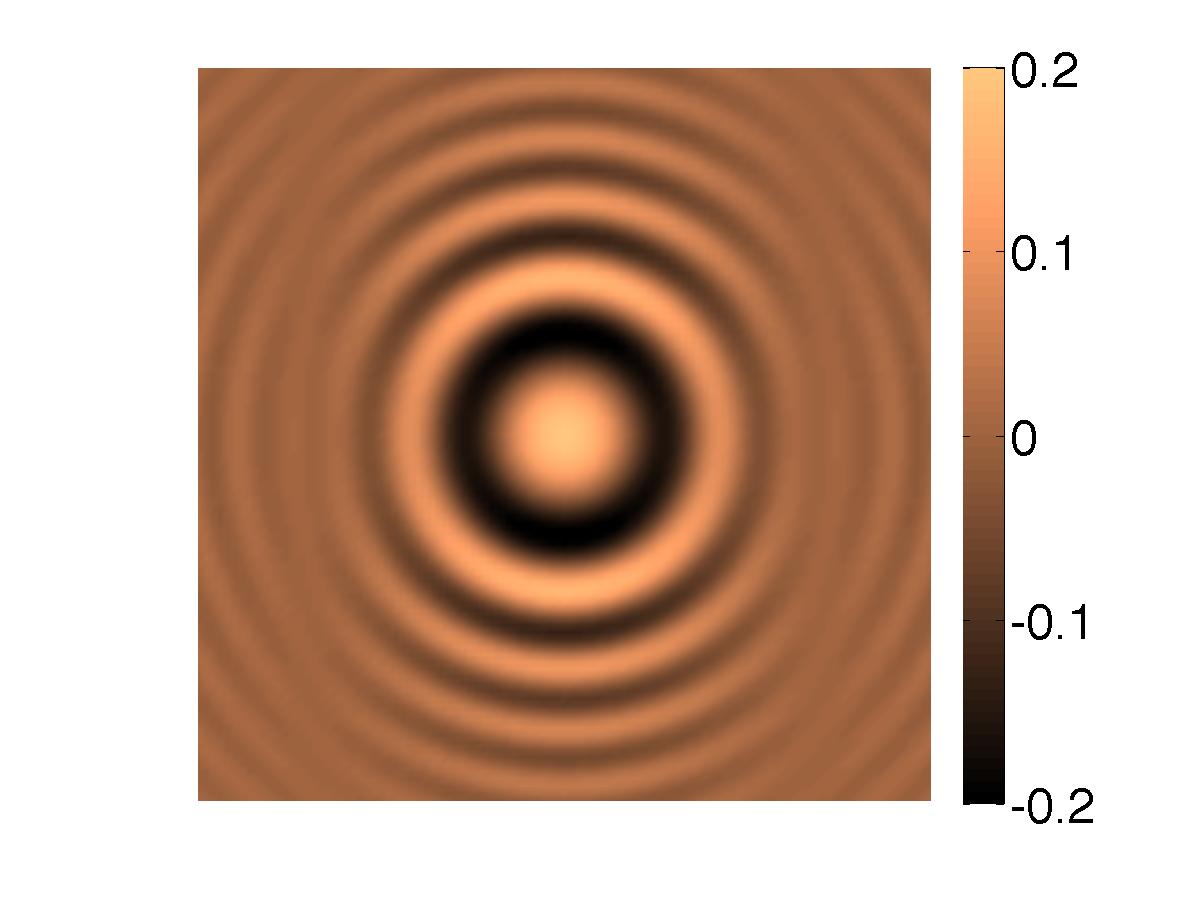
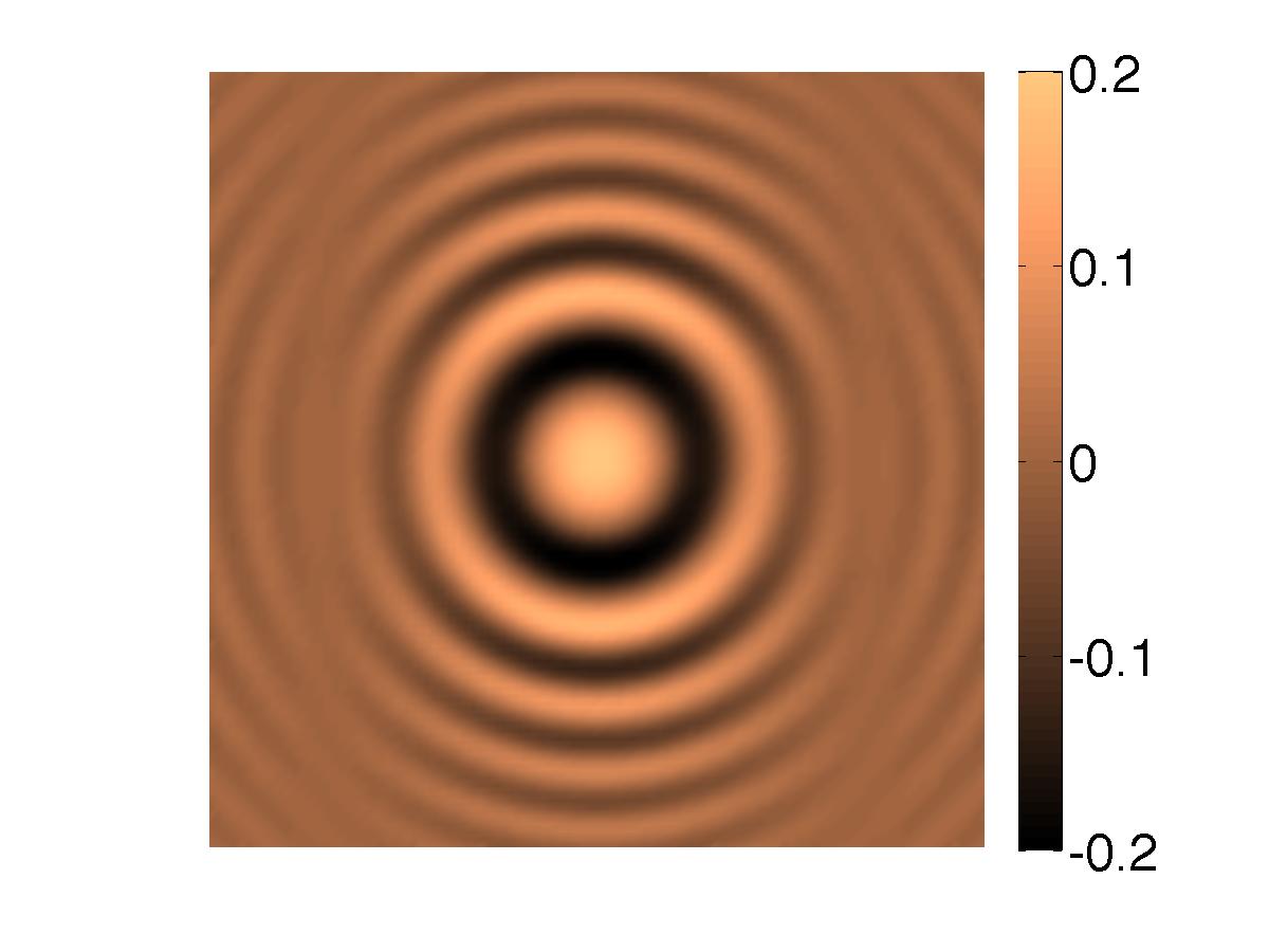
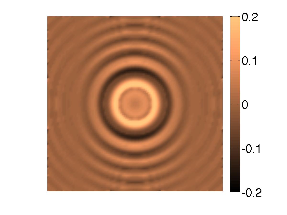
(i)                   (j)                   (k)                   (l)

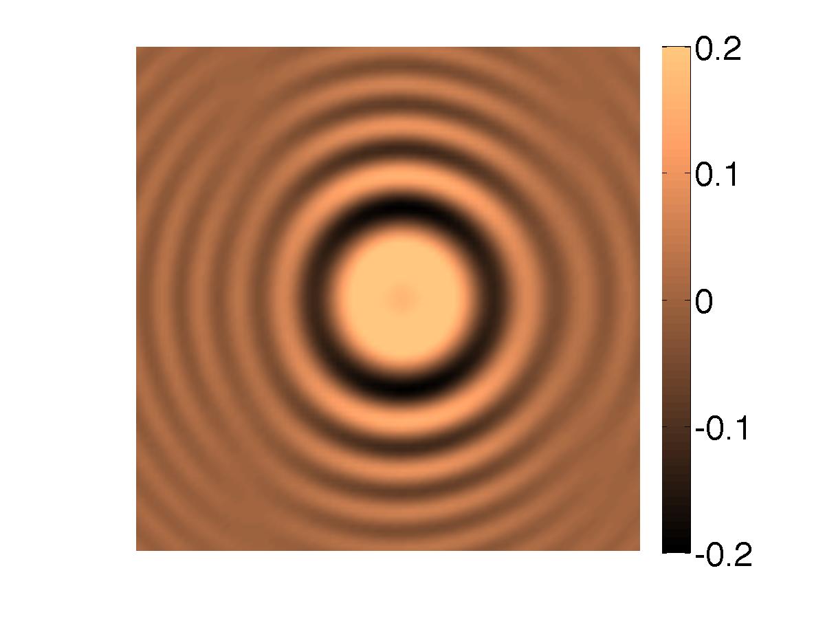
(m)                   (n)                   (o)                   (p)

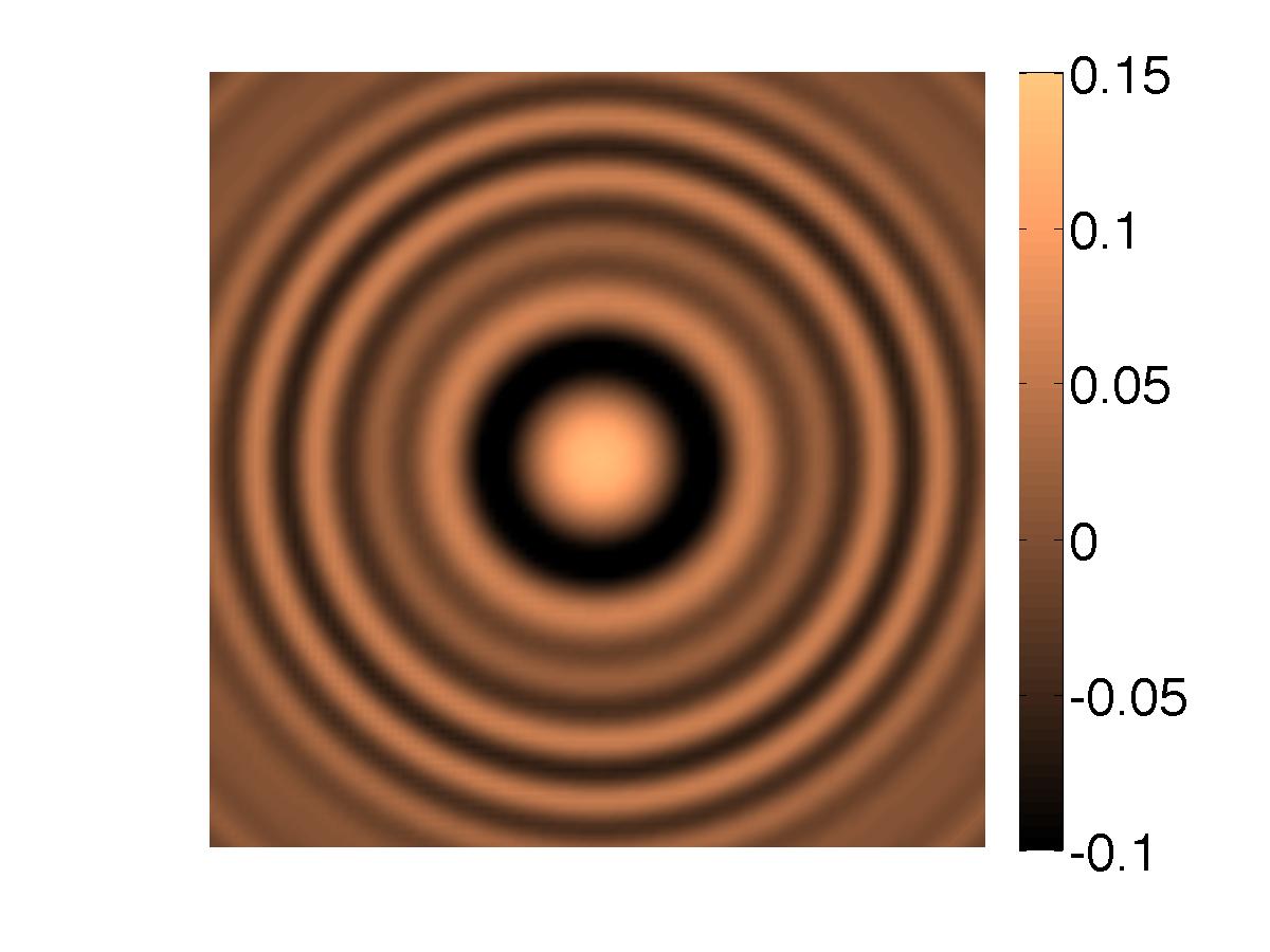
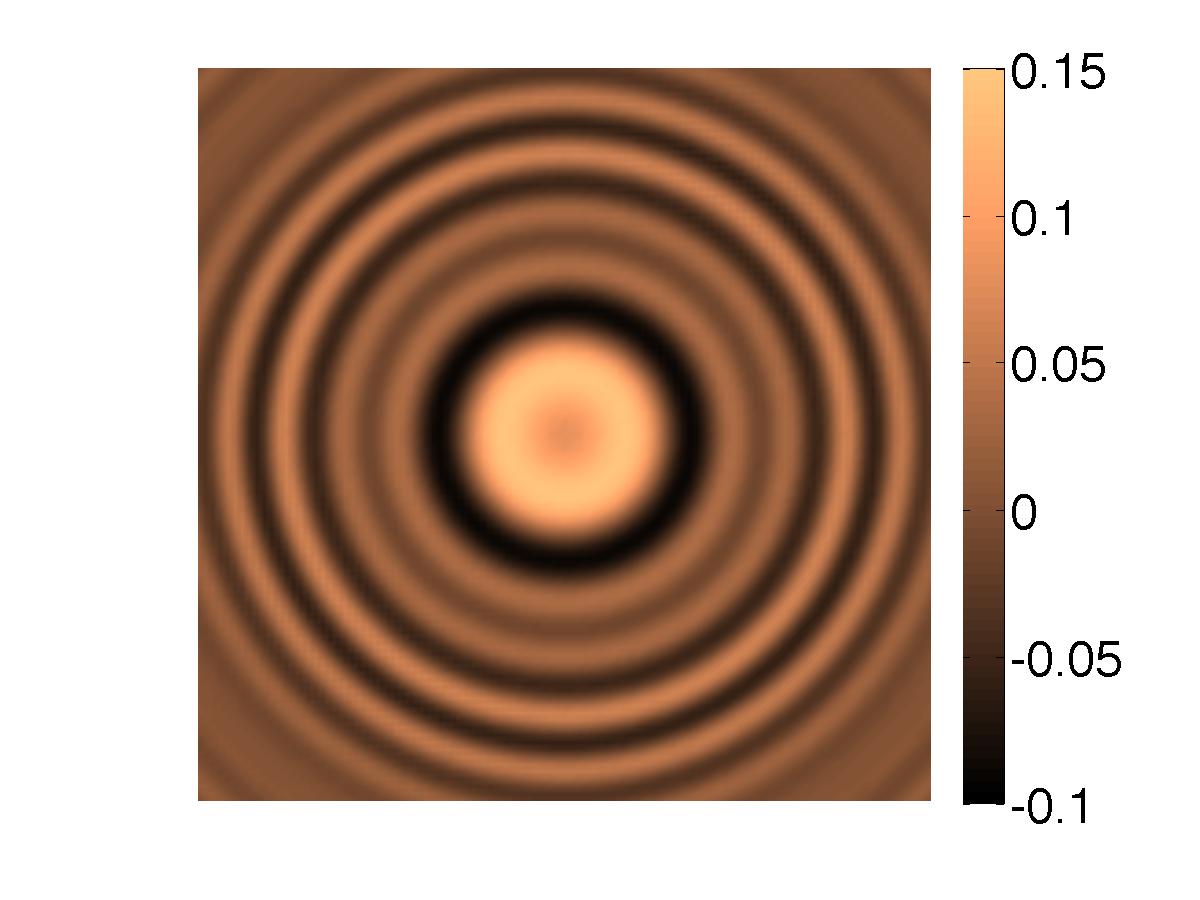
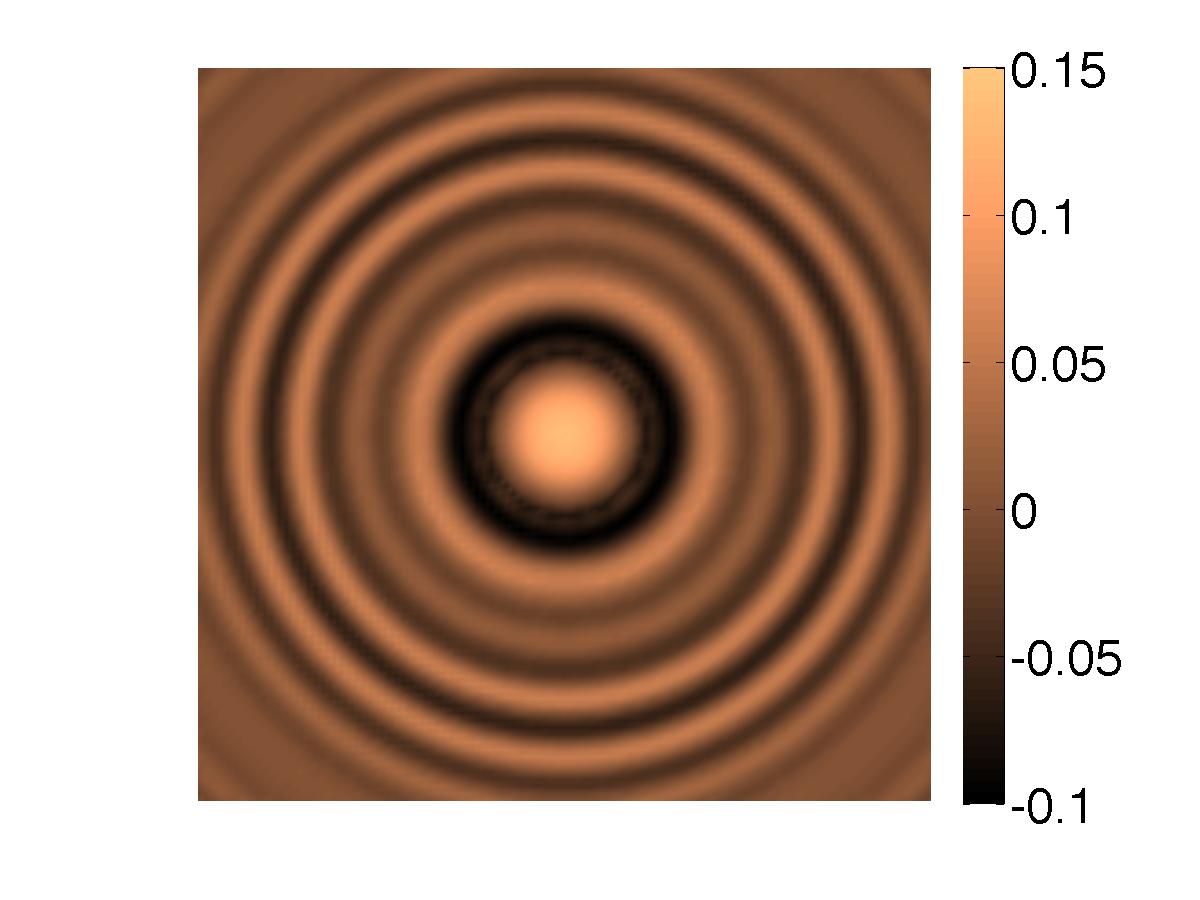
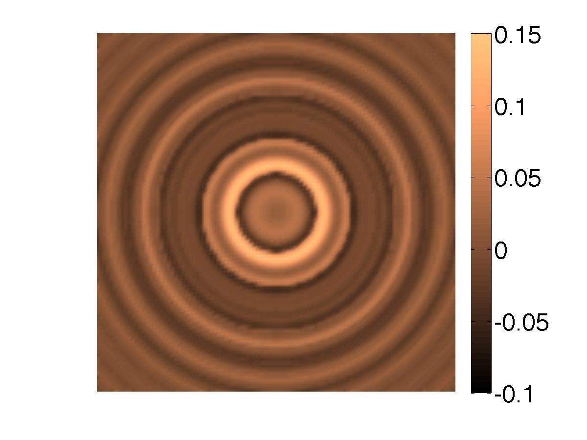
(q)                   (r)                   (s)                   (t)

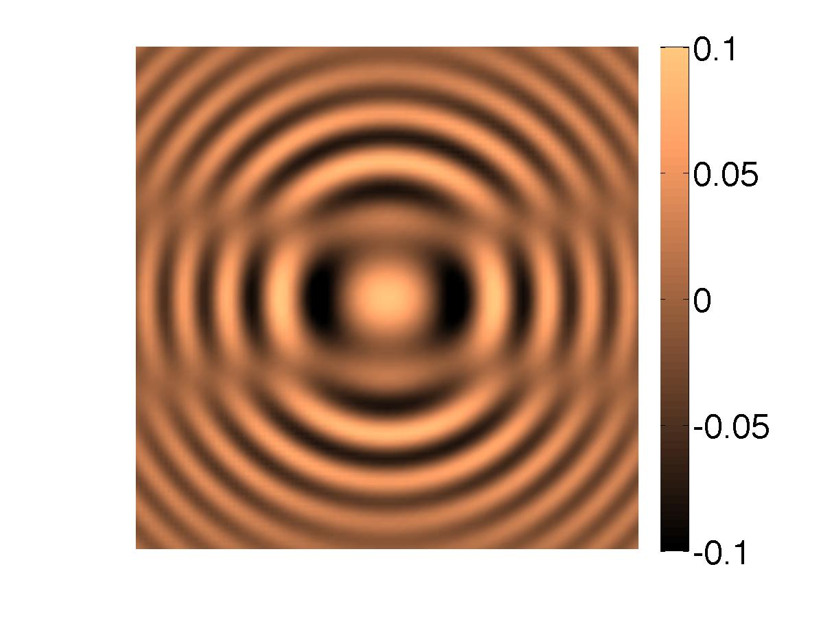
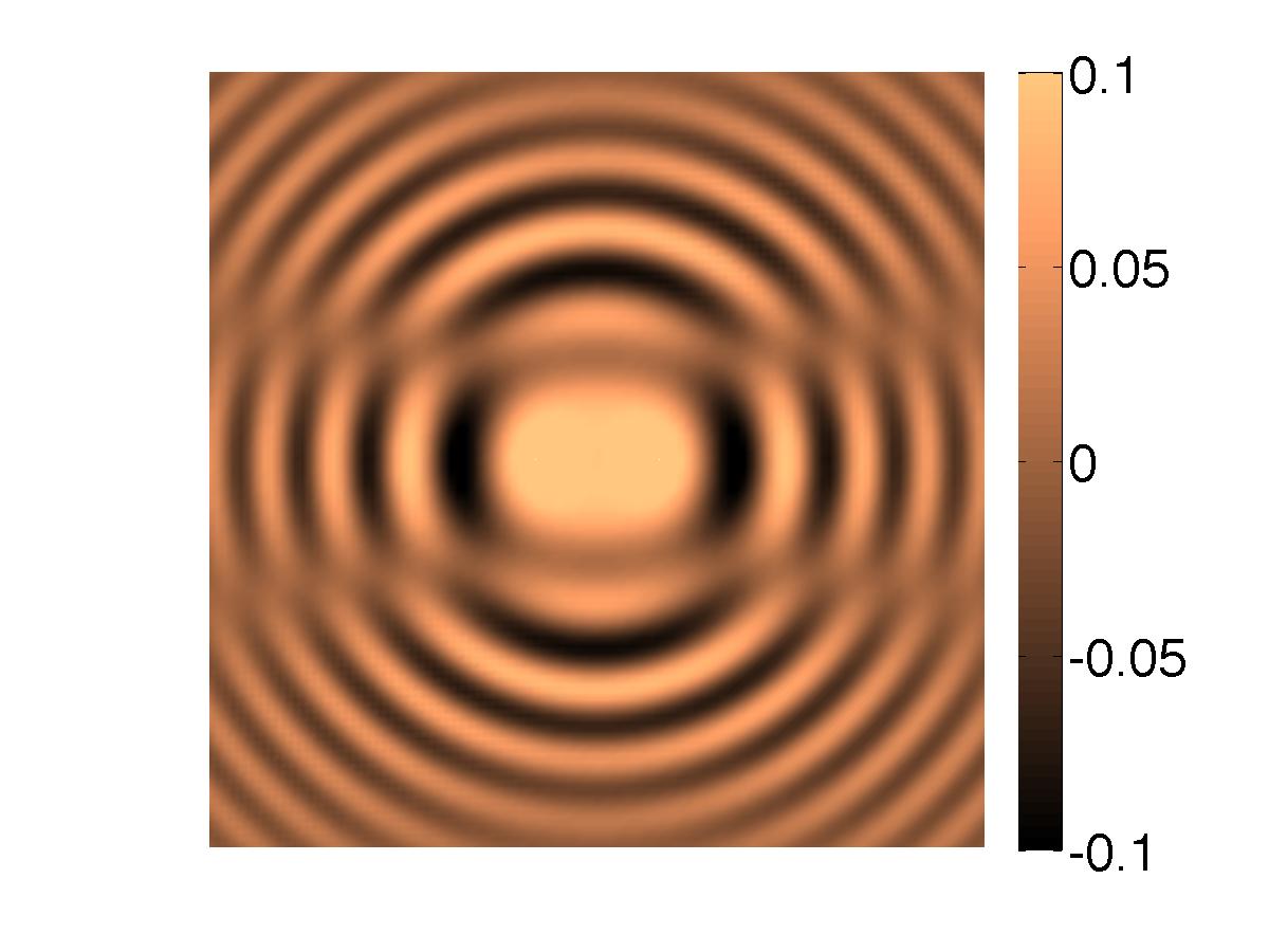
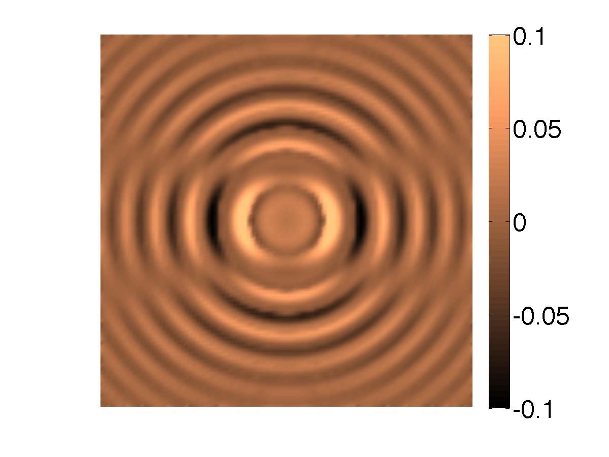
     $Re(E_{sc})$            $Im(E_{sc})$           $Re(E_{scapprox}^{(1)})$      $Im(E_{scapprox}^{(1)})$

Figure 13: True versus approximated real and imaginary parts of the scattered electric fields for objects with ${k}_{i}=15.12$ in a medium with ${k}_{e}=12.6$. (a)-(d) Sphere of diameter $0.5$ ($500$ nm). (e)-(h) Spherocylinder of diameter $0.5$ and length $1$ along the $x$ axis. (i)-(l) Pear-like object of maximum diameter $0.5$ along the $x$ axis. (m)-(p) Two spheres of diameter $0.5$ along the $z$ axis. (q)-(t) Two spheres of diameter $0.5$ along the $y$ axis.

5.2.3 Combined gradient and filter corrections

We will resort to an optimization strategy combining gradient variations and Gaussian filtering, see Figure 12:

• $E_{scsynth}^{(0)}$ is the initial approximation obtained from $E_{scapprox}^{(0)}$.

• $E_{scgradient}^{(1)}$ is the outcome of applying the gradient procedure (43) starting from $E_{scsynth}^{(0)}$.

• At each stage $n$

  • $E_{scfilter}^{(n)}$ is the outcome of convolving $E_{scgradient}^{(n)}$ with the Gaussian filter (45).

  • $E_{scgradient}^{(n+1)}$ is the outcome of applying the gradient procedure (43) starting from $E_{scfilter}^{(n)}$.

The final result is the new approximation of the scattered electric field $E_{scapprox}^{(1)}$. Then, the approximation of the total measured field $E_{meas}$ would be:

(46) $$E_{approx}^{(1)}=E_{scapprox}^{(1)}+E_{inc},$$

which can be used to obtain better approximations of the objects by topological methods replacing $E_{approx}^{(0)}$ in functional (33).

5.2.4 Numerical results

Figure 13 compares the scattered electric fields of different objects recorded at the detectors with the approximation $E_{scapprox}^{(1)}$ produced by the above algorithm, summarized in Figure 12. The true electric fields are computed synthetically, solving the forward problem (4) for the chosen object by BEM-FEM. For the isolated sphere, we have combined $16$ steps, stopping in each of them the gradient algorithm when the cost functional became smaller than $10^{-9}$. We define the $\ell^{2}$ error when comparing two functions $f$ and $g$ as $\left(\sum_{j=1}^{N}|f({\mathbf{x}}_{j})-g({\mathbf{x}}_{j})|^{2}\right)^{1/2}.$ The $\ell^{2}$ error between the true and approximated electric field for a single ball falls below $10^{-1}$. For the remaining shapes, this is the case for the real parts. The imaginary parts show a reasonable qualitative agreement. However, the quantitative relative error in the central part is of order one. Alternating one or two gradient iterations with one Gaussian convolution during $16$ steps provides better and faster results than waiting until the cost functional is very small at each step unless we deal with single spheres. In our tests, the worst approximation of the imaginary part corresponds to a geometry of two spheres aligned along the $z$ axis, see Figure 13(p). Notice that only one sphere has been used to produce this approximation of the electric field, fitted to the most prominent bright area in Figure 4(d). It improves once we detect the second component of the object by the procedure in Fig. 12 and use it to generate a new prediction $E_{scapprox}^{(2)}.$

The fields depicted in Figure 13 have been computed using the known value of ${k}_{i}$ to evaluate $E_{scsynth}^{(0)}$ and then $E_{scapprox}^{(1)}.$ In biological and soft matter applications ${k}_{i}$ is usually slightly larger than ${k}_{e}$. We have checked that $E_{scapprox}^{(1)}$ does not change significantly varying ${k}_{i}$ in an interval $[{k}_{e}+0.5,{k}_{e}+6]$. This fact suggests that we would be able to approximate the electric field at the detectors even if ${k}_{i}$ was unknown.

We have exploited the predicted electric fields $E_{approx}^{(1)}$ to produce first guesses of the scatterers following the procedure sketched in Figure 12 with cost functionals of the form (33). The results are similar to those in Figures 2-4, 7 and 9. When we seek to sharpen the approximation of general shapes in the $z$ direction by iteration following the scheme in Fig. 8(a), the subsequent domains still keep some elongation in the $z$ direction. The performance of the method in this respect seems to be limited by the quality of the approximation of the electric field. Since the use of the true synthetic electric fields as data may remove the elongation [7], improved predictions of the objects would be expected by succesfully improving the numerical approximation of the electric field. Considering the shapes studied in Section 4, the predictions of unknown $k_{i}$ are comparable, except that now $k_{i}$ tends to be underestimated, not overestimated. The corrections of the shapes follow similar trends.

6 Conclusions

We have adapted topological field based imaging to work with the experimentally measurable holographic intensity. Assuming pure polarization of the incident light and neglecting the non polarized components of the electric field, we can reconstruct objects recorded in an in-line hologram with only the wavelength of the single incident wave and the ambient permittivity as prior information. The method we present here works in the scalar field approximation. This should be valid for many experiments, but future work can extend the method to the full vector Maxwell equations.

By tracking peaks of the topological fields, we can detect multiple objects, convex and non convex shapes, ranging from sizes comparable to the employed wavelength to sizes of a few nanometers, with nanometer precision. Our method does not require any specific object parametrization. Initial reconstructions show a different resolution in the incidence direction of the light and on planes orthogonal to it. Whereas shapes, sizes and positions are reasonably approximated on $xy$ planes, objects are displaced and elongated in the direction $z$. This later feature undergoes a transition as the size of the object grows above the wavelength, which facilitates its location in the $z$ direction between peaks of the topological fields. Here, we consider sizes below this transition. We show that the information on the number of objects and their positions provided by the initial reconstructions may be corrected by iteration. To this purpose, we propose strategies based on two different functionals. The first one quantifies the deviation between the hologram created by the true object and the hologram associated to the proposed shape, generated numerically. The second one replaces the hologram by an approximation of the full electric wave field obtained numerically from it. In both cases, their topological derivatives and topological energies produce similar initial reconstructions, which illustrates the robustness of these methods to noise. Then, topological derivative based iterations allow us to remove the offset and detect scatterers that might have be missed in the initial reconstruction, as a result of the presence of more prominent ones (due to their location or to higher permittivity contrast). Moreover, when the optical properties of objects are unknown, they can be inferred in an additional optimization step. The results obtained with the first functional are more straightforward. However, the second functional might have the potential to allow for better results, since reconstructions using synthetic electric fields as data have been shown to have the ability to the remove the elongation [7] by iteration. Currently, this possibility is limited by the quality of our numerical predictions of the electric field, obtained here by a combination of topological methods, gradient techniques and gaussian filters. Notice that the light field scattered by objects $E_{sc}$ is not a measurable magnitude in practice. Only interference patterns such as holograms $|E_{sc}+E_{inc}|^{2}$ are measurable. We succeed in obtaining reasonable numerical predictions of the electric field at the detectors though. This might pave the way to adapt to this framework techniques developed for larger wavelengths based on the knowledge of the full electric field at the detectors [3, 8, 9, 18, 30, 37, 49, 51].

We have focused here on methods that need no a priori information, but may use it if available, as shown in Figure 9. This technique could serve to determine priors for bayesian methods [14, 18]. Complementary shape or parameter optimization techniques might be incorporated to refine the approximation as well [10, 16, 38], using this holography functional and adjoint. In case the exact number of objects is determined, shape optimization based on deforming contours may improve the descriptions of shapes [10]. When a good approximation to permittivity variations is available, Newton type algorithms [8, 9, 37, 49, 51] may be used to refine it. Restrictions in the incidence directions and the extent of the recording region increase the possibility of converging to spurious minima in the optimization reformulations of the inverse problems unless good enough initial guesses of objects and permittivities are encountered. This type of inverse problems being ill posed, the quality of the final reconstruction is limited by the choice of incident directions (only one in these microscopy set-ups), the spread of the region where data are recorded (a flat screen behind the objects) and the distance to it.

Appendix A Derivatives of the holography cost functional

As a previous step to differentiate functional (3), we rewrite the constraint (4) in variational form. First, we replace the transmission problem (4) by an equivalent problem set in a bounded region $B_{R}$ containing the objects $\Omega$ and the detectors $\mathbf{x}_{j}$, $j=1,\ldots,N$. To do so, we take $B_{R}$ to be a ball of large enough radius $R$ with boundary $\Gamma_{R}=\partial B_{R}$. The Dirichlet–to–Neumann (also called Steklov–Poincaré) operator associates to any Dirichlet data on $\Gamma_{R}$ the normal derivative of the solution of the exterior Dirichlet problem:

$$\begin{array}[]{rcl}L_{k_{e}}:H^{1/2}(\Gamma_{R})&\longrightarrow&H^{-1/2}(\Gamma_{R})\\ f&\longmapsto&\partial_{\bf n}w\end{array}$$

where $w\in H^{1}_{loc}(\mathbb{R}^{3}\setminus\overline{B}_{R}),$ is the unique solution of

$$\left\{\begin{array}[]{ll}\Delta w+k_{e}^{2}w=0,&\qquad\mbox{in $\mathbb{R}^{3}\setminus\overline{B}_{R}$},\\ w=f,&\qquad\mbox{on $\Gamma_{R}$},\\ \displaystyle\lim_{r\to\infty}r(\partial_{r}w-\imath k_{e}w)=0.\end{array}\right.$$

$H^{1}_{loc}(\mathbb{R}^{3}\setminus\overline{B}_{R})$ denotes the Sobolev space of functions that are locally in $H^{1}$, whereas $H^{1/2}(\Gamma_{R})$ and $H^{-1/2}(\Gamma_{R})$ are the trace spaces [23, 42]. The vector $\mathbf{n}$ is the unit outer normal. This operator allows us to replace the radiation condition at infinity by a non–reflecting boundary condition on $\Gamma_{R}$ [29]: $\partial_{\bf n}(E-E_{inc})=L_{k_{e}}(E-E_{inc}).$ The variational formulation of problem (4) becomes: Find $E\in H^{1}(B_{R})$ such that

(47) $$b(\Omega;E,v)=\ell(v),\qquad\forall v\in H^{1}(B_{R}),$$

$$\begin{array}[]{rcl}{\rm with\hskip 39.83368pt}\displaystyle b(\Omega;E,v)&:=&\displaystyle\int_{B_{R}\setminus\overline{\Omega}}(\nabla E\nabla{\overline{v}}-k_{e}^{2}E{\overline{v}})d{\bf z}+\int_{\Omega}(\beta\nabla E\nabla{\overline{v}}-\beta k_{i}^{2}E{\overline{v}})d{\bf z}\\ &&\displaystyle-\int_{\Gamma_{R}}L_{k_{e}}(E)\,\overline{v}\,dS,\qquad\forall E,\,v\in H^{1}(B_{R}),\\ \ell(v)&:=&\displaystyle\int_{\Gamma_{R}}(\partial_{\bf n}E_{inc}-L_{k_{e}}(E_{inc}))\,\overline{v}\,dS,\qquad\forall v\in H^{1}(B_{R}).\end{array}$$

Assuming that $k_{e}$ is constant near $\Gamma_{R}$ and outside $B_{R}$, existence of a unique solution is guaranteed for bounded $k_{e}(\mathbf{x})$ and $k_{i}(\mathbf{x})$, and Lipschitz domains $\Omega$ [35, 42, 41]. Elliptic regularity for $-\Delta$ implies then that the solution belongs to $H^{2}(\Omega^{\prime})$ for any smooth $\Omega^{\prime}\subset\Omega$ or $\Omega^{\prime}\subset B_{R}\setminus\overline{\Omega}$ [23, 25]. Sobolev’s embeddings ensure continuity in $\Omega^{\prime}$, and continuity of derivatives when $k_{e}$,$k_{i}$ are differentiable ($W^{1,\infty}$ suffices) and bounded. When $\Omega$ is a $C^{2}$ domain [23], we may take $\Omega^{\prime}=\Omega,B_{R}\setminus\overline{\Omega}$, and, in fact, the solution is continuous in $\mathbb{R}^{3}$. If $k_{e}$ and $k_{i}$ are constant, the solution admits integral expressions both in $\Omega$ and $\mathbb{R}^{3}\setminus\overline{\Omega}$ in terms of the Green functions of Helmholtz equations [11, 35, 42]. In absence of $\Omega$, $E$ is as smooth as $E_{inc}$ permits.

A.1 Topological derivative

Given a region ${\cal R}\subset\mathbb{R}^{3}$, the topological derivative is a scalar field defined for each $\mathbf{x}\in{\cal R}$, which measures the variation of the functional when removing from ${\cal R}$ small balls $B_{\varepsilon}=B({\mathbf{x}},\varepsilon)$ centered at $\mathbf{x}$ [46]:

(48) $$\hskip 11.38109ptD_{T}({\mathbf{x}},{\cal R}):=\lim_{\varepsilon\to 0}{J({\cal R}_{\varepsilon})-J({\cal R})\over{\cal V}(\varepsilon)},$$

where ${\cal V}(\varepsilon)={4\over 3}\pi\varepsilon^{3}$ is the volume of a three dimensional ball of radius $\varepsilon$.

Theorem 1. When $k_{e}$, $k_{i}$, and $\beta$ are constant the topological derivative of functional (3) with $\Omega=\emptyset$ is given by

(49) $$\hskip 8.53581ptD_{T}(\mathbf{x},\mathbb{R}^{3})={\rm Re}\left[3{1-\beta\over 2+\beta}\nabla E(\mathbf{x})\!\cdot\!\nabla\overline{P}(\mathbf{x})\!+\!(\beta k_{i}^{2}-k_{e}^{2})E(\mathbf{x})\overline{P}(\mathbf{x})\right],\;\mathbf{x}\in\mathbb{R}^{3},$$

where $E$ is the solution of the forward problem:

(52) $$\left\{\begin{array}[]{ll}\Delta E+{k}_{e}^{2}E=0&\quad\mbox{in ${\mathbb{R}}^{3}$},\\ \displaystyle\lim_{r\to\infty}r\big{(}\partial_{r}(E-E_{inc})-\imath{k}_{e}(E-E_{inc})\big{)}=0,\end{array}\right.$$

and $\overline{P}$ is the solution of the conjugate adjoint problem:

(55) $$\left\{\begin{array}[]{ll}\Delta\overline{P}+{k}_{e}^{2}\overline{P}=2\sum_{j=1}^{N}({\mathcal{I}}-|E|^{2})\overline{E}\,\delta_{{\mathbf{x}}_{j}}&\quad\mbox{in ${\mathbb{R}}^{3}$},\\ \displaystyle\lim_{r\to\infty}r\big{(}\partial_{r}\overline{P}-\imath{k}_{e}\overline{P}\big{)}=0,\end{array}\right.$$

$\delta_{\mathbf{x}_{j}}$ being Dirac masses supported at the receptors. For a plane wave, $E=E_{inc}$ and $\overline{P}$ is given by:

(56) $$\overline{P}({\mathbf{x}})=-\sum_{j=1}^{N}{e^{\imath{k}_{e}|{\mathbf{x}}-{\mathbf{x}_{j}}|}\over 4\pi|{\mathbf{x}}-{\mathbf{x}_{j}}|}[2({\mathcal{I}}({\mathbf{x}_{j}})-|E({\mathbf{x}_{j}})|^{2})\overline{E}(\mathbf{x}_{j})].$$

Proof. To prove this expression, we set ${\cal R}=\mathbb{R}^{3}$ and exploit the relation with shape derivatives established in [20] :

(57) $$\hskip 11.38109ptD_{T}({\mathbf{x}},{\cal R})=\lim_{\varepsilon\to 0}\frac{<D{J}({\cal R}_{\varepsilon}),\mathbf{V}>}{{\cal V}^{\prime}(\varepsilon)}=\lim_{\varepsilon\to 0}\frac{1}{{\cal V}^{\prime}(\varepsilon)}\,\frac{d}{d\tau}{J}(\varphi_{\tau}({\cal R}_{\varepsilon}))\Big{|}_{\tau=0},$$

where ${\cal V}^{\prime}(\varepsilon)=4\pi\varepsilon^{2}$ and ${\cal R}_{\varepsilon}={\cal R}\setminus\overline{B_{\varepsilon}}$. The vector field $\mathbf{V}$ is an extension to $\mathbb{R}^{3}$ of $\mathbf{V}=-\mathbf{n}({\mathbf{z}}),\,{\mathbf{z}}\in\Gamma_{\varepsilon}=\partial B_{\varepsilon}({\mathbf{x}}),$ where the normal $\mathbf{n}(\mathbf{z}):={\mathbf{x}-\mathbf{z}\over|\mathbf{x}-\mathbf{z}|}$ points inside the ball, and vanishes away from a narrow neighborhood of $\partial B_{\varepsilon}$. The shape derivative along the vector field ${\bf V}$ is defined as

(58) $$<D{J}({\cal R}_{\varepsilon}),\mathbf{V}>:=\frac{d}{d\tau}\,{J}(\varphi_{\tau}({\cal R}_{\varepsilon}))\Big{|}_{\tau=0},$$

for the family of deformations $\varphi_{\tau}({\mathbf{z}}):={\mathbf{z}}+\tau{\bf V}({\mathbf{z}}),\,{\mathbf{z}}\in\mathbb{R}^{3},$ $\tau>0$. For any region ${\cal R}$, the deformed domain $\varphi_{\tau}({\cal R})$ is the image of ${\cal R}$ by the deformation: $\varphi_{\tau}({\cal R})=\{\mathbf{z}+\tau\mathbf{V}(\mathbf{z})\;|\;\mathbf{z}\in{\cal R}\}.$ Evaluating ${J}$ on the deformed regions, we define a scalar function ${J}(\varphi_{\tau}({\cal R}))$ of the deformation parameter $\tau$ which can be differentiated with respect to it.

Step 1: Computation of the shape derivative. We evaluate (3) in the deformed domains ${\cal R}_{\varepsilon,\tau}=\varphi_{\tau}({\cal R}_{\varepsilon})$, and denote by $E_{\varepsilon,\tau}\in H^{1}(B_{R})$ the solution of (47) with object $B_{\varepsilon,\tau}$. Notice that $\mathbf{V}$ vanishes on $\Gamma_{R}$, and at $\mathbf{x}_{j}$, $j=1,\ldots,N$. Differentiating with respect to $\tau$ we obtain

(59) $$\frac{d}{d\tau}\,J({\cal R}_{\varepsilon,\tau})\bigg{|}_{\tau=0}=2\,{\rm Re}\bigg{[}\sum_{j=1}^{N}(|E_{\varepsilon}(\mathbf{x}_{j})|^{2}-{\cal I}(\mathbf{x}_{j}))\overline{E_{\varepsilon}(\mathbf{x}_{j})}\dot{E}_{\varepsilon}(\mathbf{x}_{j})\bigg{]},$$

where $E_{\varepsilon}=E_{\varepsilon,0}$ and $\dot{E}_{\varepsilon}=\frac{d}{d\tau}\,E_{\varepsilon,\tau}\big{|}_{\tau=0}$. We follow [19, 20] and evaluate this derivative avoiding the computation of $\dot{E}_{\varepsilon}$ by introducing the Lagrangian functional

$${\cal L}({\cal R}_{\varepsilon,\tau};v,p):=J({\cal R}_{\varepsilon,\tau})-\mbox{Re}[b(B_{\varepsilon,\tau};v,p)-\ell(p)],\qquad\forall v,\,p\in H^{1}(B_{R}).$$

Using ${\cal L}({\cal R}_{\varepsilon,\tau};E_{\varepsilon,\tau},p)=J({\cal R}_{\varepsilon,\tau})$, (58) and (59) we obtain for any $p\in H^{1}(B_{R})$

(60) $$<DJ({\cal R}_{\varepsilon}),\mathbf{V}> = \frac{d}{d\tau}{\cal L}({\cal R}_{\varepsilon,\tau};E_{\varepsilon,\tau},p)\bigg{|}_{\tau=0}=-\mbox{Re}\left[\frac{d}{d\tau}b(B_{\varepsilon,\tau};E_{\varepsilon},p)\bigg{|}_{\tau=0}\right]$$

$$- \mbox{Re}\bigg{[}b(B_{\varepsilon};\dot{E}_{\varepsilon},p)\bigg{]}+2\,{\rm Re}\bigg{[}\sum_{j=1}^{N}(|E_{\varepsilon}(\mathbf{x}_{j})|^{2}-{\cal I}(\mathbf{x}_{j}))\overline{E_{\varepsilon}(\mathbf{x}_{j})}\dot{E}_{\varepsilon}(\mathbf{x}_{j})\bigg{]}.$$

Choosing $p=P_{\varepsilon}$, where $\overline{P}_{\varepsilon}$ is the solution of

(66) $$\left\{\begin{array}[]{ll}\Delta\overline{P}_{\varepsilon}+{k}_{e}^{2}\overline{P}_{\varepsilon}=2\sum_{j=1}^{N}({\mathcal{I}}-|E_{\varepsilon}|^{2})\overline{E}_{\varepsilon}\,\delta_{{\mathbf{x}}_{j}}&\quad\mbox{in ${\mathbb{R}}^{3}\setminus\overline{B_{\varepsilon}}$},\\ \Delta\overline{P}_{\varepsilon}+{k}_{i}^{2}\overline{P}_{\varepsilon}=0,&\quad\mbox{in $B_{\varepsilon}$},\\ \overline{P}_{\varepsilon}^{-}=\overline{P}_{\varepsilon}^{+},&\quad\mbox{on $\partial B_{\varepsilon}$},\\ \beta\partial_{\mathbf{n}}\overline{P}_{\varepsilon}^{-}=\partial_{\mathbf{n}}\overline{P}_{\varepsilon}^{+},&\quad\mbox{on $\partial B_{\varepsilon}$},\\ \displaystyle\lim_{r\to\infty}r\big{(}\partial_{r}\overline{P}_{\varepsilon}-\imath{k}_{e}\overline{P}_{\varepsilon}\big{)}=0,\end{array}\right.$$

the two terms involving $\dot{E}_{\varepsilon}$ in (60) cancel. The shape derivative is then given by $-{\rm Re}[\frac{d}{d\tau}b(B_{\varepsilon,\tau};E_{\varepsilon},P_{\varepsilon})\big{|}_{\tau=0}]$. That term has been computed in detail in [4] (pages 117-118) for a different adjoint field and in two dimensions. However, the final result does not depend neither on the dimension nor on the source for the adjoint in the detector region. Reproducing those calculations we find,

(67) $$<DJ({\cal R}_{\varepsilon}),\mathbf{V}> = \mbox{\rm Re}\bigg{[}\int_{\partial B_{\varepsilon}}(-\beta\nabla E_{\varepsilon}^{-}\cdot\nabla\overline{P}_{\varepsilon}^{-}+k_{i}^{2}E_{\varepsilon}^{-}\overline{P}_{\varepsilon}^{-}+2\beta\partial_{\bf n}E_{\varepsilon}^{-}\partial_{\bf n}\overline{P}_{\varepsilon}^{-})\,dS$$

$$\qquad\,-\int_{\partial B_{\varepsilon}}(-\nabla E_{\varepsilon}^{+}\cdot\nabla\overline{P}_{\varepsilon}^{+}+k_{e}^{2}E_{\varepsilon}^{+}\overline{P}_{\varepsilon}^{+}+2\partial_{\bf n}E_{\varepsilon}^{+}\partial_{\bf n}\overline{P}_{\varepsilon}^{+})\,dS\bigg{]}.$$

We use the transmission boundary conditions at the interface to rewrite this expression in terms of the inner values. For any function $u$ defined on the sphere we have $\nabla u=(\nabla u\cdot\mathbf{n})\mathbf{n}+\nabla_{S}u$, where $\nabla_{S}u$ is the surface gradient. In spherical coordinates $\nabla_{S}u={1\over r}{\partial u\over\partial\theta}\hat{\mathbf{e}}_{\theta}+{1\over r\sin(\theta)}{\partial u\over\partial\phi}\hat{\mathbf{e}}_{\phi}$. Continuity of a function across the surface, $u^{+}=u^{-}$, implies continuity of the surface gradients: $\nabla_{S}u^{-}=\nabla_{S}u^{+}$. Therefore, (67) becomes

(68) $$<DJ({\cal R}_{\varepsilon}),\mathbf{V}> = \mbox{\rm Re}\bigg{[}\int_{\partial B_{\varepsilon}}\Big{(}(1-\beta)\nabla_{S}E_{\varepsilon}^{-}\cdot\nabla_{S}\overline{P}_{\varepsilon}^{-}$$

$$\qquad+(k_{i}^{2}-k_{e}^{2})E_{\varepsilon}^{-}\overline{P}_{\varepsilon}^{-}+\beta(1-\beta)\partial_{\bf n}E_{\varepsilon}^{-}\partial_{\bf n}\overline{P}_{\varepsilon}^{-}\Big{)}\,dS\bigg{]}.$$

Step 2: Passage to the limit. To calculate the limit (57) we need to investigate the asymptotic behavior of $E_{\varepsilon},\overline{P}_{\varepsilon}$ and their gradients. The fields $E_{\varepsilon}$ and $\overline{P}_{\varepsilon}$ are given by the series expansions detailed in Appendix B. When $\varepsilon\rightarrow 0$, we have

(69) $$E_{\varepsilon}^{-}(\mathbf{x}+\varepsilon\boldsymbol{\xi})\rightarrow E(\mathbf{x}),\qquad\overline{P}_{\varepsilon}^{-}(\mathbf{x}+\varepsilon\boldsymbol{\xi})\rightarrow\overline{P}(\mathbf{x}),$$

(70) $$\nabla E_{\varepsilon}^{-}(\mathbf{x}+\varepsilon\boldsymbol{\xi})\rightarrow{3\over 2+\beta}\nabla E(\mathbf{x}),\qquad\nabla\overline{P}_{\varepsilon}^{-}(\mathbf{x}+\varepsilon\boldsymbol{\xi})\rightarrow{3\over 2+\beta}\nabla\overline{P}(\mathbf{x}),$$

uniformly for $|\boldsymbol{\xi}|=1$. Here, $E=E_{inc}$ and $\overline{P}$ given by (56) are the solutions of the forward and adjoint problems (52)-(55). To justify this, we observe that the coefficients of the series expansion for $E_{\varepsilon}$ inside the sphere $B_{\varepsilon}$ take the form:

$$b_{n,m}=\delta_{n}(\varepsilon)\tilde{b}_{n,m},\quad\delta_{n}(\varepsilon)={k_{e}j_{n}^{\prime}(k_{e}\varepsilon)h_{n}^{(1)}(k_{e}\varepsilon)\!-\!k_{e}j_{n}(k_{e}\varepsilon)(h_{n}^{(1)})^{\prime}(k_{e}\varepsilon)\over\beta k_{i}j_{n}^{\prime}(k_{i}\varepsilon)h_{n}^{(1)}(k_{e}\varepsilon)\!-\!k_{e}j_{n}(k_{i}\varepsilon)h_{n}^{(1)^{\prime}}(k_{e}\varepsilon)},$$

where $\tilde{b}_{n,m}$ are the coefficients for $E.$ The spherical Bessel functions $j_{n}$ and $h_{n}^{(1)}=j_{n}+\imath y_{n}$ have the following asymptotic behavior: $j_{n}(k\varepsilon)\sim(k\varepsilon)^{n}{2^{n}n!\over(2n+1)!}$, $y_{n}(k\varepsilon)\sim-(k\varepsilon)^{-(n+1)}{(2n-1)!\over 2^{n-1}(n-1)!}$ as $\varepsilon\rightarrow 0$. Moreover, $z_{n}(k\varepsilon)^{\prime}=-z_{n+1}(k\varepsilon)+n(k\varepsilon)^{-1}z_{n}(k\varepsilon)$ for $z_{n}=j_{n},h_{n}^{(1)}$ [35]. Thanks to this, we find that the amplification factors for the coefficients of the spherical harmonics when comparing the series for $E_{\varepsilon}$ and $E$ are:

$$a_{n}(\varepsilon)={j_{n}(k_{i}\varepsilon)\over j_{n}(k_{e}\varepsilon)}\delta_{n}(\varepsilon)\rightarrow{2n+1\over\beta n+(n+1)},\qquad{\rm as}\,\varepsilon\rightarrow 0.$$

For the expansions of $E_{\varepsilon}(\mathbf{x}+\varepsilon\boldsymbol{\xi})$ and $E(\mathbf{x}+\varepsilon\boldsymbol{\xi})$ the relevant terms as $\varepsilon\rightarrow 0$ correspond to $n=0$, with $a_{0}(\varepsilon)\rightarrow 1.$ This implies (69). Since $P_{0}^{0}$ is constant, the series for the derivatives with respect to $\theta$ and $\phi$ start at $n=1$, which provides the leading terms with an amplification factor $a_{1}(\varepsilon)\rightarrow{3\over\beta+2}.$ The leading term in the series expansion for the derivatives in the radial direction is found for $n=1$, with the same amplification factor. This implies (70). Similar arguments work for $\overline{P}_{\varepsilon}$ and $\overline{P}.$
To calculate the limit (57), we write $\nabla_{S}E_{\varepsilon}^{-}\cdot\nabla_{S}\overline{P}_{\varepsilon}^{-}=\nabla E_{\varepsilon}^{-}\cdot\nabla\overline{P}_{\varepsilon}^{-}-\partial_{\mathbf{n}}E_{\varepsilon}^{-}\partial_{\mathbf{n}}P_{\varepsilon}^{-}$ in (68), use (69)-(70) and $\int_{\partial B_{\varepsilon}}(\mathbf{w}\cdot\mathbf{n})(\mathbf{v}\cdot\mathbf{n})dS={4\over 3}\pi\varepsilon^{2}\mathbf{w}\cdot\mathbf{v}.$ $\square$

Expression (49) was obtained by formal asymptotic expansions of the integral equations for a different cost functional and a different adjoint in [26]. When $\Omega\neq\emptyset$, we set ${\cal R}=\mathbb{R}^{3}\setminus\overline{\Omega}$. Then, (48) defines the topological derivative for points $\mathbf{x}\notin\Omega$. The definition was extended to $\mathbf{x}\in\Omega$ in [5] :

(71) $$\hskip 11.38109ptD_{T}({\mathbf{x}},\mathbb{R}^{3}\setminus\overline{\Omega}):=\lim_{\varepsilon\to 0}{J(\mathbb{R}^{3}\setminus\overline{\Omega})-J((\mathbb{R}^{3}\setminus\overline{\Omega})\cup B_{\varepsilon})\over{\cal V}(\varepsilon)}.$$

This limit measures the variation of the functional when adding points to ${\cal R}=\mathbb{R}^{3}\setminus\overline{\Omega}$, that is, when removing them from $\Omega$.

Theorem 2. When $k_{e}$ and $k_{i}$ are constant and $\beta=1$, the topological derivative of functional (3) in presence of an object $\Omega$ is given by

(72) $$\hskip 8.53581ptD_{T}(\mathbf{x},\mathbb{R}^{3}\setminus\overline{\Omega})={\rm Re}\left[(k_{i}^{2}-k_{e}^{2})E(\mathbf{x})\overline{P}(\mathbf{x})\right],\qquad\mathbf{x}\in\mathbb{R}^{3},$$

where $E$ is the solution of the forward problem (4) and $\overline{P}$ is the solution of the conjugate adjoint problem

(78) $$\left\{\begin{array}[]{ll}\Delta\overline{P}+{k}_{e}^{2}\overline{P}=2\sum_{j=1}^{N}({\mathcal{I}}-|E|^{2})\overline{E}\delta_{{\mathbf{x}}_{j}}&\quad\mbox{in ${\mathbb{R}}^{3}\setminus\overline{\Omega}$},\\ \Delta\overline{P}+{k}_{i}^{2}\overline{P}=0,&\quad\mbox{in $\Omega$},\\ \overline{P}^{-}=\overline{P}^{+},&\quad\mbox{on $\partial\Omega$},\\ \beta\partial_{\mathbf{n}}\overline{P}^{-}=\partial_{\mathbf{n}}\overline{P}^{+},&\quad\mbox{on $\partial\Omega$},\\ \displaystyle\lim_{r\to\infty}r\big{(}\partial_{r}\overline{P}-\imath{k}_{e}\overline{P}\big{)}=0.\end{array}\right.$$

Formula (72) still holds for differentiable $k_{i},k_{e}$ replacing $k_{i},k_{e}$ by $k_{i}(\mathbf{x}),k_{e}(\mathbf{x})$.

Proof. Let us consider first points $\mathbf{x}\in{\cal R}=\mathbb{R}^{3}\setminus\Omega$. Since $\mathbf{V}$ vanishes on $\partial\Omega$, the only difference with the proof of Theorem 1 arises when justifying the limit (69). Functions $E_{\varepsilon}$ and $\overline{P}_{\varepsilon}$ are solutions of problems of the form (4) and (78) with objects $\Omega\cup B_{\varepsilon}$ instead of $\Omega$. To evaluate the order of the correction due to $B_{\varepsilon}$ in $E$ and $\overline{P}$ we compute the operator Dirichlet-to-Neuman $N_{k_{i}}$ which associates to any Dirichlet data on $\partial B_{\varepsilon}$ the normal derivative on $\partial B_{\varepsilon}$ of the solution of $\Delta u+k_{i}^{2}u=0$ in $B_{\varepsilon}$ with the given trace on $\partial B_{\varepsilon}$. The transmission conditions for $E_{\varepsilon}$ and $\overline{P}_{\varepsilon}$ on $\partial B_{\varepsilon}$ may be rewritten in the form $N_{k_{i}}(u)=\partial_{\mathbf{n}}u$ for the exterior problem. Using the expansions in Appendix B to evaluate this condition, we see that the corrections due to the ball $B_{\varepsilon}$ do not appear to zero order in $\varepsilon$ and (69) holds.

When $\mathbf{x}\in\Omega$, the roles of $k_{i}$ and $k_{e}$ are exchanged in Step 1 of the proof of Theorem 1. Therefore the shape derivative has the opposite sign. The sign choice in definition (71) cancels this effect. The procedure to pass to the limit is the same.

If we allow $k_{e}$ and $k_{i}$ to vary in space, Step 1 remains unchanged. For Step 2, we expand $k(\mathbf{x}+\varepsilon\boldsymbol{\xi})=k(\mathbf{x})+\varepsilon r(\mathbf{x})$, $r$ being a bounded function and take limits as before. $\square$

We consider now variations of the functional with respect to the coefficients.

Theorem 3. Given differentiable functions $k_{i}$ and $\psi$, the derivative of

(79) $$J(\delta)=J(k_{i}+\delta\psi)={1\over 2}\sum_{j=1}^{N}||E_{\delta}(\mathbf{x}_{j})|^{2}-{\mathcal{I}}(\mathbf{x}_{j})|^{2},$$

where $E_{\delta}$ is the solution of the forward problem (4) with coefficient $k_{i}+\delta\psi$, $\delta>0$, is

(80) $${dJ\over d\delta}\bigg{|}_{\delta=0}=2\,\mbox{\rm Re}\left[\int_{\Omega}\psi\beta{k}_{i}\,E\overline{P}\,d{\mathbf{z}}\right],$$

$E$ and $\overline{P}$ being solutions of the forward and adjoint problems (4) and (78) with coefficient $k_{i}$.

Proof. The derivative with respect to $\delta$ is

(81) $$\frac{d}{d\delta}\,J\bigg{|}_{\delta=0}=2\,{\rm Re}\bigg{[}\sum_{j=1}^{N}(|E(\mathbf{x}_{j})|^{2}-{\cal I}(\mathbf{x}_{j}))\overline{E(\mathbf{x}_{j})}\dot{E}(\mathbf{x}_{j})\bigg{]},$$

where $\dot{E}=\frac{d}{d\delta}\,E_{\delta}\big{|}_{\delta=0}$. We avoid computing $\dot{E}$ by introducing a modified functional ${\cal L}$ and an adjoint problem. Recall that $E_{\delta}\in H^{1}(B_{R})$ is a solution of

$$\displaystyle b(\delta;E_{\delta},v)=\ell(v),\qquad\forall v\in H^{1}(B_{R}),$$

where

$$\begin{array}[]{rcl}\displaystyle b(\delta;u,v)\!\!\!&:=&\!\!\!\displaystyle\int_{B_{R}\setminus\overline{\Omega}}(\nabla u\nabla{\overline{v}}-k_{e}^{2}u{\overline{v}})d{\mathbf{z}}+\int_{\Omega}\left(\beta\nabla u\nabla{\overline{v}}-\beta(k_{i}+\delta\psi)^{2}u{\overline{v}}\right)d{\mathbf{z}}\\ \hskip-71.13188pt&&\displaystyle-\int_{\Gamma_{R}}L_{k_{e}}(u)\,\overline{v}\,dS,\qquad\forall u,\,v\in H^{1}(B_{R}),\end{array}$$

and $\ell$ is defined in (47). Then,

$$J(\delta)={\cal L}(\delta;E_{\delta},p):=J(\delta)-\mbox{Re}[b(\delta;E_{\delta},p)-\ell(p)],\qquad\forall p\in H^{1}(B_{R}),$$

and

$$\frac{d}{d\delta}\,J\big{|}_{\delta=0} = \frac{d}{d\delta}{\cal L}(\delta;E_{\delta},p)\big{|}_{\delta=0}=-\mbox{Re}\left[\frac{d}{d\delta}b(\delta;E,p)\big{|}_{\delta=0}\right]-\mbox{Re}\bigg{[}b(0;\dot{E},p)\bigg{]}$$

$$\hskip 85.35826pt+2\,{\rm Re}\bigg{[}\sum_{j=1}^{N}(|E(\mathbf{x}_{j})|^{2}-{\cal I}(\mathbf{x}_{j}))\overline{E(\mathbf{x}_{j})}\dot{E}(\mathbf{x}_{j})\bigg{]},$$

thanks to (81). If $p=P$ is a solution of (78), the terms involving $\dot{E}$ vanish. Finally,

$$\frac{d}{d\delta}\,J\big{|}_{\delta=0}=-\mbox{Re}\left[\frac{d}{d\delta}b(\delta;E,P)\big{|}_{\delta=0}\right]=\mbox{Re}\left[\int_{\Omega}2\psi\beta k_{i}\,E\overline{P}\,d\mathbf{z}\right].\square$$

Appendix B Explicit forward and adjoint fields for a sphere

We consider here the forward and adjoint problems when $\Omega=B_{R}$ is a sphere centered at $(0,0,0)$ with radius $R$ and the coefficients $k_{e}$, $k_{i}$ are constant. Both can rewritten as transmission problems of the form

(87) $$\left\{\begin{array}[]{ll}\Delta u+{k}_{e}^{2}u=0,&\quad\mbox{in ${\mathbb{R}}^{3}\setminus\overline{B_{R}}$},\\ \Delta u+{k}_{i}^{2}u=0,&\quad\mbox{in $B_{R}$},\\ u^{-}=u^{+}+U,&\quad\mbox{on $\partial B_{R}$},\\ \beta\partial_{\mathbf{n}}u^{-}=\partial_{\mathbf{n}}u^{+}+\partial_{\mathbf{n}}U,&\quad\mbox{on $\partial B_{R}$},\\ \displaystyle\lim_{r\to\infty}r\big{(}\partial_{r}u-\imath{k}_{e}u\big{)}=0,\end{array}\right.$$

for adequate choices of $U$. These solutions admit series expansions [11]:

(88) $$u({\mathbf{x}}) = \sum_{n=0}^{\infty}\sum_{m=-n}^{n}a_{nm}h^{(1)}_{n}(k_{e}|{\mathbf{x}}|)Y^{m}_{n}(\hat{\mathbf{x}}),\quad|{\mathbf{x}}|\geq R,$$

(89) $$u({\mathbf{x}}) = \sum_{n=0}^{\infty}\sum_{m=-n}^{n}b_{nm}j_{n}(k_{i}|{\mathbf{x}}|)Y^{m}_{n}(\hat{\mathbf{x}}),\quad|{\mathbf{x}}|\leq R,$$

where ${\mathbf{x}}=|{\mathbf{x}}|\hat{\mathbf{x}}$, $j_{n}$ are the spherical Bessel functions of the first kind, $h^{(1)}_{n}$ are the spherical Hankel functions and $Y^{m}_{n}$ are the standard spherical harmonics,

$$Y^{m}_{n}(\theta,\phi)=\sqrt{{2n+1\over 4\pi}{(n-|m|)!\over(n+|m|)!}}P^{|m|}_{n}(\cos(\theta))e^{\imath m\phi},$$

for associated Legendre polynomials $P^{|m|}_{n}$. More precisely, if $U$ can be expanded as

$$U({\mathbf{x}})=\sum_{n=0}^{\infty}\sum_{m=-n}^{n}u_{nm}j_{n}(k_{e}|{\mathbf{x}}|)Y^{m}_{n}(\hat{\mathbf{x}})$$

in a ball containing $B_{R}$, the coefficients in (88)-(89) are computed as follows.

On the boundary of the sphere $|{\mathbf{x}}|=R$, the transmission conditions hold. We impose these relations on the inner and outer series expansions and equate the coefficients of $Y^{m}_{n}(\hat{\mathbf{x}})$ since the spherical harmonics form a basis in $L^{2}(\partial B_{1})$ [11]. This yields the relations:

$$u_{nm}j_{n}(k_{e}R)+a_{nm}h^{(1)}_{n}(k_{e}R)-b_{nm}j_{n}(k_{i}R)=0,$$

$$u_{nm}k_{e}j_{n}^{\prime}(k_{e}R)+a_{nm}k_{e}h^{(1)^{\prime}}_{n}(k_{e}R)-\beta b_{nm}k_{i}j_{n}^{\prime}(k_{i}R)=0.$$

Solving the system we obtain the value of the coefficients:

(90) $$a_{nm}=u_{nm}a_{n}(R)=u_{nm}{k_{e}j_{n}(k_{i}R)j_{n}^{\prime}(k_{e}R)-\beta k_{i}j_{n}^{\prime}(k_{i}R)j_{n}(k_{e}R)\over\beta k_{i}j_{n}^{\prime}(k_{i}R)h_{n}^{(1)}(k_{e}R)-k_{e}j_{n}(k_{i}R)h_{n}^{(1)^{\prime}}(k_{e}R)},$$

(91) $$b_{n,m}=u_{nm}b_{n}(R)=u_{mn}{k_{e}j_{n}^{\prime}(k_{e}R)h_{n}^{(1)}(k_{e}R)-k_{e}j_{n}(k_{e}R)(h_{n}^{(1)})^{\prime}(k_{e}R)\over\beta k_{i}j_{n}^{\prime}(k_{i}R)h_{n}^{(1)}(k_{e}R)-k_{e}j_{n}(k_{i}R)h_{n}^{(1)^{\prime}}(k_{e}R)}.$$

To calculate these coefficients, notice that the spherical Bessel function is related to the Bessel functions of the first kind by $j_{n}(s)=\sqrt{\pi\over 2s}J_{n+1/2}(s)$ [35]. The spherical Hankel function is related to the Hankel functions of the first kind by $h_{n}^{(1)}(s)=\sqrt{\pi\over 2s}H_{n+1/2}(s)$. Their derivatives are evaluated using the formula $f_{n}^{\prime}(s)={n\over s}f_{n}(s)-f_{n+1}(s),$ which holds for both $j_{n}$ and $h_{n}^{(1)}.$

B.1 Forward field for a sphere

Setting the total field $E=E_{sc}+E_{inc}$ outside the object and $E=E_{tr}$ inside, the forward problem (4) can be rewritten as

(97) $$\left\{\begin{array}[]{ll}\Delta E_{sc}+{k}_{e}^{2}E_{sc}=0,&\quad\mbox{in ${\mathbb{R}}^{3}\setminus\overline{B_{R}}$},\\ \Delta E_{tr}+{k}_{i}^{2}E_{tr}=0,&\quad\mbox{in $B_{R}$},\\ E_{tr}=E_{sc}+E_{inc},&\quad\mbox{on $\partial B_{R}$},\\ \beta\partial_{\mathbf{n}}E_{tr}=\partial_{\mathbf{n}}E_{sc}+\partial_{\mathbf{n}}E_{inc},&\quad\mbox{on $\partial B_{R}$},\\ \displaystyle\lim_{r\to\infty}r\big{(}\partial_{r}E_{sc}-\imath{k}_{e}E_{sc}\big{)}=0.\end{array}\right.$$

The incident wave $E_{inc}=e^{\imath k_{e}\hat{\mathbf{d}}\cdot{\mathbf{x}}}$ admits the Jacobi-Anger expansion [11, 35]:

(98) $$E_{inc}({\mathbf{x}})=4\pi\sum_{n=0}^{\infty}\sum_{m=-n}^{n}\imath^{n}j_{n}(k_{e}|{\mathbf{x}}|)Y^{m}_{n}(\hat{\mathbf{x}})\overline{Y^{m}_{n}(\hat{\mathbf{d}})}.$$

Using the series expansions (88)-(89) and (98), the expression of the coefficients (90)-(91), together with the identity

(99) $$\sum_{m=-n}^{n}\overline{Y^{m}_{n}(\hat{\mathbf{d}})}Y^{m}_{n}(\hat{\mathbf{x}})={2n+1\over 4\pi}P_{n}(\hat{\mathbf{x}}\cdot\hat{\mathbf{d}}),$$

where $P_{n}$ stands for the Legendre polynomial, the scattered and transmitted fields take the form:

(100) $$E_{sc}({\mathbf{x}}) = \sum_{n=0}^{\infty}\imath^{n}(2n+1)a_{n}(R)h_{n}^{(1)}(k_{e}|{\mathbf{x}}|)P_{n}(\hat{\mathbf{x}}\cdot\hat{\mathbf{d}}),$$

(101) $$E_{tr}({\mathbf{x}}) = \sum_{n=0}^{\infty}\imath^{n}(2n+1)b_{n}(R)j_{n}(k_{i}|\mathbf{x}|)P_{n}(\hat{\mathbf{x}}\cdot\hat{\mathbf{d}}).$$

When the ball is centered about a point ${\mathbf{x}_{0}},$ we make a change of variables to locate $\mathbf{x}_{0}$ at $(0,0,0)$ and be able to use this expansion. Then, identity (98) is multiplied by a complex exponential factor, and so is the coefficient $u_{nm}$ in the right hand side of the definitions (90)-(91) of $a_{n}$ and $b_{n}$. For instance, when $\hat{\mathbf{d}}=(0,0,1)$ and the ball is located at $(0,0,z_{i})$, the right hand side in series expansions (100) and (101) is multiplied by $e^{\imath k_{e}z_{i}}$.

The terms in the series decrease fast after oscillating up to about $n=k_{e}R$. Therefore, truncating to $2k_{e}R$ terms should be enough for large enough spheres [47].

B.2 Adjoint field for a sphere

The conjugate of the adjoint field defined by (78) satisfies:

(107) $$\left\{\begin{array}[]{ll}\Delta Q+{k}_{e}^{2}Q=\sum_{j=1}^{N}d_{j}\delta_{{\mathbf{x}}_{j}}&\quad\mbox{in ${\mathbb{R}}^{3}\setminus\overline{B_{R}}$},\\ \Delta Q+{k}_{i}^{2}Q=0,&\quad\mbox{in $B_{R}$},\\ Q^{-}=Q^{+},&\quad\mbox{on $\partial B_{R}$},\\ \beta\partial_{\mathbf{n}}Q^{-}=\partial_{\mathbf{n}}Q^{+},&\quad\mbox{on $\partial B_{R}$},\\ \displaystyle\lim_{r\to\infty}r\big{(}\partial_{r}Q-\imath{k}_{e}Q\big{)}=0,\end{array}\right.$$

where $d_{j}=2({\cal I}(\mathbf{x}_{j})-|E(\mathbf{x}_{j})|^{2})\overline{E(\mathbf{x}_{j})}$ or $d_{j}=\overline{E_{approx,j}-E(\mathbf{x}_{j})}$. The function $Q_{0}({\mathbf{x}})=-\sum_{j=1}^{N}{e^{\imath k_{e}|{\mathbf{x}}-{\mathbf{x}_{j}}|}\over 4\pi|{\mathbf{x}}-{\mathbf{x}_{j}}|}d_{j}$ is a solution of this problem in absence of objects. Setting $Q=Q_{0}+\hat{Q}$ outside $B_{R}$ and keeping $Q=\hat{Q}$, inside, the function $\hat{Q}$ is the solution of a problem with the structure (97), where $E_{inc}$ is replaced by $Q_{0}$. To expand $Q_{0}$ in series of spherical harmonics we use the addition theorem for fundamental solutions of Helmholtz operators [11]:

$$G(\mathbf{x},\mathbf{x}_{0})={e^{\imath k_{e}|{\mathbf{x}}-{\mathbf{x}_{0}}|}\over 4\pi|{\mathbf{x}}-{\mathbf{x}_{0}}|}=$$

$$\left\{\begin{array}[]{l}\imath k_{e}\sum_{n=0}^{\infty}\sum_{m=-n}^{m}h_{n}^{(1)}(k_{e}|\mathbf{x}|)Y_{n}^{m}(\hat{\mathbf{x}})j_{n}(k_{e}|\mathbf{x}_{0}|)\overline{Y_{n}^{m}(\hat{\mathbf{x}}_{0})},\quad|\mathbf{x}|>|\mathbf{x}_{0}|\\ \imath k_{e}\sum_{n=0}^{\infty}\sum_{m=-n}^{m}h_{n}^{(1)}(k_{e}|\mathbf{x}_{0}|)Y_{n}^{m}(\hat{\mathbf{x}}_{0})j_{n}(k_{e}|\mathbf{x}|)\overline{Y_{n}^{m}(\hat{\mathbf{x}})},\quad|\mathbf{x}|<|\mathbf{x}_{0}|\end{array}\right.$$

Our choice of spherical harmonics [11] satisfies $\overline{Y_{n}^{m}(\hat{\mathbf{x}})}=Y_{n}^{-m}(\hat{\mathbf{x}}),$ which yields the following expansion for $Q_{0}$ at the interface $|\mathbf{x}|=R<|\mathbf{x}_{j}|$, $j=1,\ldots,N$:

(109) $$Q_{0}({\mathbf{x}})=-\imath k_{e}\sum_{n=0}^{\infty}\sum_{m=-n}^{m}\left[\sum_{j=1}^{N}d_{j}h_{n}^{(1)}(k_{e}|\mathbf{x}_{j}|)\overline{Y_{n}^{m}(\hat{\mathbf{x}}_{j})}\right]j_{n}(k_{e}|\mathbf{x}|)Y_{n}^{m}(\hat{\mathbf{x}}).$$

Using the series expansions (88)-(89) and (109), the expression of the coefficients (90)-(91), as well as the identity (99) we find:

(110) $$Q = Q_{0}\!-\!\imath k_{e}\sum_{n=0}^{\infty}{2n\!+\!1\over 4\pi}a_{n}(R)h^{(1)}_{n}(k_{e}|{\mathbf{x}}|)s_{n}(\hat{\mathbf{x}}),\quad|{\mathbf{x}}|\geq R,$$

(111) $$Q = \!-\!\imath k_{e}\sum_{n=0}^{\infty}{2n\!+\!1\over 4\pi}b_{n}(R)j_{n}(k_{i}|{\mathbf{x}}|)s_{n}(\hat{\mathbf{x}}),\quad|{\mathbf{x}}|\leq R,$$

setting $s_{n}(\hat{\mathbf{x}})=\sum_{j=1}^{N}d_{j}h_{n}^{(1)}(k_{e}|\mathbf{x}_{j}|)P_{n}(\hat{\mathbf{x}}\cdot\hat{\mathbf{x}}_{j}).$

References

- [1] C.Y. Ahn, K. Jeon, Y.K. Ma, W.K. Park, A study on the topological derivative-based imaging of thin electromagnetic inhomogeneities in limited-aperture problems, Inverse Problems, 30 (2014), 105004.
- [2] C.F. Bohren, D.R. Huffman, Absorption and scattering of light by small particles, Wiley-Interscience, New York, 1998.
- [3] F. Cakoni, D. Colton, A qualitative approach to inverse scattering theory, Applied Mathematical Sciences 188, Springer 2014.
- [4] A. Carpio, M.L. Rapún, Topological derivatives for shape reconstruction, Lecture Notes in Mathematics 1943 (2008), pp. 85-131.
- [5] A. Carpio, M.L. Rapún, Solving inverse inhomogeneous problems by topological derivative methods, Inverse Problems 24 (2008), 045014.
- [6] A. Carpio, M.L. Rapún, Hybrid topological derivative and gradient-based methods for electrical impedance tomography, Inverse Problems 28 (2012), 095010.
- [7] A. Carpio, T. G. Dimiduk, M. L. Rapun, V. Selgas, Noninvasive imaging of three-dimensional micro and nanostructures by topological methods, SIAM J. Imaging Sciences 9 (2016), pp. 1324-1354.
- [8] I. Catapano, L. Crocco, M. D. Urso, T. Isernia, 3D microwave imaging via preliminary support reconstruction: testing on the Fresnel 2008 database, Inverse Problems 25 (2009), 024002.
- [9] P.C. Chaumet, K. Belkebir, Three-dimensional reconstruction from real data using a conjugate gradient-coupled dipole method, Inverse Problems 25 (2009), 024003.
- [10] F. Caubet, M. Godoy, C. Conca, On the detection of several obstacles in 2D Stokes flow: topological sensitivity and combination with shape derivatives, Inverse Probl. Imaging 10 (2016), pp. 327-367.
- [11] D. Colton, R. Kress, Inverse acoustic and electromagnetic scattering theory, Applied Mathematical Sciences 93, Springer 2013.
- [12] G. Deng, L.W. Cahill, An adaptive Gaussian filter for noise reduction and edge detection, in Nuclear Science Symposium and Medical Imaging Conference, 1993., 1993 IEEE Conference Record. 3, pp. 1615-1619, 1993.
- [13] T.G. Dimiduk, R.W. Perry, J. Fung, V.N. Manoharan, Random-subset fitting of digital holograms for fast three-dimensional particle tracking, Applied Optics 53 (2014), pp. G177-G183.
- [14] T.G. Dimiduk, V.N. Manoharan, Bayesian approach to analyzing holograms of colloidal particles, Optics Express 24 (2016), pp. 24045-24060.
- [15] N. Dominguez, V. Gibiat, Non-destructive imaging using the time domain topological energy method, Ultrasonics 50 (2010), pp. 367-372.
- [16] O. Dorn, D. Lesselier, Level set methods for inverse scattering, Inverse Problems 22 (2006), pp. R67-R131.
- [17] O. Dorn, D. Lesselier, Level set methods for inverse scattering-some recent developments, Inverse Problems 25 (2009), 125001.
- [18] C. Eyraud, A. Litman, A. Hérique, W. Kofman, Microwave imaging from experimental data within a Bayesian framework with realistic random noise, Inverse Problems 25 (2009), 024005.
- [19] G.R Feijoo, A.A. Oberai, P.M. Pinsky, An application of shape optimization in the solution of inverse acoustic scattering problems, Inverse Problems 20 (2004), pp. 199-228.
- [20] G.R. Feijoo, A new method in inverse scattering based on the topological derivative, Inverse Problems 20 (2004), pp. 1819-1840.
- [21] P. Ferraro, S. Grilli, D. Alfieri, S. Nicola, A. De; Finizio, G. Pierattini, B. Javidi, G. Coppola, V. Striano, Extended focused image in microscopy by digital holography, Optics Express 13 (2005), pp. 6738-6749.
- [22] J. Fung, R. W. Perry, T. G. Dimiduk, V. N. Manoharan, Imaging multiple colloidal particles by fitting electromagnetic scattering solutions to digital holograms, J. Quant. Spectroscopy and Radiative Transfer 113 (2012), pp. 212-219.
- [23] D. Gilbart, N.S. Trudinger, Elliptic partial differential equations of second order, Classics in Mathematics, Springer, 2001.
- [24] R.C. Gonzalez, R.E. Woods, Digital image processing (3rd Edition). Prentice-Hall, Inc., Upper Saddle River, NJ, USA, 2006.
- [25] P. Grisvard, Elliptic Problems in Nonsmooth Domains, Classics in Applied Mathematics 69, SIAM 2011
- [26] B.B. Guzina, M. Bonnet, Small-inclusion asymptotic of misfit functionals for inverse problems in acoustics, Inverse Problems 22 (2006), 1761-1785.
- [27] B. Guzina, F. Pouhramadian, Why the high-frequency inverse scattering by topological sensitivity may work, Proc. R. Soc. A. 471 (2015), 20150187.
- [28] C. Johnson, J.C. Nedelec, On the coupling of boundary integral and finite element methods, Mathematics of Computation 35 (1980), pp. 1063-1079.
- [29] J.B. Keller, D. Givoli, Exact non-reflecting boundary conditions, J. Comput. Phys. 82 (1989), pp. 172-192
- [30] A. Kirsch, The MUSIC-algorithm and the factorization method in inverse scattering theory for inhomogeneous media, Inverse Problems 18 (2002), pp. 1025-1040.
- [31] S.H. Lee,Y. Roichman, G.R. Yi, S.H. Kim, S.M. Yang, A. van Blaaderen, P. van Oostrum, D.G. Grier, Characterizing and tracking single colloidal particles with video holographic microscopy, Optics Express 15 (2007), pp. 18275-18282.
- [32] M. Hintermüller, A. Laurain, Electrical impedance tomography: from topology to shape, Control Cybern. 37 (2008), pp 913-933.
- [33] G. Indebetouw, P. Klysubun, A posteriori processing of spatiotemporal digital microholograms, J. Opt. Soc. Am. A 18 (2001), pp 326-331.
- [34] D. M. Kaz, R. McGorty, M. Mani, M. P. Brenner, and V.N. Manoharan, Physical ageing of the contact line on colloidal particles at liquid interfaces, Nature Materials, 11 (2011), pp. 138-142.
- [35] A. Kirsch, F. Hettlich, The mathematical theory of time-harmonic Maxwell’s equations: expansion-, integral-, and variational methods, Applied Mathematical Sciences, Springer 2015.
- [36] T. Latychevskaia, H.W. Fink, Resolution enhancement in digital holography by self-extrapolation of holograms, Optics Express 21 (2013), pp. 7726-7733.
- [37] M. Li, A. Abubakar, P.M. van den Berg, Application of the multiplicative regularized contrast source inversion method on 3D experimental Fresnel data, Inverse Problems 25 (2009), 024006.
- [38] A. Litman, D. Lesselier, F. Santosa, Reconstruction of a two-dimensional binary obstacle by controlled evolution of a level set, Inverse Problems 14 (1998), pp. 685-706
- [39] P. Marquet, B. Rappaz, P. J. Magistretti, E. Cuche, Y. Emery, T. Colomb, C. Depeursinge, Digital holographic microscopy: a noninvasive contrast imaging technique allowing quantitative visualization of living cells with subwavelength axial accuracy, Optics Letters 30 (2005), pp. 468-478.
- [40] M. Masmoudi, Outils pour la conception optimale des formes, Thése d’Etat en Sciences Mathématiques, Université de Nice, 1987
- [41] S. Meddahi, F. J. Sayas, V. Selgas, Non-symmetric coupling of BEM and mixed FEM on polyhedral interfaces, Math. Comp. 80 (2011), pp. 43-68.
- [42] J.C. Nedelec, Acoustic and electromagnetic equations. Integral representations for harmonic problems. Applied Mathematical Sciences 144, Springer, 2001
- [43] B. Samet, S. Amstutz, M. Masmoudi, The topological asymptotic for the Helmholtz equation, SIAM J. Control Optim. 42 (2003), pp. 1523–1544.
- [44] J.P. Schäfer, MatScat Matlab Package, 2012, https://es.mathworks.com/matlabcentral/fileexchange/36831-matscat?requestedDomain=www.mathworks.com
- [45] J. Sokolowski, J.P. Zolésio Introduction to shape optimization. Shape sensitivity analysis, Springer, Heidelberg, 1992
- [46] J. Sokowloski, A. Zochowski, On the topological derivative in shape optimization, SIAM J. Control Optim. 37 (1999), pp.1251-1272.
- [47] S. Turley, Acoustic scattering from a sphere, Notes november 2006, volta.byu.edu/winzip/scalar_sphere.pdf
- [48] P.W.M. Tsang, K. Cheung, T. Kim, Y. Kim, T. Poon, Fast reconstruction of sectional images in digital holography, Optics Letters (2011), pp. 2650-2652.
- [49] C. Yu, M. Yuan, Q.H. Liu, Reconstruction of 3D objects from multi-frequency experimental data with a fast DBIM-BCGS method, Inverse Problems 25 (2009), 024007.
- [50] M.A.Yurkin, A.G. Hoekstra, The discrete-dipole-approximation code ADDA: Capabilities and known limitations, J. Quant. Spectroscopy Radiative Transfer 112 (2011), pp. 2234-2247, https://github.com/adda-team/adda.
- [51] J. De Zaeytijd, A. Franchois, Three-dimensional quantitative microwave imaging from measured data with multiplicative smoothing and value picking regularization, Inverse Problems 25 (2009), 024004.
- [52] T. Vincent, Introduction to Holography, CRC Press, 2012
- [53] A. Wang, T. G. Dimiduk, J. Fung, S. Razavi, I. Kretzschmar, K. Chaudhary, V. N. Manoharan, Using the discrete dipole approximation and holographic microscopy to measure rotational dynamics of non-spherical colloidal particles, J. Quant. Spectroscopy Radiative Transfer 146 (2014), 499-509.
- [54] X. Zhang, E. Lam, T.C. Poon, Reconstruction of sectional images in holography using inverse imaging, Optics Express,16 (2008), pp. 17215-17226.