Solving Lubrication Problems at the Nanometer Scale

Abstract

Lubrication problems at lengthscales for which the traditional Navier-Stokes description fails can be solved using a modified Reynolds lubrication equation that is based on the following two observations: first, classical Reynolds equation failure at small lengthscales is a result of the failure of the Poiseuille flowrate closure (the Reynolds equation is derived from a statement of mass conservation, which is valid at all scales); second, averaging across the film thickness eliminates the need for a constitutive relation providing spatial resolution of flow profiles in this direction. In other words, the constitutive information required to extend the classical Reynolds lubrication equation to small lengthscales is limited to knowledge of the flowrate as a function of the gap height, which is significantly less complex than a general constitutive relation, and can be obtained by experiments and/or offline molecular simulations of pressure driven flow under fully developed conditions. The proposed methodology, which is an extension of the Generalized Lubrication Equation of Fukui & Kaneko to dense fluids, is demonstrated and validated via comparison to Molecular Dynamics simulations of a model lubrication problem.

1 Introduction

Molecular Dynamics (MD) simulation [1, 2] has been a valuable asset in the study of nanoscale fluid mechanics and transport, finding extensive use by researchers studying a variety of nanoscale problems, ranging from flows around and through carbon-based nanostructured materials [3, 4, 5, 6] to boundary lubrication problems [7, 8, 9]. In some cases, the systems of interest are sufficiently small, that a direct simulation is feasible [8, 10]. In other cases, when direct simulation is not possible, MD has been used to provide insight into the physics of these flows [11, 12].

However, despite the insight gained on a number of aspects of nanoscale flow by MD studies, a general description of such flows beyond Navier-Stokes has yet to be developed for dense fluids. In fact, in many instances, different studies reach contradictory conclusions [13], with the only clear consensus being that the Navier-Stokes description remains remarkably robust, at least up to scales as small as $O(10\;{\rm nm})$. This can be qualitatively explained by noting that, for a dense fluid, the characteristic fluid lengthscale, $\hat{\sigma}$, is on the order of the molecular size; deviations from Navier-Stokes, expected as the characteristic flow lengthscale becomes smaller than $O(10\;\hat{\sigma})$ [14, 15, 16], should therefore manifest themselves at lengthscales of $O(1-10\;{\rm nm})$, depending on the fluid. A similar argument correctly predicts Navier-Stokes breakdown in rarefied gases to occur at much larger, $O(\mu{\rm m})$, scales [17], owing to the significantly larger size of the mean free path compared to the molecular size.

The present paper focuses on a particular class of problems, namely of the lubrication type, for which progress can be made using the following observation, originally due to Fukui and Kaneko [18]: in lubrication problems, averaging across the film thickness (made possible by the small film thickness) eliminates the need for spatial resolution of flow profiles in the transverse film direction. In other words, knowledge of the flowrate due the local pressure gradient is sufficient for closing the governing (lubrication) equation, thus reformulating the problem from one of finding the general constitutive relation for the stress tensor to that of finding the fully developed flowrate in response to a pressure gradient. The importance of this simplification cannot be overstated: lubrication theory [19, 20] separates the effects of axial variations (captured by the lubrication equation) from the constitutive relation (for the flowrate), allowing the latter to be determined once and for all in the significantly simpler, lower-dimensional setting of the fully developed flow (with no axial variation).

As stated above, this approach has already been exploited by Fukui and Kaneko [18] who have developed a "Generalized Lubrication Equation" (GLE) for treating dilute-gas lubrication problems. In their case, they used solutions of the Boltzmann equation to develop a description of the pressure-driven flowrate. Their extended lubrication equation has been used extensively by other researchers to study a variety of problems of practical interest, ranging from air bearings [21] to squeeze-film damping in electromechanical devices [22] and has been reviewed extensively (for example, see [23, 20]). Although the dense-fluid-lubrication research community has made significant strides towards treating nanoscale lubrication phenomena [24, 25, 26] (as well as other complex physical phenomena, such as cavitation), it appears to have overlooked the GLE approach and its potential. Our objective here is to highlight this potential, demonstrate the feasibility of the approach using an example test problem and finally highlight some of the challenges and open problems unique to the dense fluid case.

Here, we would be amiss to not discuss the work of Borg et al. [27], who also proposed a general method for solving multiscale problems of high aspect ratio and would thus be applicable to the lubrication problems discussed here. Their approach is based on the Homogeneous Multiscale Method (HMM) [28] which aims to minimize the computational cost by using MD simulation only in a fraction of the computational domain. Although clearly related to the approach discussed here, the two approaches are also significantly different. The work by Borg et al. is in principle more general (can be applied to high-aspect-ratio problems other than of lubrication type), but relies on online MD simulations; in contrast, we believe that a GLE approach would be preferable for treating lubrication problems for a number of reasons. First, beyond developing the closure that specifies the flowrate as a response to the pressure gradient, online MD simulations and numerical approximations (e.g. interpolation between MD domains such as the one used in [27]) are not required; in fact, this simplicity in some cases enables analytical solutions (as is the case for the validation problem considered here); moreover, the closure could also be obtained from experiments. Second, a GLE can be seamlessly integrated (both from a theoretical and a code development point of view) with other lubrication equation analyses (e.g. matching of solutions in different domains), but even more generally, with other analyses already developed to interface with lubrication equation treatments.

Although a comprehensive review of previous work on models of transport beyond the Navier-Stokes is outside the scope of our work, we would like to briefly discuss some recent findings that are relevant to our MD results discussed in section 3. First we note that a number of recent studies suggest that deviations from the traditional no-slip Navier-Stokes description are due to the presence of additional effects that can be taken into account within the Navier-Stokes constitutive framework, rather than complete failure of the latter [29, 30, 31]. These effects include (of course) slip, different viscosities in different regions of the physical domain [30] due to fluid layering [32], a reduction in the effective domain size due to the gap between the solid and fluid [29, 13] caused by the fluid-solid interaction [33, 32], a reduction in the effective fluid density [13] due to fluid layering, and others. On the other hand, it is fair to say that no definite conclusion has been reached yet, since no general agreement exists on what these effects are and whether they are specific to the fluid-solid system under consideration or even the flow geometry. Moreover, some studies find changes to the constitutive relation that are incompatible with the Navier-Stokes description [14] or of unclear origin [16]. As a result, in the context of the Navier-Stokes description we will use the term "failure" (or the related expression "beyond Navier-Stokes") to refer to deviations from the traditional macroscale Navier-Stokes description, that given the above discussion, may not necessarily be a result of complete failure of the NS constitutive framework. In fact, as already pointed out before and extensively discussed below, the GLE is an attempt to enable solutions of a particular class of problems (lubrication) without requiring a resolution to the above questions.

The present paper is organized as follows. In the next section (section 2), we briefly review lubrication theory and show how it can be generalized to arbitrary lengthscales. In section 3, we validate the GLE approach using an example lubricant-wall combination and compare the results against full MD simulation. We conclude with section 4, in which we review our results and discuss possible extensions and improvements, as well as more general directions for future work.

2 Extending the Reynolds Equation Beyond Navier-Stokes

The narrow-gap assumptions that underlie classical lubrication theory (see [19, 34, 20] for a detailed description) remain applicable to a large class of problems even at nanometer-size lengthscales [22, 21]. We start the development of a lubrication equation valid at those lengthscales by reviewing the main ingredients associated with the classical (Navier-Stokes-based) Reynolds equation.

2.1 Background: The Reynolds Equation

Figure 1: Sketch of a typical lubrication analysis geometry.

Consider an incompressible thin liquid film as shown in figure 1. Let $x,y,z$ denote the cartesian coordinates along the ${\bf\hat{x}}$, ${\bf\hat{y}}$ and ${\bf\hat{z}}$ directions, respectively, and $u$, $v$, $w$ denote the components of the fluid velocity vector, $\bf u$, in the same respective directions. As shown in figure 1, the film thickness is aligned with the ${\bf\hat{y}}$ direction. In the interest of simplicity, we will limit the discussion to flows of the type depicted in the figure, in which no flow exists in the ${\bf\hat{z}}$ direction (also $\partial/\partial z=0$) and only the lower boundary moves in the negative ${\bf\hat{x}}$ direction with speed $U$, while the gap height is characterized by $h=h(x)$.

Let $h_{0}$ denote the characteristic film lengthscale in the transverse direction, ${\bf\hat{y}}$, and $L$ the characteristic lengthscale in the axial direction ${\bf\hat{x}}$. Under the assumption $\varepsilon=h_{0}/L\ll 1$, the dynamical flow variables can be written in terms of their perturbation expansions in powers of $\varepsilon$; for example, the flow velocity in the axial direction can be expanded as $u=u^{0}+\varepsilon u^{1}+O(\varepsilon^{2})$. Considering only leading order terms and using impermeability constraints at the walls, the continuity equation can be integrated over the film thickness to obtain [19]

$$\frac{\partial h}{\partial t}+\frac{\partial Q^{0}}{\partial x} =0$$ (1)

where

$$Q^{0}=\int_{0}^{h(x)}u^{0}dy$$ (2)

is the (local) volumetric flow rate. The above discussion follows the derivation in [19]; derivation of the Reynolds Equation in the presence of slip at the boundaries is discussed in [35].

The traditional Reynolds lubrication equation

$$\frac{\partial h}{\partial t}=\frac{\partial}{\partial x}\left(\frac{h^{3}}{12\mu}\frac{dp^{0}}{dx}+\frac{Uh}{2}\right).$$ (3)

is obtained through the substitution

$$Q^{0}=-\frac{h^{3}}{12\mu}\frac{dp^{0}}{dx}-\frac{Uh}{2}$$ (4)

in (1), where $\mu$ denotes the fluid viscosity and $p^{0}$ denotes the zeroth-order term in the expansion of the pressure field $p=p^{0}+\varepsilon p^{1}+O(\varepsilon^{2})$, related to $u^{0}$ via the Navier-Stokes equation for fully-developed—not changing in the flow direction, due to, for example, entrance effects—pressure-driven flow

$$\frac{dp^{0}}{dx}={\mu}\frac{\partial^{2}u^{0}}{\partial y^{2}}$$ (5)

In expression (4), rewritten here

$$Q=-\frac{h^{3}}{12\mu}\frac{dp}{dx}-\frac{Uh}{2}$$ (6)

without the superscript $0$, which will be henceforth omitted in the interest of simplicity, the first term represents the pressure-driven (Poiseuille) component of the flow rate, while the second term represents the flow rate due to the motion of the lower boundary and will be referred to as the Couette component of the flowrate. They will be denoted by $Q_{P}^{\rm NS}$ and $Q_{C}^{\rm NS}$, respectively, where the superscript ${\rm NS}$ highlights their origin in the Navier-Stokes description (5).

2.2 Generalized Lubrication Equation

We begin by noting that equation (1) is a statement of mass conservation and is thus valid at all lengthscales; the assumption of Navier-Stokes behavior only enters via (6). In other words, if an expression for $Q=Q_{P}+Q_{C}$ valid beyond Navier-Stokes can be developed, the resulting lubrication equation will also be valid beyond Navier-Stokes.

We also note that, provided the upper and lower bounding surfaces are identical in structure and as far as wall-fluid interactions are concerned, the Couette flowrate remains the same as above, that is, $Q_{C}=Q_{C}^{\rm NS}$; in particular, if $-U\;{\bf\hat{x}}$ is the relative velocity between the walls, $Q_{C}=-Uh/2$.

To introduce a more general form for the pressure-driven component of the flowrate we argue that it is reasonable to expect that the fluid response in fully developed flows is proportional to the pressure gradient and thus can be written in the form

$$\displaystyle Q_{P}=-\tilde{Q}_{P}(A,h,\rho,T,B)\frac{dp}{dx},$$ (7)

where $A$ denotes the (set of parameters characterizing the) fluid of interest, $B$ denotes the (set of parameters characterizing the) boundary interaction for the particular fluid-wall combination considered, $\rho$ denotes the fluid density and $T$ denotes the temperature. The more general form of the lubrication equation is thus

$$\frac{\partial h}{\partial t}=\frac{\partial}{\partial x}\Bigg{(}\tilde{Q}_{P}(A,h,\rho,T,B)\frac{dp}{dx}+\frac{Uh}{2}\Bigg{)}$$ (8)

One might expect that $\tilde{Q}_{P}\sim{\cal O}(h^{n})$, with $1\leq n\leq 3$, since $n=3$ for Navier-Stokes with no-slip (and thus $\tilde{Q}_{P}\propto h^{3}$ as $h/\hat{\sigma}\rightarrow\infty$), while $n=1$ appears to be a reasonable lower bound, since the flow rate is expected to be proportional to the channel width. Recalling the dilute gas case [18] is instructive: in this case, the pressure-driven flowrate can be written as

$$Q_{P}=-h^{2}\sqrt{2RT}{\cal Q}({\rm Kn},B)\frac{dp}{dx}$$ (9)

where ${\cal Q}({\rm Kn},B)$ is a dimensionless coefficient that depends on ${\rm Kn}=\lambda/h$, where $\lambda=m/(\sqrt{2}\pi\rho\sigma^{2})$ is the mean free path, $\sigma$ is the hard-sphere diameter, $R$ is the specific gas constant and $B$ represents the effect of the gas-wall interaction (e.g. via one or more accommodation coefficients) [23]. Therefore, $\tilde{Q}_{P}(A,h,\rho,T,B)=h^{2}\sqrt{2RT}{\cal Q}({\rm Kn},B)$, where $A=\{m,\sigma,R\}$.

Unfortunately, $v_{m}=\sqrt{2RT}$ is unlikely to be an appropriate characteristic molecular velocity for the dense-fluid case. In other words, $\tilde{Q}_{P}=h^{2}v_{m}{\cal Q}(A,h,\rho,T,B)$ is unlikely to correctly scale dense-fluid flowrate data. Despite progress towards developing quantitative models of flow under extreme nanoconfinement (see [30] for an example involving water), in the absence of a general description for the flowrate, $\tilde{Q}$ can be scaled using the traditional macroscopic formulation, namely $\tilde{Q}_{P}=h^{3}/(12\mu(\rho,T))F(A,h,\rho,T,B)$, where $F(A,h,\rho,T,B)$ is an arbitrary function to be determined by MD simulations or experiments for the fluid of interest and the requirement that $F(A,h,\rho,T,B)\rightarrow 1$ as $h/\hat{\sigma}\rightarrow\infty$.

We close by noting that although some "empiricism" is required currently, the simplification introduced by the GLE is still considerable: as with any constitutive relation, $\tilde{Q}_{P}$ need only be determined once, in a fully developed lower-dimensional setting (from a plane Poiseuille flow). Once determined, equation (8) can be applied to arbitrary geometries (provided they satisfy the appropriate lubrication approximation criteria).

3 Validation

In this section we validate the ideas discussed in section 2.2 by comparing solutions of the GLE for a particular fluid-solid combination with MD simulations of the same system in a model lubrication geometry. The working fluid in this validation problem is n-hexadecane, while the solid walls are iron. In the following subsection we use MD simulations for determining $\tilde{Q}_{P}$ for the n-hexadecane-iron fluid-wall system. In subsection 3.2 we obtain an analytical solution of (8) for the model problem based on the constitutive relation of section 3.1. In subsection 3.3 we compare MD simulation results with the obtained analytical solution.

3.1 Determining $\tilde{Q}_{P}$

In order to determine the unknown constitutive relation $\tilde{Q}_{P}(A,h,\rho,T,B)$ we perform MD simulations in 2-D channels under fully developed conditions for a wide range of $h$ values, namely $1\;{\rm nm}\lesssim h\lesssim 11\;{\rm nm}$, at a pressure of $p_{0}=80\;{\rm MPa}$ and temperature of $T_{0}=450\;{\rm K}$. More details on the MD simulations can be found in Appendix A.

Our validation problem was designed with typical lubrication problems in mind, in which the wall-fluid interaction does not vary as a function of space and thus no variation in $B$ need be considered. Moreover, we note that in typical nanoscale problems flow velocities are sufficiently small to make the isothermal assumption well-justified. Given the above, as explained in detail in the Appendix, care was taken to ensure that our validation problems were also consistent with these assumptions. Specifically, $U$ was sufficiently small for temperature and density variations to be small (the latter due to incompressibility of the dense fluid [20]), justifying the approximation $\tilde{Q}_{P}(A,h,\rho,T,B)\approx\tilde{Q}_{P}(A,h,\rho_{0},T_{0},B_{0})$. By verifying that shear rates in all our simulations were sufficiently small for linear response to be valid (see Appendix), we can thus expect variations in $\tilde{Q}_{P}$ to come only from variations in $h$, that is, we can proceed by taking $\tilde{Q}_{P}(A_{0},h,\rho_{0},T_{0},B_{0})=\tilde{Q}_{P}(h)$.

One possible form for $\tilde{Q}_{P}(h)$ follows from using the fact that the flow rate must approach the well-known slip-corrected Poiseuille flowrate for $h/\hat{\sigma}\gg 1$. Specifically, we use the form

$$\tilde{Q}_{P}=\left(\frac{h^{3}}{12\mu}\Big{(}1+\frac{6L_{s}}{h}\Big{)}\right)\times F(h),$$ (10)

where $L_{s}$ denotes a slip length, while $F(h)$ is responsible for capturing deviations from the slip-corrected Poiseuille flowrate and thus needs to satisfy the requirement $F(h)\rightarrow 1$ as $h/\hat{\sigma}\gg 1$. Here it is important to note that the form (10) does not imply an underlying assumption of slip-flow, since $F(h)$ is still arbitrary (to be determined for each fluid from MD or experimental data). Writing (10) is akin to setting out to describe the dilute gas data with an expression of the form $\tilde{Q}_{P}=h^{3}(1+6L_{S}/h)\sqrt{2RT}{\cal Q}^{\prime}/12\mu$, which amounts to the rescaling ${\cal Q}^{\prime}=12\mu{\cal Q}/(h+6L_{S})$. Clearly the two are equivalent and do not imply the presence of any restrictions on $\tilde{Q}_{P}$.

Our MD simulation results for the flowrate are summarized in figure 2. Surprisingly, we find that choosing $F=1\;\forall\;h$ results in a good least squares fit to the flowrate. In other words, for the particular system studied here the constitutive relation for the flowrate is given by

$$\tilde{Q}^{*}_{P}=\frac{h^{3}}{12\mu^{*}}\Big{(}1+\frac{6L_{s}^{*}}{h}\Big{)}.$$ (11)

where $\mu^{*}=0.67\;{\rm mPas}$ and $L_{s}^{*}=3.0\;{\rm nm}$ have been determined by a least squares fit to the MD data shown in the figure.

This finding, namely that the MD flowrates can be described by a slip-corrected Navier-Stokes expression (11) (i.e., that $F=1$ in (10)) for all $h$ is a rather unexpected and perhaps fortuitous result, likely specific to the fluid-solid system considered here. We note that the values $\mu^{*}=0.67\;{\rm mPas}$ and $L_{s}^{*}=3.0\;{\rm nm}$, determined from a least-squares fit to all flowrate data ($1.4\;{\rm nm}\leq h\leq 10.8\;{\rm nm}$), are quite different from the viscosity and slip length obtained by fitting the slip-corrected Poiseuille velocity profile to our $y$-resolved MD data for $h\gtrsim 6\;$nm where the slip-flow description is expected to be valid.

Selected $y$-resolved velocity profiles are shown in figure 3. This figure shows that the coefficients $\mu^{*}=0.67\;{\rm mPas}$ and $L_{s}^{*}=3.0\;{\rm nm}$, are not necessarily able to describe the $y$-resolved flow profiles in all cases. In particular, we find that for "large" $h$ (specifically, $h\gtrsim 6$ nm), individual $y$-resolved profiles are well described by a slip-corrected Poiseuille profile with parameters $\hat{\mu}=0.46\;{\rm mPas}$ and $\hat{L}_{s}=1.6\;{\rm nm}$. In the range $3\;\text{nm}\lesssim h\lesssim 6\;\text{nm}$, although the velocity profiles appear parabolic, the coefficient of viscosity and slip length extracted from fits of $y$-resolved MD data to slip-corrected Poiseuille profiles are film-thickness ($h$) dependent; this is consistent with previous reports [16]. For $h\lesssim 3\;{\rm nm}$, the velocity profiles are not parabolic. In other words, $\mu^{*}=0.67\;{\rm mPas}$ and $L_{s}^{*}=3\;{\rm nm}$ must be interpreted as parameter values that reproduce the flowrate data when used in (11) but do not correspond to viscosity and slip length values in the Navier-Stokes sense. The relatively small difference between $\tilde{Q}_{P}^{*}$ and the slip flowrate $\tilde{Q}^{\rm S}_{P}$ (obtained using parameters $\hat{\mu}$ and $\hat{L}_{s}$) shown in figure 2, is also consistent with the findings of [16] which suggest that the flowrate may exhibit smaller devations from macroscopic results than other quantities, because as an integral quantity it is more sensitive to cancellation of competing effects.

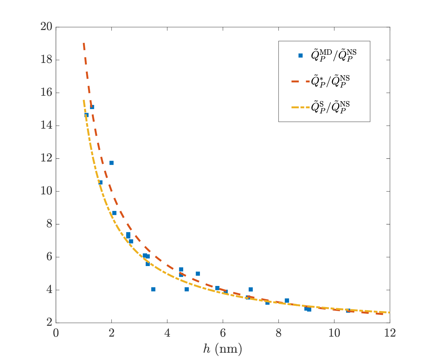
Figure 2: Flowrates for a range of channel heights $1.4\;\text{nm}\;\leq h\leq 10.8\;\text{nm}$. Comparison between the MD simulation results (denoted by $\tilde{Q}_{P}^{\rm MD}$) and expression (11) (denoted by $\tilde{Q}^{*}_{P}$). Expression (10) with $F=1$ and parameters $\mu=\hat{\mu}$ and $L_{s}=\hat{L}_{s}$ (slip flow with parameters extracted from large channels) is also shown and is denoted by ${Q}^{\rm S}_{P}$. All results are normalized by $\tilde{Q}_{P}^{\rm NS}$ (no-slip Navier-Stokes flowrate).

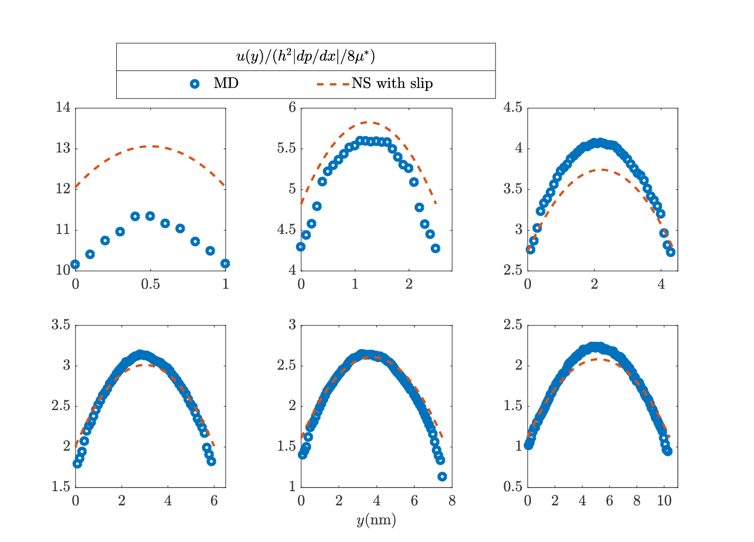
Figure 3: Normalized velocity profiles for films of different thicknesses in "pressure-driven" flow. Blue circles denote MD simulation data, while the red lines are the velocities predicted by slip-corrected Navier-Stokes with parameters $L_{s}^{*}$ and $\mu^{*}$. The channel widths considered in the figures $A$ to $F$ respectively are $1.4,2.9,4.8,6.4,7.8$ and $10.8\;{\rm nm}$.

3.2 The barrel drop problem

Figure 4 shows the "barrel drop" geometry used for validation of the ideas presented in this paper. In this problem, flow occurs due to the motion of the lower wall in the negative ${\bf\hat{x}}$ direction with velocity $U$, as assumed in the lubrication equation (8). The upper wall is stationary and of parabolic shape. Thus, the gap height as a function of the axial coordinate is given by $h(x)=h_{0}+a(x-L_{x}/2)^{2}$, where $L_{x}$ is the length of the domain in the ${\bf\hat{x}}$ direction.

Figure 4: A schematic model of the "barrel drop" lubrication geometry, which is used in the MD validation problem. $L_{x}$ is the size of the MD simulation box in the axial direction ${\bf\hat{x}}$. The section at $A$-$A^{\prime}$ shows the $x$-$z$ plane along which the pressure is measured using the method of planes [36] (See A.3).

In a general case, equation (8) would have to be solved numerically (say, using a Finite Volume scheme). In this case however, the simplicity of the barrel drop geometry and the constitutive relation (10) makes a semi-analytical solution for the pressure distribution possible. Using the fact that $\partial h/\partial t=0$, we integrate (8) once to obtain the constant volumetric flowrate

$$Q=-\frac{Uh(x)}{2}-\frac{dp}{dx}\tilde{Q}^{*}_{P}(h(x))$$ (12)

where $\tilde{Q}^{*}_{P}(h(x))$ is given in (11). Solving for the pressure, we obtain

$$p(x)=p_{0}-\int_{0}^{x}\frac{2Q+Uh(x^{\prime})}{\displaystyle\tilde{Q}^{*}_{P}(h(x^{\prime}))}\;dx^{\prime}$$ (13)

The flowrate $Q$ can be calculated from the following expression,

$$Q=-\dfrac{{\displaystyle\int_{0}^{L_{x}}}Uh(x^{\prime})[\tilde{Q}^{*}_{P}(h(x^{\prime}))]^{-1}dx^{\prime}}{\displaystyle{\int_{0}^{L_{x}}}2[\tilde{Q}^{*}_{P}(h(x^{\prime}))]^{-1}dx^{\prime}}$$ (14)

obtained on applying periodic boundary conditions $p(0)=p(L_{x})$ on the pressure. The constant $p_{0}$ can be calculated from the force balance

$$\int_{0}^{L_{x}}p(x)dx=N$$ (15)

where $N$ denotes the total normal force per unit depth (in the $z$ direction) acting on the top surface (assumed given). Due to the symmetry of the film thickness profile about $x=0$, the above relation reduces to [37]:

$$p_{0}L_{x}=N$$ (16)

Finally, the analytical pressure distribution can be obtained from (13), using $Q$ and $p_{0}$ from (14) and (16).

3.3 Results

In this section we compare the pressure distribution (13) against the corresponding MD result, denoted by $p^{\rm MD}$. Two such comparisons are performed here for different minimum gap heights ($h_{0}$). The first one is for a minimum gap height $h_{0}=3.8\;{\rm nm}$, while the second one is for $h_{0}=1.6\;{\rm nm}$. In the first comparison, shown in figure 5, $h_{0}$ is sufficiently large to avoid the presence of solvation and disjoining effects which make direct comparison of the pressure fields difficult. The pressure computed from the MD simulation agrees with the analytical pressure distribution closely. Here we recall that, according to our MD results, for $h\lesssim 6\;{\rm nm}$, $y$-resolved velocity profiles cannot be described by a fixed ($h$-independent) viscosity and slip-length, and thus a lubrication approach based on the traditional Reynolds equation would not be valid.

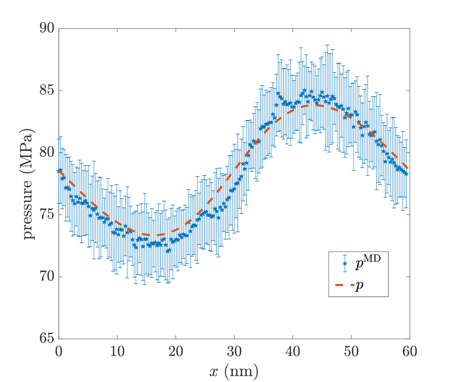
Figure 5: Comparison between the semi-analytical solution $p(x)$ given by (13) and the pressure computed from the MD simulation, $p^{\rm MD}(x)$, for the "barrel drop" problem with $h_{0}=3.8\;{\rm nm}$.

As stated above, validation at smaller gap heights is complicated by the appearance of solvation (structuring) and disjoining pressure effects [38, 39]. Disjoining pressure effects are caused by long-range (van der Waals) forces and have been considered in a variety of contexts, most notably wetting [40]. Solvation forces result from the entropic contribution of fluid layering at the wall [38]; as a result, they are important when the characteristic lengthscale $h$ is comparable to the layering thickness, that is, only under extreme confinement [39, 41].

Figure 6 shows $p^{\rm MD}$ for the barrel drop case with $h_{0}=1.6\;{\rm nm}$; although both solvation and disjoining effects are important at this scale, solvation effects are particularly evident in the regions corresponding to $h\lesssim 3\;{\rm nm}$ due to their distinctive oscillatory nature.

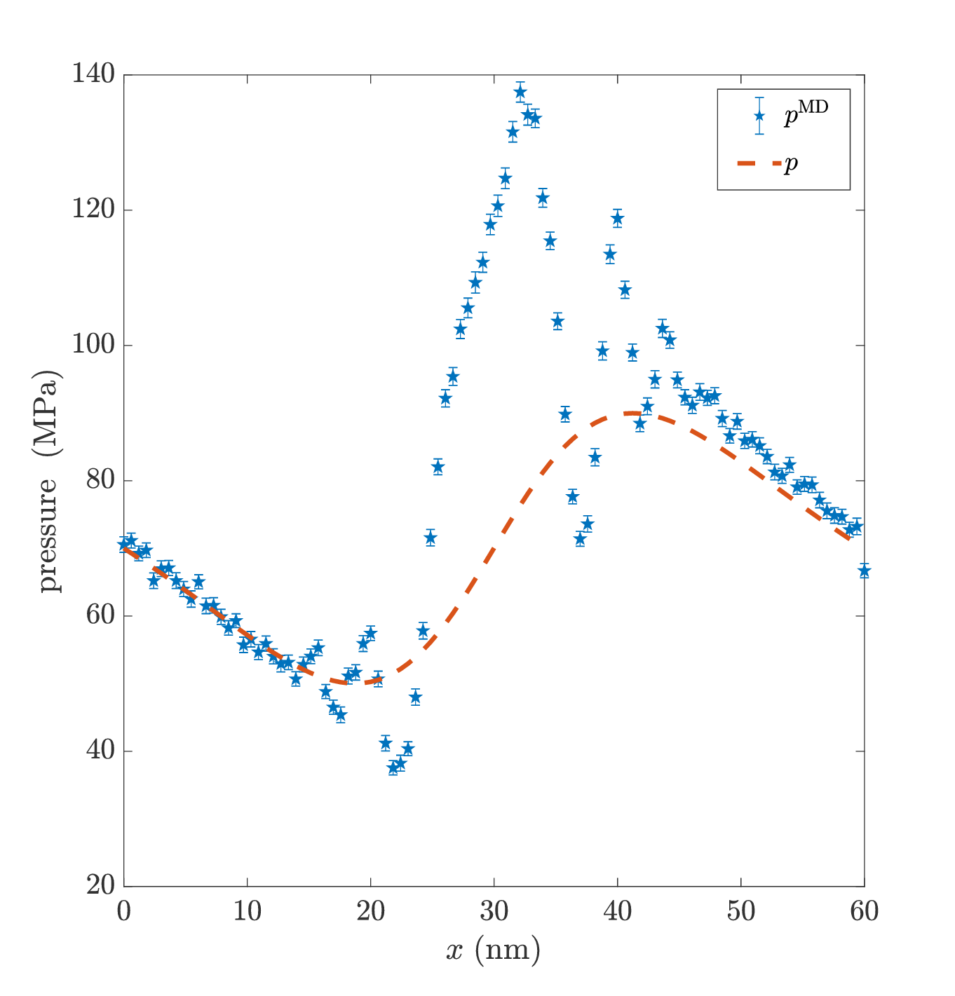
Figure 6: Comparison between the semi-analytical solution $p(x)$ given by (13) and the pressure computed from the MD simulation, $p^{\rm MD}(x)$, for the "barrel drop" problem with $h_{0}=1.6\;{\rm nm}$ As $h\rightarrow\hat{\sigma}$, disjoining and solvation effects become important. The latter are particularly apparent.

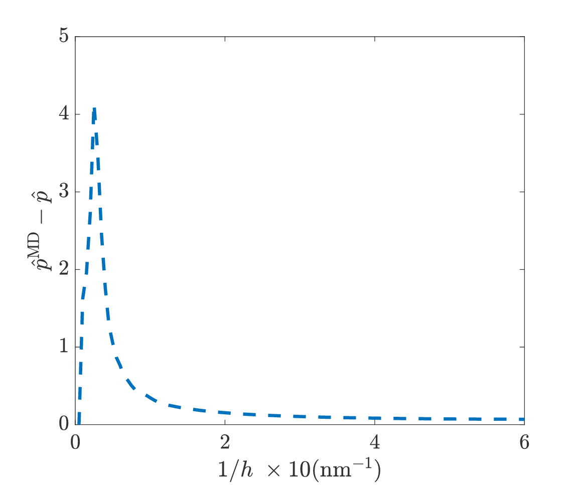
Figure 7: The Fourier transform of $p^{\rm MD}-p$ clearly shows a peak at $1/h=2.5$ (corresponding to $0.4\;{\rm nm}$), indicating the dominant wavelength associated with the spatial variation of solvation effects.

Solvation and disjoining pressure effects can be included in the proposed formulation by solving equation (8) subject to the boundary conditions $p(0)=p(L_{x})$ and

$$N=\int_{0}^{L_{x}}[p(x)+p_{s}(h(x))+p_{d}(h(x))]\;dx$$ (17)

where $p_{s}(h(x))$ denotes the solvation pressure and

$$p_{d}(h(x))=\frac{A}{6\pi h^{3}(x)}$$ (18)

is the disjoining pressure, where $A$ denotes the Hamaker constant [38].

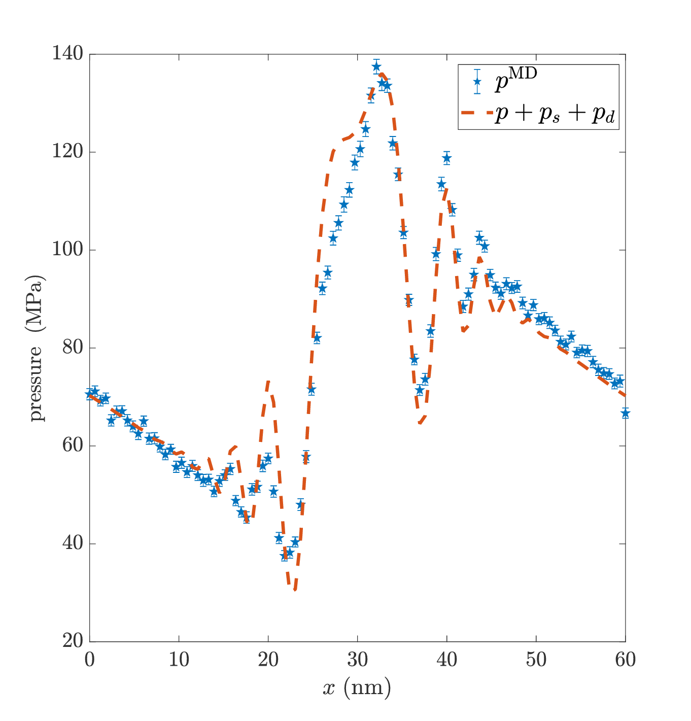
Figure 8: Comparison between $p(x)+p_{s}(h(x))+p_{d}(h(x))$, given by (13) and (20) respectively, and the pressure computed from the MD simulation, $p^{\rm MD}(x)$, for the "barrel drop" problem with $h_{0}=1.6\;{\rm nm}$.

It is important to note that although $p_{s}$ and $p_{d}$ are of $O(\varepsilon^{0})$, they are not included in the GLE (8) because, as discussed in section 2.1, the (local) flowrate $Q$ is calculated from the response to the zeroth-order balance (5), while

$$\frac{d}{dx}(p_{d}+p_{s})=\frac{d(p_{s}+p_{d})}{dh}\frac{dh}{dx}$$ (19)

is of order $\varepsilon^{1}$.

Although the molecular origin of the solvation pressure is well-understood [38, 42], reliable expressions for predicting its magnitude for various fluids are not available. However, Joly et al. [41] have recently shown that an expression of the form

$$p_{s}^{2D}(h(x)) =-\rho_{\infty}k_{B}T\cos{(2\pi h(x)/\delta)}\exp{(-h(x)/\delta)}.$$ (20)

developed for a hard-sphere fluid in two-dimensions, can be used to describe this effect in water, provided $\rho_{\infty}$, originally defined as the bulk fluid density far from the wall, was treated as an adjustable parameter. In the above expression, $\delta$ is a parameter related to the fluid structure and is thus expected to be of order $\hat{\sigma}$. We use $p_{s}^{\rm 2D}$ above to model $p_{s}$, with the value of $\delta$ and $\rho_{\infty}$ determined from our simulation data. To determine $\delta$ we use the Fourier transform of $p^{\rm MD}-p$, shown in figure 7, which exhibits a single peak at $0.4\;\rm{nm}$, confirming the sinusoidal dependence of $p_{s}$ on $h$ and suggesting $\delta=0.4\;{\rm nm}$. This value is known from surface-force measurements and MD simulations [43, 44] to be close to the thickness of a layer of n-hexadecane confined between crystalline substrates.

Using this value for $\delta$ and treating $\rho_{\infty}$ as an adjustable (fitting) constant, we show in figure 8 that the decomposition $p+p_{s}+p_{d}$ can model $p^{\rm MD}$ for $h$ as low as $1.6\;{\rm nm}$.

4 Discussion and Conclusions

We have discussed a Generalized Lubrication Equation framework for the solution of dense-fluid lubrication problems at the nanometer scale. The framework is based on the observation that under the lubrication approximation, the closure required is significantly less difficult to obtain than for the general flow case.

In the example considered here, it was assumed that the two solid surfaces interact with the fluid identically and thus the Couette component of the flowrate, by symmetry, remains equal to its Navier-Stokes no-slip value. The proposed methodology can be extended to cases where interactions are asymmetric by developing a constitutive relation for the Couette component of the flowrate. Although in the example lubricant-wall model studied here the flowrate was reproduced using a slip-flow-based relationship, the GLE is in no way reliant on the validity of a slip-flow description. As an example, see the dilute gas case (eq. (9)) and the related discussion in section 2.2. Developing a general scaling relation for $\tilde{Q}_{P}$ in terms of the governing molecular parameters for dense fluids is the subject of future work, although significant progress has been made for particular fluid-solid systems (see section 1). Such a relation would potentially reduce the number of simulations/experiments required to describe $\tilde{Q}_{P}(A,h,\rho,T,B)$ for a particular fluid.

Developing a constitutive relation and solving the resulting GLE is considerably more tractable than brute-force MD simulations for problems of practical interest. In fact, the latter is usually impossible, both because of the cost associated with the number of particles required for such simulations, but also because the characteristic timescales of such systems are much longer. For example, the cost associated with the GLE (primarily MD simulations for constructing the constitutive relation) is smaller (approximately by a factor of 2) than the cost of one barrel drop simulation, even though the latter is at lengthscales much smaller than actual problems of practical interest (deliberately chosen for validation purposes, to ensure that an MD solution was feasible). Once the constitutive relation is developed, additional solutions of the GLE come at a cost that is essentially negligible (compared to MD simulations).

For very small film heights, solvation and disjoining effects become important. Fortunately, as in previous work [41, 39], it was shown that these effects can be satisfactorily accounted for by linearly superposing their contribution to the hydrodynamic pressure, requiring minimal modification of the lubrication equation. Although in both cases (present and previous work [41]) good agreement with MD simulations was found by fitting the result for hard-spheres in two dimensions, it is clear that our ability to model solvation effects for more realistic fluids is very limited and needs to be improved.

5 Acknowledgments

The authors would like to thank Mathew Swisher and Gerald J. Wang for help with the computations and many helpful comments and suggestions during the course of this research. This work was sponsored by the Consortium on Lubrication in Internal Combustion Engines with additional support from Argonne National Laboratory and the US Department of Energy. The current consortium members are Daimler, Mahle, MTU Friedrichshafen, PSA Peugeot Citroën, Renault, Shell, Toyota, Volkswagen, Volvo Cars, Volvo Trucks, and Weichai Power. The use of the Center for Nanoscale Materials, an Office of Science user facility, was supported by the U. S. Department of Energy, Office of Science, Office of Basic Energy Sciences, under Contract No. DE-AC02-06CH11357.

This is a pre-print of an article published in Microfluidics and Nanofluidics.

Appendix A MD simulations

All MD simulations in this work were performed using the software package LAMMPS [45].

As explained in section 2.2, the constitutive relation was developed by studying fully-developed flow in two-dimensional channels. The validation was performed in the barrel drop geometry of figure 4, which is a significantly larger scale problem. In both cases, the model lubricant is n-hexadecane, simulated using the TraPPE potential [46], while the system solid boundaries are atomically smooth iron (BCC Fe) walls, simulated using the Embedded Atom Method - Finnis Sinclair [47, 48, 49] potential. The Lennard-Jones (LJ) parameters used between well-separated pseudo-atoms, i.e, a pair of pseudo-atoms separated by 3 or more pseudo-atoms within the same molecule or a pair belonging to two different molecules within the fluid are given in table 1. The LJ parameters of interaction between atoms of unlike types were calculated using the Lorentz-Berthelot mixing rules.

Bond stretching in the fluid molecules was modelled via a harmonic potential of the form, $\displaystyle U_{ij}=\frac{k_{r}}{2}(r_{ij}-r_{0})^{2}$, where $r_{0}=1.54\;\text{\AA}$ is the equilibrium bond length and $k_{r}$, the bond stretching parameter taken here to have the value $19.5139\;{\rm eV/\text{\AA}}^{2}$ (chosen from Lopez-Lemus et al [50]). The bending energy associated with variations of the angle between 3 adjacent atoms connected through bonds was modelled through a harmonic potential [46] of the form $\displaystyle U_{{\rm bend}}=\frac{k_{\theta}}{2}(\theta-\theta_{0})^{2}$, where the bending parameter $k_{\theta}$ is taken as $2.6925\;{\rm eV}$ and the equilibrium angle, $\theta_{0}=114^{\circ}$. The torsional potential that arises due to the bending of the dihedral angle, $\phi$, was given by an OPLS style potential [51] : $\displaystyle U_{{\rm torsion}}=\frac{c_{1}}{2}(1+\cos\phi)+\frac{c_{2}}{2}(1-\cos(2\phi))+\frac{c_{3}}{2}(1+\cos(3\phi))$. The parameters were taken from Martin et al. [46] to be:

$$c_{1}=0.05774\quad c_{2}=-0.0117524,\quad c_{3}=0.136382$$

Type of pseudo-atom $i$	Type of pseudo-atom $j$	$\sigma$(Å)	$\epsilon$(eV)
$CH_{2}$	$CH_{2}$	3.95	0.003964
$CH_{3}$	$CH_{3}$	3.75	0.008445
$CH_{3}$	$CH_{2}$	3.85	0.0058
$Fe$	Fe	2.2	0.02947

Table 1: The LJ parameters of interaction between different atomic species used in the paper.

The interactions between the solid and the liquid atoms were modeled the LJ potential. The parameters for the wall-fluid interaction potential were computed through the Lorentz-Berthelot mixing rules, using the self-interaction parameters listed in table 1. Note that the self-interaction parameters for Fe were taken from Berro et al [8] (developed for more realistic simulation of Fe oxide surfaces) and are different from those reported in the literature for BCC Fe (see Zhen et al. [52], for example).

A.1 Channel flow

The simulations were performed in channels of length $99.94\;\text{\AA}$ in the flow direction, ${\bf\hat{x}}$, and width $71.38\;\text{\AA}$, in the ${\bf\hat{z}}$ direction. The channel width in the transverse ${\bf\hat{y}}$ direction, denoted by $h$, varied between $1.4\;{\rm nm}$ and $10.8\;{\rm nm}$. Fluid motion was generated by applying a body force per unit mass in the flow direction, $g$, while periodic boundary conditions were imposed in the flow direction, ${\bf\hat{x}}$, thus eliminating entrance effects and making the flow fully developed by construction. Periodic boundary conditions were also applied in the homogeneous (depth) direction, ${\bf\hat{z}}$. In the transverse, ${\bf\hat{y}}$, direction, the fluid was bounded by two solid walls. Each wall consisted of eight layers of atomically smooth BCC Fe (001) surface, of thickness $22.84\;\text{\AA}$. The two layers furthest away from the fluid were frozen (using LAMMPS’s fix rigid) and provided the wall structure; the adjacent three layers of atoms were responsible for maintaining the simulation temperature at 450 K and were thus thermostatted using a Nosé-Hoover thermostat. No constraints were imposed on the three layers closest to the liquid. The fluid pressure was maintained at 80 MPa, by applying a normal force (in the negative ${\bf\hat{y}}$ direction) to the frozen solid layers. To avoid thermostat-induced artifacts [53], no thermostat was applied to the fluid molecules during the data sampling phase (a Langevin thermostat was used for the initial equilibration phase). Viscous heat generated within the fluid was removed by the thermostatted wall molecules. To ensure small temperature variations, the maximum fluid velocity was on the order of 50 m/s or less, resulting in a maximum temperature variation of $O$(5K), which is sufficiently small for the isothermal assumption to be valid. We have determined empirically that taking the body force to be sufficiently small so that temperature variations were small (and thus non-linearities due to temperature-dependent transport coefficients were negligible) also ensured linear response, for which pressure-driven and body-force-driven flow are expected to be equivalent. This equivalence was validated by our results of section 3.1. We also note that actual flow speeds encountered in nanoscale flows are much smaller (usually by many orders of magnitude) than the flow velocities used here (which are large in order to improve signal to noise ratio [54]); in other words, isothermal flow and linear response assumptions are even more justified for real flows.

Simulation results are shown in figures 2 and 3 and discussed in section 3.1. In figure 3, $|dp/dx|$ represents the "effective pressure gradient magnitude" ($=\rho g$).

A.2 Barrel drop

The geometry of the barrel drop profile is shown in figure 4. Fluid flow was generated by the motion of the lower solid boundary at a speed of $U=60\;{\rm m/s}$. Both the upper parabolic surface and the lower plane surface consisted of rigid, thermostat and deformable layers, with constraints (including thermostating) analogous to those discussed in the previous section on channel flow. Specifically, heat was removed from the system by thermostating the three wall layers furthest away from the fluid in each wall, and no thermostat was applied to the fluid during the data sampling phase. The extent of the simulation box in the two lateral directions, ${\bf\hat{x}}$ and ${\bf\hat{z}}$, was $L_{x}=59.9\;{\rm nm}$ and $L_{z}=25.6\;{\rm nm}$, respectively. Based on a characteristic lengthscale $L_{c}=40\;{\rm nm}$, the non-dimensional value of the curvature parameter is $aL_{c}^{2}/h_{0}=1.845$.

A.3 Computation of pressure in MD simulations

As is well known from previous work [36, 55, 56], the Irving-Kirkwood (IK) formula for the stress tensor in a fluid exhibits spurious oscillations near hard system boundaries such as solid walls. As a result, in the present work the fluid pressure is measured by calculating the $p_{yy}$ component of the configurational part of the stress tensor, as the sum of all molecular forces acting across a flat (imaginary) dividing plane whose normal is in the ${\bf\hat{y}}$ direction. Specifically, we are using an approach known as the Method of Planes (MOP) [55], in which the configurational part of the stress tensor at location $y$ is calculated by

$$p_{yy}^{c}(y) =\frac{1}{4A}\sum_{ij}F_{ij}^{y}\Bigg{(}{\rm sgn}(y_{i}-y)-{\rm sgn}(y_{j}-y)\Bigg{)}$$ (21)

where $y_{i}$ and $y_{j}$ are the components of the position vectors of atoms $i$ and $j$ in the ${\bf\hat{y}}$ direction at time $t$, respectively, and $F_{ij}^{y}$ represents the ${\bf\hat{y}}$-component of the force on atom $i$ due to atom $j$. The force component $F_{ij}^{y}$ contributes to the configurational pressure only if it acts across the plane at $y$. The pressure is then given by $p=p_{yy}$; we have independently verified, via simulations in 2D channels that the stress tensor remains isotropic even at these small scales. The above definition assumes pairwise forces between contributing atoms. Stress tensor definitions for systems of particles interacting through many-body forces have only been developed for the virial IK-based formulation [57]. To overcome this limitation, here we use the fact that, in the lubrication approximation, the fluid pressure is independent of $y$. We have thus placed the sampling plane in the narrow gap between wall and liquid, which ensures that any pair of contributing atoms is never both solid or liquid. An additional benefit associated with this choice is that no atom-crossings occur across this sampling plane, meaning that the kinetic term

$$p_{yy}^{k}(y) =\frac{1}{2A}\sum_{i}m_{i}v_{i}\frac{d}{dt}{\rm sgn}(y_{i}-y).$$ (22)

does not contribute. In the above equation, $m_{i}$ is the mass of particle $i$ and $v_{i}$ is the component of the particle velocity of particle $i$ in the ${\bf\hat{y}}$ direction at time $t$.

Although derived for infinitely large planes, in the case of the barrel drop geometry, in order to resolve the pressure variation in the flow direction, we have applied expression (21) locally, that is, over bins of finite extent in the flow (${\bf\hat{x}}$) direction. The number of bins was chosen to balance the need for good axial resolution of the pressure with the need for the number of bins to be as small as possible so that the change in pressure across consecutive bins is small. Specifically, we used 100 bins, with each bin spanning $0.6\;{\rm nm}$ in the ${\bf\hat{x}}$ direction and the size of the periodic box, $25.6\;{\rm nm}$, in the ${\bf\hat{z}}$ direction.

References

- Allen and Tildesley [1989] M. P. Allen, D. J. Tildesley, Computer simulation of liquids, Oxford university press, 1989.
- Frenkel and Smit [2002] D. Frenkel, B. Smit, Understanding molecular simulation: from algorithms to applications, volume 1, Elsevier (formerly published by Academic Press), 2002.
- Mattia et al. [2015] D. Mattia, H. Leese, K. P. Lee, Carbon nanotube membranes: from flow enhancement to permeability, Journal of Membrane Science 475 (2015) 266–272.
- Guo et al. [2015] S. Guo, E. R. Meshot, T. Kuykendall, S. Cabrini, F. Fornasiero, Nanofluidic transport through isolated carbon nanotube channels: Advances, controversies, and challenges, Advanced Materials 27 (2015) 5726–5737.
- Secchi et al. [2016] E. Secchi, S. Marbach, A. Niguès, D. Stein, A. Siria, L. Bocquet, Massive radius-dependent flow slippage in carbon nanotubes, Nature 537 (2016) 210–213.
- Popadić et al. [2014] A. Popadić, J. H. Walther, P. Koumoutsakos, M. Praprotnik, Continuum simulations of water flow in carbon nanotube membranes, New Journal of Physics 16 (2014).
- Zheng et al. [2013] X. Zheng, H. Zhu, B. Kosasih, A. K. Tieu, A molecular dynamics simulation of boundary lubrication: The effect of n-alkanes chain length and normal load, Wear 301 (2013) 62–69.
- Berro et al. [2010] H. Berro, N. Fillot, P. Vergne, Molecular dynamics simulation of surface energy and ZDDP effects on friction in nano-scale lubricated contacts, Tribology International 43 (2010) 1811–1822.
- Savio et al. [2013] D. Savio, N. Fillot, P. Vergne, A molecular dynamics study of the transition from ultra-thin film lubrication toward local film breakdown, Tribology Letters 50 (2013) 207–220.
- Zheng et al. [2013] X. Zheng, H. Zhu, A. K. Tieu, B. Kosasih, A molecular dynamics simulation of 3d rough lubricated contact, Tribology international 67 (2013) 217–221.
- Landman et al. [1996] U. Landman, W. D. Luedtke, J. Gao, Atomic-scale issues in tribology: interfacial junctions and nano-elastohydrodynamics, Langmuir 12 (1996) 4514–4528.
- Priezjev et al. [2005] N. V. Priezjev, A. A. Darhuber, S. M. Troian, Slip behavior in liquid films on surfaces of patterned wettability: Comparison between continuum and molecular dynamics simulations, Physical Review E 71 (2005) 041608.
- Ghorbanian et al. [2016] J. Ghorbanian, A. T. Celebi, A. Beskok, A phenomenological continuum model for force-driven nano-channel liquid flows, The Journal of Chemical Physics 145 (2016) 184109.
- Travis et al. [1997] K. P. Travis, B. D. Todd, D. J. Evans, Departure from Navier-Stokes hydrodynamics in confined fluids, Physical Review E 55 (1997) 4288–4295.
- Sofos et al. [2009] F. Sofos, T. Karakasidis, A. Liakopoulos, Transport properties of liquid argon in krypton nanochannels: Anisotropy and non-homogeneity introduced by the solid walls, International Journal of Heat and Mass Transfer 52 (2009) 735–743.
- Ghorbanian and Beskok [2016] J. Ghorbanian, A. Beskok, Scale effects in nano-channel liquid flows, Microfluidics and Nanofluidics 20 (2016) 121.
- Hadjiconstantinou [2006] N. G. Hadjiconstantinou, The limits of Navier-Stokes theory and kinetic extensions for describing small-scale gaseous hydrodynamics, Physics of Fluids 18 (2006) 111301.
- Fukui and Kaneko [1988] S. Fukui, R. Kaneko, Analysis of ultra-thin gas film lubrication based on linearized Boltzmann equation: First report- derivation of a generalized lubrication equation including thermal creep flow, Journal of Tribology 110 (1988) 253–261.
- Leal [2007] L. G. Leal, Advanced transport phenomena: fluid mechanics and convective transport processes, Cambridge University Press, 2007.
- Szeri [2011] A. Z. Szeri, Fluid film lubrication, Cambridge University Press, 2011.
- Alexander et al. [1994] F. J. Alexander, A. L. Garcia, B. J. Alder, Direct Simulation Monte Carlo for thin-film bearings, Physics of Fluids 6 (1994) 3854–3860.
- Gallis and Torczynski [2004] M. A. Gallis, J. R. Torczynski, An improved Reynolds-equation model for gas damping of microbeam motion, Journal of Microelectromechanical systems 13 (2004) 653–659.
- Cercignani [2006] C. Cercignani, Slow rarefied flows: Theory and application to Micro-Electro-Mechanical systems, volume 41, Springer Science & Business Media, 2006.
- Fillot et al. [2011] N. Fillot, H. Berro, P. Vergne, From continuous to molecular scale in modelling elastohydrodynamic lubrication: Nanoscale surface slip effects on film thickness and friction, Tribology Letters 43 (2011) 257–266.
- Savio et al. [2015] D. Savio, N. Fillot, P. Vergne, H. Hetzler, W. Seemann, G. M. Espejel, A multiscale study on the wall slip effect in a ceramic–steel contact with nanometer-thick lubricant film by a nano-to-elastohydrodynamic lubrication approach, Journal of Tribology 137 (2015) 031502.
- Savio et al. [2016] D. Savio, L. Pastewka, P. Gumbsch, Boundary lubrication of heterogeneous surfaces and the onset of cavitation in frictional contacts, Science Advances 2 (2016) e1501585.
- Borg et al. [2013] M. K. Borg, D. A. Lockerby, J. M. Reese, A multiscale method for micro/nano flows of high aspect ratio, Journal of Computational Physics 233 (2013) 400–413.
- Ren and Weinan [2005] W. Ren, E. Weinan, Heterogeneous multiscale method for the modeling of complex fluids and micro-fluidics, Journal of Computational Physics 204 (2005) 1–26.
- Yoshida and Bocquet [2016] H. Yoshida, L. Bocquet, Labyrinthine water flow across multilayer graphene-based membranes: Molecular dynamics versus continuum predictions, The Journal of Chemical Physics 144 (2016) 234701.
- Schlaich et al. [2017] A. Schlaich, J. Kappler, R. R. Netz, Hydration friction in nanoconfinement: From bulk via interfacial to dry friction, Nano letters 17 (2017) 5969–5976.
- Holland et al. [2015] D. M. Holland, D. A. Lockerby, M. K. Borg, W. D. Nicholls, J. M. Reese, Molecular dynamics pre-simulations for nanoscale computational fluid dynamics, Microfluidics and Nanofluidics 18 (2015) 461–474.
- Wang and Hadjiconstantinou [2017] G. J. Wang, N. G. Hadjiconstantinou, Molecular mechanics and structure of the fluid-solid interface in simple fluids, Physical Review Fluids 2 (2017) 094201.
- Wang and Hadjiconstantinou [2015] G. J. Wang, N. G. Hadjiconstantinou, Why are fluid densities so low in carbon nanotubes?, Physics of Fluids 27 (2015) 052006.
- Cameron [1983] A. Cameron, Basic lubrication theory, Ellis Horwood Ltd., 1983.
- Burgdorfer [1959] A. Burgdorfer, The influence of the molecular mean free path on the performance of hydrodynamic gas lubricated bearings, ASME Journal of Basic Engineering 81 (1959).
- Cheung and Yip [1991] K. S. Cheung, S. Yip, Atomic-level stress in an inhomogeneous system, Journal of Applied Physics 70 (1991) 5688–5690.
- Chandramoorthy [2016] N. Chandramoorthy, Molecular dynamics-based approaches for mesoscale lubrication, Master’s thesis, Massachusetts Institute of Technology, 2016.
- Israelachvili [2011] J. Israelachvili, Intermolecular and surface forces, Elsevier, 2011.
- Kato and Matsuoka [1999] T. Kato, H. Matsuoka, Molecular layering in thin-film elastohydrodynamics, Proceedings of the Institution of Mechanical Engineers, Part J: Journal of Engineering Tribology 213 (1999) 363–370.
- De Gennes [1985] P.-G. De Gennes, Wetting: statics and dynamics, Reviews of modern physics 57 (1985) 827.
- Gravelle et al. [2016] S. Gravelle, C. Ybert, L. Bocquet, L. Joly, Anomalous capillary filling and wettability reversal in nanochannels, Physical Review E 93 (2016) 033123.
- Henderson [1986] J. Henderson, Compressibility route to solvation structure, Molecular Physics 59 (1986) 89–96.
- Ribarsky and Landman [1992] M. W. Ribarsky, U. Landman, Structure and dynamics of n-alkanes confined by solid surfaces. i. stationary crystalline boundaries, The Journal of Chemical Physics 97 (1992) 1937–1949.
- Christenson et al. [1987] H. Christenson, D. Gruen, R. Horn, J. Israelachvili, Structuring in liquid alkanes between solid surfaces: Force measurements and mean-field theory, The Journal of chemical physics 87 (1987) 1834–1841.
- Plimpton [1995] S. Plimpton, Fast parallel algorithms for short-range molecular dynamics, Journal of Computational Physics 117 (1995) 1–19.
- Martin and Siepmann [1999] M. G. Martin, J. I. Siepmann, Novel configurational-bias Monte Carlo method for branched molecules. Transferable Potentials for Phase Equilibria. 2. United-Atom description of branched alkanes, The Journal of Physical Chemistry B 103 (1999) 4508–4517.
- Mendelev and et al [2010] M. I. Mendelev, et al, Interatomic potentials repository project, http://www.ctcms.nist.gov/potentials/Download/Fe-MIM2/Fe_2.eam.fs, 2010. Updated on 22 Dec 2010.
- Mendelev et al. [2003] M. I. Mendelev, S. Han, D. J. Srolovitz, G. J. Ackland, D. Y. Sun, Development of new interatomic potentials appropriate for crystalline and liquid Iron, Philosophical Magazine 83 (2003) 3977–3994.
- Ackland et al. [1997] G. J. Ackland, D. J. Bacon, A. F. Calder, T. Harry, Computer simulation of point defect properties in dilute Fe-Cu alloy using a many-body interatomic potential, Philosophical Magazine A 75 (1997) 713–732.
- Lòpez-Lemus et al. [2006] J. Lòpez-Lemus, M. Romero-Bastida, T. A. Darden, J. Alejandre, Liquid-vapour equilibrium of n-alkanes using interface simulations, Molecular Physics 104 (2006) 2413–2421.
- Watkins and Jorgensen [2001] E. K. Watkins, W. L. Jorgensen, Perfluoroalkanes: Conformational analysis and liquid-state properties from ab initio and Monte Carlo calculations, The Journal of Physical Chemistry A 105 (2001) 4118–4125.
- Zhen and Davies [1983] S. Zhen, G. J. Davies, Calculation of the Lennard-Jones n-m potential energy parameters for metals, Physica Status Solidi (a) 78 (1983) 595–605.
- Pahlavan and Freund [2011] A. A. Pahlavan, J. B. Freund, Effect of solid properties on slip at a fluid-solid interface, Physical Review E 83 (2011) 021602.
- Hadjiconstantinou et al. [2003] N. G. Hadjiconstantinou, A. L. Garcia, M. Z. Bazant, G. He, Statistical error in particle simulations of hydrodynamic phenomena, Journal of Computational Physics 187 (2003) 274–297.
- Todd et al. [1995] B. Todd, D. J. Evans, P. J. Daivis, Pressure tensor for inhomogeneous fluids, Physical Review E 52 (1995) 1627.
- Cleri [2001] F. Cleri, Representation of mechanical loads in molecular dynamics simulations, Physical review B 65 (2001) 014107.
- Thompson et al. [2009] A. P. Thompson, S. J. Plimpton, W. Mattson, General formulation of pressure and stress tensor for arbitrary many-body interaction potentials under periodic boundary conditions, The Journal of Chemical Physics 131 (2009).