Sparse non-negative super-resolution — simplified and stabilised

Abstract

The convolution of a discrete measure, $x=\sum_{i=1}^{k}a_{i}\delta_{t_{i}}$, with a local window function, $\phi(s-t)$, is a common model for a measurement device whose resolution is substantially lower than that of the objects being observed. Super-resolution concerns localising the point sources $\{a_{i},t_{i}\}_{i=1}^{k}$ with an accuracy beyond the essential support of $\phi(s-t)$, typically from $m$ samples $y(s_{j})=\sum_{i=1}^{k}a_{i}\phi(s_{j}-t_{i})+\delta_{j}$, where $\delta_{j}$ indicates an inexactness in the sample value. We consider the setting of $x$ being non-negative and seek to characterise all non-negative measures approximately consistent with the samples. We first show that $x$ is the unique non-negative measure consistent with the samples provided the samples are exact, i.e. $\delta_{j}=0$, $m\geq 2k+1$ samples are available, and $\phi(s-t)$ generates a Chebyshev system. This is independent of how close the sample locations are and does not rely on any regulariser beyond non-negativity; as such, it extends and clarifies the work by Schiebinger et al. in [1] and De Castro et al. in [2], who achieve the same results but require a total variation regulariser, which we show is unnecessary.

Moreover, we characterise non-negative solutions $\hat{x}$ consistent with the samples within the bound $\sum_{j=1}^{m}\delta_{j}^{2}\leq\delta^{2}$. Any such non-negative measure is within ${\mathcal{O}}(\delta^{1/7})$ of the discrete measure $x$ generating the samples in the generalised Wasserstein distance. Similarly, we show using somewhat different techniques that the integrals of $\hat{x}$ and $x$ over $(t_{i}-\epsilon,t_{i}+\epsilon)$ are similarly close, converging to one another as $\epsilon$ and $\delta$ approach zero. We also show how to make these general results, for windows that form a Chebyshev system, precise for the case of $\phi(s-t)$ being a Gaussian window. The main innovation of these results is that non-negativity alone is sufficient to localise point sources beyond the essential sensor resolution and that, while regularisers such as total variation might be particularly effective, they are not required in the non-negative setting.

To David L. Donoho, a uniquely positive gentleman,
in celebration of his 60th birthday and with thanks for his inspiration and support.

1 Introduction

Super-resolution concerns recovering a resolution beyond the essential size of the point spread function of a sensor. For instance, a particularly stylised example concerns multiple point sources which, because of the finite resolution or bandwidth of the sensor, may not be visually distinguishable. Various instances of this problem exist in applications such as astronomy [3], imaging in chemistry, medicine and neuroscience [4, 5, 6, 7, 8, 9, 10, 11], spectral estimation [12, 13], geophysics [14], and system identification [15]. Often in these application much is known about the point spread function of the sensor, or can be estimated and, given such model information, it is possible to identify point source locations with accuracy substantially below the essential width of the sensor point spread function. Recently there has been substantial interest from the mathematical community in posing algorithms and proving super-resolution guarantees in this setting, see for instance [16, 17, 18, 19, 20, 21, 22, 23]. Typically these approaches borrow notions from compressed sensing [24, 25, 26]. In particular, the aforementioned contributions to super-resolution consider what is known as the Total Variation norm minimisation over measures which are consistent with the samples. In this manuscript we show first that, for suitable point spread functions, such as the Gaussian, any discrete non-negative measure composed of $k$ point sources is uniquely defined from $2k+1$ of its samples, and moreover that this uniqueness is independent of the separation between the point sources. We then show that by simply imposing non-negativity, which is typical in many applications, any non-negative measure suitably consistent with the samples is similarly close to the discrete non-negative measure which would generate the noise free samples. These results substantially simply results by [1, 2] and show that, while regularisers such as Total Variation may be particularly effective, in the setting of non-negative point sources such regularisers are not necessary to achieve stability.

1.1 Problem setup

Throughout this manuscript we consider non-negative measures in relation to discrete measures. To be concrete, let $x$ be a $k$-discrete non-negative Borel measure supported on the interval $I=[0,1]\subset\mathbb{R}$, given by

$$x=\sum_{i=1}^{k}a_{i}\cdot\delta_{t_{i}}\quad\mbox{with}\;\;a_{i}>0\quad\mbox{ and }t_{i}\in int(I)\quad\mbox{ for all }i.$$ (1)

Consider also real-valued and continuous functions $\{\phi_{j}\}_{j=1}^{m}$ and let $\{y_{j}\}_{j=1}^{m}$ be the possibly noisy measurements collected from $x$ by convolving against sampling functions $\phi_{j}(t)$:

$$y_{j}=\int_{I}\phi_{j}(t)x(\operatorname{d\!}t)+\delta_{j}=\sum_{i=1}^{k}a_{i}\phi_{j}(t_{i})+\delta_{j},$$ (2)

where $\delta_{j}$ with $\sum_{j=1}^{m}\delta_{j}^{2}\leq\delta^{2}$ can represent additive noise. Organising the $m$ samples from (2) in matrix notation by letting

$$y\mathrel{\mathop{\mathchar 58\relax}}=[y_{1}\;\cdots\;y_{m}]^{T}\in{\mathbb{R}}^{m},\quad\quad\Phi(t)\mathrel{\mathop{\mathchar 58\relax}}=[\phi_{1}(t)\;\cdots\;\phi_{m}(t)]^{T}\in{\mathbb{R}}^{m}$$ (3)

allows us to state the program we investigate:

$$\text{find }z\geq 0\text{ subject to }\left\|y-\int_{I}\Phi(t)z(\operatorname{d\!}t)\right\|_{2}\leq\delta^{\prime},$$ (4)

with $\delta\leq\delta^{\prime}$. Herein we characterise non-negative measures consistent with measurements (2) in relation to the discrete measure (1). That is, we consider any non-negative Borel measure $z$ from the Program (4) and show that any such $z$ is close to $x$ given by (1) in an appropriate metric, see Theorems 4, 5, 11, 12 and 13. Note that when solving Program (4), the measure $x$ is completely unkown, so neither the source locations $\{t_{i}\}_{i=1}^{k}$ and weights $\{a_{i}\}_{i=1}^{k}$ nor their number $k$ is known in advance. Moreover, we show that the $x$ from (1) is the unique solution to Program (4) when $\delta^{\prime}=0$; e.g. in the setting of exact samples, $\eta_{i}=0$ for all $i$. Program (4) is particularly notable in that there is no regulariser of $z$ beyond imposing non-negativity and, rather than specify an algorithm to select a $z$ which satisfies Program (4), we consider all admissible solutions. The aim of doing this is to highlight that non-negativity is the main regulariser, especially in the noise-free setting. However, a practitioner solving this problem in the context of sparse measures would be advised to include additional regularisers such as the TV norm or a sparsity constraint in the context of non-convex methods to encourage sparisty, specifically in the noisy setting.

The admissible solutions of Program (4) are determined by the source and sample locations, which we denote as

$$T=\{t_{i}\}_{i=1}^{k}\subset\operatorname{int}(I)\quad\text{ and }\quad S=\{s_{j}\}_{j=1}^{m}\subseteq I$$ (5)

respectively, as well as the particular functions $\phi_{j}(t)$ used to sample the $k$-sparse non-negative measure $x$ from (1). Lastly, we introduce the notions of minimum separation and sample proximity, which we use to characterise solutions of Program (4).

Definition 1.

(Minimum separation and sample proximity) For finite $\tilde{T}=T\cup\{0,1\}\subset I$, let $\Delta(T)>0$ be the minimum separation between the points in $T$ along with the endpoints of $I$, namely

$$\Delta(T)=\min_{T_{i},T_{j}\in\tilde{T},i\neq j}|T_{i}-T_{j}|.$$ (6)

We define the sample proximity to be the number $\lambda\in(0,\frac{1}{2})$ such that, for each source location $t_{i}$, there exists a closest sample location $s_{l(i)}\in S$ to $t_{i}$ with

$$|t_{i}-s_{l(i)}|\leq\lambda\Delta(T).$$ (7)

We describe the nearness of solutions to Program (4) in terms of an additional parameter $\epsilon$ associated with intervals around the sources $T$; that is we let $\epsilon\leq\Delta(T)/2$ and define intervals as:

$$T_{i,\epsilon}\mathrel{\mathop{\mathchar 58\relax}}=\left\{t\mathrel{\mathop{\mathchar 58\relax}}\left|t-t_{i}\right|\leq\epsilon\right\}\cap I,\qquad i\in[k],\quad T_{\epsilon}\mathrel{\mathop{\mathchar 58\relax}}=\bigcup_{i=1}^{k}T_{i,\epsilon},$$ (8)

where $[k]={1,2,\ldots,k}$, and set $T_{i,\epsilon}^{C}$ and $T_{\epsilon}^{C}$ to be the complements of these sets with respect to $I$. In order to make the most general result of Theorems 11 and 12 more interpretable, we turn to presenting them in Section 1.2 for the case of $\phi_{j}(t)$ being shifted Gaussians.

1.2 Main results simplified to Gaussian window

In this section we consider $\phi_{j}(t)$ to be shifted Gaussians with centres at the source locations $s_{j}$, specifically

$$\phi_{j}(t)=g(t-s_{j})=e^{-\frac{(t-s_{j})^{2}}{\sigma^{2}}}.$$ (9)

We might interpret (9) as the “point spread function” of the sensing mechanism being a Gaussian window and $s_{j}$ the sample locations in the sense that

$$\int_{I}\phi_{j}(t)x(\operatorname{d\!}t)=\int_{I}g(t-s_{j})x(\operatorname{d\!}t)=(g\star x)(s_{j}),\qquad\forall j\in[m],$$ (10)

evaluates the “filtered” copy of $x$ at locations $s_{j}$ where $\star$ denotes convolution.

As an illustration, Figure 1 shows the discrete measure $x$ in blue for $k=3$, the continuous function $y(s)=(g\star x)(x)$ in red, and the noisy samples $y(s_{j})$ at the sample locations $S$ represented as the black circles.

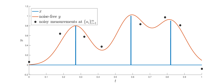
Figure 1: Example of discrete measure $x$ and measurements where $\phi_{j}(t)=\phi(t-s_{j})$ for $s_{j}\in S$ and the Gaussian kernel $\phi(t)=e^{-\frac{t^{2}}{\sigma^{2}}}$.

The conditions we impose to ensure stability of Program (4) for $\phi(t)$ Gaussian as in (9) are as follows:

Conditions 2.

(Gaussian window conditions) When the window function is a Gaussian $\phi(t)=e^{-\frac{t^{2}}{\sigma^{2}}}$, we require its width $\sigma$ and the source and sampling locations from (5) to satisfy the following conditions:

1. Samples define the interval boundaries: $s_{1}=0$ and $s_{m}=1$,

2. Samples near sources: for every $i\in[k]$, there exists a pair of samples $s,s^{\prime}\subset S$, one on each side of $t_{i}$, such that $|s-t_{i}|\leq\eta$ and $s^{\prime}-s\in[C_{1}\eta,C_{2}\eta]$ for some $C_{1}\in(0,1]$ and $C_{2}\in[1,2)$ and $\eta\leq\sigma^{2}$ small enough; which is quantified in Lemma 24.

3. Sources away from the boundary: $\sigma\sqrt{\log(1/\eta^{3})}\leq t_{i},s_{j}\leq 1-\sigma\sqrt{\log(1/\eta^{3})}$ for every $i\in[k]$ and $j\in[2\mathrel{\mathop{\mathchar 58\relax}}m-1]$,

4. Minimum separation of sources: $\sigma\leq\sqrt{2}$ and $\Delta(T)>\sigma\sqrt{\log{(3+\frac{4}{\sigma^{2}})}}$, where the minimum separation $\Delta(T)$ of the sources is defined in Definition 1.

The four properties in Conditions 2 can be interpreted as follows: Property 1 imposes that the sources are within the interval defined by the minimum and maximum sample; Property 2 ensures that there is a pair of samples near each source which translates into a sampling density condition in relation to the minimum separation between sources and in particular requires the number of samples $m\geq 2k+2$; Property 3 constrains the width of the Gaussian $\sigma$ through the sampling density $\eta$ (in particular $\sigma\geq\epsilon/\sqrt{\log(1/\eta^{3})}$, where $\epsilon$ is the minimum distance between a source and the sampling boundary, which implies that having samples far away from the sources requires a wider point spread function. Conversely, a smaller distance of the sources to the boundary $\epsilon$ allows a narrower point spread function); Properties 3 and 4 are technical conditions used in the proof to bound the eigenvalues of an associated stability matrix, and we expect may be improved, though a condition constraining the size of $\sigma$ as compared to $\eta$ is likely necessary in the noisy setting as otherwise the samples in (2) may have little dependence on the source locations $t_{i}$.

We can now present our main results on the robustness of Program (4) as they apply to the Gaussian window; these are Theorem 4, which follows from Theorem 11, and Theorem 5, which follows from Theorem 12. However, before stating the stability results, it is important to note that, in the setting of exact samples, $\eta_{i}=0$, the solution of Program (4) is unique when $\delta^{\prime}=0$.

Proposition 3.

(Uniqueness of exactly sampled sparse non-negative measures for $\phi(t)$ Gaussian) Let $x$ be a non-negative $k$-sparse discrete measure supported on $I$, see (1). If $\delta=0$, $m\geq 2k+1$ and $\{\phi_{j}\}_{j=1}^{m}$ are shifted Gaussians as in (9), then $x$ is the unique solution of Program (4) with $\delta^{\prime}=0$.

Proposition 3 states that Program (4) successfully localises the $k$ impulses present in $x$ given only $2k+1$ measurements when $\phi_{j}(t)$ are shifted Gaussians whose centres are in $I$. Theorems 4 and 5 extend this uniqueness condition to show that any solution to Program (4) with $\delta^{\prime}>0$ is proportionally close to the unique solution when $\delta^{\prime}=0$.

Theorem 4.

(Wasserstein stability of Program (4) for $\phi(t)$ Gaussian) Let $I=[0,1]$ and consider a $k$-sparse non-negative measure $x$ supported on $T\subset\operatorname{int}(I)$. Consider also an arbitrary increasing sequence $\{s_{j}\}_{j=1}^{m}\subset\mathbb{R}$ and, for positive $\sigma$, let $\{\phi_{j}(t)\}_{j=1}^{m}$ be defined in (9), which form $\Phi$ according to (3). If $m\geq 2k+2$ and Conditions 2 hold, then Program (4) with $\delta^{\prime}=\delta$ is stable in the sense that

$$d_{GW}(x,\widehat{x})\leq F_{1}\cdot\delta+\|x\|_{TV}\cdot\epsilon$$ (11)

for all $\epsilon\leq\Delta(T)/2$ where $d_{GW}$ is the generalised Wasserstein distance as defined in (19) and the exact expression of $F_{1}=F_{1}(k,\Delta(T),\frac{1}{\sigma},\frac{1}{\epsilon},\eta)$ is given in the proof (see (65) in Section 3.4.2). In particular, for $\sigma<\frac{1}{\sqrt{3}}$ and $\Delta(T)>\sigma\sqrt{\log{\frac{5}{\sigma^{2}}}}$, we have:

$$F_{1}(k,\Delta(T),\frac{1}{\sigma},\frac{1}{\epsilon},\eta)<\frac{c_{1}kC_{1}(\frac{1}{\epsilon})}{\eta\sigma^{2}}\left[\frac{c_{2}}{\sigma^{6}(1-3\sigma^{2})^{2}}\right]^{k},$$ (12)

if

$$\eta\leq\min\left\{\frac{c_{3}\sigma^{6}(1-3\sigma^{2})}{(k+1)^{\frac{3}{2}}},\frac{c_{4}\bar{C}^{\frac{1}{6}}\sigma^{\frac{2}{3}}}{(k+1)^{\frac{1}{3}}}\right\},$$ (13)

where $c_{1},c_{2},c_{3},c_{4}$ are universal constants and $C_{1}\left(\frac{1}{\epsilon}\right)$ is given by (60) in Section 3.4.1

The central feature of Theorem 4 is that the proportionality to $\delta$ and $\epsilon$ of the Wasserstein distance between any solution to Program (4) and the unique solution for $\delta^{\prime}=0$ is of the form (11). The particular form of $F_{1}(\cdot)$ is not believed to be sharp; in particular, the exponential dependence on $k$ in (12) follows from bounding the determinant of a matrix similar to $\Phi$ (see (148)) by a lower bound on the minimum eigenvalue to the $k^{th}$ power. The scaling with respect to $\sigma^{-2}$ is a feature of $\delta^{\prime}$ in Program (4) not being normalized with respect to $\|y\|_{2}$ which, for $T$ and $S$ fixed, decays with $\sigma$ due to the increased localisation of the Gaussian. Note that the $\epsilon$ dependence is a feature of the proof and the $\epsilon$ which minimises the bound in (11) is proportional to $\delta$ to some power as determined by $C_{1}(\epsilon^{-1})$ from (12). Theorem 4 follows from the more general result of Theorem 11, whose proof is given in Section 3 and the appendices.

As an alternative to showing stability of Program (4) in the Wasserstein distance, we also prove in Theorem 5 that any solution to Program (4) is locally consistent with the discrete measure in terms of local averages over intervals $T_{i,\epsilon}$ as given in (8). Moreover, for Theorem 5, we make Property 2 of Conditions 2 more transparent by using the sample proximity $\lambda\Delta(T)$ from Definition 1; that is, $\eta$ defined in Conditions 2 is related to the sample proximity from Definition 1 by $\lambda\Delta(T)\leq\eta/2$.

Theorem 5.

(Average stability of Program (4) for $\phi(t)$ Gaussian: source proximity dependence) Let $I=[0,1]$ and consider a k-sparse non-negative measure $x$ supported on $T$ and sample locations $S$ as given in (5) and for positive $\sigma$, let $\{\phi_{j}(t)\}_{j=1}^{m}$ as defined in (9). If the Conditions 2 hold, then, in the presence of additive noise, Program (4) is stable in the sense that, for any solution $\hat{x}$ of Program (4) with $\delta^{\prime}=\delta$:

$$\left|\int_{T_{i,\epsilon}}\hat{x}(\operatorname{d\!}t)-a_{i}\right|\leq\left[(c_{1}+F_{2})\cdot\delta+c_{2}\frac{\|\hat{x}\|_{TV}}{\sigma^{2}}\cdot\epsilon\right]F_{3},$$ (14)

$$\int_{T_{\epsilon}^{C}}\hat{x}(\operatorname{d\!}t)\leq F_{2}\cdot\delta,$$ (15)

where the exact expressions of $F_{2}=F_{2}(k,\Delta(T),\frac{1}{\sigma},\frac{1}{\epsilon})$ and $F_{3}=F_{3}(\Delta(T),\sigma,\lambda)$ are given in the proof (see (71) in Section 3.4.3), provided that $\lambda$, $\Delta(T)$ and $\sigma$ satisfy (27). In particular, for $\sigma<\frac{1}{\sqrt{3}}$, $\Delta(T)>\sigma\sqrt{\log{\frac{5}{\sigma^{2}}}}$ and $\lambda<0.4$, we have $F_{3}(\Delta(T),\sigma,\lambda)<c_{5}$ and:

$$F_{2}(k,\Delta(T),\frac{1}{\sigma},\frac{1}{\epsilon})<c_{3}\frac{kC_{2}(\frac{1}{\epsilon})}{\sigma^{2}}\left[\frac{c_{4}}{\sigma^{6}(1-3\sigma^{2})^{2}}\right]^{k}.$$ (16)

Above, $c_{1},c_{2},c_{3},c_{4},c_{5}$ are universal constants and $C_{2}(\frac{1}{\epsilon})$ is given by (61) in Section 3.4.1.

Both Theorem 4 and 5 establish a notion of stability in the sense that they give similar bounds on the error (measured using a different metric in each theorem) in terms of the magnitude $\delta$ of the noise and an additional term involving $\epsilon$. However, despite the fact that their proofs make use of the same bounds, they have some fundamental differences. While both (11) and (14) have the same proportionality to $\delta$ and $\epsilon$, the role of $\epsilon$ in particular differs substantially in that Theorem 5 considers averages of $\hat{x}$ over $T_{i,\epsilon}$. Also different in their form is the dependence on $\|x\|_{TV}$ and $\|\hat{x}\|_{TV}$ in Theorems 4 and 5 respectively. The presence of $\|\hat{x}\|_{TV}$ in Theorem 5 is a feature of the proof which we expect can be removed and replaced with $\|x\|_{TV}$ by proving any solution of Program (4) is necessarily bounded due to the sampling proximity condition of Definition 1. It is also worth noting that (14) avoids an unnatural $\eta^{-1}$ dependence present in (11). Theorem 5 follows from the more general result of Theorem 12, whose proof is given in Section 3.4.3.

Lastly, we give a corollary of Theorems 4 and 5 where we show that, for $\delta>0$ but sufficiently small, one can equate the $\delta$ and $\epsilon$ dependent terms in Theorems 4 and 5 to show that their respective errors approach zero as $\delta$ goes to zero.

Corollary 6.

Under the conditions in Theorems 4 and 5 and for $\sigma<\frac{1}{\sqrt{3}}$, $\Delta(T)>\sigma\sqrt{\log{\frac{5}{\sigma^{2}}}}$ and $\lambda<0.4$, there exists $\delta_{0}$ such that:

$$d_{GW}(x,\hat{x})\leq\bar{C}_{1}\cdot\delta^{\frac{1}{7}},$$ (17)

$$\left|\int_{T_{i,\epsilon}}\hat{x}(\operatorname{d\!}t)-a_{i}\right|\leq\bar{C}_{2}\cdot\delta^{\frac{1}{6}},$$ (18)

for all $\delta\in(0,\delta_{0})$, where $\bar{C}_{1}$ and $\bar{C}_{2}$ are given in the proof in Section 3.4.4.

1.3 Organisation and summary of contributions

Organisation:

The majority of our contributions were presented in the context of Gaussian windows in Section 1.2. These are particular examples of a more general theory for windows that form a Chebyshev system, commonly abbreviated as T-system, see Definition 7. A T-system is a collection of continuous functions that loosely behave like algebraic monomials. It is a general and widely-used concept in classical approximation theory [27, 28, 29] that has also found applications in modern signal processing [1, 2]. The framework we use for these more general results is presented in Section 2.1, the results presented in Section 2.2, and their proof sketched in Section 3. Proofs of the lemmas used to develop the results are deferred to the appendices.

Summary of contributions:

We begin discussing results for general window function $\phi$ with Proposition 8, which establishes that for exact samples, namely $\delta=0$, $\{\phi_{j}\}_{j=1}^{m}$ a T-system, and from $m\geq 2k+1$ measurements, the unique solution to Program (4) with $\delta^{\prime}=0$ is the $k$-sparse measure $x$ given in (1). In other words, we show that the measurement operator $\Phi$ in (3) is an injective map from $k$-sparse non-negative measures on $I$ to $\mathbb{R}^{m}$ when $\{\phi_{j}\}_{j=1}^{m}$ form a T-system. No minimum separation between impulses is necessary here and $\{\phi_{j}\}_{j=1}^{m}$ need only to be continuous. As detailed in Section 1.4, Proposition 8 is more general and its derivation is far simpler and more intuitive than what the current literature offers. Most importantly, no explicit regularisation is needed in Program (4) to encourage sparsity: the solution is unique.

Our main contributions are given in Theorems 11 and 12, namely that solutions to Program (4) with $\delta^{\prime}>0$ are proportionally close to the unique solution (1) with $\delta^{\prime}=0$; these theorems consider nearness in terms of the Wasserstein distance and local averages respectively. Furthermore, Theorem 11 allows $x$ to be a general non-negative measure, and shows that solutions to Program (4) must be proportional to both how well $x$ might be approximated by a $k$-sparse measure, $\chi$, with minimum source separation $2\epsilon$, and a $\delta$ proportional distance between $\chi$ and solutions to Program (4). These theorems require $m\geq 2k+2$ and loosely-speaking the measurement apparatus forms a T*-system, which is an extension of a T-system to allow the inclusion of an additional function which may be discontinuous, and enforcing certain properties of minors of $\Phi$. To derive the bounds in Theorems 4 and 5 we show that shifted Gaussians as given in (9) augmented with a particular piecewise constant function form a T*-system.

Lastly, in Section 2.2.1, we consider an extension of Theorem 12 where the minimum separation between sources $\Delta(T)$ is smaller than $\epsilon$. We extend the intervals $T_{i,\epsilon}$ from (8) to $\tilde{T}_{i,\epsilon}$ in (31), where intervals $T_{i,\epsilon}$ which overlap are combined. The resulting Theorem 13 establishes that, while sources closer than $\epsilon$ may not be identifiable individually by Program (4), the local average over $\tilde{T}_{i,\epsilon}$ of both $x$ in (1) and any solution to Program (4) will be proportionally within $\delta$ of each other.

To summarise, the results and analysis in this work simplify, generalise and extend the existing results for grid-free and non-negative super-resolution. These extensions follow by virtue of the non-negativity constraint in Program (4), rather than the common approach based on the TV norm as a sparsifying penalty. We further put these results in the context of existing literature in Section 1.4.

1.4 Comparison with other techniques

We show in Proposition 8 that a non-negative $k$-sparse discrete measure can be exactly reconstructed from $m\geq 2k+1$ samples (provided that the atoms form a $T$-system, a property satisfied by Gaussian windows for example) by solving a feasibility problem. This result is in contrast to earlier results in which a TV norm minimisation problem is solved. De Castro and Gamboa [2] proved exact reconstruction using TV norm minimisation, provided the atoms form a homogeneous T-system (one which includes the constant function). An analysis of TV norm minimisation based on T-systems was subsequently given by Schiebinger et al. in  [1], where it was also shown that Gaussian windows satisfy the given conditions. We show in this paper that the TV norm can be entirely dispensed with in the case of non-negative super-resolution. Moreover, analysis of Program (4) is substantially simpler than its alternatives. In particular, Proposition 8 for noise-free super-resolution immediately follows from the standard results in the theory of T-systems. The fact that Gaussian windows form a T-system is immediately implied by well-known results in the T-system theory, in contrast to the heavy calculations involved in [1].

While neither of the above works considers the noisy setting or model mismatch, Theorems 11 and 12 in our work show that solutions to the non-negative super-resolution problem which are both stable to measurement noise and model inaccuracy can also be obtained by solving a feasibility program. The most closely related prior work is by Doukhan and Gamboa [30], in which the authors bound the maximum distance between a sparse measure and any other measure satisfying noise-corrupted versions of the same measurements. While [30] does not explicitly consider reconstruction using the TV norm, the problem is posed over probability measures, that is those with TV norm equal to one. Accuracy is captured according to the Prokhorov metric. It is shown that, for sufficiently small noise the Prokhorov distance between the measures is bounded by $\delta^{c}$, where $\delta$ is the noise level and $c$ depends upon properties of the window function. In contrast, we do not make any total variation restrictions on the underlying sparse measure, we extend to consider model inaccuracy and we consider different error metrics (the generalised Wasserstein distance and the local averaged error).

More recent results on noisy non-negative super-resolution all assume that an optimisation problem involving the TV norm is solved. Denoyelle et al. [21] consider the non-negative super-resolution problem with a minimum separation $t$ between source locations. They analyse a TV norm-penalized least squares problem and show that a $k$-sparse discrete measure can be stably approximated provided the noise scales with $t^{2k-1}$, showing that the minimum separation condition exhibits a certain stability to noise. In the gridded setting, stability results for noisy non-negative super-resolution were obtained in the case of Fourier convolution kernels in [31] under the assumption that the spike locations satisfy a Rayleigh regularity property, and these results were extended to the case of more general convolution kernels in [32].

Super-resolution in the more general setting of signed measures has been extensively studied. In this case, the story is rather different, and stable identification is only possible if sources satisfy some separation condition. The required minimum separation is dictated by the resolution of the sensing system, e.g., the Rayleigh limit of the optical system or the bandwidth of the radar receiver. Indeed, it is impossible to resolve extremely close sources with equal amplitudes of opposite signs; they nearly cancel out, contributing virtually nothing to the measurements. A non-exhaustive list of references is [33, 17, 18, 19, 20, 22, 23].

In Theorem 12 we give an explicit dependence of the error on the sampling locations. This result relies on local windows, hence it requires samples near each source, and we give a condition that this distance must satisfy. The condition that there are samples near each source in order to guarantee reconstruction also appears in a recent manuscript on sparse deconvolution [34]. However, this work relies on the minimum separation and differentiability of the convolution kernel, which we overcome in Theorem 12.

2 Stability of Program (4) to inexact samples for $\phi_{j}(t)$ T-systems

The main results stated in the introduction, Theorems 4 and 5, are for Gaussian windows, which allows the results to omit technical details of the more general results of Theorems 11-13. These more general results apply to windows that form Chebyshev systems, see Definition 7, and an extension to $T^{*}$-systems, see Definition 9, which allows for explicit control of the stability of solutions to Program (4). These Chebyshev systems and other technical notions needed are introduced in Section 2.1 and our most general contributions are presented using these properties in Section 2.2.

2.1 Chebyshev systems and sparse measures

Before establishing stability of Program (4) to inexact samples, we show that solutions to Program (4) with $\delta^{\prime}=0$, that is with $y_{i}$ in (2) having $\eta_{i}=0$, has $x$ from (1) as its unique solution once $m\geq 2k+1$. This result relies on $\phi_{j}(t)$ forming a Chebyshev system, commonly abbreviated T-system [27].

Definition 7.

(Chebyshev, T-system [27]) Real-valued and continuous functions $\{\phi_{j}\}_{j=1}^{m}$ form a T-system on the interval $I$ if the $m\times m$ matrix $[\phi_{j}(\tau_{l})]_{l,j=1}^{m}$ is nonsingular for any increasing sequence $\{\tau_{l}\}_{l=1}^{m}\subset I$.

Example of T-systems include the monomials $\{1,t,\cdots,t^{m-1}\}$ on any closed interval of the real line. In fact, T-systems generalise monomials and in many ways preserve their properties. For instance, any “polynomial” $\sum_{j=1}^{m}b_{j}\phi_{j}$ of a T-system $\{\phi_{j}\}_{j=1}^{m}$ has at most $m-1$ distinct zeros on $I$. Or, given $m$ distinct points on $I$, there exists a unique polynomial in $\{\phi_{j}\}_{j=1}^{m}$ that interpolates these points. Note also that linear independence of $\{\phi_{j}\}$ is a necessary condition for forming a T-system, but not sufficient. Let us emphasise that T-system is a broad and general concept with a range of applications in classical approximation theory and modern signal processing. In the context of super-resolution for example, translated copies of the Gaussian window, as given in (9), and many other measurement windows form a T-system on any interval. We refer the interested reader to [27, 29] for the role of T-systems in classical approximation theory and to [35] for their relationship to totally positive kernels.

2.1.1 Sparse non-negative measure uniqueness from exact samples

Our analysis based on T-Systems has been inspired by the work by Schiebinger et al. [1], where the authors use the property of T-Systems to construct the dual certificate for the spike deconvolution problem and to show uniqueness of the solution to the TV norm minimisation problem without the need of a minimum separation. The theory of T-Systems has also been used in the same context by De Castro and Gamboa in [2]. However, both [1] and [2] focus on the noise-free problem exclusively, while we will extend the T-Systems approach to the noisy case as well, as we will see later.

Our work, in part, simplifies the prior analysis considerably by using readily available results on T-Systems and we go one step further to show uniqueness of the solution of the feasibility problem, which removes the need for TV norm regularisation in the results of Schiebinger et al. [1]; this simplification in the presence of exact samples is given in Proposition 8.

Proposition 8.

(Uniqueness of exactly sampled sparse non-negative measures) Let $x$ be a non-negative $k$-sparse discrete measure supported on $I$ as given in (1). Let $\{\phi_{j}\}_{j=1}^{m}$ form a T-system on $I$, and given $m\geq 2k+1$ measurements as in (2), then $x$ is the unique solution of Program (4) with $\delta^{\prime}=0$.

Proposition 8 states that Program (4) successfully localises the $k$ impulses present in $x$ given only $2k+1$ measurements when $\{\phi_{j}\}_{j=1}^{m}$ form a T-system on $I$. Note that $\{\phi_{j}\}_{j=1}^{m}$ only need to be continuous and no minimum separation is required between the impulses. Moreover, as discussed in Section 1.4, the noise-free analysis here is substantially simpler as it avoids the introduction of the TV norm minimisation and is more insightful in that it shows that it is not the sparsifying property of TV minimisation which implies the result, but rather it follows from the non-negativity constraint and the T-system property, see Section 3.1.

2.1.2 T*-systems in terms of source and sample configuration

While Proposition 8 implies that T-systems ensure unique non-negative solutions, more is needed to ensure stability of these results to inexact samples; that is $\delta>0$. This is to be expected as T-systems imply invertibility of the linear system $\Phi$ in (3) for any configuration of sources and samples as given in (5), but do not limit the condition number of such a system. We control the condition number of $\Phi$ by imposing further conditions on the source and sample configuration, such as those stated in Conditions 2, which is analogous to imposing conditions that there exists a dual polynomial which is sufficiently bounded away from zero in regions away from sources, see Section 2.2. In particular, we extend the notion of T-system in Definition 7 to a T*-system which includes conditions on samples at the boundary of the interval, additional conditions on the window function, and a condition ensuring that there exist samples sufficiently near sources as given by the notation (8) but stated in terms of a new variable $\rho$ so as to highlight its different role here.

Definition 9.

(T*-system) For an even integer $m$, real-valued functions $\{\phi_{j}\}_{j=0}^{m}$ form a T*-system on $I=[0,1]$ if the following holds for every $T=\{t_{1},t_{2},\ldots,t_{k}\}\subset I$ when $\rho>0$ is sufficiently small. For any increasing sequence $\tau=\{\tau_{l}\}_{l=0}^{m}\subset I$ such that

• $\tau_{0}=0$, $\tau_{m}=1$,

• except exactly three points, namely $\tau_{0}$, $\tau_{m}$, and say $\tau_{\underline{l}}\in\operatorname{int}(I)$, the other points belong to $T_{\rho}$,

• every $T_{i,\rho}$ contains an even number of points,

we have that

1. the determinant of the $(m+1)\times(m+1)$ matrix $M_{\rho}\mathrel{\mathop{\mathchar 58\relax}}=[\phi_{j}(\tau_{l})]_{l,j=0}^{m}$ is positive, and

2. the magnitudes of all minors of $M_{\rho}$ along the row containing $\tau_{\underline{l}}$ approach zero at the same rate when $\rho\rightarrow 0$.

Let us briefly discuss T*-systems as an alternative to T-systems in Definition 7. The key property of a T-system to our purpose is that an arbitrary polynomial $\sum_{j=0}^{m}b_{j}\phi_{j}$ of a T-system $\{\phi_{j}\}_{j=0}^{m}$ on $I$ has at most $m$ zeros. Polynomials of a T*-system may not have such a property as T-systems allow arbitrary configurations of points $\tau$ while T*-systems only ensure the determinant in condition 1 of Definition 9 be positive for configurations where the majority of points in $\tau$ are paired in $T_{\rho}$. However, as the analysis later shows, condition 1 in Definition 9 is designed for constructing dual certificates for Program (4). We will also see later that condition 2 in Definition 9 is meant to exclude trivial polynomials that do not qualify as dual certificates. Lastly, rather than any increasing sequence $\{\tau_{l}\}_{l\in[0\mathrel{\mathop{\mathchar 58\relax}}m]}\subset I$, Definition 9 only considers subsets $\tau$ that mainly cluster around the support $T$, whereas in our use all but one entry in $\tau$ is taken from the set of samples $S$; this is only intended to simplify the burden of verifying whether a family of functions form a T*-system. While the first and third bullet points in Definition 9 require that there need to be at least two samples per interval $T_{i,\rho}$ as well as samples which define the interval endpoints which gives a sampling complexity $m=2k+2$, we typically require $S$ to include additional samples, $m>2k+2$, due to the location of $T$ being unknown. In fact, as $T$ is unknown, the third bullet point imposes a sampling density of $m$ being proportional to the inverse of the minimum separation of the sources $\Delta(T)$. The additional point $\tau_{\underline{l}}$ is not taken from the set $S$, it instead acts as a free parameter to be used in the dual certificate. In Figure 2, we show an example of points $\{\tau_{l}\}_{l=0}^{10}$ which satisfy the conditions in Definition 9 for $k=3$ sources.

Figure 2: Example of $\{\tau_{l}\}_{l=1}^{m}$ that satisfy the conditions in Definition 9 for $m=10$ and $k=3$.

We will state some of our more general stability results for solutions of Program (4) in terms of the generalised Wasserstein distance [37] between $x_{1}$ and $x_{2}$, both non-negative measures supported on $I$, defined as

$$d_{GW}\left(x_{1},x_{2}\right)=\inf_{z_{1},z_{2}}\left(\left\|x_{1}-z_{1}\right\|_{TV}+d_{W}\left(z_{1},{z_{2}}\right)+\left\|{x_{2}}-{z_{2}}\right\|_{TV}\right),$$ (19)

where the infimum is over all non-negative Borel measures $z_{1},{z}_{2}$ on $I$ such that $\|z_{1}\|_{TV}=\|{z}_{2}\|_{TV}$. Here, $\|z\|_{TV}=\int_{I}|z(\operatorname{d\!}t)|$ is the total variation of measure $z$, akin to the $\ell_{1}$-norm in finite dimensions, and $d_{W}$ is the standard Wasserstein distance, namely

$$d_{W}\left(z_{1},{z}_{2}\right)=\inf_{\gamma}\int_{I}\left|\tau_{1}-{\tau_{2}}\right|\cdot\gamma\left(\operatorname{d\!}\tau_{1},\operatorname{d\!}{\tau_{2}}\right),$$ (20)

where the infimum is over all measures $\gamma$ on $I\times I$ that produce $z_{1}$ and ${z}_{2}$ as marginals. In a sense, $d_{GW}$ extends $d_{W}$ to allow for calculating the distance between measures with different masses.

Moreover, in some of our most general results we consider the extension to where $x$ need not be a discrete measure, see Theorem 11. In that setting, we introduce an intermediate $k$-discrete measure which approximates $x$ in the $d_{GW}$ metric. That is, given an integer $k$ and positive $\epsilon$, let $x_{k,\epsilon}$ be a $k$-sparse $2\epsilon$-separated measure supported on $T_{k,\epsilon}\subset\operatorname{int}(I)$ of size $k$ and with $\Delta(T_{k,\epsilon})\geq 2\epsilon$ such that, for $\beta\geq 1$,

$$R(x,k,\epsilon)\mathrel{\mathop{\mathchar 58\relax}}=d_{GW}(x,x_{k,\epsilon})\leq\beta\inf_{\chi}d_{GW}(x,\chi),$$ (21)

where the infimum is over all $k$-sparse $2\epsilon$-separated non-negative measures supported on $\operatorname{int}(I)$ and the parameter $\beta$ allows for near projections of $x$ onto the space of $k$-sparse $2\epsilon$-separated measures.

Lastly, we also assume that the measurement operator $\Phi$ in (3) is Lipschitz continuous, namely there exists $L\geq 0$ such that

$$\left\|\int_{I}\Phi(t)(x_{1}(\operatorname{d\!}t)-x_{2}(\operatorname{d\!}t))\right\|_{2}\leq L\cdot d_{GW}(x_{1},x_{2}),$$ (22)

for every pair of measures $x_{1},x_{2}$ supported on $I$.

2.2 Stability of Program (4)

Equipped with the definitions of T and T*-systems, Definitions 7 and 9 respectively, we are able to characterise any solution to Program (4) for $\phi_{j}(t)$ which form a T-system and suitable source and sample configurations (5). We control the stability to inexact measurements by introducing two auxiliary functions in Definition 10, which quantify the dual polynomials $q(t)$ and $q^{\pi}(t)$ associated with Program (4) to be at least $\bar{f}$ away from the necessary constraints for all values of $t$ at least $\epsilon$ away from the sources. Specifically, for $F$ and $F^{\pi}$ defined below, we will require that $q(t)\geq F(t)$ and $q^{\pi}(t)\geq F^{\pi}(t)$ for all $t\in[0,1]$.

Definition 10.

(Dual polynomial separators) Let $f\mathrel{\mathop{\mathchar 58\relax}}\mathbb{R}\to\mathbb{R}_{+}$ be a bounded function with $f(0)=0$, $\bar{f},f_{0},f_{1}$ be positive constants, and $\{T_{i,\epsilon}\}_{i=1}^{k}$ the neighbourhoods as defined in (8). We then define

$$F(t)\mathrel{\mathop{\mathchar 58\relax}}=\begin{cases}f_{0},&t=0,\\ f_{1},&t=1,\\ f(t-t_{i}),&\text{when there exists }i\in[k]\text{ such that }t\in T_{i,{\epsilon}},\\ \bar{f},&\text{elsewhere on }int(I).\end{cases}$$ (23)

Moreover, let $\pi\in\{\pm 1\}^{k}$ be an arbitrary sign pattern. We define $F^{\pi}$ as

$$F^{\pi}(t)\mathrel{\mathop{\mathchar 58\relax}}=\begin{cases}f_{0},&t=0,\\ f_{1},&t=1,\\ \pi_{i}-f\left(t-t_{i}\right),&\text{when there exists }i\in[k]\text{ such that }t\in T_{i,{\epsilon}},\\ -\overline{f},&\text{everywhere else on }int(I).\end{cases}$$ (24)

We defer the introduction of dual polynomials $q$ and $q^{\pi}$ and the precise role of the above dual polynomial separators to Section 3, but state our most general results characterising the solutions to Program (4) in terms of these separators.

Theorem 11.

(Wasserstein stability of Program (4) for $\phi_{j}(t)$ a T-system) Consider a non-negative measure $x$ supported on $\operatorname{int}(I)=(0,1)$ and assume that the measurement operator $\Phi$ is $L$-Lipschitz, see (3) and (22). Consider a $k$-sparse non-negative discrete measure $\chi$ supported on $T=\{t_{i}\}_{i=1}^{k}\subset\operatorname{int}(I)$ and fix $\epsilon\leq\Delta(T)/2$, see (6), and consider functions $F(t)$ and $F^{\pi}(t)$ as defined in Definition 10. For $m\geq 2k+2$, suppose that

• $\{\phi_{j}\}_{j=1}^{m}$ form a T-system on $I$,

• $\{F\}\cup\{\phi_{j}\}_{j=1}^{m}$ form a T*-system on $I$, and

• $\{F^{\pi}\}\cup\{\phi_{j}\}_{j=1}^{m}$ form a T*-system on $I$ for any sign pattern $\pi$.

Let $\widehat{x}$ be a solution of Program (4) with

$$\delta^{\prime}=\delta+L\cdot d_{GW}\left(x,\chi\right).$$ (25)

Then there exist vectors $b,\{b^{\pi}\}_{\pi}\subset\mathbb{R}^{m}$ such that

$$d_{GW}\left(x,\widehat{x}\right)\leq\left(\left(6+\frac{2}{\bar{f}}\right)\|b\|_{2}+6\min_{\pi}\|b^{\pi}\|_{2}\right)\delta^{\prime}+\epsilon\|\chi\|_{TV}+d_{GW}(x,\chi).$$ (26)

where the minimum is over all sign patterns $\pi$ and the vectors $b,\{b^{\pi}\}_{\pi}\subset\mathbb{R}^{m}$ above are the vectors of coefficients of the dual polynomials $q$ and $q^{\pi}$ associated with Program (4), see Lemmas 16 and 17 in Section 3 for their precise definitions.

Theorem 4 follows from Theorem 11 by considering $\phi_{j}(t)$ Gaussian as stated in (9) which is known to be a T-system [27], and introducing Conditions 2 on the source and sample configuration (5) such that the conditions of Theorem 11 can be proved and the dual coefficients $b$ and $b^{\pi}$ bounded; the details of these proofs and bounds are deferred to Section 3 and the appendices.

The particular form of $F$ and $\{F^{\pi}\}_{\pi}$ in Theorem 11, constant away from the support $T$ of $x_{k,\epsilon}$, is purely to simplify the presentation and proofs. Note also that the error $d_{GW}(x,\widehat{x})$ depends both on the noise level $\delta$ and the residual $R(x,k,\epsilon)$, not unlike the standard results in finite-dimensional sparse recovery and compressed sensing [24, 38]. In particular, when $\delta,\epsilon,R(x,k,\epsilon)\rightarrow 0$, we approach the setting of Proposition 8, where we have uniqueness of $k$-sparse non-negative measures from exact samples.

Note that the noise level $\delta$ and the residual $R(x,k,\epsilon)$ are not independent; that is, $\delta$ specifies confidence in the samples and the model for how the samples are taken while $R(x,k,\epsilon)$ reflects nearness to the model of $k$-discrete measures. Corollary 6 show that the parameter $\epsilon$ can be removed, for $\phi_{j}(t)$ shifted Gaussians, in the setting where $x$ is $k$-discrete, that is $R(x,k,\epsilon)=0$, in which case $d_{GW}(x,\hat{x})$ is bounded by $\mathcal{O}(\delta^{1/7})$.

The more general variant of Theorem 5 follows from Theorem 12 by introducing alternative conditions on the source and sample configuration and omitting the need for the functions $F^{\pi}$, which is the cause of the unnatural $\eta^{-1}$ dependence in Theorem 4.

Theorem 12.

(Average stability for Program (4) for $\phi_{j}(t)$ a T-system) Let $\hat{x}$ be a solution of Program (4) and consider the function $F(t)$ as defined in Definition 10. Suppose that:

• $\{\phi_{j}\}_{j=1}^{m}$ form a T-system on $I$,

• $\{F\}\cup\{\phi_{j}\}_{j=1}^{m}$ form a T*-system on $I$, and

• $\Delta=\Delta(T)$ and $\lambda=\lambda_{0}\in(0,1/2)$ from Definition 1 satisfy

  $$\phi(\lambda\Delta)=\phi(\Delta-\lambda\Delta)+\phi(\Delta+\lambda\Delta)+\frac{1}{\Delta}\int_{\Delta-\lambda\Delta}^{1/2-\lambda\Delta}\phi(x)\operatorname{d\!}x+\frac{1}{\Delta}\int_{\Delta+\lambda\Delta}^{1/2+\lambda\Delta}\phi(x)\operatorname{d\!}x.$$ (27)

Then, for any $\epsilon\in(0,\Delta/2)$ and for all $i\in[k]$,

$$\left|\int_{T_{i,\epsilon}}\hat{x}(\operatorname{d\!}t)-a_{i}\right|\leq\left(2\left(1+\frac{\phi^{\infty}\|b\|_{2}}{\bar{f}}\right)\cdot\delta+L\|\hat{x}\|_{TV}\cdot\epsilon\right)\sum_{j=1}^{k}(A^{-1})_{ij},$$ (28)

$$\int_{T_{\epsilon}^{C}}\hat{x}(\operatorname{d\!}t)\leq\frac{2\|b\|_{2}\delta}{\bar{f}},$$ (29)

where:

• $b\in\mathbb{R}^{m}$ is the same vector of coefficients of the dual certificate $q$ as in Theorem 11 and $\bar{f}$ is given in Definition 10, which is used to construct the dual certificate $q$, as described in Lemma 16 in Section 3,

• $\phi^{\infty}=\max_{s,t\in I}|\phi(s-t)|$,

• $L$ is the Lipschitz constant of $\phi$,

• $A\in\mathbb{R}^{k\times k}$ is the matrix

  $$A=\begin{bmatrix}|\phi_{1}(t_{1})|&-|\phi_{1}(t_{2})|&\ldots&-|\phi_{1}(t_{k})|\\ -|\phi_{2}(t_{1})|&|\phi_{2}(t_{2})|&\ldots&-|\phi_{2}(t_{k})|\\ \vdots&\vdots&\ddots&\vdots\\ -|\phi_{k}(t_{1})|&-|\phi_{k}(t_{2})|&\ldots&|\phi_{k}(t_{k})|\\ \end{bmatrix},$$ (30)

  with $\phi_{i}(t_{i})=\phi(t_{i}-s_{l(i)})$ evaluated at $s_{l(i)}$ as defined in (7).

Theorem 12 bounds the difference between the average over the interval $T_{i,\epsilon}$ of any solution to Program (4) and the discrete measure whose average is simply $a_{i}$. The condition on $\lambda$ to satisfy (27) is used to ensure the matrix from (30) is strictly diagonally dominant. It relies on the windows $\phi_{j}(t)$ being sufficiently localised about zero. Though Theorem 12 explicitly states that the location of the closest samples to each source is less than $\lambda_{0}\Delta(T)$, this can be achieved without knowing the locations of the sources by placing the samples uniformly at interval $2\lambda_{0}\Delta(T)$ which gives a sampling complexity of $m=(2\lambda_{0}\Delta(T))^{-1}$. Lastly, a similar bound on the integral of $\hat{x}$ over $T_{\epsilon}^{C}$ is given by Lemma 16 in Section 3.

2.2.1 Clustering of indistinguishable sources

Theorems 11 and 12 give uniform guarantees for all sources in terms of the minimum separation condition $\Delta(T)$, which measures the worst proximity of sources. One might imagine that, for example, if all but two sources are sufficiently well separated, then Theorem 12 might hold for the sources that are well separated; moreover, assuming $\epsilon$ is fixed, then if two sources $t_{i}$ and $t_{i+1}$ with magnitudes $a_{i}$ and $a_{i+1}$ are closer than $2\epsilon$, namely $|t_{i}-t_{i+1}|<2\epsilon$, we might imagine that a variant of Theorem 12 might hold but with sources $t_{i}$ and $t_{i+1}$ approximated with source $t_{\xi}$ near $t_{i}$ and $t_{i+1}$ and with $a_{\xi}=a_{i}+a_{i+1}$.

In this section we extend Theorem 12 to this setting by considering $\epsilon$ fixed and alternative intervals $\{\tilde{T}_{i,\epsilon}\}_{i=1}^{\tilde{k}}$ a partition of ${T_{\epsilon}}$ such that each $\tilde{T}_{i,\epsilon}$ contains a group of consecutive sources $t_{i1},\ldots,t_{ir_{i}}$ (with weights $a_{i1},\ldots,a_{ir_{i}}$ respectively) which are within at most $2\epsilon$ of each other. Define

$$\tilde{T}_{i,\epsilon}=\bigcup_{l=1}^{k_{i}}T_{il,\epsilon},\quad\text{ where }t_{il}\in T_{il,\epsilon}\quad\text{ and }\quad|t_{il+1}-t_{il}|<2\epsilon,\quad\forall l\in[k_{i}-1],$$ (31)

for $\sum_{i=1}^{\tilde{k}}k_{i}=k$, so that we have

$$T_{\epsilon}=\bigcup_{i=1}^{\tilde{k}}\tilde{T}_{i,\epsilon}\quad\text{ and }\quad\tilde{T}_{i,\epsilon}\bigcap\tilde{T}_{j,\epsilon}\neq\emptyset,\quad\forall i\neq j.$$ (32)

Theorem 13.

(Average stability for Program (4): grouped sources) Let $\hat{x}$ be a solution of Program (4) and $I=[0,1]$ be partitioned as described by (31). If the samples are placed uniformly at interval $2\lambda_{0}\epsilon$ where $\lambda=\lambda_{0}$ satisfies (27) with $\Delta=2\epsilon$, then there exist $\{\xi_{i}\}_{i\in[\tilde{k}]}$ with $\xi_{i}\in\tilde{T}_{i,\epsilon}$ such that

$$\left|\int_{\tilde{T}_{i,\epsilon}}\hat{x}(\operatorname{d\!}t)-\sum_{r=1}^{k_{i}}a_{ir}\right|\leq\left(2\left(1+\frac{\phi^{\infty}\|b\|_{2}}{\bar{f}}\right)\cdot\delta+(2k-1)L\|\hat{x}\|_{TV}\cdot\epsilon\right)\sum_{j=1}^{k}(\tilde{A}^{-1})_{ij},$$ (33)

where the constants are the same as in (12) and the matrix $\tilde{A}\in\mathbb{R}^{\tilde{k}\times\tilde{k}}$ is

$$\tilde{A}=\begin{bmatrix}|\phi_{1}(\xi_{1})|&-|\phi_{1}(\xi_{2})|&\ldots&-|\phi_{1}(\xi_{\tilde{k}})|\\ -|\phi_{2}(\xi_{1})|&|\phi_{2}(\xi_{2})|&\ldots&-|\phi_{2}(\xi_{\tilde{k}})|\\ \vdots&\vdots&\ddots&\vdots\\ -|\phi_{\tilde{k}}(\xi_{1})|&-|\phi_{\tilde{k}}(\xi_{2})|&\ldots&|\phi_{\tilde{k}}(\xi_{\tilde{k}})|\\ \end{bmatrix}.$$

Note that Lemma 16 still holds if we replace any group of sources from an interval $\tilde{T}_{i,\epsilon}$ with some $\xi_{i}\in\tilde{T}_{i,\epsilon}$, so the bound from Lemma 16 on $T_{\epsilon}^{C}$ remains valid without modification.

As an exemplar source location where Theorem 13 might be applied, consider the situation where the $k$ source locations comprising $T$ are drawn uniformly at random in $(0,1)$, where we have that (from [39] page 42, Exercise 22)

$$P(\Delta(T)>\theta)=[1-(k+1)\theta]^{k},\quad\theta\in\left[0,\frac{1}{k+1}\right].$$

Then, the cumulative distribution function is

$$F(\theta)=P(\Delta(T)\leq\theta)=1-[1-(k+1)\theta]^{k},$$

and so the distribution of $\Delta(T)$ is

$$f(\theta)=F^{\prime}(\theta)=(k+1)k[1-(k+1)\theta]^{k-1},$$

with an expectation of

$$E(\Delta(T))=\int_{0}^{\frac{1}{k+1}}P(\Delta(T)>\theta)\operatorname{d\!}\theta=\frac{1}{(k+1)^{2}}.$$ (34)

That is, for $x$ from (1) with sources $T$ drawn uniformly at random in $(0,1)$, the expected value of $\Delta(T)$ is given by (34) and, in Theorems 11 and 12, the corresponding number of samples $m$ would scale quadratically with the number of sources $k$ due to the scaling of $m\sim\Delta(T)^{-1}$. Alternatively, Theorem 13 allows meaningful results for $m$ proportional to $k$ by grouping the sources that are within $k^{-2}$ of one another.

3 Dual polynomials for stability of non-negative measures

The results in Section 2 are developed by establishing dual polynomials of Program (4) which are non-negative except at the source locations, which implies that the solution to Program (4) is unique when $\delta^{\prime}=0$, see Proposition 8, and then showing that the dual polynomials are sufficiently non-negative away from the source locations and using this property to develop Theorems 11, 12, and 13. In this section we state the key lemmas used to prove the aforementioned results and then bound the quantities involving the dual polynomials in order to establish Theorems 4 and 5 for the case of Gaussian windows.

3.1 Uniqueness of non-negative sparse measures from exact samples: proof of Proposition 8

Proposition 8 states that if $x$ is a non-negative $k$-sparse discrete measure supported on $I$, see (1), provided $m\geq 2k+1$ and $\{\phi_{j}\}_{j=1}^{m}$ are a T-system, then $x$ is the unique non-negative solution to Program (4) with $\delta^{\prime}=0$. This follows from the existence of a dual polynomial as stated in Lemma 14, the proof of which is given in Appendix A.

Lemma 14.

(Dual polynomial and uniqueness of non-negative sparse measure equivalence) Let $x$ be a non-negative $k$-sparse discrete measure supported on $I$, see (1). Then, $x$ is the unique solution of Program (4) with $\delta^{\prime}=0$ if

• the $k\times m$ matrix $[\phi_{j}(t_{i})]_{i=1,j=1}^{i=k,j=m}$ is full rank, and

• there exist real coefficients $\{b_{j}\}_{j=1}^{m}$ and $q(t)=\sum_{j=1}^{m}b_{j}\phi_{j}(t)$ such that $q(t)$ is non-negative on $I$ and vanishes only on $T$.

Figure 3 shows an example of such a dual certificate using Gaussian $\phi_{j}$ as defined in (9). It remains to show that such a dual polynomial exists. To do this, we employ the concept of T-system introduced in Definition 7. Of particular interest to us is Theorem 5.1 in [27], slightly simplified below, which immediately proves Proposition 8.

Lemma 15.

(Dual polynomial existence for T-systems) [27, Theorem 5.1, pp. 28] With $m\geq 2k+1$, suppose that $\{\phi_{j}\}_{j=1}^{m}$ form a T-system on $I$. Then there exists a polynomial $q(t)=\sum_{j=1}^{m}b_{j}\phi_{j}(t)$ that is non-negative on $I$ and vanishes only on $T$.

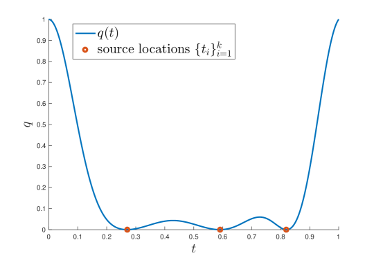
Figure 3: Example of dual certificate $q(t)$ required in Lemma 14. Here, we have $k=3$ and $t_{1}=0.27,t_{2}=0.59$ and $t_{3}=0.82$.

3.2 Stabilising dual polynomials for non-negative sparse measures: proof of Theorem 11

We develop the proof of Theorem 11 by using a dual polynomial analogous to that in Lemma 14, but with further guarantees that away from the sources the dual polynomial must be sufficiently bounded away from the constraint bounds. However, first, let us bring the generality of Theorem 11 to discrete measures by introducing an intermediate measure $\chi$ which is $k$-discrete and whose support is $2\epsilon$ separated. Noting that the measurement operator $\Phi$ is $L$-Lipschitz, see (22), and using the triangle inequality, it follows that

$$\left\|y-\int_{I}\Phi(t)\chi(\operatorname{d\!}t)\right\|_{2} \leq\left\|y-\int_{I}\Phi(t)x(\operatorname{d\!}t)\right\|_{2}+\left\|\int_{I}\Phi(t)(x(\operatorname{d\!}t)-\chi(\operatorname{d\!}t))\right\|_{2}$$

$$\leq\delta+L\cdot d_{GW}\left(x,\chi\right)=\mathrel{\mathop{\mathchar 58\relax}}\delta^{\prime}.$$ (35)

Therefore, a solution $\widehat{x}$ of Program (4) with $\delta^{\prime}$ specified above can be considered as an estimate of $\chi$. In the rest of this section, we first bound the error $d_{GW}(\chi,\widehat{x})$ and then use the triangle inequality to control $d_{GW}(x,\widehat{x})$.

To control $d_{GW}(\chi,\widehat{x})$ in turn, we will first show that the existence of certain dual certificates leads to stability of Program (4). Then we see that these certificates exist under certain conditions on the measurement operator $\Phi$. Turning now to the details, the following result is slightly more general than the one in [40] and guarantees the stability of Program (4) if a prescribed dual certificate $q$ exists. The proof is provided in Appendix B.

Lemma 16.

(Error away from the support) Let $\widehat{x}$ be a solution of Program (4) with $\delta^{\prime}$ specified in (35) and set $h=\widehat{x}-\chi$ to be the error. Consider $F(t)$ given in Definition 10 and suppose that there exist a positive $\epsilon\leq\Delta(T)/2$, real coefficients $\{b_{j}\}_{j=1}^{m}$, and a polynomial $q=\sum_{j=1}^{m}b_{j}\phi_{j}$ such that

$$q(t)\geq F(t),$$

where the equality holds on $T$. Then we have that

$$\bar{f}\int_{T_{\epsilon}^{C}}h(\operatorname{d\!}t)+\sum_{i=1}^{k}\int_{T_{i,\epsilon}}f\left(t-t_{i}\right)h(\operatorname{d\!}t)\leq 2\|b\|_{2}\delta^{\prime},$$ (36)

where $b\in\mathbb{R}^{m}$ is the vector formed by the coefficients $\{b_{j}\}_{j=1}^{m}$.

There is a natural analogy here with the case of exact samples. In the setting where $\eta_{i}=0$ in (2), the dual certificate $q$ in Lemma 14 was required to be positive off the support $T$. In the presence of inexact samples however, Lemma 16 loosely-speaking requires the dual certificate to be bounded away from zero (see example in Figure 4) for $t\in T_{\epsilon}^{C}$.

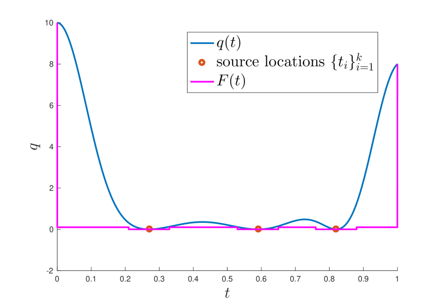
(a)

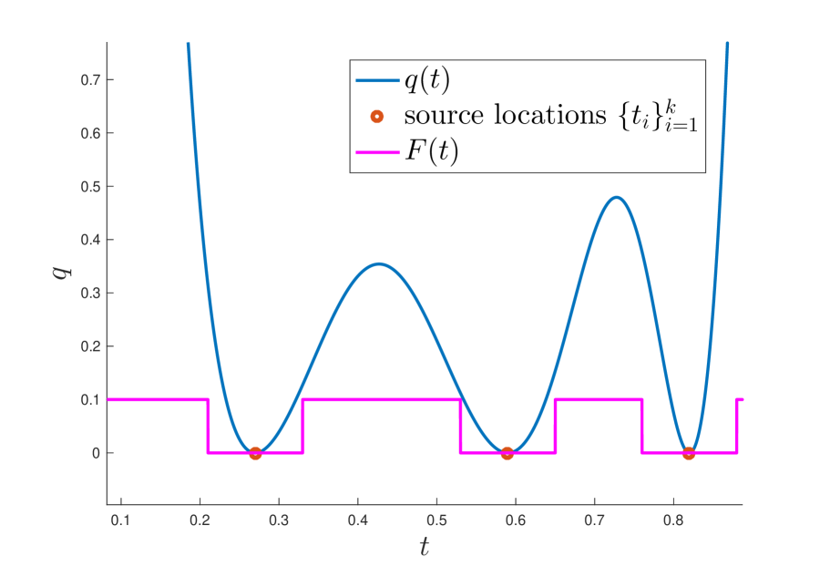
(b)

Figure 4: Example of dual certificate $q(t)$ that satisfies the conditions in Lemma 16 where the window function is the Gaussian kernel $\phi(t)=e^{-t^{2}/\sigma^{2}}$. We take $k=3$ and $t_{i}\in\{0.27,0.59,0.82\}$ and the function $F(t)$ such that $q(t)\geq F(t)$.

Note also that Lemma 16 controls the error $h$ away from the support $T$, as it guarantees that

$$\int_{T_{\epsilon}^{C}}h(\operatorname{d\!}t)\leq\frac{2\|b\|_{2}\delta^{\prime}}{\bar{f}},$$ (37)

if the dual certificate $q$ exists. Indeed, (37) follows directly from (36) because the sum in (36) is non-negative. This is in turn the case because $f(0)=0$ and the error $h$ is non-negative off the support $T$. Another key observation is that Lemma 16 is almost silent about the error near the impulses in $\chi$. Indeed, because $f(0)=0$ by assumption, (36) completely fails to control the error on the support $T$. However, as the next result states, Lemma 16 can be strengthened near the support provided that an additional dual certificate $q^{0}$ exists. The proof, given in Appendix C, is not unsimilar to the analysis in [41].

Lemma 17.

(Error near the support) Suppose that the dual certificate in Lemma 16 exists. Consider a function $F^{0}(t)$ defined like $F^{\pi}(t)$ in Definition 10 for the sign pattern $\pi^{0}$ such that

$$\pi^{0}_{i}=\begin{cases}1,&\text{when there exists }i\in[k]\text{ such that }t\in T_{i,{\epsilon}}\text{ and }\int_{T_{i,{\epsilon}}}h(\operatorname{d\!}t)>0,\\ -1,&\text{when there exists }i\in[k]\text{ such that }t\in T_{i,{\epsilon}}\text{ and }\int_{T_{i,{\epsilon}}}h(\operatorname{d\!}t)\leq 0,\end{cases}$$

and suppose also that there exist real coefficients $\{b_{j}^{0}\}_{j\in[m]}$ and a polynomial $q^{0}=\sum_{j=1}^{m}b_{j}^{0}\phi_{j}$ such that

$$q^{0}(t)\geq F^{0}(t),$$

where the equality holds on $T$. Then we have that

$$\sum_{i=1}^{k}\left|\int_{T_{i,{\epsilon}}}h(\operatorname{d\!}t)\right|\leq 2\left(\|b\|_{2}+\|b^{0}\|_{2}\right)\delta^{\prime}.$$ (38)

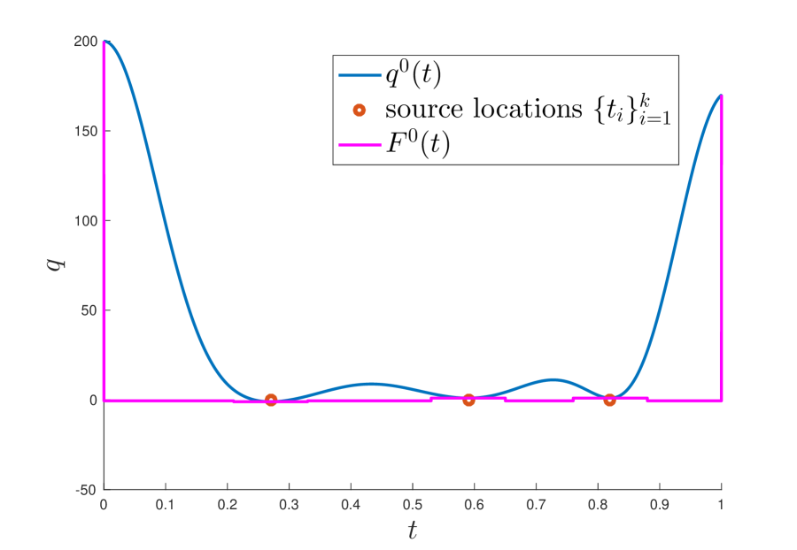
(a)

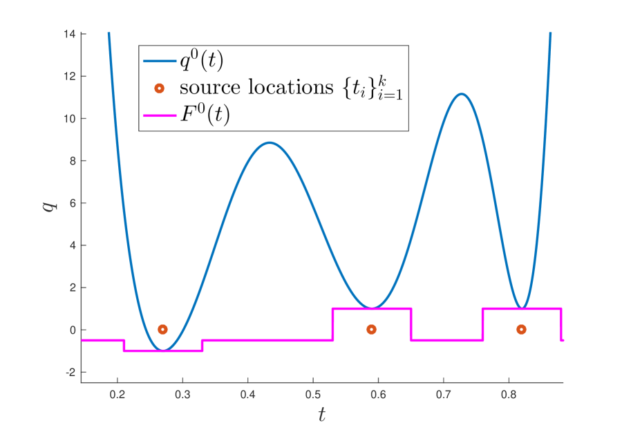
(b)

Figure 5: Example of dual certificate $q^{0}(t)$ that satisfies the conditions in Lemma 17 where the window function is the Gaussian kernel $\phi(t)=e^{-t^{2}/\sigma^{2}}$. We take $k=3$ and $t_{i}\in\{0.27,0.59,0.82\}$ and the function $F^{0}(t)$ for the sign pattern $\pi^{0}=\{-1,1,1\}$ such that $q^{0}(t)\geq F^{0}(t)$. For the Gaussian kernel, the existence of $q^{\pi}(t)$ for any sign pattern $\pi$ guarantees the existence of $q^{0}(t)$ in Lemma 17.

In words, Lemma 17 controls the error $h$ near the support $T$, provided that a certain dual certificate $q^{0}$ exists (see example in Figure 5). Note that (38) does not control the mass of the error, namely $\sum_{i}\int_{T_{i,\epsilon}}|h(\operatorname{d\!}t)|=\int_{T_{\epsilon}}|h(\operatorname{d\!}t)|$, but rather it controls $\sum_{i}|\int_{T_{i,\epsilon}}h(\operatorname{d\!}t)|$. Of course, the latter is always bounded by the former, that is

$$\sum_{i=1}^{k}\left|\int_{T_{i,{\epsilon}}}h(\operatorname{d\!}t)\right|\leq\int_{T_{{\epsilon}}}|h(\operatorname{d\!}t)|.$$ (39)

However, the two sides of (39) might differ significantly. For instance, it might happen that the solution $\widehat{x}$ returns a slightly incorrect impulse at $t_{i}+\epsilon/4$ (rather than $t_{i}$) but with the correct amplitude of $a_{i}$. As a result, the mass of the error is large in this case ($\int_{T_{i,\epsilon}}|h(\operatorname{d\!}t)|=2a_{i}$) but the left-hand side of (39) vanishes, namely $|\int_{T_{i,\epsilon}}h(\operatorname{d\!}t)|=0$. Note that we cannot hope to strengthen (38) by replacing its left-hand side with the mass of the error, namely $\int_{T_{\epsilon}}|h(\operatorname{d\!}t)|$. This is the case mainly because the total variation is not the appropriate error metric for this context.

Indeed, while the mass of the error $\int_{I}|h(\operatorname{d\!}t)|$ might not be small in general, we can instead control the generalised Wasserstein distance between the true and estimated measures, namely $x$ and $\widehat{x}$, see (19) and (20). The following result is proved by combining Lemmas 16 and 17, see Appendix D.

Lemma 18.

(Stability of Program (4) in the Generalised Wasserstein distance) Suppose that the dual certificates in Lemmas 16 and 17 exist. Then it holds that

$$d_{GW}\left(\chi,\widehat{x}\right)\leq\left(\left(6+\frac{2}{\bar{f}}\right)\|b\|_{2}+6\|b^{0}\|_{2}\right)\delta^{\prime}+\epsilon\|\chi\|_{TV}.$$ (40)

An application of triangle inequality now yields that

$$d_{GW}(x,\widehat{x}) \leq d_{GW}(x,\chi)+d_{GW}(\chi,\widehat{x})$$

$$\leq d_{GW}(x,\chi)+\left(\left(6+\frac{2}{\bar{f}}\right)\|b\|_{2}+6\|b^{0}\|_{2}\right)\delta^{\prime}+\epsilon\|\chi\|_{TV}.\qquad\mbox{(see Lemma \ref{lem:EMD})}$$ (41)

In words, Program (4) is stable $x$ if the certificates $q$ and $q^{0}$ exist. Let us now study the existence of these certificates. Proposition 19, proved in Appendix E, guarantees the existence of the dual certificate $q$ required in Lemma 16 and heavily relies on the concept of T*-system in Definition 9. We remark that the proof benefits from the ideas in [27]. Similarly, Proposition 20, stated without proof, ensures the existence of the certificate $q^{0}$ required in Lemma 17.

Proposition 19.

(Existence of $q$) For $m\geq 2k+2$, suppose that $\{\phi_{j}\}_{j=1}^{m}$ form a T-system on $I$ and that $\{F\}\cup\{\phi_{j}\}_{j=1}^{m}$ form a T*-system on $I$, where $F(t)$ is the function given in Definition 10. Then the dual certificate $q$ in Lemma 16 exists and consequently Program (4) is stable in the sense that (36) holds.

Note that to ensure the success of Program (4), it suffices that there exists a polynomial $q=\sum_{j=1}^{m}b_{j}\phi_{j}$ such that $q(t)\geq F(t)$ with the equality met on the support $T$, see Lemma 16. Equivalently, it suffices that there exists a non-negative polynomial $\dot{q}=-b_{0}F+\sum_{j=1}^{m}b_{j}\phi_{j}$ that vanishes on $T$ such that $b_{0}>0$ and at least one other coefficient, say $b_{j_{0}}$, is nonzero. This situation is reminiscent of Lemma 15. In contrast to Lemma 15, however, such $\dot{q}$ exists when $\{F\}\cup\{\phi_{j}\}_{j=1}^{m}$ is a T*-system rather than a T-system. The more subtle T*-system requirement is to avoid trivial or unbounded polynomials.

Proposition 20.

(Existence of $q^{0}$) For $m\geq 2k+2$, suppose that $\{\phi_{j}\}_{j=1}^{m}$ form a T-system on $I$ and that $\{F^{0}\}\cup\{\phi_{j}\}_{j=1}^{m}$ form a T*-system on $I$, where $F^{0}(t)$ is the function defined in Lemma 17. Then the dual certificate $q^{0}$ in Lemma 17 exists and consequently Program (4) is stable in the sense that (38) holds.

Having constructed the necessary dual certificates in Propositions 19 and 20, the proof of Theorem 11 is now complete in light of (41).

3.3 Proof of Theorem 12 (Average stability for Program (4))

In this section we give an overview of the main ideas involved in proving Theorem 12. To start with, let $A\in\mathbb{R}^{k\times k}$ be defined as in (30):

$$A=\begin{bmatrix}|\phi_{1}(t_{1})|&-|\phi_{1}(t_{2})|&\ldots&-|\phi_{1}(t_{k})|\\ -|\phi_{2}(t_{1})|&|\phi_{2}(t_{2})|&\ldots&-|\phi_{2}(t_{k})|\\ \vdots&\vdots&\ddots&\vdots\\ -|\phi_{k}(t_{1})|&-|\phi_{k}(t_{2})|&\ldots&|\phi_{k}(t_{k})|\\ \end{bmatrix},$$

where $\phi_{i}(t_{i})=\phi(t_{i}-s_{l(i)})$ is evaluated at the source $t_{i}$ and the closest sample to it, as defined in (7).

The proof of Theorem 12 consists of two steps. We first show that we can bound the error if the matrix $A$ is strictly diagonally dominant. It is easy to see that, if the window function $\phi$ is localised, then the entries on the main diagonal are larger in absolute value than the off-diagonal entries. If, moreover, we choose the sampling locations $\{s_{i}\}_{i\in[m]}$ such that $A$ is strictly diagonally dominant (which means that for each source, there is a sampling location that is "close enough" to it), then the bound (28) is guaranteed.

Proposition 21.

For each source $t_{i}$, select $s_{l(i)}$ to be the closest sample as defined in (7), and define the matrix A in (30) using the sequences $\{t_{i}\}_{i=1}^{k}$, $\{s_{l(i)}\}_{i=1}^{k}$. If $A$ is strictly diagonally dominant, then the error around the support is bounded according to (28).

Then, we want to go further and see what it means exactly for $A$ to be strictly diagonally dominant, so the second step in the proof of Theorem 12 is to give an upper bound for the distance between the sources $\{t_{i}\}_{i\in[k]}$ and the closest sampling locations $\{s_{l(i)}\}_{i\in[k]}$ such that $A$ is strictly diagonally dominant.

Given an even positive function $\phi$ that is localised at $0$ and with fast decay, let $\Delta$ and $\lambda$ as given in Definition 1, so

$$|t_{i}-s_{l(i)}|\leq\lambda\Delta$$ (42)

We want to find $\lambda_{0}$ such that

$$\phi(s_{l(i)}-t_{i})\geq\sum_{j\neq i}\phi(s_{l(i)}-t_{j}),\quad\forall\lambda\in(0,\lambda_{0}),\quad\forall i\in[k],$$ (43)

namely, we want the matrix $A$ to be strictly diagonally dominant. From the conditions (43), we can obtain a more general equality, depending on $\phi$ and $\Delta$, that $\lambda_{0}$ must satisfy such that, for $\lambda<\lambda_{0}$, $A$ is strictly diagonally dominant. The equality is given by (27):

$$\phi(\lambda_{0}\Delta)=\phi(\Delta-\lambda_{0}\Delta)+\phi(\Delta+\lambda_{0}\Delta)+\frac{1}{\Delta}\int_{\Delta-\lambda_{0}\Delta}^{1/2-\lambda_{0}\Delta}\phi(x)\operatorname{d\!}x+\frac{1}{\Delta}\int_{\Delta+\lambda_{0}\Delta}^{1/2+\lambda_{0}\Delta}\phi(x)\operatorname{d\!}x.$$

Proposition 22.

Let $\lambda_{0}\in(0,\frac{1}{2})$ such that $\left|t_{i}-s_{l(i)}\right|\leq\lambda_{0}\Delta$ for all $i\in[k]$. If $\lambda_{0}$ satisfies (27), then the matrix A defined in (30) is strictly diagonally dominant.

Finally, we note that the proof of Theorem 13 involves the same ideas as the ones discussed in this section, with a few modifications. The detailed proofs of Proposition 21 and Proposition 22 are given in Appendices F and G respectively. The proof of Theorem 13 is similar to the proof presented in the current section, so we only show the differences in Appendix H.

3.4 Proofs of Theorems 4 and 5 (Gaussian with sparse measure)

In this section we give the main steps taken to obtain the explicit bounds in Theorems 4 and 5 for the Gaussian window function. These are particular cases of the more general Theorems 11 and 12 respectively, where the window function is taken to be the Gaussian $\phi_{j}(t)=e^{-(t-s_{j})^{2}/\sigma^{2}}$, given in (9), and the true measure $x$ is a k-discrete non-negative measure as in (1).

3.4.1 Bounds on the coefficients of the dual certificates for Gaussian window

We will now give explicit bounds on the vectors of coefficients $\|b\|_{2}$ and $\|b^{\pi}\|_{2}$ of the dual certificates $q$ and $q^{\pi}$ from Lemmas 16 and 17 in terms of the parameters of the problem $k,T,S$ and $\sigma$ (the width of the Gaussian window).

Firstly, we introduce a more specific form of the dual polynomial separators $F(t)$, $F^{\pi}(t)$ from Definition 10. Here, we take $f(t)=0$ for $t\in(-\epsilon,\epsilon)$ and $\bar{f},f_{1}$ positive constants with $\bar{f}<1$. Then, $f_{0}$ is defined to be greater that both $\bar{f}$ and $f_{1}$, with the exact relationship between $f_{0}$ and $\bar{f}$ given in the proof of Lemma 23. Therefore, for $\epsilon>0$ and a sign pattern $\pi\in\{\pm 1\}^{k}$, $F(t)$ and $F^{\pi}(t)$ are:

$$F(t) =\begin{cases}{f}_{0},&t=0,\\ {f}_{1},&t=1,\\ 0,&\text{when there exists }i\in[k]\text{ such that }t\in{T}_{i,{\epsilon}},\\ \bar{f},&\text{elsewhere on }I.\end{cases}$$ (44)

$$F^{\pi}(t) =\begin{cases}f_{0},&t=0,\\ f_{1},&t=1,\\ \pi_{i},&\text{when there exists }i\in[k]\text{ such that }t\in{T}_{i,\epsilon},\\ -\bar{f},&\mbox{elsewhere on }I.\end{cases}$$ (45)

With the above definitions, both Theorem 11 and Theorem 12 require that $\{F\}\cup\{\phi_{j}\}_{j=1}^{m}$ form a T*-system on $I$. Likewise, Theorem 11 requires that $\{F^{\pi}\}\cup\{\phi_{j}\}_{j=1}^{m}$ form a T*-system for any sign pattern $\pi$. We show in Lemma 23 that both these requirements are satisfied for the choice in (9) of $\phi_{j}(t)=e^{-(t-s_{j})^{2}/\sigma^{2}}$. The proof is given in Appendix J.

Lemma 23.

Consider the function $F(t)$ defined in (44) and suppose that $m\geq 2k+2$. Then $\{F\}\cup\{\phi_{j}\}_{j=1}^{m}$ form a T*-system on $I$, with $\phi$ extended totally positive, even Gaussian and $\phi_{j}$ defined as in (9), provided that $f_{0}\gg\bar{f}$, $f_{0}\gg f_{1}$ and $\bar{f},f_{0},f_{1}\gg 0$. These requirements are made precise in the proof and are dependent on $\epsilon$. Moreover, for an arbitrary sign pattern $\pi$ and $F^{\pi}$ as defined in (45), $\{F^{\pi}\}\cup\{\phi_{j}\}_{j=1}^{m}$ form a T*-system on $I$ when, in addition, $f_{0}\gg 1$.

In this setting, consider a subset of $m=2k+2$ samples $\{s_{j}\}_{j=1}^{m}\subset S$ (since in the proof of Lemma 23 we select the $2k+2$ samples that are the closest to the sources) such that they satisfy Conditions 2. Therefore, we have that $s_{1}=0$, $s_{m}=s_{2k+2}=1$, and

$$|s_{2i}-t_{i}|\leq\eta,\qquad s_{2i+1}-s_{2i}=\eta,\qquad\forall i\in[k],$$ (46)

for a small $\eta\leq\sigma^{2}$, see (9). That is, we collect two samples close to each impulse $t_{i}$ in $x$, one on each side of $t_{i}$.

Suppose also that

$$\sigma\leq\sqrt{2},\quad\Delta>\sigma\sqrt{\log\left(3+\frac{4}{\sigma^{2}}\right)},\quad\eta\leq\sigma^{2},$$ (47)

namely the width of the Gaussian is much smaller than the separation of the impulses in $x$. Lastly, assume that the impulse locations $T=\{t_{i}\}_{i=1}^{k}$ and sampling points $\{s_{j}\}_{j=2}^{m-1}$ are away from the boundary of $I$, namely

$$\sigma\sqrt{\log(1/\eta^{3})}\leq t_{i}\leq 1-\sigma\sqrt{\log(1/\eta^{3})},\qquad\forall i\in[k],$$

$$\sigma\sqrt{\log(1/\eta^{3})}\leq s_{j}\leq 1-\sigma\sqrt{\log(1/\eta^{3})},\qquad\forall j\in[2\mathrel{\mathop{\mathchar 58\relax}}m-1].$$ (48)

Remark 1. The Property 2. Samples near sources in Conditions 2 states that for each two samples $s^{\prime}$ and $s$ near each source, we have that:

$$C_{1}\eta\leq s^{\prime}-s\leq C_{2}\eta,$$ (49)

but in (46) above we simplified the condition to $s_{2i+1}-s_{2i}=\eta$. Throughout the proofs in this paper we will use the simplified condition in (46) instead of the more general (49) so that we do not obscure the central issues of the proof with extra indices and separate treatment of the upper and lower bounds for $s^{\prime}-s$. This has implications for Lemma 24 below, and we will point out the places in its proof where using the more general condition (49) would require separate treatment (see footnotes 6 and 8).

Remark 2. The Property 3. Sources away from the boundary in Conditions 2 is necessary due to our method of proof, which imposes that the sources and samples are in the interval $I=[0,1]$ independently from the width $\sigma$ of the convolution kernel and the minimum separation of sources $\Delta$. While the exact form of the boundary conditions depend on the specific approach that we took in the proof, there is an interplay between $\sigma$ and $\Delta$ in the noisy setting and due to the fact that the interval $I=[0,1]$ is fixed, some form of scaling is required, which is what this condition achieves. For example, for $\sigma=1$, the Gaussian kernel defined in (10) varies by at most $\frac{1}{e}$ (between two sources located at $t_{1}=0$ and $t_{2}=1$) and therefore our results for the noisy setting are not meaningful for large $\sigma$.

We can now give explicit bounds on $\|b\|_{2}$ and $\|b^{\pi}\|_{2}$ for the Gaussian window function, as required by Theorems 11 and 12. The following result is proved in Appendix K.

Lemma 24.

Suppose that the window function $\phi$ is Gaussian, as defined in (9), the assumptions (46), (47) and (48) (namely Conditions 2) hold and $\eta$ satisfies:

$$\eta\leq\min\left\{\frac{8F_{\min}(\Delta,\frac{1}{\sigma})}{34(2k+2)\left(80k+8+kP\left(\frac{1}{\sigma}\right)\frac{2}{1-e^{-\frac{\Delta^{2}}{\sigma^{2}}}}\right)^{\frac{1}{2}}},\frac{\bar{C}(f_{0},f_{1})^{\frac{1}{6}}}{\left(4k+4+\frac{4k}{\sigma^{2}}\right)^{\frac{1}{3}}}\right\}.$$ (50)

Then we have the following bounds:

$$\|b\|_{2} \leq\frac{\sqrt{(2k+2)\left(4k+5+\frac{4k}{\sigma^{4}}\right)}}{1-\frac{\sqrt{e}}{2}}\bar{C}(f_{0},f_{1})^{\frac{5}{4}}\left[\frac{F_{\max}\left(\Delta,\frac{1}{\sigma}\right)}{F_{\min}\left(\Delta,\frac{1}{\sigma}\right)^{2}}\right]^{k},$$ (51)

$$\|b^{\pi}\|_{2} \leq\frac{\sqrt{2k+2}}{\eta\left(1-\frac{\sqrt{e}}{2}\right)}\left(\bar{C}(f_{0},f_{1})+2k\right)^{\frac{3}{2}}\left[\frac{F_{\max}\left(\Delta,\frac{1}{\sigma}\right)}{F_{\min}\left(\Delta,\frac{1}{\sigma}\right)^{2}}\right]^{k},$$ (52)

where

$$\bar{C}(f_{0},f_{1})=f_{0}^{2}+f_{1}^{2}+2f_{0}+2f_{1}+2,$$ (53)

$$P\left(\frac{1}{\sigma}\right)=\frac{4}{\sigma^{4}}+\frac{13}{4}\left(\frac{2}{\sigma^{2}}+\frac{4}{\sigma^{4}}\right)^{2}+\frac{9}{4}\left(\frac{12}{\sigma^{4}}+\frac{8}{\sigma^{6}}\right)^{2}.$$ (54)

$$F_{\max}\left(\Delta,\frac{1}{\sigma}\right)=\left(8+\left(1+\frac{4}{\sigma^{4}}\right)\frac{2}{1-e^{-\frac{\Delta^{2}}{\sigma^{2}}}}\right)^{\frac{1}{2}}\left(32+\left(\frac{1}{\sigma^{4}}+\frac{2}{\sigma^{6}}+\frac{2}{\sigma^{8}}\right)\frac{16}{1-e^{-\frac{\Delta^{2}}{\sigma^{2}}}}\right)^{\frac{1}{2}},$$ (55)

$$F_{\min}\left(\Delta,\frac{1}{\sigma}\right)=1-\left(1+\frac{2}{\sigma^{2}}\right)\frac{2e^{-\frac{\Delta^{2}}{\sigma^{2}}}}{1-e^{-\frac{\Delta^{2}}{\sigma^{2}}}}.$$ (56)

To obtain the final bounds for the Gaussian window function, we will substitute the above bounds in the right hand side of (26) in Theorem 11 and in (28) and (29) in Theorem 12. We will then obtain $F_{1}$ in Theorem 4 (see (65)) and $F_{2}$ in Theorem 5 (see (72)).

For more clarity, in the following lemma we simplify $F_{1}$ and $F_{2}$ further, in the case when stronger conditions apply to $\sigma$, $\Delta(T)$ and $\lambda$.

Lemma 25.

If the conditions in Lemma 24 hold and, in addition, $\sigma<\frac{1}{\sqrt{3}}$, $\Delta>\sigma\sqrt{\log{\frac{5}{\sigma^{2}}}}$ and $\bar{f}<1$, then

$$\frac{F_{\max}\left(\Delta,\frac{1}{\sigma}\right)}{F_{\min}\left(\Delta,\frac{1}{\sigma}\right)^{2}}<\frac{c_{1}}{\sigma^{6}(1-3\sigma^{2})^{2}},$$ (57)

$$\left((6+\frac{2}{\bar{f}})\sqrt{4k+5+\frac{4k}{\sigma^{4}}}\bar{C}(f_{0},f_{1})^{\frac{5}{4}}+\frac{6}{\eta}(\bar{C}(f_{0},f_{1})+2k)^{\frac{3}{2}}\right)\frac{\sqrt{2k+2}}{1-\frac{\sqrt{e}}{2}}<c_{2}\cdot\frac{kC_{1}(\frac{1}{\epsilon})}{\eta\sigma^{2}},$$ (58)

$$\frac{\sqrt{(2k+2)\left(4k+5+\frac{4k}{\sigma^{4}}\right)}}{1-\frac{\sqrt{e}}{2}}\frac{\bar{C}(f_{0},f_{1})^{\frac{5}{4}}}{\bar{f}}<c_{3}\cdot\frac{kC_{2}(\frac{1}{\epsilon})}{\sigma^{2}},$$ (59)

where

$$C_{1}\left(\frac{1}{\epsilon}\right) =\frac{(\bar{C}(f_{0},f_{1})+2k)^{\frac{3}{2}}}{\bar{f}},$$ (60)

$$C_{2}\left(\frac{1}{\epsilon}\right) =\frac{\bar{C}(f_{0},f_{1})^{\frac{5}{4}}}{\bar{f}},$$ (61)

and, similarly, the condition (50) is simplified to condition (13). Moreover, if $\lambda$ in Theorem 12 satisfies $\lambda<\frac{2}{4}$, then

$$\frac{1}{e^{-\frac{\Delta^{2}\lambda^{2}}{\sigma^{2}}}-e^{-\frac{\Delta^{2}\lambda^{2}}{\sigma^{2}}}\cdot\frac{e^{-\frac{\Delta^{2}}{\sigma^{2}}}+e^{-\frac{2\Delta^{2}}{\sigma^{2}}}}{1-e^{-\frac{\Delta^{2}}{\sigma^{2}}}}-e^{-\frac{\Delta^{2}(1-\lambda)^{2}}{\sigma^{2}}}}<c_{4}.$$ (62)

Above, $c_{1},c_{2},c_{3},c_{4}$ are universal constants.

More specifically, (57), (58) will be used to bound $F_{1}$ to obtain (12) and (57), (59), will be used to bound $F_{2}$ to obtain (16). Lastly, (62) will be used to bound $F_{3}$, which appears in the bound given by Theorem 5.

The proof of Lemma 25 is given in Appendix N. Note that we give $C_{1}$ and $C_{2}$ as functions of $\frac{1}{\epsilon}$ because, as $\epsilon\to 0$, $C_{1}$ and $C_{2}$ grow at a rate dependent on $\epsilon$, as indicated in the Lemma 27 in Section 3.4.4.

3.4.2 Proof of Theorem 4 (Wasserstein stability of Program (4) for $\phi(t)$ Gaussian)

We consider Theorem 11 and restrict ourselves to the case $x=\chi$, a k-discrete non-negative measure as in (1) with support $T$. Let $\Delta=\Delta(T)\geq 2\epsilon$, with $T$ as the support of $x$. We begin with estimating the Lipschitz constant of the measurement operator $\Phi$ according to (22), see Appendix I for the proof of the next result.

Lemma 26.

Consider $S=\{s_{j}\}_{j=1}^{m}\subset\mathbb{R}$ and $\{\phi_{j}\}_{j=1}^{m}$ specified in (9). Then the operator $\Phi\mathrel{\mathop{\mathchar 58\relax}}I\rightarrow\mathbb{R}^{m}$ defined in (3) is $\frac{2\sqrt{m}}{\sigma\sqrt{2e}}$-Lipschitz with respect to the generalised Wasserstein distance, namely (22) holds with $L=\frac{2\sqrt{m}}{\sigma\sqrt{2e}}$.

We may now invoke Theorem 11 to conclude that, for an arbitrary $k$-sparse $2\epsilon$-separated non-negative measure $x$ and arbitrary sampling points $\{s_{j}\}_{j=1}^{m}\subset\mathbb{R}$, Program (4) with $\delta^{\prime}=\delta$ is stable in the sense that there exist vectors $b,\{b^{\pi}\}_{\pi}\subset\mathbb{R}^{m}$ such that

$$d_{GW}\left(x,\widehat{x}\right)\leq\left(\left(6+\frac{2}{\bar{f}}\right)\|b\|_{2}+6\min_{\pi}\|b^{\pi}\|_{2}\right)\cdot\delta+\|x\|_{TV}\cdot\epsilon$$ (63)

provided that $m\geq 2k+2$ and $f_{0}\gg f_{1}\gg\bar{f}\gg 0$. The exact relationships between $\bar{f},f_{0},f_{1}$ are given in the proof of Lemma 23 in Appendix J.

Combining Lemma 24 with (63) yields a final bound on the stability of Program (4) with Gaussian window and completes the proof of the first part of Theorem 4:

$$d_{GW}(x,\widehat{x})\leq F_{1}(k,\Delta(T),\frac{1}{\sigma},\frac{1}{\epsilon},\eta)\cdot\delta+\|x\|_{TV}\cdot\epsilon,$$ (64)

where

$$F_{1}(k,\Delta(T),\frac{1}{\sigma},\frac{1}{\epsilon},\eta)=\left((6+\frac{2}{\bar{f}})\sqrt{4k+5+\frac{4k}{\sigma^{4}}}\bar{C}^{\frac{5}{4}}+\frac{6}{\eta}(\bar{C}+2k)^{\frac{3}{2}}\right)\frac{\sqrt{2k+2}}{1-\frac{\sqrt{e}}{2}}\left(\frac{F_{\max}\left(\Delta,\frac{1}{\sigma}\right)}{F_{\min}\left(\Delta,\frac{1}{\sigma}\right)^{2}}\right)^{k},$$ (65)

with $\bar{C},F_{\max},F_{\min}$ given in (53), (55), (56) respectively and $f_{0}=f_{0}(\frac{1}{\epsilon})$ depends on $\epsilon$ (see the proof of Lemma 27).

Finally, to show that (12) holds when $\sigma<\frac{1}{\sqrt{3}}$, and $\Delta>\sigma\sqrt{\log{\frac{5}{\sigma^{2}}}}$, we apply the first part of Lemma 25 with $\bar{f}<1$ and the proof of Theorem 4 is complete.

Remark. In particular, $f_{0}$ increases as $\epsilon\to 0$ and $f_{0}$ also depends on the other parameters of the problem, namely $\eta,\sigma,\Delta(T),k$. See Section 3.5 for a detailed discussion. Furthermore, $f_{1}$ and $\bar{f}$ are considered fixed positive constants with $f_{1}<f_{0}$.

3.4.3 Proof of Theorem 5 (Average stability of Program (4) for $\phi(t)$ Gaussian: source proximity dependence)

We now apply Theorem 12 with $\phi(t)=g(t)=e^{-t^{2}/\sigma^{2}}$. We have that $\phi^{\infty}=1$, the Lipschitz constant $L$ of $g$ on $[-1,1]$ is $L=\frac{2}{\sigma^{2}}$, and

$$\sum_{j=1}^{k}(A^{-1})_{ij}\leq\|A^{-1}\|_{\infty}<\frac{1}{\min_{j}\left(g(s_{j}-t_{j})-\sum_{i\neq j}g(s_{j}-t_{i})\right)}.$$ (66)

The last inequality comes from the definition of $A$ in (30) with $\phi(t)=g(t)$ and $s_{j}\mathrel{\mathop{\mathchar 58\relax}}=s_{l(j)}$ as given in Definition 1, and [42]. Then, by assumption, $|s_{j}-t_{j}|\leq\lambda\Delta$ for an arbitrary $j\in[k]$ and $g$ is decreasing, so

$$g(s_{j}-t_{j})\geq g(\lambda\Delta)=e^{-\frac{\lambda^{2}\Delta^{2}}{\sigma^{2}}}.$$

We now assume without loss of generality that $s_{j}<t_{j}$. Then, it follows that

$$|s_{j}-t_{i}|\geq|j-i|\Delta-\lambda\Delta,\text{ if }i<j\quad\quad\text{ and }\quad\quad|s_{j}-t_{i}|\geq|j-i|\Delta+\lambda\Delta,\text{ if }i>j.$$

This, in turn, leads to

$$\sum_{i\neq j}g(s_{j}-t_{i}) =\sum_{i=1}^{j-1}g(s_{j}-t_{i})+\sum_{i=j+1}^{k}g(s_{j}-t_{i})$$

$$\leq\sum_{i=1}^{j-1}g((j-i)\Delta-\lambda\Delta)+\sum_{i=j+1}^{k}g((i-j)\Delta+\lambda\Delta)$$

$$\leq\sum_{i=1}^{\infty}g((i-\lambda)\Delta)+\sum_{i=1}^{\infty}g((i+\lambda)\Delta).$$ (67)

We now bound each sum in (67) as follows

$$\sum_{i=1}^{\infty}g((i-\lambda)\Delta) =\sum_{i=1}^{\infty}e^{-\frac{(i-\lambda)^{2}\Delta^{2}}{\sigma^{2}}}$$

$$=e^{-\frac{\Delta^{2}(1-\lambda)^{2}}{\sigma^{2}}}+e^{-\frac{\Delta^{2}\lambda^{2}}{\sigma^{2}}}\sum_{i=2}^{\infty}\left(e^{-\frac{\Delta^{2}}{\sigma^{2}}}\right)^{i^{2}-2i\lambda}$$

$$\leq e^{-\frac{\Delta^{2}(1-\lambda)^{2}}{\sigma^{2}}}+e^{-\frac{\Delta^{2}\lambda^{2}}{\sigma^{2}}}\sum_{i=2}^{\infty}\left(e^{-\frac{\Delta^{2}}{\sigma^{2}}}\right)^{i}\quad\quad\quad(i^{2}-2i\lambda>i\text{ for }i\geq 2)$$

$$=e^{-\frac{\Delta^{2}(1-\lambda)^{2}}{\sigma^{2}}}+e^{-\frac{\Delta^{2}\lambda^{2}}{\sigma^{2}}}\cdot\frac{e^{-\frac{2\Delta^{2}}{\sigma^{2}}}}{1-e^{-\frac{\Delta^{2}}{\sigma^{2}}}},$$ (68)

and similarly, we have that

$$\sum_{i=1}^{\infty}g((i+\lambda)\Delta)=\sum_{i=1}^{\infty}e^{-\frac{(i+\lambda)^{2}\Delta^{2}}{\sigma^{2}}}\leq e^{-\frac{\Delta^{2}\lambda^{2}}{\sigma^{2}}}\cdot\frac{e^{-\frac{\Delta^{2}}{\sigma^{2}}}}{1-e^{-\frac{\Delta^{2}}{\sigma^{2}}}}.$$ (69)

By combining (67), (68) and (69), we obtain:

$$g(s_{j}-t_{j})-\sum_{i\neq j}g(s_{j}-t_{i})\geq e^{-\frac{\Delta^{2}\lambda^{2}}{\sigma^{2}}}-e^{-\frac{\Delta^{2}\lambda^{2}}{\sigma^{2}}}\cdot\frac{e^{-\frac{\Delta^{2}}{\sigma^{2}}}+e^{-\frac{2\Delta^{2}}{\sigma^{2}}}}{1-e^{-\frac{\Delta^{2}}{\sigma^{2}}}}-e^{-\frac{\Delta^{2}(1-\lambda)^{2}}{\sigma^{2}}}.$$ (70)

The above inequality also holds when we take the minimum over $j\in[k]$ and, inserting it in (66) and using this result and the bound on $\|b\|_{2}$ from Lemma 24 in (28), we obtain (14):

$$\left|\int_{T_{i,\epsilon}}\hat{x}(\operatorname{d\!}t)-a_{i}\right|\leq\left[(c_{1}+F_{2})\cdot\delta+c_{2}\frac{\|\hat{x}\|_{TV}}{\sigma^{2}}\cdot\epsilon\right]F_{3},$$ (71)

where

$$F_{2}(k,\Delta(T),\frac{1}{\sigma},\frac{1}{\epsilon})=\frac{\sqrt{(2k+2)\left(4k+5+\frac{4k}{\sigma^{4}}\right)}}{1-\frac{\sqrt{e}}{2}}\frac{\bar{C}(f_{0},f_{1})^{\frac{5}{4}}}{\bar{f}}\left[\frac{F_{\max}\left(\Delta,\frac{1}{\sigma}\right)}{F_{\min}\left(\Delta,\frac{1}{\sigma}\right)^{2}}\right]^{k},$$ (72)

$$F_{3}(\Delta(T),\sigma,\lambda)=\frac{1}{e^{-\frac{\Delta^{2}\lambda^{2}}{\sigma^{2}}}-e^{-\frac{\Delta^{2}\lambda^{2}}{\sigma^{2}}}\cdot\frac{e^{-\frac{\Delta^{2}}{\sigma^{2}}}+e^{-\frac{2\Delta^{2}}{\sigma^{2}}}}{1-e^{-\frac{\Delta^{2}}{\sigma^{2}}}}-e^{-\frac{\Delta^{2}(1-\lambda)^{2}}{\sigma^{2}}}},$$ (73)

and $\bar{C},F_{\max},F_{\min}$ are given in (53), (55), (56) respectively. The error bound away from the sources (15) is obtained by applying Lemma 16 with the same bounds on $\|b\|_{2}$.

Then, by using Lemma 25 with $\bar{f}<1$, we obtain (16). Note that we can apply Lemma 25 because, for $\sigma<\frac{1}{\sqrt{3}}$, we have that $\frac{5}{\sigma^{2}}>3+\frac{4}{\sigma^{2}}$ and, therefore, $\Delta>\sigma\sqrt{\log{\frac{5}{\sigma^{2}}}}>\sigma\sqrt{\log{(3+\frac{4}{\sigma^{2}})}}$.

3.4.4 Proof of Corollary 6

First we give an explicit dependence of $C_{1}(\frac{1}{\epsilon})$ and $C_{2}(\frac{1}{\epsilon})$ on $\epsilon$ for small $\epsilon>0$ in the following lemma, proved in Appendix O.

Lemma 27.

If $f_{1}<f_{0}$, $1<f_{0}$ and $\bar{f}<1$, then there exists $\epsilon_{0}>0$ such that:

$$C_{1}\left(\frac{1}{\epsilon}\right) <\frac{(\bar{c}_{1}C_{\epsilon}^{2}+2k\epsilon^{4})^{\frac{3}{2}}}{\bar{f}}\cdot\frac{1}{\epsilon^{6}}$$ (74)

$$C_{2}\left(\frac{1}{\epsilon}\right) <\bar{c}_{2}C_{\epsilon}^{\frac{5}{2}}\cdot\frac{1}{\epsilon^{5}},$$ (75)

for all $\epsilon\in(0,\epsilon_{0})$, where $\bar{c}_{1}$ and $\bar{c}_{2}$ are universal constants and $C_{\epsilon}$ is defined in the proof, see (295).

To prove the first part of the corollary, we first let $\epsilon=\delta^{\frac{1}{7}}$ in the bound on $C_{1}(\frac{1}{\epsilon})$ in Lemma 27:

$$C_{1}\left(\frac{1}{\epsilon}\right)<\frac{(\bar{c}_{1}C_{\epsilon}^{2}+2k\epsilon^{4})^{\frac{3}{2}}}{\bar{f}}\cdot\frac{1}{\delta^{\frac{6}{7}}},\quad\forall\delta<\epsilon_{0}^{7},$$ (76)

and we substitute the above inequality in the bound (12) in Theorem 4 to obtain:

$$d_{GW}(x,\hat{x})<\bar{C}_{1}\cdot\delta^{\frac{1}{7}},\quad\forall\delta<\epsilon_{0}^{7},$$

where

$$\bar{C}_{1}=\frac{c_{1}k(\bar{c}_{1}C_{\epsilon}^{2}+2k\epsilon^{4})^{\frac{3}{2}}}{\eta\sigma^{2}\bar{f}}\left[\frac{c_{2}}{\sigma^{6}(1-3\sigma^{2})^{2}}\right]^{k}+\|x\|_{TV}.$$ (77)

Similarly, let $\epsilon=\delta^{\frac{1}{6}}$ in the bound on $C_{2}(\frac{1}{\epsilon})$ in Lemma 27:

$$C_{2}\left(\frac{1}{\epsilon}\right)<\bar{c}_{2}C_{\epsilon}^{\frac{5}{2}}\cdot\frac{1}{\delta^{\frac{5}{6}}},\quad\forall\delta<\epsilon_{0}^{6},$$ (78)

which we substitute in the bound (16) in Theorem 5 to obtain:

$$\left|\int_{T_{i,\epsilon}}\hat{x}(\operatorname{d\!}t)-a_{i}\right|\leq\bar{C}_{2}\cdot\delta^{\frac{1}{6}},\quad\forall\delta<\epsilon_{0}^{6},$$

where

$$\bar{C}_{2}=c_{1}+c_{3}\frac{k\bar{c}_{2}C_{\epsilon}^{\frac{5}{2}}}{\sigma^{2}}\left[\frac{c_{4}}{\sigma^{6}(1-3\sigma^{2})^{2}}\right]^{k}+\frac{c_{2}\|\hat{x}\|_{TV}}{\sigma^{2}}.$$ (79)

Note that we apply Lemma 27 with $\bar{f}<1$ and that both inequalities in the corollary hold for $\delta<\delta_{0}=\epsilon_{0}^{7}$, where $\epsilon_{0}$ is given by Lemma 27.

3.5 Discussion

In this section, we discuss a few issues regarding the robustness of our construction of the dual certificate from Appendix E. There are two points that need to be raised: the construction itself and the proof that we indeed have a T*-System.

At the moment, we do not use any samples that are away from sources in the the construction of the dual certificate. If the sources are close enough compared to $\sigma$, then this is not an issue. However, for $\sigma$ small relative to the distance between samples, in light of the proof of Lemma 23 (see Appendix J), if we consider the dual certificate as the expansion of the determinant $N$ of $M^{\rho}$ in (142) along the $\tau_{\underline{l}}$ row:

$$N=-F(\tau_{l})\beta_{0}+\sum_{j=1}^{m}(-1)^{j+1}\beta_{j}g(\tau_{l}-s_{j}),$$ (80)

then the terms $g(\tau_{\underline{l}})$ become exponentially small (as $\tau_{\underline{l}}$ is far from all samples $s_{j}$) and, therefore, the value of $N$ is close to $-F(\tau_{l})$ (which is $-\bar{f}$ if $\tau_{l}\in T_{\epsilon}^{C}$). This is problematic, as we require that $N>0$. We can overcome this by adding “fake” sources at intervals $\eta^{-1}$ so that they cover the regions where we have no true sources, together with two close samples for each extra source. The determinant $N$ becomes:

$$N=\begin{vmatrix}f_{0}&f(s_{1})&\cdots&g(s_{m})\\ 0&g(t_{1}-s_{1})&\cdots&g(t_{1}-s_{m})\\ 0&g^{\prime}(t_{1}-s_{1})&\cdots&g^{\prime}(t_{1}-s_{m})\\ \vdots&\vdots&&\vdots\\ \bar{f}&g(\tau_{j}-s_{1})&\cdots&g(\tau_{j}-s_{m})\\ \bar{f}&g^{\prime}(\tau_{j}-s_{1})&\cdots&g^{\prime}(\tau_{j}-s_{m})\\ \vdots&\vdots&&\vdots\\ F(\tau_{\underline{l}})&g(\tau_{\underline{l}}-s_{1})&\cdots&g(\tau_{\underline{l}}-s_{m})\\ \vdots&\vdots&\cdots&\vdots\\ 0&g(t_{k}-s_{1})&\cdots&g(t_{k}-s_{m})\\ 0&g^{\prime}(t_{k}-s_{1})&\cdots&g^{\prime}(t_{k}-s_{m})\\ f_{1}&g(1-s_{1})&\cdots&g(1-s_{m})\end{vmatrix}.$$ (81)

Here, the rows are ordered according to the ordering of the set containing $t_{i},\tau_{j},\tau_{\underline{l}}$. The terms in the expansion of (81) along the row with $\tau_{\underline{l}}$ do not approach $0$ exponentially with this construction, since for any $\tau_{\underline{l}}$ there exists $s_{i}$ close enough so that $g(\tau_{\underline{l}}-s_{i})>f^{*}$ for some $f^{*}>0$.

More specifically, consider also the expansion of $N$ along the first column:

$$N=f_{0}N_{1,1}+f_{1}N_{m+1,1}-F(\tau_{\underline{l}})N_{\tau_{\underline{l}},1}-\bar{f}\sum_{j<\tau_{\underline{l}}}(N_{j,1}-N_{j+1,1})+\bar{f}\sum_{j>\tau_{\underline{l}}}(N_{j,1}-N_{j+1,1}).$$ (82)

We use this expansion in the proof of Lemma 23 in Appendix J to show that the functions $F\cup\{g_{j}\}_{j=1}^{m}$ form a T*-System. For $\tau_{\underline{l}}\in T_{\epsilon}^{C}$, $F(\tau_{\underline{l}})=\bar{f}$ and the setup in Lemma 23, we require that (see (147)):

$$\frac{f_{0}}{\bar{f}}\geq\frac{N_{\tau_{\underline{l},1}}}{\min_{\tau_{\underline{l}}\in T_{\epsilon}^{C}}N_{1,1}}.$$ (83)

In the construction (81), if we upper bound the pairs $N_{j,1}-N_{j+1,1}$ in the two sums in (82) (a separate problem by itself), then we can impose a similar condition to (83) for $f_{0}$ and $\bar{f}$. From here, we obtain that $f_{0}=C\bar{f}$ where finding $C\geq\frac{N_{\tau_{\underline{l},1}}}{\min_{\tau_{\underline{l}}\in T_{\epsilon}^{C}}N_{1,1}}$ involves finding a lower bound on $N_{1,1}$:

$$N=\begin{vmatrix}g(t_{1}-s_{1})&\cdots&g(t_{1}-s_{m})\\ g^{\prime}(t_{1}-s_{1})&\cdots&g^{\prime}(t_{1}-s_{m})\\ \vdots&&\vdots\\ g(\tau_{j}-s_{1})&\cdots&g(\tau_{j}-s_{m})\\ g^{\prime}(\tau_{j}-s_{1})&\cdots&g^{\prime}(\tau_{j}-s_{m})\\ \vdots&&\vdots\\ g(\tau_{\underline{l}}-s_{1})&\cdots&g(\tau_{\underline{l}}-s_{m})\\ \vdots&&\vdots\\ g(t_{k}-s_{1})&\cdots&g(t_{k}-s_{m})\\ g^{\prime}(t_{k}-s_{1})&\cdots&g^{\prime}(t_{k}-s_{m})\\ g(1-s_{1})&\cdots&g(1-s_{m})\end{vmatrix}.$$ (84)

The structure of the above determinant is similar to the denominator in Appendix K but only up to the row with $\tau_{\underline{l}}$. The rows after it do not preserve the diagonally dominant structure of the matrix, as each source becomes associated with one close sample to it and the first sample corresponding to the next source. This is an issue in both the construction described in the proof of Proposition 19 in Appendix E (and detailed in the proof of Lemma 23) and the construction described in the current section (which would result from considering a determinant with “fake” sources like (81)). However, by adding extra “fake” sources, one could argue that the determinant (81) is better behaved, as the distance between a source and the first sample corresponding to the next source is smaller, which we leave for further work.

Appendix A Proof of Lemma 14

Let $\hat{x}$ be a solution of Program 4 with $\delta=0$ and let $h=\hat{x}-x$ be the error. Then, by feasibility of both $x$ and $\widehat{x}$ in Program (4), we have that

$$\int_{I}\phi_{j}(t)h(\operatorname{d\!}t)=0,\qquad j\in[m].$$ (85)

Let $T^{C}$ be the complement of $T=\{t_{i}\}_{i=1}^{k}$ with respect to $I$. By assumption, the existence of a dual certificate allows us to write that

$$\int_{T^{C}}q(t)h(\operatorname{d\!}t) =\int_{I}q(t)h(\operatorname{d\!}t)-\int_{T}q(t)h(\operatorname{d\!}t)$$

$$=\int_{I}q(t)h(\operatorname{d\!}t)\qquad\left(q\left(t_{i}\right)=0,\,\,i\in[k]\right)$$

$$=\sum_{j=1}^{m}b_{j}\int_{I}\phi_{j}(t)h(\operatorname{d\!}t)$$

$$=0.\qquad\mbox{(see \eqref{eq:feasibility-1})}$$

Since $x=0$ on $T^{C}$, then $h=\hat{x}$ on $T^{C}$, so the last equality is equivalent to

$$\int_{T^{C}}q(t)\hat{x}(\operatorname{d\!}t)=0.$$ (86)

But $q$ is strictly positive on $T^{C}$, so it must be that $h=\hat{x}=0$ on $T^{C}$ and, therefore, $h=\sum_{i=1}^{k}c_{i}\delta_{t_{i}}$ for some coefficients $\{c_{i}\}$. Now (85) reads $\sum_{i=1}^{k}c_{i}\phi_{j}(t_{i})=0$ for every $j\in[m]$. This gives $c_{i}=0$ for all $i\in[k]$ because $[\phi_{j}(t_{i})]_{i,j}$ is, by assumption, full rank. Therefore $h=0$ and $\hat{x}=x$ on $I$, which completes the proof of Lemma 14.

Appendix B Proof of Lemma 16

Let $\hat{x}$ be a solution of Program (4) and set $h=\hat{x}-\chi$ to be the error. Then, by feasibility of both $\chi$ and $\widehat{x}$ in Program (4) and using the triangle inequality, we have that

$$\left\|\int_{I}\Phi(t)h(\operatorname{d\!}t)\right\|_{2}\leq 2\delta^{\prime}.$$ (87)

Next, the existence of the dual certificate $q$ allows us to write that

$$\bar{f}\int_{T_{\epsilon}^{C}}h(\operatorname{d\!}t)+\sum_{i=1}^{k}\int_{T_{i,\epsilon}}f\left(t-t_{i}\right)h(\operatorname{d\!}t)$$

$$\leq\int_{T_{\epsilon}^{C}}q(t)h(\operatorname{d\!}t)+\sum_{i=1}^{k}\int_{T_{i,\epsilon}}q(t)h(\operatorname{d\!}t)$$

$$=\int_{T_{\epsilon}^{C}}q(t)h(\operatorname{d\!}t)+\int_{T_{\epsilon}}q(t)h(\operatorname{d\!}t)\qquad\left(T_{\epsilon}=\cup_{i=1}^{k}T_{i,\epsilon}\right)$$

$$=\int_{I}q(t)h(\operatorname{d\!}t)$$

$$=\sum_{j=1}^{m}b_{j}\int_{I}\phi_{j}(t)h(\operatorname{d\!}t)$$

$$\leq\|b\|_{2}\cdot\left\|\int_{I}\Phi(t)h(\operatorname{d\!}t)\right\|_{2}\qquad\mbox{(Cauchy-Schwarz inequality)}$$

$$\leq\|b\|_{2}\cdot 2\delta^{\prime},\qquad\mbox{(see \eqref{eq:feasibility})}$$

which completes the proof of Lemma 16.

Appendix C Proof of Lemma 17

The existence of the dual certificate $q^{0}$ allows us to write that

$$\sum_{i=1}^{k}\left|\int_{T_{i,\epsilon}}h(\operatorname{d\!}t)\right|$$

$$=\sum_{i=1}^{k}\int_{T_{i,\epsilon}}s_{i}h(\operatorname{d\!}t)\qquad s_{i}=\text{sign}\left(\int_{T_{i,\epsilon}}h(\operatorname{d\!}t)\right)$$

$$=\sum_{i=1}^{k}\int_{T_{i,\epsilon}}\left(s_{i}-q^{0}(t)\right)h(\operatorname{d\!}t)+\sum_{i=1}^{k}\int_{T_{i,\epsilon}}q^{0}(t)h(\operatorname{d\!}t)$$

$$=\sum_{i=1}^{k}\int_{T_{i,\epsilon}}\left(s_{i}-q^{0}(t)\right)h(\operatorname{d\!}t)+\int_{I}q^{0}(t)h(\operatorname{d\!}t)-\int_{T_{\epsilon}^{C}}q^{0}(t)h(\operatorname{d\!}t)$$

$$=\sum_{s_{i}=1}\int_{T_{i,\epsilon}}\left(1-q^{0}(t)\right)h(\operatorname{d\!}t)+\sum_{s_{i}=-1}\int_{T_{i,\epsilon}}\left(-1-q^{0}(t)\right)h(\operatorname{d\!}t)$$

$$\qquad+\int_{I}q^{0}(t)h(\operatorname{d\!}t)-\int_{T_{\epsilon}^{C}}q^{0}(t)h(\operatorname{d\!}t)$$

$$\leq\sum_{s_{i}=1}\int_{T_{i,\epsilon}}f\left(t-t_{i}\right)h(\operatorname{d\!}t)+\sum_{s_{i}=-1}\int_{T_{i,\epsilon}}f\left(t-t_{i}\right)h(\operatorname{d\!}t)+\int_{I}q^{0}(t)h(\operatorname{d\!}t)+\bar{f}\int_{T_{\epsilon}^{C}}h(\operatorname{d\!}t)$$

$$=\sum_{i=1}^{k}\int_{T_{i,\epsilon}}f\left(t-t_{i}\right)h(\operatorname{d\!}t)+\bar{f}\int_{T_{\epsilon}^{C}}h(\operatorname{d\!}t)+\int_{I}q^{0}(t)h(\operatorname{d\!}t)$$

$$\leq 2\|b\|_{2}\delta^{\prime}+\int_{I}q^{0}(t)h(\operatorname{d\!}t)\qquad\text{(see Lemma \ref{lem:dual})}$$

$$=2\|b\|_{2}\delta^{\prime}+\sum_{j=1}^{m}b_{i}^{0}\int_{I}\phi_{j}(t)h(\operatorname{d\!}t)$$

$$\leq 2\|b\|_{2}\delta^{\prime}+\|b^{0}\|_{2}\cdot 2\delta^{\prime},\qquad\mbox{(see \eqref{eq:feasibility})}$$

which completes the proof of Lemma 17.

Appendix D Proof of Lemma 18

Our strategy is as follows. We first argue that

$$d_{GW}\left(\chi,\widehat{x}\right)\approx d_{GW}\left(\chi,\widetilde{x}\right),$$

where $\widetilde{x}$ is the restriction of $\widehat{x}$ to the $\epsilon$-neighbourhood of the support of $\chi$, namely $T_{\epsilon}$ defined in (8). This, loosely speaking, reduces the problem to that of computing the distance between two discrete measures supported on $T$. We control the latter distance using a particular suboptimal choice of measure $\gamma$ in (20). Let us turn to the details.

Let $\widetilde{x}$ be the restriction of $\widehat{x}$ to $T_{\epsilon}$, namely $\widetilde{x}=\widehat{x}|_{T_{\epsilon}}$, or more specifically

$$\widetilde{x}(\operatorname{d\!}t)=\begin{cases}\widehat{x}(\operatorname{d\!}t)&t\in T_{\epsilon},\\ 0&t\in T_{\epsilon}^{C}.\end{cases}$$

Then, using the triangle inequality, we observe that

$$d_{GW}\left(\chi,\widehat{x}\right)\leq d_{GW}\left(\chi,\widetilde{x}\right)+d_{GW}\left(\widetilde{x},\widehat{x}\right).$$ (88)

The last distance above is easy to control: We write that

$$d_{GW}\left(\widetilde{x},\widehat{x}\right) =\inf_{\tilde{z},\hat{z}}\left(\left\|\widetilde{x}-\widetilde{z}\right\|_{TV}+\left\|\widehat{x}-\widehat{z}\right\|_{TV}+d_{W}\left(\widetilde{z},\widehat{z}\right)\right),\qquad\mbox{(see \eqref{eq:def of gen EMD})}$$

$$\leq\left\|\widetilde{x}-\widehat{x}\right\|_{TV}+\left\|\widehat{x}-\widehat{x}\right\|_{TV}+d_{W}\left(\widehat{x},\widehat{x}\right)\qquad\left(\widetilde{z}=\widehat{z}=\widehat{x}\right)$$

$$=\left\|\widetilde{x}-\widehat{x}\right\|_{TV}$$

$$=\left\|\widehat{x}|_{T_{\epsilon}^{C}}\right\|_{TV}$$

$$=\int_{T_{\epsilon}^{C}}\widehat{x}(\operatorname{d\!}t)\qquad\left(\widehat{x}\mbox{ is non-negative}\right)$$

$$=\int_{T_{\epsilon}^{C}}h(\operatorname{d\!}t)\qquad\left(h(\operatorname{d\!}t)=\widehat{x}(\operatorname{d\!}t)-\chi(\operatorname{d\!}t)=\widehat{x}(\operatorname{d\!}t)\mbox{ when }t\in T^{C}\right)$$

$$\leq\frac{2\|b\|_{2}\delta^{\prime}}{\bar{f}}.\qquad\mbox{(see Lemma \ref{lem:dual})}$$ (89)

We next control the term $d_{GW}\left(\chi,\widetilde{x}\right)$ in (88) by writing that

$$d_{GW}\left(\chi,\widetilde{x}\right) =\inf_{\tilde{z},\hat{z}}\left(\left\|\chi-z\right\|_{TV}+\left\|\widetilde{x}-\widetilde{z}\right\|_{TV}+d_{W}\left(z,\widetilde{z}\right)\right)\qquad\mbox{(see \eqref{eq:def of gen EMD})}$$

$$\leq\left\|\chi-\chi\right\|_{TV}+\left\|\widetilde{x}-\widetilde{x}\cdot\frac{\left\|\chi\right\|_{TV}}{\left\|\widetilde{x}\right\|_{TV}}\right\|_{TV}+d_{W}\left(\chi,\widetilde{z}\right)\qquad\left(z=\chi,\,\widetilde{z}=\widetilde{x}\cdot\frac{\left\|\chi\right\|_{TV}}{\left\|\widetilde{x}\right\|_{TV}}\right)$$

$$=\left|\left\|\widetilde{x}\right\|_{TV}-\left\|\chi\right\|_{TV}\right|+d_{W}\left(\chi,\widetilde{z}\right)$$

$$=\left|\left\|\widetilde{x}|_{T_{\epsilon}^{C}}\right\|_{TV}+\left\|\widetilde{x}|_{T_{\epsilon}}\right\|_{TV}-\left\|\chi|_{T_{\epsilon}}\right\|_{TV}\right|+d_{W}\left(\chi,\widetilde{z}\right)$$

$$=\left|\left\|\widehat{x}|_{T_{\epsilon}}\right\|_{TV}-\left\|\chi|_{T_{\epsilon}}\right\|_{TV}\right|+d_{W}\left(\chi,\widetilde{z}\right)\qquad\left(\widetilde{x}=\widehat{x}|_{T_{\epsilon}}\right)$$

$$=\left|\int_{T_{\epsilon}}\widehat{x}(\operatorname{d\!}t)-\int_{T_{\epsilon}}\chi(\operatorname{d\!}t)\right|+d_{W}\left(\chi,\widetilde{z}\right)\qquad\left(\chi\mbox{ and }\widehat{x}\mbox{ are non-negative}\right)$$

$$=\left|\int_{T_{\epsilon}}h(\operatorname{d\!}t)\right|+d_{W}\left(\chi,\widetilde{z}\right)$$

$$\leq\sum_{i=1}^{k}\left|\int_{T_{i,\epsilon}}h(\operatorname{d\!}t)\right|+d_{W}\left(\chi,\widetilde{z}\right)\qquad\mbox{(triangle inequality)}$$

$$\leq 2\left(\|b\|_{2}+\|b^{0}\|_{2}\right)\delta^{\prime}+d_{W}\left(\chi,\widetilde{z}\right).\qquad\mbox{(see Lemma \ref{lem:dual 3})}$$ (90)

For future use, we record an intermediate result that is obvious from studying (90), namely

$$\left|\left\|\widetilde{x}\right\|_{TV}-\|\chi\|_{TV}\right|\leq 2\left(\|b\|_{2}+\left\|b^{0}\right\|_{2}\right)\delta^{\prime}.$$ (91)

It remains to control $d_{W}(\chi,\widetilde{z})$ above where

$$d_{W}\left(\chi,\widetilde{z}\right)=\inf\int_{I^{2}}\left|\tau-\widetilde{\tau}\right|\gamma\left(\operatorname{d\!}\tau,\operatorname{d\!}\widetilde{\tau}\right),$$ (92)

is the Wasserstein distance between the measures $\chi$ and $\widetilde{z}$. The infimum above is over all measures $\gamma$ on $I^{2}=I\times I$ that produce $\chi$ and $\widetilde{z}$ as marginals, namely we have:

$$\int_{A\times I}\gamma(\operatorname{d\!}\tau,\operatorname{d\!}\widetilde{\tau})=\chi(A)\quad\text{ and }\quad\int_{I\times B}\gamma(\operatorname{d\!}\tau,\operatorname{d\!}\widetilde{\tau})=\widetilde{z}(B),\quad\forall A,B\subset I$$ (93)

For every $i\in[k]$, let also $\widetilde{x}_{i}=\widetilde{x}|_{T_{i,\epsilon}}$ and $\widetilde{z}_{i}=\widetilde{z}|_{T_{i,\epsilon}}$ be the restrictions of $\widetilde{x}$ and $\widetilde{z}$ to $T_{i,\epsilon}$, respectively. Because of our choice of $z,\widetilde{z}$ in the second line of (90), note that $\widetilde{z}_{i}=\widetilde{x}_{i}\cdot\|z\|_{TV}/\|\widetilde{x}\|_{TV}$. Recalling that $\chi$ is supported on $T=\{t_{i}\}_{i=1}^{k}$, we write that $\chi=\sum_{i=1}^{k}a_{i}\delta_{t_{i}}$ for non-negative amplitudes $\{a_{i}\}_{i=1}^{k}$. Then, noting that $\chi$ is supported on $T$ and $\tilde{z}$ is supported on $T_{\epsilon}$, then any feasible $\gamma$ in (92) is supported on $T\times T_{\epsilon}$ and we can construct a feasible but suboptimal $\gamma(\operatorname{d\!}\tau,\operatorname{d\!}\widetilde{\tau})$ in a two-step approach, where we first extract up to $a_{i}$ weight of $\widetilde{z}_{i}$ on each $\delta_{t_{i}}$, for example let

$$\gamma_{1}=\sum_{i=1}^{k}\widetilde{z}_{i}(\operatorname{d\!}\widetilde{\tau})1_{T_{i}}\quad\text{where}\quad 1_{T_{i}}=\begin{cases}T_{i,\epsilon}\quad&\text{if}\quad\int_{T_{i,\epsilon}}z_{i}(\operatorname{d\!}\tau)\leq a_{i},\\ [t_{i}-\xi_{i},t_{i}+\xi_{i}]\quad&\text{if otherwise},\end{cases}$$ (94)

where $\xi_{i}$ is defined such that $\int_{t_{i}-\xi_{i}}^{t_{i}+\xi_{i}}z_{i}(\operatorname{d\!}\tau)=a_{i}$. As a result, $\gamma_{1}$ has $\operatorname{d\!}\tau$ marginal equal to $\widetilde{z}_{i}$ on the support of $\gamma_{1}$ and the $\operatorname{d\!}\widetilde{\tau}$ marginal no more than the desired $a_{i}$. We then construct $\gamma_{2}$ by partitioning the remaining $\widetilde{z}_{i}$ into the $\operatorname{d\!}\widetilde{\tau}$ subsets in order to make up the $\tilde{z}$ marginal, which is exactly achievable using all of $\tilde{z}$ due to $\int\tilde{z}(\operatorname{d\!}\tau)=\sum_{i=1}^{k}a_{i}$. Then, we take $\gamma=\gamma_{1}+\gamma_{2}$.

Intuitively, this is a transport plan according to which we move as much mass as possible inside each $T_{i,\epsilon}$ (from $\delta_{a_{i}}$ to $\widetilde{z_{i}}$, the minimum of the masses the two) and the remaining mass is moved outside $T_{i,\epsilon}$. Therefore, for this choice of $\gamma$, we have that

$$d_{W}(\chi,\widetilde{z}) \leq\int_{I^{2}}|\tau-\widetilde{\tau}|\gamma(\operatorname{d\!}\tau,\operatorname{d\!}\widetilde{\tau})$$

$$=\sum_{i=1}^{k}\int_{\{t_{i}\}\times T_{i,\epsilon}}|\tau-\widetilde{\tau}|\gamma(\operatorname{d\!}\tau,\operatorname{d\!}\widetilde{\tau})+\sum_{i=1}^{k}\int_{\{t_{i}\}\times T_{i,\epsilon}^{C}}|\tau-\widetilde{\tau}|\gamma(\operatorname{d\!}\tau,\operatorname{d\!}\widetilde{\tau})$$

$$\leq\epsilon\sum_{i=1}^{k}\int_{\{t_{i}\}\times T_{i,\epsilon}}\gamma_{1}(\operatorname{d\!}\tau,\operatorname{d\!}\widetilde{\tau})+\sum_{i=1}^{k}\int_{\{t_{i}\}\times T_{i,\epsilon}^{C}}\gamma_{2}(\operatorname{d\!}\tau,\operatorname{d\!}\widetilde{\tau})$$ (95)

The third line above uses the fact that $\tau=t_{i}$ and, if $\widetilde{\tau}\in T_{i,\epsilon}$, then $|\tau-\widetilde{\tau}|\leq\epsilon$ and $|\tau-\widetilde{\tau}|\leq 1$ otherwise. By evaluating the integrals in the last line above, we find that

$$d_{W}\left(\chi,\widetilde{z}\right) \leq\epsilon\sum_{i=1}^{k}\min\{a_{i},\|\widetilde{z_{i}}\|_{TV}\}+\sum_{i=1}^{k}\left(a_{i}-\min\{a_{i},\|\widetilde{z_{i}}\|_{TV}\}\right)$$

$$\leq\epsilon\sum_{i=1}^{k}a_{i}+\sum_{i=1}^{k}\left|a_{i}-\|\widetilde{z_{i}}\|_{TV}\right|$$

$$=\epsilon\|\chi\|_{TV}+\sum_{i=1}^{k}\left|a_{i}-\|\widetilde{z_{i}}\|_{TV}\right|\qquad\left(\sum_{i=1}^{k}a_{i}=\|\chi\|_{TV}\right).$$ (96)

Then, we have that

$$d_{W}\left(\chi,\widetilde{z}\right) \leq\epsilon\left\|\chi\right\|_{TV}+\sum_{i=1}^{k}\left|\int_{T_{i,\epsilon}}\chi(\operatorname{d\!}t)-\frac{\left\|\chi\right\|_{TV}}{\left\|\widetilde{x}\right\|_{TV}}\int_{T_{i,\epsilon}}\widetilde{x}(\operatorname{d\!}t)\right|\qquad\left(\mbox{see the second line of \eqref{eq:leg 2 pre}}\right)$$

$$\leq\epsilon\left\|\chi\right\|_{TV}+\sum_{i=1}^{k}\left|\int_{T_{i,\epsilon}}\chi(\operatorname{d\!}t)-\widetilde{x}(\operatorname{d\!}t)\right|+\sum_{i=1}^{k}\left\|\widetilde{x}_{i}\right\|_{TV}\left|1-\frac{\left\|\chi\right\|_{TV}}{\left\|\widetilde{x}\right\|_{TV}}\right|\qquad\mbox{(triangle inequality)}$$

$$=\epsilon\left\|\chi\right\|_{TV}+\sum_{i=1}^{k}\left|\int_{T_{i,\epsilon}}h(\operatorname{d\!}t)\right|+\left|\left\|\widetilde{x}\right\|_{TV}-\left\|\chi\right\|_{TV}\right|\qquad\left(\widetilde{x}=\widehat{x}|_{T_{\epsilon}}\right)$$

$$\leq\epsilon\left\|\chi\right\|_{TV}+\sum_{i=1}^{k}\left|\int_{T_{i,\epsilon}}h(\operatorname{d\!}t)\right|+2\left(\left\|b\right\|_{2}+\|b^{0}\|_{2}\right)\delta^{\prime}\qquad\mbox{(see \eqref{eq:intermediate result})}$$

$$\leq\epsilon\left\|\chi\right\|_{TV}+2\left(\left\|b\right\|_{2}+\|b^{0}\|_{2}\right)\delta^{\prime}+2\left(\left\|b\right\|_{2}+\|b^{0}\|_{2}\right)\delta^{\prime}.\qquad\mbox{(see Lemma \ref{lem:dual 3})}$$ (97)

Substituting the above bound back into (90), we find that

$$d_{GW}\left(\chi,\widetilde{x}\right)\leq 6\left(\|b\|_{2}+\|b^{0}\|_{2}\right)\delta^{\prime}+\epsilon\|\chi\|_{TV}.$$ (98)

Then combining (89) and (98) yields

$$d_{GW}\left(\chi,\widehat{x}\right) \leq d_{GW}\left(x,\widetilde{x}\right)+d_{GW}\left(\widetilde{x},\widehat{x}\right)$$

$$\leq\frac{2\|b\|_{2}\delta^{\prime}}{\bar{f}}+6\left(\|b\|_{2}+\|b^{0}\|_{2}\right)\delta^{\prime}+\epsilon\|\chi\|_{TV},$$

which completes the proof of Lemma 18.

Appendix E Proof of Proposition 19

Without loss of generality and for better clarity, suppose that $T=\{t_{i}\}_{i=1}^{k}$ is an increasing sequence. Consider a positive scalar $\rho$ such that $\rho\leq\epsilon\leq\Delta/2$. Consider also an increasing sequence $\{\tau_{l}\}_{l=1}^{m}\subset{I}=[0,1]$ such that $\tau_{1}=0$, $\tau_{m}=1$, and every $T_{i,\rho}$ contains an even and nonzero number of the remaining points. Let us define the polynomial

$$q^{\rho}(t)=\left|\begin{array}[]{cccc}-F(t)&\phi_{1}(t)&\cdots&\phi_{m}(t)\\ -F(\tau_{1})&\phi_{1}(\tau_{1})&\cdots&\phi_{m}(\tau_{1})\\ -F(\tau_{2})&\phi_{1}(\tau_{2})&\cdots&\phi_{m}(\tau_{2})\\ \vdots&\vdots&\vdots&\vdots\\ -F(\tau_{m})&\phi_{1}(\tau_{m})&\cdots&\phi_{m}(\tau_{m})\end{array}\right|,\qquad t\in I.$$ (99)

Note that $q^{\rho}(t)=0$ when $t\in\{\tau_{l}\}_{l=1}^{m}$. By assumption, $\{F\}\cup\{\phi_{j}\}_{j=1}^{m}$ form a T*-system on $I$. Therefore, invoking the first part of Definition 9, we find that $q^{\rho}$ is non-negative on ${T}_{\rho}^{C}$. We represent this polynomial with $q^{\rho}=-\beta_{0}^{\rho}F+\sum_{j=1}^{m}(-1)^{j}\beta_{j}^{\rho}\phi_{j}$ and note that $\beta^{\rho}_{0}=|\phi_{j}(\tau_{i})|_{i,j=1}^{m}$. By assumption also $\{\phi_{j}\}_{j=1}^{m}$ form a T-system on $I$ and therefore $\beta_{0}^{\rho}>0$. This observation allows us to form the normalized polynomial

$$\dot{q}^{\rho}\mathrel{\mathop{\mathchar 58\relax}}=\frac{q^{\rho}}{\beta_{0}^{\rho}}=-F+\sum_{j=1}^{m}(-1)^{j}\frac{\beta_{j}^{\rho}}{\beta_{0}^{\rho}}\phi_{j}=\mathrel{\mathop{\mathchar 58\relax}}-F+\sum_{j=1}^{m}(-1)^{j}b_{j}^{\rho}\phi_{j}.$$

Note also that the coefficients $\{\beta^{\rho}_{j}\}_{j\in[0\mathrel{\mathop{\mathchar 58\relax}}m]}$ correspond to the minors in the second part of Definition 9. Therefore, for each $j\in[0\mathrel{\mathop{\mathchar 58\relax}}m]$, we have that $|\beta^{\rho}_{j}|$ approaches zero at the same rate, as $\rho\rightarrow 0$. So for sufficiently small $\rho_{0}$, every $b_{j}^{\rho}$ is bounded in magnitude when $\rho\leq\rho_{0}$; in particular, $|b_{j}^{\rho}|=\Theta(1)$. This means that for sufficiently small $\rho_{0}$, $\{\dot{q}^{\rho}\mathrel{\mathop{\mathchar 58\relax}}\rho\leq\rho_{0}\}$ is bounded. Therefore, we can find a subsequence $\{\rho_{l}\}_{l}\subset[0,\rho_{0}]$ such that $\rho_{l}\rightarrow 0$ and the subsequence $\{\dot{q}^{\rho_{l}}\}_{l}$ converges to the polynomial

$$\dot{q}\mathrel{\mathop{\mathchar 58\relax}}=-F+\sum_{j=1}^{m}b_{j}\phi_{j}.$$

Note that $b_{j}\neq 0$ for every $j\in[m]$; in particular, $|b_{j}|=\Theta(1)$. Hence the polynomial $\sum_{j=1}^{m}{b}_{j}\phi_{j}$ is nontrivial, namely does not uniformly vanish on $I$. (It would have sufficed to have some nonzero coefficient, say $b_{j_{0}}$, rather than requiring all $\{b_{j}\}_{j}$ to be nonzero. However that would have made the statement of Definition 9 more cumbersome.) Lastly observe that $\dot{q}$ is non-negative on $I$ and vanishes on $T$ (as well as on the boundary of $I$). This completes the proof of Proposition 19.

Appendix F Proof of Proposition 21

In this proof, we will use the following result for strictly diagonally dominant matrices from [43]:

Lemma 28.

If $A$ is a strictly diagonally dominant matrix with positive entries on the main diagonal and negative entries otherwise, then $A$ is invertible and $A^{-1}$ has non-negative entries.

Proof of Proposition 21

Let $\hat{x}$ be a solution of (4) and $h=x-\hat{x}$. Then, with $\phi_{j}(t)=\phi(t-s_{j})$ for some $j$, by reverse triangle inequality we have

$$\delta\geq\left(\sum_{j=1}^{m}\left(y(s_{j})-\int_{0}^{1}\phi_{j}(t)\hat{x}(\operatorname{d\!}t)\right)^{2}\right)^{1/2} =\left(\sum_{j=1}^{m}\left(\phi_{j}(t)h(\operatorname{d\!}t)+\delta_{j}\right)^{2}\right)^{1/2}$$

$$\geq\left(\sum_{j=1}^{m}\left(\phi_{j}(t)h(\operatorname{d\!}t)\right)^{2}\right)^{1/2}-\left(\sum_{j=1}^{m}\delta_{j}^{2}\right)^{1/2}$$

$$\geq\left(\sum_{j=1}^{m}\left(\phi_{j}(t)h(\operatorname{d\!}t)\right)^{2}\right)^{1/2}-\delta,$$

and so

$$\sum_{j=1}^{m}\left(\int_{0}^{1}\phi_{j}(t)h(\operatorname{d\!}t)\right)^{2}\leq 4\delta^{2}\implies\left|\int_{0}^{1}\phi_{j}(t)h(\operatorname{d\!}t)\right|\leq 2\delta,\quad\forall j\in[m].$$ (101)

We apply the reverse triangle inequality again to find a lower bound of the left-hand side term in (101):

$$\left|\int_{0}^{1}\phi_{j}(t)h(\operatorname{d\!}t)\right| \geq\left|\int_{T_{i,\epsilon}}\phi_{j}(t)\hat{x}(\operatorname{d\!}t)-a_{i}\phi_{j}(t_{i})\right|$$ (102a)

$$-\sum_{l\neq i}\left|\int_{T_{l,\epsilon}}\phi_{j}(t)\hat{x}(\operatorname{d\!}t)-a_{l}\phi_{j}(t_{l})\right|$$ (102b)

$$-\left|\int_{T_{\epsilon}^{C}}\phi_{j}(t)\hat{x}(\operatorname{d\!}t)\right|.$$ (102c)

We now need to lower bound the term in (102a) and upper bound the terms in (102b), (102c). For the first one, we obtain:

$$\left|\int_{T_{i,\epsilon}}\phi_{j}(t)\hat{x}(\operatorname{d\!}t)-a_{i}\phi_{j}(t_{i})\right| =\left|\int_{T_{i,\epsilon}}\phi_{j}(t)\hat{x}(\operatorname{d\!}t)-a_{i}\phi_{j}(t_{i})+\phi_{j}(t_{i})\int_{T_{i,\epsilon}}\hat{x}(\operatorname{d\!}t)-\phi_{j}(t_{i})\int_{T_{i,\epsilon}}\hat{x}(\operatorname{d\!}t)\right|$$

$$\geq\left|\phi_{j}(t_{i})\right|\left|\int_{T_{i,\epsilon}}\hat{x}(\operatorname{d\!}t)-a_{i}\right|-\int_{T_{i,\epsilon}}\left|\phi_{j}(t)-\phi_{j}(t_{i})\right|\hat{x}(\operatorname{d\!}t)$$

$$\geq\left|\phi_{j}(t_{i})\right|\left|\int_{T_{i,\epsilon}}\hat{x}(\operatorname{d\!}t)-a_{i}\right|-L\int_{T_{i,\epsilon}}\left|t-t_{i}\right|\hat{x}(\operatorname{d\!}t)$$

$$\geq\left|\phi_{j}(t_{i})\right|\left|\int_{T_{i,\epsilon}}\hat{x}(\operatorname{d\!}t)-a_{i}\right|-L\epsilon\int_{T_{i,\epsilon}}\hat{x}(\operatorname{d\!}t).$$ (103)

Therefore, from (103), we obtain:

$$\left|\int_{T_{i,\epsilon}}\phi_{j}(t)\hat{x}(\operatorname{d\!}t)-a_{i}\phi_{j}(t_{i})\right|\geq\left|\phi_{j}(t_{i})\right|\left|\int_{T_{i,\epsilon}}\hat{x}(\operatorname{d\!}t)-a_{i}\right|-L\epsilon\|\hat{x}\|_{TV}.$$ (104)

For the term (102b), we have:

$$\left|\int_{T_{l,\epsilon}}\phi_{j}(t)\hat{x}(\operatorname{d\!}t)-a_{l}\phi_{j}(t_{l})\right| =\left|\int_{T_{l,\epsilon}}\phi_{j}(t)\hat{x}(\operatorname{d\!}t)-a_{l}\phi_{j}(t_{l})+\phi_{j}(t_{l})\int_{T_{l,\epsilon}}\hat{x}(\operatorname{d\!}t)-\phi_{j}(t_{l})\int_{T_{l,\epsilon}}\hat{x}(\operatorname{d\!}t)\right|$$

$$\leq\left|\phi_{j}(t_{l})\right|\left|\int_{T_{l,\epsilon}}\hat{x}(\operatorname{d\!}t)-a_{l}\right|+\int_{T_{l,\epsilon}}\left|\phi_{j}(t)-\phi_{j}(t_{l})\right|\hat{x}(\operatorname{d\!}t)$$

$$\leq\left|\phi_{j}(t_{l})\right|\left|\int_{T_{l,\epsilon}}\hat{x}(\operatorname{d\!}t)-a_{l}\right|+L\int_{T_{l,\epsilon}}\left|t-t_{l}\right|\hat{x}(\operatorname{d\!}t)$$

$$\leq\left|\phi_{j}(t_{l})\right|\left|\int_{T_{l,\epsilon}}\hat{x}(\operatorname{d\!}t)-a_{l}\right|+L\epsilon\int_{T_{l,\epsilon}}\hat{x}(\operatorname{d\!}t),$$

so

$$\sum_{l\neq i}\left|\int_{T_{l,\epsilon}}\phi_{j}(t)\hat{x}(\operatorname{d\!}t)-a_{l}\phi_{j}(t_{l})\right|\leq\sum_{l\neq i}\left(\left|\phi_{j}(t_{l})\right|\left|\int_{T_{l,\epsilon}}\hat{x}(\operatorname{d\!}t)-a_{l}\right|\right)+L\epsilon\sum_{l\neq i}\int_{T_{l,\epsilon}}\hat{x}(\operatorname{d\!}t).$$ (105)

Finally, for the term (102c), we have:

$$\left|\int_{T_{\epsilon}^{C}}\phi_{j}(t)\hat{x}(\operatorname{d\!}t)\right|\leq\max_{t\in T_{\epsilon}^{C}}\left|\phi_{j}(t)\right|\int_{T_{\epsilon}^{C}}\hat{x}(\operatorname{d\!}t)\leq\phi^{\infty}\left(\frac{2\|b\|_{2}\delta}{\bar{f}}\right).$$ (106)

Let us denote

$$z_{i}=\left|\int_{T_{i,\epsilon}}\hat{x}(\operatorname{d\!}t)-a_{i}\right|,$$

for all $i\in[k]$. Then, by combining (102) with the bounds (103),(105) and (106), we obtain the $j$-th row of a linear system:

$$2\delta\geq\left|\phi_{j}(t_{i})\right|z_{i}-L\epsilon\int_{T_{i,\epsilon}}\hat{x}(\operatorname{d\!}t)-\sum_{l\neq i}\left|\phi_{j}(t_{l})\right|z_{l}-L\epsilon\sum_{l\neq i}\int_{T_{l,\epsilon}}\hat{x}(\operatorname{d\!}t)-\phi^{\infty}\frac{2\|b\|_{2}}{\bar{f}}\delta.$$ (107)

By using (107) along with

$$\int_{T_{i,\epsilon}}\hat{x}(\operatorname{d\!}t)+\sum_{l\neq i}\int_{T_{l,\epsilon}}\hat{x}(\operatorname{d\!}t)=\int_{T_{\epsilon}}\hat{x}(\operatorname{d\!}t)\leq\int_{I}\hat{x}(\operatorname{d\!}t)=\|\hat{x}\|_{TV},$$

we obtain:

$$2\left(1+\frac{\phi^{\infty}\|b\|_{2}}{\bar{f}}\right)\delta+\epsilon L\|\hat{x}\|_{TV}\geq\left|\phi_{j}(t_{i})\right|z_{i}-\sum_{l\neq i}\left|\phi_{j}(t_{l})\right|z_{l}.$$ (108)

Now, for all $i$, we select the $j=l(i)$, the index corresponding to the closest sample as defined in Definition 1. The inequalities in (108) can be written as

$$Az\leq v,$$ (109)

where $A,z$ and $v$ are defined as

$$A=\begin{bmatrix}|\phi_{1}(t_{1})|&-|\phi_{1}(t_{2})|&\ldots&-|\phi_{1}(t_{k})|\\ -|\phi_{2}(t_{1})|&|\phi_{2}(t_{2})|&\ldots&-|\phi_{2}(t_{k})|\\ \vdots&\vdots&\ddots&\vdots\\ -|\phi_{k}(t_{1})|&-|\phi_{k}(t_{2})|&\ldots&|\phi_{k}(t_{k})|\\ \end{bmatrix},\quad z=\begin{bmatrix}z_{1}\\ z_{2}\\ \vdots\\ z_{k}\end{bmatrix},\quad v=\left(2\left(1+\frac{\phi^{\infty}\|b\|_{2}}{\bar{f}}\right)\delta+\epsilon L\|\hat{x}\|_{TV}\right)\begin{bmatrix}1\\ 1\\ \vdots\\ 1\end{bmatrix}.$$

Because $A$ is strictly diagonally dominant, Lemma 28 holds and therefore $A^{-1}$ exists and has non-negative entries, so when we multiply (109) by $A^{-1}$, the sign does not change:

$$z\leq A^{-1}v,$$ (110)

where we can bound the entries of $A^{-1}$ [42]:

$$\|A^{-1}\|_{\infty}<\frac{1}{\min_{j}(\phi_{j}(t_{j})-\sum_{i\neq j}\phi_{j}(t_{i}))}.$$

The proof of Proposition 21 is now complete, since (110) is equivalent to our error bound (28).

Appendix G Proof of Proposition 22

For the sake of simplicity, let $s_{i}$ be the closest sample $s_{l(i)}$ to the source $t_{i}$, as defined in Definition 1. For a fixed $i$, assume (without loss of generality, as we will see later) that $s_{i}<t_{i}$. It follows that

$$|s_{i}-t_{l}| =s_{i}-t_{l}\geq(i-l)\Delta-\lambda\Delta,\quad\forall l<i,$$

$$|s_{i}-t_{l}| =t_{l}-s_{i}\geq(l-i)\Delta+\lambda\Delta,\quad\forall l>i,$$

and so

$$\phi(|s_{i}-t_{l}|)\leq\phi((i-l)\Delta-\lambda\Delta),\quad\forall l<i,$$

$$\phi(|s_{i}-t_{l}|)\leq\phi((l-i)\Delta+\lambda\Delta),\quad\forall l>i.$$

Then we have

$$\sum_{l\neq i}\phi(|s_{i}-t_{l}|) =\sum_{l=1}^{i-1}\phi(|s_{i}-t_{l}|)+\sum_{l=i+1}^{k}\phi(|s_{i}-t_{l}|)$$

$$\leq\sum_{l=1}^{i-1}\phi((i-l)\Delta-\lambda\Delta)+\sum_{l=i+1}^{k}\phi((l-i)\Delta+\lambda\Delta)$$

$$=\sum_{l=1}^{i-1}\phi(l\Delta-\lambda\Delta)+\sum_{l=1}^{k-i}\phi(l\Delta+\lambda\Delta).$$ (111)

We now want to find upper bounds for each of the two sums in (111). We will derive the bound for the first term, as the second one is similar. We have that

$$\sum_{l=1}^{i-1}\phi(l\Delta-\lambda\Delta)=\phi(\Delta-\lambda\Delta)+\frac{1}{\Delta}\sum_{l=2}^{i-1}\phi(l\Delta-\lambda\Delta)\Delta,$$ (112)

and the sum in the previous equation is a lower Riemann sum (note that $\phi$ is decreasing in $[0,1]$)

$$S=\sum_{l=2}^{i-1}\phi(x_{l}^{*})(x_{l}-x_{l-1})$$

of $\phi(x)$ over $[\Delta-\lambda\Delta,(i-1)\Delta-\lambda\Delta]$, with partition and $x_{l}^{*}$ chosen as follows:

$$[x_{l},x_{l-1}] =[l\Delta-\lambda\Delta,(l-1)\Delta-\lambda\Delta],\quad l=2\ldots,i-1,$$

$$x_{l}^{*} =l\Delta-\lambda\Delta,\quad l=2,\ldots,i-1.$$

Therefore, the sum $S$ is less than or equal to the integral:

$$\sum_{l=2}^{i-1}\phi(l\Delta-\lambda\Delta)\Delta\leq\int_{\Delta-\lambda\Delta}^{(i-1)\Delta-\lambda\Delta}\phi(x)\operatorname{d\!}x.$$ (113)

By substituting (113) into (112), we obtain

$$\sum_{l=1}^{i-1}\phi(l\Delta-\lambda\Delta)\leq\phi(\Delta-\lambda\Delta)+\frac{1}{\Delta}\int_{\Delta-\lambda\Delta}^{(i-1)\Delta-\lambda\Delta}\phi(x)\operatorname{d\!}x.$$

We can obtain a similar upper bound for the second sum in (111) and then

$$\sum_{l\neq i}\phi(|s_{i}-t_{l}|)\leq\phi(\Delta-\lambda\Delta)+\phi(\Delta+\lambda\Delta)+\frac{1}{\Delta}\int_{\Delta-\lambda\Delta}^{(i-1)\Delta-\lambda\Delta}\phi(x)\operatorname{d\!}x+\frac{1}{\Delta}\int_{\Delta+\lambda\Delta}^{(k-i)\Delta+\lambda\Delta}\phi(x)\operatorname{d\!}x,\quad\forall i\in[k].$$ (114)

We can further upper bound the right hand side over all $i\in[k]$ and this bound corresponds to the case when the source $t_{i}$ is in the middle of the unit interval (at $\frac{1}{2}$) and the sources $t_{1}$ and $t_{k}$ are at $0$ and $1$ respectively:

$$\int_{\Delta-\lambda\Delta}^{(i-1)\Delta-\lambda\Delta}\phi(x)\operatorname{d\!}x+\int_{\Delta+\lambda\Delta}^{(k-i)\Delta+\lambda\Delta}\phi(x)\operatorname{d\!}x\leq\int_{\Delta-\lambda\Delta}^{1/2-\lambda\Delta}\phi(x)\operatorname{d\!}x+\int_{\Delta+\lambda\Delta}^{1/2+\lambda\Delta}\phi(x)\operatorname{d\!}x,\quad\forall i\in[k],$$

and therefore we have

$$\sum_{l\neq i}\phi(|s_{i}-t_{l}|)\leq\phi(\Delta-\lambda\Delta)+\phi(\Delta+\lambda\Delta)+\frac{1}{\Delta}\int_{\Delta-\lambda\Delta}^{1/2-\lambda\Delta}\phi(x)\operatorname{d\!}x+\frac{1}{\Delta}\int_{\Delta+\lambda\Delta}^{1/2+\lambda\Delta}\phi(x)\operatorname{d\!}x,\quad\forall i\in[k].$$

In order to find $\lambda_{0}$, we solve (27) since $|s_{i}-t_{i}|\leq\lambda\Delta$ implies $\phi(|s_{i}-t_{i}|)\geq\phi(\lambda\Delta)$.

We note that if we only have three sources, then the integral terms should not be included, and if we have four sources, then the last integral term should not be included.

Appendix H Proof of Theorem 13

The proof of Theorem 13 involves the same ideas as Theorem 12. The differences are in the analysis of Proposition 21. We continue this analysis from (102), where we lower bound the left-hand side term of (101):

$$2\delta\geq\left|\int_{0}^{1}\phi_{j}(t)h(\operatorname{d\!}t)\right| \geq\left|\int_{\tilde{T}_{i,\epsilon}}\phi_{j}(t)\hat{x}(\operatorname{d\!}t)-\sum_{r\in[k_{i}]}a_{ir}\phi_{j}(t_{ir})\right|$$ (115a)

$$-\sum_{l\neq i}\left|\int_{\tilde{T}_{l,\epsilon}}\phi_{j}(t)\hat{x}(\operatorname{d\!}t)-\sum_{r\in[k_{l}]}a_{lr}\phi_{j}(t_{lr})\right|$$ (115b)

$$-\left|\int_{T_{\epsilon}^{C}}\phi_{j}(t)\hat{x}(\operatorname{d\!}t)\right|,$$ (115c)

where, in each term, the sum from $r=1$ to $k_{i}$ is over all the true sources in $\tilde{T}_{i,\epsilon}$ (for all $i\in[\tilde{k}]$). In order to obtain bounds for the terms (115a) and (115b), we need the following fact:

$$\exists\xi_{i}\in[\operatorname*{\arg\!\min}_{r\in[k_{i}]}\phi_{j}(t_{ir}),\operatorname*{\arg\!\max}_{r\in[k_{i}]}\phi_{j}(t_{ir})]\quad\text{such that}\quad\phi_{j}(\xi_{i})\sum_{r=1}^{k_{i}}a_{ir}=\sum_{r=1}^{k_{r}}a_{rk}\phi_{j}(t_{ir}),\quad\forall r\in[\tilde{k}].$$ (116)

This comes from the continuity of $\phi_{j}$ and intermediate value theorem, since:

$$\min_{k}\phi_{j}(t_{ir})\leq\frac{\sum_{r=1}^{k_{i}}a_{ir}\phi_{j}(t_{ir})}{\sum_{r=1}^{k_{i}}a_{ir}}\leq\max_{k}\phi_{j}(t_{ir}).$$

We proceed as before to find a lower bound for (115a) and an upper bound for (115b), while the upper bound for (115c) is the same. For (115a):

$$\left|\int_{\tilde{T}_{i,\epsilon}}\phi_{j}(t)\hat{x}(\operatorname{d\!}t)-\sum_{r=1}^{k_{i}}a_{ir}\phi_{j}(t_{ir})\right| =\left|\int_{\tilde{T}_{i,\epsilon}}\phi_{j}(t)\hat{x}(\operatorname{d\!}t)-\phi_{j}(\xi_{i})\sum_{r=1}^{k_{i}}a_{ir}\right|$$

$$=\left|\int_{\tilde{T}_{i,\epsilon}}\phi_{j}(t)\hat{x}(\operatorname{d\!}t)-\phi_{j}(\xi_{i})\sum_{r=1}^{k_{i}}a_{ir}+\phi_{j}(\xi_{i})\int_{\tilde{T}_{i,\epsilon}}\hat{x}(\operatorname{d\!}t)-\phi_{j}(\xi_{i})\int_{\tilde{T}_{i,\epsilon}}\hat{x}(\operatorname{d\!}t)\right|$$

$$\geq\left|\phi_{j}(\xi_{i})\right|\left|\int_{\tilde{T}_{i,\epsilon}}\hat{x}(\operatorname{d\!}t)-\sum_{r=1}^{k_{i}}a_{ir}\right|-\int_{\tilde{T}_{i,\epsilon}}\left|\phi_{j}(t)-\phi_{j}(\xi_{i})\right|\hat{x}(\operatorname{d\!}t)$$

$$\geq\left|\phi_{j}(\xi_{i})\right|\left|\int_{\tilde{T}_{i,\epsilon}}\hat{x}(\operatorname{d\!}t)-\sum_{r=1}^{k_{i}}a_{ir}\right|-L\int_{\tilde{T}_{i,\epsilon}}\left|t-\xi_{i}\right|\hat{x}(\operatorname{d\!}t)$$

$$\geq\left|\phi_{j}(\xi_{i})\right|\left|\int_{\tilde{T}_{i,\epsilon}}\hat{x}(\operatorname{d\!}t)-\sum_{r=1}^{k_{i}}a_{ir}\right|-L(2k_{i}-1)\epsilon\int_{\tilde{T}_{i,\epsilon}}\hat{x}(\operatorname{d\!}t),$$

where the width of $\tilde{T}_{i,\epsilon}$ is at most $2k_{i}\epsilon$ and $\xi_{i}\in\tilde{T}_{i,\epsilon}$ is chosen according to (116), so the distance $|t-\xi_{i}|$ for $t\in\tilde{T}_{i,\epsilon}$ is at most $(2k_{i}-1)\epsilon$. For the second term (115b):

$$\left|\int_{\tilde{T}_{l,\epsilon}}\phi_{j}(t)\hat{x}(\operatorname{d\!}t)-\sum_{r=1}^{k_{l}}a_{lr}\phi_{j}(t_{lr})\right| =\left|\int_{\tilde{T}_{l,\epsilon}}\phi_{j}(t)\hat{x}(\operatorname{d\!}t)-\phi_{j}(\xi_{l})\sum_{r=1}^{k_{l}}a_{lr}\right|$$

$$=\left|\int_{\tilde{T}_{l,\epsilon}}\phi_{j}(t)\hat{x}(\operatorname{d\!}t)-\phi_{j}(\xi_{l})\sum_{r=1}^{k_{l}}a_{lr}+\phi_{j}(\xi_{l})\int_{\tilde{T}_{l,\epsilon}}\hat{x}(\operatorname{d\!}t)-\phi_{j}(\xi_{l})\int_{\tilde{T}_{l,\epsilon}}\hat{x}(\operatorname{d\!}t)\right|$$

$$\leq\left|\phi_{j}(\xi_{l})\right|\left|\int_{\tilde{T}_{l,\epsilon}}\hat{x}(\operatorname{d\!}t)-\sum_{r=1}^{k_{l}}a_{lr}\right|+\int_{\tilde{T}_{l,\epsilon}}\left|\phi_{j}(t)-\phi_{j}(\xi_{l})\right|\hat{x}(\operatorname{d\!}t)$$

$$\leq\left|\phi_{j}(t_{l})\right|\left|\int_{\tilde{T}_{l,\epsilon}}\hat{x}(\operatorname{d\!}t)-\sum_{r=1}^{k_{l}}a_{lr}\right|+L\int_{\tilde{T}_{l,\epsilon}}\left|t-\xi_{l}\right|\hat{x}(\operatorname{d\!}t)$$

$$\leq\left|\phi_{j}(t_{l})\right|\left|\int_{\tilde{T}_{l,\epsilon}}\hat{x}(\operatorname{d\!}t)-\sum_{r=1}^{k_{l}}a_{lr}\right|+L(2k_{l}-1)\epsilon\int_{\tilde{T}_{l,\epsilon}}\hat{x}(\operatorname{d\!}t)$$

so

$$\sum_{l\neq i}\left|\int_{\tilde{T}_{l,\epsilon}}\phi_{j}(t)\hat{x}(\operatorname{d\!}t)-\sum_{r=1}^{k_{l}}a_{lr}\phi_{j}(t_{lr})\right|\leq\sum_{l\neq i}\left(\left|\phi_{j}(\xi_{l})\right|\left|\int_{\tilde{T}_{l,\epsilon}}\hat{x}(\operatorname{d\!}t)-\sum_{r=1}^{k_{l}}a_{lr}\right|\right)+L\epsilon\sum_{l\neq i}(2k_{l}-1)\int_{\tilde{T}_{l,\epsilon}}\hat{x}(\operatorname{d\!}t).$$

Let

$$\tilde{z}_{i}=\left|\int_{\tilde{T}_{i,\epsilon}}\hat{x}(\operatorname{d\!}t)-\sum_{r=1}^{k_{i}}a_{ir}\right|$$

and we obtain an inequality as before:

$$2\left(1+\frac{\phi^{\infty}\|b\|_{2}}{\bar{f}}\right)\delta+(2k-1)\epsilon L\|\hat{x}\|_{TV}\geq\left|\phi_{j}(\xi_{i})\right|\tilde{z}_{i}-\sum_{l\neq i}\left|\phi_{j}(\xi_{l})\right|\tilde{z}_{l},$$

where we obtained the second constant as follows:

$$L\epsilon(2k_{i}-1)\int_{\tilde{T}_{i,\epsilon}}\hat{x}(\operatorname{d\!}t)+L\epsilon\sum_{l\neq i}(2k_{l}-1)\int_{\tilde{T}_{l,\epsilon}}\hat{x}(\operatorname{d\!}t)=L\epsilon\sum_{l=1}^{\tilde{k}}(2k_{l}-1)\int_{\tilde{T}_{l,\epsilon}}\hat{x}(\operatorname{d\!}t)\leq L\epsilon\|\hat{x}\|_{TV}\sum_{l=1}^{\tilde{k}}(2k_{l}-1)\leq(2k-1)L\epsilon\|\hat{x}\|_{TV}$$

and, for all $i\in[\tilde{k}]$, we select $j(i)=\operatorname*{\arg\!\min}_{j}|s_{j}-\xi_{i}|$. The linear system is

$$\tilde{A}\tilde{z}\leq\tilde{v},$$

with:

$$\tilde{A}=\begin{bmatrix}|\phi_{1}(\xi_{1})|&-|\phi_{1}(\xi_{2})|&\ldots&-|\phi_{1}(\xi_{\tilde{k}})|\\ -|\phi_{2}(\xi_{1})|&|\phi_{2}(\xi_{2})|&\ldots&-|\phi_{2}(\xi_{\tilde{k}})|\\ \vdots&\vdots&\ddots&\vdots\\ -|\phi_{\tilde{k}}(\xi_{1})|&-|\phi_{\tilde{k}}(\xi_{2})|&\ldots&|\phi_{\tilde{k}}(\xi_{\tilde{k}})|\\ \end{bmatrix},\quad\tilde{z}=\begin{bmatrix}z_{1}\\ z_{2}\\ \vdots\\ z_{\tilde{k}}\end{bmatrix},\quad\tilde{v}=\left(2\left(1+\frac{\phi^{\infty}\|b\|_{2}}{\bar{f}}\right)\delta+(2k-1)L\epsilon\|\hat{x}\|_{TV}\right)\begin{bmatrix}1\\ 1\\ \vdots\\ 1\end{bmatrix}.$$

In Appendix G we discuss what the choice of $\lambda$ should be so that, if $|t_{i}-s_{i}|\leq\lambda\Delta$, the matrix $A$ is strictly diagonally dominant. Here, the matrix $\tilde{A}$ is similar to $A$ except that we evaluate $\phi$ at $|\xi_{i}-s_{i}|$, where $\xi_{i}$ corresponds to a group of sources in $\tilde{T}_{i,\epsilon}$ that are located within distances smaller than $2\epsilon$ and $s_{i}$ is the closest sample to $\xi_{i}$. Given that the minimum separation between $\xi_{i}$ sources is $2\epsilon$, the analysis in Appendix G is the same, so $\tilde{A}$ is strictly diagonally dominant if

$$|\xi_{i}-s_{i}|\leq 2\lambda\epsilon,\quad\forall i\in[\tilde{k}]$$

and $\lambda$ is chosen to satisfy (27) where we take $\Delta=2\epsilon$. For the value of $\lambda$ found this way, we select the sampling locations uniformly at intervals of $2\lambda\epsilon$.

Appendix I Proof of Lemma 26

For real $s$, let us first study the Lipschitz constant of the operator that takes a non-negative measure $x$ supported on $I$ to $\int_{I}g(s-t)x(\operatorname{d\!}t)$, where $g(t)=e^{-\frac{t^{2}}{\sigma^{2}}}$. To that end, consider a pair of non-negative measures $z_{1},z_{2}$ supported on $I$ such that $\|z_{1}\|_{TV}=\|z_{2}\|_{TV}$. Their Wasserstein distance $d_{W}(z_{1},z_{2})$ was defined in (20). The dual of Program (20) is in fact (see, for example [44], Chapter 5)

$$\max_{\omega}\{\int_{I}\omega(t)(z_{1}-z_{2})(\operatorname{d\!}t)\mathrel{\mathop{\mathchar 58\relax}}\omega\text{ is }1\text{-Lipschitz}\}.$$ (117)

where the supremum is over all (measurable) functions $\omega\mathrel{\mathop{\mathchar 58\relax}}I\rightarrow\mathbb{R}$. Consider the particular choice of $\omega(t)=\alpha\cdot g(s-t)$ for positive $\alpha$ to be set shortly. Let us see if this choice of $\omega$ is feasible for Program (117). For $t_{1},t_{2}\in I$, we write that

$$\omega(t_{1})-\omega(t_{2}) =\alpha\left(g(s-t_{1})-g(s-t_{2})\right)$$

$$=\alpha\int_{t_{1}}^{t_{2}}g^{\prime}(s-t)\,\,dt$$

$$\leq\alpha\max_{t\in[-1,1]}|g^{\prime}(t)|\cdot|t_{2}-t_{1}|$$

$$=\frac{\alpha}{\sigma}\sqrt{\frac{2}{e}}\cdot|t_{2}-t_{1}|$$

$$=|t_{2}-t_{1}|,$$ (118)

where we set $\alpha=\frac{\sigma\sqrt{2e}}{2}$ in the last line above, for small enough $\sigma$ (specifically, for $\sigma<\sqrt{2}$). Therefore, with this choice of $\alpha$, the function $\omega$ specified above is feasible for Program (117). From this observation and the strong duality between Programs (20) and (117), it follows that

$$\frac{\sigma\sqrt{2e}}{2}\int_{I}g(s-t)(z_{1}(\operatorname{d\!}t)-z_{2}(\operatorname{d\!}t)) \leq d_{W}(z_{1},z_{2}).$$ (119)

Combined with the other direction, we find that

$$\frac{\sigma\sqrt{2e}}{2}\left|\int_{I}g(s-t)(z_{1}(\operatorname{d\!}t)-z_{2}(\operatorname{d\!}t))\right| \leq d_{W}(z_{1},z_{2}),$$ (120)

namely that the map $z\rightarrow\int_{I}g(s-t)z(\operatorname{d\!}t)$ is $(2/\sigma\sqrt{2e})$-Lipschitz with respect to the Wasserstein distance.

It is easy to extend the above conclusion to the generalised Wasserstein distance. Consider a pair of non-negative measures $x_{1},x_{2}$ supported on $I$, and a pair of non-negative measures $z_{1},z_{2}$ on $I$ such that $\|z_{1}\|_{TV}=\|z_{2}\|_{TV}$. Then, using the triangle inequality, we write that

$$\left|\int_{I}g(s-t)(x_{1}(\operatorname{d\!}t)-x_{2}(\operatorname{d\!}t))\right|$$

$$\leq\left|\int_{I}g(s-t)(x_{1}(\operatorname{d\!}t)-z_{1}(\operatorname{d\!}t))\right|+\left|\int_{I}g(s-t)(z_{1}(\operatorname{d\!}t)-z_{2}(\operatorname{d\!}t))\right|+\left|\int_{I}g(s-t)(z_{2}(\operatorname{d\!}t)-x_{2}(\operatorname{d\!}t))\right|$$

$$\leq\int_{I}\left|x_{1}(\operatorname{d\!}t)-z_{1}(\operatorname{d\!}t)\right|+\left|\int_{I}g(s-t)(z_{1}(\operatorname{d\!}t)-z_{2}(\operatorname{d\!}t))\right|+\int_{I}\left|z_{2}(\operatorname{d\!}t)-x_{2}(\operatorname{d\!}t)\right|\qquad\left(g(t)\leq 1\right)$$

$$=\|x_{1}-z_{1}\|_{TV}+\left|\int_{I}g(s-t)(z_{1}(\operatorname{d\!}t)-z_{2}(\operatorname{d\!}t))\right|+\|z_{2}-x_{2}\|_{TV}$$

$$\leq\|x_{1}-z_{1}\|_{TV}+\frac{2}{\sigma\sqrt{2e}}d_{W}(z_{1},z_{2})+\|z_{2}-x_{2}\|_{TV}\qquad\mbox{(see \eqref{eq:dW is L})}$$

$$\leq\frac{2}{\sigma\sqrt{2e}}\left(\|x_{1}-z_{1}\|_{TV}+d_{W}(z_{1},z_{2})+\|z_{2}-x_{2}\|_{TV}\right)\qquad\left(\text{for }\sigma\leq\frac{2}{\sqrt{2e}}\right).$$ (121)

The choice of $z_{1},z_{2}$ above was arbitrary and therefore, recalling the definition of $d_{GW}$ in (19), we find that

$$\left|\int_{I}g(s-t)(x_{1}(\operatorname{d\!}t)-x_{2}(\operatorname{d\!}t))\right|\leq\frac{2}{\sigma\sqrt{2e}}d_{GW}(x_{1},x_{2}),$$ (122)

namely the map $x\rightarrow\int_{I}g(s-t)x(\operatorname{d\!}t)$ is a $\frac{2}{\sigma\sqrt{2e}}$-Lipschitz operator. It immediately follows that the operator $\Phi$ that was formed using the sampling points $S=\{s_{j}\}_{j=1}^{m}$ in (3) is $\frac{2\sqrt{m}}{\sigma\sqrt{2e}}$-Lipschitz. This completes the proof of Lemma 26.

Appendix J Proof of Lemma 23

Following the definition of T*-systems in Definition 9, consider an increasing sequence $\{\tau_{l}\}_{l=0}^{m}\subset I$ such that $\tau_{0}=0$, $\tau_{m}=1$, and except one more point (say $\tau_{\underline{l}}$), the rest of points belong to $T_{\rho}$, the $\rho$-neighbourhood of the support $T\subset\operatorname{int}(I)$.

We also select the subset of samples $S$ of size $2k+2$ that is closest to the support $T$ (in Hausdorff distance), so without loss of generality, we set $m=2k+2$. With this assumption, the setup in Definition 9 forces that every neighbourhood ${T}_{i,\rho}$ contain exactly two points, say $t_{i}$ and $t_{i,\rho}\mathrel{\mathop{\mathchar 58\relax}}=t_{i}+\rho$ to simplify the presentation. Then the determinant in part 1 of Definition 9 can be written as

$$M^{\rho} =\left|\begin{array}[]{cccc}F\left(0\right)&g\left(s_{1}\right)&\cdots&g\left(s_{m}\right)\\ F\left(t_{1}\right)&g\left(t_{1}-s_{1}\right)&\cdots&g\left(t_{1}-s_{m}\right)\\ F\left(t_{1,\rho}\right)&g\left(t_{1,\rho}-s_{1}\right)&\cdots&g\left(t_{1,\rho}-s_{m}\right)\\ \vdots\\ F\left(\tau_{\underline{l}}\right)&g\left(\tau_{\underline{l}}-s_{1}\right)&\cdots&g\left(\tau_{\underline{l}}-s_{m}\right)\\ \vdots\\ F\left(t_{k}\right)&g\left(t_{k}-s_{1}\right)&\cdots&g\left(\tau-s_{m}\right)\\ F\left(t_{k,\rho}\right)&g\left(t_{k,\rho}-s_{1}\right)&\cdots&g\left(t_{k,\rho}-s_{m}\right)\\ F\left(1\right)&g\left(1-s_{1}\right)&\cdots&g\left(1-s_{m}\right)\end{array}\right|$$ (132)

$$=\left|\begin{array}[]{cccc}f_{0}&g\left(s_{1}\right)&\cdots&g\left(s_{m}\right)\\ 0&g\left(t_{1}-s_{1}\right)&\cdots&g\left(t_{1}-s_{m}\right)\\ 0&g\left(t_{1,\rho}-s_{1}\right)&\cdots&g\left(t_{1,\rho}-s_{m}\right)\\ \vdots\\ F\left(\tau_{\underline{l}}\right)&g\left(\tau_{\underline{l}}-s_{1}\right)&\cdots&g\left(\tau_{\underline{l}}-s_{m}\right)\\ \vdots\\ 0&g\left(t_{k}-s_{1}\right)&\cdots&g\left(\tau-s_{m}\right)\\ 0&g\left(t_{k,\rho}-s_{1}\right)&\cdots&g\left(t_{k,\rho}-s_{m}\right)\\ f_{1}&g\left(1-s_{1}\right)&\cdots&g\left(1-s_{m}\right)\end{array}\right|.\qquad(\text{evaluating }F(t)\text{ as in }\eqref{eq:f example})$$ (142)

We will now need the following lemma in order to simplify the determinant above. The result is proved in Appendix L.

Lemma 29.

Let $A,B\in\mathbb{R}^{m\times m}$ with $m\geq 2$ and $\det(A)>0$. If $0\leq\epsilon\leq\frac{8}{34m\rho(A^{-1}B)}$, then

$$\det(A)\left(1-\frac{17\sqrt{e}}{8}m\epsilon\rho(A^{-1}B)\right)\leq det(A+\epsilon B)\leq\det(A)\left(1+\frac{17\sqrt{e}}{8}m\epsilon\rho(A^{-1}B)\right),$$

where $\rho(X)$ is the spectral radius of the matrix $X$. In particular, for the stated choice of $\epsilon$,

$$\det(A)\left(1-\frac{\sqrt{e}}{2}\right)\leq\det(A+\epsilon B)\leq\det(A)\left(1+\frac{\sqrt{e}}{2}\right).$$

As $\rho\rightarrow 0$, note that $g(t_{i,\rho}-s_{j})=g(t_{i}-s_{j})+\rho\cdot g^{\prime}(t_{i}-s_{j})+\frac{\rho^{2}}{2}g^{\prime\prime}(\xi)$, for some $\xi\in[t_{i}-s_{j},t_{i}-s_{j}+\rho]$. After applying this expansion, we subtract the rows with $g(t_{i}-s_{j})$ from the rows with $g(t_{i,\rho}-s_{j})$, take $\rho^{k}$ outside of the determinant and we can write $M^{\rho}$ as:

$$M^{\rho}=\rho^{k}\det(M_{N}+\rho M_{P}),$$

$M_{N}$ is a matrix with entries independent of $\rho$ and with determinant:

$$N=\det(M_{N})=\left|\begin{array}[]{cccc}f_{0}&g\left(s_{1}\right)&\cdots&g\left(s_{m}\right)\\ 0&g\left(t_{1}-s_{1}\right)&\cdots&g\left(t_{1}-s_{m}\right)\\ 0&g^{\prime}\left(t_{1}-s_{1}\right)&\cdots&g^{\prime}\left(t_{1}-s_{m}\right)\\ \vdots\\ F\left(\tau_{\underline{l}}\right)&g\left(\tau_{\underline{l}}-s_{1}\right)&\cdots&g\left(\tau_{\underline{l}}-s_{m}\right)\\ \vdots\\ 0&g\left(t_{k}-s_{1}\right)&\cdots&g\left(\tau-s_{m}\right)\\ 0&g^{\prime}\left(t_{k}-s_{1}\right)&\cdots&g^{\prime}\left(t_{k}-s_{m}\right)\\ f_{1}&g\left(1-s_{1}\right)&\cdots&g\left(1-s_{m}\right)\end{array}\right|.$$ (143)

Moreover, while the entries of $M_{P}$ depend on $\rho$, the magnitude of each entry can be bounded from above independently of $\rho$. Consequently, $\mathinner{\!\left\lVert M_{P}\right\rVert}_{F}$ is bounded from above independently of $\rho$. Let us assume for the moment that $N>0$ and so $M_{N}$ is invertible. Since $\rho(M_{N}^{-1}M_{P})\leq\mathinner{\!\left\lVert M_{N}^{-1}\right\rVert}_{2}\mathinner{\!\left\lVert M_{P}\right\rVert}_{F}$, this implies that $\rho(M_{N}^{-1}M_{P})$ is bounded from above independently of $\rho$. We can then apply the stronger result of Lemma 29 to $M^{\rho}$ and obtain:

$$0<(1-\rho C_{N})\rho^{k}N\leq M^{\rho}\leq(1+\rho C_{N})\rho^{k}N,$$ (144)

where $C_{N}>0$ is a constant that does not depend on $\rho$. Note that we do not need write the condition on $\rho$ required by Lemma 29 explicitly because $\rho\to 0$ and also that (144) applies to the minors of $M^{\rho}$ and $N$ along the row containing $\tau_{\underline{l}}$. That $N$ is indeed positive (and therefore we can apply Lemma 29) is established below By its definition in (44), $F(\tau_{\underline{l}})$ can take two values above. Either

• $F(\tau_{\underline{l}})=0$, which happens when there exists $i_{0}\in[k]$ such that $\tau_{\underline{l}}\in T_{i_{0},\epsilon}$, namely when $\tau_{\underline{l}}$ is close to the support $T$. In this case, by applying the Laplace expansion to $N$, we find that

  $$N=f_{0}\cdot N_{1,1}+f_{1}\cdot N_{m+1,1},$$ (145)

  where $N_{1,1}$ are $N_{m+1,1}$ are the corresponding minors in (143). Note that both $N_{1,1}$ and $N_{m+1,1}$ are positive because the Gaussian window is extended totally positive, see Example 5 in [27]. Recalling that $f_{0},f_{1}>0$, we conclude that $N$ is positive. Therefore, when $\rho$ is sufficiently small, (143) implies that $M^{\rho}$ is non-negative when $F(\tau_{\underline{l}})=0$. Or

• $F(\tau_{\underline{l}})=\bar{f}$, which happens when $\tau_{\underline{l}}\in T_{\epsilon}^{C}$, namely when $\tau_{\underline{l}}$ is away from the support $T$. Suppose that $f_{0}\gg\bar{f}$ so that $N$ is dominated by its first minor, namely $N_{1,1}$. More precisely, by applying the Laplace expansion to $N$ in (143), we find that

  $$N=f_{0}\cdot N_{1,1}-\bar{f}\cdot N_{\underline{l},1}+f_{1}\cdot N_{m+1,1},$$ (146)

  in which all three minors are positive because the Gaussian window is extended totally positive. Also, note that $N_{\underline{l},1}$ does not depend on $\tau_{\underline{l}}$ and recall also that $f_{0},\bar{f},f_{1}$ are all positive. Therefore $N$ in (146) is positive if

  $$\frac{f_{0}}{\bar{f}}>\frac{N_{\underline{l},1}}{\min_{\tau_{\underline{l}}}N_{1,1}},$$ (147)

  where the minimum is over $\tau_{\underline{l}}\in T_{\epsilon}^{C}$. The right-hand side above is well-defined because $N_{1,1}=N_{1,1}(\tau_{\underline{l}})$ is positive for every $\tau_{\underline{l}}\in I$, $N_{1,1}(\tau_{\underline{l}})$ is a continuous function of $\tau_{\underline{l}}$, and $I$ is compact. Indeed, $N_{1,1}(\tau_{\underline{l}})$ is positive because the Gaussian window is extended totally positive. As before, $N$ being positive implies that $M^{\rho}$ is non-negative when $\rho$ is sufficiently small, see (143).

By combining both cases above, we conclude that $M^{\rho}$ is non-negative for sufficiently small $\rho$ provided that (147) holds, thereby verifying part 1 of Definition 9. To verify part 2 of that definition, consider the minors along the row containing $\tau_{\underline{l}}$ in $M^{\rho}$, see (143). Starting with the first minor along this row and applying the same arguments as before for $M^{\rho}$, we observe, after applying Lemma 29, that

$$M^{\rho}_{\underline{l},1}\geq(1-\rho C_{\underline{l},1})\rho^{k}\left|\begin{array}[]{ccc}g\left(s_{1}\right)&\cdots&g\left(s_{m}\right)\\ g\left(t_{1}-s_{1}\right)&\cdots&g\left(t_{1}-s_{m}\right)\\ g^{\prime}\left(t_{1}-s_{1}\right)&\cdots&g^{\prime}\left(t_{1}-s_{m}\right)\\ \vdots&&\vdots\\ g\left(t_{k}-s_{1}\right)&\cdots&g\left(t_{1}-s_{m}\right)\\ g^{\prime}\left(t_{k}-s_{1}\right)&\cdots&g^{\prime}\left(t_{k}-s_{m}\right)\\ g\left(1-s_{1}\right)&\cdots&g\left(1-s_{m}\right)\end{array}\right|=\mathrel{\mathop{\mathchar 58\relax}}(1-\rho C_{\underline{l},1})\rho^{k}\cdot N_{\underline{l},1},$$ (148)

and also $M^{\rho}_{\underline{l},1}\leq(1+\rho C_{\underline{l},1})\rho^{k}\cdot N_{\underline{l},1}$ as $\rho\rightarrow 0$. Here $C_{\underline{l},1}>0$ is a constant that does not depend on $\rho$. Moreover, $N_{\underline{l},1}$ does not depend on $\rho$ and is positive because the Gaussian window is extended totally positive. Therefore $M^{\rho}_{\underline{l},1}$ in (148) approaches zero at the rate $\rho^{k}$.

Consider next the $(j+1)$th minor along the row containing $\tau_{\underline{l}}$ of $M^{\rho}$ in (143), namely $M_{\underline{l},j+1}^{\rho}$ with $j=1,\ldots,m$. Using the same arguments as before, we obtain after applying Lemma 29 that

$$M_{\underline{l},j+1}^{\rho} \geq(1-\rho C_{\underline{l},j+1})\rho^{k}\left|\begin{array}[]{ccccccc}f_{0}&g\left(s_{1}\right)&\cdots&g(s_{j-1})&g(s_{j+1})&\cdots&g\left(s_{m}\right)\\ 0&g\left(t_{1}-s_{1}\right)&\cdots&g(t_{1}-s_{j-1})&g(t_{1}-s_{j+1})&\cdots&g\left(t_{1}-s_{m}\right)\\ 0&g^{\prime}\left(t_{1}-s_{1}\right)&\cdots&g^{\prime}(t_{1}-s_{j-1})&g^{\prime}(t_{1}-s_{j+1})&\cdots&g^{\prime}\left(t_{1}-s_{m}\right)\\ \vdots\\ 0&g\left(t_{k}-s_{1}\right)&\cdots&g(t_{k}-s_{j-1})&g(t_{k}-s_{j+1})&\cdots&g\left(t_{k}-s_{m}\right)\\ 0&g^{\prime}\left(t_{k}-s_{1}\right)&\cdots&g^{\prime}(t_{k}-s_{j-1})&g^{\prime}(t_{k}-s_{j+1})&\cdots&g^{\prime}\left(t_{k}-s_{m}\right)\\ f_{1}&g\left(1-s_{1}\right)&\cdots&g(1-s_{j-1})&g(1-s_{j+1})&\cdots&g\left(1-s_{m}\right)\end{array}\right|$$ (156)

$$=(1-\rho C_{\underline{l},j+1})\rho^{k}f_{0}\left|\begin{array}[]{cccccc}g\left(t_{1}-s_{1}\right)&\cdots&g\left(t_{1}-s_{j-1}\right)&g\left(t_{1}-s_{j+1}\right)&\cdots&g\left(t_{1}-s_{m}\right)\\ g^{\prime}\left(t_{1}-s_{1}\right)&\cdots&g^{\prime}\left(t_{1}-s_{j-1}\right)&g^{\prime}\left(t_{1}-s_{j+1}\right)&\cdots&g^{\prime}\left(t_{1}-s_{m}\right)\\ \vdots\\ g\left(t_{k}-s_{1}\right)&\cdots&g\left(t_{k}-s_{j-1}\right)&g\left(t_{k}-s_{j+1}\right)&\cdots&g\left(t_{k}-s_{m}\right)\\ g^{\prime}\left(t_{k}-s_{1}\right)&\cdots&g^{\prime}\left(t_{k}-s_{j-1}\right)&g^{\prime}\left(t_{k}-s_{j+1}\right)&\cdots&g^{\prime}\left(t_{k}-s_{m}\right)\\ g\left(1-s_{1}\right)&\cdots&g\left(1-s_{j-1}\right)&g\left(1-s_{j+1}\right)&\cdots&g\left(1-s_{m}\right)\\ \end{array}\right|$$ (163)

$$\qquad-(1-\rho C_{\underline{l},j+1})\rho^{k}f_{1}\left|\begin{array}[]{cccccc}g\left(s_{1}\right)&\cdots&g\left(s_{j-1}\right)&g\left(s_{j+1}\right)&\cdots&g\left(s_{m}\right)\\ g\left(t_{1}-s_{1}\right)&\cdots&g\left(t_{1}-s_{j-1}\right)&g\left(t_{1}-s_{j+1}\right)&\cdots&g\left(t_{1}-s_{m}\right)\\ g^{\prime}\left(t_{1}-s_{1}\right)&\cdots&g^{\prime}\left(t_{1}-s_{j-1}\right)&g^{\prime}\left(t_{1}-s_{j+1}\right)&\cdots&g^{\prime}\left(t_{1}-s_{m}\right)\\ \vdots\\ g\left(t_{k}-s_{1}\right)&\cdots&g\left(t_{k}-s_{j-1}\right)&g\left(t_{k}-s_{j+1}\right)&\cdots&g\left(t_{k}-s_{m}\right)\\ g^{\prime}\left(t_{k}-s_{1}\right)&\cdots&g^{\prime}\left(t_{k}-s_{j-1}\right)&g^{\prime}\left(t_{k}-s_{j+1}\right)&\cdots&g^{\prime}\left(t_{k}-s_{m}\right)\end{array}\right|$$ (170)

$$=\mathrel{\mathop{\mathchar 58\relax}}(1-\rho C_{\underline{l},j+1})\rho^{k}\left(f_{0}\cdot N_{\underline{l},j+1,0}-f_{1}\cdot N_{\underline{l},j+1,1}\right)=\mathrel{\mathop{\mathchar 58\relax}}(1-\rho C_{\underline{l},j+1})\rho^{k}\cdot N_{\underline{l},j+1},$$ (171)

and also $M_{\underline{l},j+1}^{\rho}\leq(1+\rho C_{\underline{l},j+1})\rho^{k}\cdot N_{\underline{l},j+1}$ as $\rho\rightarrow 0$, provided $N_{\underline{l},j+1}>0$. Here, $N_{\underline{l},j+1}$ is the determinant on the first line of (171) and $C_{\underline{l},j+1}>0$ is a constant independent of $\rho$. Note that $N_{\underline{l},j+1,0}$ and $N_{\underline{l},j+1,1}$ are both positive because the Gaussian window is extended totally positive. To ensure $N_{\underline{l},j+1}>0$, we require $f_{0}\gg f_{1}$, or more precisely, the following to hold.

$$\frac{f_{0}}{f_{1}}>\frac{N_{\underline{l},j+1,1}}{N_{\underline{l},j+1,0}}.$$ (172)

It then follows that $M_{\underline{l},j+1}^{\rho}$ approaches zero at the rate $\rho^{k}$ for every $j$, thereby verifying part 2 in Definition 9 for $\tau_{\underline{l}}\in int(I)$. In conclusion, we find that $\{F\}\cup\{\phi_{j}\}_{j=1}^{m}$ form a T*-system on $I$ with $\phi_{j}(t)=g(t-s_{j})=e^{-\frac{(t-s_{j})^{2}}{\sigma^{2}}}$ as in (9), provided that (147) and (172) hold.

To establish that $\{F^{\pi}\}\cup\{\phi_{j}\}_{j=1}^{m}$ form a T*-system on $I$ with the Gaussian window, we note that $F(\tau_{\underline{l}})$ is replaced by by $F^{\pi}(\tau_{\underline{l}})$, which takes values $\pm 1$ when $\tau_{\underline{l}}\in T_{i,\epsilon}$ for some $i$, as indicated in (45). The previous argument, thus, goes through similarly, showing that $\{F^{\pi}\}\cup\{\phi_{j}\}_{j=1}^{m}$ is a T*-system on $I$ for arbitrary sign pattern $\pi$ when (147) and (172) hold and $f_{0}\gg 1$. The extra condition $f_{0}\gg 1$ comes from the only difference between the two proofs, namely that, instead of (145), we have

$$N=f_{0}\cdot N_{1,1}\pm 1\cdot N_{\underline{l},1}+f_{1}\cdot N_{m+1,1}.$$ (173)

Therefore to ensure $N>0$, we now require the following to hold.

$$f_{0}>\frac{N_{\underline{l},1}}{\min_{\tau_{\underline{l}}}N_{1,1}}.$$ (174)

We leave out the mostly repetitive details. Hence if (147), (172) and (174) hold, then $\{F^{\pi}\}\cup\{\phi_{j}\}_{j=1}^{m}$ form a T*-system on $I$ with the Gaussian window. This completes the proof of Lemma 23.

Remark 1. While we do not require that $f_{1}\gg\bar{f}$, if we impose that both $f_{0}\gg\bar{f}$ and $f_{1}\gg\bar{f}$, then (146) holds for smaller $\frac{f_{0}}{\bar{f}}$, so it is useful in practice. Similarly, from (173) we want that also $f_{1}\gg 1$.

Remark 2. From this proof and in light of the first remark, we see that we only need to specify one end point rather than both, so we only need $m=2k+1$. However, the dual polynomial is better in practice if we have conditions at both end points (if we specify both $f_{0}$ and $f_{1}$).

Appendix K Proof of Lemma 24

Recall our assumptions that

$$m=2k+2,\qquad s_{1}=0,\quad s_{m}=s_{2k+2}=1,$$ (175)

and that

$$|s_{2i}-t_{i}|\leq\eta,\qquad s_{2i+1}-s_{2i}=\eta,\qquad\forall i\in[k],$$ (176)

That is, we collect two samples near each impulse in $x$, supported on $T$. In addition, we make the following assumptions on $\eta$ and $\sigma$:

$$\sigma\leq\sqrt{2},\quad\Delta>\sigma\sqrt{\log\left(3+\frac{4}{\sigma^{2}}\right)},\quad\eta\leq\sigma^{2}.$$ (177)

After studying Appendix E, it becomes clear that the entries of $b\in\mathbb{R}^{m}$ are specified as

$$b_{j}=\lim_{\rho\rightarrow 0}(-1)^{j+1}\frac{M^{\rho}_{\underline{l},j+1}}{M^{\rho}_{\underline{l},1}}=(-1)^{j+1}\lim_{\rho\rightarrow 0}\frac{M^{\rho}_{\underline{l},j+1}}{M^{\rho}_{\underline{l},1}},\qquad j\in[m],$$ (178)

where the numerator and the denominator are the minors $\{M^{\rho}_{\underline{l},j}\}_{j=1}^{m+1}$ of $M^{\rho}$ in (142) along the row containing $\tau_{\underline{l}}$. Using the upper and lower bounds on these quantities derived earlier, we obtain:

$$\frac{(1-\rho C_{\underline{l},j+1})N_{\underline{l},j+1}}{(1+\rho C_{\underline{l},1})N_{\underline{l},1}}\leq\frac{M^{\rho}_{\underline{l},j+1}}{M^{\rho}_{\underline{l},1}}\leq\frac{(1+\rho C_{\underline{l},j+1})N_{\underline{l},j+1}}{(1-\rho C_{\underline{l},1})N_{\underline{l},1}},\qquad j\in[m],$$ (179)

which in turn implies the following expression for $b_{j}$:

$$b_{j}=(-1)^{j+1}\frac{N_{\underline{l},j+1}}{N_{\underline{l},1}},\qquad j\in[m].$$ (180)

Recall that $N_{\underline{l},1},N_{\underline{l},j+1}>0$ and so, $|b_{j}|=\frac{N_{\underline{l},j+1}}{N_{\underline{l},1}}$ for $j\in[m]$. Therefore, in order to upper bound each $|b_{j}|$, we will respectively lower bound the denominator $N_{\underline{l},1}$ and upper bound the numerators $N_{\underline{l},j+1}$.

K.1 Bound on the Denominator of (180)

We now find a lower bound for the first minor, namely $N_{\underline{l},1}$ in (180). Let us conveniently assume that the spike locations $T=\{t_{i}\}_{i=1}^{k}$ and the sampling points $S=\{s_{j}\}_{j=2}^{m-1}$ are away from the boundary of interval $I=[0,1]$, namely

$$\sigma\sqrt{\log(1/\eta^{3})}\leq t_{i}\leq 1-\sigma\sqrt{\log(1/\eta^{3})},\qquad\forall i\in[k],$$

$$\sigma\sqrt{\log(1/\eta^{3})}\leq s_{j}\leq 1-\sigma\sqrt{\log(1/\eta^{3})},\qquad\forall j\in[2\mathrel{\mathop{\mathchar 58\relax}}m-1].$$ (181)

In particular, (181) implies that

$$g(t_{i})\leq\eta^{3},\quad g(1-t_{i})\leq\eta^{3},\qquad i\in[k],$$

$$g(s_{j})\leq\eta^{3},\quad g(1-s_{j})\leq\eta^{3},\qquad j\in[2\mathrel{\mathop{\mathchar 58\relax}}m-1].$$ (182)

For the derivatives, we have that:

$$|g^{\prime}(t_{i})|=\frac{2t_{i}}{\sigma^{2}}g(t_{i})\leq\frac{2\eta^{3}}{\sigma^{2}},$$

where we used the fact that $0\leq t_{i}\leq 1$ and (182). Similarly, for the $1-t_{i}$, $s_{j}$ and $1-s_{j}$:

$$|g^{\prime}(t_{i})|\leq\frac{2\eta^{3}}{\sigma^{2}},\quad|g^{\prime}(1-t_{i})|\leq\frac{2\eta^{3}}{\sigma^{2}},\qquad i\in[k],$$

$$|g^{\prime}(s_{j})|\leq\frac{2\eta^{3}}{\sigma^{2}},\quad|g^{\prime}(1-s_{j})|\leq\frac{2\eta^{3}}{\sigma^{2}},\qquad j\in[2\mathrel{\mathop{\mathchar 58\relax}}m-1].$$ (183)

With the assumptions in (175), (176), (182), (183) and the fact that $g(0)=1$, we have that the determinant $N_{\underline{l},1}$ in (148) is equal to

$$N_{\underline{l},1}=\left|\begin{array}[]{cccccc}1&\cdots&O(\eta^{3})&O(\eta^{3})&\cdots&O(\eta^{3})\\ \vdots&&\vdots&\vdots&&\vdots\\ O(\eta^{3})&\cdots&g(t_{i}-s_{2u})&g(t_{i}-s_{2u+1})&\cdots&O(\eta^{3})\\ O(\eta^{3}/\sigma^{2})&\cdots&g^{\prime}(t_{i}-s_{2u})&g^{\prime}(t_{i}-s_{2u+1})&\cdots&O(\eta^{3}/\sigma^{2})\\ \vdots&&\vdots&\vdots&&\vdots\\ O(\eta^{3})&\cdots&O(\eta^{3})&O(\eta^{3})&\cdots&1\end{array}\right|,$$ (184)

where we wrote

$$g(t_{i})=O(\eta^{3})\text{ and }g^{\prime}(t_{i})=O(\frac{\eta^{3}}{\sigma^{2}})\iff|g(t_{i})|\leq M_{1}\eta^{3}\text{ and }|g^{\prime}(t_{i})|\leq M_{2}\frac{\eta^{3}}{\sigma^{2}},$$ (185)

for $t_{i}$ within the bounds defined in (181) and some $M_{1},M_{2}>0$. Here, we can take $M_{1}=M_{2}=2$ and we use the same notation for $1-t_{i}$, $s_{j}$ and $1-s_{j}$ with the same constants $M_{1}=M_{2}=2$. We then take the Taylor expansion of $g(t_{i}-s_{2u+1})$ and $g^{\prime}(t_{i}-s_{2u+1})$ around $t_{i}-s_{2u}$, subtract the columns with $t_{i}-s_{2u}$ from the columns where we performed the expansion, take $\eta^{k}$ outside of the determinant and we obtain:

$$N_{\underline{l},1}=\eta^{k}|C+\eta C^{\prime}|,$$ (186)

where

$$C=\begin{bmatrix}1&\cdots&0&0&\cdots&0\\ \vdots&&\vdots&\vdots&&\vdots\\ 0&\cdots&g(t_{i}-s_{2u})&-g^{\prime}(t_{i}-s_{2u})&\cdots&0\\ 0&\cdots&g^{\prime}(t_{i}-s_{2u})&-g^{\prime\prime}(t_{i}-s_{2u})&\cdots&0\\ \vdots&&\vdots&\vdots&&\vdots\\ 0&\cdots&0&0&\cdots&1\end{bmatrix}$$ (187)

$$C^{\prime}=\begin{bmatrix}0&\cdots&O(\eta^{2})&O(2\eta)&\cdots&O(\eta^{2})\\ \vdots&&\vdots&\vdots&&\vdots\\ O(\eta^{2})&\cdots&0&\frac{1}{2}g^{\prime\prime}(\xi_{i,u})&\cdots&O(\eta^{2})\\ O(\eta^{2}/\sigma^{2})&\cdots&0&\frac{1}{2}g^{\prime\prime\prime}(\xi^{\prime}_{i,u})&\cdots&O(\eta^{2}/\sigma^{2})\\ \vdots&&\vdots&\vdots&&\vdots\\ O(\eta^{2})&\cdots&O(\eta^{2})&O(2\eta)&\cdots&0\end{bmatrix},$$ (188)

for some $\xi_{i,u},\xi^{\prime}_{i,u}\in[t_{i}-s_{2u}-\eta,t_{i}-s_{2u}]$ for all $i,u=1,\ldots,k$. Note that, using the notation in (185), if we subtract a function that is $O(\eta)$ with constant $M_{1}>0$ from another function that is $O(\eta)$ with constant $M_{2}>0$, we obtain a function that is $O(\eta)$ with constant $M_{1}+M_{2}$, which is why we wrote $O(2\eta)$ on the first and last columns where we subtracted two functions $O(\eta)$ with the same constant $M_{1}$ (so $O(2\eta)$ implies $\leq 2M_{1}\eta$). Next, we apply Taylor expansion around $t_{i}-t_{u}$ in the terms with $t_{i}-s_{2u}$ in $C$ as follows:

$$g(t_{i}-s_{2u})=g(t_{i}-t_{u}+t_{u}-s_{2u})=g(t_{i}-t_{u})+(t_{u}-s_{2u})g^{\prime}(\xi^{*}_{i,u}),$$ (189)

for some $\xi^{*}_{i,u}\in[t_{i}-t_{u}-|t_{u}-s_{2u}|,t_{i}-t_{u}+|t_{u}-s_{2u}|]$ for all $i,u=1,\ldots,k$. Note that $|t_{u}-s_{2u}|\leq\eta$ according to (176). By applying a similar Taylor expansion to $g^{\prime}$ and $g^{\prime\prime}$, we can write

$$C=A+\eta A^{\prime},$$ (190)

where

$$A=\begin{bmatrix}1&\cdots&0&0&\cdots&0\\ \vdots&&\vdots&\vdots&&\vdots\\ 0&\cdots&g(t_{i}-t_{u})&-g^{\prime}(t_{i}-t_{u})&\cdots&0\\ 0&\cdots&g^{\prime}(t_{i}-t_{u})&-g^{\prime\prime}(t_{i}-t_{u})&\cdots&0\\ \vdots&&\vdots&\vdots&&\vdots\\ 0&\cdots&0&0&\cdots&1\end{bmatrix}$$ (191)

and

$$A^{\prime}=\begin{bmatrix}0&\cdots&0&0&\cdots&0\\ \vdots&&\vdots&\vdots&&\vdots\\ 0&\cdots&\frac{t_{u}-s_{2u}}{\eta}g^{\prime}(\xi^{*}_{i,u})&-\frac{t_{u}-s_{2u}}{\eta}g^{\prime\prime}(\xi^{*\prime}_{i,u})&\cdots&0\\ 0&\cdots&\frac{t_{u}-s_{2u}}{\eta}g^{\prime\prime}(\xi^{*\prime}_{i,u})&-\frac{t_{u}-s_{2u}}{\eta}g^{\prime\prime\prime}(\xi^{*\prime\prime}_{i,u})&\cdots&0\\ \vdots&&\vdots&\vdots&&\vdots\\ 0&\cdots&0&0&\cdots&0\end{bmatrix}$$ (192)

for some $\xi^{*}_{i,u},\xi^{*\prime}_{i,u},\xi^{*\prime\prime}_{i,u}\in[t_{i}-t_{u}-|t_{u}-s_{2u}|,t_{i}-t_{u}+|t_{u}-s_{2u}|]$ for all $i,u=1,\ldots,k$. We now substitute (190) into (186) and we obtain:

$$N_{\underline{l},1}=\eta^{k}|A+\eta(A^{\prime}+C^{\prime})|,$$ (193)

Assuming for the moment that $|A|>0$ holds, we obtain via Lemma 29 the following bound:

$$\eta^{k}\left(1-\frac{\sqrt{e}}{2}\right)\det(A)\leq N_{\underline{l},1}\leq\eta^{k}\left(1+\frac{\sqrt{e}}{2}\right)\det(A)$$ (194)

if

$$\eta\leq\frac{8}{34(2k+2)\rho(A^{-1}(A^{\prime}+C^{\prime}))}.$$ (195)

We look closer at the condition (195) on $\eta$ in Section K.3. That $|A|>0$ (and therefore our application of Lemma 29 above is valid) is established below. We can in fact write $A$ more compactly as follows. For scalar $t$, let

$$H(t)\mathrel{\mathop{\mathchar 58\relax}}=\left[\begin{array}[]{cc}g(t)&-g^{\prime}(t)\\ g^{\prime}(t)&-g^{\prime\prime}(t)\end{array}\right]\in\mathbb{R}^{2\times 2},$$ (196)

which allows us to rewrite $A$ as

$$A=\left[\begin{array}[]{ccc}1&0_{1\times 2k}&0\\ 0_{2k\times 1}&B&0_{2k\times 1}\\ 0&0_{1\times 2k}&1\end{array}\right]\in\mathbb{R}^{m\times m},$$ (197)

$$B\mathrel{\mathop{\mathchar 58\relax}}=\left[\begin{array}[]{ccccc}H(0)&H(t_{1}-t_{2})&H(t_{1}-t_{3})&\cdots&H(t_{1}-t_{k})\\ H(t_{2}-t_{1})&H(0)&H(t_{2}-t_{3})&\cdots&H(t_{2}-t_{k})\\ \vdots\\ H(t_{k}-t_{1})&H(t_{k}-t_{2})&H(t_{k}-t_{3})&\cdots&H(0)\end{array}\right]\in\mathbb{R}^{2k\times 2k},$$ (198)

where $0_{a\times b}$ is the matrix of zeros of size $a\times b$. It follows from (197) that $|A|=|B|$ by Laplace expansion of $|A|$. In particular, the eigenvalues of $A$ are: $1,1$ and the eigenvalues of $B$. Let us note that $B$ is a symmetric matrix, since $H(-t)=H(t)^{T}$; hence, $A$ is also symmetric. We now proceed to lower bound $|B|$, the details of which are given in Appendix M. The main observation is that $H(0)$ is a diagonal matrix while the entries of $H(t_{i}-t_{j})$ for $i\neq j$ decay with the separation of sources $\Delta$.

Lemma 30.

Let $\sigma\leq\sqrt{2}$, $\Delta>\sigma\sqrt{\log{\left(3+\frac{4}{\sigma^{2}}\right)}}$ and

$$0<\quad F_{\min}\left(\Delta,\frac{1}{\sigma}\right)=1-\left(1+\frac{2}{\sigma^{2}}\right)\frac{2e^{-\frac{\Delta^{2}}{\sigma^{2}}}}{1-e^{-\frac{\Delta^{2}}{\sigma^{2}}}}\quad<1.$$

Then, for each $i=1,\dots,2k$, it holds that

$$\lambda_{i}(B)\geq F_{\min}\left(\Delta,\frac{1}{\sigma}\right).$$

Since $|A|=|B|$, we obtain via Lemma 30 that $|A|\geq F_{\min}\left(\Delta,\frac{1}{\sigma}\right)^{2k}>0$. Using this in (194), leads to the following bound:

$$N_{\underline{l},1} \geq\eta^{k}\left(1-\frac{\sqrt{e}}{2}\right)F_{\min}\left(\Delta,\frac{1}{\sigma}\right)^{2k}.$$ (199)

K.2 Bound on the Numerator of (180)

Since (144) holds for all the minors $M^{\rho}_{\underline{l},j}$ and $N_{\underline{l},j}$, let us now upper bound the $N_{\underline{l},j}$ for $j=2,\ldots,m+1$ in the numerator of (180). Note that we distinguish two cases: $j\in\{3,\ldots,m\}$ and $j\in\{2,m+1\}$. To simplify the presentation for the first case, suppose, for example, that $j=3$. Using the assumptions in (175), (176), (182), (183) and the fact that $g(0)=1$,

$$N_{\underline{l},3} =\begin{vmatrix}f_{0}&1&O(\eta^{3})&\cdots&O(\eta^{3})&O(\eta^{3})&\cdots&O(\eta^{3})\\ \vdots\\ 0&O(\eta^{3})&g(t_{i}-s_{3})&\cdots&g(t_{i}-s_{2u})&g(t_{i}-s_{2u+1})&\cdots&O(\eta^{3})\\ 0&O(\eta^{3}/\sigma^{2})&g^{\prime}(t_{i}-s_{3})&\cdots&g^{\prime}(t_{i}-s_{2u})&g^{\prime}(t_{i}-s_{2u+1})&\cdots&O(\eta^{3}/\sigma^{2})\\ \vdots\\ f_{1}&O(\eta^{3})&O(\eta^{3})&\cdots&O(\eta^{3})&O(\eta^{3})&\cdots&1\end{vmatrix}.$$ (200)

We now expand $g(t_{i}-s_{2u+1})$ around $g(t_{i}-s_{2u})$, subtract the columns and take $\eta$ out of the determinant as before:

$$N_{\underline{l},3} =\eta^{k-1}\begin{vmatrix}f_{0}&1&O(\eta^{3})&\cdots&O(\eta^{3})&O(2\eta^{2})&\cdots&O(\eta^{3})\\ \vdots\\ 0&O(\eta^{3})&g(t_{i}-s_{3})&\cdots&g(t_{i}-s_{2u})&-g^{\prime}(\xi_{i,u})&\cdots&O(\eta^{3})\\ 0&O(\eta^{3}/\sigma^{2})&g^{\prime}(t_{i}-s_{3})&\cdots&g^{\prime}(t_{i}-s_{2u})&-g^{\prime\prime}(\xi^{\prime}_{i,u})&\cdots&O(\eta^{3}/\sigma^{2})\\ \vdots\\ f_{1}&O(\eta^{3})&O(\eta^{3})&\cdots&O(\eta^{3})&O(2\eta^{2})&\cdots&1\end{vmatrix}=\mathrel{\mathop{\mathchar 58\relax}}\eta^{k-1}\det(\tilde{N}_{3}),$$ (201)

where $\xi_{i,u},\xi^{\prime}_{i,u}\in[t_{i}-s_{2u}-\eta,t_{i}-s_{2u}]$ and denote the matrix in $\eqref{eq:det tilde n}$ by $\tilde{N}_{3}$. Note the $\eta^{k-1}$ since we only perform column operations on $k-1$ columns and $\det(\tilde{N}_{3})>0$ (due to the choice of $f_{0}$ and $f_{1}$). Next let $C\in\mathbb{R}^{m\times 3}$ consist of the first, second, and last columns of $\tilde{N}_{3}$ and $D\in\mathbb{R}^{m\times(m-3)}$ consist of the rest of the columns of $\tilde{N}_{3}$. Then, we may write that

$$\det([CD])^{2}=\left(\begin{bmatrix}C^{*}\\ D^{*}\end{bmatrix}[CD]\right)=\det\left(\begin{bmatrix}C^{*}C&C^{*}D\\ D^{*}C&D^{*}D\end{bmatrix}\right)\leq\det(C^{*}C)\det(D^{*}D),$$ (202)

where we note that swapping columns only changes the sign in a determinant (here, $\det([CD])=-\det(\tilde{N}_{3})$) and in the last inequality we applied Fischer’s inequality (see, for example, Theorem 7.8.3 in [45]), which works because the matrix $[CD]^{*}[CD]$ is Hermitian positive definite. Therefore, we have that

$$\det(\tilde{N}_{3})=|\det([CD])|\leq\det(C^{*}C)^{\frac{1}{2}}\det(D^{*}D)^{\frac{1}{2}},$$ (203)

and it suffices to bound the determinants on the right-hand side above.

K.2.1 Bounding $\det(C^{*}C)$

We now write $C$ as follows:

$$C=\begin{bmatrix}f_{0}&1&0\\ \vdots&\vdots&\vdots\\ 0&0&0\\ 0&0&0\\ \vdots&\vdots&\vdots\\ f_{1}&0&1\end{bmatrix}+\begin{bmatrix}0&0&O(\eta^{3})\\ \vdots&\vdots&\vdots\\ 0&O(\eta^{3})&O(\eta^{3})\\ 0&O(\eta^{3}/\sigma^{2})&O(\eta^{3}/\sigma^{2})\\ \vdots&\vdots&\vdots\\ 0&O(\eta^{3})&0\end{bmatrix}=\mathrel{\mathop{\mathchar 58\relax}}X+\widetilde{Z},$$ (204)

where we denote the first matrix by $X$ and the second matrix by $\widetilde{Z}$. We have that

$$\det(C^{*}C)=\det((X+\widetilde{Z})^{*}(X+\widetilde{Z}))=\det(X^{*}X+\widetilde{Z}^{\prime}),$$ (205)

with $\widetilde{Z}^{\prime}=X^{*}\widetilde{Z}+\widetilde{Z}^{*}X+\widetilde{Z}^{*}\widetilde{Z}$ and we apply Weyl’s inequality to $C^{*}C$ to obtain:

$$\det(C^{*}C)\leq(\lambda_{1}(X^{*}X)+\lambda_{\max}(\widetilde{Z}^{\prime}))(\lambda_{2}(X^{*}X)+\lambda_{\max}(\widetilde{Z}^{\prime}))(\lambda_{3}(X^{*}X)+\lambda_{\max}(\widetilde{Z}^{\prime})).$$ (206)

Then

$$X^{*}X=\begin{bmatrix}f_{0}^{2}+f_{1}^{2}&f_{0}&f_{1}\\ f_{0}&1&0\\ f_{1}&0&1\end{bmatrix}\quad\text{ with }\quad\lambda_{3}(X^{*}X)=0,$$ (207)

and

$$\|X^{*}X\|_{F}\leq\bar{C}(f_{0},f_{1}),\quad\text{ where }\quad\bar{C}(f_{0},f_{1})=f_{0}^{2}+f_{1}^{2}+2f_{0}+2f_{1}+2,$$ (208)

so

$$\|X\|_{2}^{2}=\|X^{*}X\|_{2}\leq\|X^{*}X\|_{F}\leq\bar{C}(f_{0},f_{1})\quad\text{ so }\quad\|X\|_{2}=\sqrt{\bar{C}(f_{0},f_{1})}$$ (209)

and

$$\|\widetilde{Z}^{\prime}\|_{2} =\|X^{*}\widetilde{Z}+\widetilde{Z}^{*}X+\widetilde{Z}^{*}\widetilde{Z}\|_{2}$$

$$\leq 2\|X\|_{2}\|\widetilde{Z}\|_{2}+\|\widetilde{Z}\|_{2}^{2}=\left(2\sqrt{\bar{C}(f_{0},f_{1})}+\|\widetilde{Z}\|_{2}\right)\|\widetilde{Z}\|_{2}$$

$$\leq 3\sqrt{\bar{C}(f_{0},f_{1})}\|\widetilde{Z}\|_{2},$$ (210)

where the last inequality holds if

$$\|\widetilde{Z}\|_{2}\leq\sqrt{\bar{C}(f_{0},f_{1})}.$$ (211)

Noting that $\widetilde{Z}^{\prime}$ is symmetric and $\lambda_{\max}(\widetilde{Z}^{\prime})\leq\|\widetilde{Z}^{\prime}\|_{2}$, we substitute (207) and (210) into (206) and obtain:

$$\det(C^{*}C)\leq\left(\bar{C}(f_{0},f_{1})+3\sqrt{\bar{C}(f_{0},f_{1})}\|\widetilde{Z}\|_{2}\right)^{2}3\sqrt{\bar{C}(f_{0},f_{1})}\|\widetilde{Z}\|_{2},$$ (212)

if (211) holds. Further applying (211) in the parentheses, we obtain:

$$\det(C^{*}C)\leq 48\bar{C}(f_{0},f_{1})^{\frac{5}{2}}\|\widetilde{Z}\|_{2}.$$ (213)

Now, using (185) with $M_{1}=M_{2}=2$, we are able to upper bound $\|\widetilde{Z}\|_{F}$, which is also an upper bound for $\|\widetilde{Z}\|_{2}$:

$$\|\widetilde{Z}\|_{2}\leq\|\widetilde{Z}\|_{F} \leq\sqrt{(2k+2)(2\eta^{3})^{2}+2k\left(\frac{2\eta^{3}}{\sigma^{2}}\right)^{2}}$$

$$\leq(2k+2)2\eta^{3}+2k\frac{2\eta^{3}}{\sigma^{2}}=\eta^{3}\left(4k+4+\frac{4k}{\sigma^{2}}\right).$$ (214)

Therefore, to satisfy (211), it is sufficient to find $\eta$ such that:

$$\eta^{3}\left(4k+4+\frac{4k}{\sigma^{2}}\right)\leq\sqrt{\bar{C}(f_{0},f_{1})}.$$ (215)

With this choice of $\eta$, by substituting (214) into (213), we obtain:

$$\det(C^{*}C)\leq 48\bar{C}(f_{0},f_{1})^{\frac{5}{2}}\left(4k+4+\frac{4k}{\sigma^{2}}\right)\eta^{3}.$$ (216)

Note that all our calculations so far will be used for bounding $\|b\|_{2}$. In case of $\|b^{\pi}\|_{2}$, everything is the same except that we have:

$$X_{\pi}^{*}X_{\pi}=\begin{bmatrix}f_{0}^{2}+f_{1}^{2}+2k&f_{0}&f_{1}\\ f_{0}&1&0\\ f_{1}&0&1\end{bmatrix},$$ (217)

which does not have a zero eigenvalue, so we will not obtain the $\eta^{3}$ factor. We omit the calculations, but we obtain:

$$\det(C_{\pi}^{*}C_{\pi})\leq 64\left(\bar{C}(f_{0},f_{1})+2k\right)^{3}$$ (218)

with a condition on $\eta$ that is weaker than (215).

K.2.2 Bounding $\det(D^{*}D)$

Then, since $D^{*}D$ is Hermitian positive definite, we can apply Hadamard’s inequality (Theorem 7.8.1 in [45]) to bound its determinant by the product of its main diagonal entries (i.e. the squared 2-norms of the columns of $D$), so we obtain, after we use (185) with $M_{1}=M_{2}=2$:

$$\det(D^{*}D) \leq\left(8\eta^{6}+\sum_{i=1}^{k}g(t_{i}-s_{3})^{2}+\sum_{i=1}^{k}g^{\prime}(t_{i}-s_{3})^{2}\right)$$

$$\quad\cdot\prod_{u=2}^{k}\left(8\eta^{6}+\sum_{i=1}^{k}g(t_{i}-s_{2u})^{2}+\sum_{i=1}^{k}g^{\prime}(t_{i}-s_{2u})^{2}\right)$$

$$\quad\cdot\prod_{u=2}^{k}\left(32\eta^{4}+\sum_{i=1}^{k}g^{\prime}(\xi_{i,u})^{2}+\sum_{i=1}^{k}g^{\prime\prime}(\xi^{\prime}_{i,u})^{2}\right),$$ (219)

where $\xi_{i,u},\xi^{\prime}_{i,u}\in[t_{i}-s_{2u}-\eta,t_{i}-s_{tu}]$.

For fixed $u\in\{1,\ldots,k\}$, we may write that

$$\sum_{i=1}^{k}g(t_{i}-s_{2u})^{2} \leq 2\sum_{i=0}^{\infty}g(i\Delta)^{2}\leq 2\sum_{i=0}^{\infty}g(i\Delta)=2\sum_{i=0}^{\infty}e^{-\frac{i^{2}\Delta^{2}}{\sigma^{2}}}$$

$$\leq 2\sum_{i=0}^{\infty}\left(e^{-\frac{\Delta^{2}}{\sigma^{2}}}\right)^{i}=\frac{2}{1-e^{-\frac{\Delta^{2}}{\sigma^{2}}}}.$$ (220)

To see the first inequality above, if we note that $s_{2u}\leq t_{u}\leq s_{2u+1}$, we have that

$$g(t_{u-1}-s_{2u})\leq g(0), \quad\quad g(t_{u}-s_{2u})\leq g(0),$$

$$g(t_{u-2}-s_{2u})\leq g(\Delta), \quad\quad g(t_{u+1}-s_{2u})\leq g(\Delta),$$

$$\vdots\quad \quad\quad\quad\quad\vdots$$

and by adding the inequalities we obtain (220). Likewise, it holds that

$$\sum_{i=1}^{k}g^{\prime}(t_{i}-s_{2u})^{2}\leq\frac{4}{\sigma^{4}}\cdot\frac{2}{1-e^{-\frac{\Delta^{2}}{\sigma^{2}}}},$$

$$\sum_{i=1}^{k}g^{\prime\prime}(t_{i}-s_{2u})^{2}\leq\left(\frac{2}{\sigma^{2}}+\frac{4}{\sigma^{4}}\right)^{2}\cdot\frac{2}{1-e^{-\frac{\Delta^{2}}{\sigma^{2}}}}.$$ (221)

and, for $\xi_{i,u},\xi^{\prime}_{u,u}\in[t_{i}-s_{2u}-\eta,t_{i}-s_{2u}]$:

$$\sum_{i=1}^{k}g^{\prime}(\xi_{i,u})^{2}\leq\frac{4}{\sigma^{4}}\cdot\frac{2}{1-e^{-\frac{\Delta^{2}}{\sigma^{2}}}},$$

$$\sum_{i=1}^{k}g^{\prime\prime}(\xi^{\prime}_{i,u})^{2}\leq\left(\frac{2}{\sigma^{2}}+\frac{4}{\sigma^{4}}\right)^{2}\cdot\frac{2}{1-e^{-\frac{\Delta^{2}}{\sigma^{2}}}}.$$ (222)

Note that we obtained (222) in the same way as (220):

$$g(\xi_{u,u})\leq g(0) \quad\quad g(\xi_{u-1,u})\leq g(0)$$

$$g(\xi_{u+1,u})\leq g(\Delta) \quad\quad g(\xi_{u-2,u})\leq g(\Delta)$$

$$g(\xi_{u+2,u})\leq g(2\Delta) \quad\quad g(\xi_{u-3,u})\leq g(2\Delta)$$

$$\vdots\quad \quad\quad\quad\quad\vdots$$

Lastly, the above bounds also hold if we have $g(t_{i}-s_{2u+1})$ instead of $g(t_{i}-s_{2u})$. Substituting these bounds back into (219) and using (185) with $M_{1}=M_{2}=2$, we obtain:

$$\det(D^{*}D) \leq\left[8\eta^{6}+\left(1+\frac{4}{\sigma^{4}}\right)\frac{2}{1-e^{-\frac{\Delta^{2}}{\sigma^{2}}}}\right]$$

$$\quad\cdot\prod_{u=2}^{k}\left[8\eta^{6}+\left(1+\frac{4}{\sigma^{4}}\right)\frac{2}{1-e^{-\frac{\Delta^{2}}{\sigma^{2}}}}\right]$$

$$\quad\cdot\prod_{u=2}^{k}\left[32\eta^{4}+\left(\frac{4}{\sigma^{4}}+\left(\frac{2}{\sigma^{2}}+\frac{4}{\sigma^{4}}\right)^{2}\right)\frac{2}{1-e^{-\frac{\Delta^{2}}{\sigma^{2}}}}\right]$$

$$\leq\left[8+\left(1+\frac{4}{\sigma^{4}}\right)\frac{2}{1-e^{-\frac{\Delta^{2}}{\sigma^{2}}}}\right]^{k}\left[32+\left(\frac{4}{\sigma^{4}}+\left(\frac{2}{\sigma^{2}}+\frac{4}{\sigma^{4}}\right)^{2}\right)\frac{2}{1-e^{-\frac{\Delta^{2}}{\sigma^{2}}}}\right]^{k-1}$$

$$=F_{1}\left(\Delta,\frac{1}{\sigma}\right)^{k}\cdot F_{2}\left(\Delta,\frac{1}{\sigma}\right)^{k-1},$$ (223)

where

$$F_{1}\left(\Delta,\frac{1}{\sigma}\right) =8+\left(1+\frac{4}{\sigma^{4}}\right)\frac{2}{1-e^{-\frac{\Delta^{2}}{\sigma^{2}}}},$$

$$F_{2}\left(\Delta,\frac{1}{\sigma}\right) =32+\left(\frac{1}{\sigma^{4}}+\frac{2}{\sigma^{6}}+\frac{2}{\sigma^{8}}\right)\frac{16}{1-e^{-\frac{\Delta^{2}}{\sigma^{2}}}}.$$ (224)

Note that the bound (223) on $\det(D^{*}D)$ is the same for all $j=3,\ldots,m$. Combining (216) with (223) in (201), we obtain:

$$N_{\underline{l},j}\leq\eta^{k+\frac{1}{2}}C(f_{0},f_{1})^{\frac{1}{2}}\left(4k+4+\frac{4k}{\sigma^{2}}\right)^{\frac{1}{2}}F_{1}\left(\Delta,\frac{1}{\sigma}\right)^{\frac{k}{2}}F_{2}\left(\Delta,\frac{1}{\sigma}\right)^{\frac{k-1}{2}}$$ (225)

for $j=3,\ldots,m$ if (215) holds.

Finally, we need to upper bound $N_{\underline{l},j}$ for $j=2$ and $j=m+1$. For simplicity, consider $j=2$. Applying the same assumptions and operations as in (201), we have

$$N_{\underline{l},2} =\eta^{k}\begin{vmatrix}f_{0}&O(\eta^{3})&\cdots&O(\eta^{3})&O(2\eta^{2})&\cdots&O(\eta^{3})\\ \vdots\\ 0&g(t_{i}-s_{2})&\cdots&g(t_{i}-s_{2u})&-g^{\prime}(\xi_{i,u})&\cdots&O(\eta^{3})\\ 0&g^{\prime}(t_{i}-s_{2})&\cdots&g^{\prime}(t_{i}-s_{2u})&-g^{\prime\prime}(\xi^{\prime}_{i,u})&\cdots&O(\eta^{3}/\sigma^{2})\\ \vdots\\ f_{1}&O(\eta^{3})&\cdots&O(\eta^{3})&O(2\eta^{2})&\cdots&1\end{vmatrix},$$ (226)

where $\xi_{i,u},\xi^{\prime}_{i,u}\in[t_{i}-s_{2u}-\eta,t_{i}-s_{2u}]$. We bound $N_{\underline{l},2}$ by using Hadamard’s inequality (the more general version, see [46]) and, after we use (185) with $M_{1}=M_{2}=2$, we obtain:

$$N_{\underline{l},2} \leq\eta^{k}\sqrt{f_{0}^{2}+f_{1}^{2}}\left[1+4(k+1)\eta^{6}+4k\frac{\eta^{6}}{\sigma^{4}}\right]^{\frac{1}{2}}$$

$$\quad\cdot\prod_{u=1}^{k}\left[8\eta^{6}+\sum_{i=1}^{k}g(t_{i}-s_{2u})^{2}+\sum_{i=1}^{k}g^{\prime}(t_{i}-s_{2u})^{2}\right]^{\frac{1}{2}}$$

$$\quad\cdot\prod_{u=1}^{k}\left[32\eta^{4}+\sum_{i=1}^{k}g^{\prime}(\xi_{i,u})^{2}+\sum_{i=1}^{k}g^{\prime\prime}(\xi^{\prime}_{i,u})^{2}\right]^{\frac{1}{2}},$$ (227)

and, by applying the bounds on the sums and $\eta\leq 1$, we obtain:

$$N_{\underline{l},2}\leq\eta^{k}\sqrt{f_{0}^{2}+f_{1}^{2}}\left(4k+5+\frac{4k}{\sigma^{4}}\right)^{\frac{1}{2}}F_{1}\left(\Delta,\frac{1}{\sigma}\right)^{\frac{k}{2}}F_{2}\left(\Delta,\frac{1}{\sigma}\right)^{\frac{k}{2}},$$ (228)

for $F_{1}$ and $F_{2}$ defined as in (224), and note that the same bound also holds for $N_{\underline{l},m+1}$.

To conclude, from (225) and (228), we can derive a general bound valid for all $j$:

$$N_{\underline{l},j}\leq\eta^{k}C(f_{0},f_{1})^{\frac{1}{2}}\left(4k+5+\frac{4k}{\sigma^{4}}\right)^{\frac{1}{2}}F_{\max}\left(\Delta,\frac{1}{\sigma}\right)^{k}$$ (229)

for all $j=2,\ldots,m+1$ if (215) holds, where

$$F_{\max}\left(\Delta,\frac{1}{\sigma}\right)=\left(8+\left(1+\frac{4}{\sigma^{4}}\right)\frac{2}{1-e^{-\frac{\Delta^{2}}{\sigma^{2}}}}\right)^{\frac{1}{2}}\left(32+\left(\frac{1}{\sigma^{4}}+\frac{2}{\sigma^{6}}+\frac{2}{\sigma^{8}}\right)\frac{16}{1-e^{-\frac{\Delta^{2}}{\sigma^{2}}}}\right)^{\frac{1}{2}}.$$ (230)

K.3 Condition on $\eta$

We now return to the condition (195) that $\eta$ must satisfy so that our application of Lemma 29 is valid. Since A is positive definite, we have $\mathinner{\!\left\lVert A^{-1}\right\rVert}_{2}\leq 1/\lambda_{\min}(A)$. Using this, we obtain:

$$\rho(A^{-1}(A^{\prime}+C^{\prime}))\leq\|A^{-1}(A^{\prime}+C^{\prime})\|_{2}\leq\|A^{-1}\|_{2}\|A^{\prime}+C^{\prime}\|_{2}\leq\frac{1}{\lambda_{\min}(A)}\cdot\|A^{\prime}+C^{\prime}\|_{F},$$ (231)

and

$$A^{\prime}+C^{\prime}=\begin{bmatrix}0&\cdots&O(\eta^{2})&O(2\eta)&\cdots&O(\eta^{2})\\ \vdots&&\vdots&\vdots&&\vdots\\ O(\eta^{2})&\cdots&\frac{t_{u}-s_{2u}}{\eta}g^{\prime}(\xi^{*}_{i,u})&-\frac{t_{u}-s_{2u}}{\eta}g^{\prime\prime}(\xi^{*\prime}_{i,u})+\frac{1}{2}g^{\prime\prime}(\xi_{i,u})&\cdots&O(\eta^{2})\\ O(\eta^{2}/\sigma^{2})&\cdots&\frac{t_{u}-s_{2u}}{\eta}g^{\prime\prime}(\xi^{*\prime}_{i,u})&-\frac{t_{u}-s_{2u}}{\eta}g^{\prime\prime\prime}(\xi^{*\prime\prime}_{i,u})+\frac{1}{2}g^{\prime\prime\prime}(\xi^{\prime}_{i,u})&\cdots&O(\eta^{2}/\sigma^{2})\\ \vdots&&\vdots&\vdots&&\vdots\\ O(\eta^{2})&\cdots&O(\eta^{2})&O(2\eta)&\cdots&0\end{bmatrix},$$ (232)

where

$$\xi_{i,u},\xi^{\prime}_{i,u}\in[t_{i}-s_{2u}-\eta,t_{i}-s_{2u}],$$

$$\xi^{*}_{i,u},\xi^{*\prime}_{i,u},\xi^{*\prime\prime}_{i,u}\in[t_{i}-t_{u}-|t_{u}-s_{2u}|,t_{i}-t_{u}+|t_{u}-s_{2u}|].$$ (233)

for all $i,u=1,\ldots,k$.

Because the eigenvalues of $A$ are $1,1$ and the eigenvalues of $B$ and $\lambda_{\min}(B)\geq F_{\min}(\Delta,\frac{1}{\sigma})$ with $0<F_{\min}(\Delta,\frac{1}{\sigma})<1$, then we have that that $\lambda_{\min}(A)\geq F_{\min}\left(\Delta,\frac{1}{\sigma}\right)$. Moreover, after applying (185) with $M_{1}=M_{2}=2$, we have that:

$$\|A^{\prime}+C^{\prime}\|_{F}^{2} \leq 8(k+1)\eta^{4}+8k\frac{\eta^{4}}{\sigma^{4}}\qquad\text{ (from the first and last columns) }$$

$$+8k\eta^{4}+32k\eta^{2}+\qquad\text{ (from the first and last rows) }$$

$$+\sum_{i,u=1}^{k}g^{\prime}(\xi^{*}_{i,u})^{2}+\sum_{i,u=1}^{k}g^{\prime\prime}(\xi^{*\prime}_{i,u})^{2}$$

$$+\sum_{i,u=1}^{k}\left(-\frac{t_{u}-s_{2u}}{\eta}g^{\prime\prime}(\xi^{*\prime}_{i,u})+\frac{1}{2}g^{\prime\prime}(\xi_{i,u})\right)^{2}+\sum_{i,u=1}^{k}\left(-\frac{t_{u}-s_{2u}}{\eta}g^{\prime\prime\prime}(\xi^{*\prime\prime}_{i,u})+\frac{1}{2}g^{\prime\prime\prime}(\xi^{\prime}_{i,u})\right)^{2}.$$ (234)

We upper bound this using the inequalities in (222) and, similarly, for $g^{\prime\prime\prime}$:

$$\sum_{i=1}^{k}g^{\prime\prime\prime}(\xi_{i,u})^{2}\leq\left(\frac{12}{\sigma^{4}}+\frac{8}{\sigma^{6}}\right)^{2}\cdot\frac{2}{1-e^{-\frac{\Delta^{2}}{\sigma^{2}}}},$$ (235)

and note that these inequalities hold for all numbers $\xi$ in (233). By expanding the parentheses and applying Cauchy-Schwartz to the products, and using that $|t_{u}-s_{2u}|\leq\eta$, we obtain:

$$\|A^{\prime}+C^{\prime}\|_{F}^{2} \leq 8(2k+1)\eta^{4}+32k\eta^{2}+8k\frac{\eta^{4}}{\sigma^{4}}$$

$$\quad+k\cdot\frac{4}{\sigma^{4}}\cdot\frac{2}{1-e^{-\frac{\Delta^{2}}{\sigma^{2}}}}+k\cdot\left(\frac{2}{\sigma^{2}}+\frac{4}{\sigma^{4}}\right)^{2}\cdot\frac{2}{1-e^{-\frac{\Delta^{2}}{\sigma^{2}}}}$$

$$\quad+\frac{9k}{4}\cdot\left(\frac{2}{\sigma^{2}}+\frac{4}{\sigma^{4}}\right)^{2}\cdot\frac{2}{1-e^{-\frac{\Delta^{2}}{\sigma^{2}}}}$$

$$\quad+\frac{9k}{4}\cdot\left(\frac{12}{\sigma^{4}}+\frac{8}{\sigma^{6}}\right)^{2}\cdot\frac{2}{1-e^{-\frac{\Delta^{2}}{\sigma^{2}}}}$$ (236)

Using the assumption that $\eta\leq\sigma^{2}$ to write $\frac{\eta^{4}}{\sigma^{4}}\leq\sigma^{4}$, and then by applying $\eta\leq 1$ and $\sigma\leq\sqrt{2}$, we can write

$$\|A^{\prime}+C^{\prime}\|_{F}^{2}\leq 80k+8+kP\left(\frac{1}{\sigma}\right)\frac{2}{1-e^{-\frac{\Delta^{2}}{\sigma^{2}}}},$$ (237)

where $P\left(\frac{1}{\sigma}\right)$ is a polynomial in $\frac{1}{\sigma}$ defined as follows:

$$P\left(\frac{1}{\sigma}\right)=\frac{4}{\sigma^{4}}+\frac{13}{4}\left(\frac{2}{\sigma^{2}}+\frac{4}{\sigma^{4}}\right)^{2}+\frac{9}{4}\left(\frac{12}{\sigma^{4}}+\frac{8}{\sigma^{6}}\right)^{2}.$$ (238)

Inserting the above observations in the condition (195), we finally obtain

$$\eta\leq\frac{8F_{\min}(\Delta,\frac{1}{\sigma})}{34(2k+2)\left(80k+8+kP\left(\frac{1}{\sigma}\right)\frac{2}{1-e^{-\frac{\Delta^{2}}{\sigma^{2}}}}\right)^{\frac{1}{2}}}.$$ (239)

With this choice of $\eta$, the condition (195) is satisfied.

K.4 Bound for (178)

Combining the results from K.1 and K.2, we arrive at

$$|b_{j}| =\frac{N_{\underline{l},j+1}}{N_{\underline{l},1}}\qquad\mbox{(see \eqref{eq:ratio N})}$$

$$\leq\frac{\bar{C}(f_{0},f_{1})^{\frac{5}{4}}\left(4k+5+\frac{4k}{\sigma^{4}}\right)^{\frac{1}{2}}}{1-\frac{\sqrt{e}}{2}}\left[\frac{F_{\max}\left(\Delta,\frac{1}{\sigma}\right)}{F_{\min}\left(\Delta,\frac{1}{\sigma}\right)^{2}}\right]^{k},\qquad\mbox{(see \eqref{eq:final bound numerator} and \eqref{eq:final bound denominator})}$$ (240)

$$\text{and}\quad|b_{j}^{\pi}| \leq\frac{\left(\bar{C}(f_{0},f_{1})+2k\right)^{\frac{3}{2}}}{\eta\left(1-\frac{\sqrt{e}}{2}\right)}\left[\frac{F_{\max}\left(\Delta,\frac{1}{\sigma}\right)}{F_{\min}\left(\Delta,\frac{1}{\sigma}\right)^{2}}\right]^{k},\qquad\mbox{(see \eqref{eq:detcc pi})}$$ (241)

for every $j\in[m]$, provided that the conditions (215) and (239) hold. Consequently,

$$\|b\|_{2} =\sqrt{\sum_{j=1}^{m}b_{j}^{2}}\leq\frac{\sqrt{(2k+2)\left(4k+5+\frac{4k}{\sigma^{4}}\right)}}{1-\frac{\sqrt{e}}{2}}\bar{C}(f_{0},f_{1})^{\frac{5}{4}}F\left(\Delta,\frac{1}{\sigma}\right)^{k},$$ (242)

$$\|b^{\pi}\|_{2} \leq\frac{\sqrt{2k+2}}{\eta\left(1-\frac{\sqrt{e}}{2}\right)}\left(\bar{C}(f_{0},f_{1})+2k\right)^{\frac{3}{2}}F\left(\Delta,\frac{1}{\sigma}\right)^{k},$$ (243)

where we write $F\left(\Delta,\frac{1}{\sigma}\right)=\frac{F_{\max}\left(\Delta,\frac{1}{\sigma}\right)}{F_{\min}\left(\Delta,\frac{1}{\sigma}\right)^{2}}$ if, $\sigma\leq\sqrt{2}$ and $\Delta>\sigma\sqrt{\log{\left(3+\frac{4}{\sigma^{2}}\right)}}$ and the conditions (215) and (239) hold. This completes the proof of Lemma 24 since $m=2k+2$ by assumption.

Appendix L Proof of Lemma 29

To begin with, let us note that

$$\det(A+\epsilon B)=\det(A)\det(I+\epsilon A^{-1}B)$$

We will now upper and lower bound the second term in this equality. Denoting $C=A^{-1}B$, consider

$$\log\det(I+\epsilon C)=\sum_{i\in R}\log(1+\epsilon\lambda_{i}(C))+\sum_{i\in I}\log(1+2\epsilon\operatorname{Re}(\lambda_{i}(C))+\epsilon^{2}|\lambda_{i}(C)|^{2}),$$

where

$$R=\{i\in[m]\mathrel{\mathop{\mathchar 58\relax}}\operatorname{Im}(\lambda_{i}(C))=0\}\text{ and }$$

$$I=\{i\in[m]\mathrel{\mathop{\mathchar 58\relax}}\lambda_{i_{1}}(C),\lambda_{i_{2}}(C)\text{ are complex conjugate and }\operatorname{Im}(\lambda_{i_{1}}(C))\neq 0\}.$$

1. For $i\in R$, if $\epsilon<\frac{1}{|\lambda_{i}(C)|}$, use apply Taylor expansion for $\log(1+x)$ and obtain:

   $$\log(1+\epsilon\lambda_{i}(C))=\epsilon\lambda_{i}(C)-\frac{\epsilon^{2}\lambda_{i}^{2}(C)}{2\xi^{2}_{i,\epsilon}},\quad\text{ where }\xi_{i,\epsilon}\in\left[1-\epsilon|\lambda_{i}(C)|,1+\epsilon|\lambda_{i}(C)|\right].$$ (244)

2. For $i\in C$, we apply the same Taylor expansion and, writing $y=2\epsilon\operatorname{Re}(\lambda_{i}(C))+\epsilon^{2}|\lambda_{i}(C)|^{2}$, for $|y|<1$ we obtain:

   $$\log(1+y)=\frac{y}{\xi_{i,\epsilon}},\quad\text{ where }\xi_{i,\epsilon}\in\left[1-|y|,1+|y|\right].$$

   Then, we have that

   $$2\epsilon|\lambda_{i}(C)|+\epsilon^{2}|\lambda_{i}(C)|^{2}\leq 4\epsilon|\lambda_{i}(C)|<1,$$

   where the first inequality is true if $\epsilon\leq\frac{2}{|\lambda_{i}(C)|}$ and the second inequality is true if $\epsilon<\frac{1}{4|\lambda_{i}(C)|}$. From the condition on $\xi_{i,\epsilon}$ and noting that $|\operatorname{Re}(\lambda_{i}(C))|\leq|\lambda_{i}(C)|$, we have that

   $$\xi_{i,\epsilon}\leq 1+|y|\leq 1+4\epsilon|\lambda_{i}(C)|\quad\quad\text{ and }\quad\quad\xi_{i,\epsilon}\geq 1-|y|\geq 1-4\epsilon|\lambda_{i}(C)|\geq\frac{1}{2},$$ (245)

   where the last inequality holds if $\epsilon\leq\frac{1}{8|\lambda_{i}(C)|}$. Therefore, $\frac{1}{\xi_{i,\epsilon}}\leq 2$ if $\epsilon\leq\frac{1}{8|\lambda_{i}(C)|}$.

We now use (244), (245) and $\epsilon\leq\frac{1}{8|\lambda_{i}(C)|}$. Let $\epsilon\leq\frac{1}{8|\lambda_{i}(C)|}$ for all eigenvalues $\lambda_{i}(C)$, then:

$$\log\det(I+\epsilon C)=\sum_{i\in R}\epsilon\lambda_{i}(C)-\frac{\epsilon^{2}}{2}\sum_{i\in R}\frac{\lambda^{2}_{i}(C)}{\xi^{2}_{i,\epsilon}}+\sum_{i\in I}\frac{1}{\xi_{i,\epsilon}}\left(2\epsilon\operatorname{Re}(\lambda_{i}(C))+\epsilon^{2}|\lambda_{i}(C)|^{2}\right),$$ (246)

and, by using that $\xi_{i,\epsilon}\geq 1-\epsilon|\lambda_{i}(C)|\geq\frac{7}{8}$ for $i\in R$ and $\frac{1}{\xi_{i,\epsilon}}\leq 2$ for $i\in C$ and the fact that the index $i\in I$ accounts for two eigenvalues, we obtain:

$$|\log\det(I+\epsilon C)| \leq\epsilon\sum_{i\in R}|\lambda_{i}(C)|+\frac{32\epsilon^{2}}{49}\sum_{i\in R}|\lambda_{i}(C)|^{2}+4\epsilon\sum_{i\in I}|\lambda_{i}(C)|+2\epsilon^{2}\sum_{i\in I}|\lambda_{i}(C)|^{2}$$

$$\leq 2\epsilon\sum_{i=1}^{m}|\lambda_{i}(C)|+\epsilon^{2}\sum_{i=1}^{m}|\lambda_{i}(C)|^{2}$$

$$\leq m\epsilon\rho(C)(2+\epsilon\rho(C))$$

$$\leq m\epsilon\rho(C)(2+\frac{1}{8})=\frac{17}{8}m\epsilon\rho(C)$$

$$\leq\frac{1}{2}$$ (247)

where the second last inequality holds if $\epsilon\leq\frac{1}{8\rho(C)}$ and the last inequality holds if $\epsilon\leq\frac{8}{34m\rho(C)}$, which is also the dominating condition for $\epsilon$ in the proof if $m\geq 2$.

Now, note that for $|x|\leq\frac{1}{2}$, we have that $e^{x}=1+xe^{\xi}$ for some $\xi\in[-|x|,|x|]\subseteq[-\frac{1}{2},\frac{1}{2}]$ by Taylor expansion, and by taking $x=\log\det(I+\epsilon C)$, we obtain:

$$\det(I+\epsilon C)=e^{x}\leq 1+|x|e^{\frac{1}{2}}\leq 1+\frac{17\sqrt{e}}{8}m\epsilon\rho(C)\leq 1+\frac{\sqrt{e}}{2},$$

and similarly

$$\det(I+\epsilon C)=e^{x}\geq 1-|x|e^{\frac{1}{2}}\geq 1-\frac{17\sqrt{e}}{8}m\epsilon\rho(C)\geq 1-\frac{\sqrt{e}}{2}.$$

From the last two inequalities, by multiplying by $\det(A)$, we obtain the result of our lemma.

Appendix M Proof of Lemma 30

Recalling the definition of $B$ in (198), we apply Gershgorin disc theorem to find the discs $D(a_{ii},\sum_{i\neq j}a_{ij})$ which contain the eigenvalues of $B$. Due to the structure of $H$, we consider two cases:

1. On odd rows, the centre of the disc is $a_{\text{odd}_{ii}}=g(0)=1$ and the radius is

   $$R_{\text{odd}_{i}} =\sum_{\begin{subarray}{c}j=1\\ j\neq i\end{subarray}}^{k}|g(t_{i}-t_{j})|+|-g^{\prime}(t_{i}-t_{j})|$$ (248a)

   $$=\sum_{\begin{subarray}{c}j=1\\ j\neq i\end{subarray}}^{k}g(t_{i}-t_{j})\left(1+\frac{2|t_{i}-t_{j}|}{\sigma^{2}}\right),\quad\quad\text{for}\quad i=1,\ldots,k.$$ (248b)

2. On even rows, the centre of the disc is $a_{\text{even}_{ii}}=-g^{\prime\prime}(0)=\frac{2}{\sigma^{2}}$ and the radius is

   $$R_{\text{even}_{i}} =\sum_{\begin{subarray}{c}j=1\\ j\neq i\end{subarray}}^{k}|g^{\prime}(t_{i}-t_{j})|+|-g^{\prime\prime}(t_{i}-t_{j})|$$ (249a)

   $$=\sum_{\begin{subarray}{c}j=1\\ j\neq i\end{subarray}}^{k}g(t_{i}-t_{j})\left(\frac{2|t_{i}-t_{j}|}{\sigma^{2}}+\left|-\frac{2}{\sigma^{2}}+\frac{4(t_{i}-t_{j})^{2}}{\sigma^{4}}\right|\right),\quad\quad\text{for}\quad i=1,\ldots,k.$$ (249b)

Since the eigenvalues of $B$ are real, they are lower bounded by

$$\min_{i=1,\ldots,k}1-R_{\text{odd}_{i}}\quad\text{ or }\quad\min_{i=1,\ldots,k}\frac{2}{\sigma^{2}}-R_{\text{even}_{i}}.$$ (250)

Because $|t_{i}-t_{j}|\leq 1$, we have that

$$1-R_{\text{odd}_{i}}\geq 1-\left(1+\frac{2}{\sigma^{2}}\right)\sum_{\begin{subarray}{c}j=1\\ j\neq i\end{subarray}}^{k}g(t_{i}-t_{j})$$ (251)

Since $\frac{4(t_{i}-t_{j})^{2}}{\sigma^{4}}-\frac{2}{\sigma^{2}}>\frac{4\Delta^{2}}{\sigma^{4}}-\frac{2}{\sigma^{2}}>0$ due to our assumptions on $\sigma$ (see (177)), we obtain

$$\frac{2}{\sigma^{2}}-R_{\text{even}_{i}}\geq\frac{2}{\sigma^{2}}-\frac{4}{\sigma^{4}}\sum_{\begin{subarray}{c}j=1\\ j\neq i\end{subarray}}^{k}g(t_{i}-t_{j}),$$ (252)

for all $i=1,\ldots,k$. Using the fact that $g$ is decreasing and $|t_{i}-t_{j}|\geq|i-j|\Delta$, we obtain

$$\sum_{\begin{subarray}{c}j=1\\ j\neq i\end{subarray}}^{k}g(t_{i}-t_{j}) \leq\sum_{\begin{subarray}{c}j=1\\ j\neq i\end{subarray}}^{k}g(|i-j|\Delta)$$ (253a)

$$\leq 2\sum_{j=1}^{\infty}g(j\Delta)=2\sum_{j=1}^{\infty}e^{-\frac{j^{2}\Delta^{2}}{\sigma^{2}}}\leq 2\sum_{j=1}^{\infty}\left(e^{-\frac{\Delta^{2}}{\sigma^{2}}}\right)^{j}$$ (253b)

$$=\frac{2e^{-\frac{\Delta^{2}}{\sigma^{2}}}}{1-e^{-\frac{\Delta^{2}}{\sigma^{2}}}},\quad\quad\text{ for }i=1,\ldots,k.$$ (253c)

The sum of of the series is valid because $e^{-\frac{\Delta^{2}}{\sigma^{2}}}<1$. Combining this with (251) and (252), we obtain:

$$1-R_{\text{odd}_{i}}\geq 1-\left(1+\frac{2}{\sigma^{2}}\right)\frac{2e^{-\frac{\Delta^{2}}{\sigma^{2}}}}{1-e^{-\frac{\Delta^{2}}{\sigma^{2}}}},$$ (254a)

$$\frac{2}{\sigma^{2}}-R_{\text{even}_{i}}\geq\frac{2}{\sigma^{2}}-\frac{4}{\sigma^{4}}\frac{2e^{-\frac{\Delta^{2}}{\sigma^{2}}}}{1-e^{-\frac{\Delta^{2}}{\sigma^{2}}}},$$ (254b)

for all $i=1,\ldots,k$. By using the assumption that $\Delta>\sigma\sqrt{\log{\left(3+\frac{4}{\sigma^{2}}\right)}}$, we can check that the lower bound in (254a) is greater than zero, and by also using that $\sigma\leq\sqrt{2}$, we can check that it is smaller than than the lower bound in (254b).

To conclude, since all the eigenvalues of the matrix $B$ are real and in the union of the discs $D(1,R_{\text{odd}_{i}})$ and $D(\frac{2}{\sigma^{2}},R_{\text{even}_{i}})$ for $i=1,\ldots,k$, then, by using the above observation and the lower bound in (254a), we obtain a lower bound of all the eigenvalues of $B$:

$$\lambda_{j}(B)\geq 1-\left(1+\frac{2}{\sigma^{2}}\right)\frac{2e^{-\frac{\Delta^{2}}{\sigma^{2}}}}{1-e^{-\frac{\Delta^{2}}{\sigma^{2}}}},\quad\quad\forall j=1,\ldots,2k.$$ (255)

Note that we may be able to obtain better bounds given by (254b) for $k$ eigenvalues if we scale the Gershgorin discs so that $D(1,R_{\text{odd}_{i}})$ and $D(1,R_{\text{even}_{i}})$ become disjoint.

Appendix N Proof of Lemma 25

Because $\Delta>\sigma\sqrt{\log{\frac{5}{\sigma^{2}}}}$, we have that

$$e^{-\frac{\Delta^{2}}{\sigma^{2}}}<\frac{\sigma^{2}}{5},$$ (256)

which implies that

$$\frac{1}{1-e^{-\frac{\Delta^{2}}{\sigma^{2}}}}<\frac{5}{5-\sigma^{2}}.$$ (257)

Then, $-\frac{2e^{-\frac{\Delta^{2}}{\sigma^{2}}}}{1-e^{-\frac{\Delta^{2}}{\sigma^{2}}}}>-\frac{2\sigma^{2}}{5-\sigma^{2}}$, so

$$1-(1+\frac{2}{\sigma^{2}})\frac{2e^{-\frac{\Delta^{2}}{\sigma^{2}}}}{1-e^{-\frac{\Delta^{2}}{\sigma^{2}}}}>\frac{1-3\sigma^{2}}{5-\sigma^{2}},\quad\text{ i.e. }\quad F_{\min}\left(\Delta,\frac{1}{\sigma}\right)>\frac{1-3\sigma^{2}}{5-\sigma^{2}}.$$ (258)

Similarly, we have that:

$$8+\left(1+\frac{4}{\sigma^{4}}\right)\frac{2}{1-e^{-\frac{\Delta^{2}}{\sigma^{2}}}}<\frac{-8\sigma^{6}+50\sigma^{4}+40}{\sigma^{4}(5-\sigma^{2})}<\frac{98}{\sigma^{4}(5-\sigma^{2})}$$ (259)

and

$$32+\left(\frac{1}{\sigma^{4}}+\frac{2}{\sigma^{6}}+\frac{2}{\sigma^{8}}\right)\frac{16}{1-e^{-\frac{\Delta^{2}}{\sigma^{2}}}}<\frac{-32\sigma^{10}+160\sigma^{8}+80\sigma^{4}+160\sigma^{2}+160}{\sigma^{8}(5-\sigma^{2})}<\frac{592}{\sigma^{8}(5-\sigma^{2})},$$ (260)

where in the last two inequalities we used $\sigma<1$. Combining (258),(259) and (260), we obtain (57):

$$\frac{F_{\max}\left(\Delta,\frac{1}{\sigma}\right)}{F_{\min}\left(\Delta,\frac{1}{\sigma}\right)^{2}}<\frac{c_{1}}{\sigma^{6}(1-3\sigma^{2})^{2}}.$$ (261)

Then, using that $\bar{f}<1$ and that $\frac{\bar{C}^{\frac{5}{4}}}{\bar{f}}\leq\frac{(\bar{C}+2k)^{\frac{3}{2}}}{\bar{f}},(\bar{C}+2k)^{\frac{3}{2}}\leq\frac{(\bar{C}+2k)^{\frac{3}{2}}}{\bar{f}},$ we have that:

$$\left((6+\frac{2}{\bar{f}})\sqrt{4k+5+\frac{4k}{\sigma^{4}}}\bar{C}^{\frac{5}{4}}+\frac{6}{\eta}(\bar{C}+2k)^{\frac{3}{2}}\right)\frac{\sqrt{2k+2}}{1-\frac{\sqrt{e}}{2}} <c_{2}\frac{(\bar{C}+2k)^{\frac{3}{2}}}{\bar{f}}\sqrt{2k+2}\frac{\eta\sqrt{4k\sigma^{4}+5\sigma^{4}+4k}+\sigma^{2}}{\eta\sigma^{2}}$$

$$<c_{2}\frac{(\bar{C}+2k)^{\frac{3}{2}}}{\bar{f}}\sqrt{2k+2}\cdot\frac{\sqrt{8k+5}+1}{\eta\sigma^{2}}\quad\quad(\sigma<1)$$

$$<c_{2}\frac{(\bar{C}+2k)^{\frac{3}{2}}}{\bar{f}}\frac{k}{\eta\sigma^{2}},$$ (262)

for a large enough constant $c_{2}$ and, from (261) and (262), we obtain (58). Similarly we show that (59) holds:

$$\frac{\sqrt{(2k+2)\left(4k+5+\frac{4k}{\sigma^{4}}\right)}}{1-\frac{\sqrt{e}}{2}}\frac{\bar{C}(f_{0},f_{1})^{\frac{5}{4}}}{\bar{f}} <c_{5}\frac{\sqrt{(k+1)(4k\sigma^{4}+5\sigma^{4}+4k)}}{\sigma^{2}}\frac{\bar{C}^{\frac{5}{4}}}{\bar{f}}$$

$$<c_{5}\cdot\frac{\sqrt{(k+1)(8k+5)}}{\sigma^{2}}\frac{\bar{C}^{\frac{5}{4}}}{\bar{f}}\quad\quad(\sigma<1)$$

$$<c_{5}\frac{k}{\sigma^{2}}\frac{\bar{C}^{\frac{5}{4}}}{\bar{f}}.$$ (263)

To show that (50) is satisfied if (13) holds, from (257) and (258), we have that:

$$\frac{8F_{\min}(\Delta,\frac{1}{\sigma})}{34(2k+2)\left(80k+8+kP\left(\frac{1}{\sigma}\right)\frac{2}{1-e^{-\frac{\Delta^{2}}{\sigma^{2}}}}\right)^{\frac{1}{2}}} >\frac{8(1-3\sigma^{2})}{34(5-\sigma^{2})(2k+2)\left(80k+8+\frac{10kP\left(\frac{1}{\sigma}\right)}{5-\sigma^{2}}\right)^{\frac{1}{2}}}$$

$$=\frac{8(1-3\sigma^{2})}{34(2k+2)\left((80k+8)(5-\sigma^{2})^{2}+10(5-\sigma^{2})kP\left(\frac{1}{\sigma}\right)\right)^{\frac{1}{2}}}$$

$$>\frac{8(1-3\sigma^{2})}{34(2k+2)\left(2000k+200+50kP\left(\frac{1}{\sigma}\right)\right)^{\frac{1}{2}}}\quad\quad(5-\sigma^{2}<5)$$

$$>\frac{8(1-3\sigma^{2})\sigma^{6}}{34(2k+2)\left(2000k\sigma^{12}+200\sigma^{12}+c_{3}k\right)^{\frac{1}{2}}}\quad\quad\left(P\left(\frac{1}{\sigma}\right)<\frac{c_{3}}{\sigma^{12}}\right)$$

$$>\frac{8(1-3\sigma^{2})\sigma^{6}}{34(2k+2)\left(c_{3}k+200\right)^{\frac{1}{2}}}\quad\quad(\sigma<1)$$

$$>c_{3}\cdot\frac{\sigma^{6}(1-3\sigma^{2})}{(k+1)^{\frac{3}{2}}},$$ (264)

and similarly:

$$\frac{\bar{C}^{\frac{1}{6}}}{\left(4k+4+\frac{4k}{\sigma^{2}}\right)^{\frac{1}{3}}} =\frac{\bar{C}^{\frac{1}{6}}\sigma^{\frac{2}{3}}}{\left(4k\sigma^{2}+4\sigma^{2}+4k\right)^{\frac{1}{3}}}>\frac{\bar{C}^{\frac{1}{6}}\sigma^{\frac{2}{3}}}{(8k+4)^{\frac{1}{3}}}>c_{4}\cdot\frac{\bar{C}^{\frac{1}{6}}\sigma^{\frac{2}{3}}}{(k+1)^{\frac{1}{3}}},$$ (265)

for some constants $c_{3},c_{4}$. Finally, from (256) and (257), we also obtain:

$$\frac{e^{-\frac{\Delta^{2}}{\sigma^{2}}}+e^{-\frac{2\Delta^{2}}{\sigma^{2}}}}{1-e^{-\frac{\Delta^{2}}{\sigma^{2}}}}<\left(\sigma^{2}+\frac{\sigma^{4}}{5}\right)\frac{1}{5-\sigma^{2}}<\frac{16}{210},$$ (266)

where, in the last inequality, we used $\sigma<\frac{1}{\sqrt{3}}$. Furthermore, if $\lambda<\frac{2}{5}$, then $1-2\lambda>\frac{1}{5}$ and

$$e^{-\frac{\Delta^{2}(1-2\lambda)}{\sigma^{2}}}<\left(\frac{\sigma^{2}}{5}\right)^{1-2\lambda}<\frac{1}{15^{1-2\lambda}}<\frac{1}{15^{1/5}},$$ (267)

so we can combine the last two inequalities to obtain:

$$1-\frac{e^{-\frac{\Delta^{2}}{\sigma^{2}}}+e^{-\frac{2\Delta^{2}}{\sigma^{2}}}}{1-e^{-\frac{\Delta^{2}}{\sigma^{2}}}}-e^{-\frac{\Delta^{2}(1-2\lambda)}{\sigma^{2}}}>1-\frac{16}{210}-\frac{1}{15^{1/5}}>\frac{1}{3}.$$ (268)

Finally, to bound $e^{\frac{\Delta^{2}\lambda^{2}}{\sigma^{2}}}$, note from the definition of $\lambda$ and $\eta$ that $\lambda\Delta<\frac{\eta}{2}$, and from the assumption that $\eta\leq\sigma^{2}$, we obtain that:

$$e^{\frac{\Delta^{2}\lambda^{2}}{\sigma^{2}}}<e^{\frac{\eta^{2}}{4\sigma^{2}}}\leq e^{\sigma^{2}/4}<c_{5},$$ (269)

where we used that $\sigma<1$. Combining the last two inequalities, we obtain that (62) holds for some constant $c_{5}>0$.

Appendix O Proof of Lemma 27

In the proof of Lemma 23 in Appendix J we require that $f_{0}\gg\bar{f}$, $f_{0}\gg f_{1}$ and $f_{0}\gg 1$. These conditions come from equations (146), (172) and (174) respectively. We can, therefore, fix $\bar{f}$ and $f_{1}$ such that $\bar{f}<1$ and $1<f_{1}<f_{0}$, and give an expression of $f_{0}$ as a function of $\bar{f}$ as $\epsilon\to 0$. From equation (146), we have that

$$\frac{f_{0}}{\bar{f}}>\frac{N_{\underline{l},1}}{\min_{\tau_{\underline{l}}\in T_{\epsilon}^{C}}N_{1,1}(\tau_{\underline{l}})}.$$ (270)

which is required by the condition that $\det(M_{N})$ in (143) is positive when $\tau_{\underline{l}}\in T_{\epsilon}^{C}$. While $N_{\underline{l},1}$ does not depend on $\epsilon$, we can argue that, for $\epsilon\to 0$, the minimum in the denominator is lower bounded by $N_{1,1}(\tau_{\underline{l}})$, where

$$\tau_{\underline{l}}\in\bar{T}_{\epsilon}=\{t_{1}-\epsilon,t_{1}+\epsilon,\ldots,t_{k}-\epsilon,t_{k}+\epsilon\}.$$ (271)

Therefore, a sufficient condition to ensure (270) is:

$$\frac{f_{0}}{\bar{f}}>\frac{N_{\underline{l},1}}{\min_{\tau_{\underline{l}}\in\bar{T}_{\epsilon}}N_{1,1}(\tau_{\underline{l}})}.$$ (272)

Note that $\min_{\tau_{\underline{l}}\in\bar{T}_{\epsilon}}N_{1,1}(\tau_{\underline{l}})\to 0$ as $\epsilon\to 0$, since two rows of the determinant become equal. More explicitly, let us assume, for simplicity, that the minimum over the finite set of points $\bar{T}_{\epsilon}$ is attained $t_{1}+\epsilon$. Then, we subtract the row with $\tau_{\underline{l}}$ from the first row of $N_{1,1}(\tau_{\underline{l}})$, and then expand the determinant along this row. By taking $\tau_{\underline{l}}=t_{1}+\epsilon$, we obtain

$$N_{1,1}(t_{1}+\epsilon)=\sum_{j=1}^{m}(-1)^{j+1}N_{1,1,j}\left[g(t_{1}-s_{j})-g(t_{1}-s_{j}+\epsilon)\right],$$

where the minors $N_{1,1,j}$ are fixed (i.e. independent of $\epsilon$). Therefore, as $\epsilon\to 0$, we have that $N_{1,1}(t_{1}+\epsilon)\to 0$, with $N_{1,1}(t_{1}+\epsilon)>0,\forall\epsilon$. Then, everything else in $N_{1,1}(t_{1}+\epsilon)$ being fixed, there exists $\epsilon_{0}>0$ such that

$$\min_{\tau_{\underline{l}}\in T_{\epsilon}^{C}}N_{1,1}(\tau_{\underline{l}})=N_{1,1}(t_{1}+\epsilon),\quad\forall\epsilon<\epsilon_{0}.$$ (273)

We will now find the exact rate at which $N_{1,1}(t_{1}+\epsilon)\to 0$ for $\epsilon<\epsilon_{0}$. In the row with $\tau_{\underline{l}}$ in $N_{1,1}(t_{1}+\epsilon)$, we Taylor expand the entries in the columns $j=1,\ldots,m$ as follows:

$$g(\tau_{\underline{l}}-s_{j})=g(t_{1}-s_{j}+\epsilon)=g(t_{1}-s_{j})+\epsilon g^{\prime}(t_{1}-s_{j})+\frac{\epsilon^{2}}{2}g^{\prime\prime}(\xi_{j}),$$ (274)

for some $\xi_{j}\in[t_{1}-s_{j},t_{1}-s_{j}+\epsilon]$, and note that $\xi_{j}\to t_{1}-s_{j}$ as $\epsilon\to 0$. Then

$$N_{1,1}(t_{1}+\epsilon) =\epsilon\left|\begin{array}[]{ccc}g\left(t_{1}-s_{1}\right)&\cdots&g\left(t_{1}-s_{m}\right)\\ g^{\prime}\left(t_{1}-s_{1}\right)&\cdots&g^{\prime}\left(t_{1}-s_{m}\right)\\ \vdots&&\vdots\\ g^{\prime}(t_{1}-s_{1})+\frac{\epsilon}{2}g^{\prime\prime}(\xi_{1})&\cdots&g^{\prime}(t_{1}-s_{m})+\frac{\epsilon}{2}g^{\prime\prime}(\xi_{m})\\ \vdots&&\vdots\\ g\left(t_{k}-s_{1}\right)&\cdots&g\left(\tau-s_{m}\right)\\ g^{\prime}\left(t_{k}-s_{1}\right)&\cdots&g^{\prime}\left(t_{k}-s_{m}\right)\\ g\left(1-s_{1}\right)&\cdots&g\left(1-s_{m}\right)\end{array}\right|\qquad\text{(subtract 1st row from }\tau_{\underline{l}}\text{ row)}$$ (283)

$$=\frac{\epsilon^{2}}{2}\left|\begin{array}[]{ccc}g\left(t_{1}-s_{1}\right)&\cdots&g\left(t_{1}-s_{m}\right)\\ g^{\prime}\left(t_{1}-s_{1}\right)&\cdots&g^{\prime}\left(t_{1}-s_{m}\right)\\ \vdots&&\vdots\\ g^{\prime\prime}(\xi_{1})&\cdots&g^{\prime\prime}(\xi_{m})\\ \vdots&&\vdots\\ g\left(t_{k}-s_{1}\right)&\cdots&g\left(\tau-s_{m}\right)\\ g^{\prime}\left(t_{k}-s_{1}\right)&\cdots&g^{\prime}\left(t_{k}-s_{m}\right)\\ g\left(1-s_{1}\right)&\cdots&g\left(1-s_{m}\right)\end{array}\right|=\mathrel{\mathop{\mathchar 58\relax}}\frac{\epsilon^{2}}{2}N_{1,1}^{\epsilon},\qquad\text{(subtract 2nd row from }\tau_{\underline{l}}\text{ row)}$$ (292)

for $\epsilon<\epsilon_{0}$ and note that swapping the $\tau_{\underline{l}}$ row with the third row involves an even number of adjacent row swaps, so the sign of the determinant remains the same. Also, for $\epsilon<\epsilon_{0}$, we have that:

$$N_{1,1}^{\epsilon}\to\left|\begin{array}[]{ccc}g\left(t_{1}-s_{1}\right)&\cdots&g\left(t_{1}-s_{m}\right)\\ g^{\prime}\left(t_{1}-s_{1}\right)&\cdots&g^{\prime}\left(t_{1}-s_{m}\right)\\ g^{\prime\prime}(t_{1}-s_{1})&\cdots&g^{\prime\prime}(t_{1}-s_{m})\\ \vdots&&\vdots\\ g\left(t_{k}-s_{1}\right)&\cdots&g\left(\tau-s_{m}\right)\\ g^{\prime}\left(t_{k}-s_{1}\right)&\cdots&g^{\prime}\left(t_{k}-s_{m}\right)\\ g\left(1-s_{1}\right)&\cdots&g\left(1-s_{m}\right)\end{array}\right|=\mathrel{\mathop{\mathchar 58\relax}}N_{1,1}^{\prime}>0,$$ (293)

where the last inequality is true because Gaussians form an extended T-system (see [27]) and the determinant in the limit does not depend on $\epsilon$.

Substituting (292) and (273) into (270), and noting the the minimum in (273) can be attained at any $\tau_{\underline{l}}\in\bar{T}_{\epsilon}$ defined in (271) (not necessarily at $t_{1}+\epsilon$, which we assumed above for simplicity), we obtain:

$$\frac{f_{0}}{\bar{f}}>\frac{2N_{\underline{l},1}}{\epsilon^{2}\min_{\tau_{\underline{l}}\in\bar{T_{\epsilon}}}N_{1,1}^{\epsilon}},\quad\forall\epsilon<\epsilon_{0},$$ (294)

which is the condition we must impose on $f_{0}/\bar{f}$ so that $\det(M_{N})>0$ for $\epsilon<\epsilon_{0}$ instead of (147). Therefore, for $\epsilon<\epsilon_{0}$, we set

$$f_{0}=C_{\epsilon}\cdot\frac{\bar{f}}{\epsilon^{2}},\quad\text{ where }\quad C_{\epsilon}=\frac{3N_{\underline{l},1}}{\min_{\tau_{\underline{l}}\in\bar{T}_{\epsilon}}N_{1,1}^{\epsilon}}\quad\text{ and }\quad\lim_{\epsilon\to 0}C_{\epsilon}\in(0,+\infty).$$ (295)

Using that $f_{1}<f_{0}$ and $1<f_{0}$, we bound $\bar{C}(f_{0},f_{1})$ in (53):

$$\bar{C}(f_{0},f_{1})<\bar{c}_{1}f_{0}^{2},$$ (296)

where $\bar{c}_{1}$ is a universal constant. Finally, we insert (295) and (296) into (60) and obtain:

$$C_{1}\left(\frac{1}{\epsilon}\right) <\frac{(\bar{c}_{1}f_{0}^{2}+2k)^{\frac{3}{2}}}{\bar{f}}=\frac{(\bar{c}_{1}C_{\epsilon}^{2}\bar{f}^{2}/\epsilon^{4}+2k)^{\frac{3}{2}}}{\bar{f}}$$

$$<\frac{(\bar{c}_{1}C_{\epsilon}^{2}+2k\epsilon^{4})^{\frac{3}{2}}}{\bar{f}}\cdot\frac{1}{\epsilon^{6}},\quad\forall\epsilon<\epsilon_{0},$$ (297)

where we have used that $\bar{f}<1$. Similarly, from (61) we obtain

$$C_{2}\left(\frac{1}{\epsilon}\right) <\frac{\bar{c}_{2}f_{0}^{\frac{5}{2}}}{\bar{f}}=\bar{c}_{2}C_{\epsilon}^{\frac{5}{2}}\bar{f}^{\frac{3}{2}}\cdot\frac{1}{\epsilon^{5}}$$

$$<\bar{c}_{2}C_{\epsilon}^{\frac{5}{2}}\cdot\frac{1}{\epsilon^{5}},\quad\forall\epsilon<\epsilon_{0},$$ (298)

where $c_{2}$ is a universal constant, and this concludes the proof.

References

- [1] Geoffrey Schiebinger, Elina Robeva, and Benjamin Recht. Superresolution without separation. Information and Inference: a journal of the IMA, 00:1–30, 2017.
- [2] Yohann De Castro and Fabrice Gamboa. Exact reconstruction using beurling minimal extrapolation. Journal of Mathematical Analysis and applications, 395(1):336–354, 2012.
- [3] Klaus G. Puschmann and Franz Kneer. On super-resolution in astronomical imaging. Astronomy & Astrophysics, 436(1):373–378, 2005.
- [4] Eric Betzig, George H. Patterson, Rachid Sougrat, O. Wolf Lindwasser, Scott Olenych, Juan S. Bonifacino, Michael W. Davidson, Jennifer Lippincott-Schwartz, and Harald F. Hess. Imaging intracellular fluorescent proteins at nanometer resolution. Science, 313(5793):1642–1645, 2006.
- [5] Samuel T. Hess, Thanu P. K. Girirajan, and Michael D. Mason. Ultra-high resolution imaging by fluorescence photoactivation localization microscopy. Biophysical journal, 91(11):4258–4272, 2006.
- [6] Michael J. Rust, Mark Bates, and Xiaowei Zhuang. Sub-diffraction-limit imaging by stochastic optical reconstruction microscopy (storm). Nature methods, 3(10):793–796, 2006.
- [7] Charles W. Mccutchen. Superresolution in microscopy and the abbe resolution limit. JOSA, 57(10):1190–1192, 1967.
- [8] Hayit Greenspan. Super-resolution in medical imaging. The Computer Journal, 52(1):43–63, 2009.
- [9] Chaitanya Ekanadham, Daniel Tranchina, and Eero P. Simoncelli. Neural spike identification with continuous basis pursuit. Computational and Systems Neuroscience (CoSyNe), Salt Lake City, Utah, 2011.
- [10] Stefan Hell. Primer: fluorescence imaging under the diffraction limit. Nature Methods, 6(1):19, 2009.
- [11] Ronen Tur, Yonina C. Eldar, and Zvi Friedman. Innovation rate sampling of pulse streams with application to ultrasound imaging. IEEE Transactions on Signal Processing, 59(4):1827–1842, 2011.
- [12] David J. Thomson. Spectrum estimation and harmonic analysis. Proceedings of the IEEE, 70(9):1055–1096, 1982.
- [13] Gongguo Tang, Badri Narayan Bhaskar, and Benjamin Recht. Near minimax line spectral estimation. IEEE Transactions on Information Theory, 61(1):499–512, 2015.
- [14] Valery Khaidukov, Evgeny Landa, and Tijmen Jan Moser. Diffraction imaging by focusing-defocusing: An outlook on seismic superresolution. Geophysics, 69(6):1478–1490, 2004.
- [15] Parikshit Shah, Badri Narayan Bhaskar, Gongguo Tang, and Benjamin Recht. Linear system identification via atomic norm regularization. In Decision and Control (CDC), 2012 IEEE 51st Annual Conference on, pages 6265–6270. IEEE, 2012.
- [16] Emmanuel J. Candès and Carlos Fernandez-Granda. Towards a mathematical theory of super-resolution. Communications on Pure and Applied Mathematics, 67(6):906–956, 2014.
- [17] Gongguo Tang, Badri Narayan Bhaskar, Parikshit Shah, and Benjamin Recht. Compressed sensing off the grid. IEEE Transactions on Information Theory, 59(11):7465–7490, 2013.
- [18] Karsten Fyhn, Hamid Dadkhahi, and Marco F. Duarte. Spectral compressive sensing with polar interpolation. In Proceedings of the IEEE International Conference on Acoustics, Speech and Signal Processing (ICASSP), 2013.
- [19] Laurent Demanet, Deanna Needell, and Nam Nguyen. Super-resolution via superset selection and pruning. Proceedings of the 10th International Conference on Sampling Theory and Applications (SampTA), 2013.
- [20] Vincent Duval and Gabriel Peyré. Exact support recovery for sparse spikes deconvolution. Foundations of Computational Mathematics, pages 1–41, 2015.
- [21] Quentin Denoyelle, Vincent Duval, and Gabriel Peyré. Support recovery for sparse super-resolution of positive measures. Journal of Fourier Analysis and Applications, 23(5):1153–1194, 2017.
- [22] Jean-Marc Azais, Yohann De Castro, and Fabrice Gamboa. Spike detection from inaccurate samplings. Applied and Computational Harmonic Analysis, 38(2):177–195, 2015.
- [23] Tamir Bendory, Shai Dekel, and Arie Feuer. Robust recovery of stream of pulses using convex optimization. Journal of Mathematical Analysis and Applications, 442(2):511–536, 2016.
- [24] David L. Donoho. Compressed sensing. IEEE Transactions on information theory, 52(4):1289–1306, 2006.
- [25] Emmanuel J. Candès, Justin Romberg, and Terence Tao. Robust uncertainty principles: Exact signal reconstruction from highly incomplete frequency information. IEEE Transactions on information theory, 52(2):489–509, 2006.
- [26] Emmanuel J. Candès and Terence Tao. Decoding by linear programming. Information Theory, IEEE Transactions on, 12(51):4203–4215, Dec 2005.
- [27] Samuel Karlin and William J. Studden. Tchebycheff systems: with applications in analysis and statistics. Pure and applied mathematics. Interscience Publishers, 1966.
- [28] Samuel Karlin. Total Positivity, Volume 1. Total Positivity. Stanford University Press, 1968.
- [29] Mark G. Krein, Adolf A. Nudelman, and David Louvish. The Markov Moment Problem And Extremal Problems.
- [30] Paul Doukhan and Fabrice Gamboa. Superresolution rates in Prokhorov metric. Canad. Math. Bull., 48(2):316–329, 1996.
- [31] Veniamin I. Morgenshtern and Emmanuel J. Candès. Stable super-resolution of positive sources: the discrete setup. SIAM J. on Imaging Sciences, 9(1):412–444, 2016.
- [32] Tamir Bendory. Robust recovery of positive stream of pulses. IEEE Transactions on Signal Processing, 65(8):2114–2122, 2017.
- [33] David L. Donoho. Superresolution via sparsity constraints. SIAM J. Math. Anal., 23(5):1309–1331, 1992.
- [34] Brett Bernstein and Carlos Fernandez-Granda. Deconvolution of Point Sources: A Sampling Theorem and Robustness Guarantees. (July), 2017.
- [35] Allan Pinkus. Spectral properties of totally positive kernels and matrices. Total positivity and its applications, 359:1–35, 1996.
- [36] Thomas H. Cormen, Charles E. Leiserson, Ronald L. Rivest, and Clifford Stein. Introduction to Algorithms (3rd ed.). MIT Press, 2009.
- [37] Benedetto Piccoli and Francesco Rossi. Generalized Wasserstein distance and its application to transport equations with source. Archive for Rational Mechanics and Analysis, 211(1):335–358, 2014.
- [38] Emmanuel J. Candès and Michael B. Wakin. An introduction to compressive sampling. IEEE signal processing magazine, 25(2):21–30, 2008.
- [39] William Feller. An Introduction to Probability Theory and its Applications, Vol 2. Wiley, 1968.
- [40] Emmanuel J. Candès and Carlos Fernandez-Granda. Super-resolution from noisy data. Journal of Fourier Analysis and Applications, 19(6):1229–1254, 2013.
- [41] Carlos Fernandez-Granda. Support detection in super-resolution. Proceedings of the 10th International Conference on Sampling Theory and Applications (SampTA), pages 145–148, 2013.
- [42] James M. Varah. A lower bound for the smallest singular value of a matrix. Linear Algebra and its Applications, 11(1):3–5, 1975.
- [43] Robert J. Plemmons. M-Matrix Characterizations. I-Nonsingular M-Matrices. Linear Algebra and its Applications, 18(2):175–188, 1977.
- [44] Filippo Santambrogio. Optimal Transport for Applied Mathematicians: Calculus of Variations, PDEs, and Modeling. Progress in Nonlinear Differential Equations and Their Applications. Springer International Publishing, 2015.
- [45] Roger A. Horn and Charles R. Johnson. Matrix Analysis. Cambridge University Press, 1990.
- [46] Izrail S. Gradshteyn and Iosif M. Ryzhik. Tables of Integrals, Series, and Products (6th ed). San Diego, CA: Academic Press, 2000.