Abstract:

Diboson production at the LHC is a process of great importance both in the context of tests of the SM and for direct searches for new physics. In this paper we present a phenomenological study of ${\mathrm{W}}{\mathrm{W}}$ ($\to{\mathrm{e^{+}}}\nu_{\mathrm{e}}{\mathrm{\mu^{-}}}\bar{\nu}_{\mu}$), ${\mathrm{W}}{\mathrm{Z}}$ ($\to{\mathrm{e^{-}}}\overline{\nu}_{\rm e}\mu^{+}\mu^{-}$), and ${\mathrm{Z}}{\mathrm{Z}}$ ($\to{\mathrm{e^{+}}}{\mathrm{e^{-}}}\mu^{+}\mu^{-}$) production considering event selections of interest for the anomalous triple-gauge-boson-coupling searches at the LHC: we provide theoretical predictions within the Standard Model at NLO QCD and NLO EW accuracy and study the effect of the anomalous triple-gauge-boson interactions at NLO QCD. For ${\mathrm{W}}{\mathrm{W}}$ and ${\mathrm{Z}}{\mathrm{Z}}$ the contribution of the loop-induced ${\mathrm{g}}{\mathrm{g}}\to{\mathrm{W}}^{+}{\mathrm{W}}^{-}$ and ${\mathrm{g}}{\mathrm{g}}\to{\mathrm{Z}}{\mathrm{Z}}$ processes is included. Anomalous triple-gauge-boson interactions are parametrized in the EFT framework. This paper is the first application of Recola2 in the EFT context.

1 Introduction

Diboson production processes are of great importance in high-energy physics. On one hand, they are sensitive to the gauge-boson self interaction so that their measurement provides a crucial test of the Standard Model (SM) description of the gauge-boson dynamics. On the other hand, diboson production at the LHC is a source of background for other SM processes like for instance Higgs production as well as for direct searches of new physics. Therefore, a precise theoretical knowledge of these processes is mandatory not only in view of precision tests of the SM but also regarding new-physics searches.

The production of leptonically decaying electroweak boson pairs has been intensively studied at the Tevatron  [1, 2, 3, 4, 5] and in Run I of the LHC [6, 7, 8, 9, 10, 11, 12], searching for deviations from the SM predictions and setting limits on the strength of possible non-SM triple-gauge-boson interactions (anomalous triple-gauge-boson couplings, aTGCs in the following). Recently, the first results for ${\mathrm{W}}{\mathrm{W}}$, ${\mathrm{Z}}{\mathrm{Z}}$ and ${\mathrm{W}}{\mathrm{Z}}$ production at $13\,\mathrm{TeV}$ have been presented in Refs. [13, 14, 15] and [16, 17, 18] by the ATLAS and CMS collaborations, respectively.

Together with Higgs and Drell–Yan production, diboson production is one of the LHC processes known with highest theoretical precision. Theoretical predictions for $q\overline{q}^{(^{\prime})}\to VV^{(^{\prime})}$ ($V={\mathrm{W}}$, ${\mathrm{Z}}$) with stable external vector bosons have been computed in Refs. [19, 20] at leading order (LO) and in Refs. [21, 22, 23, 24, 25, 26] at NLO (next-to-leading) QCD accuracy. The NNLO QCD corrections for on shell $V$ and $V^{(^{\prime})}$ have been presented in Refs. [27, 28]. The leptonic decays of the vector bosons have been included in the LO calculation of Ref. [29], while higher-order QCD corrections including leptonic decays of $V$ and $V^{(^{\prime})}$ have been computed in Refs. [30, 31, 32, 33] at NLO and in Refs. [34, 35, 36, 37, 38] at NNLO. The NLO QCD corrections to $q\overline{q}^{(^{\prime})}\to VV^{(^{\prime})}+1$ jet ($V={\mathrm{W}}$, ${\mathrm{Z}}$) have been evaluated in Refs. [39, 40, 41, 42, 43, 44]. Besides fixed-order calculations, diboson production processes have been studied at NLO QCD accuracy matched with Parton Shower (NLOPS) in the MC@NLO [45] and in the POWHEG [46, 47] framework in Refs. [45] and [48, 49, 50, 51, 52], respectively. NLOPS predictions for ${\mathrm{W}}{\mathrm{W}}+$ jets with NLO merging of zero and one jet multiplicities have been investigated in Ref. [53] in the Sherpa+OpenLoops framework [54, 55]. The NNLO QCD corrections have been matched to resummation of the transverse momentum of the diboson [56] and of the hardest jet [57].

Formally, the loop-induced processes ${\mathrm{g}}{\mathrm{g}}\to VV$ ($V={\mathrm{W}}$, ${\mathrm{Z}}$) contribute to ${\mathrm{W}}{\mathrm{W}}$ and ${\mathrm{Z}}{\mathrm{Z}}$ production at the same perturbative order as the NNLO QCD corrections to $q\overline{q}^{(^{\prime})}\to VV$, however, their contributions are relatively large because of the gluon luminosity. LO predictions for the ${\mathrm{g}}{\mathrm{g}}$ channel have been computed in Refs. [58, 59, 60] for stable $V$s and in Refs. [61, 62, 63] including leptonic vector-boson decays, while the NLO QCD corrections have been published in Refs. [64, 65] where the interference with the Higgs-mediated process ${\mathrm{g}}{\mathrm{g}}\to{\mathrm{H}}\to VV$ has been neglected. In the same approximation, the process ${\mathrm{g}}{\mathrm{g}}\to{\mathrm{Z}}{\mathrm{Z}}$ has been considered at NLOPS accuracy in Ref. [66]. The interference with ${\mathrm{g}}{\mathrm{g}}\to{\mathrm{H}}\to VV$ has been studied at LO in Refs. [67, 68, 69, 70, 71], the LOPS predictions have been presented in Ref. [72], the universal soft–collinear terms of the QCD corrections have been included in Ref. [73], and the full NLO calculation has been published in Ref. [74].

Diboson production via quark–anti-quark annihilation is sensitive to the gauge-boson self-interaction. The impact of potential non-SM triple-gauge-boson interactions has been considered at LO in Refs. [75, 76, 77, 78, 79, 80] and at NLO QCD in Refs. [81, 82, 31]. In Ref. [83] the effect of anomalous triple-gauge-boson and fermion couplings on $q\bar{q}\to{\mathrm{W}}^{+}{\mathrm{W}}^{-}$ (with on-shell ${\mathrm{W}}$s) has been studied at NLO QCD accuracy and compared to the one-loop electroweak corrections. The anomalous triple-gauge-boson couplings for ${\mathrm{W}}{\mathrm{W}}$ and ${\mathrm{W}}{\mathrm{Z}}$ production have been included in the QCD NLO Monte Carlo integrators MCFM [84] and VBF@NLO [85, 86, 87]. The event generators MC@NLO [88, 89, 90] and POWHEG allow to simulate ${\mathrm{W}}{\mathrm{W}}$ and ${\mathrm{W}}{\mathrm{Z}}$ production at NLOPS accuracy including the effect of the anomalous $W^{+}W^{-}V$ ($V=Z$, $\gamma$) couplings, while both charged and neutral anomalous triple-gauge-boson couplings are included in Sherpa at LO. Theoretical predictions for ${\mathrm{W}}{\mathrm{Z}}$ production including aTGCs in the EFT framework have been presented in Ref. [91] at NLO QCD plus parton-shower merging.

One-loop electroweak (EW) corrections are usually small at the level of integrated cross sections, however, they can have a significant effect on the shape of the distributions of interest. On one hand, photonic corrections can lead to pronounced radiative tails near resonances or kinematical thresholds and, on the other hand, the size of the EW corrections can reach the order of several tens of percent in the high $p_{{\mathrm{T}}}$ or invariant-mass tails of distributions because of the so-called Sudakov logarithms [92, 93, 94, 95, 96, 97]. This in particular implies that the EW corrections have a large impact in those regions of the phase space of interest for the searches for physics beyond the SM. As far as diboson production is concerned, the logarithmic part [97, 98] of the $\mathcal{O}(\alpha)$ corrections to the process $q\overline{q}^{(^{\prime})}\to VV^{(^{\prime})}$ ($V={\mathrm{W}}$, ${\mathrm{Z}}$) has been computed in Refs. [99, 100] and in Ref. [101] in the context of the searches for aTGCs. The full one-loop EW corrections have been studied in Refs. [102, 103, 104] for stable external $V$ and $V^{(^{\prime})}$, while the leptonic vector-boson decays were included in the form of a consistent expansion about the resonances for ${\mathrm{W}}{\mathrm{W}}$ production in Ref. [105], and in an approximate variant via the Herwig++ [106] Monte Carlo generator for ${\mathrm{W}}{\mathrm{W}}$, ${\mathrm{Z}}{\mathrm{Z}}$ and ${\mathrm{W}}{\mathrm{Z}}$ production in Ref. [107]. The full $\mathcal{O}(\alpha)$ calculations based on full $2\to 4$ particle amplitudes, including all off-shell effects, have been presented for ${\mathrm{W}}$-pair [108], ${\mathrm{Z}}$-pair [109, 110] and ${\mathrm{Z}}{\mathrm{W}}$ [111] production. The one-loop EW corrections to the process ${\mathrm{p}}{\mathrm{p}}\to 2l2\nu$ have been computed in Ref. [112].

The aim of this paper is on the one hand to compare the effects of anomalous couplings including QCD corrections with SM electroweak corrections for typical experimental event selections. On the other hand, this paper documents the first application of Recola2 [113, 114] for a Lagrangian with anomalous couplings. To this end Recola2 model files have been constructed with REPT1L [114] and verified by comparisons with calculations in the literature.

This article is organized as follows. In Section 2, the details of the calculation are described together with the cross-checks that have been performed. In Section 3, we present our treatment of the anomalous triple-gauge-boson interactions in diboson production and collect the conversion rules between the EFT description of these interactions and the one based on aTGCs. The input parameters and event selections considered in our phenomenological studies are collected in Section 4. In Section 5, numerical results are presented for integrated cross sections and differential distributions for ${\mathrm{W}}{\mathrm{W}}$, ${\mathrm{W}}{\mathrm{Z}}$, and ${\mathrm{Z}}{\mathrm{Z}}$ production.

2 Technical details of the calculation

We compute the NLO QCD corrections to the four-lepton production processes at the LHC including the effect of the anomalous triple-gauge-boson interactions.

We consider as LO the processes $q\bar{q}^{\prime}\to V_{1}V_{2}\to$ $l_{1}\overline{l}^{\prime}_{1}l_{2}\overline{l}^{\prime}_{2}$, where $V_{1(2)}={\mathrm{W}}$, ${\mathrm{Z}}$ and $\gamma$. In addition to the SM ${\cal O}(\alpha^{4})$ contribution, we include the effect of the anomalous triple-gauge-boson interactions corresponding to the higher-dimensional operators described in Section 3. We study the impact of dimension-6 operators for ${\mathrm{W}}{\mathrm{W}}$ and ${\mathrm{W}}{\mathrm{Z}}$ production, and of dimension-8 operators for ${\mathrm{Z}}{\mathrm{Z}}$ production which is insensitive to dimension-6 operators.

The NLO QCD corrections to $q\bar{q}^{\prime}\to V_{1}V_{2}\to$ $l_{1}\overline{l}^{\prime}_{1}l_{2}\overline{l}^{\prime}_{2}$ are of order $\alpha^{4}\alpha_{\rm s}$ in the SM. As for the LO calculation, in addition to the SM contribution, we include the effect of the anomalous triple-gauge-boson interaction corresponding to dimension-6 operators (dimension-8 operators if both $V_{1}$ and $V_{2}$ are neutral gauge bosons) at NLO QCD. For the SM processes $q\bar{q}^{\prime}\to V_{1}V_{2}\to$ we also compute the corresponding NLO EW corrections.

Another contribution to ${\mathrm{W}}{\mathrm{W}}$ and ${\mathrm{Z}}{\mathrm{Z}}$ production in the SM is the loop-induced process ${\mathrm{g}}{\mathrm{g}}\to l_{1}\overline{l}^{\prime}_{1}l_{2}\overline{l}^{\prime}_{2}$: though this occurs at $\mathcal{O}(\alpha_{\rm s}^{2}\alpha^{4})$, it can be phenomenologically relevant because of the gluon luminosity. The ${\mathrm{g}}{\mathrm{g}}$ channel is not sensitive to the aTGCs; however, we compute the ${\mathrm{g}}{\mathrm{g}}$ diagrams at LO accuracy and include their contribution in our phenomenological studies.

Our calculation relies on tools like FeynRules [115, 116], REPT1L [114] and Recola2 [113, 114] together with an efficient Monte Carlo integrator.

We used the Mathematica package FeynRules to implement the SM Lagrangian (according to the conventions of Ref. [117]) and the dimension-6 and -8 operators relevant for the anomalous triple-gauge-boson interaction, as described in Section 3.

The UFO model file [118] generated by FeynRules is then converted into a model file for Recola2 by means of the Python library REPT1L (Recola’s rEnormalization Procedure Tool at 1 loop): besides deriving the tree-level as well as the one-loop Recola2 model files from the UFO format, REPT1L performs in a fully automated way the counterterm expansion of the vertices, sets up and solves the renormalization conditions and computes the rational terms of type R2 for the model under consideration.

Recola2 is used for the automated generation and the numerical evaluation of the tree-level and one-loop amplitudes starting from the model file generated by REPT1L. Recola2 is an enhanced version of the Fortran95 code Recola [119], designed for the computation of tree-level and one-loop amplitudes in general gauge theories and using the tensor-integral library Collier [120].

The phase-space integration is carried out with a multi-channel Monte Carlo integrator that is a further development of the one described in Refs. [121, 122].

As a cross check, Recola2 has been interfaced to the POWHEG-BOX-V2 generator  [46, 47, 123], and the results at NLO QCD in the SM have been compared for the processes $q\overline{q}^{(^{\prime})}\to{\mathrm{W}}{\mathrm{W}}$, ${\mathrm{W}}{\mathrm{Z}}$ and ${\mathrm{Z}}{\mathrm{Z}}$ [51, 52]. In order to validate the implementation of the non-SM $W^{+}W^{-}V$ ($V=Z$, $\gamma$) interaction, we compared our results for the LO matrix-element squared computed with Recola2 with the ones obtained with the VBF@NLO program for the CP-even dimension-6 operators. Moreover, the NLO QCD corrections to the diagrams involving the anomalous triple-gauge-boson interactions have been computed analytically and the results have been used to cross check the predictions from Recola2 at the amplitude level. We also used the matrix elements coded in the Wgamma package [124] of POWHEG-BOX-V2 to validate the implementation of the CP-even anomalous triple-gauge-boson interaction.

As a further validation, we implemented another model into Recola2 where the anomalous gauge-boson-interaction is parametrized in terms of anomalous couplings rather than Wilson coefficients. We verified that this model reproduces the results of Refs. [125] and [79] for ${\mathrm{W}}{\mathrm{W}}$, ${\mathrm{W}}{\mathrm{Z}}$, and ${\mathrm{Z}}{\mathrm{Z}}$ production within the accuracy of the plots presented there. The two models have been compared at the matrix element level by using the conversion formulas of Section 3 and we found perfect agreement when the gauge-boson widths are set to zero.

3 EFT framework for triple-gauge-boson interaction

Beyond Standard Model (BSM) effects can be parametrized in a model-independent way by means of an effective field theory (EFT). In the Standard Model EFT, the SM Lagrangian is generalized by adding non-renormalizable gauge-invariant operators with canonical dimension $D>4$:

$${\cal L}^{\rm eff.}={\cal L}^{\rm SM}+\sum_{i}\frac{c^{i}_{6}}{\Lambda^{2}}{\cal O}^{i}_{6}+\sum_{i}\frac{c^{i}_{8}}{\Lambda^{4}}{\cal O}^{i}_{8}+\cdots.$$ (3.1)

In Eq. (3.1) the operators ${\cal O}^{i}_{D}$ represent the effect of new physics with a mass scale $\Lambda$ much larger than the electroweak scale and are multiplied by the corresponding Wilson coefficients $c^{i}_{D}$.

In the EFT language, the anomalous $W^{+}W^{-}V$ ($V=Z$, $\gamma$) interaction can be parametrized in terms of the following set of dimension-6 operators [126, 127, 128, 129]

$${\cal O}_{WWW} =-\frac{g_{\rm w}^{3}}{4}\epsilon_{ijk}W_{\mu\nu}^{i}W^{\nu\rho\;j}W_{\rho}^{~{}\mu\;k},$$ (3.2)

$${\cal O}_{W} =-{\rm i}g_{\rm w}(D_{\mu}\Phi)^{\dagger}\frac{\tau_{k}}{2}W^{\mu\nu\;k}(D_{\nu}\Phi),$$

$${\cal O}_{B} =+{\rm i}\frac{g_{1}}{2}(D_{\mu}\Phi)^{\dagger}B^{\mu\nu}(D_{\nu}\Phi),$$

$${\cal O}_{\widetilde{W}WW} =+\frac{g_{\rm w}^{3}}{4}\epsilon_{ijk}{\widetilde{W}}_{\mu\nu}^{i}W^{\nu\rho\;j}W_{\rho}^{~{}\mu\;k},$$

$${\cal O}_{\widetilde{W}} =+{\rm i}g_{\rm w}(D_{\mu}\Phi)^{\dagger}\frac{\tau_{k}}{2}{\widetilde{W}}^{\mu\nu\;k}(D_{\nu}\Phi),$$

where $g_{\rm w}=e/s_{\mathrm{w}}$ and $g_{1}=e/c_{\mathrm{w}}$ correspond to the ${\rm SU}(2)_{\rm w}$ and ${\rm U}(1)_{\rm Y}$ gauge couplings, respectively, $\tau$ are the Pauli matrices (twice the ${\rm SU}(2)_{\rm w}$ generators) and $\Phi$ stands for the Higgs doublet. We use the definitions:

$$D_{\mu}\Phi =\left(\partial_{\mu}-{\rm i}g_{\rm w}\frac{\tau^{k}}{2}W^{k}_{\mu}+{\rm i}\frac{1}{2}g_{1}B_{\mu}\right)\Phi,$$ (3.3)

$$W_{\mu\nu}^{i} =\partial_{\mu}W^{i}_{\nu}-\partial_{\nu}W^{i}_{\mu}+g_{\rm w}\epsilon_{ijk}W^{j}_{\mu}W^{k}_{\nu},$$

$$B_{\mu\nu} =\partial_{\mu}B_{\nu}-\partial_{\nu}B_{\mu}\;,$$

$${\widetilde{W}}_{\mu\nu}^{i} =\frac{1}{2}\epsilon_{\mu\nu\rho\sigma}W^{\rho\sigma\;i},\quad{\rm with}\quad\epsilon^{0123}=+1.$$

In the literature, the anomalous $W^{+}W^{-}V$ ($V=Z$, $\gamma$) interaction is often parametrized in terms of the phenomenological Lagrangian [131, 133, 75] ($V=\gamma,Z$):

$$\frac{\cal L}{g_{WWV}}= {\rm i}\left(g_{1}^{V}(W_{\mu\nu}^{+}W^{-\mu}-W^{+\mu}W_{\mu\nu}^{-})V^{\nu}+\kappa_{V}W_{\mu}^{+}W_{\nu}^{-}V^{\mu\nu}+\frac{\lambda_{V}}{M_{{\mathrm{W}}}^{2}}W^{+\mu\nu}W_{\nu}^{-\rho}V_{\rho\mu}\right.$$ (3.4)

$$\left.+{\rm i}g_{4}^{V}W_{\mu}^{+}W^{-}_{\nu}(\partial^{\mu}V^{\nu}+\partial^{\nu}V^{\mu})+{\rm i}g_{5}^{V}\epsilon^{\mu\nu\rho\sigma}(W_{\mu}^{+}\partial_{\rho}W^{-}_{\nu}-\partial_{\rho}W_{\mu}^{+}W^{-}_{\nu})V_{\sigma}\right.$$

$$\left.-\tilde{\kappa}_{V}W_{\mu}^{+}W_{\nu}^{-}\tilde{V}^{\mu\nu}-\frac{\tilde{\lambda}_{V}}{M_{{\mathrm{W}}}^{2}}W^{+\mu\nu}W_{\nu}^{-\rho}\tilde{V}_{\rho\mu}\right)\,,$$

with $X_{\mu\nu}=\partial_{\mu}X_{\nu}-\partial_{\nu}X_{\mu}$ and $g_{WWV}$ is the $WWV$ coupling in the SM ($g_{WW\gamma}=-e$, $g_{WWZ}=ec_{\mathrm{w}}/s_{\mathrm{w}}$). It is possible to relate Eq. (3.4) to the EFT framework of Eqs. (3.2) according to the relations

$$g_{1}^{Z} =1+c_{W}\frac{M_{{\mathrm{Z}}}^{2}}{2\Lambda^{2}},$$

$$\kappa_{\gamma} =1+(c_{W}+c_{B})\frac{M_{{\mathrm{W}}}^{2}}{2\Lambda^{2}},$$

$$\kappa_{Z} =1+\left(c_{W}-c_{B}\frac{s_{\mathrm{w}}^{2}}{c_{\mathrm{w}}^{2}}\right)\frac{M_{{\mathrm{W}}}^{2}}{2\Lambda^{2}},$$

$$\lambda_{\gamma} =\lambda_{Z}=c_{WWW}g_{\rm w}^{2}\frac{3M_{{\mathrm{W}}}^{2}}{2\Lambda^{2}},$$

$$g_{4}^{V} =g_{5}^{V}=0,$$

$$\tilde{\kappa}_{\gamma} =c_{\tilde{W}}\frac{M_{{\mathrm{W}}}^{2}}{2\Lambda^{2}},$$

$$\tilde{\kappa}_{Z} =-c_{\tilde{W}}\frac{s_{\mathrm{w}}^{2}}{c_{\mathrm{w}}^{2}}\frac{M_{{\mathrm{W}}}^{2}}{2\Lambda^{2}},$$

$$\tilde{\lambda}_{\gamma} =\tilde{\lambda}_{Z}=c_{\tilde{W}WW}g_{\rm w}^{2}\frac{3M_{{\mathrm{W}}}^{2}}{2\Lambda^{2}}.$$ (3.5)

At tree-level, there is no triple-gauge-boson interaction in the neutral sector in the SM. However, this kind of interaction can arise in some extensions of the SM and can be described in the EFT framework. We follow the approach of Ref. [130] and consider the set of dimension-8 operators,

$$\mathcal{O}_{BW} =-{\rm i}\,\Phi^{\dagger}B_{\mu\nu}\frac{\tau_{i}}{2}W^{\mu\rho\;i}\left\{D_{\rho},D^{\nu}\right\}\Phi+\mathrm{h.c.},$$ (3.6)

$$\mathcal{O}_{WW} ={\rm i}\,\Phi^{\dagger}\frac{\tau_{i}}{2}\frac{\tau_{j}}{2}W_{\mu\nu}^{i}W^{\mu\rho\;j}\left\{D_{\rho},D^{\nu}\right\}\Phi+\mathrm{h.c.},$$

$$\mathcal{O}_{BB} ={\rm i}\,\Phi^{\dagger}B_{\mu\nu}B^{\mu\rho}\left\{D_{\rho},D^{\nu}\right\}\Phi+\mathrm{h.c.},$$

$$\mathcal{O}_{\widetilde{B}W} =-{\rm i}\,\Phi^{\dagger}\widetilde{B}_{\mu\nu}\frac{\tau_{i}}{2}W^{\mu\rho\;i}\left\{D_{\rho},D^{\nu}\right\}\Phi+\mathrm{h.c.},$$

which are added to the SM Lagrangian (h.c. denotes the hermitian conjugate). In Eq. (3.6), $D_{\mu}$ represents the ${\rm SU}(2)_{\rm w}\times{\rm U}(1)_{Y}$ covariant derivative and $\left\{D_{\mu},D^{\nu}\right\}=D_{\mu}D^{\nu}+D^{\nu}D_{\mu}$. As for the case of the anomalous $W^{+}W^{-}V$ interaction, in the literature the neutral triple-gauge-boson interaction has been described in terms of phenomenological Lagrangians [136, 131, 132, 80, 137, 138]:

$${\cal{L}}_{VVV} = \frac{e}{M_{\mathrm{Z}}^{2}}\Bigg{[}-[f_{4}^{\gamma}(\partial_{\mu}A^{\mu\beta})-f_{4}^{Z}(\partial_{\mu}Z^{\mu\beta})]Z_{\alpha}(\partial^{\alpha}Z_{\beta})$$ (3.7)

$$\qquad\;{}+[f_{5}^{\gamma}(\partial^{\sigma}A_{\sigma\mu})-f_{5}^{Z}(\partial^{\sigma}Z_{\sigma\mu})]\widetilde{Z}^{\mu\beta}Z_{\beta}$$

$$\qquad\;{}+[h_{1}^{\gamma}(\partial^{\sigma}A_{\sigma\mu})-h_{1}^{Z}(\partial^{\sigma}Z_{\sigma\mu})]Z_{\beta}A^{\mu\beta}+[h_{3}^{\gamma}(\partial_{\sigma}A^{\sigma\rho})-h_{3}^{Z}(\partial_{\sigma}Z^{\sigma\rho})]Z^{\alpha}\widetilde{A}_{\rho\alpha}$$

$$\qquad\;{}+\left\{\frac{h_{2}^{\gamma}}{M_{\mathrm{Z}}^{2}}[\partial_{\alpha}\partial_{\beta}\partial^{\rho}A_{\rho\mu}]-\frac{h_{2}^{Z}}{M_{\mathrm{Z}}^{2}}[\partial_{\alpha}\partial_{\beta}(\square+M_{\mathrm{Z}}^{2})Z_{\mu}]\right\}Z^{\alpha}A^{\mu\beta}$$

$$\qquad\;{}-\left\{\frac{h_{4}^{\gamma}}{2M_{\mathrm{Z}}^{2}}[\square\partial^{\sigma}A^{\rho\alpha}]-\frac{h_{4}^{Z}}{2M_{\mathrm{Z}}^{2}}[(\square+M_{\mathrm{Z}}^{2})\partial^{\sigma}Z^{\rho\alpha}]\right\}Z_{\sigma}\widetilde{A}_{\rho\alpha}\Bigg{]}~{}.$$

Note that our conventions differ from those of Ref. [132] by a minus sign in the ${\mathrm{Z}}$-boson field. The constants can be expressed in terms of Wilson coefficients via the relations:

$$f_{4}^{\gamma} =\frac{{\rm vev}^{2}M_{{\mathrm{Z}}}^{2}}{4c_{\mathrm{w}}s_{\mathrm{w}}\Lambda^{4}}\left(c_{\mathrm{w}}s_{\mathrm{w}}c_{WW}-\left(c_{\mathrm{w}}^{2}-s_{\mathrm{w}}^{2}\right)c_{BW}-4c_{\mathrm{w}}s_{\mathrm{w}}{c_{BB}}\right),$$

$$f_{4}^{Z} =\frac{M_{{\mathrm{Z}}}^{2}{\rm vev}^{2}}{4c_{\mathrm{w}}s_{\mathrm{w}}\Lambda^{4}}\left(c_{\mathrm{w}}^{2}{c_{WW}}+2c_{\mathrm{w}}s_{\mathrm{w}}{c_{BW}}+4s_{\mathrm{w}}^{2}{c_{BB}}\right),$$

$$f_{5}^{\gamma} =\frac{{\rm vev}^{2}M_{{\mathrm{Z}}}^{2}}{4c_{\mathrm{w}}s_{\mathrm{w}}}\frac{c_{\widetilde{B}W}}{\Lambda^{4}},$$

$$f_{5}^{Z} =0,$$

$$h_{1}^{\gamma} =-\frac{{\rm vev}^{2}M_{{\mathrm{Z}}}^{2}}{4c_{\mathrm{w}}s_{\mathrm{w}}\Lambda^{4}}\left(s_{\mathrm{w}}^{2}c_{WW}-2c_{\mathrm{w}}s_{\mathrm{w}}{c_{BW}}+4c_{\mathrm{w}}^{2}{c_{BB}}\right),$$

$$h_{1}^{Z} =\frac{{\rm vev}^{2}M_{{\mathrm{Z}}}^{2}}{4c_{\mathrm{w}}s_{\mathrm{w}}\Lambda^{4}}\left(-c_{\mathrm{w}}s_{\mathrm{w}}c_{WW}+\left(c_{\mathrm{w}}^{2}-s_{\mathrm{w}}^{2}\right)c_{BW}+4c_{\mathrm{w}}s_{\mathrm{w}}{c_{BB}}\right),$$

$$h_{2}^{\gamma} =0,$$

$$h_{2}^{Z} =0,$$

$$h_{3}^{\gamma} =0,$$

$$h_{3}^{Z} =\frac{{\rm vev}^{2}M_{{\mathrm{Z}}}^{2}}{4c_{\mathrm{w}}s_{\mathrm{w}}}\frac{c_{\widetilde{B}W}}{\Lambda^{4}},$$

$$h_{4}^{\gamma} =0,$$

$$h_{4}^{Z} =0.$$ (3.8)

In Eqs. (3.4)–(3.8), $M_{V}$ ($V={\mathrm{W}}$, ${\mathrm{Z}}$) represent the gauge-boson masses, $c_{\mathrm{w}}=M_{\mathrm{W}}/M_{\mathrm{Z}}$ and $s_{\mathrm{w}}=\sqrt{1-c_{\mathrm{w}}^{2}}$ are the cosine and sine of the weak-mixing angle, $e$ is the electric charge, and ${\rm vev}=2M_{\mathrm{W}}s_{\mathrm{w}}/e$ represents the vacuum expectation value of the Higgs-doublet field $\Phi$.

Cross sections and/or differential distributions obtained from the Lagrangian in Eq. (3.1) have the form

$$\sigma=\sigma_{{\rm SM}^{2}}+\sigma_{{\rm SM}\times{\rm EFT6}}+\sigma_{{\rm EFT6}^{2}}+\sigma_{{\rm SM}\times{\rm EFT8}}+\sigma_{{\rm EFT8}^{2}}+\dots,$$ (3.9)

with

$$\sigma_{{\rm SM}\times{\rm EFT6}}\propto\frac{c_{6}}{\Lambda^{2}},\quad\sigma_{{\rm EFT6}^{2}}\propto\frac{c_{6}^{2}}{\Lambda^{4}}\quad\sigma_{{\rm SM}\times{\rm EFT8}}\propto\frac{c_{8}}{\Lambda^{4}},\quad\sigma_{{\rm EFT8}^{2}}\propto\frac{c_{8}^{2}}{\Lambda^{8}}.$$ (3.10)

It is clear from Eqs. (3.9)–(3.10) that the $\sigma_{{\rm EFT6}^{2}}$ and $\sigma_{{\rm SM}\times{\rm EFT8}}$ are of the same order in the $1/\Lambda$ expansion. This means that for a generic EFT model a consistent $1/\Lambda$ expansion at the lowest order should only include the $\sigma_{{\rm SM}\times{\rm EFT6}}$ term. On the other hand, a wide range of strongly interacting BSM models exists where the $\sigma_{{\rm SM}\times{\rm EFT8}}$ term is subleading with respect to $\sigma_{{\rm EFT6}^{2}}$ terms without invalidating the EFT expansion [139, 140, 125]. For these reasons in Section 5 we show our numerical results for the impact of the anomalous triple-gauge-boson interaction to ${\mathrm{W}}{\mathrm{W}}$ and ${\mathrm{W}}{\mathrm{Z}}$ production both with and without the contribution of the $\sigma_{{\rm EFT6}^{2}}$ terms. Similar considerations hold for dimension-8 operators in ${\mathrm{Z}}{\mathrm{Z}}$ production.

In the phenomenological analysis of Sections 5.1–5.2 for ${\mathrm{W}}{\mathrm{W}}$ and ${\mathrm{W}}{\mathrm{Z}}$ production we consider the following values for the Wilson coefficients corresponding to the dimension-6 operators in Eq. (3.2) that are consistent with experimental limits of Ref. [141]:

$$\begin{array}[b]{lcllcllcl}\frac{c_{W}^{+}}{\Lambda^{2}}&=&3\times 10^{-6}\,\mathrm{GeV}^{-2},&\frac{c_{W}^{-}}{\Lambda^{2}}&=&-3\times 10^{-6}\,\mathrm{GeV}^{-2},\\ \frac{c_{B}^{+}}{\Lambda^{2}}&=&1.5\times 10^{-5}\,\mathrm{GeV}^{-2},&\frac{c_{B}^{-}}{\Lambda^{2}}&=&-1.5\times 10^{-5}\,\mathrm{GeV}^{-2},\\ \frac{c_{WWW}^{+}}{\Lambda^{2}}&=&3\times 10^{-6}\,\mathrm{GeV}^{-2},&\frac{c_{WWW}^{-}}{\Lambda^{2}}&=&-3\times 10^{-6}\,\mathrm{GeV}^{-2},\\ \frac{\tilde{c}_{W}^{+}}{\Lambda^{2}}&=&1\times 10^{-6}\,\mathrm{GeV}^{-2},&\frac{\tilde{c}_{W}^{-}}{\Lambda^{2}}&=&-1\times 10^{-6}\,\mathrm{GeV}^{-2},\\ \frac{\tilde{c}_{WWW}^{+}}{\Lambda^{2}}&=&3\times 10^{-6}\,\mathrm{GeV}^{-2},&\frac{\tilde{c}_{WWW}^{-}}{\Lambda^{2}}&=&-3\times 10^{-6}\,\mathrm{GeV}^{-2}.\end{array}$$ (3.11)

For the Wilson coefficients of the dimension-8 operators in Eq. (3.6) we use the values

$$\begin{array}[b]{lcllcllcl}\frac{c_{BB}^{+}}{\Lambda^{4}}&=&2\times 10^{-12}\,\mathrm{GeV}^{-4},&\frac{c_{BB}^{-}}{\Lambda^{4}}&=&-2\times 10^{-12}\,\mathrm{GeV}^{-4},\\ \frac{c_{WW}^{+}}{\Lambda^{4}}&=&3.5\times 10^{-12}\,\mathrm{GeV}^{-4},&\frac{c_{WW}^{-}}{\Lambda^{4}}&=&-3.5\times 10^{-12}\,\mathrm{GeV}^{-4},\\ \frac{c_{BW}^{+}}{\Lambda^{4}}&=&2\times 10^{-12}\,\mathrm{GeV}^{-4},&\frac{c_{BW}^{-}}{\Lambda^{4}}&=&-2\times 10^{-12}\,\mathrm{GeV}^{-4},\\ \frac{c_{\tilde{B}W}^{+}}{\Lambda^{4}}&=&2\times 10^{-12}\,\mathrm{GeV}^{-4},&\frac{c_{\tilde{B}W}^{-}}{\Lambda^{4}}&=&-2\times 10^{-12}\,\mathrm{GeV}^{-4},\end{array}$$ (3.12)

which are consistent with the experimental bounds of Ref. [8].

4 Input parameters and cuts

We study the impact of the anomalous triple-gauge-boson interactions at the LHC with a centre-of-mass energy of $13\,\mathrm{TeV}$. Our numerical predictions are obtained using the $G_{\mu}$ scheme, where the electromagnetic coupling $\alpha$ is derived from $G_{\mu}$ with the relation

$$\alpha_{G_{\mu}}=\frac{\sqrt{2}}{\pi}G_{\mu}M_{\mathrm{W}}^{2}\left(1-\frac{M_{\mathrm{W}}^{2}}{M_{\mathrm{Z}}^{2}}\right).$$ (4.1)

The relevant SM input parameters are [142]:

$$\begin{array}[b]{lcllcllcl}G_{\mu}&=&1.1663787\times 10^{-5}\,\mathrm{GeV}^{-2},\\ M_{\mathrm{W}}^{{\mathrm{OS}}}&=&80.385\,\mathrm{GeV},&\quad\Gamma_{\mathrm{W}}^{{\mathrm{OS}}}&=&2.085\,\mathrm{GeV},\\ M_{\mathrm{Z}}^{{\mathrm{OS}}}&=&91.1876\,\mathrm{GeV},&\quad\Gamma_{\mathrm{Z}}^{{\mathrm{OS}}}&=&2.4952\,\mathrm{GeV},\\ M_{\mathrm{H}}&=&125\,\mathrm{GeV},&\quad\Gamma_{\mathrm{H}}&=&4.097\,\mathrm{MeV},\\ m_{\mathrm{t}}&=&173.2\,\mathrm{GeV},&\quad\Gamma_{\mathrm{t}}&=&1.369\,\mathrm{GeV}.\end{array}$$ (4.2)

Except for the top quark, all the other fermions are considered as massless, and we use a diagonal CKM matrix. The on-shell ${\mathrm{W}}$ and ${\mathrm{Z}}$ masses are converted to the corresponding pole values as [143]:

$$M_{V}=\frac{M^{{\mathrm{OS}}}_{V}}{\sqrt{1+(\Gamma^{{\mathrm{OS}}}_{V}/M_{V}^{{\mathrm{OS}}})^{2}}},\qquad\Gamma_{V}=\frac{\Gamma_{V}^{{\mathrm{OS}}}}{\sqrt{1+(\Gamma_{V}^{{\mathrm{OS}}}/M_{V}^{{\mathrm{OS}}})^{2}}},\quad V={\mathrm{W}},{\mathrm{Z}}.$$ (4.3)

The complex-mass scheme (CMS) [144, 145, 146] is used in order to deal with the presence of resonances. In the CMS the weak mixing angle is derived from the ratio $\mu_{{\mathrm{W}}}/\mu_{{\mathrm{Z}}}$ with $\mu_{V}^{2}=M_{V}^{2}-{\rm i}\Gamma_{V}M_{V}$. Besides the ${\mathrm{W}}$ and ${\mathrm{Z}}$ resonances, also top resonances appear in the real QCD corrections to ${\mathrm{W}}{\mathrm{W}}$ production with initial-state ${\mathrm{b}}$ quarks. In the loop-induced processes ${\mathrm{g}}{\mathrm{g}}\to{\mathrm{W}}{\mathrm{W}}$ and ${\mathrm{g}}{\mathrm{g}}\to{\mathrm{Z}}{\mathrm{Z}}$ also Higgs resonances are present.

For the parton distribution functions (PDFs), the LHAPDF6.1.6 package [147] is used and the NNPDF23_nlo_as_0118_qed PDF set [148, 149, 150] is employed. The same PDF set is used to compute both the LO and NLO results. The factorization and renormalization scales for the processes ${\mathrm{p}}{\mathrm{p}}\to VV^{\prime}$ are set to $(M_{V}^{{\mathrm{OS}}}+M_{V^{\prime}}^{{\mathrm{OS}}})/2$. The corresponding value of $\alpha_{\rm s}$ is taken from the used PDFs.

For ${\mathrm{W}}{\mathrm{W}}$ production we consider the cuts of Refs. [7] and [9] for ATLAS and CMS, respectively. The ATLAS setup can be summarized as follows:

$$p_{{\mathrm{T}},l}>20\,\mathrm{GeV},\quad|\eta_{l}|<2.5,\quad p_{{\mathrm{T}},l}^{\rm max}>25\,\mathrm{GeV},$$ (4.4)

$$M^{\rm inv}_{ll}>10\,\mathrm{GeV},\quad E_{{\mathrm{T}}}^{\rm miss}>20\,\mathrm{GeV},\quad E_{{\mathrm{T}}}^{\rm rel}>15\,\mathrm{GeV},$$

$$0\;{\rm jets}\;{\rm with}\;p_{{\mathrm{T}},\rm jet}>25\,\mathrm{GeV},\quad|\eta_{\rm jet}|<4.5.$$

The CMS setup is:

$$p_{{\mathrm{T}},l}>20\,\mathrm{GeV},\quad|\eta_{l}|<2.5,$$ (4.5)

$$M^{\rm inv}_{ll}>12\,\mathrm{GeV},\quad E_{{\mathrm{T}}}^{\rm miss}>20\,\mathrm{GeV},\quad p_{{\mathrm{T}},ll}>30\,\mathrm{GeV},$$

$$0\;{\rm jets}\;{\rm with}\;p_{{\mathrm{T}},\rm jet}>30\,\mathrm{GeV},\quad|\eta_{\rm jet}|<5.$$

In Eqs. (4.4)–(4.5), $l$ stands for a charged lepton, $p_{{\mathrm{T}},ll}$ and $M^{\rm inv}_{ll}$ are the transverse momentum and the invariant mass of the charged lepton pair, $p_{{\mathrm{T}},l}^{\rm max}$ is the transverse momentum of the hardest lepton, i.e. the lepton with highest $p_{{\mathrm{T}}}$, and $E_{T}^{\rm miss}$ is the missing momentum in the transverse plane obtained from the sum of the momenta of the two neutrinos. Finally, $E_{{\mathrm{T}}}^{\rm rel}$ is defined as

$$E_{{\mathrm{T}}}^{\rm rel}=\left\{\begin{array}[]{ll}E_{{\mathrm{T}}}^{\rm miss}{\rm sin}\Delta\phi_{l}&{\rm if}\;\Delta\phi_{l}\;\in\left[-\frac{\pi}{2},\frac{\pi}{2}\right],\\ E_{{\mathrm{T}}}^{\rm miss}&{\rm if}\;\Delta\phi_{l}\;\notin\left[-\frac{\pi}{2},\frac{\pi}{2}\right],\end{array}\right.$$ (4.6)

where $\Delta\phi_{l}$ is the difference in azimuthal angle between the direction of the missing-momentum vector $\vec{E}_{{\mathrm{T}}}^{\rm miss}$ and the momentum of the charged lepton closest to $\vec{E}_{{\mathrm{T}}}^{\rm miss}$.

At NLO QCD the large-$p_{{\mathrm{T}},l}$ region of ${\mathrm{W}}{\mathrm{W}}$ production is dominated by kinematical configurations where a ${\mathrm{W}}$ boson is recoiling against a hard quark that radiates a soft ${\mathrm{W}}$ boson. Since this kind of process does not depend on aTGCs [82], the sensitivity to aTGCs is largely lost when moving from LO to NLO. Therefore, both ATLAS and CMS impose a jet veto for the search of aTGCs in the ${\mathrm{W}}{\mathrm{W}}$ channel. We define jets according to the anti-$k_{t}$ algorithm [151, 152, 153] with $R$ parameter $0.4$ and $0.5$ for the ATLAS and the CMS event selection, respectively.

The ATLAS analysis setup for the process ${\mathrm{p}}{\mathrm{p}}\to{\mathrm{W}}{\mathrm{Z}}$ reads [6]:

$$p_{{\mathrm{T}},l_{i}}>15\,\mathrm{GeV},\quad|\eta_{l_{i}}|<2.5,\quad p_{{\mathrm{T}},l_{{\mathrm{W}}}}>20\,\mathrm{GeV},\quad|\eta_{l_{{\mathrm{W}}}}|<2.5,$$ (4.7)

$$|M^{\rm inv}_{l_{1}l_{2}}-M_{{\mathrm{Z}}}|<10\,\mathrm{GeV},\quad M_{{\mathrm{T}},{\mathrm{W}}}>30\,\mathrm{GeV},$$

$$\Delta R_{l_{i},l_{{\mathrm{W}}}}>0.3,\quad\Delta R_{l_{1},l_{2}}>0.2,\quad p_{{\mathrm{T}},l}^{{\rm max}}>25\,\mathrm{GeV},$$

while the CMS one reads [12]:

$$p_{{\mathrm{T}},l}>20\,\mathrm{GeV},\quad|\eta_{l}|<2.5,\quad E_{{\mathrm{T}}}^{\rm miss}>30\,\mathrm{GeV},\quad M^{\rm inv}_{3l}>100\,\mathrm{GeV},$$ (4.8)

$$M^{\rm inv}_{l_{1}l_{2}}\in\left[71,111\right]\,\mathrm{GeV},\quad\Delta R_{l_{i},l_{{\mathrm{W}}}}>0.1.$$

In Eqs. (4.7)–(4.8) $l_{i}$, $i=1,2$, are the two leptons coming from the ${\mathrm{Z}}$ decay, $l_{W}$ is the charged lepton from the ${\mathrm{W}}$ decay, $M_{\rm T}^{{\mathrm{W}}}$ is the transverse mass of the ${\mathrm{W}}$ boson defined as

$$M_{\rm T}^{{\mathrm{W}}}=\sqrt{2p_{{\mathrm{T}},l}p_{{\mathrm{T}},\nu}(1-{\rm cos}\Delta\phi_{l\nu})},$$ (4.9)

$M^{\rm inv}_{3l}$ is the invariant mass of the three charged leptons, and $M^{\rm inv}_{l_{1}l_{2}}$ is the invariant mass of charged-lepton pair coming from the ${\mathrm{Z}}$ decay. If more than one $l^{+}l^{-}$ pair can be assigned to the ${\mathrm{Z}}$ boson, the ${\mathrm{Z}}$-boson candidate with invariant mass $M^{\rm inv}_{l_{1}l_{2}}$ closest to the nominal ${\mathrm{Z}}$-boson mass is selected. Finally,

$$\Delta R_{l_{i}l_{j}}=\sqrt{(\eta_{l_{i}}-\eta_{l_{j}})^{2}+\Delta\phi_{l_{i}l_{j}}^{2}}$$ (4.10)

is the rapidity–azimuthal-angle separation of the leptons $l_{i}$ and $l_{j}$.

The ATLAS and the CMS cuts for the four-charged-lepton analysis of Refs. [8, 10] are very similar. In our phenomenological studies we consider the ATLAS event selection:

$$p_{{\mathrm{T}},l}>7\,\mathrm{GeV},\quad|\eta_{l}|<2.5,\quad p_{{\mathrm{T}},l}^{\mathrm{max}}>25\,\mathrm{GeV},\quad\Delta R_{l_{i},l_{j}}>0.2,$$ (4.11)

$$M^{\rm inv}_{{\mathrm{Z}}_{1}}\in\left[66,116\right]\,\mathrm{GeV},\quad M^{\rm inv}_{{\mathrm{Z}}_{2}}\in\left[66,116\right]\,\mathrm{GeV},$$

In Eq. (4.11), ${\mathrm{Z}}_{1}$ and ${\mathrm{Z}}_{2}$ stand for the two ${\mathrm{Z}}$ bosons reconstructed from pairs of same flavour and opposite-charge leptons (in the following we will only consider the process ${\mathrm{p}}{\mathrm{p}}\to{\mathrm{e^{+}}}{\mathrm{e^{-}}}\mu^{+}\mu^{-}$ where only one pairing is possible).

In all the setups described above, when computing NLO EW corrections we recombine final-state charged leptons and photons if $\Delta R_{l\gamma}<0.1$.

5 Phenomenological results

5.1 WW production

Our predictions for the integrated cross sections for the process ${\mathrm{p}}{\mathrm{p}}\to{\mathrm{e^{+}}}\nu_{\mathrm{e}}{\mathrm{\mu^{-}}}\bar{\nu}_{\mu}$ are collected in Table 1. The LO results are compared to the ones at NLO QCD and NLO EW accuracy. The contribution of the loop-induced ${\mathrm{g}}{\mathrm{g}}\to{\mathrm{W}}{\mathrm{W}}$ process is also shown. The ATLAS and CMS setups in Table 1 correspond to the event selection in Eqs. (4.4) and (4.5), respectively. For both setups we present our results both with and without the contribution of the processes with initial-state ${\mathrm{b}}$ quarks. The impact of these processes is of order $2\%$ for LO and NLO EW, but becomes of order $11{-}17\%$ for NLO QCD, because the ${\mathrm{g}}{\mathrm{b}}\to{\mathrm{W}}{\mathrm{W}}{\mathrm{b}}$ channel is enhanced by the presence of top resonances. On one hand, this channel is absent in the four-flavour scheme, on the other hand, the $t$-channel single-top contribution is usually subtracted in experimental analyses. We prefer to use the same PDF set NNPDF23_nlo_as_0118_qed and the 5-flavour scheme for all diboson production processes and simply discard the contribution of initial-state ${\mathrm{b}}$ quarks (at the integrated-cross-section level the two approaches lead to very similar results as shown in Table 2). If not otherwise stated, the effect of initial-state ${\mathrm{b}}$ quarks is included in the following.

Setup	LO [fb]	NLO QCD [fb]	NLO EW [fb]	${\mathrm{g}}{\mathrm{g}}$ [fb]
ATLAS no $\mathrm{b}$	$281.13(3)^{+6.1\%}_{-7.4\%}$	$262.1(1)^{+2.9\%}_{-2.5\%}$	$272.66(8)^{+6.3\%}_{-7.6\%}$	$29.5(5)^{+25\%}_{-18\%}$
ATLAS with $\mathrm{b}$	$285.61(3)^{+6.5\%}_{-7.8\%}$	$291.4(1)^{+2.6\%}_{-3.3\%}$	$276.98(8)^{+6.6\%}_{-7.9\%}$	$29.5(5)^{+25\%}_{-18\%}$
CMS no $\mathrm{b}$	$239.77(2)^{+6.0\%}_{-7.3\%}$	$238.3(1)^{+2.3\%}_{-2.4\%}$	$231.58(7)^{+6.1\%}_{-7.4\%}$	$27.3(3)^{+25\%}_{-18\%}$
CMS with $\mathrm{b}$	$243.84(2)^{+6.3\%}_{-7.7\%}$	$279.1(1)^{+2.8\%}_{-3.9\%}$	$235.49(7)^{+6.5\%}_{-7.8\%}$	$27.3(3)^{+25\%}_{-18\%}$

Table 1: Integrated cross section for the process ${\mathrm{p}}{\mathrm{p}}\to{\mathrm{e^{+}}}\nu_{\mathrm{e}}{\mathrm{\mu^{-}}}\bar{\nu}_{\mu}$ at $\sqrt{s}=13\,\mathrm{TeV}$ in the ATLAS and CMS setups of Eqs. (4.4) and (4.5), respectively. The numbers in parentheses correspond to the statistical error on the last digit. The uncertainties are estimated from the scale dependence, as explained in the text.

In Table 1 and following tables the numbers in parentheses correspond to the statistical integration error, while the uncertainties are estimated from scale variation: we set the factorization and renormalization scales to $\mu_{\rm F}=K_{\rm F}\mu_{0}$ and $\mu_{\rm R}=K_{\rm R}\mu_{0}$ ($\mu_{0}$ being the central scale choice described in Section 4) and we evaluate the cross sections for the following combinations of $(K_{\rm F},K_{\rm R})$:

$$(K_{\rm F},K_{\rm R})=\left\{\Big{(}\frac{1}{2},\frac{1}{2}\Big{)},\Big{(}\frac{1}{2},1\Big{)},\Big{(}1,\frac{1}{2}\Big{)},\Big{(}1,1\Big{)},\Big{(}1,2\Big{)},\Big{(}2,1\Big{)},\Big{(}2,2\Big{)}\right\}.$$ (5.1)

The upper and lower values of the cross sections in Table 1 correspond to the upper and lower limits of the so-obtained scale variations. At LO and NLO EW, scale uncertainties only result from variation of the factorization scale and are of the same order. In contrast, the scale dependence at NLO QCD results from variation of both factorization and renormalization scales and is smaller than the LO one.

The ${\mathrm{g}}{\mathrm{g}}\to{\mathrm{W}}{\mathrm{W}}$ channel gives a positive contribution of order $10\%$ with respect to the LO results. The NLO EW corrections are of order $-3\%$. If the initial-state ${\mathrm{b}}$-quark contribution is not included, also the NLO QCD corrections turn out to be negative: this is a consequence of the jet veto in Eqs. (4.4) and (4.5) that basically removes the real QCD corrections to ${\mathrm{W}}{\mathrm{W}}$ production.

The dependence of the NLO QCD corrections to the fiducial cross section on the jet veto is shown in Table 2, for different setups, where we set the maximum jet-$p_{\rm T}$ cut to $25$, $50$, $100$, $200$ and $1000\,\mathrm{GeV}$. Besides results based on 5-flavour PDFs with and without initial-state bottom contributions we also provide results based on 4-flavour PDFs. While the cross sections in the 5-flavour scheme agree well with those in the 4-flavour scheme when omitting the b-induced contributions, the latter give a sizable extra contribution that grows with increasing jet veto.

ATLAS	$\sigma^{\mathrm{NLO\;QCD}}$ [fb]
$p_{\rm T,\,jet}\leq$	$25\,\mathrm{GeV}$	$50\,\mathrm{GeV}$	$100\,\mathrm{GeV}$	$200\,\mathrm{GeV}$	$1000\,\mathrm{GeV}$
5f with $\mathrm{b}$	$291.4(1)^{+2.6\%}_{-3.3\%}$	$458.0(1)^{+4.5\%}_{-5.5\%}$	$699.5(2)^{+7.1\%}_{-7.5\%}$	$796.3(2)^{+7.7\%}_{-7.5\%}$	$817.2(2)^{+7.8\%}_{-7.2\%}$
5f no $\mathrm{b}$	$262.1(1)^{+2.9\%}_{-2.5\%}$	$334.4(1)^{+2.0\%}_{-2.6\%}$	$389.2(1)^{+3.3\%}_{-2.7\%}$	$423.0(1)^{+4.0\%}_{-3.2\%}$	$439.0(1)^{+4.3\%}_{-3.5\%}$
4f	$260.1(1)^{+2.8\%}_{-2.4\%}$	$330.3(1)^{+1.9\%}_{-2.6\%}$	$383.7(1)^{+3.4\%}_{-2.7\%}$	$416.9(1)^{+4.1\%}_{-3.3\%}$	$432.6(1)^{+4.5\%}_{-3.5\%}$

Table 2: Integrated cross section at NLO QCD for the process ${\mathrm{p}}{\mathrm{p}}\to{\mathrm{e^{+}}}\nu_{\mathrm{e}}{\mathrm{\mu^{-}}}\bar{\nu}_{\mu}$ at $\sqrt{s}=13\,\mathrm{TeV}$ in the ATLAS setup of Eq. (4.4) for different values of the jet veto. The results in the third line (5f with $\mathrm{b}$) are computed using the 5-flavour PDF set NNPDF23_nlo_as_0118_qed with initial-state ${\mathrm{b}}$-quark contribution included. These contributions are omitted in the results in the fourth line (5f no $\mathrm{b}$). In the last line the 4-flavour PDF set NNPDF30_nlo_as_0118_nf_4 is used. Same notation and conventions as in Table 1.

In Fig. 1 the dependence of the NLO QCD corrections on the jet veto is illustrated for the distributions in the transverse momenta of the hardest lepton ($p_{{\mathrm{T}},l}$) and of the charged-lepton-pair ($p_{{\mathrm{T}},ll}$). The real QCD corrections become more and more important as the jet veto is loosened, leading to large positive QCD corrections in particular in the high-$p_{\rm T}$ region. Even for strict jet veto, for both the setups of Eqs. (4.4) and (4.5) the NLO QCD corrections become positive once the processes with initial-state ${\mathrm{b}}$ quarks are taken into account (not shown).

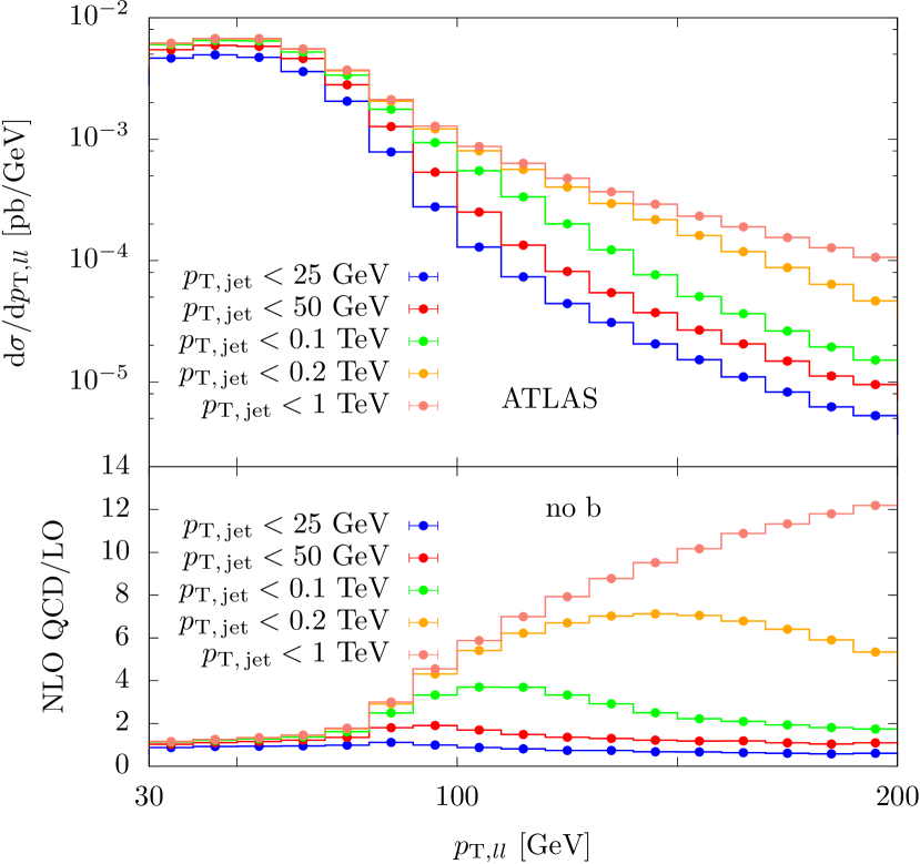
Figure 1: Differential distribution in the transverse momentum of the hardest lepton ($p_{{\rm T},l}^{\rm max}$) and in the $p_{\rm T}$ of the charged-lepton pair ($p_{{\rm T},ll}$) for the process ${\mathrm{p}}{\mathrm{p}}\to{\mathrm{e^{+}}}\nu_{\mathrm{e}}{\mathrm{\mu^{-}}}\bar{\nu}_{\mu}$ at $\sqrt{s}=13\,\mathrm{TeV}$ under the event selections of Eq. (4.4) for different values of the jet $p_{\rm T}$ entering the veto condition in Eq. (4.4). Lower panels: ratio between the NLO QCD and the LO predictions (the same PDF set is used at LO and NLO QCD). The contribution from initial-state ${\mathrm{b}}$ quarks is not included.

Our predictions at the differential-distribution level are collected in Figs. 2–6 for some sample observables. Figures 2–6 confirm the pattern described above at the cross-section level: both the EW and QCD corrections are small in those bins that give the largest contribution to the integrated cross section, while their size increases in the high-$p_{\rm T}$ and invariant-mass regions.

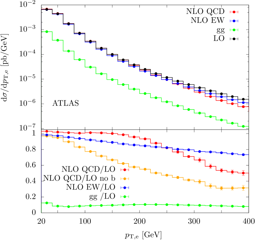
Figure 2: Differential distributions in the transverse momentum of the positron ($p_{{\rm T},{\mathrm{e}}}$) for the process ${\mathrm{p}}{\mathrm{p}}\to{\mathrm{e^{+}}}\nu_{\mathrm{e}}{\mathrm{\mu^{-}}}\bar{\nu}_{\mu}$ at $\sqrt{s}=13\,\mathrm{TeV}$ for the ATLAS and CMS event selections of Eqs. (4.4) and (4.5), respectively. The LO results (black lines) are compared to the ones at NLO QCD (red lines) and NLO EW (blue lines). The ${\mathrm{g}}{\mathrm{g}}$ contribution is also shown (green lines). Lower panels: ratio of the NLO QCD, NLO EW and ${\mathrm{g}}{\mathrm{g}}$ contributions with respect to the LO (red, blue and green lines, respectively). The orange lines correspond to the ratio of the NLO QCD corrections and the LO predictions if the processes with initial-state ${\mathrm{b}}$ quarks are not included (see text for details). For all curves the central value of the factorization and renormalization scales is used and the error bars correspond to the statistical integration uncertainties. Note that the same PDF set is employed for both the LO and NLO predictions.

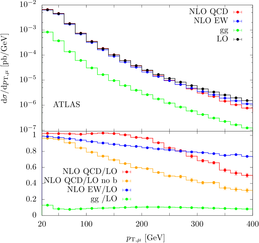
Figure 3: Differential distributions in the transverse momentum of the muon ($p_{{\rm T},\mu}$) for the process ${\mathrm{p}}{\mathrm{p}}\to{\mathrm{e^{+}}}\nu_{\mathrm{e}}{\mathrm{\mu^{-}}}\bar{\nu}_{\mu}$ at $\sqrt{s}=13\,\mathrm{TeV}$ for the ATLAS and CMS event selections of Eqs. (4.4) and (4.5), respectively. Same notations and conventions as in Fig. 2.

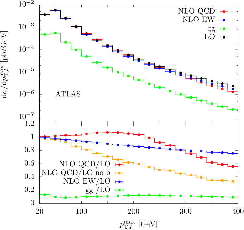
Figure 4: Differential distribution in the transverse momentum of the hardest lepton ($p_{{\rm T},l}^{\rm max}$) and in the invariant mass of the charged-lepton pair ($M^{\rm inv}_{ll}$) for the process ${\mathrm{p}}{\mathrm{p}}\to{\mathrm{e^{+}}}\nu_{\mathrm{e}}{\mathrm{\mu^{-}}}\bar{\nu}_{\mu}$ at $\sqrt{s}=13\,\mathrm{TeV}$ under the event selections of Eqs. (4.4) and (4.5). Same notations and conventions as in Fig. 2.

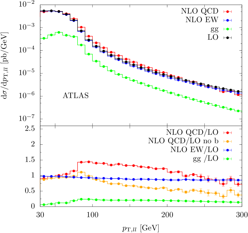
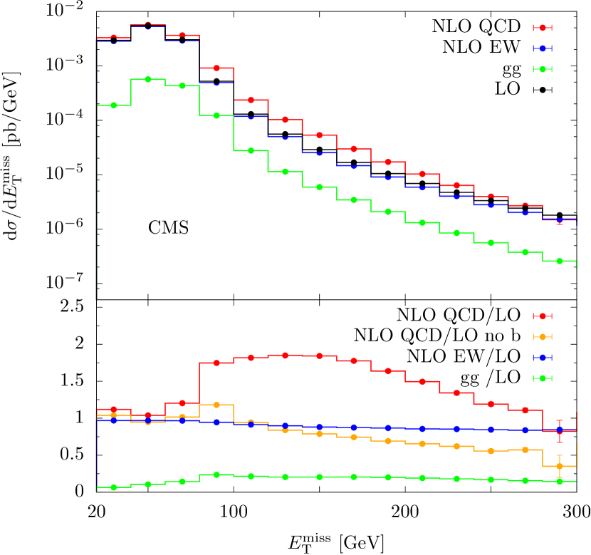
Figure 5: Differential distribution in the transverse momentum of the charged-lepton pair ($p_{{\rm T},ll}$) and in the missing transverse momentum ($E_{{\mathrm{T}}}^{\rm miss}$) for the process ${\mathrm{p}}{\mathrm{p}}\to{\mathrm{e^{+}}}\nu_{\mathrm{e}}{\mathrm{\mu^{-}}}\bar{\nu}_{\mu}$ at $\sqrt{s}=13\,\mathrm{TeV}$ under the event selections of Eqs. (4.4) and (4.5). Same notations and conventions as in Fig. 2.

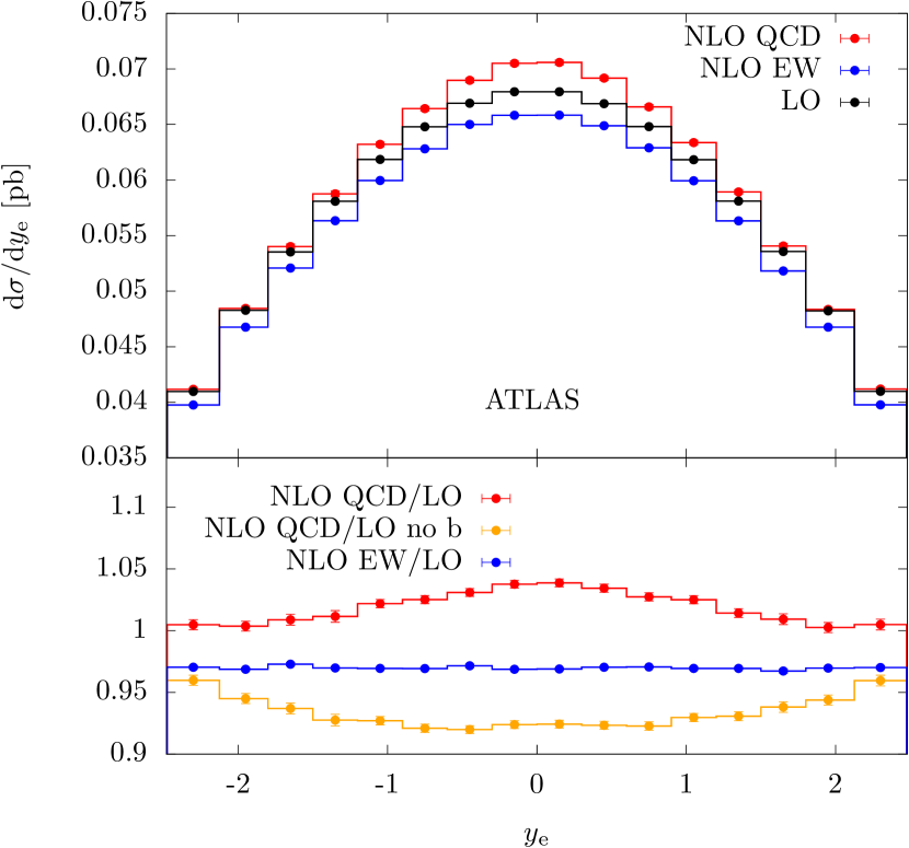
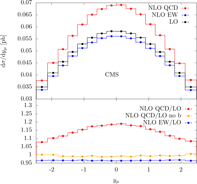
Figure 6: Differential distribution in the positron and muon rapidities ($y_{\rm e}$ and $y_{\mu}$, respectively) for the process ${\mathrm{p}}{\mathrm{p}}\to{\mathrm{e^{+}}}\nu_{\mathrm{e}}{\mathrm{\mu^{-}}}\bar{\nu}_{\mu}$ at $\sqrt{s}=13\,\mathrm{TeV}$ under the event selections of Eqs. (4.4) and (4.5). Same notations and conventions as in Fig. 2. The ${\mathrm{g}}{\mathrm{g}}$ channel gives a flat contribution of a few percent and is not shown to improve the plot readability.

The distributions in the transverse momenta of the positron, muon, and hardest lepton ($p_{\rm T,{\mathrm{e}}}$, $p_{\rm T,\mu}$, and $p_{\rm T,l}^{\mathrm{max}}$, respectively), as well as in the invariant mass of the charged lepton pair $M^{\rm inv}_{ll}$ are shown in Figs. 2–4. For these observables the NLO EW corrections decrease monotonically and become of order $-20\%$ in the tails of the distributions. If the processes with initial-state ${\mathrm{b}}$ quarks are not considered, the NLO QCD corrections behave similar as the NLO EW ones and reach $-60\%$ to $-70\%$ for $p_{\rm T}\simeq 400\,\mathrm{GeV}$ and $M^{\rm inv}_{ll}\simeq 1.2\,\mathrm{TeV}$. The contribution of initial-state ${\mathrm{b}}$ quarks is positive and mainly concentrated in the region between $100$ and $300\,\mathrm{GeV}$ in the $p_{\rm T}$ distribution ($100$ and $600\,\mathrm{GeV}$ in the $M^{\rm inv}_{ll}$ distribution). By looking at Figs. 2 and 3 we find a large difference in the contribution of the processes with initial-state ${\mathrm{b}}$ quarks to the $p_{\rm T,{\mathrm{e}}}$ (and $p_{\rm T,\mu}$) distributions for the ATLAS and CMS setups: we verified that this effect mainly comes from the difference in the jet veto threshold in Eqs. (4.4) and (4.5). In the $p_{\rm T}$ and $M^{\rm inv}_{ll}$ range considered in Figs. 2–4, the impact of the ${\mathrm{g}}{\mathrm{g}}$ channel is basically one order of magnitude smaller than the LO prediction (except for the first few bins of the $M^{\rm inv}_{ll}$ distribution, where this contribution is of order $20{-}30\%$).

The differential distributions of the charged-lepton-pair transverse momentum ($p_{{\rm T},ll}$) and the missing transverse energy ($E_{{\mathrm{T}}}^{\rm miss}$) are shown in Fig. 5. Since at LO $E_{{\mathrm{T}}}^{\rm miss}=p_{{\rm T},ll}$, these two observables are closely related, and the corresponding NLO corrections are similar. As in the case of the lepton-$p_{\rm T}$ distributions in Figs. 2–4, the NLO EW corrections are negative and their size increases with $p_{{\rm T},ll}$ ($E_{{\mathrm{T}}}^{\rm miss}$) reaching the value of $-15\%$ for $p_{{\rm T},ll},E_{{\mathrm{T}}}^{\rm miss}\simeq 300\,\mathrm{GeV}$. If the processes with initial-state ${\mathrm{b}}$ quarks are not included, the NLO QCD corrections become negative and large (of order $-50\%$) in the tail of the distributions. The peak in the NLO QCD corrections around $90\,\mathrm{GeV}$ is a consequence of the jet veto in Eqs. (4.4)–(4.5): as can be seen in Fig. 1, the position of the peak is shifted to larger $p_{{\rm T},ll}$ values as the jet-$p_{\rm T}$ threshold is increased. A similar feature is there for the initial-state ${\mathrm{b}}$-quark contribution, where the peak is much more pronounced.

Figure 6 shows the differential distributions in the positron and muon rapidities ($y_{{\mathrm{e}}}$ and $y_{\mu}$, respectively). Both EW and QCD corrections are basically flat as a function of the lepton rapidities, while the processes with initial-state ${\mathrm{b}}$ quarks give a larger contribution in the central region.

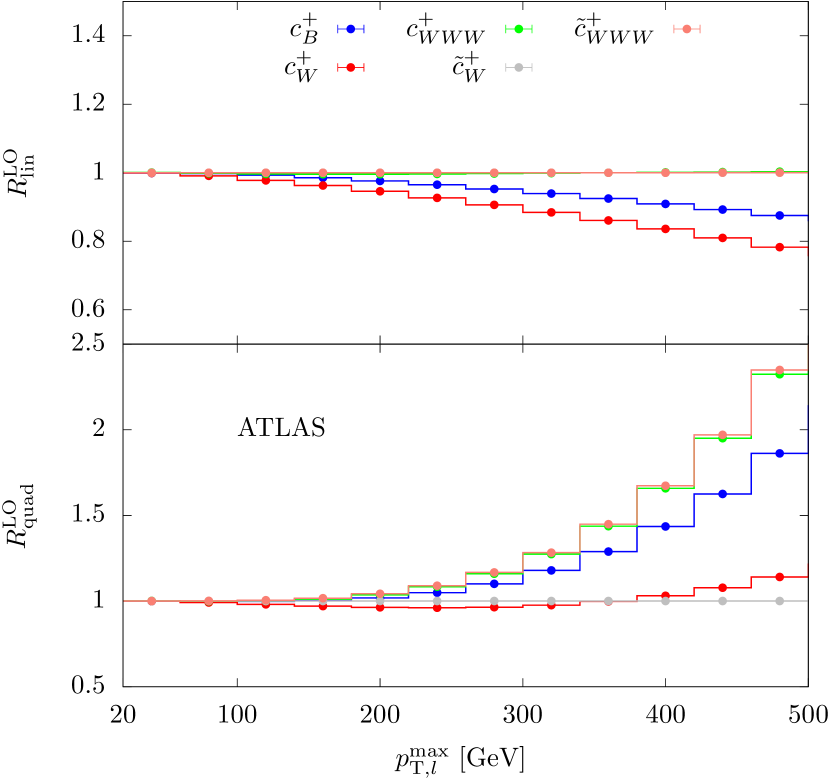
Figure 7: Ratio $R^{\rm LO(NLO)}_{\rm lin(quad)}$ as a function of the transverse momentum of the hardest lepton for the process ${\mathrm{p}}{\mathrm{p}}\to{\mathrm{e^{+}}}\nu_{\mathrm{e}}{\mathrm{\mu^{-}}}\bar{\nu}_{\mu}$ in the ATLAS setup of Eq. (4.4). The ratios between the theoretical predictions including both the aTGCs and the SM results at LO (left plots) are compared to the ratios at NLO QCD accuracy (right plots). In each plot the upper panel corresponds to the ratio where the non-SM contributions are included only up to the interference terms $\sigma^{\rm LO(NLO)}_{{\rm SM}\times{\rm EFT6}}$, while in the lower panel both the $\sigma^{\rm LO(NLO)}_{{\rm SM}\times{\rm EFT6}}$ and the $\sigma^{\rm LO(NLO)}_{{\rm EFT6}^{2}}$ terms are considered. For all curves the central value of the factorization and renormalization scales is used and the error bars correspond to the statistical integration uncertainties.

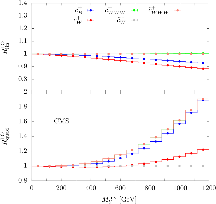
Figure 8: Ratio $R^{\rm LO(NLO)}_{\rm lin(quad)}$ as a function of the invariant mass of the charged-lepton pair for the process ${\mathrm{p}}{\mathrm{p}}\to{\mathrm{e^{+}}}\nu_{\mathrm{e}}{\mathrm{\mu^{-}}}\bar{\nu}_{\mu}$ in the CMS setup of Eq. (4.5). Same notation and conventions as in Fig. 7.

Concerning the impact of the anomalous triple-gauge-boson interactions, we consider the ratios

$$R^{\rm LO(NLO)}_{\rm lin} =\frac{{\rm d}\Big{(}\sigma_{{\rm SM}^{2}}+\sigma_{{\rm SM}\times{\rm EFT}}\Big{)}^{{\rm LO(NLO)}\,{\rm QCD}}/{\rm d}X}{{\rm d}\sigma_{{\rm SM}^{2}}^{{\rm LO(NLO)}\,{\rm QCD}}/{\rm d}X},$$ (5.2)

$$R^{\rm LO(NLO)}_{\rm quad} =\frac{{\rm d}\Big{(}\sigma_{{\rm SM}^{2}}+\sigma_{{\rm SM}\times{\rm EFT}}+\sigma_{{\rm EFT}^{2}}\Big{)}^{{\rm LO(NLO)}\,{\rm QCD}}/{\rm d}X}{{\rm d}\sigma_{{\rm SM}^{2}}^{{\rm LO(NLO)}\,{\rm QCD}}/{\rm d}X},$$

(with $X=p_{{\rm T},l}^{\rm max}\,,M^{\rm inv}_{ll}$) at LO and NLO QCD accuracy. In the $R^{\rm NLO}_{\rm lin\,(quad)}$ ratios the NLO QCD corrections to the diagrams involving the aTGCs are included as well. For the Wilson coefficients we use the values listed in Eq. (3.11). In Figs. 7–8 only one Wilson coefficient is different from zero for each curve. Since the $t$-channel single-top contribution is subtracted in the experimental searches for aTGCs, in Figs. 7–8 the contribution of the processes with initial-state ${\mathrm{b}}$ quarks is not included. Without these processes the NLO QCD corrections become of order $-60\%$ and $-70\%$ for $p_{{\rm T},l}^{\rm max}\simeq 500\,\mathrm{GeV}$ and $M^{\rm inv}_{ll}\simeq 1.2\,\mathrm{TeV}$: we thus limit our analysis to the $p_{{\rm T},l}^{\rm max}$ and $M^{\rm inv}_{ll}$ values below $500\,\mathrm{GeV}$ and $1.2\,\mathrm{TeV}$, respectively, since for larger transverse momenta or invariant masses the differential distributions are strongly suppressed by the NLO QCD corrections.

The impact of aTGCs on the distributions in the transverse momentum of the leading lepton ($p_{{\rm T},l}^{\rm max}$) and the invariant mass of the charged lepton pair ($M^{\rm inv}_{ll}$) at LO is shown in the left plots of Figs. 7–8. Comparing the predictions for $R^{\rm LO}_{\rm lin}$ and $R^{\rm LO}_{\rm quad}$ reveals that the $\sigma^{\rm LO}_{{\rm EFT6}^{2}}$ terms give the largest contribution in the high $p_{\rm T}$ and/or invariant-mass regions. Since the $\sigma^{\rm LO}_{{\rm EFT6}^{2}}$ terms are positive, the results for $R^{\rm LO}_{\rm quad}$ using the two sets $c^{-}$ and $c^{+}$ of Wilson coefficients in Eq. (3.11) are very similar. With the numerical values in Eq. (3.11), the largest deviation from the SM predictions come from the $c_{B}$ and $c_{W}$ coefficients as far as only the $\sigma^{\rm LO}_{{\rm SM}\times{\rm EFT6}}$ interferences are considered, while also the $c_{WWW}$ and $\tilde{c}_{WWW}$ coefficients give a sizable contribution when the $\sigma^{\rm LO}_{{\rm EFT6}^{2}}$ terms are included (the contributions of the $c_{WWW}$ and $\tilde{c}_{WWW}$ coefficients to $R^{\rm LO}_{\rm lin}$ and $R^{\rm LO}_{\rm quad}$ are very similar and the corresponding curves basically overlap in Figs. 7–8).

The results for $R^{\rm NLO}_{\rm lin}$ and $R^{\rm NLO}_{\rm quad}$ are shown in the right plots of Figs. 7–8.

Figure 9: Ratio between the ${\rm EFT6}^{2}$ contribution to the process ${\mathrm{p}}{\mathrm{p}}\to{\mathrm{e^{+}}}\nu_{\mathrm{e}}{\mathrm{\mu^{-}}}\bar{\nu}_{\mu}$ computed at NLO QCD ($\sigma_{{\rm EFT6}^{2}}^{\rm NLO}$) and LO ($\sigma_{{\rm EFT6}^{2}}^{\rm LO}$) accuracy as a function of the hardest lepton $p_{\rm T}$ (left plot) and as a function of the charged-lepton-pair invariant mass. The labels ATLAS and CMS refer to the event selections of Eq. (4.4) and (4.5), respectively. The ratio between the SM predictions at NLO QCD and at LO accuracy is also shown (black lines).

On one hand $R^{\rm NLO}_{\rm lin}$ behaves in a similar way to $R^{\rm LO}_{\rm lin}$, on the other hand the impact of the aTGCs is in general smaller at NLO QCD in particular at high $p_{\rm T}$ and/or invariant masses (with the only exception of the $c_{WWW}$ coefficient that contributes more at NLO QCD). The situation changes for $R^{\rm NLO}_{\rm quad}$, where the sensitivity to the aTGCs is strongly reduced with respect to the LO in particular in the tails of the distributions. At LO the leading contribution to $R^{\rm LO}_{\rm quad}$ is given by the positive and growing $\sigma^{\rm LO}_{{\rm EFT6}^{2}}$ terms. At NLO we have

$$R^{\rm NLO}_{\rm quad}=R^{\rm NLO}_{\rm lin}+\frac{{\rm d}\sigma_{{\rm EFT6}^{2}}^{\rm NLO}}{{\rm d}\sigma_{{\rm SM}^{2}}^{\rm NLO}},$$ (5.3)

where

$$\frac{{\rm d}\sigma_{{\rm EFT6}^{2}}^{\rm NLO}}{{\rm d}\sigma_{{\rm SM}^{2}}^{\rm NLO}}=\frac{{\rm d}\sigma_{{\rm EFT6}^{2}}^{\rm LO}}{{\rm d}\sigma_{{\rm SM}^{2}}^{\rm LO}}\frac{\delta^{\rm QCD}_{{\rm EFT6}^{2}}}{\delta^{\rm QCD}_{\rm SM}},\quad{\rm with}\quad\delta_{{\rm EFT6}^{2}}^{\rm QCD}=\frac{{\rm d}\sigma^{\rm NLO}_{{\rm EFT6}^{2}}}{{\rm d}\sigma^{\rm LO}_{{\rm EFT6}^{2}}},\quad\delta_{\rm SM}^{\rm QCD}=\frac{{\rm d}\sigma^{\rm NLO}_{\rm SM}}{{\rm d}\sigma^{\rm LO}_{\rm SM}}.$$ (5.4)

The NLO QCD corrections suppress the ${\rm EFT6}^{2}$ terms much stronger than the SM contributions as shown in Fig. 9 for the observables under consideration. Figure 9 also reveals why the ${\rm EFT6}^{2}$ contribution is more suppressed for the charged-lepton invariant mass rather than for the hardest lepton $p_{\rm T}$.

Figures 7–8 also show the relative EW NLO corrections determined from the ratio between the NLO EW results and the LO results in the SM. While the introduction of a jet veto is useful to preserve the sensitivity to the aTGCs, it leads to large and negative NLO QCD corrections if the jet veto threshold is small. As a result the effect of the NLO EW corrections is emphasized and can become larger than the one of the aTGCs.

5.2 WZ production

Setup	LO [fb]	NLO QCD [fb]	NLO EW [fb]
${\mathrm{W}}^{-}{\mathrm{Z}}$ ATLAS	$12.6455(9)^{+5.5\%}_{-6.8\%}$	$23.780(4)^{+5.5\%}_{-4.6\%}$	$11.891(4)^{+5.6\%}_{-6.9\%}$
${\mathrm{W}}^{-}{\mathrm{Z}}$ CMS	$~{}9.3251(8)^{+5.3\%}_{-6.7\%}$	$17.215(4)^{+5.4\%}_{-4.3\%}$	$~{}8.870(2)^{+5.5\%}_{-6.7\%}$
${\mathrm{W}}^{+}{\mathrm{Z}}$ ATLAS	$18.875(1)^{+5.2\%}_{-6.4\%}$	$34.253(6)^{+5.3\%}_{-4.3\%}$	$17.748(8)^{+5.3\%}_{-6.5\%}$
${\mathrm{W}}^{+}{\mathrm{Z}}$ CMS	$14.307(1)^{+5.0\%}_{-6.2\%}$	$26.357(6)^{+5.4\%}_{-4.3\%}$	$13.600(4)^{+5.1\%}_{-6.3\%}$

Table 3: Integrated cross section for ${\mathrm{W}}{\mathrm{Z}}$ production at $\sqrt{s}=13\,\mathrm{TeV}$ in the ATLAS and CMS setups of Eqs. (4.7) and (4.8), respectively. In the first column ${\mathrm{W}}^{+}{\mathrm{Z}}$ (${\mathrm{W}}^{-}{\mathrm{Z}}$) is a short-hand notation for the process ${\mathrm{p}}{\mathrm{p}}\to{\mathrm{e^{+}}}\nu_{\rm e}\mu^{+}\mu^{-}$ (${\mathrm{p}}{\mathrm{p}}\to{\mathrm{e^{-}}}\overline{\nu}_{\rm e}\mu^{+}\mu^{-}$). The numbers in parentheses correspond to the statistical error on the last digit. The uncertainties are estimated from the scale dependence, as explained in the text.

The results for the integrated cross sections for WZ production at a centre-of-mass energy of $13\,\mathrm{TeV}$ are presented in Table 3 for the ATLAS and CMS setups of Eqs. (4.7) and (4.8), respectively. In Table 3 and Figs. 10–14,${\mathrm{W}}^{+}{\mathrm{Z}}$ (${\mathrm{W}}^{-}{\mathrm{Z}}$) is a short-hand notation for the process ${\mathrm{p}}{\mathrm{p}}\to{\mathrm{e^{+}}}\nu_{\rm e}\mu^{+}\mu^{-}$ (${\mathrm{p}}{\mathrm{p}}\to{\mathrm{e^{-}}}\overline{\nu}_{\rm e}\mu^{+}\mu^{-}$). The LO predictions are compared to the ones at NLO QCD and NLO EW accuracy. The numbers in parentheses correspond to the statistical integration error, while the upper and lower values of the cross sections correspond to the upper and lower limits from scale variations (5.1). Scale uncertainties are of the same order at LO and NLO EW and do not decrease significantly at NLO QCD as a consequence of the large QCD corrections.

The cross sections for the ${\mathrm{W}}^{+}{\mathrm{Z}}$ channel are about $50\%$ larger than the ones for the ${\mathrm{W}}^{-}{\mathrm{Z}}$ channel: this can be attributed to the parton flux within the proton which is larger for the up quark than for the down quark. The NLO EW corrections are of order $-6\%$ and $-5\%$ in the ATLAS and CMS setups, respectively. The NLO QCD corrections are positive and reach the value of $+80\%$ and $+90\%$, depending on the setup. This is due to the fact that diboson production at LO only proceeds via quark–antiquark annihilation, while at NLO QCD new channels appear that involve initial-state gluons (namely ${\mathrm{g}}q\to{\mathrm{Z}}{\mathrm{W}}^{\pm}q^{\prime}$ and ${\mathrm{g}}\overline{q}\to{\mathrm{Z}}{\mathrm{W}}^{\pm}\overline{q}^{\prime}$) and are enhanced because of the gluon luminosity. In principle, the same happens also for ${\mathrm{W}}{\mathrm{W}}$ production. However, the jet veto in the event selections  (4.4) and (4.5) strongly suppresses the real QCD corrections and in particular the contributions of the processes with initial-state gluons: this explains the different behaviour of NLO QCD corrections for ${\mathrm{W}}{\mathrm{W}}$ and ${\mathrm{W}}{\mathrm{Z}}$ shown in Tables 1 and 3.

Figure 10: Upper panels: differential distributions in the transverse momentum of the positron ($p_{{\rm T},{\mathrm{e}}^{+}}$) and the antimuon ($p_{{\rm T},\mu^{+}}$) for the process ${\mathrm{p}}{\mathrm{p}}\to{\mathrm{e^{+}}}\nu_{\rm e}\mu^{+}\mu^{-}$ at $\sqrt{s}=13\,\mathrm{TeV}$ for the ATLAS and CMS event selections of Eqs. (4.7) and (4.8), respectively. The LO results (black lines) are compared to the ones at NLO QCD (red lines) and NLO EW (blue lines). Lower panels: ratio of the NLO QCD, and NLO EW contributions with respect to the LO (red and blue lines, respectively). In order to improve the plot readability the NLO QCD predictions have been divided by a factor 10 in the ratio ${\rm NLO\,QCD}/{\rm LO}$. For all curves the central value of the factorization and renormalization scales is used and the error bars correspond to the statistical integration uncertainties. Note that the same PDF set is employed for both the LO and NLO predictions.

Figure 11: Differential distribution in the transverse momentum of the muon–antimuon pair ($p_{{\rm T,}\mu^{+}\mu^{-}}$) and in the ${\mathrm{W}}{\mathrm{Z}}$ transverse mass ($M_{\rm T}^{3l\nu}$) for the process ${\mathrm{p}}{\mathrm{p}}\to{\mathrm{e^{+}}}\nu_{\rm e}\mu^{+}\mu^{-}$ at $\sqrt{s}=13\,\mathrm{TeV}$ under the event selections of Eqs. (4.8) and (4.7). The NLO QCD predictions have been divided by a factor 10 (2) in the ratio ${\rm NLO\,QCD}/{\rm LO}$ as a function of $p_{{\rm T,}\mu^{+}\mu^{-}}$ ($M_{\rm T}^{3l\nu}$). Same notations and conventions as in Fig. 10.

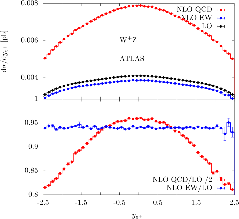
Figure 12: Differential distribution in the positron and antimuon rapidities ($y_{{\rm e}^{+}}$ and $y_{\mu^{+}}$, respectively) for the process ${\mathrm{p}}{\mathrm{p}}\to{\mathrm{e^{+}}}\nu_{\rm e}\mu^{+}\mu^{-}$ at $\sqrt{s}=13\,\mathrm{TeV}$ under the event selections of Eqs. (4.7) and (4.8). Note that the NLO QCD predictions have been divided by a factor 2 in the ratio ${\rm NLO\,QCD}/{\rm LO}$. Same notations and conventions as in Fig. 10.

In Figs. 10–13 we collect results for differential distributions for the process ${\mathrm{p}}{\mathrm{p}}\to{\mathrm{e^{+}}}\nu_{\rm e}\mu^{+}\mu^{-}$. The distributions in the transverse momentum of the positron ($p_{{\rm T},{\mathrm{e}}^{+}}$), the antimuon ($p_{{\rm T},\mu^{+}}$), and the muon–antimuon pair ($p_{{\rm T,}\mu^{+}\mu^{-}}$, i.e. the ${\mathrm{Z}}$-boson transverse momentum) are shown in Figs. 10 and 11. For these distributions the NLO EW corrections are negative and show the typical Sudakov behaviour above about $100\,\mathrm{GeV}$ where they start to decrease monotonically and become of order $-23/{-25}\%$ in the tails of the distributions under consideration. The NLO QCD corrections are positive, large, and increasing for large $p_{\rm T}$. These corrections are dominated by real QCD contributions as has been verified by playing with jet veto cuts. In the presence of hard QCD radiation the four-lepton system recoils against the radiated parton, and the leptons can likely acquire large transverse momentum. Note that in the plots the NLO QCD corrections have been divided by a factor 10.

The right plot in Fig. 11 shows the differential distribution in the transverse mass of the ${\mathrm{W}}{\mathrm{Z}}$ system defined as:

$$M_{{\mathrm{T}}}^{3l\nu}=\sqrt{\left(\sum_{\ell_{i}=1}^{3}p_{\rm T,\ell_{i}}+|\vec{p}_{{\mathrm{T}}}^{\,\rm miss}|\right)^{2}-\left[\left(\sum_{\ell_{i}=1}^{3}p_{\ell_{i},_{x}}+p_{x}^{\rm miss}\right)^{2}+\left(\sum_{\ell_{i}=1}^{3}p_{\ell_{i},_{y}}+p_{y}^{\rm miss}\right)^{2}\,\right]}.$$ (5.5)

As described in Ref. [111], the NLO EW corrections are dominated by the real photon radiation below the peak, then show a plateau between the peak and about $300\,\mathrm{GeV}$ (where they are of order $-5\%$), while for larger $M_{\rm T}^{3l\nu}$ values they decrease up to $-20\%$ for $M_{\rm T}^{3l\nu}=1\,\mathrm{TeV}$. Compared to the transverse momentum distributions, the $M_{\rm T}^{3l\nu}$ observable is less affected by NLO QCD corrections: these contributions are positive, reach the order of $+135\%$ for $M_{\rm T}^{3l\nu}$ around $500\,\mathrm{GeV}$ and then start to slowly decrease.

Figure 12 shows the differential distributions in the positron and the antimuon rapidities ($y_{{\rm e}^{+}}$ and $y_{\mu^{+}}$, respectively). The NLO EW corrections are basically flat and of the same order as the NLO EW corrections to the integrated cross section. The NLO QCD corrections are positive, slightly more pronounced in the central region and again of the same order as the NLO QCD corrections to the integrated cross section.

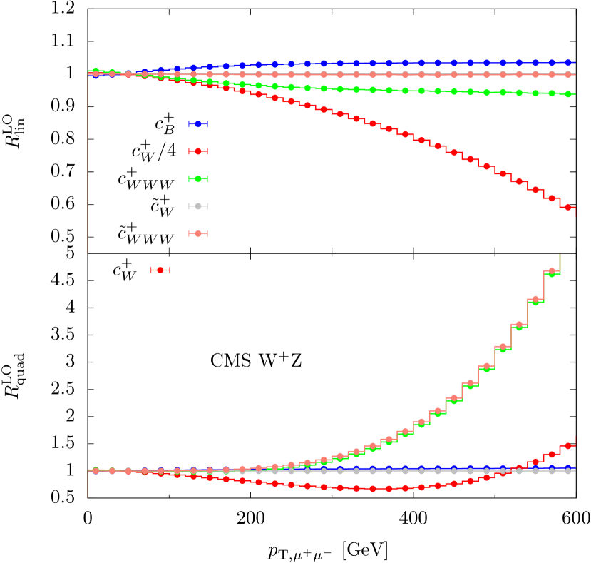
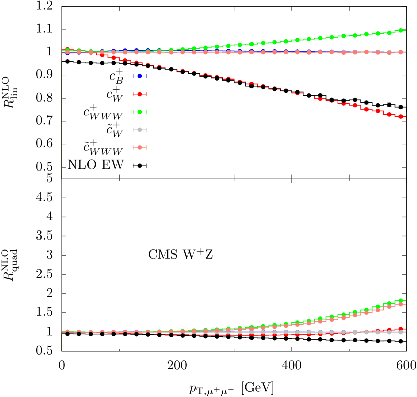
Figure 13: Ratio $R^{\rm LO(NLO)}_{\rm lin(quad)}$ as a function of the muon–antimuon transverse momentum for the process ${\mathrm{p}}{\mathrm{p}}\to{\mathrm{e^{+}}}\nu_{\rm e}\mu^{+}\mu^{-}$ in the CMS setup of Eq. (4.8). Same notation and conventions as in Fig. 7. In order to improve the plot readability, in the $R^{\rm LO}_{\rm lin}$ ratio (upper panels, left plots) the curves labelled with $c_{W}^{\pm}/4$ correspond to our predictions where the $c_{W}^{\pm}$ coefficients in Eq. (3.11) have been divided by a factor 4.

Figure 14: Ratio $R^{\rm LO(NLO)}_{\rm lin(quad)}$ as a function of the ${\mathrm{W}}{\mathrm{Z}}$ transverse mass for the process ${\mathrm{p}}{\mathrm{p}}\to{\mathrm{e^{+}}}\nu_{\rm e}\mu^{+}\mu^{-}$ in the ATLAS setup of Eq. (4.7). Same notation and conventions as in Fig. 7. In order to improve the plot readability, in the $R^{\rm LO}_{\rm lin}$ ratio (upper panels, left plots) the curves labelled with $c_{W}^{\pm}/2$ correspond to our predictions where the $c_{W}^{\pm}$ coefficients in Eq. (3.11) have been divided by a factor 2.

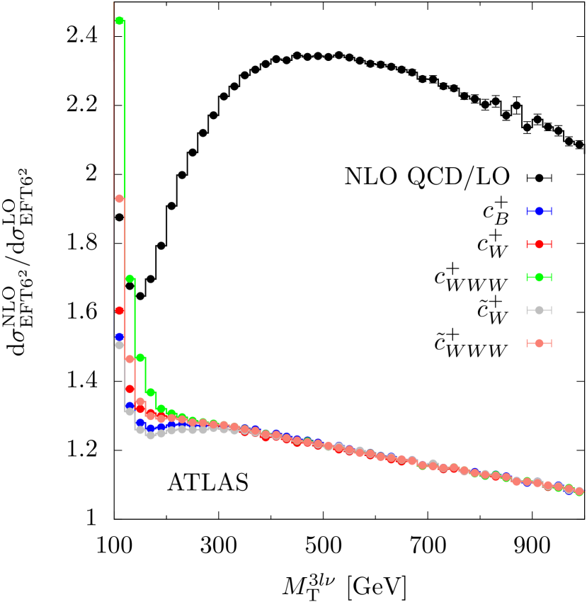
Figure 15: Ratio between the ${\rm EFT6}^{2}$ contribution to the process ${\mathrm{p}}{\mathrm{p}}\to{\mathrm{e^{+}}}\nu_{\rm e}\mu^{+}\mu^{-}$ computed at NLO QCD ($\sigma_{{\rm EFT6}^{2}}^{\rm NLO}$) and LO ($\sigma_{{\rm EFT6}^{2}}^{\rm LO}$) accuracy as a function of the ${\mathrm{W}}{\mathrm{Z}}$ transverse mass (left plot) and as a function of the transverse momentum of the muon–antimuon pair. The labels ATLAS and CMS refer to the event selections of Eq. (4.7) and (4.8), respectively. The ratio between the SM predictions at NLO QCD and at LO accuracy is also shown (black lines).

The ratios $R^{\rm LO(NLO)}_{\rm lin(quad)}$, defined in Eq. (5.2), are shown in Figs. 13 and 14 as a function of the ${\mathrm{Z}}$-boson transverse momentum ($p_{{\rm T,}\mu^{+}\mu^{-}}$) and as a function of the ${\mathrm{W}}{\mathrm{Z}}$ transverse mass ($M_{\rm T}^{3l\nu}$). As in Figs. 7 and 8 we use the values in Eq. (3.11) for the Wilson coefficients, and only one Wilson coefficient is different from zero for each curve. From a qualitative point of view, Figs. 13 and 14 show the same behaviour for $R^{\rm LO}_{\rm lin}$, $R^{\rm LO}_{\rm quad}$, and $R^{\rm NLO}_{\rm lin}$ as Figs. 7 and 8 for ${\mathrm{W}}{\mathrm{W}}$ production. On one hand, by comparing the upper and lower panels of the left plots in Figs. 13–14 we conclude that the largest contribution comes from the $\sigma^{\rm LO}_{{\rm EFT6}^{2}}$ terms (with the only exception of the $c_{W}$ coefficient, for which the $\sigma^{\rm LO}_{{\rm EFT6}^{2}}$ terms become larger than the interference terms only in the tails of the distributions under consideration). On the other hand, comparing the left and the right plots in Figs. 13–14 reveals that the NLO QCD corrections tend to reduce the sensitivity to the aTGCs (with the exception of the $c_{WWW}$ coefficient in $R^{\rm NLO}_{\rm lin}$) in particular for the $R^{\rm NLO}_{\rm quad}$ ratio. Even though $R^{\rm LO}_{\rm lin(quad)}$ and $R^{\rm NLO}_{\rm lin}$ show the same qualitative behaviour for ${\mathrm{W}}{\mathrm{W}}$ and ${\mathrm{W}}{\mathrm{Z}}$ production, from a quantitative point of view we notice that ${\mathrm{W}}{\mathrm{Z}}$ production is more sensitive to aTGCs and in particular to the $c_{W}$ coefficient.

The shape of the $R^{\rm NLO}_{\rm quad}$ distribution can be understood by looking at the NLO QCD corrections to the ${\rm EFT6}^{2}$ contributions (Fig. 15) and Eqs. (5.3) and (5.4). At variance with the ${\mathrm{W}}{\mathrm{W}}$ case, where the jet veto in the event selections (4.4), (4.5) suppresses real QCD radiation, for ${\mathrm{W}}{\mathrm{Z}}$ production the NLO QCD corrections to the ${\rm EFT6}^{2}$ contributions are positive and large owing to real-radiation corrections but much smaller than the corrections to the SM process (this is particularly evident for the $p_{{\rm T,}\mu^{+}\mu^{-}}$ distribution). This is due to the fact that QCD radiation reduces the centre-of-mass energy of the diboson system with respect to the LO. Since the aTGCs contribution increases with the centre-of-mass energy of the diboson system, at NLO QCD the aTGCs contribution is suppressed.

5.3 ZZ production

The results for the fiducial cross sections for the process ${\mathrm{p}}{\mathrm{p}}\to{\mathrm{e^{+}}}{\mathrm{e^{-}}}\mu^{+}\mu^{-}$ at $13\,\mathrm{TeV}$ under the event selection of Eq. (4.11) are collected in Table 4. The LO results are compared to the predictions at NLO QCD and NLO EW accuracy. The contribution of the loop-induced process ${\mathrm{g}}{\mathrm{g}}\to{\mathrm{Z}}{\mathrm{Z}}$ is also shown. The NLO EW corrections are of order $-8\%$ while the NLO QCD corrections amount to $+35\%$. The ${\mathrm{g}}{\mathrm{g}}$ channel contributes about $+17\%$ of the LO prediction. For massless quarks the ${\mathrm{g}}{\mathrm{g}}$ channel results only from quark-box diagrams, while for the massive top quark also $s$-channel Higgs production via a top loop contributes. For a light top quark the contribution of the ${\mathrm{g}}{\mathrm{g}}$ channel amounts to $+24\%$ of the LO cross section, i.e. the large top mass reduces the cross section by $7\%$. The numbers in parentheses represent the integration error on the last digit, while the upper and lower values for the cross sections correspond to the uncertainty coming from scale variation according to Eq. (5.1). Scale uncertainties are of the same order for the LO and the NLO EW predictions and are reduced by a factor of two at NLO QCD.

LO [fb]	NLO QCD [fb]	NLO EW [fb]	${\mathrm{g}}{\mathrm{g}}$ [fb]
$11.0768(5)^{+6.3\%}_{-7.5\%}$	$14.993(2)^{+3.1\%}_{-2.4\%}$	$10.283(2)^{+6.4\%}_{-7.6\%}$	$1.8584(4)^{+25\%}_{-18\%}$

Table 4: Fiducial cross section for the process ${\mathrm{p}}{\mathrm{p}}\to{\mathrm{e^{+}}}{\mathrm{e^{-}}}\mu^{+}\mu^{-}$ at $\sqrt{s}=13\,\mathrm{TeV}$ in the setup of Eqs. (4.11). The numbers in parentheses correspond to the statistical error on the last digit. The uncertainties are estimated from the scale dependence, as explained in the text.

The differential distribution in the transverse momentum of the positron ($p_{{\rm T,e}^{+}}$), the antimuon ($p_{{\rm T,}\mu^{+}}$), the muon–antimuon pair ($p_{{\rm T,}\mu^{+}\mu^{-}}$), and the hardest ${\mathrm{Z}}$ boson [$p_{\rm T,Z}^{\rm max}=\max(p_{{\rm T},\mu^{+}\mu^{-}},\,$ $p_{{\rm T},{\mathrm{e}}^{+}{\mathrm{e}}^{-}})$] are shown in Figs. 16 and 17. For these distributions the NLO EW corrections are negative and decrease monotonically reaching the value of about $-40\%$ for $p_{{\rm T,e}^{+}}$ and $p_{{\rm T,}\mu^{+}}$ of order $600\,\mathrm{GeV}$ and $-50\%$ for $p_{{\rm T,}\mu^{+}\mu^{-}}$ and $p_{\rm T,Z}^{\rm max}$ of order $800\,\mathrm{GeV}$. The NLO QCD corrections are positive, large, and increase at high $p_{\rm T}$. As pointed out in Section 5.2, this is due to the opening of the gluon-initiated channels that contribute to the real QCD corrections and enhance the high-$p_{\rm T}$ region.

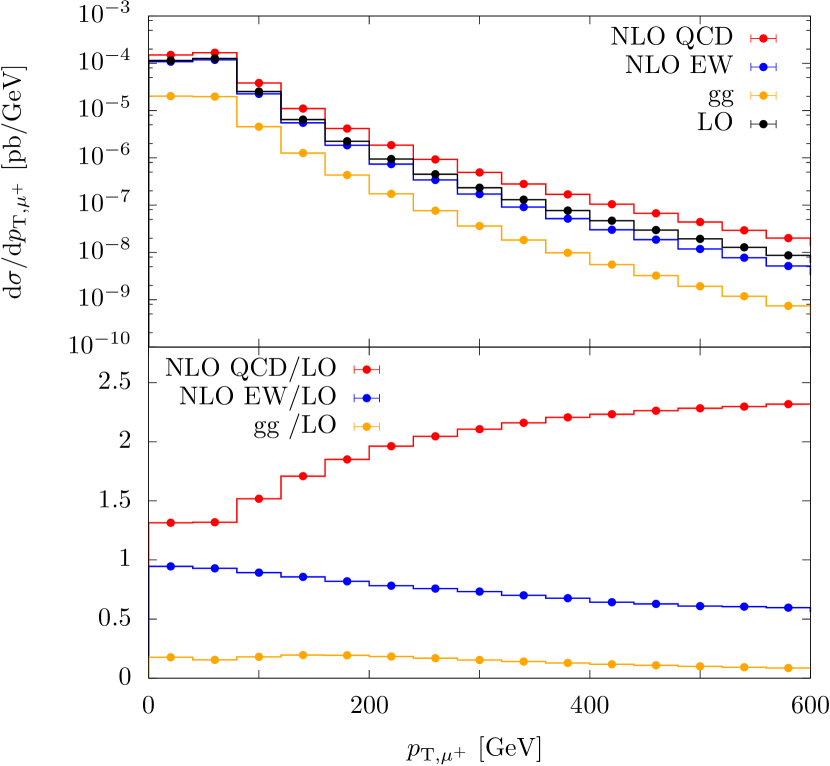
Figure 16: Upper panels: differential distributions in the transverse momentum of the positron ($p_{{\rm T},{\mathrm{e}}^{+}}$) and the antimuon ($p_{{\rm T},\mu^{+}}$) for the process ${\mathrm{p}}{\mathrm{p}}\to{\mathrm{e^{+}}}{\mathrm{e^{-}}}\mu^{+}\mu^{-}$ at $\sqrt{s}=13\,\mathrm{TeV}$ for the event selection of Eq. (4.11). The LO results (black lines) are compared to the ones at NLO QCD (red lines) and NLO EW (blue lines). The ${\mathrm{g}}{\mathrm{g}}$ contribution is also shown (orange lines). Lower panels: ratio of the NLO QCD, NLO EW and ${\mathrm{g}}{\mathrm{g}}$ contributions with respect to the LO (red, blue and orange lines, respectively). For all curves the central value of the factorization and renormalization scales is used and the error bars correspond to the statistical integration uncertainties. Note that the same PDF set is employed for both the LO and NLO predictions.

Figure 17: Differential distribution in the muon–antimuon-pair transverse momentum ($p_{{\rm T},\mu^{+}\mu^{-}}$) and in the hardest ${\mathrm{Z}}$-boson transverse momentum ($p_{{\rm T,\,Z}}^{\rm max}$) for the process ${\mathrm{p}}{\mathrm{p}}\to{\mathrm{e^{+}}}{\mathrm{e^{-}}}\mu^{+}\mu^{-}$ at $\sqrt{s}=13\,\mathrm{TeV}$ under the event selections of Eq. (4.11). Same notations and conventions as in Fig. 16.

Figure 18 shows the differential distributions as a function of the four-lepton invariant mass ($M_{4l}^{\rm inv}$) and as a function of the rapidity difference of the two ${\mathrm{Z}}$ bosons ($\Delta y_{\rm ZZ}$). The $M_{4l}^{\rm inv}$ distribution peaks near $2M_{{\mathrm{Z}}}$: below the peak the NLO EW corrections are dominated by real photon radiation, while above the peak they have the same Sudakov behaviour found in the $p_{\rm T}$ distributions and reach the value of $-45\%$ for $M_{4l}^{\rm inv}$ of order $2\,\mathrm{TeV}$. At variance with the case of the transverse-momentum distributions, the NLO QCD corrections to the four-lepton invariant-mass distribution are relatively flat (they reach the value of $+50\%$ for $M_{4l}^{\rm inv}$ between $0.5$ and $1\,\mathrm{TeV}$ and then they decrease with $M_{4l}^{\rm inv}$). Both the NLO EW and the NLO QCD corrections to the ${\mathrm{Z}}$-boson-pair rapidity difference are essentially flat: the NLO QCD corrections are somewhat larger for large $|\Delta y_{\rm ZZ}|$, while the contribution of the ${\mathrm{g}}{\mathrm{g}}$ channel is of order $+20\%$ for $\Delta y_{\rm ZZ}$ between $-2$ and $2$ and decreases for larger values of $|\Delta y_{\rm ZZ}|$.

Figure 18: Differential distribution in the four-lepton invariant mass ($M_{4l}^{\rm inv}$) and in the ${\mathrm{Z}}$-pair rapidity difference ($\Delta y_{\rm ZZ}$) for the process ${\mathrm{p}}{\mathrm{p}}\to{\mathrm{e^{+}}}{\mathrm{e^{-}}}\mu^{+}\mu^{-}$ at $\sqrt{s}=13\,\mathrm{TeV}$ under the event selections of Eq. (4.11). Same notations and conventions as in Fig. 16.

The differential distributions in the positron and antimuon rapidities ($y_{{\rm e}^{+}}$ and $y_{{\mu}^{+}}$, respectively) are shown in Fig. 19. Both the NLO EW and the NLO QCD corrections are basically flat and of the same order as the corrections to the fiducial cross section.

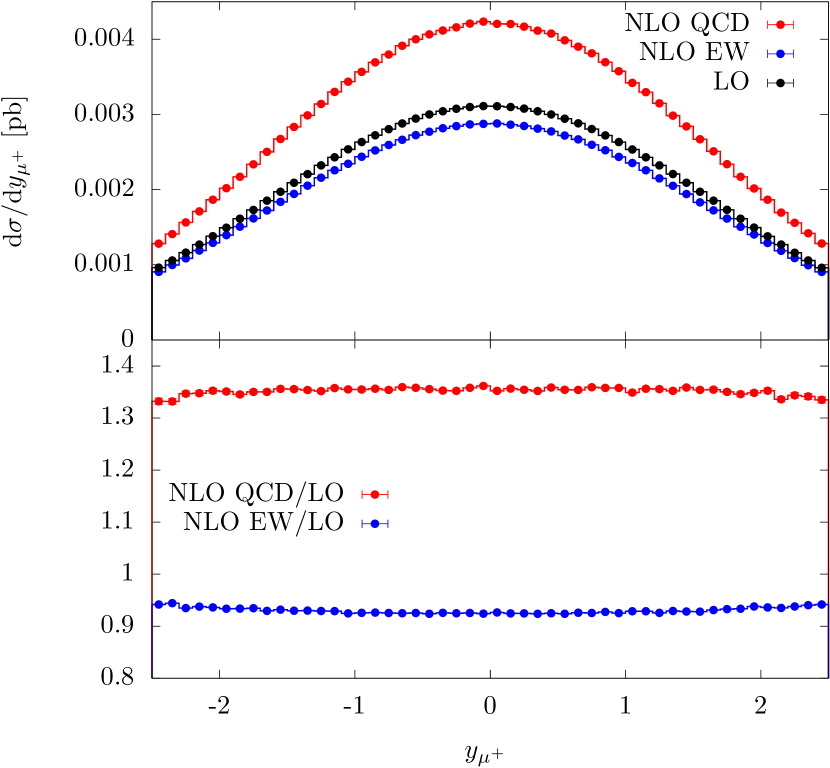
Figure 19: Differential distribution in the positron and antimuon rapidities ($y_{{\rm e}^{+}}$ and $y_{\mu^{+}}$) for the process ${\mathrm{p}}{\mathrm{p}}\to{\mathrm{e^{+}}}{\mathrm{e^{-}}}\mu^{+}\mu^{-}$ at $\sqrt{s}=13\,\mathrm{TeV}$ under the event selections of Eq. (4.11). Same notations and conventions as in Fig. 16.

Concerning the sensitivity to the neutral aTGCs, Figs. 20 and 21 show the differential distribution of the ratios $R^{\rm LO(NLO)}_{\rm lin(quad)}$, defined in Eq. (5.2), as a function of the transverse momentum of the hardest ${\mathrm{Z}}$ boson and as a function of the four-lepton invariant mass. For the Wilson coefficients of the dimension-8 operators involved in ${\mathrm{Z}}{\mathrm{Z}}$ production we use the values listed in Eq. (3.12). As in Figs. 7 and 8, for each curve in the plot only one Wilson coefficient is different from zero. Figures 20 and 21 confirm the same pattern already described for the dimension-6 operators in ${\mathrm{W}}{\mathrm{W}}$ and ${\mathrm{W}}{\mathrm{Z}}$ production. First of all, by comparing $R^{\rm LO(NLO)}_{\rm lin}$ and $R^{\rm LO(NLO)}_{\rm quad}$ we notice that the leading effect comes from the ${\rm EFT}8^{2}$ contributions: this feature is much more evident than in the ${\mathrm{W}}{\mathrm{W}}$ and ${\mathrm{W}}{\mathrm{Z}}$ case, since $R^{\rm LO(NLO)}_{\rm lin}$ turns out to be sensitive only to the $c_{\tilde{B}W}$ coefficient, while for $R^{\rm LO(NLO)}_{\rm quad}$ there is a dependence on all four possible Wilson coefficients. Even for $c_{\tilde{B}W}$, the ${\rm EFT}8^{2}$ contributions always dominate over the ${\rm SM\times EFT8}$ contributions. By comparing $R^{\rm LO}_{\rm lin(quad)}$ and $R^{\rm NLO}_{\rm lin(quad)}$ we conclude that the NLO QCD corrections reduce the dependence on the Wilson coefficients of the dimension-8 operators. For $R^{\rm NLO}_{\rm quad}$ the reduction in the sensitivity to the aTGCs is more pronounced for the $p_{\rm T,Z}^{\rm max}$ observable rather than for the four-lepton invariant-mass distribution. This can be understood by comparing the NLO QCD corrections to the ${\rm EFT}8^{2}$ terms, which furnish the leading contribution to $R^{\rm LO}_{\rm quad}$, with the NLO QCD corrections to the SM results, using equations analogous to Eqs. (5.3) and (5.4).

Figure 20: Ratio $R^{\rm LO(NLO)}_{\rm lin(quad)}$ as a function of the transverse momentum of the hardest ${\mathrm{Z}}$ boson for the process ${\mathrm{p}}{\mathrm{p}}\to{\mathrm{e^{+}}}{\mathrm{e^{-}}}\mu^{+}\mu^{-}$ at $\sqrt{s}=13\,\mathrm{TeV}$ under the event selections of Eq. (4.11). Same notation and conventions as in Fig. 7.

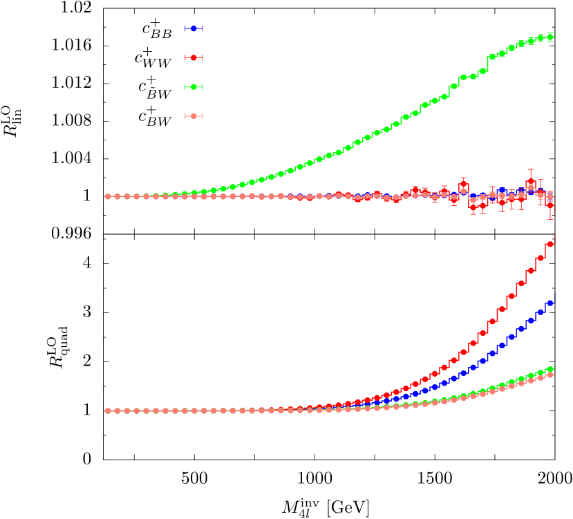
Figure 21: Ratio $R^{\rm LO(NLO)}_{\rm lin(quad)}$ as a function of the four-lepton invariant mass for the process ${\mathrm{p}}{\mathrm{p}}\to{\mathrm{e^{+}}}{\mathrm{e^{-}}}\mu^{+}\mu^{-}$ at $\sqrt{s}=13\,\mathrm{TeV}$ under the event selections of Eq. (4.11). Same notation and conventions as in Fig. 7.

Figure 22: Ratio between the ${\rm EFT8}^{2}$ contribution to the process ${\mathrm{p}}{\mathrm{p}}\to{\mathrm{e^{+}}}\nu_{\rm e}\mu^{+}\mu^{-}$ computed at NLO QCD ($\sigma_{{\rm EFT8}^{2}}^{\rm NLO}$) and LO ($\sigma_{{\rm EFT8}^{2}}^{\rm LO}$) accuracy as a function of the transverse momentum of the hardest ${\mathrm{Z}}$ boson (left plot) and as a function of the four-lepton invariant mass (right plot) under the event selections of Eq. (4.11). The ratio between the SM predictions at NLO QCD and at LO accuracy is also shown (black lines).

The distributions of $\delta_{{\rm EFT8}^{2}}^{\rm QCD}$ and $\delta_{\rm SM}^{\rm QCD}$ are shown in Fig. 22. While for the distribution in the transverse momentum of the leading ${\mathrm{Z}}$ boson we find the same behaviour as already described in Section 5.2 for ${\mathrm{W}}{\mathrm{Z}}$ production, for the distribution in $M_{4l}^{\mathrm{inv}}$ the NLO QCD corrections to the ${\rm EFT}8^{2}$ contribution and the ones to the SM prediction are similar (they differ only by up to $40\%$).

6 Conclusions

A precise theoretical understanding of diboson production processes at the LHC is crucial both in the context of tests of the SM and in the one of the direct searches for anomalous triple-gauge-boson interactions.

In this paper we presented a phenomenological study of ${\mathrm{W}}{\mathrm{W}}$ ($\to{\mathrm{e^{+}}}\nu_{\mathrm{e}}{\mathrm{\mu^{-}}}\bar{\nu}_{\mu}$), ${\mathrm{W}}{\mathrm{Z}}$ ($\to{\mathrm{e^{-}}}\overline{\nu}_{\rm e}\mu^{+}\mu^{-}$), and ${\mathrm{Z}}{\mathrm{Z}}$ ($\to{\mathrm{e^{+}}}{\mathrm{e^{-}}}\mu^{+}\mu^{-}$) production considering event selections of interest for the aTGCs searches at the LHC. For ${\mathrm{W}}{\mathrm{W}}$ and ${\mathrm{Z}}{\mathrm{Z}}$ production we included the impact of the loop-induced ${\mathrm{g}}{\mathrm{g}}\to VV$ processes at LO.

The calculation described in this paper is the first application of Recola2 in the EFT context: a UFO model file including the SM Lagrangian as well as the dimension-6 (-8) operators relevant for ${\mathrm{W}}{\mathrm{W}}$ and ${\mathrm{W}}{\mathrm{Z}}$ (${\mathrm{Z}}{\mathrm{Z}}$) production have been implemented using the Mathematica package FeynRules. The model file has been converted to a Recola2 model file by means of the Python library REPT1L. All NLO QCD and NLO EW corrections in this paper have been computed with Recola2.

The code has been used to study the effect of the aTGCs in the EFT framework at LO and at NLO QCD for some observables of experimental interest. We found that the sensitivity to the aTGCs is in general reduced at NLO QCD because of real radiation contributions, like the opening ${\mathrm{g}}q$/${\mathrm{g}}\overline{q}$ channels, which are less sensitive to the aTGCs. From a quantitative point of view, the reduction in the sensitivity to aTGCs depends on the analysis setup and on the observables under consideration. If the terms involving squared anomalous couplings (${{\rm EFT}^{2}}$ terms) are taken into account, this effect is proportional to the ratio of the NLO QCD corrections to the ${{\rm EFT}^{2}}$ terms and the NLO QCD corrections to the SM predictions. We also disentangled the effect of the interference terms linear in the anomalous couplings (${{\rm SM}\times{\rm EFT}}$) and the ${{\rm EFT}^{2}}$ terms and we showed how the latter dominate over the interference terms almost everywhere in the distributions of interest for the aTGCs searches at the LHC.

Acknowledgements

The work of M.C. and A.D. was supported by the German Science Foundation (DFG) under reference number DE 623/5-1. J.-N. Lang acknowledges support from the Swiss National Science Foundation (SNF) under contract BSCGI0-157722. A.D. and J.-N.L are grateful to the Mainz Institute for Theoretical Physics (MITP) for its hospitality and partial support during the completion of this work.

References

- [1] CDF collaboration, T. Aaltonen et al., Measurement of the production cross section and search for anomalous and couplings in collisions at TeV, Phys. Rev. Lett. 104 (2010) 201801, [0912.4500].
- [2] CDF collaboration, T. Aaltonen et al., Measurement of the cross section and triple gauge couplings in Collisions at TeV, Phys. Rev. D86 (2012) 031104, [1202.6629].
- [3] D0 collaboration, V. M. Abazov et al., Limits on anomalous trilinear gauge boson couplings from , and production in collisions at TeV, Phys. Lett. B718 (2012) 451–459, [1208.5458].
- [4] D0 collaboration, V. M. Abazov et al., Measurement of the production cross section and search for the standard model Higgs boson in the four lepton final state in collisions, Phys. Rev. D88 (2013) 032008, [1304.5422].
- [5] CDF collaboration, T. A. Aaltonen et al., Measurement of the production cross section using the full CDF II data set, Phys. Rev. D89 (2014) 112001, [1403.2300].
- [6] ATLAS collaboration, G. Aad et al., Measurements of production cross sections in collisions at TeV with the ATLAS detector and limits on anomalous gauge boson self-couplings, Phys. Rev. D93 (2016) 092004, [1603.02151].
- [7] ATLAS collaboration, G. Aad et al., Measurement of total and differential production cross sections in proton-proton collisions at 8 TeV with the ATLAS detector and limits on anomalous triple-gauge-boson couplings, JHEP 09 (2016) 029, [1603.01702].
- [8] ATLAS collaboration, M. Aaboud et al., Measurement of the production cross section in proton-proton collisions at 8 TeV using the and channels with the ATLAS detector, JHEP 01 (2017) 099, [1610.07585].
- [9] CMS collaboration, V. Khachatryan et al., Measurement of the cross section in collisions at 8 TeV and limits on anomalous gauge couplings, Eur. Phys. J. C76 (2016) 401, [1507.03268].
- [10] CMS collaboration, V. Khachatryan et al., Measurement of the production cross section and constraints on anomalous triple gauge couplings in four-lepton final states at 8 TeV, Phys. Lett. B740 (2015) 250–272, [1406.0113]. [Erratum: Phys. Lett.B757,569(2016)].
- [11] CMS collaboration, V. Khachatryan et al., Measurements of the production cross sections in the channel in proton–proton collisions at and and combined constraints on triple gauge couplings, Eur. Phys. J. C75 (2015) 511, [1503.05467].
- [12] CMS collaboration, V. Khachatryan et al., Measurement of the production cross section in pp collisions at and 8 TeV and search for anomalous triple gauge couplings at , Eur. Phys. J. C77 (2017) 236, [1609.05721].
- [13] ATLAS collaboration, M. Aaboud et al., Measurement of the production cross section in collisions at a centre-of-mass energy of = 13 TeV with the ATLAS experiment, Phys. Lett. B773 (2017) 354–374, [1702.04519].
- [14] ATLAS collaboration, G. Aad et al., Measurement of the production cross section in collisions at = 13 tev with the ATLAS detector, Phys. Rev. Lett. 116 (2016) 101801, [1512.05314].
- [15] ATLAS collaboration, M. Aaboud et al., Measurement of the boson pair-production cross section in collisions at TeV with the ATLAS Detector, Phys. Lett. B762 (2016) 1–22, [1606.04017].
- [16] CMS collaboration, “Measurement of the cross section collisions at 13 TeV.” CMS-PAS-SMP-16-006, 2016.
- [17] CMS collaboration, V. Khachatryan et al., Measurement of the production cross section and branching fraction in pp collisions at =13 TeV, Phys. Lett. B763 (2016) 280–303, [1607.08834].
- [18] CMS collaboration, V. Khachatryan et al., Measurement of the production cross section in pp collisions at 13 TeV, Phys. Lett. B766 (2017) 268–290, [1607.06943].
- [19] R. W. Brown and K. O. Mikaelian, and pair production in , , colliding beams, Phys. Rev. D19 (1979) 922.
- [20] R. W. Brown, D. Sahdev and K. O. Mikaelian, and pair production in , , and collisions, Phys. Rev. D20 (1979) 1164.
- [21] J. Ohnemus, An order calculation of hadronic production, Phys. Rev. D44 (1991) 3477–3489.
- [22] J. Ohnemus, An order calculation of hadronic production, Phys. Rev. D44 (1991) 1403–1414.
- [23] J. Ohnemus and J. F. Owens, An order calculation of hadronic production, Phys. Rev. D43 (1991) 3626–3639.
- [24] B. Mele, P. Nason and G. Ridolfi, QCD radiative corrections to Z boson pair production in hadronic collisions, Nucl. Phys. B357 (1991) 409–438.
- [25] S. Frixione, P. Nason and G. Ridolfi, Strong corrections to production at hadron colliders, Nucl. Phys. B383 (1992) 3–44.
- [26] S. Frixione, A next-to-leading order calculation of the cross-section for the production of pairs in hadronic collisions, Nucl. Phys. B410 (1993) 280–324.
- [27] F. Cascioli et al., production at hadron colliders in NNLO QCD, Phys. Lett. B735 (2014) 311–313, [1405.2219].
- [28] T. Gehrmann et al., Production at Hadron Colliders in NNLO QCD, Phys. Rev. Lett. 113 (2014) 212001, [1408.5243].
- [29] J. F. Gunion and Z. Kunszt, Lepton correlations in gauge boson pair production and decay, Phys. Rev. D33 (1986) 665.
- [30] J. Ohnemus, Hadronic , , and production with QCD corrections and leptonic decays, Phys. Rev. D50 (1994) 1931–1945, [hep-ph/9403331].
- [31] L. J. Dixon, Z. Kunszt and A. Signer, Vector boson pair production in hadronic collisions at order : Lepton correlations and anomalous couplings, Phys. Rev. D60 (1999) 114037, [hep-ph/9907305].
- [32] J. M. Campbell and R. K. Ellis, An update on vector boson pair production at hadron colliders, Phys. Rev. D60 (1999) 113006, [hep-ph/9905386].
- [33] J. M. Campbell, R. K. Ellis and C. Williams, Vector boson pair production at the LHC, JHEP 07 (2011) 018, [1105.0020].
- [34] M. Grazzini, S. Kallweit and D. Rathlev, production at the LHC: fiducial cross sections and distributions in NNLO QCD, Phys. Lett. B750 (2015) 407–410, [1507.06257].
- [35] M. Grazzini, S. Kallweit, D. Rathlev and M. Wiesemann, production at hadron colliders in NNLO QCD, Phys. Lett. B761 (2016) 179–183, [1604.08576].
- [36] M. Grazzini, S. Kallweit, S. Pozzorini, D. Rathlev and M. Wiesemann, production at the LHC: fiducial cross sections and distributions in NNLO QCD, JHEP 08 (2016) 140, [1605.02716].
- [37] M. Grazzini, S. Kallweit and M. Wiesemann, Fully differential NNLO computations with MATRIX, 1711.06631.
- [38] G. Heinrich, S. Jahn, S. P. Jones, M. Kerner and J. Pires, NNLO predictions for Z-boson pair production at the LHC, 1710.06294.
- [39] S. Dittmaier, S. Kallweit and P. Uwer, NLO QCD corrections to +jet production at hadron colliders, Phys. Rev. Lett. 100 (2008) 062003, [0710.1577].
- [40] J. M. Campbell, R. K. Ellis and G. Zanderighi, Next-to-leading order predictions for jet distributions at the LHC, JHEP 12 (2007) 056, [0710.1832].
- [41] S. Dittmaier, S. Kallweit and P. Uwer, NLO QCD corrections to jet including leptonic -boson decays, Nucl. Phys. B826 (2010) 18–70, [0908.4124].
- [42] T. Binoth, T. Gleisberg, S. Karg, N. Kauer and G. Sanguinetti, NLO QCD corrections to jet production at hadron colliders, Phys. Lett. B683 (2010) 154–159, [0911.3181].
- [43] F. Campanario, C. Englert, S. Kallweit, M. Spannowsky and D. Zeppenfeld, NLO QCD corrections to jet production with leptonic decays, JHEP 07 (2010) 076, [1006.0390].
- [44] Y. Wang, R.-Y. Zhang, W.-G. Ma, X.-Z. Li and L. Guo, QCD and electroweak corrections to jet production with Z-boson leptonic decays at the LHC, Phys. Rev. D94 (2016) 013011, [1604.04080].
- [45] S. Frixione and B. R. Webber, Matching NLO QCD computations and parton shower simulations, JHEP 06 (2002) 029, [hep-ph/0204244].
- [46] P. Nason, A new method for combining NLO QCD with shower Monte Carlo algorithms, JHEP 11 (2004) 040, [hep-ph/0409146].
- [47] S. Frixione, P. Nason and C. Oleari, Matching NLO QCD computations with Parton Shower simulations: the POWHEG method, JHEP 11 (2007) 070, [0709.2092].
- [48] P. Nason and G. Ridolfi, A positive-weight next-to-leading-order Monte Carlo for pair hadroproduction, JHEP 08 (2006) 077, [hep-ph/0606275].
- [49] K. Hamilton, A positive-weight next-to-leading order simulation of weak boson pair production, JHEP 01 (2011) 009, [1009.5391].
- [50] S. Höche, F. Krauss, M. Schönherr and F. Siegert, Automating the POWHEG method in Sherpa, JHEP 04 (2011) 024, [1008.5399].
- [51] T. Melia, P. Nason, R. Röntsch and G. Zanderighi, , and production in the POWHEG BOX, JHEP 11 (2011) 078, [1107.5051].
- [52] P. Nason and G. Zanderighi, , and production in the POWHEG-BOX-V2, Eur. Phys. J. C74 (2014) 2702, [1311.1365].
- [53] F. Cascioli et al., Precise Higgs-background predictions: merging NLO QCD and squared quark-loop corrections to four-lepton jet production, JHEP 01 (2014) 046, [1309.0500].
- [54] T. Gleisberg et al., Event generation with SHERPA 1.1, JHEP 02 (2009) 007, [0811.4622].
- [55] F. Cascioli, P. Maierhöfer and S. Pozzorini, Scattering amplitudes with Open Loops, Phys. Rev. Lett. 108 (2012) 111601, [1111.5206].
- [56] M. Grazzini, S. Kallweit, D. Rathlev and M. Wiesemann, Transverse-momentum resummation for vector-boson pair production at NNLL+NNLO, JHEP 08 (2015) 154, [1507.02565].
- [57] S. Dawson, P. Jaiswal, Y. Li, H. Ramani and M. Zeng, Resummation of jet veto logarithms at N3LLa + NNLO for production at the LHC, Phys. Rev. D94 (2016) 114014, [1606.01034].
- [58] D. A. Dicus, C. Kao and W. W. Repko, Gluon production of gauge bosons, Phys. Rev. D36 (1987) 1570.
- [59] E. W. N. Glover and J. J. van der Bij, Vector boson pair production via gluon fusion, Phys. Lett. B219 (1989) 488–492.
- [60] E. W. N. Glover and J. J. van der Bij, boson pair production via gluon fusion, Nucl. Phys. B321 (1989) 561–590.
- [61] T. Binoth, M. Ciccolini, N. Kauer and M. Krämer, Gluon-induced background to Higgs boson searches at the LHC, JHEP 03 (2005) 065, [hep-ph/0503094].
- [62] C. Zecher, T. Matsuura and J. J. van der Bij, Leptonic signals from off-shell boson pairs at hadron colliders, Z. Phys. C64 (1994) 219–226, [hep-ph/9404295].
- [63] T. Binoth, M. Ciccolini, N. Kauer and M. Krämer, Gluon-induced -boson pair production at the LHC, JHEP 12 (2006) 046, [hep-ph/0611170].
- [64] F. Caola, K. Melnikov, R. Röntsch and L. Tancredi, QCD corrections to production through gluon fusion, Phys. Lett. B754 (2016) 275–280, [1511.08617].
- [65] F. Caola, K. Melnikov, R. Röntsch and L. Tancredi, QCD corrections to production in gluon fusion at the LHC, Phys. Rev. D92 (2015) 094028, [1509.06734].
- [66] S. Alioli, F. Caola, G. Luisoni and R. Röntsch, ZZ production in gluon fusion at NLO matched to parton-shower, Phys. Rev. D95 (2017) 034042, [1609.09719].
- [67] N. Kauer, Interference effects for searches in gluon fusion at the LHC, JHEP 12 (2013) 082, [1310.7011].
- [68] J. M. Campbell, R. K. Ellis and C. Williams, Gluon-gluon contributions to production and Higgs interference effects, JHEP 10 (2011) 005, [1107.5569].
- [69] J. M. Campbell, R. K. Ellis and C. Williams, Bounding the Higgs width at the LHC using full analytic results for , JHEP 04 (2014) 060, [1311.3589].
- [70] N. Kauer and G. Passarino, Inadequacy of zero-width approximation for a light Higgs boson signal, JHEP 08 (2012) 116, [1206.4803].
- [71] N. Kauer, C. O’Brien and E. Vryonidou, Interference effects for and searches in gluon fusion at the LHC, JHEP 10 (2015) 074, [1506.01694].
- [72] J. Bellm et al., Anomalous coupling, top-mass and parton-shower effects in production, JHEP 05 (2016) 106, [1602.05141].
- [73] M. Bonvini, F. Caola, S. Forte, K. Melnikov and G. Ridolfi, Signal-background interference effects for beyond leading order, Phys. Rev. D88 (2013) 034032, [1304.3053].
- [74] F. Caola, M. Dowling, K. Melnikov, R. Röntsch and L. Tancredi, QCD corrections to vector boson pair production in gluon fusion including interference effects with off-shell Higgs at the LHC, JHEP 07 (2016) 087, [1605.04610].
- [75] D. Zeppenfeld and S. Willenbrock, Probing the three-vector-boson vertex at hadron colliders, Phys. Rev. D37 (1988) 1775.
- [76] K. Hagiwara, J. Woodside and D. Zeppenfeld, Measuring the Coupling at the Tevatron, Phys. Rev. D41 (1990) 2113–2119.
- [77] E. Nuss, Diboson production at hadron colliders with general three gauge boson couplings. Analytic expressions of helicity amplitudes and cross-section, Z. Phys. C76 (1997) 701–719, [hep-ph/9610309].
- [78] I. Kuss and E. Nuss, Gauge boson pair production at the LHC: anomalous couplings and vector boson scattering, Eur. Phys. J. C4 (1998) 641–660, [hep-ph/9706406].
- [79] U. Baur and D. L. Rainwater, Probing neutral gauge boson self-interactions in production at hadron colliders, Phys. Rev. D62 (2000) 113011, [hep-ph/0008063].
- [80] U. Baur and D. L. Rainwater, Probing neutral gauge boson self-interactions in production at the Tevatron, Int. J. Mod. Phys. A16S1A (2001) 315–317, [hep-ph/0011016].
- [81] U. Baur, T. Han and J. Ohnemus, production at hadron colliders: effects of nonstandard couplings and QCD corrections, Phys. Rev. D51 (1995) 3381–3407, [hep-ph/9410266].
- [82] U. Baur, T. Han and J. Ohnemus, QCD corrections and nonstandard three vector boson couplings in production at hadron colliders, Phys. Rev. D53 (1996) 1098–1123, [hep-ph/9507336].
- [83] J. Baglio, S. Dawson and I. M. Lewis, An NLO QCD effective field theory analysis of production at the LHC including fermionic operators, Phys. Rev. D96 (2017) 073003, [1708.03332].
- [84] J. M. Campbell and R. K. Ellis, MCFM for the Tevatron and the LHC, Nucl. Phys. Proc. Suppl. 205-206 (2010) 10–15, [1007.3492].
- [85] K. Arnold et al., VBFNLO: a parton level Monte Carlo for processes with electroweak bosons, Comput. Phys. Commun. 180 (2009) 1661–1670, [0811.4559].
- [86] K. Arnold et al., VBFNLO: a parton level Monte Carlo for processes with electroweak bosons – Manual for version 2.5.0, 1107.4038.
- [87] J. Baglio et al., Release Note - VBFNLO 2.7.0, 1404.3940.
- [88] S. Frixione, F. Stoeckli, P. Torrielli, B. R. Webber and C. D. White, The MCaNLO 4.0 Event Generator, 1010.0819.
- [89] J. Alwall, M. Herquet, F. Maltoni, O. Mattelaer and T. Stelzer, MadGraph 5 : going beyond, JHEP 06 (2011) 128, [1106.0522].
- [90] J. Alwall et al., The automated computation of tree-level and next-to-leading order differential cross sections, and their matching to parton shower simulations, JHEP 07 (2014) 079, [1405.0301].
- [91] R. Franceschini, G. Panico, A. Pomarol, F. Riva and A. Wulzer, Electroweak Precision Tests in High-Energy Diboson Processes, 1712.01310.
- [92] W. Beenakker, A. Denner, S. Dittmaier, R. Mertig and T. Sack, High-energy approximation for on-shell W pair production, Nucl.Phys. B410 (1993) 245–279.
- [93] M. Beccaria, G. Montagna, F. Piccinini, F. Renard and C. Verzegnassi, Rising bosonic electroweak virtual effects at high-energy colliders, Phys.Rev. D58 (1998) 093014, [hep-ph/9805250].
- [94] P. Ciafaloni and D. Comelli, Sudakov enhancement of electroweak corrections, Phys. Lett. B446 (1999) 278–284, [hep-ph/9809321].
- [95] J. H. Kühn and A. Penin, Sudakov logarithms in electroweak processes, hep-ph/9906545.
- [96] M. Ciafaloni, P. Ciafaloni and D. Comelli, Bloch-Nordsieck violating electroweak corrections to inclusive TeV scale hard processes, Phys. Rev. Lett. 84 (2000) 4810–4813, [hep-ph/0001142].
- [97] A. Denner and S. Pozzorini, One-loop leading logarithms in electroweak radiative corrections. 1. Results, Eur. Phys. J. C18 (2001) 461–480, [hep-ph/0010201].
- [98] A. Denner and S. Pozzorini, One-loop leading logarithms in electroweak radiative corrections. 2. Factorization of collinear singularities, Eur. Phys. J. C21 (2001) 63–79, [hep-ph/0104127].
- [99] E. Accomando, A. Denner and S. Pozzorini, Electroweak correction effects in gauge-boson pair production at the CERN LHC, Phys. Rev. D65 (2002) 073003, [hep-ph/0110114].
- [100] E. Accomando, A. Denner and A. Kaiser, Logarithmic electroweak corrections to gauge-boson pair production at the LHC, Nucl. Phys. B706 (2005) 325–371, [hep-ph/0409247].
- [101] E. Accomando and A. Kaiser, Electroweak corrections and anomalous triple gauge-boson couplings in and production at the LHC, Phys. Rev. D73 (2006) 093006, [hep-ph/0511088].
- [102] A. Bierweiler, T. Kasprzik, J. H. Kühn and S. Uccirati, Electroweak corrections to -boson pair production at the LHC, JHEP 11 (2012) 093, [1208.3147].
- [103] A. Bierweiler, T. Kasprzik and J. H. Kühn, Vector-boson pair production at the LHC to accuracy, JHEP 12 (2013) 071, [1305.5402].
- [104] J. Baglio, L. D. Ninh and M. M. Weber, Massive gauge boson pair production at the LHC: a next-to-leading order story, Phys. Rev. D88 (2013) 113005, [1307.4331]. [Erratum: Phys. Rev.D94,no.9,099902(2016)].
- [105] M. Billoni, S. Dittmaier, B. Jäger and C. Speckner, Next-to-leading order electroweak corrections to leptons at the LHC in double-pole approximation, JHEP 12 (2013) 043, [1310.1564].
- [106] J. Bellm et al., Herwig 7.0/Herwig++ 3.0 release note, Eur. Phys. J. C76 (2016) 196, [1512.01178].
- [107] S. Gieseke, T. Kasprzik and J. H. Kühn, Vector-boson pair production and electroweak corrections in HERWIG++, Eur. Phys. J. C74 (2014) 2988, [1401.3964].
- [108] B. Biedermann et al., Next-to-leading-order electroweak corrections to 4 leptons at the LHC, JHEP 06 (2016) 065, [1605.03419].
- [109] B. Biedermann, A. Denner, S. Dittmaier, L. Hofer and B. Jäger, Electroweak corrections to at the LHC: a Higgs background study, Phys. Rev. Lett. 116 (2016) 161803, [1601.07787].
- [110] B. Biedermann, A. Denner, S. Dittmaier, L. Hofer and B. Jäger, Next-to-leading-order electroweak corrections to the production of four charged leptons at the LHC, JHEP 01 (2017) 033, [1611.05338].
- [111] B. Biedermann, A. Denner and L. Hofer, Next-to-leading-order electroweak corrections to the production of three charged leptons plus missing energy at the LHC, JHEP 10 (2017) 043, [1708.06938].
- [112] S. Kallweit, J. M. Lindert, S. Pozzorini and M. Schönherr, NLO QCD+EW predictions for diboson signatures at the LHC, JHEP 11 (2017) 120, [1705.00598].
- [113] A. Denner, J.-N. Lang and S. Uccirati, NLO electroweak corrections in extended Higgs Sectors with RECOLA2, JHEP 07 (2017) 087, [1705.06053].
- [114] A. Denner, J.-N. Lang and S. Uccirati, RECOLA2: REcursive Computation of One-Loop Amplitudes 2, Comput. Phys. Commun. 224 (2018) 346–361, [1711.07388].
- [115] N. D. Christensen and C. Duhr, FeynRules - Feynman rules made easy, Comput. Phys. Commun. 180 (2009) 1614–1641, [0806.4194].
- [116] A. Alloul, N. D. Christensen, C. Degrande, C. Duhr and B. Fuks, FeynRules 2.0 - A complete toolbox for tree-level phenomenology, Comput. Phys. Commun. 185 (2014) 2250–2300, [1310.1921].
- [117] A. Denner, Techniques for calculation of electroweak radiative corrections at the one loop level and results for physics at LEP-200, Fortsch. Phys. 41 (1993) 307–420, [0709.1075].
- [118] C. Degrande et al., UFO - The Universal FeynRules Output, Comput. Phys. Commun. 183 (2012) 1201–1214, [1108.2040].
- [119] S. Actis et al., RECOLA: REcursive Computation of One-Loop Amplitudes, Comput. Phys. Commun. 214 (2017) 140–173, [1605.01090].
- [120] A. Denner, S. Dittmaier and L. Hofer, COLLIER: a fortran-based Complex One-Loop LIbrary in Extended Regularizations, Comput. Phys. Commun. 212 (2017) 220–238, [1604.06792].
- [121] F. A. Berends, R. Pittau and R. Kleiss, All electroweak four fermion processes in electron-positron collisions, Nucl. Phys. B424 (1994) 308–342, [hep-ph/9404313].
- [122] S. Dittmaier and M. Roth, LUSIFER: a LUcid approach to six FERmion production, Nucl. Phys. B642 (2002) 307–343, [hep-ph/0206070].
- [123] S. Alioli, P. Nason, C. Oleari and E. Re, A general framework for implementing NLO calculations in shower Monte Carlo programs: the POWHEG BOX, JHEP 06 (2010) 043, [1002.2581].
- [124] L. Barze et al., W production in hadronic collisions using the POWHEG+MiNLO method, JHEP 12 (2014) 039, [1408.5766].
- [125] A. Falkowski, M. Gonzalez-Alonso, A. Greljo, D. Marzocca and M. Son, Anomalous Triple Gauge Couplings in the Effective Field Theory Approach at the LHC, JHEP 02 (2017) 115, [1609.06312].
- [126] K. Hagiwara, S. Ishihara, R. Szalapski and D. Zeppenfeld, Low-energy constraints on electroweak three gauge boson couplings, Phys. Lett. B283 (1992) 353–359.
- [127] K. Hagiwara, S. Ishihara, R. Szalapski and D. Zeppenfeld, Low-energy effects of new interactions in the electroweak boson sector, Phys. Rev. D48 (1993) 2182–2203.
- [128] C. Degrande et al., Effective Field Theory: A Modern Approach to Anomalous Couplings, Annals Phys. 335 (2013) 21–32, [1205.4231].
- [129] C. Degrande et al., Monte Carlo tools for studies of non-standard electroweak gauge boson interactions in multi-boson processes: A Snowmass White Paper, in Proceedings, Community Summer Study 2013: Snowmass on the Mississippi (CSS2013): Minneapolis, MN, USA, July 29-August 6, 2013, 2013, 1309.7890, http://inspirehep.net/record/1256129/files/arXiv:1309.7890.pdf.
- [130] C. Degrande, A basis of dimension-eight operators for anomalous neutral triple gauge boson interactions, JHEP 02 (2014) 101, [1308.6323].
- [131] K. Hagiwara, R. D. Peccei, D. Zeppenfeld and K. Hikasa, Probing the weak boson sector in , Nucl. Phys. B282 (1987) 253–307.
- [132] G. J. Gounaris, J. Layssac and F. M. Renard, Signatures of the anomalous and production at the lepton and hadron colliders, Phys. Rev. D61 (2000) 073013, [hep-ph/9910395].
- [133] A. De Rujula, M. B. Gavela, P. Hernandez and E. Masso, The selfcouplings of vector bosons: Does LEP-1 obviate LEP-2?, Nucl. Phys. B384 (1992) 3–58.
- [134] W. Buchmüller and D. Wyler, Effective lagrangian analysis of new interactions and flavor conservation, Nucl. Phys. B268 (1986) 621–653.
- [135] B. Grzadkowski, M. Iskrzynski, M. Misiak and J. Rosiek, Dimension-Six Terms in the Standard Model Lagrangian, JHEP 10 (2010) 085, [1008.4884].
- [136] K. J. F. Gaemers and G. J. Gounaris, Polarization amplitudes for and , Z. Phys. C1 (1979) 259.
- [137] G. J. Gounaris, J. Layssac and F. M. Renard, Off-shell structure of the anomalous and selfcouplings, Phys. Rev. D62 (2000) 073012, [hep-ph/0005269].
- [138] G. J. Gounaris, J. Layssac and F. M. Renard, New and standard physics contributions to anomalous and selfcouplings, Phys. Rev. D62 (2000) 073013, [hep-ph/0003143].
- [139] A. Biekötter, A. Knochel, M. Krämer, D. Liu and F. Riva, Vices and virtues of Higgs effective field theories at large energy, Phys. Rev. D91 (2015) 055029, [1406.7320].
- [140] R. Contino, A. Falkowski, F. Goertz, C. Grojean and F. Riva, On the validity of the Effective Field Theory approach to SM precision tests, JHEP 07 (2016) 144, [1604.06444].
- [141] CMS collaboration, A. M. Sirunyan et al., Search for anomalous couplings in boosted production in proton-proton collisions at 8 TeV, Phys. Lett. B772 (2017) 21–42, [1703.06095].
- [142] Particle Data Group collaboration, C. Patrignani et al., Review of Particle Physics, Chin. Phys. C40 (2016) 100001.
- [143] D. Yu. Bardin, A. Leike, T. Riemann and M. Sachwitz, Energy Dependent Width Effects in Annihilation Near the Boson Pole, Phys. Lett. B206 (1988) 539–542.
- [144] A. Denner, S. Dittmaier, M. Roth and D. Wackeroth, Predictions for all processes fermions , Nucl. Phys. B560 (1999) 33–65, [hep-ph/9904472].
- [145] A. Denner, S. Dittmaier, M. Roth and L. H. Wieders, Electroweak corrections to charged-current fermion processes: technical details and further results, Nucl. Phys. B724 (2005) 247–294, [hep-ph/0505042]. [Erratum: Nucl. Phys.B854,504(2012)].
- [146] A. Denner and S. Dittmaier, The complex-mass scheme for perturbative calculations with unstable particles, Nucl. Phys. Proc. Suppl. 160 (2006) 22–26, [hep-ph/0605312].
- [147] A. Buckley et al., LHAPDF6: parton density access in the LHC precision era, Eur. Phys. J. C75 (2015) 132, [1412.7420].
- [148] R. D. Ball et al., Parton distributions with LHC data, Nucl. Phys. B867 (2013) 244–289, [1207.1303].
- [149] NNPDF collaboration, R. D. Ball et al., Parton distributions with QED corrections, Nucl. Phys. B877 (2013) 290–320, [1308.0598].
- [150] NNPDF collaboration, R. D. Ball et al., Parton distributions for the LHC Run II, JHEP 04 (2015) 040, [1410.8849].
- [151] M. Cacciari and G. P. Salam, Dispelling the myth for the jet-finder, Phys. Lett. B641 (2006) 57–61, [hep-ph/0512210].
- [152] M. Cacciari, G. P. Salam and G. Soyez, The anti- jet clustering algorithm, JHEP 04 (2008) 063, [0802.1189].
- [153] M. Cacciari, G. P. Salam and G. Soyez, FastJet User Manual, Eur. Phys. J. C72 (2012) 1896, [1111.6097].
- [154] A. Azatov, J. Elias-Miro, Y. Reyimuaji and E. Venturini, Novel measurements of anomalous triple gauge couplings for the LHC, JHEP 10 (2017) 027, [1707.08060].