Nonequilibrium atom-surface interaction with lossy multi-layer structures

Abstract

The impact of lossy multi-layer structures on nonequilibrium atom-surface interactions is discussed. Specifically, the focus lies on a fully non-Markovian and nonequilibrium description of quantum friction, the fluctuation-induced drag force acting on an atom moving at constant velocity and height above the multi-layer structures. Compared to unstructured bulk material, the drag force for multi-layer systems is considerably enhanced and exhibits different regimes in its velocity and distance dependences. These features are linked to the appearance of coupled interface polaritons within the superlattice structures. Our results are not only useful for an experimental investigation of quantum friction but also highlight a way to tailor the interaction by simply modifying the structural composition of the multi-layer systems.

I Introduction

The notion of vacuum changed dramatically after the rise of quantum mechanics. The existence of quantum fluctuations even at zero temperature and the possibility of “structuring the vacuum” has led to the discovery of many new interesting phenomena. In this context many vacuum fluctuation-induced interactions such as the Casimir and Casimir-Polder effect Casimir1948 have been investigated. Strongly related to the Casimir-Polder force, is quantum friction, a drag force that even at zero temperature opposes the relative motion of two or more objects in vacuum Intravaia2016 . One of the most studied configurations consists of an atom (or a microscopic object) moving parallel to a surface at constant height and velocity Intravaia15 ; Pieplow15 ; Dedkov02a ; Scheel2009 . In such a system, quantum friction has a simple interpretation in terms of the interaction between the moving microscopic object and its image within the material below. The motion of the image is “delayed” due to the frequency dispersion of the material permittivity, leading to both a modification of the equilibrium Casimir-Polder force perpendicular to the surface and a component of the force parallel to the surface that opposes the motion. Already in this simple picture, we can intuitively understand the relevance of two mechanisms at work in the quantum frictional process: The strength of the coupling between the microscopic object and its image and the resistance felt by the image when dragged through the material. The latter can be related to the dynamics of the charge carriers within the material composing the substrate and, in particular to its resistivity. Instead, the coupling strength strongly depends on the electromagnetic densities of states characterizing the system. Altering either one of these aspects will eventually lead to an modification of quantum friction. A currently popular class of systems where this can be implemented are nanostructured substrate materials Yan2012 ; Liu2007 ; Shekhar2014 . In the framework of fluctuation-induced forces, they have already been considered both in theoretical analyses (see for example Messina2017 ; Lambrecht2008 ; Rodriguez11 ; Intravaia12a ; Intravaia15 ) and in experiments Chan08 ; Intravaia13 ; Bender14 ; Tang17 ; Chan18 . One prominent example is given by nanoscaled multi-layer structures, where a specific pattern of distinct layers are repeatedly stacked forming a superlattice Saarinen2008 ; Poddubny13 ; Guo14b . When carefully designed, they are known for exhibiting effective hyperbolic dispersion relations Iorsh12 ; Kidwai12 ; Poddubny13 , which have applications in many fields of research Belov06 ; Wurtz11 ; Cortes12 .

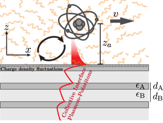
Figure 1: A schematic description of the system considered in this work. An atom (or microscopic object) moves at constant velocity and constant height above a half-space made by periodic sequence of alternating conductive ($\epsilon_{\rm A}$) and dielectric ($\epsilon_{\rm B}$) layers with corresponding thicknesses $d_{\rm A}$ and $d_{\rm B}$. The spectrum of vacuum fluctuations is ”stuctured” through the properties of the multi-layered structure and gives rise to a nonequilibrium atom-surface interaction which opposes the motion of the atom. This quantum frictional force is affected by the appearance of electromagnetic resonances due to the inter-layer interaction of plasmon-polaritons at the dielectric-metal interfaces and can be tailored by acting on the geometry and the material properties of the individual layers.

In the present work, we investigate how the characteristic behavior of quantum friction and specifically its strength and functional dependence on the velocity and position of the atom, is modified when the planar medium is a two-component superlattice of alternating layers with metallic and dielectric properties. The paper is organized as follows. In Section II, we briefly review the theory of quantum friction, highlighting the features connected with the properties of the surface, which can lead to a modification of the interaction through nanostructuring. We introduce in Section III our material models, analyzing the properties and the physical parameters which are relevant to the quantum frictional process. Finally, in Section IV, we merge the insights of the previous two sections and explicitly calculate the quantum frictional force on an atom moving above a superlattice.

II Quantum Friction

Physically, quantum friction can be derived from the Lorentz force: If we choose the $z$-axis to be perpendicular to the surface (see Fig. 1), the force lies in the $(x,y)$-plane against the direction of motion. This means that if the atom moves at constant height $z_{a}$ above a flat surface with constant velocity $\mathbf{v}$, then $\mathbf{F}=F\mathbf{v}/v$ ($v=|\mathbf{v}|$) Intravaia2016 . In our description, the atom is described in terms of a time-dependent dipole operator $\hat{\mathbf{d}}(t)$: For simplicity, we further assume a rigid dipole configuration $\hat{\mathbf{d}}(t)=\mathbf{d}\hat{q}(t)$, where $\mathbf{d}$ is the static dipole vector and $\hat{q}(t)$ describes the dipole’s internal dynamics. For systems at temperature $T=0$, it has been shown Intravaia2014 ; Intravaia2016 that the quantum frictional force $\mathbf{F}$ is given as

$$\mathbf{F} = -2\int_{0}^{\infty}\mathrm{d}\omega\,\int\frac{\mathrm{d}^{2}\mathbf{k}}{(2\pi)^{2}}$$ (1)

$$\times\mathbf{k}\,\mathrm{Tr}\left[\underline{S}(\mathbf{k}\cdot\mathbf{v}-\omega;\mathbf{v})\cdot\underline{G}_{I}(\mathbf{k},z_{a},\omega)\right]\,.$$

Here, $\mathbf{k}$ is the component of the wavevector parallel to the surface, $\underline{G}$ is the Fourier transform with respect to the planar coordinates of the electromagnetic Green tensor. The tensor

$$\underline{S}(\omega)=\frac{1}{2\pi}\int_{-\infty}^{\infty}\mathrm{d}\tau\,e^{i\omega\tau}\,\langle\hat{\mathbf{d}}(\tau)\hat{\mathbf{d}}(0)\rangle_{\mathrm{NESS}}\,$$ (2)

represents the power spectrum corresponding to the dipole-dipole correlator for the system’s nonequilibrium steady state (NESS) and describes the strength of the fluctuations affecting the atomic system. The subscripts “$I$” and “$R$” appearing in the previous and the following expressions denote the real and the imaginary part of the quantities they are appended to (e.g., $\underline{G}_{I}=\mathrm{Im}\{\underline{G}\}$, $\underline{G}_{R}=\mathrm{Re}\{\underline{G}\}$, etc.). Assuming that $\hat{q}(t)$ can be described in terms of a harmonic oscillator, the power spectrum can be written as Intravaia2016a

$$\underline{S}(\omega;\mathbf{v})=\frac{\hbar}{\pi}\theta(\omega)\underline{\alpha}_{I}(\omega;\mathbf{v})\,+\frac{\hbar}{\pi}\underline{J}(\omega;\mathbf{v}),$$ (3)

where $\underline{\alpha}(\omega;\mathbf{v})$ is the velocity-dependent dressed atomic polarizability (see Appendix A). The first term on the r.h.s. corresponds to the result one would obtain using the so-called local thermal equilibrium (LTE) approximation. Within this approximation, it is assumed that the atom is in equilibrium with its immediate surroundings, allowing the application of the fluctuation-dissipation theorem Callen1951 . The “locally equilibrated atom”’ is subsequently coupled to the substrate material. However, a full nonequilibrium description yields the additional term $\underline{J}(\omega;\mathbf{v})$, which substantially contributes to the quantum frictional process (see Appendix A and Refs. Intravaia14 ; Intravaia2016a ; Reiche2017 ).

The physics of quantum friction is connected to that of the quantum Cherenkov effect through the anomalous Doppler effect Pieplow15 ; Maghrebi13a ; Intravaia2016 . In simple terms, we have that, through the Doppler shift appearing in Eq. (1), this process brings negative frequencies of the electromagnetic spectrum into the integration region which is physically relevant for the interaction. Previous work has shown that, depending on the atom’s velocity, quantum friction is characterized by the combination of a non-resonant and a resonant contribution. The resonant part occurs when the system’s resonances, such as atomic transition frequencies or polaritonic surface modes existing at the vacuum/substrate interface, participate in the interaction. Usually, they become relevant only for velocities high enough to generate a Doppler shift, which displaces the resonances into the aforementioned relevant frequency range. As a rough rule of thumb, this occurs for $v/z_{a}>\omega_{\rm r}$, where $\omega_{\rm r}$ is the resonance frequency under consideration. Similarly, the non-resonant part gives the dominant contribution for the force at low velocities and is directly related to the low-frequency optical response of the substrate. Specifically, this region is strongly affected by the dissipative behavior of the material(s) composing the substrate. In this non-resonant regime the force is to a good approximation described by

$$\mathbf{F}\approx -2\frac{\hbar}{\pi}\int\frac{\mathrm{d}^{2}\mathbf{k}}{(2\pi)^{2}}\,\mathbf{k}\,\theta(\mathbf{k}\cdot\mathbf{v})\int\frac{\mathrm{d}^{2}\tilde{\mathbf{k}}}{(2\pi)^{2}}\int_{0}^{\mathbf{k}\cdot\mathbf{v}}\mathrm{d}\omega\,\mathrm{Tr}\left[\underline{\alpha}_{0}\cdot\underline{\sigma}_{I}(\tilde{\mathbf{k}},z_{a},[\mathbf{k}+\tilde{\mathbf{k}}]\cdot\mathbf{v}-\omega)\right]\mathrm{Tr}\left[\underline{\alpha}_{0}\cdot\underline{\sigma}_{I}(\mathbf{k},z_{a},\omega)\right]$$

$$-2\frac{\hbar}{\pi}\int\frac{\mathrm{d}^{2}\mathbf{k}}{(2\pi)^{2}}\,\mathbf{k}\int\frac{\mathrm{d}^{2}\tilde{\mathbf{k}}}{(2\pi)^{2}}\theta(\mathbf{\tilde{k}}\cdot\mathbf{v})\int_{\mathbf{k}\cdot\mathbf{v}}^{[\mathbf{k}+\tilde{\mathbf{k}}]\cdot\mathbf{v}}\mathrm{d}\omega\,\mathrm{Tr}\left[\underline{\alpha}_{0}\cdot\underline{\sigma}_{I}(\tilde{\mathbf{k}},z_{a},[\tilde{\mathbf{k}}+\mathbf{k}]\cdot\mathbf{v}-\omega)\cdot\underline{\alpha}_{0}\cdot\underline{\sigma}_{I}(\mathbf{k},z_{a},\omega)\right].$$ (4)

Here, the dyadic $\underline{\alpha}_{0}=\mathbf{d}\mathbf{d}$ describes the static polarizability for our model. In the above expression we have also used that, due to the properties of the trace and of the polarizability, we can replace the Green tensor by its (symmetric) diagonal part, $\underline{\sigma}(\mathbf{k},z_{a},\omega)$. Since quantum friction strongly decays with increasing atom-surface separation (see also Sec. IV), the dominant contribution of the above expressions come from the system’s near-field region. In this region $\underline{\sigma}(\mathbf{k},z_{a},\omega)$ can be written as

$$\underline{\sigma}(\mathbf{k},z_{a},\omega)\approx r^{p}(\omega,k)\mathrm{diag}\left[\frac{k_{x}^{2}}{k^{2}},\frac{k_{y}^{2}}{k^{2}},1\right]\frac{ke^{-2kz_{a}}}{2\epsilon_{0}}\,.$$ (5)

Here, $\epsilon_{0}$ is the vacuum permittivity, $k=|\mathbf{k}|$ and $r^{p}(\omega,k)$ is the reflection coefficient of the substrate for the $p$-polarized electromagnetic radiation.

The previous equations show that the quantum frictional interaction is mainly connected with the $p$-polarized electromagnetic field (the $s$-polarized field gives a small contribution of the order $v^{2}/c^{2}$, with $c$ the speed of light) and is dominated by wave vectors $k\lesssim 1/z_{a}$ and frequencies $0<\omega\lesssim v/z_{a}$. It is interesting to note that, if in this regime we can write $r^{p}_{I}(\omega,k)\approx 2(\omega\epsilon_{0})^{n}\rho_{n}(k)$, Eq. (4) gives a velocity dependence $F\propto v^{2n+1}$, while the distance dependence is related to the detail of the generalized resistivity $\rho_{n}(k)$. For $n=1$ one speaks of ohmic materials, while $n<1$ and $n>1$ indicate, respectively, sub-ohmic and super-ohmic behavior. This feature has been connected to the non-Markovian properties of the electromagnetic atom-surface interaction Intravaia14 ; Intravaia2016 and explains why many of the authors have obtained $F\propto v^{3}$ for the low-velocity asymptotic expression of the quantum frictional force on an atom moving above a substrate made of a homogeneous (ohmic) material Dedkov02a . Since the nature of the planar medium determines the functional dependence of the force, tailoring the properties of the substrate allows for a control of the interaction.

III Electromagnetic scattering near nano-structures

The above expressions highlight the dependence of the quantum frictional force on the optical response of the substrate and show the important role of the reflection coefficients of the substrate. The literature offers many different approaches for calculating these quantities for nanostructures. However, most of the papers focus on frequency ranges, wave-vectors and, in general, material characteristics which are not those that are relevant for the evaluation of the quantum frictional force. In order to define the notation and give a consistent framework to our considerations, we present in this section an analysis which focuses on these aspects.

We start by considering the expression for the reflection coefficients of a flat surface. In general, they can be written as Ford84

$$r^{\sigma}(\omega,k)=\delta^{\sigma}\frac{Z_{0}^{\sigma}(\omega,k)-Z_{\mathrm{m}}^{\sigma}(\omega,k)}{Z_{0}^{\sigma}(\omega,k)+Z_{\mathrm{m}}^{\sigma}(\omega,k)},$$ (6)

where the index $\sigma=s,p$ denotes the polarization state of light and we have introduced $\delta^{s/p}=\mp$. Further $Z_{\mathrm{m}}^{\sigma}(\omega,k)$ and $Z_{0}^{\sigma}(\omega,k)$ denote, respectively, the surface impedance for the substrate material and the material surrounding it (for simplicity, in the subsequent discussions, we assume this material to be vacuum). The surface reflection coefficients are sensitive to the substrate material properties and the geometry of the system. For our forthcoming analyses, it is interesting to consider first the case of a slab of thickness $D$ suspended in vacuum and made by a homogeneous material characterized by the spatially local complex permittivity function $\epsilon(\omega)$ Note1 . In this case Eq. (6) simplifies as follow Sipe1981

$$r_{\mathrm{slab}}^{\sigma}(\omega,k)=r^{\sigma}_{\mathrm{bulk}}(\omega,k)\frac{1-e^{2ik_{z}D}}{1-[r^{\sigma}_{\mathrm{Bulk}}(\omega,k)e^{ik_{z}D}]^{2}},$$ (7)

where $k_{z}=\sqrt{\epsilon(\omega)\frac{\omega^{2}}{c^{2}}-k^{2}}$ ($\mathrm{Im}\{k_{z}\}\geq 0$, $\mathrm{Re}\{k_{z}\}\geq 0$), and $r^{\sigma}_{\mathrm{Bulk}}(\omega,k)$ is the interface reflection coefficient given by the usual Fresnel expressions Jackson75 . For a spatially local, isotropic and homogenous substrate material we have that the impedance in Eq. (6) can be written as

$$Z_{\mathrm{m}}^{s}(\omega,k)\equiv Z_{\mathrm{bulk}}^{s}(\omega,k)=\frac{\frac{\omega^{2}}{c^{2}}}{\sqrt{\frac{\omega^{2}}{c^{2}}\epsilon(\omega)-k^{2}}},$$ (8a)

$$Z_{\mathrm{m}}^{p}(\omega,k)\equiv Z_{\mathrm{bulk}}^{p}(\omega,k)=\frac{\sqrt{\frac{\omega^{2}}{c^{2}}\epsilon(\omega)-k^{2}}}{\frac{\omega^{2}}{c^{2}}\epsilon(\omega)},$$ (8b)

while $Z_{0}^{\sigma}(\omega,k)$ can be obtained for our vacuum by setting $\epsilon(\omega)\equiv 1$. The exponential in Eq. (7) represents the phase that is accumulated via the propagation and decay through the slab. The coefficient $r_{\mathrm{slab}}^{\sigma}(\omega,k)$ is characterized by two resonances, physically related to the interaction between the surface polaritons existing on either side of the slab Camley1984 ; Berini00 . This is best seen in the near-field region, where just one of the two polarizations contributes to the scattering process and the reflection coefficients $r^{\sigma}_{\mathrm{Bulk}}(\omega,k)$ take on the form

$$r^{p}_{\mathrm{bulk}}(\omega,k)\approx\frac{\epsilon(\omega)-1}{\epsilon(\omega)+1}\,,\quad r^{s}_{\mathrm{bulk}}(\omega,k)\approx 0\,.$$ (9)

The dispersion relations of the above-mentioned polaritonic modes are given by the solutions of (see also Fig. 2)

$$\epsilon(\omega)=-\begin{cases}\coth\left(\frac{kD}{2}\right)\quad\to\,\mathrm{symmetric}\\ \tanh\left(\frac{kD}{2}\right)\quad\to\,\mathrm{antisymmetric}\end{cases}.$$ (10)

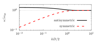
Figure 2: Dispersion relations of the symmetric and antisymmetric surface plasmon-polariton modes of a slab of thickness $D$ consisting of a material described by a Drude model without dissipation, i.e. $\epsilon(\omega)=1-\omega_{\mathrm{p}}^{2}/\omega^{2}$. For $kD/2\gg 1$ both modes merge to the surface plasmon-polariton at $\omega_{\mathrm{sp}}$ for a half-space problem.

The two coupled surface polaritons are labeled symmetric and antisymmetric in relation to the properties of the electric fields they are associated with. Due to the different field distributions within the slab, the symmetric polariton has a lower energy (or frequency) than antisymmetric, with the uncoupled surface polariton’s energy lying in between both. The splitting between of the symmetric and the antisymmetric surface polariton increases as $1/kD$ and it is, therefore, more pronounced for thin slabs, for which the coupling between the surface excitations is stronger. If different dielectric materials were used below and above the slab, additional leaky modes would come into play as elaborated in Ref. Burke1986 . The solutions of Eq. (10) are clearly visible in the imaginary part of the reflection coefficient as shown in Fig. 3, where they are also compared to the resonance of a semi-infinite homogeneous substrate. In Fig. 3 we consider a metal described by the Drude model

$$\epsilon(\omega)=\epsilon^{\infty}-\frac{\omega_{\mathrm{p}}^{2}}{\omega(\omega+i\gamma)},$$ (11)

where $\epsilon^{\infty}>0$ describes the response of the material at large frequencies, $\gamma$ denotes a phenomenological damping constant and $\omega_{\mathrm{p}}$ the plasma frequency. In this case the resonances in the reflection coefficient are associated with the so-called surface plasmon-polaritons. For a bulk-vacuum interface, in the near-field limit, the resonance is located at $\omega_{\rm sp}=\omega_{\rm p}/\sqrt{1+\epsilon^{\infty}}$, while in the case of the slab they depend on the wave-vector and both tend to $\omega_{\rm sp}$ for $kD\to\infty$.

Notice that, in Fig. 3 the behavior at low frequencies (i.e., frequencies much smaller than the resonance frequency) is similar for both the bulk and the slab and describe an ohmic response of both structures. Indeed, in this region, assuming that the material composing the slab or the bulk is ohmic, an expansion of the imaginary part of the reflection coefficient gives

$$r_{I}^{p}(\omega,k)\stackrel{{\scriptstyle\omega\ll\omega_{\mathrm{sp}}}}{{\approx}}\omega\epsilon_{0}\begin{cases}2\rho&\text{for~{}bulk}\\ 2\rho\coth[Dk]&\text{for~{}slab}\end{cases}\,.$$ (12)

Here, $\rho$ represents the material resistivity ($\rho=\gamma/(\epsilon_{0}\omega_{\mathrm{p}}^{2})$ for the Drude model). Notice that, since $k>0$, the imaginary part of the reflection coefficient at low frequencies increases with thinner slabs. In addition, we would have obtained the same result even if the ohmic layer were deposited above a dielectric bulk instead of being suspended in vacuum. These results can be understood in relation to the behavior the symmetric polaritonic resonance, which in case of metals is sometimes called short-range plasmon-polaritons Berini00 ; Berini09 . The field corresponding to the symmetric mode is indeed more confined within the slab material and thus exhibits a stronger dissipative response than both, the single-interface resonance (bulk reflection coefficient) and the anti-symmetric mode (which is sometimes also referred to as the long-range plasmon-polaritons Berini00 ; Berini09 ).

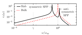
Figure 3: Frequency dependence of the imaginary part of the reflection coefficient in the near-field limit. Two geometries with the same Drude material [Eq. (11)] are considered: A semi-infinite bulk (dotted red line) and a finite slab (solid black line). As parameters we chose typical values for gold (Barchiesi2014, ) $\omega_{\mathrm{p}}=9\,\mathrm{eV}$ and $\gamma=35\,\mathrm{meV}$, $\epsilon_{\mathrm{A}}^{\infty}=1$, a slab thickness of $D=2\,\mathrm{nm}\approx 10^{-3}\,c/\omega_{\mathrm{p}}$ and $k=\omega_{\mathrm{p}}/c$. For the half-space case, a resonance appears at the frequency $\omega_{\rm sp}\approx\omega_{\rm p}/\sqrt{2}$, while for the slab two resonances are visible, one above, the other below $\omega_{\rm sp}$.

For a superlattice structure made by a semi-infinite stack of alternating layers of two different materials (labeled A and B hereafter) with respective thickness $d_{\rm A}$ and $d_{\rm B}$ Albuquerque2004 , the expressions for the reflection coefficients become more involved. To calculate them we need to replace the surface impedance in Eq. (6) with that of the superlattice, $Z_{\mathrm{sup}}^{\sigma}(\omega,k)$. This can be calculated through the transfer matrix formalism Yariv1984 . Within this approach, one propagates the electromagnetic field through each layer and fulfills the boundary conditions at each interface. For instance, the propagation through the layer A is given by

$$\begin{pmatrix}\mathbf{E}\\ c\,\mathbf{B}\end{pmatrix}_{z=z_{0}^{-}+d_{\rm A}}^{\sigma}=\mathbb{M}_{\rm A}^{\sigma}(d_{\rm A})\,\begin{pmatrix}\mathbf{E}\\ c\,\mathbf{B}\end{pmatrix}_{z=z_{0}^{-}}^{\sigma}\,,$$ (13)

where $z_{0}^{-}$ indicates the position directly in front of the interface. The transfer matrix through the local material A reads

$$\mathbb{M}^{\sigma}_{\mathrm{A}}(d_{\rm A})=\begin{pmatrix}\cos(k_{z}^{\mathrm{A}}\,d_{\rm A})&i\delta^{\sigma}\sin(k_{z}^{\mathrm{A}}\,d_{\rm A})\,Z^{\sigma}_{\mathrm{A}}\\ i\delta^{\sigma}\sin(k_{z}^{\mathrm{A}}\,d_{\rm A})/Z^{\sigma}_{\mathrm{A}}&\cos(k_{z}^{\mathrm{A}}\,d_{\rm A})\end{pmatrix}\,.$$ (14)

For non-local materials the transfer matrix takes a different form and explicit expressions can be found in Ref. Intravaia2015 . If we stack the layers A and B we can describe the propagation through the combined block of thickness $d_{\rm sl}=d_{\rm A}+d_{\rm B}$ with the transfer matrix $\mathbb{T}=\mathbb{M}_{\mathrm{B}}\mathbb{M}_{\mathrm{A}}$ or $=\mathbb{M}_{\mathrm{A}}\mathbb{M}_{\mathrm{B}}$, depending on the stacking sequence Kidwai12 . Using the Bloch theorem Bloch1929 for periodic structures, we obtain Mochan1987

$$Z_{\mathrm{sup}}^{\sigma}(\omega,k)=\frac{\mathbb{T}^{\sigma}_{12}}{\exp(i\beta^{\sigma}d_{\rm sl})-\mathbb{T}^{\sigma}_{11}}=\frac{\exp(i\beta^{\sigma}d_{\rm sl})-\mathbb{T}^{\sigma}_{22}}{\mathbb{T}^{\sigma}_{21}}\,.$$ (15)

The Bloch wavevector $\beta^{\sigma}$ can be related to the other parameters of the system through the implicit dispersion relation

$$\cos(\beta d_{\rm sl}) = \cos(k_{z}^{\mathrm{A}}d_{\mathrm{A}})\cos(k_{z}^{\mathrm{B}}d_{\mathrm{B}})-\frac{1}{2}\left(\frac{\epsilon_{\mathrm{A}}k_{z}^{\mathrm{B}}}{\epsilon_{\mathrm{B}}k_{z}^{\mathrm{A}}}+\frac{\epsilon_{\mathrm{B}}k_{z}^{\mathrm{A}}}{\epsilon_{\mathrm{A}}k_{z}^{\mathrm{B}}}\right)$$ (16)

$$\times\sin(k_{z}^{\mathrm{A}}d_{\mathrm{A}})\sin(k_{z}^{\mathrm{B}}d_{\mathrm{B}})\,.$$

Since most of our considerations will address the $p$-polarization (see the discussion above), we drop hereafter the superscript (analogous expressions hold for the $s$-polarization). In addition, we focus on systems composed of alternating conducting and dielectric layers, where the stacking sequence starts with a conducting layer.

Similarly to the coupled surface polaritons found in the slab, an ensemble of excitations linked to the interaction among all the interface modes of the stacking sequences appears in the superlattice system. We refer to this ensemble as collective interface plasmon-polaritons (CIPPs) and their electromagnetic behavior at the vacuum-superlattice interface is, to some extent, similar to that of bulk plasmons occurring in the nonlocal description of metals Camley1984 ; Barton79 ; Note2 .

Indeed, nanostructuring adds to the optical response of the medium certain features which are mathematically reminiscent of spatial nonlocality, although the individual constituents are described in terms of a spatially local permittivity chebykin11 . However, in contrast to bulk plasmons in nonlocal metals, the CIPP fields inside the nanostructured materials are always transverse. In the near-field approximation their dispersion relations are solutions of (see Ref. Camley1984 )

$$\frac{\epsilon_{\mathrm{A}}(\omega)}{\epsilon_{\mathrm{B}}(\omega)}=-C(k,\beta)\pm\sqrt{C^{2}(k,\beta)-1},$$ (17)

where

$$C(k,\beta)=\frac{\cosh(kd_{\mathrm{A}})\cosh(kd_{\mathrm{B}})-\cos(\beta d_{\mathrm{sl}})}{\sinh(kd_{\mathrm{A}})\sinh(kd_{\mathrm{B}})}\,.$$ (18)

Adopting the notation used in Ref. Camley1984 , we write $C(k,\beta)\mp\sqrt{C^{2}(k,\beta)-1}=\exp[\pm\psi(k,\beta)]$. Upon using the Drude model as in Eq. (11) for material A (metal) and a dielectric constant for material B Note3 , the explicit dispersion relation reads

$$\omega_{\pm}(k,\beta)=-\frac{i\gamma}{2}+\sqrt{\frac{\omega_{\mathrm{p}}^{2}}{\epsilon_{\mathrm{A}}^{\infty}+\epsilon_{\mathrm{B}}\exp[\mp\psi(k,\beta)]}-\frac{\gamma^{2}}{4}}\,.$$ (19)

The $\omega_{\pm}$ denote two different branches of possible solutions of Eq. (17). Similar to the result of Eq. (10) for slabs, the two branches can be associated with symmetric ($\omega_{-}$) and antisymmetric ($\omega_{+}$) modes. In fact, depending on the number of supercells, a finite superlattice structure exhibits many distinct symmetric and antisymmetric modes parametrized by discrete values of the Bloch vector Johnson1985 . When the periodic pattern is repeated an infinite number of times, the distinct lines of a finite superlattice structure blur into a continuum Camley1984 (see Fig. 4). Within such a limit, the real part of the Bloch vector $\beta_{R}$ continuously varies within the Brillouin zone $[0,\pi/d_{\rm sl}]$, while the imaginary part $\beta_{I}$ has to be positive in order to obtain a decaying field away from the surface. For non-dissipative material, as a function of the Bloch vector each branch spans two areas on the $(k,\omega)$-plane, which characterize the continua of the symmetric and antisymmetric modes. These areas are bounded by the curves obtained from Eq. (19) for $\beta=0$ and $\beta=\pi/d_{\rm sl}$. Due to damping within the metallic material some of the low frequency modes belonging to the symmetric $\omega_{-}$ branch become overdamped for small wave-vectors. This occurs for the $\omega_{-}$ branch for ($kd_{\mathrm{sl}}\ll 1$; see Fig. 4)

$$k<k_{\mathrm{0}}(\beta)=\frac{\gamma}{\omega_{\mathrm{p}}}\sqrt{\epsilon_{\mathrm{B}}\frac{1-\cos(\beta d_{\rm sl})}{2d_{\mathrm{A}}d_{\mathrm{B}}}}~{}.$$ (20)

In this overdamped region, the modes exhibit a purely imaginary frequency. For example, the lower boundary of the $\omega_{-}$ branch obtained for $\beta=\pi/d_{\rm sl}$ tends to $-\mathrm{i}\gamma$ for $k<k_{\mathrm{0}}(\pi/d_{\rm sl})$. For $\beta=0$, the frequencies is pure imaginary only for $k=0$, indicating that the frequency of the modes near the upper bound of the $\omega_{-}$ branch and the lower bound of the $\omega_{+}$ branch have a nonvashing real part for all wave vectors.

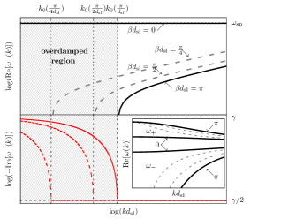
Figure 4: Top panel: Dispersion relation of the $\omega_{-}$ branch on a double logarithmic scale. The thick black solid lines mark the edges of the branch with $\beta d_{\mathrm{sl}}=0,\,\pi$. Some intermediate values for the Bloch vector are also represented (dashed gray lines). The shaded area refers to a region, where the modes become overdamped. For different values of $\beta$, the value of $k_{0}(\beta)$, below which the modes becomes overdamped, varies and shifts to lower $k$ for higher $\beta$. Bottom panel: Negative imaginary part of the $\omega_{-}$ modes. A clearly visible jump occurs for $k\sim k_{0}(\beta)$ and the damping increases from $\gamma/2$ to $\gamma$. Inset: Dispersion relation of the $\omega_{\pm}$ branches, again with the different lines referring to different values of $\beta$, in analogy to the top panel.

Composite nanostructures such as those discussed above are often described through the so-called effective medium approximation (EMA) Bruggeman1935 . This approach relies on the fact that for wavelengths larger than the characteristic geometric length scale of the system (in our case, the thickness of the supercell $d_{\mathrm{sl}}$), the electromagnetic field cannot resolve the details of the system. Instead, the electromagnetic field effectively averages the structural details so that the nanostructures can be described through an effective dielectric function. This approach drastically simplifies the description of complex nanostructures, revealing features which are often obscured by an involved mathematical machinery. Depending on the geometry of the composite system, the resulting effective dielectric function may indeed exhibit properties that are different from those of the constitutive elements. For instance, for our superlattice structures, the EMA describes the system as an uniaxial crystal with a dielectric tensor $\underline{\epsilon}_{\rm EMA}(\omega)=\mathrm{diag}[\epsilon_{\perp}(\omega),\epsilon_{\perp}(\omega),\epsilon_{\parallel}(\omega)]$ whose entries are given by Mochan1987 ; Poddubny13

$$\epsilon_{\perp}(\omega)=\epsilon_{\mathrm{A}}(\omega)\,f+\epsilon_{\mathrm{B}}(\omega)\,(1-f),$$ (21a)

$$\epsilon_{\parallel}(\omega)=\left[\frac{f}{\epsilon_{\mathrm{A}}(\omega)}+\frac{1-f}{\epsilon_{\mathrm{B}}(\omega)}\right]^{-1},$$ (21b)

where $f=d_{\mathrm{A}}/d_{\rm sl}$ gives the filling factor of material A. Equations (21) correspond to the propagation of the electromagnetic field parallel ($\epsilon_{\parallel}$) or orthogonal ($\epsilon_{\perp}$) to the optical axis of the crystal, in our case the $z$-axis. Compared to an isotropic bulk material, in an uniaxial crystal the dielectric response differs along the different principal axes. Specifically, in uniaxial crystals with the optical axis perpendicular to the surface, ordinary waves are associated with the $s$-polarization, whereas extraordinary waves are associated with the $p$-polarization Landau84 . For such systems, the surface impedances are sensitive to the anisotropy and are given by Knoesen1985

$$Z_{\mathrm{EMA}}^{s}(\omega,k)=\frac{\frac{\omega^{2}}{c^{2}}}{\sqrt{\frac{\omega^{2}}{c^{2}}\epsilon_{\perp}(\omega)-k^{2}}}$$ (22a)

$$Z_{\mathrm{EMA}}^{p}(\omega,k)=\frac{\sqrt{\frac{\omega^{2}}{c^{2}}\epsilon_{\parallel}(\omega)-k^{2}}}{\frac{\omega^{2}}{c^{2}}\sqrt{\epsilon_{\perp}(\omega)\epsilon_{\parallel}(\omega)}}.$$ (22b)

In the near-field, the corresponding reflection coefficients take on the form

$$r_{\mathrm{EMA}}^{p}(\omega,k)\approx\frac{\epsilon_{\mathrm{eff}}(\omega)-1}{\epsilon_{\mathrm{eff}}(\omega)+1}\,,\quad r_{\mathrm{EMA}}^{s}(\omega,k)\approx 0,$$ (23)

where we have introduced the effective dielectric function as the geometric mean of the perpendicular and parallel components of the dielectric according to $\epsilon_{\mathrm{eff}}(\omega)=\sqrt{\epsilon_{\parallel}(\omega)\epsilon_{\perp}(\omega)}$.

If we now consider the case where $|\epsilon_{\mathrm{A}}(\omega)|\gg|\epsilon_{\mathrm{B}}(\omega)|$ we can, for a certain frequency range, reduce this effective dielectric function to

$$\epsilon_{\mathrm{eff}}(\omega)\approx\sqrt{\frac{f}{1-f}\epsilon_{\mathrm{A}}(\omega)\epsilon_{\mathrm{B}}(\omega)}=\sqrt{\frac{d_{\rm A}}{d_{\rm B}}\epsilon_{\mathrm{A}}(\omega)\epsilon_{\mathrm{B}}(\omega)}\,.$$ (24)

If in this limit $\epsilon_{\mathrm{B}}>0$ is a constant Note3 , then $\epsilon_{\mathrm{eff}}(\omega)\propto\sqrt{\epsilon_{\mathrm{A}}(\omega)}$. In essence, this yields a criterion when the EMA provides a significant deviation from the ordinary optical response of a bulk system made purely by the material A. To see this more clearly, consider, as an example, an ohmic material which at low frequencies behaves as $\epsilon_{\mathrm{A}}(\omega)\approx\mathrm{i}(\omega\epsilon_{0}\rho)^{-1}$ (e.g., a Drude metal for $\omega<\gamma$). Within the effective medium description, for the reflection coefficient we then have

$$r_{I}(\omega,k)\approx\sqrt{\omega\epsilon_{0}}\sqrt{2\frac{\rho}{\epsilon_{\mathrm{B}}}\frac{d_{\rm B}}{d_{\rm A}}}.$$ (25)

Therefore in the case of a metal-dielectric superlattice structure, the EMA predicts that for $\omega<\gamma$ the behavior of the reflection coefficient is no longer ohmic but sub-ohmic.

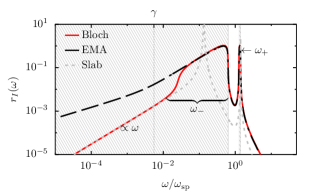
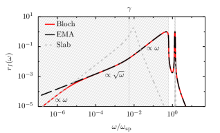
Figure 5: Limiting behavior of the superlattice’s reflection coefficient ($p$-polarization) versus the full calculation. The imaginary part of the reflection coefficient is plotted as a function of $\omega$. The conducting material’s dielectric function, $\epsilon_{\rm A}(\omega)$, is described by a Drude model with the same parameters as in Fig. 3. The dielectric is vacuum ($\epsilon_{\rm B}=1$), while the filling factor and the wave-vector are set to $f=0.2$ and $k=10^{-1}c/\omega_{\mathrm{p}}$. The full tranfer-matrix-based calculation exhibits features which can be directly connected to the continuum of modes in the $\omega_{\pm}$-branches. For frequencies $\omega$ higher than the lower bound of the $\omega_{-}$-branch, the EMA calculation (dashed black line) shows a very good agreement with the transfer-matrix approach (solid red line). At small frequencies $\omega$, the full transfer-matrix calculation is equivalent to the behavior of the very first conducting layer of the structure (gray dotted line). The shaded areas represent the hyperbolic regime with $\mathrm{Re}\left\{\epsilon_{\perp}(\omega)\right\}\mathrm{Re}\left\{\epsilon_{\parallel}(\omega)\right\}<0$.

Figure 6: Analogous comparison as in Fig. 6 but this time for $k=10^{-3}c/\omega_{\mathrm{p}}$. The EMA holds over a larger frequency range and for lower frequencies $\omega$. A sub-ohmic behavior ($r_{\mathrm{I}}\propto\sqrt{\omega}$) is visible in the Bloch-wave calculations. At low frequencies, the EMA breaks down and effectively only the first slab is responsible for the scattering properties of the entire structure.

Figures 6 and 6 display the above features and certain structures related to the CIPP modes. Using the different approaches described above (Bloch waves and EMA), both plots display the frequency dependence $r^{p}_{I}(\omega,k)$ for two distinct values of the wave-vector, one above and one below the value $k_{\mathrm{0}}(\pi/d_{\rm sl})$ that delineates the overdamped region. Notice that the EMA agrees with the full calculation only above a certain frequency. The breakdown of the approximation occurs for frequencies around the lower boundary of the $\omega_{-}$ branch. This can be understood by recalling that in this region $\beta d_{\mathrm{sl}}\approx\pi$ (see Fig. 4), while previous work Mochan1987 has shown that the expressions in Eqs. (21) are only compatible with $\beta d_{\mathrm{sl}}\ll 1$. In both plots, we can see that for $\omega<\gamma$ the EMA description enters the sub-ohmic regime discussed above. This behavior is also featured by the full calculation as long as $\gamma$ lies above the lower boundary of the $\omega_{-}$ branch. Indeed, in Fig. 6, due to the choice of the wave-vector, the $\omega_{-}$ branch is stretched to lower frequencies $\omega$ and the lower bound is not marked by a distinct edge as that appearing in Fig. 6. The sub-ohmic feature of the superlattice occurs in the region where the modes of the $\omega_{-}$ branch becomes overdamped, connecting it to the collective low frequency behavior of the (non-resonant) CIPP. Conversely, the shoulder appearing in Fig. 6 can be interpreted as resulting from the coalescence of all the (infinite) CIPP resonances occurring in the semi-infinite superlattice.

The EMA also provides the framework for another interesting aspect of superlattice structures (or in general uniaxial crystals), namely the appearance of hyperbolic dispersions Poddubny13 . Indeed, depending on the sign of $\mathrm{Re}\{\epsilon_{\parallel,\perp}\}$, isofrequency surfaces in the 3D-wavevector space can be either ellipsoids or hyperboloids. The latter occurs when $\mathrm{Re}\{\epsilon_{\parallel}\}\mathrm{Re}\{\epsilon_{\perp}\}<0$ and, depending on which of the permittivities is negative, one distinguishes between hyperbolic material of type I ($\mathrm{Re}\{\epsilon_{\parallel}\}<0$ and $\mathrm{Re}\{\epsilon_{\perp}\}>0$) or of type II ($\mathrm{Re}\{\epsilon_{\parallel}\}>0$ and $\mathrm{Re}\{\epsilon_{\perp}\}<0$). Distinct from a usual dispersion, in hyperbolic materials a large number of wavevectors can be connected with a narrow range of frequencies leading to a significant increase in the system’s density of states Poddubny13 . In Fig. 6 and 6 the shaded areas indicate where our superlattice behaves as a hyperbolic material. For a metal, modeled by a Drude model, with low damping ($\gamma\ll\omega_{\mathrm{p}}$) and a dielectric with constant $\epsilon_{\rm B}>0$, the frequencies where the relative sign flips are given by

$$\omega_{\mathrm{h1}}\sim\omega_{\mathrm{p}}\sqrt{\frac{f}{f\epsilon_{\mathrm{A}}^{\infty}+(1-f)\epsilon_{\mathrm{B}}}},$$ (26a)

$$\omega_{\mathrm{h2}}\sim\omega_{\mathrm{p}}\sqrt{\frac{1-f}{f\epsilon_{\mathrm{B}}+(1-f)\epsilon_{\mathrm{A}}^{\infty}}},\quad\omega_{\mathrm{h3}}\sim\frac{\omega_{\mathrm{p}}}{\sqrt{\epsilon_{\mathrm{A}}^{\infty}}}\,.$$ (26b)

We notice that, under the condition of validity of the EMA, this behavior is essentially related with the location of the $\omega_{\pm}$-branches, establishing a direct connection with the CIPP Isic2017 . Interestingly, this offers another perspective on the features we observe in $r_{I}(\omega)$. Indeed, if we exclude the sub-ohmic region, where the material dissipation is relevant, the shoulders appearing in the plots (in particular in Fig. 6) can be seen as a manifestation of the hyperbolic behavior of the semi-infinite superlattice. In fact, due to the change in sign of the permittivities, in this region $\mathrm{Im}\{\epsilon_{\mathrm{eff}}(\omega)\}$ and therefore $r_{I}(\omega)$ can be substantially different from zero even for a vanishingly small material damping. This additional loss channel can be understood by the deep penetration of the CIPPs, which allows to accumulate even very small losses throughout the whole semi-infinite superlattice substrate.

The above plots also highlight the relevance of the wavevector regarding the validity of the EMA, showing that the smaller the value of $k$ (near to orthogonal incidence) becomes, the better is the quality of the EMA. Importantly, both Figs. 6 and 6 reveal that at low frequencies, below the area described by the $\omega_{-}$ branch of the CIPP, the EMA description ceases to be valid. In this case, the optical response of the superlattice structure essentially reduces to that of the first metallic layer in the system, recovering the ohmic behavior of a single slab. Physically, this can be understood as the result of a shorter penetration of the field into the structure: The EMA breaks down for penetration depths which are shorter than the thickness of the supercell (the field is no longer able to resolve deeper lying layers).

This is also visible in Fig. 7 where the wavevector dependence of the reflection coefficient $r^{p}_{I}(\omega,k)$ is depicted for a fixed frequency: For small wavevectors, the full result is indeed well represented by the EMA, while for large wavevectors we recover the slab’s reflection coefficient. When this occurs, the transition between the ohmic and the sub-ohmic behavior is characterized by the wavevector $k_{t}(\omega)$, which for small frequencies can be written as

$$k_{t}\approx\sqrt{\omega\epsilon_{0}}\sqrt{\frac{2\rho\epsilon_{\rm B}}{d_{\rm A}d_{\rm B}}}~{},$$ (27)

and can be obtained by comparing the results in Eqs. (12) and (25). For $k<k_{t}$ the superlattice is well described by the reflection coefficient provided by the EMA, while for $k>k_{t}$ the slab description and eventually the bulk description for $k>1/d_{\rm A}$.

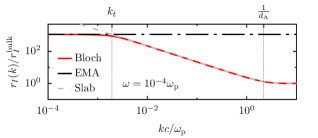
Figure 7: Wavevector dependence of the imaginary part of the $p$-polarized reflection coefficient for $\omega=\sqrt{2}\times 10^{-4}\omega_{\rm sp}$. The material parameters were chosen analogous to Fig. 3 with $d_{\mathrm{A}}=d_{\mathrm{B}}=10\,\mathrm{nm}$ ($\sim 6\times 10^{-3}\,c/\omega_{\mathrm{p}}$). The results for the full Bloch-wave calculation (red line), the EMA (black dash-dotted line) and the slab description (dashed gray line) are normalized by the imaginary part of the reflection coefficient for a metallic half-space. The full calculation is well described by the EMA at low $k$ (near orthogonal incidence) and it recovers the slab and the bulk results for $k>k_{t}$ and $k>1/d_{\rm A}$, respectively.

IV Quantum friction with superlattice structures

The analyses presented in the previous sections allow for a quantitative assessment of quantum friction as well as for a deeper qualitative understanding of the behavior of the force in systems involving semi-infinite superlattice substrates. Even if most of the following analytical expressions rely on the near-field approximation, the numerical calculations consider the entire retarded interaction and are thus exact. For the conducting layer, in addition to the Drude model in Eq. (11) with the parameters used to describe gold ($\omega_{\mathrm{p}}=9\,\mathrm{eV}$, $\epsilon^{\infty}=5$ and $\gamma=1.1\times 10^{-5}\omega_{\mathrm{p}}$ Pirozhenko2008a ), we also consider doped silicon

$$\epsilon_{\mathrm{dop}}(\omega) = \epsilon_{\mathrm{Si}}(\omega)-\frac{\omega_{\mathrm{pSi}}^{2}}{\omega(\omega+i\gamma_{\mathrm{Si}})}\,.$$ (28)

In the previous model, the free charge carries are described by an additional Drude term, while the intrinsic permittivity of silicon is given by

$$\epsilon_{\mathrm{Si}}(\omega)=\epsilon_{\mathrm{Si}}^{\infty}-\frac{(\epsilon^{0}_{\mathrm{Si}}-\epsilon_{\mathrm{Si}}^{\infty})\omega_{0}^{2}}{\omega^{2}-\omega_{0}^{2}}$$ (29)

with $\epsilon_{\mathrm{Si}}^{\infty}=1.035$, $\epsilon^{0}_{\mathrm{Si}}=11.87$ and $\omega_{0}\approx 4.34\,\mathrm{eV}$ Bergstroem1997 . Due to the variability of the doping, we gain access to a wide range of values for the resistivity, $\rho_{\rm dSi}=\gamma_{\mathrm{Si}}/(\epsilon_{0}\omega_{\mathrm{pSi}}^{2})$, while maintaining the same basic material description. The dielectric material B is instead chosen to be intrinsic silicon or, for simplicity, vacuum (i.e. $\epsilon_{\mathrm{B}}=1$). From the expression presented in the previous section we expect that the value of dielectric function for this layer mostly produces a shift or a rescaling of the features induced by the conducting material (see for example Eqs. (19) and (25) as well as Fig. 9 and the expression below).

Let us start our analysis by focusing on the non-resonant regime, where the force is essentially connected to wavevectors $k\lesssim 1/z_{a}$ and frequencies $0<\omega\lesssim v/z_{a}$. In Sec. III we have shown that, depending on the frequencies and the wavevectors, the optical response of superlattice structures effectively changes, featuring behavior typical of a homogeneous bulk, a thin slab or, using the EMA description, an uniaxial crystal. Similarly we can expect that, as a function of the atom’s velocity and distance from the surface, the quantum frictional force explores all the previously discussed regimes.

At very low velocities and very short distances, despite the fact that a wide range of frequencies can participate in the interaction, from the point of view of quantum friction the semi-infinite superlattice behaves as an ohmic medium, indicating a force which is proportional to $v^{3}$. The analysis of the previous section, suggests indeed that, as long as $k_{t}z_{a}\ll 1$, the superlattice is equivalent to a metallic bulk or at most a metallic slab. In fact, in agreement with the behavior depicted in Fig. 7, for $z_{a}\ll d_{\rm A}$ we recover the expression for the force acting on an atom moving above a homogeneous substrate composed of an ohmic material Intravaia2016a

$$\bar{F}\sim\bar{F}_{\mathrm{bulk}} \stackrel{{\scriptstyle v\ll c}}{{\approx}} -\frac{864}{5\pi^{3}}\hbar\alpha_{0}^{2}\rho^{2}\frac{v^{3}}{(2z_{a})^{10}}\,.$$ (30)

As explained above, the $v^{3}$-scaling is rooted in the linear-in-frequency (ohmic) behavior of the imaginary part of reflection coefficient at small frequencies $\omega$ (see Fig. 6). The $z_{a}^{-10}$ dependence results, instead, from a combined dependence on $k$ and $\omega$ of the total Green tensor. For ohmic materials the proportionality to the square of resistivity $\rho$ can be directly understood from the functional behavior of Eq. (4). In Eq. (30) and in all subsequent analytical expressions the bar (e.g. $\bar{F}$) indicates the average over all dipole angles. For simplifying the evaluation, however, our numerical analysis considers the case $\mathbf{d}=\sqrt{\alpha_{0}/3}\,(1,1,1)$, where $\alpha_{0}=\mathrm{Tr}[\underline{\alpha}_{0}/3]$.

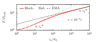
Figure 8: Quantum frictional force on an atom moving above a superlattice (red solid line) as a function of the atom-surface separation. The force is normalized to the bulk result [Eq. (30)]. At large separations, the superlattice can be approximated by an EMA description (dotted black line) which yields a $z_{a}^{-9}$ law. At small distances, instead, the superlattice can essentially be replaced by the top-most (conducting) layer (gray dashed line). The result for a metallic slab features the transition to bulk behavior, $z_{a}^{-8}\to z_{a}^{-10}$ occurring as soon as $z_{a}\ll d_{\rm A}$. As material parameters we used doped silicon with $\omega_{\mathrm{pSi}}=0.0725\,\mathrm{eV}$, $\gamma_{\mathrm{Si}}=0.0247\,\mathrm{eV}$ and $d_{\mathrm{A}}=d_{\mathrm{B}}=1\,\mathrm{nm}$ ($\sim 7\times 10^{-12}\,c/\omega_{\mathrm{pSi}}$).

When the distance increases, keeping the low velocity limit, the optical response is still ohmic at low frequencies but with a resistivity that effectively increases according to Eq. (12). In this regime, despite the fact that the force still remains proportional to $v^{3}$, the semi-infinite superlattice is effectively represented by its first layer and its thickness, $d_{\rm A}$, appears as an additional length scale of the system. This modifies the functional dependence of quantum friction on the atom-surface separation and for $z_{a}\gtrsim d_{\rm A}$ we obtain

$$\bar{F}\sim\bar{F}_{\mathrm{slab}}\approx\bar{F}_{\mathrm{bulk}}\mathcal{C}_{\mathrm{slab}}(z_{a}/d_{\rm A}).$$ (31)

The monotonous and positive function $\mathcal{C}_{\mathrm{slab}}(x)$, whose explicit form is given in Appendix A, is such that $\mathcal{C}_{\mathrm{slab}}(x\to 0)=1$, recovering the limit of Eq. (30), and $\mathcal{C}^{\mathrm{slab}}(x\gg 1)\propto x^{2}$. Importantly, Eq. (31) scales as $z_{a}^{-8}$ for $z_{a}\gtrsim d_{\rm A}$. Therefore the force decays slower with $z_{a}$ than in Eq. (30), leading to an enhancement of several orders of magnitude with respect to the bulk result (see Fig. 8). In simple terms, this geometry-induced modification and the corresponding increase in the value of the force can be understood as a consequence of the fact that, while the intrinsic resistivity of the material is constant, the layer’s resistance effectively increases as its thickness is reduced.

With a further increase in the atom-surface separation, the changes in the behavior of the quantum frictional force acting on an atom moving at constant velocity above the semi-infinite superlattice become more profound, as the interaction starts to “perceive” the substrate as being well-described by the EMA. According to Eq. (27), in the non-resonant regime we roughly expect such change of behavior to occur when

$$vz_{a}\gtrsim\frac{d_{\rm A}d_{\rm B}}{2\rho\epsilon_{0}\epsilon_{\rm B}},$$ (32)

which also indicates the necessity of sufficiently large velocities (for $v\to 0$ the recover the ohmic behavior). In this region we have that

$$\bar{F}\sim\bar{F}_{\mathrm{EMA}}\approx-\hbar\alpha_{0}^{2}\frac{6\rho}{\pi^{2}\epsilon_{0}\epsilon_{\mathrm{B}}}\frac{d_{\rm B}}{d_{\rm A}}\frac{v|v|}{(2z_{a})^{9}}.$$ (33)

We first notice that the force no longer grows quadratically but linearly with the resistivity of the material. The effective sub-ohmic description introduced by the EMA does not only lead to a change in the velocity-dependence of the force ($v^{3}\to v^{2}$, as discussed in Sec. II), but also to an additional modification of its functional dependence on the atom-surface separation.

Figure 8 depicts the quantum frictional force for fixed velocity as a function of the atom-surface separation $z_{a}$. We observe that with the superlattice structuring, we access the three different regimes discussed above: At short distances, we recover the bulk expression $F\propto z_{a}^{-10}$ given in Eq. (30); for intermediate separations ($z_{a}\gtrsim d_{\rm A}$, the slab regime where $F\propto z_{a}^{-8}$ occurs; finally, for sufficiently large separations, the EMA regime is reached, yielding $F\propto z_{a}^{-9}$.

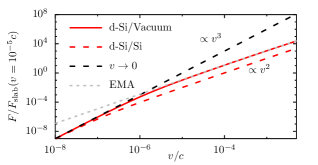
Figure 9: Velocity dependence of the quantum frictional force, normalized to the value of the slab configuration at $v=10^{-5}\,c$. The atom moves above a superlattice with doped-silicon as conducting layer and intrinsic silicon (solid red line) [see Eq. (29)] or vacuum (dashed red line) as dielectric layer. The distance is fixed at $z_{a}\approx 70\,c/\omega_{\mathrm{p}}^{\mathrm{Si}}$ ($\sim 1\mu$m for the materials considered). The other parameters are the same of in Fig. 8. In both cases, the full calculations via the Bloch-wave approach features a transition from $v^{3}$ behavior at low velocities (dashed black line), typical of ohmic materials, to the $v^{2}$ dependence characteristic of the sub-ohmic behavior ($r_{I}\propto\sqrt{\omega}$) of the EMA (dotted gray line).

The velocity dependence of the quantum frictional force is presented in Fig. 9. At sufficiently low velocities, we recover the $v^{3}$ law, which is connected to ohmic response of the superlattice and this essentially originates from its first layer. However, for increasing velocities a broader range of frequencies contributes to the interaction and eventually the region where the structure changes its behavior from ohmic to sub-ohmic becomes relevant. This corresponds to a change of the velocity dependence of the force from $v^{3}$ to $v^{2}$. Finally, it is interesting to consider the characteristic of the resonant contribution to quantum friction in systems involving semi-infinite superlattices. As described in Sec. III and shown in Fig. 6, for certain parameters we observe large values of $r_{I}$ due to the coalescence of the resonances occurring in the $\omega_{\pm}$ branches. This behavior, which is connected with the hyperbolic dispersion of the structure, is particularly evident for a superlattice composed of low-damping materials, where the sub-ohmic regime is less pronounced. For these frequencies, even if the material has very weak dissipation, the continuum of modes in the $\omega_{-}$ branch (and similarly but at higher frequencies for the $\omega_{+}$ branch) effectively behaves as an “energy sink” which, through a non-radiative coupling with the atom, can efficiently transport energy away from the surface through the superlattice. Depending on the velocity and the distance of the atom, this frequency region can give rise to a resonant contribution, which leads to an additional increase of the force. The interaction generating the CIPP also shifts this frequency range to a frequency below $\omega_{\rm sp}$, lowering the corresponding resonant velocity threshold and adding a certain degree of tunability via the thickness of the layers. In Fig. 10, we indeed observe a steady increase of the quantum frictional force that occurs at a relatively low velocity. Due to the broadband nature of the $\omega_{-}$ band, this resonant contribution differs from that generated by an isolated resonance (see for example Refs. Intravaia2016 ; Intravaia2016a ) and the system features a smoother transition out of the non-resonant regime.

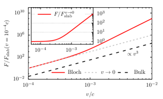
Figure 10: Resonant enhancement of quantum friction due to the CIPP modes. The quantum frictional force acting on an atom moving above superlattice structures is enhanced due to the interaction with the coalescence of the CIPP resonances in the $\omega_{-}$ branch [Eq. (19)]. In order to clearly reveal the effect of CIPP modes, we have chosen a large atomic transition frequency ($\omega_{a}=10.2\,\mathrm{eV}$, as e.g. for hydrogen) and a Drude metal with low damping constant $\gamma=1.1\times 10^{-5}\omega_{\mathrm{p}}$ with $\omega_{\mathrm{p}}=9\,\mathrm{eV}$ (further parameters are $\epsilon_{\mathrm{A}}^{\infty}=5$, $d_{\mathrm{A}}=d_{\mathrm{B}}=1\,\mathrm{nm}$ and $z_{a}=10\,\mathrm{nm}$). For comparison, in addition to the full Bloch-wave calculations (red solid line), the plot shows the asymptote for small velocities (grey dotted line) and the calculations for a Drude bulk substrate (dashed black line). The offset for low velocities between the bulk substrate and the superlattice results can be understood by the different $z_{a}$ dependence as displayed in Fig. 8. Inset: The full Bloch-wave calculation is normalized by its low-velocity limit, which coincides with the result of the slab configuration.

V Conclusions

Modern technologies allow for the structuring of materials at the size of nanometers, prompting novel applications in several areas of physics. In this work, we have shown that such nanostructuring can be very interesting with regards to nonequilibrium atom-surface interactions and in particular for controlling the strength and the functional dependencies of the quantum frictional force on an atom moving at constant velocity and height above multi-layered structures. Indeed, when these structures consist of a semi-infinite superlattice of alternating metallic and dielectric layers, the spectrum of vacuum fluctuations is considerably modified relative to that of an homogeneous medium and can be tuned by changing the thickness and the material properties of the layers. In these systems, the frequency spectrum is characterized by the appearance of coupled interface plasmon-polariton (CIPP) modes: They arise from the electromagnetic interaction among the charge-carrier densities existing at the metal-dielectric interfaces and can be considered as the generalization of the surface plasmon-polariton resonances appearing at metallic surfaces. Mathematically, for semi-infinite superlattices, the CIPP modes manifest themselves as two continua characterized by well-prescribed symmetries of the associated electromagnetic field. Their behavior is also connected with the properties of the superlattice to exhibit hyperbolic dispersions. We have seen that CIPP modes affect the quantum frictional forces in different ways depending on the speed of the atom and on its distance from the surface. At low velocity, the force is strongly connected with the low-frequency behavior of the surface’s $p$-polarized reflection coefficient, $r^{p}(\omega,k)$. In superlattices, depending on the wavevector, we have observed a change in behavior of the imaginary part of the reflection coefficient, from ohmic ($r^{p}_{I}\propto\omega$) to sub-ohmic ($r^{p}_{I}\propto\sqrt{\omega}$). The former can be ascribed to the electromagnetic response of the first metallic layer in the stacking sequence, while the latter is related to an overdamped (non-resonant) subset of the CIPP modes. We have shown that, for the quantum frictional force, this behavior can lead to enhancements of several orders of magnitude relative to the case of a homogeneous bulk substrate, as well as to a modification of the power law describing its functional dependence on the atom-surface separation ($z_{a}^{-10}\to z_{a}^{-8}\to z_{a}^{-9}$, see Fig. 8). Similarly, the velocity dependence changes from $\propto v^{3}$, typical of the ohmic response, to $\propto v^{2}$ induced by $r^{p}_{I}\propto\sqrt{\omega}$ (see Fig. 9). The threshold distances and velocities, where these transitions take place, depend on the material properties and geometrical parameters of the system [Eq. (32)]. Finally, at higher velocities resonant phenomena can become important. An analysis of the relevant expressions shows that the velocity threshold, when this occurs, is usually rather high due to the large typical values of the involved resonance frequencies. However, we have shown that in superlattice systems, by reducing the layers’ thickness, the interaction among all the surface plasmon polaritons at the different material interfaces lead to a displacement of the continuum of CIPP resonances to lower energy, allowing for a more accessible resonant enhancement of the quantum frictional force (see Fig. 10). This behavior has been further connected with the hyperbolic properties of the semi-infinite superlattice. Indeed even for low dissipative materials, the increase in the density of states connected with the hyperbolic dispersion creates an additional channel through which energy can be carried deep into the substrate.

These results highlight once more the role of geometry and material properties in fluctuation-induced phenomena and indicate a pathway for future experimental investigations of nonequilibrium atom-surface effects. While the geometry can be used to control (enhance or suppress) the interaction by changing the functional dependence of the quantum frictional force, the material properties offer a direct access to the proportionality constants. As an example, using high-resistivity materials such as GaAs ($\rho_{\mathrm{GaAs}}\approx 10^{9}\,\Omega\mathrm{cm}$) in a superlattice structure (vacuum as a dielectric, for simplicity) with $10\,\mathrm{nm}$ thick layers, our analysis predicts a quantum friction force of $F\approx-15\,\mathrm{fN}$ acting on a ${}^{87}\mathrm{Rb}$ atom moving at a height of $z_{a}=0.1\,\mathrm{\mu m}$ above the multi-layer surface with a velocity of $v=5\times 10^{-4}c$. This value of the quantum frictional force corresponds to an acceleration of about $10^{11}\mathrm{m/s^{2}}$ which is within the presently available experimentally measurable accuracy. An experimental confirmation of quantum frictional forces would be of high fundamental interest and can provide a deeper understanding of the underlying physics of nonequilibrium quantum-fluctuation-induced phenomena.

Appendix A Definitions and low-velocity limit

The definition of the quantum frictional force essentially depends on two susceptibilities, the atomic polarizability, characterizing the moving microscopic object, and the Green tensor that characterizes the electromagnetic properties of the nanostructured substrate. In general, the Green tensor can be written as the sum of the vacuum contribution $\underline{G}_{0}$ and a scattered contribution $\underline{g}$. While the expression for the former can be found in textbooks (see for example Ref. Jackson75 ), for flat surfaces $\underline{g}$ the latter takes the form Wylie1984

$$\underline{g}(\mathbf{k},z_{a},\omega)=\frac{e^{-2\kappa z_{a}}\kappa}{2\epsilon_{0}}\left[r^{p}(\omega,k)\mathbf{p}_{+}\mathbf{p}_{-}+\frac{\omega^{2}}{c^{2}\kappa^{2}}r^{s}(\omega,k)\mathbf{s}\mathbf{s}\right]~{},$$ (34)

Here, we have introduced $\kappa=\sqrt{k^{2}-\omega^{2}/c^{2}}$ ($\mathrm{Re\{\kappa\}>0}$ and $\mathrm{Im\{\kappa\}<0}$). Further, $k^{2}=k_{x}^{2}+k_{y}^{2}$ and $r^{\sigma}$ are the reflection coefficients for the two polarizations, $\sigma=s,p$, and

$$\mathbf{s}=\frac{\mathbf{k}}{k}\times\frac{\mathbf{z}}{z},\quad\mathbf{p}_{\pm}=\frac{k}{\kappa}\frac{\mathbf{z}}{z}\mp i\frac{\mathbf{k}}{k}\,.$$ (35)

In these expressions, $\mathbf{z}$ represents the vector in $z$ direction (perpendicular to the surface of the substrate). In terms of the Green tensor we can also define the velocity-dependent polarizability tensor

$$\underline{\alpha}(\omega,\mathbf{v}) = \frac{\underline{\alpha}_{0}\omega_{a}^{2}}{\omega_{a}^{2}-\omega^{2}-\Delta_{a}(\omega;\mathbf{v})-i\omega\gamma_{a}(\omega;\mathbf{v})},$$ (36)

where the dyadic $\underline{\alpha}_{0}=\mathbf{d}\mathbf{d}$ is the static polarizability and have introduced the abbreviations

$$\Delta_{a}(\omega)=\omega_{a}^{2}\int\frac{\mathrm{d}^{2}\mathbf{k}}{(2\pi)^{2}}\,\mathrm{Tr}\left[\underline{\alpha}_{0}\cdot\underline{G}_{R}(\mathbf{k},z_{a},\omega+\mathbf{k}\cdot\mathbf{v})\right],$$ (37a)

and

$$\gamma_{a}(\omega)=\frac{\omega_{a}^{2}}{\omega}\int\frac{\mathrm{d}^{2}\mathbf{k}}{(2\pi)^{2}}\,\mathrm{Tr}\left[\underline{\alpha}_{0}\cdot\underline{G}_{I}(\mathbf{k},z_{a},\omega+\mathbf{k}\cdot\mathbf{v})\right]$$ (37b)

which, respectively, describe the induced frequency shift and damping. The polarizability also appears in the expression of the nonequilibrium correction to the fluctuation-dissipation theorem

$$\underline{J}(\omega;\mathbf{v}) = \int\frac{\mathrm{d}^{2}\mathbf{k}}{(2\pi)^{2}}\left[\theta(\omega+\mathbf{k}\cdot\mathbf{v})-\theta(\omega)\right]$$

$$\times\,\underline{\alpha}(\omega;\mathbf{v})\cdot\underline{G}_{I}(\mathbf{k},z_{a},\omega+\mathbf{k}\cdot\mathbf{v})\cdot\underline{\alpha}^{*}(\omega;\mathbf{v})$$

which occurs in Eq. (3).

Altogether, the above expressions allow the evaluation of the non-relativistic value of the quantum frictional force given in Eq. (1). The structure of Eq. (3) indicates that the quantum friction force can be decomposed into a contribution related to the local thermal equilibrium (LTE) approximation and a full nonequilibrium correction. This separation is also visible in low velocity approximation of the force given in Eq. (4), where the first term on the r.h.s. is the result within the LTE, $F^{\mathrm{LTE}}$, while the second, $F^{J}$, is entirely due to the the tensor $\underline{J}(\omega;\mathbf{v})$.

Equation (4) also shows that the low-velocity behavior of the force is connected to the low-frequency features of the nano-structures optical response and eventually with the low-frequency expansion of the imaginary part of the reflection coefficients. We have seen in the main text that for metal-dielectric superlattice structures, at sufficiently small atom-surface separations, the optical response is dominated by the first (metallic) layer. Effectively, the quantum frictional force felt by the atom is the same as that produced by a metallic slab, i.e., $F_{\mathrm{sup}}\approx F_{\mathrm{slab}}$. Using the expressions in Eq. (12) this allows for the following estimates. For the LTE term, we obtain

$$\frac{F^{\mathrm{LTE}}_{\mathrm{slab}}}{F_{\mathrm{bulk}}^{\mathrm{LTE}}}=\mathcal{C}^{\mathrm{LTE}}_{\mathrm{slab}}(\tfrac{z_{a}}{D})\\ \stackrel{{\scriptstyle v\rightarrow 0}}{{\approx}}\frac{\int_{0}^{\infty}\mathrm{d}k\,k^{6}e^{-2kz_{a}}\coth(kD)}{\int_{0}^{\infty}\mathrm{d}k\,k^{6}e^{-2kz_{a}}}\\ \times\frac{\int_{0}^{\infty}\mathrm{d}k\,k^{2}e^{-2kz_{a}}\coth(kD)}{\int_{0}^{\infty}\mathrm{d}k\,k^{6}e^{-2kz_{a}}}$$ (39)

where $F_{\mathrm{bulk}}^{\mathrm{LTE}}$ is the LTE contribution to the quantum frictional force in the case of a homogeneous semi-infinite substrate. Its value

$$\bar{F}_{\mathrm{bulk}}^{\mathrm{LTE}}\approx-\frac{21}{20}\frac{90}{\pi^{3}}\hbar\alpha_{0}^{2}\rho^{2}\frac{v^{3}}{(2z_{a})^{10}}$$ (40)

has already ben calculated in Ref. Intravaia2016a , where the bar indicates the average over the dipole angles. The function that gives the correction induced by the finite thickness is defined as

$$\mathcal{C}_{\mathrm{slab}}^{\mathrm{LTE}}(\tfrac{z_{a}}{D})=\left[1-2\frac{\zeta\left(7,\frac{z_{a}}{D}\right)}{(D/z_{a})^{7}}\right]\left[1-2\frac{\zeta\left(3,\frac{z_{a}}{D}\right)}{(D/z_{a})^{3}}\right]\,,$$ (41)

where

$$\zeta(s,x)=\sum_{n=0}^{\infty}\frac{1}{(n+x)^{s}}$$ (42)

is the Hurwitz Zeta function. Upon applying the same strategy to the nonequilibrium contribution we obtain an analogous expression that reads as

$$\bar{F}_{\mathrm{bulk}}^{J}\approx-\frac{87}{80}\frac{72}{\pi^{3}}\hbar\alpha_{0}^{2}\rho^{2}\frac{v^{3}}{(2z_{a})^{10}}$$ (43)

and the corresponding correction function

$$\mathcal{C}_{\mathrm{slab}}^{J}(\tfrac{z_{a}}{D})=\left[1-2\frac{\zeta\left(5,\frac{z_{a}}{D}\right)}{(D/z_{a})^{5}}\right]^{2}\,.$$ (44)

Adding the two contributions, we can define the total correction function introduced in Eq. (31)

$$\mathcal{C}_{\mathrm{slab}}(\tfrac{z_{a}}{D})=\frac{F^{\mathrm{LTE}}_{\mathrm{bulk}}\mathcal{C}_{\mathrm{slab}}^{\mathrm{LTE}}(\tfrac{z_{a}}{D})+F^{J}_{\mathrm{bulk}}\mathcal{C}_{\mathrm{slab}}^{J}(\tfrac{z_{a}}{D})}{F^{\mathrm{LTE}}_{\mathrm{bulk}}+F^{J}_{\mathrm{bulk}}},$$ (45)

which clearly inherits the properties of the functions defined above. For $z_{a}\gg D$ we have that

$$\bar{F} \approx\bar{F}_{\mathrm{slab}}\approx\stackrel{{\scriptstyle z_{a}\gg D}}{{\approx}}-\frac{\hbar\alpha_{0}^{2}\rho^{2}}{D^{2}\pi^{3}}\frac{v^{3}}{(2z_{a})^{8}}\frac{2043}{160}.$$ (46)

References

- (1) H. B. G. Casimir and D. Polder, The Influence of Retardation on the London-van der Waals Forces, Phys. Rev. 73, 360 (1948).
- (2) F. Intravaia, R. O. Behunin, C. Henkel, K. Busch, and D. A. R. Dalvit, Non-Markovianity in atom-surface dispersion forces, Phys. Rev. A 94, 042114 (2016).
- (3) F. Intravaia, V. E. Mkrtchian, S. Y. Buhmann, S. Scheel, D. A. R. Dalvit, and C. Henkel, Friction forces on atoms after acceleration, J. Phys. Condens. Matter 27, 214020 (2015).
- (4) G. Pieplow and C. Henkel, Cherenkov friction on a neutral particle moving parallel to a dielectric, J. Phys. Condens. Matter 27, 214001 (2015).
- (5) G. Dedkov and A. Kyasov, Electromagnetic and fluctuation-electromagnetic forces of interaction of moving particles and nanoprobes with surfaces: A nonrelativistic consideration, Phys. Solid State 44, 1809 (2002).
- (6) S. Scheel and S. Y. Buhmann, Casimir-Polder forces on moving atoms, Phys. Rev. A 80, 042902 (2009).
- (7) W. Yan, M. Wubs, and N. A. Mortensen, Hyperbolic metamaterials: Nonlocal response regularizes broadband supersingularity, Phys. Rev. B 86, 205429 (2012).
- (8) Z. Liu, H. Lee, Y. Xiong, C. Sun, and X. Zhang, Far-Field Optical Hyperlens Magnifying Sub-Diffraction-Limited Objects, Science 315, 1686 (2007).
- (9) P. Shekhar, J. Atkinson, and Z. Jacob, Hyperbolic metamaterials: fundamentals and applications, Nano Convergence 1, 1 (2014).
- (10) A. W. Rodriguez, F. Capasso, and S. G. Johnson, The Casimir effect in microstructured geometries, Nat. Photon. 5, 211 (2011).
- (11) F. Intravaia, P. S. Davids, R. S. Decca, V. A. Aksyuk, D. López, and D. A. R. Dalvit, Quasianalytical modal approach for computing Casimir interactions in periodic nanostructures, Phys. Rev. A 86, 042101 (2012).
- (12) A. Lambrecht and V. N. Marachevsky, Casimir Interaction of Dielectric Gratings, Phys. Rev. Lett. 101, 160403 (2008).
- (13) R. Messina, A. Noto, B. Guizal, and M. Antezza, Radiative heat transfer between metallic gratings using Fourier modal method with adaptive spatial resolution, Phys. Rev. B 95, 125404 (2017)
- (14) H. B. Chan, Y. Bao, J. Zou, R. A. Cirelli, F. Klemens, W. M. Mansfield, and C. S. Pai, Measurement of the Casimir Force between a Gold Sphere and a Silicon Surface with Nanoscale Trench Arrays, Phys. Rev. Lett. 101, 030401 (2008).
- (15) F. Intravaia et al., Strong Casimir force reduction through metallic surface nanostructuring, Nat. Commun. 4, 2515 (2013).
- (16) H. Bender, C. Stehle, C. Zimmermann, S. Slama, J. Fiedler, S. Scheel, S. Y. Buhmann, and V. N. Marachevsky, Probing Atom-Surface Interactions by Diffraction of Bose-Einstein Condensates, Phys. Rev. X 4, 011029 (2014).
- (17) L. Tang, M. Wang, C. Y. Ng, M. Nikolic, C. T. Chan, A. W. Rodriguez, and H. B. Chan, Measurement of non-monotonic Casimir forces between silicon nanostructures, Nat Photon 11, 97 (2017).
- (18) E. A. Chan, S. A. Aljunid, G. Adamo, A. Laliotis, M. Ducloy, and D. Wilkowski, Tailoring optical metamaterials to tune the atom-surface Casimir-Polder interaction, Sci. Adv. 4, (2018).
- (19) J. J. Saarinen, S. M. Weiss, P. M. Fauchet, and J. E. Sipe, Reflectance analysis of a multilayer one-dimensional porous silicon structure: Theory and experiment, Journal of Applied Physics 104, 013103 (2008).
- (20) A. Poddubny, I. Iorsh, P. Belov, and Y. Kivshar, Hyperbolic metamaterials, Nat. Photon. 7, 948 (2013).
- (21) Y. Guo and Z. Jacob, Fluctuational electrodynamics of hyperbolic metamaterials, J. Appl. Phys. 115, (2014).
- (22) I. Iorsh, A. Poddubny, A. Orlov, P. Belov, and Y. S. Kivshar, Spontaneous emission enhancement in metal–dielectric metamaterials, Phys. Lett. A 376, 185 (2012).
- (23) O. Kidwai, S. V. Zhukovsky, and J. E. Sipe, Effective-medium approach to planar multilayer hyperbolic metamaterials: Strengths and limitations, Phys. Rev. A 85, 053842 (2012).
- (24) P. A. Belov and Y. Hao, Subwavelength imaging at optical frequencies using a transmission device formed by a periodic layered metal-dielectric structure operating in the canalization regime, Phys. Rev. B 73, 113110 (2006).
- (25) G. A. Wurtz, R. Pollard, W. Hendren, G. P. Wiederrecht, D. J. Gosztola, V. A. Podolskiy, and A. V. Zayats, Designed ultrafast optical nonlinearity in a plasmonic nanorod metamaterial enhanced by nonlocality, Nat Nano 6, 107 (2011).
- (26) C. L. Cortes, W. Newman, S. Molesky, and Z. Jacob, Quantum nanophotonics using hyperbolic metamaterials, J. Optics 14, 063001 (2012).
- (27) F. Intravaia, R. O. Behunin, and D. A. R. Dalvit, Quantum friction and fluctuation theorems, Phys. Rev. A 89, 050101 (2014).
- (28) F. Intravaia, R. O. Behunin, C. Henkel, K. Busch, and D. A. R. Dalvit, Failure of Local Thermal Equilibrium in Quantum Friction, Phys. Rev. Lett. 117, 100402 (2016).
- (29) H. B. Callen and T. A. Welton, Irreversibility and Generalized Noise, Phys. Rev. 83, 34 (1951).
- (30) F. Intravaia, R. O. Behunin, and D. A. R. Dalvit, Quantum friction and fluctuation theorems, Phys. Rev. A 89, 050101(R) (2014).
- (31) D. Reiche, D. A. R. Dalvit, K. Busch, and F. Intravaia, Spatial dispersion in atom-surface quantum friction, Phys. Rev. B 95, 155448 (2017).
- (32) M. F. Maghrebi, R. Golestanian, and M. Kardar, Quantum Cherenkov radiation and noncontact friction, Phys. Rev. A 88, 042509 (2013).
- (33) G. W. Ford and W. H. Weber, Electromagnetic interactions of molecules with metal surfaces, Phys. Rep. 113, 195 (1984).
- (34) In order to focus on the nano-structuring, we neglect the influence of non-local effects in material properties throughout all the paper. For a detailed study of non-locality in this context of quantum friction see Ref.Reiche2017 .
- (35) J. Sipe, The dipole antenna problem in surface physics: A new approach, Surface Science 105, 489 (1981).
- (36) J. Jackson, Classical Electrodynamics (John Wiley and Sons Inc., New York, 1975).
- (37) R. E. Camley and D. L. Mills, Collective excitations of semi-infinite superlattice structures: Surface plasmons, bulk plasmons, and the electron-energy-loss spectrum, Phys. Rev. B 29, 1695 (1984).
- (38) P. Berini, Plasmon-polariton waves guided by thin lossy metal films of finite width: Bound modes of symmetric structures, Phys. Rev. B 61, 10484 (2000).
- (39) J. J. Burke, G. I. Stegeman, and T. Tamir, Surface-polariton-like waves guided by thin, lossy metal films, Phys. Rev. B 33, 5186 (1986).
- (40) P. Berini, Long-range surface plasmon polaritons, Adv. Opt. Photon. 1, 484 (2009).
- (41) D. Barchiesi and T. Grosges, Fitting the optical constants of gold, silver, chromium, titanium, and aluminum in the visible bandwidth, Journal of Nanophotonics 8, 083097 (2014).
- (42) E. L. Albuquerque and M. G. Cottam, Polaritons in Periodic and Quasiperiodic Structures (Elsevier Science, Amsterdam, 2004).
- (43) A. Yariv and P. Yeh, Optical Waves in Crystals: Propagation and Control of Laser Radiation, Wiley Series in Pure and Applied Optics (Wiley, New York, 1984).
- (44) F. Intravaia and K. Busch, Fluorescence in nonlocal dissipative periodic structures, Phys. Rev. A 91, 053836 (2015).
- (45) F. Bloch, Über die Quantenmechanik der Elektronen in Kristallgittern, Zeitschrift für Physik 52, 555 (1929).
- (46) W. L. Mochán, M. del Castillo-Mussot, and R. G. Barrera, Effect of plasma waves on the optical properties of metal-insulator superlattices, Phys. Rev. B 35, 1088 (1987).
- (47) G. Barton, Some surface effects in the hydrodynamic model of metals, Rep. Prog. Phys. 42, 963 (1979).
- (48) In addition to the CIPP, when the thickness of the metallic layer is larger than that of the dielectric layer (), additional surface modes can appear in the electromagnetic spectrum characterizing the system Camley1984 . For simplicity we will exclude them from the present investigation, by limiting our analysis to the case .
- (49) In most of the calculations we are interested in the low-frequency behavior of the functions involved in the evaluation of quantum friction. In this limit the optical response of a dielectric is described with good approximation by a real positive constant constant, i.e. .
- (50) A. V. Chebykin, A. A. Orlov, A. V. Vozianova, S. I. Maslovski, Y. S. Kivshar, and P. A. Belov, Nonlocal effective medium model for multilayered metal-dielectric metamaterials, Phys. Rev. B 84, 115438 (2011).
- (51) B. L. Johnson, J. T. Weiler, and R. E. Camley, Bulk and surface plasmons and localization effects in finite superlattices, Phys. Rev. B 32, 6544 (1985).
- (52) D. A. G. Bruggeman, Berechnung verschiedener physikalischer Konstanten von heterogenen Substanzen. I. Dielektrizitätskonstanten und Leitfähigkeiten der Mischkörper aus isotropen Substanzen, Annalen der Physik 416, 636 (1935).
- (53) L. Landau and E. Lifshitz, Electrodynamics of Continuous Media, Vol. 8 of Course of Theoretical Physics, second edition revised and enlarged ed. (Pergamon, Amsterdam, 1984).
- (54) A. Knoesen, M. G. Moharam, and T. K. Gaylord, Electromagnetic propagation at interfaces and in waveguides in uniaxial crystals, Applied Physics B 38, 171 (1985).
- (55) G. Isić, S. Vuković, Z. Jakšić and M. Belić, Tamm plasmon modes on semi-infinite metallodielectric superlattices, Scientific Reports 7, 3746 (2017).
- (56) I. Pirozhenko and A. Lambrecht, Influence of slab thickness on the Casimir force, Phys. Rev. A 77, 013811 (2008).
- (57) L. Bergström, Hamaker constants of inorganic materials, Advances in Colloid and Interface Science 70, 125 (1997).
- (58) J. M. Wylie and J. E. Sipe, Quantum electrodynamics near an interface, Phys. Rev. A 30, 1185 (1984).