Phase coexistence in a monolayer of active particles induced by Marangoni flows
	Alvaro Domínguez,a Mihail N. Popescub,c
	Thermally or chemically active colloids generate thermodynamic gradients in the solution in which they are immersed and thereby induce hydrodynamic flows that affect their dynamical evolution. Here we study a mean–field model for the many–body dynamics of a monolayer of active particles located at a fluid–fluid interface. In this case, the activity of the particles creates long–ranged Marangoni flows due to the response of the interface, which compete with the direct interaction between the particles. For the most interesting case of a $r^{-3}$ soft repulsion that models the electrostatic or magnetic interparticle forces, we show that an “onion-like” density distribution will develop within the monolayer. For a sufficiently large average density, two–dimensional phase transitions (freezing from liquid to hexatic, and melting from solid to hexatic) should be observable in a radially stratified structure. Furthermore, the analysis allows us to conclude that, while the activity may be too weak to allow direct detection of such induced Marangoni flows, it is relevant as a collective effect in the emergence of the experimentally observable spatial structure of phase coexistences noted above. Finally, the relevance of these results for potential experimental realizations is critically discussed.

1 Introduction

During the last decade the issue of endowing with motility micro- and nano-sized particles which are suspended in a liquid has received significant interest from both perspectives of applied and basic science (see the recent reviews in ref. ¹, ², ³, ⁴). A particularly promising approach is the case of chemically or thermally active particles: they can generate inhomogeneities in the chemical composition or the temperature of the surrounding suspension and achieve self-phoresis by coupling to the gradients of these self-generated inhomogeneities ^{5, 6, 7, 8}. The motion of such kind of particles, either in unbounded fluid, or the vicinity of interfaces, or at interfaces, has been subject of numerous theoretical, e.g., ref. ⁶, ⁸, ⁹, ¹⁰, ¹¹, ¹², ¹³, ¹⁴, ¹⁵, ¹⁶, ¹⁷, ¹⁸, ¹⁹, ²⁰, ²¹, ²², ²³ and experimental, e.g., ref. ⁵, ²⁴, ², ⁷, ²⁵, ²⁶, ²⁷, ²⁸, ²⁹, ³⁰, ³¹, ³², ³³, ³⁴, ³⁵ studies.

The less explored question of the behavior of active particles near, or trapped at, liquid-fluid interfaces has been recently tackled both experimentally ^{25, 36, 29, 37} and theoretically ^{38, 39, 40, 41, 21, 42, 43, 22}. An interesting aspect specific to a liquid–fluid interface is that the interface itself can respond to the chemical or thermal activity of the particles due to the locally induced changes in surface tension. These give rise to Marangoni stresses which drive hydrodynamic flows in the bulk phases and thus couple back, and influence, the motion of the active particles. For example, for a uniformly active spherical particle it was shown that the self-induced Marangoni flows can move the particle towards or away from the planar interface ^{38, 42}. A similar mechanism may set a Janus sphere trapped at the interface in motion along the interface ^{39, 40}. Instabilities of interfaces covered by active particle, which can be considered themselves to act as surfactants, have been reported in ref. ⁴¹, while the emergence of collective motion in monolayers of active particles has been discussed in ref. ⁴⁴, ⁴³. In view of the recent experiments described in ref. ³⁶, ³⁷, ²⁹, it seems that the set-up of monolayers of active colloids near or at fluid interfaces such as, e.g., water–hexadecane, has become feasible and thus various theoretical predictions could be eventually tested.

As discussed in ref. ⁴², ⁴³, the in-plane components of the Marangoni flows induced by a single particle give rise to long–ranged effective interactions between pairs located at the interfacial plane. These interactions provoke collective effects even for spherically symmetric particles, that would otherwise — i.e., if isolated — exhibit no self–propulsion. They can have an attractive or repulsive character, depending on how the surface tension reacts to the (chemical or thermal) inhomogeneities. This effective interaction can compete with the direct forces (like electrostatic double layer interactions) that the particles exert on each other. For example, in ref. ⁴³ the stability of a monolayer under the competition between the self–induced Marangoni flows and the capillary attraction was addressed. In this work, we consider mutually repulsive particles, that are modeled either as hard–spheres (e.g., sterically stabilized colloids) or as “soft–spheres” exhibiting a long–ranged repulsion (e.g., paramagnetic colloidal particles in an external magnetic field as employed in, e.g., ref. ⁴⁵, ionizable particles at a water–dielectric fluid interface as considered in, e.g., ref. ⁴⁶, or polarizable particles in an external electric field, as described in, e.g., ref. ⁴⁷). The question we address is that of the steady-state structure of monolayers located close to, or at, a liquid fluid interface, formed by such particles when endowed with thermal or chemical activity.

The paper is organized as follows. In Sec. 2 we formulate a conceptually simple model for the dynamics of such a monolayer of active particles. In Sec. 3 we discuss the predictions of this model for the two cases of repulsive interactions (hard– or soft–spheres) noted above, with an emphasis on possible experimental realizations. Finally, in Sec. 4 we present our conclusions.

2 Theoretical model

We consider a collection of spherically symmetric, colloidal particles that form a monolayer because they are constrained to lie at the flat interface between two fluids. We adopt a coarse–grained approach, in which the description is based on continuum fields defined at the monolayer plane. The latter is identified with the plane $z=0$, so that ${\bf r}=(x,y)$ will denote the in-plane position and

$$\nabla:=\left(\frac{\partial}{\partial x},\frac{\partial}{\partial y}\right)$$ (1)

will denote the two–dimensional (2D) nabla operator in the monolayer plane. The areal number density of particles in the monolayer is given by the field $\varrho({\bf r},t)$. Assuming that there is no particle flux in or out of the monolayer, this field satisfies the continuity equation,

$$\frac{\partial\varrho}{\partial t}=-\nabla\cdot(\varrho{\bf v}),$$ (2a)

where $${\bf v}({\bf r},t) \mu(\varrho)$$ is the monolayer velocity field. This velocity is driven by the gradient of the chemical potential of the monolayer (the “thermodynamic” force) ^{48, 49} and by the drag due to the three–dimensional (3D), incompressible ambient flow in the surrounding fluids. In the overdamped approximation (see, e.g., ref. ⁵⁰), the velocity field is given by

$${\bf v}=-\Gamma\nabla\mu+{\bf u},$$ (2b)

where $$\Gamma {\bf u}({\bf r}) z=0$$ is the mobility of the particles in the monolayer, and is the 3D Marangoni flow evaluated at the monolayer plane. This flow is, in turn, induced by the chemical activity of the particles: each particle alters the chemical composition or the temperature field of the environment, which induces local changes in the properties of the fluid interface. In particular, the gradients in surface tension (Marangoni stresses) set the ambient fluids in motion: the corresponding Marangoni flow in an unbounded fluid and evaluated at the plane is given as ^{38, 51, 52, 42}

$${\bf u}({\bf r})=\frac{{\mathcal{G}}}{2\pi}\int d^{2}{\bf r}^{\prime}\;\varrho({\bf r}^{\prime})\frac{{\bf r}-{\bf r}^{\prime}}{|{\bf r}-{\bf r}^{\prime}|^{2}}=-\nabla\Phi,$$ (2c)

$$\Phi({\bf r})=-\frac{{\mathcal{G}}}{2\pi}\int d^{2}{\bf r}^{\prime}\;\varrho({\bf r}^{\prime})\ln|{\bf r}-{\bf r}^{\prime}|.$$ (2d)

Here the factor ${\mathcal{G}}$, that can be positive or negative, characterizes the magnitude of the induced Marangoni flow (see Eqn (33) in Sec. 3). One can notice that Eqn (2c) is formally identical with a 2D Newtonian gravitational field if ${\mathcal{G}}<0$ (or “antigravitational” when ${\mathcal{G}}>0$); the corresponding “2D field equation” is

$$\nabla^{2}\Phi=-\nabla\cdot{\bf u}=-{\mathcal{G}}\varrho.$$ (3)

Note that while the 3D ambient flow is incompressible, the 2D flow ${\bf u}({\bf r})$, i.e., evaluated at the plane of the monolayer is compressible (its 2D divergence is non-vanishing). Thus, the Marangoni flow plays the role of a collective attraction (when ${\mathcal{G}}<0$) or repulsion (if ${\mathcal{G}}>0$). One could indeed interpret the dynamics of the model described by equations (2) as a self–gravitating 2D fluid of interacting Brownian particles.

Equations (2) build a complete model from which the dynamical evolution of the particle distribution $\varrho({\bf r},t)$ in the monolayer can be obtained. The dynamics is intrinsically collective; in particular, an isolated particle is not self–propelled and would remain at rest due to the spherical symmetry. This very simplified model should capture the interplay between the direct interparticle forces (described by the chemical potential) and the chemical activity (via the Marangoni flow). The physical assumptions and simplifications involved in this model have been discussed elsewhere in detail ^{42, 43} and therefore here we only succinctly recall them. In essence, equations (2) provide a coarse–grained description, valid for sufficiently large scales and long times, for a sufficiently dilute monolayer. Thus, Eqn (2b) assumes overdamped motion driven by the chemical potential (hypothesis of local equilibrium), and by the drag. The latter is given by the Stoke’s equations (low Reynolds and Mach numbers ⁵⁰) within the point–particle approximation ⁴², so that Eqn (2c) represents actually a mean–field-like approximation to the long–ranged Marangoni flow in the dilute limit. One neglects the effect of interparticle hydrodynamic interactions as compared to the drag by the Marangoni flow, although they could be accounted for within the coarse–grained description without significant conceptual difficulties: the short–separation contributions would appear as a density dependence of the mobility $\Gamma$ ⁵³, while the long–range contribution, which induces collective anomalous diffusion in the monolayer ^{49, 54}, would show up as an additional drag flow in Eqn (2b). Regarding the source of the Marangoni flow, i.e., inhomogeneities in the concentration of chemicals or in the ambient temperature field, it is assumed to be always in equilibrium with the instantaneous particle configuration (fast–relaxation approximation). Finally, for reasons of simplicity we neglect complicated rheological properties of the interface; only its surface tension matters. This also concerns its role as a passive constraint for the colloidal particles, e.g., when the latter are partially wetted by the fluids and thus get trapped by strong wetting forces (see, e.g., ref. ⁵⁵).

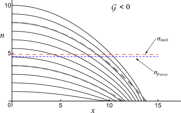
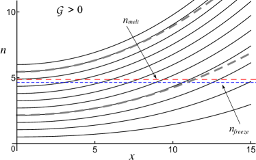
Fig.  1: Typical form of the density profile $n(x;n_{0})$ (solid lines) of “soft spheres” for “attractive” (${\mathcal{G}}<0$, left panel) or “repulsive” (${\mathcal{G}}>0$, right panel) Marangoni flow. The horizontal lines correspond to the values $n_{\mathrm{freeze}}$ and $n_{\mathrm{melt}}$, at which the phase transitions occur. The dashed lines show, for each of the cases ${\mathcal{G}}\gtrless 0$, two examples of the parabolic approximation given by Eqn (16).

The stationary state of the monolayer ($\partial\varrho/\partial t=0$) is given by the condition

$${\bf v}=0\qquad\Rightarrow\qquad-\Gamma\nabla\mu+{\bf u}=0.$$ (4)

Since ${\bf u}$ is given by Eqn (2c), this is an integrodifferential equation for the stationary profile $\varrho({\bf r})$. However, the mathematical analogy with gravity, expressed by Eqn (3), allows one to reduce Eqn (4) to a partial differential equation for the profile: taking the divergence of Eqn (4) renders

$$-\Gamma\nabla^{2}\mu(\varrho)+{\mathcal{G}}\varrho=0.$$ (5)

This equation must be complemented by the appropriate boundary conditions. The form of the Marangoni flow (2c) assumes that the fluid occupies an unbounded domain, i.e., we assume implicitly that there is no relevant influence by the distant boundary conditions and look, therefore, for radially symmetric solutions expressing spatial isotropy. In experiments, for instance, one can think of a monolayer confined laterally by a distant circular hard wall. Alternatively, one can also consider a circular optical trap or a coarse circular sieve that confines the particles only without disrupting appreciably the ambient flow or the sources of the Marangoni flow (distribution of chemicals or temperature gradients). It is thus still meaningful to study solutions to Eqn (5) for a monolayer of a finite spatial extent, say $r<{\cal L}$, while using the expression (2c) for flow in an unbounded region.

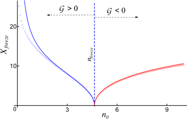
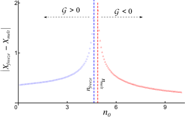
Fig.  2: (Left) The value of the radial distance $X_{\mathrm{freeze}}$ from the center at which the freezing transition in “soft spheres” occurs for each profile (labelled by the value $n_{0}$ of the central density). The solid line is the approximation given by Eqn (17). (Right) Plot of the width $|X_{\mathrm{freeze}}-X_{\mathrm{melt}}|$ of the region where the hexatic phase occurs. In both plots, the branch with $n_{0}>n_{\mathrm{freeze}}$ corresponds to the case of “attractive” Marangoni flow; the other branch is associated to the “repulsive” case.

Irrespective of the exact form of these distant boundary conditions, we look for radially symmetric solutions, for which Eqn (5) takes the form

$$\left(\frac{d^{2}}{dr^{2}}+\frac{1}{r}\frac{d}{dr}\right)\mu(\varrho(r))=\frac{{\mathcal{G}}}{\Gamma}\varrho(r).$$ (6)

We look for solutions that are regular (continuous and differentiable); this imposes additional boundary conditions at the origin of the coordinate system, namely,

$$\varrho(r=0)=\varrho_{0}\;\mathrm{finite},\qquad\frac{d\varrho}{dr}(r=0)=0.$$ (7)

Let $T$ denote the temperature ($k$ will be Boltzmann’s constant) and $\varrho_{c}$ denote a characteristic density of the phases described by the chemical potential $\mu$. We introduce the dimensionless magnitude

$${g}:=\frac{{\mathcal{G}}}{\Gamma kT},$$ (8)

which pertains only to the hydrodynamical effects, and the length scale

$$\ell:=\frac{1}{\sqrt{|{g}|\varrho_{c}}},$$ (9)

which represents the characteristic mean interparticle separation $1/\sqrt{\varrho_{c}}$ rescaled by the hydrodynamic factor (8). With the definitions

$$x:=\frac{r}{\ell},\qquad n:=\frac{\varrho}{\varrho_{c}},\qquad\hat{\mu}(n):=\frac{\mu(\varrho)}{kT},$$ (10)

of dimensionless variables, we arrive finally at an initial value problem for an ordinary differential equation:

$$\left(\frac{d^{2}}{dx^{2}}+\frac{1}{x}\frac{d}{dx}\right)\hat{\mu}(n(x))=\operatorname{sign}{({\mathcal{G}})}n(x),$$ (11a)

$$n(x=0)=n_{0}\;\mathrm{finite},\qquad\frac{dn}{dx}(x=0)=0.$$ (11b)

This determines the density profile $n(x;n_{0})$, which is actually identified uniquely by the value $n_{0}$ of the central density. From this profile, the total amount of particles contained within a disk of a given radius ${\cal L}$ is calculated as

$$M({\cal L}):=2\pi\int_{0}^{\cal L}dr\;r\varrho(r)=\frac{2\pi}{|{g}|}N(X),$$ (12a)

where

$$N(X;n_{0}):=\int_{0}^{X}dx\;x\,n(x;n_{0}),\qquad X:=\frac{\cal L}{\ell}.$$ (12b)

The Marangoni flow, which has the radial direction ${\bf e}_{r}$, can then be computed by a straightforward application of Gauss theorem to Eqn (3),

$${\bf u}({\bf r})=\frac{{\mathcal{G}}M(r)}{2\pi r}{\bf e}_{r}.$$ (13)

When this expression is combined with the stationarity condition (4) and the definition (12a), one gets

$$N(X;n_{0})=\operatorname{sign}{({\mathcal{G}})}X\;\frac{d\hat{\mu}(n(X;n_{0}))}{dn}\;\frac{dn(X;n_{0})}{dX}.$$ (14)

This expression provides a relationship between the three parameters $n_{0}$, $N$ and $X$ (that is, $\varrho_{0}$, $M$, and ${\cal L}$ in physical variables). Therefore, concerning an experimental realization, any stationary state can be characterized by the measurement either of the central density $\varrho_{0}$ or of the total number of particles $M$ within a finite circular region of radius ${\cal L}$. Alternatively, when preparing the system in the laboratory, one can fix the amount $M$ of particles in a region defined by its size ${\cal L}$ (which may be significantly easier to control than the value of $\varrho_{0}$). This flexibility in choosing the variables is particularly important for connecting the theoretical analysis with the experimentally accessible quantities since, from the point of view of numerical analysis, the solution $n(x;n_{0})$ of equations (11) is most conveniently parametrized by the value $n_{0}$ of the density at the center of the domain.

3 Results and discussion

We are now in a position to apply the generic framework developed above to specific cases that are experimentally relevant. Since the Marangoni flow can be formally analogous to Newtonian gravity, the stationary profiles that solve Eqn (5) would be the equivalent of a material cluster in equilibrium under its own gravity. The thermodynamic properties of the monolayer enter via the chemical potential $\hat{\mu}(n)$. If this includes the existence of different equilibrium phases, one can then easily envision the emergence of a radially stratified structure, much like in the postulated interior of condensed astrophysical objects (planets and stars).

We therefore will consider the solution to equations (11) for different choices of the chemical potential. We shall focus on two extreme cases that intend to describe experimentally relevant systems. In one extreme, there is the case of “soft spheres”, in which particles experience a mutual long–ranged repulsive interaction. In the opposite extreme there is the limit of hard spheres, for which the repulsion is very short–ranged.

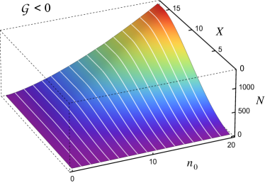
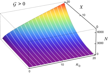
Fig.  3: The function $N(X;n_{0})$, i.e., the total amount of “soft spheres” inside a circular region of given radius, for “attractive” (${\mathcal{G}}<0$, left panel) or “repulsive” (${\mathcal{G}}>0$, right panel) Marangoni flow. Each white line corresponds to a curve $N(X)$ for a given constant value of $n_{0}$.

3.1 Soft spheres

As a first case study, we model the colloidal particles as “soft–spheres”, a term that characterizes particles that interact with each other by means of a repulsive power–law potential. More precisely, we consider a pair potential of the form

$$V_{\mathrm{dip}}(r)=\frac{B}{r^{3}}=kT\left(\frac{\zeta}{r}\right)^{3},$$ (15)

where the constant $B$ — or equivalently, the parameter $\zeta=(B/kT)^{1/3}$ (Bjerrum length) — characterizes the strength of the interaction. This potential can model the dipolar repulsion due to the induced moments in paramagnetic particles immersed in an external magnetic field ⁴⁵. It can also describe the asymptotic repulsion between electrically charged particles when one of the fluids is a dielectric ^{56, 57, 58, 59, 60, 61}, or between polarized particles in an external electric field ⁴⁷. The evaluation of the partition function leads straightforwardly to the simple scaling form $\mu(\varrho,T)=kT\hat{\mu}(\varrho\zeta^{2})$ of the chemical potential; this provides the function $\hat{\mu}(n)$ in Eqn (10) with the natural choice $\varrho_{c}:=\zeta^{-2}$ as characteristic density (see Appendix A). This scaling form implies that the phase diagram is particularly simple because it does not depend on two independent control parameters (density and temperature). Instead, the only relevant parameter is the combination given by the rescaled density $n=\varrho\zeta^{2}$.

Particles interacting with Eqn (15) are known to exhibit a discontinuous liquid–solid phase transition in 3D ⁶². In 2D, however, it was predicted (the Kosterlitz–Thouless–Halperin–Nelson–Young theory ^{63, 64, 65}) that a hexatic phase exists, so that freezing occurs continuously in the variable $n$ in two stages, first a liquid–hexatic, and then a hexatic–solid transition. This scenario has been confirmed recently in experiments involving monolayers of paramagnetic particles ⁴⁵ and monolayers of electrically charged particles ⁴⁶. The range of existence of the hexatic phase is very narrow: according to the experimental values quoted by ref. ⁴⁵, the liquid–hexatic transition (“liquid freezes”) occurs at $n_{\mathrm{freeze}}\approx 4.65$, while the hexatic–solid transition (“solid melts”) takes place at $n_{\mathrm{melt}}\approx 4.87$ (the corresponding values quoted in ref. ⁴⁶ are somewhat larger; this may be due to uncertainties in the determination of the value of $\zeta$ in Eqn (15)).

The density profile $n(x;n_{0})$ is obtained by solving equations (11) numerically with the fit to the chemical potential $\hat{\mu}(n)$ given by Eqn (29). Fig. 1 shows a representative set of profiles. For not too small values of the central density $n_{0}$, we find that, in the region of nonvanishing densities, the profile is very well approximated by its parabolic approximation about the center:

$$n(x;n_{0})\approx n_{0}\left[1+\operatorname{sign}{({\mathcal{G}})}\left(\frac{x}{\lambda}\right)^{2}\right],\qquad\lambda(n_{0}):=2\sqrt{\frac{d\hat{\mu}}{dn}(n_{0})}.$$ (16)

(The coefficient $\lambda$ is straightforwardly obtained by looking for a solution to the differential equation (11a) in the form of a Taylor expansion.) When ${\mathcal{G}}<0$ (“attractive” Marangoni flow), the density increases towards the center of the distribution (as for an astrophysical object under its own gravity). One thus expects to observe different local structures, corresponding to the phase associated with the local value of $n$, in an “onion-like” assembly. So, there would be crystalline order near the center, surrounded by a disordered isotropic fluid; and between both phases, there should appear a hexatic shell exhibiting orientational, but not positional, order. The trend is reversed when ${\mathcal{G}}>0$ (“repulsive” Marangoni flow).

Another interesting feature is that in the “atractive” case the system is “self–confined” in the following sense. Since the density decays steadily to zero, the farther the external walls are located, the smaller (vanishing) is the confining pressure exerted by them. This is a direct consequence of the long–ranged nature of the Marangoni flow given by Eqn (2c): in the language of Statistical Mechanics, this (“gravitational”) force is nonintegrable and, provided the system is large enough, dominates over the short–ranged dipolar repulsion given by Eqn (15). In the opposite case of “repulsive” Marangoni, it is obvious that the walls are required to confine the system against the Marangoni and dipolar repulsions: this explains the formation of a fluid (low density) central region in the profiles shown in Fig. 1 and a crystalline (high density) structure at the outer border.

In Fig. 2 we show the radial distance $X_{\mathrm{freeze}}(n_{0})$ from the center at which the freezing transition is expected to occur as a function of the central density $n_{0}$, i.e., the solution of $n(X_{\mathrm{freeze}};n_{0})=n_{\mathrm{freeze}}$. The prediction given by the approximated profile (16), namely

$$X_{\mathrm{freeze}}(n_{0})\approx\lambda(n_{0})\left|\frac{n_{0}}{n_{\mathrm{freeze}}}-1\right|^{1/2},$$ (17)

provides an excellent fit for any central density $n_{0}>2$, and captures the divergence as $n_{0}\to 0$. Similarly, one defines the radial distance $X_{\mathrm{melt}}(n_{0})$ at which the melting transition occurs. Also shown in Fig. 2 is the width $|X_{\mathrm{freeze}}-X_{\mathrm{melt}}|$ of the shell where the hexatic phase would be observed.

Starting from the profiles $n(x;n_{0})$ parametrized by the value of $n_{0}$, one can compute the function $N(X;n_{0})$ given by Eqn (12b). Figure 3 shows this function for different values of $n_{0}$. In the range of parameters explored, the curves do not cross and seem to cover the whole $(X,N)$ plane. This means that the preparation of a system with given $N$ and $X$ determines $n_{0}$ uniquely, and that all the combinations of the parameters $N$ and $X$ lead to a solution of equations (11), i.e., to a stationary state. This is not a trivial statement: for instance, it is long known in the astrophysical community that a self–gravitating ideal gas (the so-called “isothermal sphere” configuration) can lack stationary states, depending on the values of the parameters (see, e.g., the review work ⁶⁶). However, this behavior is usually seen as a limitation of the ideal gas approximation. Our numerical results for particles with the interaction potential (15) confirm this expectation.

Fig.  4: Typical density profiles $n(x;n_{0})$ of hard spheres for “attractive” (left) or “repulsive” (right) Marangoni flow.

3.2 Hard spheres

We now consider the case that the colloidal particles are approximated as “hard–spheres”, i.e., their only interaction is hard–core exclusion. The chemical potential for this system also exhibits a simple scaling (see Appendix B), $\mu(\varrho,T)=kT\hat{\mu}(\varrho/\varrho_{c})$, with the close–packing number density $\varrho_{c}=1/(2\sqrt{3}R^{2})$ of disks of radius $R$. This system does not exhibit any phase transition, staying in a fluid phase for any density $n=\varrho/\varrho_{c}<1$. The limiting value $n=1$ can only be reached under infinite pressure and corresponds to the formation of a crystal of hard disks in contact.

The density profiles $n(x;n_{0})$, shown in Fig. 4, are obtained by solving equations (11) numerically with the fit to the chemical potential $\hat{\mu}(n)$ given by Eqn (31). The profiles for which $n(x;n_{0})$ is never close to one describe a smoothly varying distribution. However, for those which come close to $n=1$ (either at the center for “attractive” Marangoni flow or far from it for “repulsive” Marangoni flow), the most salient feature is an apparent phase segregation: a closely–packed crystalline structure emerges in coexistence with a dilute “gas phase”. (The exactly close packed structure with $n=1$ is never reached, but the difference would be visually unnoticeable in an experimental realization.) The transition region between both phases has a nonvanishing width (as remarked, the hard–disk system does not have a true phase transition in the thermodynamic sense), but the width can be substantially smaller than the extension of the “crystal” and the “gas”. This would give the impression of a pseudotransition between two phases. For this kind of configurations, we have found that the radial position $X_{\mathrm{trans}}$ of this pseudotransition can be defined conventionally by the location of the inflection point of the density profile, i.e., $n^{\prime\prime}(X_{\mathrm{trans}};n_{0})=0$. In Fig. 5 we show this position as a function of the central density. We remark on passing that these profiles would correspond to the core–halo structures reported in the study of the equilibrium configurations of a self–gravitating 3D gas of hard spheres ^{66, 67, 68}.

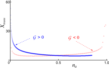
Fig.  5: The position of the pseudotransition in the case of hard spheres as a function of the central density.

The function $N(X;n_{0})$ given by Eqn (12b) has been evaluated for each density profile, identified by the central density $n_{0}$. The results are shown in Fig. 6. The line $N(X;1)=X^{2}/2$ (best visible in the case of ${\mathcal{G}}<0$ as the border of the white region in the back vertical plane) represents the border of the physically accessible region, i.e., beyond which the total packing fraction is higher than close packing (one cannot pour in more hard particles than actually fit in the region). The curves $N(X;n_{0})$ seem to cover completely the interior of the physically accessible region without mutual crossing. Thus, the relationship between the central density $n_{0}$ and the pair $(X,N)$ is one-to-one in the explored range of values.

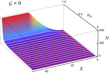
Fig.  6: The function $N(X;n_{0})$, i.e., the total amount of “hard–core spheres” inside a circular region of given radius, for “attractive” (${\mathcal{G}}<0$, left panel) or “repulsive” (${\mathcal{G}}>0$, right panel) Marangoni flow. Each white line corresponds to a curve $N(X;n_{0})$ for constant $n_{0}$.

3.3 Experimental relevance

We now consider the theoretical predictions derived in the previous Sections from the perspective of potential experimental validation. For that purpose, we focus on the more interesting case of the soft repulsive interaction and provide numerical estimates for the various parameters appearing in the theoretical model. Additionally, this provides the means to critically assess the validity of the assumptions involved in the model.

In order to translate the results derived in the previous Sections into physical units, we have to compute the characteristic density scale $\varrho_{c}=\zeta^{-2}$ and the characteristic length scale $\ell=1/\sqrt{|g|\varrho_{c}}=\zeta/\sqrt{|g|}$, see Eqn (9). More precisely, since equations (2) provide a coarse–grained description, one would ideally require that the characteristic length $\ell$ is much larger than the mean interparticle separation, i.e.,

$$\ell\sqrt{\varrho}=\frac{\ell\sqrt{n}}{\zeta}=\sqrt{\frac{n}{|g|}}\gg 1.$$ (18)

Additionally, the model equations have been obtained in the dilute approximation; this requires that the mean interparticle separation is much larger than the radius $R$ of the particles, i.e.,

$$\frac{1}{R\sqrt{\varrho}}=\frac{\zeta}{R\sqrt{n}}\gg 1.$$ (19)

These two constraints set the limits of applicability of the theoretical predictions. Although they depend locally on the value of the density $n$, they do so weakly; thus, for the purpose of getting order-of-magnitude estimates, one can simply set $n=1$ in equations (18) and (19). Therefore, Eqn (18) states that the activity cannot be too large, while Eqn (19) states that the repulsion between the soft spheres cannot be too weak.

The value of the parameter $\zeta$, which sets the mean interparticle separation, depends on the specific physical origin of the repulsion given by Eqn (15). We consider here its value in some representative physical systems that have been previously studied:

1. In the experimental setup with paramagnetic particles reported in ref. ⁴⁵, it is (see ref. ⁶⁹)

   $$\frac{\zeta}{R}\approx 2.30\left(\frac{H}{\mathrm{hA/m}}\right)^{2/3}\frac{R}{\mathrm{\mu m}},$$ (20)

   with an applied magnetic field in the range $H\approx 1$–$10\;\mathrm{hA/m}$ ($\mathrm{hA}=10^{2}\;\mathrm{A}$ is hecto-ampere; the lowest bound is set by Earth’s magnetic field of strength $\approx 0.4\;\mathrm{hA/m}$).

2. For the case of particles polarized by an external electric field $E$, one has (see ref. ⁶⁹)

   $$\frac{\zeta}{R}\approx 3.74\left(\frac{E}{\mathrm{MV/m}}\right)^{2/3}\frac{R}{\mathrm{\mu m}},$$ (21)

   when the parameter values of the experiment reported in ref. ⁴⁷ are used (here $\mathrm{MV}=10^{6}\;\mathrm{V}$ is mega-volt).

3. Polymeric or dielectric oxide (e.g., silica, titania, alumina) colloidal particles immersed in water generically become ionized. When, additionally, they are trapped at the interface between water and a dielectric fluid (e.g., air or oil), their mutual interaction takes the form of Eqn (15). For polystyrene particles at a water–oil interface, as in the experimental configuration employed in ref. ⁶¹, and assuming weakly charged colloids, we derive the estimate (see Appendix C)

   $$\frac{\zeta}{R}\approx 0.59\left(\frac{\mathrm{M}}{c}\,\frac{R}{\mathrm{\mu m}}\right)^{1/3},$$ (22)

   where $c$ is the molar (M) concentration of the monovalent ions in water. If the charge of the particles is very large, nonlinear screening effects dominate and the estimate (22) is invalid because the Bjerrum length becomes almost independent of the ionic concentration of the solution ⁵⁹.

The parameter ${g}$ gives the magnitude of the Marangoni flow, Eqs. (2c) and (8). Its sign will depend on how the surface tension of the interface is influenced by the chemical or thermal activity of the particles and on whether the particles are sources or sinks of that tensioactive component. Thus, one gets an “attractive” Marangoni flow (${g}<0$) for chemically active particles either (i) if the surface tension decreases with increasing concentration of the chemicals and the latter are released by the particles or (ii) if the surface tension increases and the chemicals are adsorbed by the particles ^{51, 42}. For thermally active particles, this “attractive” effect is achieved when either (i) the particles are sources of heat and the surface tension is reduced with increasing temperature, or (ii) the particles absorb heat and the surface tension grows with temperature ^{38, 52}. The trends must be reversed in order to achieve a “repulsive” Marangoni flow (${g}>0$).

In order to be definite, one can estimate $g$ for the cases of activity that have been discussed in experimental reports. Thus, for platinum–covered active particles catalysing the decomposition of water peroxide we get (see App. D)

$$|{g}|\approx 0.075\left(\frac{R}{\mathrm{\mu m}}\right)^{3},$$ (23)

when an air–water interface is considered. For an interface between two dense fluids (like water and oil, as in the experiments reported in ref. ³⁶), this value is expected to be enhanced by up to four orders of magnitude due to the reduced diffusivity of molecular oxygen in the liquid phases compared to the one in a gas phase ⁴². For particles that become thermally active due to heating by a laser, the value of $g$ for micron–sized particles is larger by over six orders of magnitude (see App. D).

By combining this estimate of ${g}$ with any of the previous estimates of the Bjerrum length $\zeta$, one can check the fulfillment of the constraints (18) and (19). This is illustrated in Fig. 7, which shows the region in parameter space where the constraints are expected to hold. The left plot corresponds to ionizable particles, with $\zeta$ given by Eqn (22); the right plot to paramagnetic particles with $\zeta$ given by Eqn (20). (The plot obtained with the estimate (21) for electrically polarized particles is essentially indistinguishable from the right plot when the vertical axis is reinterpreted as electric field measured in $\mathrm{MV/m}$.)

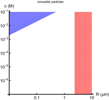
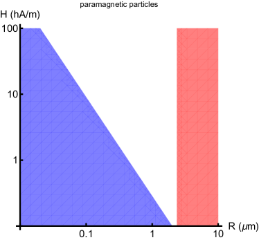
Fig.  7: The parameter space for different experimental realizations. The unshadowed area is the parameter region where the constraints given by Eqs. (18) and (19) (with $n=1$) are expected to hold. The red area represents the region where $\ell/\zeta<1$, the activity $g$ being estimated with Eqn (23). In the blue area it is $\zeta/R<1$, with $\zeta$ estimated from Eqn (22) for the left plot, and from Eqn (20) for the right one.

We remark here that we are not in a position to tackle the specific details of an actual experimental realization, for instance, how a platinum–covered active particle can be fabricated that is paramagnetic or remains ionizable. Thus, the results shown in Fig. 7 have to be understood as a rough guide for the search of an optimal experimental configuration. In this regard, the plots suggest that there are experimentally accessible ranges of parameter values where the model is valid and the theoretical predictions can be tested. Consider, for instance, a collection of ionizable particles of radius $R=0.5\;\mathrm{\mu m}$ at a water–oil interface with $c=10^{-6}\;\mathrm{M}$ (for pure water). In this case, $\zeta\approx 46R$, and thus the dilute approximation is well grounded. The corresponding characteristic length $\ell$ is also large, i.e., $\ell\approx 10\zeta$, and thus the full “onion-like” structure of crystalline core, fluid phase, and hexatic transition region, see Figs. 1 and 2, should be experimentally accessible. Similarly, paramagnetic particles of the same radius at a water–air interface in a large magnetic field $H=10^{2}\;\mathrm{hA/m}$ would give the values $\zeta\approx 25R$ and $\ell\approx 10\zeta$; such system thus provides another potential candidate for an experimental validation of the theoretical predictions.

We finally notice that the flow given by Eqn (13) would likely be not directly observable. The characteristic velocity scale is $\Gamma kT/\ell$, as derived from equations (12). For the examples considered above, this scale lies in the range of nanometers per second. Therefore, the effect of the activity of the particles would not be so much apparent in the induced Marangoni flow as in the “onion-like” structure of phase coexistences.

4 Conclusions

We have studied a mean–field model for the phase coexistence in a monolayer of colloidal particles with repulsive interactions, located at a fluid interface, and experiencing Marangoni flow induced by the activity of the particles. We have analyzed in detail the case of “soft” (decaying as $r^{-3}$) and hard–core repulsive interactions. We have found stationary states with an “onion-like” structure in the particle distribution within the monolayer. For the most relevant case of soft repulsion, the density reaches the values corresponding to the liquid to hexatic (freezing) and solid to hexatic (melting) transitions in two dimensions, respectively. Furthermore, we have thoroughly and critically discussed the relevance of these results for potential experimental realizations and concluded that experimental validation of the theoretical predictions seems feasible.

A further interesting consequence of the constraints expressed by Eqs. (18) and (19) is that they lead to opposing restrictions on the size of the colloidal particles, with the radius $R$ being typically bracketed between a maximum and a minimum value (see Fig. 7). A weak Marangoni flow expands the range of values of $R$ for validity of the theoretical results. It was noticed in ref. ⁴² that the small value $g\sim 0.01$–$0.1$ in usual configurations could explain the lack of experimental observations of the activity–induced Marangoni flow. However, the Marangoni flow has a long–ranged component formally analogous to gravity. As a consequence, these lead to the interesting aspect that, although the drag velocity by the Marangoni flow may be unobservably small, the added-up effect of many particles yields noticeable collective effects (see, e.g., the qualitative discussion on this issue in ref. ⁶⁹). Therefore, the most relevant conclusion of this work is that the spatially structured phase coexistence is the observationally accessible signature of the activity–induced Marangoni flow.

When this flow is too strong, the constraint in Eqn (18) is not satisfied, which usually hints that the mean–field expression (2c) is a poor approximation and that interparticle correlations have to be accounted for in the computation of the Marangoni flow. Likewise, violation of the constraint in Eqn (19) indicates that hydrodynamical interactions other than the Marangoni flow, here including short–ranged corrections, have to be considered. Both scenarios call for a cautionary use of the notion of “phase coexistence”, since a phase is a well–defined concept in equilibrium thermodynamics only. Its use in the context of the addressed problem is meaningful thanks to the wide separation of length scales expressed by Eqs. (18) and (19): in such case, one can apply the hypothesis of local equilibrium in order to comprise the relevant contribution by the interparticle direct forces into the equilibrium chemical potential $\mu(\varrho)$. This latter function then provides the ground for the notion of a local “thermodynamic phase”.

When the length scales are not well separated, it may not be appropriate to interpret the features of a stationary density profile in terms of thermodynamic phases. This, however, opens up the possibility of an exciting new scenario, namely that those features actually represent the nonequilibrium counterpart of “phases” which are induced by the hydrodynamic interactions. For instance, the crystal–gas profiles derived for hard–spheres (see Fig. 4) clearly violate the dilute–limit approximation and the theoretical model must be modified in order to provide reliable predictions. Thus, the analysis presented in Sec. 3.2 should be viewed as a first step towards a more realistic model that accounts for the changes in the “crystal–gas–coexistence” interpretation which would be induced by the short–ranged hydrodynamic interactions.

Appendix A Appendix: equation of state for soft spheres

Under isothermal conditions, the chemical potential of the particles in the monolayer, $\mu(\varrho,T)$, can be related to the equation of state $p(\varrho,T)$ for the pressure by means of the thermodynamic identity

$$\left(\frac{\partial\mu}{\partial\varrho}\right)_{T}=\frac{1}{\varrho}\left(\frac{\partial p}{\partial\varrho}\right)_{T}.$$ (24)

The evaluation of the partition function for a collection a particles interacting with the potential given by Eqn (15) straightforwardly leads to the scaling relationship $p(\varrho,T)=kT\zeta^{-2}\hat{p}(n)$ with $n=\varrho\zeta^{2}$. Then, the expression (24) renders $\mu(\varrho,T)=kT\hat{\mu}(n)$. This scaling (which is shared with the hard spheres case) shows that the collection of soft spheres is an athermal system, i.e., its phase diagram depends only on density, not on temperature.

The equation of state $\hat{p}(n)$ can be determined by a combination of numerical results and theoretical estimates. Thus, Monte Carlo simulations ⁶⁹ show that the following fit holds to a good approximation in the high density range of the fluid phase:

$$\hat{p}_{\mathrm{fluid}}(n)=n(3+6.6n^{3/2}),\qquad 2\lesssim n<n_{\mathrm{freeze}},$$ (25)

where $n_{\mathrm{freeze}}\approx 4.65$ is the density at the freezing transition. In the solid phase, theoretical arguments confirmed by comparison with numerical results ⁷⁰ suggest a fitting of the form

$$\hat{p}_{\mathrm{solid}}(n,T)=n\left(\frac{5}{2}+Kn^{3/2}\right),\qquad n_{\mathrm{freeze}}<n.$$ (26)

with a certain constant $K$. This analysis neglects the existence of a hexatic phase between the liquid and the solid ones, given that the range of existence is very narrow ($n_{\mathrm{melt}}-n_{\mathrm{freeze}}\approx 0.22$). One can provide an estimate of the value of $K$ by imposing ad hoc the condition that the fluid and solid phases coexist at the freezing density:

$$\hat{p}_{\mathrm{fluid}}(n_{\mathrm{freeze}})=\hat{p}_{\mathrm{solid}}(n_{\mathrm{freeze}})\qquad\Rightarrow\qquad K\approx 6.65.$$ (27)

Since $\hat{p}_{\mathrm{solid}}>442$, the relative error committed in estimating the pressure $\hat{p}_{\mathrm{solid}}$ of the solid phase with the fitting formula $\hat{p}_{\mathrm{fluid}}$ for the high–density fluid is less than $1\%$. Therefore, it can be assumed

$$\hat{p}(n)=n(3+6.6n^{3/2}),\qquad 2\lesssim n,$$ (28)

in the whole range of high densities, regardless of the phase being considered. For low densities, $n<2$, this fit departs from the values derived from simulations. However, the deviations are not very large (e.g., less than $25\%$ if $n>0.5$) and, indeed, we have checked that the profiles shown in Fig. 1 are practically indistinguishable when either the simulation data or the extrapolation of Eqn (28) down to $n\to 0$ are used to compute them. Therefore, for our purposes one can use the chemical potential obtained by integrating Eqn (24) with Eqn (28) for the whole range of densities considered in this work:

$$\hat{\mu}(n)=3\ln n+11n^{3/2}+\mu_{0},$$ (29)

with an irrelevant integration constant $\mu_{0}$.

Appendix B Appendix: equation of state for hard spheres

The equation of state of hard spheres exhibits the simple scaling $p(\varrho,T)=kT\varrho_{c}\hat{p}(n)$, with $n=\varrho/\varrho_{c}$ in terms of the close packing density $\varrho_{c}$. This carries over to a scaling $\mu(\varrho,T)=kT\hat{\mu}(n)$ for the chemical potential via Eqn (24). Thus, the monolayer of hard spheres is an athermal system and its phase behavior depends only on density. For our purposes, it is sufficient to use the approximate equation of state of a two–dimensional fluid of hard spheres (i.e., hard disks) provided by ref. ⁷¹:

$$\hat{p}(n)=n\frac{1+n}{1-n},$$ (30)

with $\varrho_{c}=1/(2\sqrt{3}R^{2})$ denoting the close packing density for disks of radius $R$. This leads to the chemical potential

$$\hat{\mu}(n)=\ln\frac{n}{(1-n)^{2}}+\frac{2}{1-n}+\mu_{0},$$ (31)

with an irrelevant integration constant $\mu_{0}$.

Appendix C Appendix: Bjerrum length for ionizable particles

When ionizable particles are trapped at the interface between water and a dielectric fluid, they experience a mutual long–ranged repulsion because, unlike in bulk water, the electric field is not completely screened. This repulsion follows Eqn (15) because each particle can be modelled as an electric dipole perpendicular to the interface ^{56, 57, 60}. Although this expression is justified in principle only as an asymptotic approximation between sufficiently distant pairs, its validity has been confirmed experimentally ^{58, 61}. Of particular interest for our purposes is that the interaction can be actually described well with Eqn (15) for a wide range of monolayer densities that includes the ones of the transitions involving the hexatic phase ^{61, 46}.

If the total charge $q$ of the particle is sufficiently small, linear screening holds and the strength of the dipole is proportional to the product of the charge $q$ with the Debye length $\kappa^{-1}$ in water ^{56, 57}. As a consequence, the proportionality constant $B$ in Eqn (15) satisfies the scaling $B\propto(q/\kappa)^{2}$. For a symmetric electrolyte, the Debye length depends on the concentration $c$ of monovalent ions as $\kappa\propto\sqrt{c}$. Assuming that the charged acquire by the particle is proportional to its surface, one arrives at the relation

$$B=\hat{B}\frac{R^{4}}{c}.$$ (32)

The constant $\hat{B}$ can be estimated, for instance, from the experimental study described in ref. ⁶¹: the value $B/kT\approx 2\times 10^{5}\,\mathrm{\mu m}^{3}$ is measured, which is of the same order of magnitude as previously reported values, when using polystyrene particles of radius $R=1\;\mathrm{\mu m}$ trapped at an interface between oil and very pure water, for which we take the conservative estimate $c=10^{-6}\;\mathrm{M}$. The expression in Eqn (32) then leads to the estimate, Eqn (22), for the Bjerrum length.

Appendix D Appendix: strength of the Marangoni flow

In order to get a quantitative estimate of the strength $g$ of the Marangoni flow, we start from the detailed calculation in the point–particle (monopolar) approximation. For a chemically active particle, the computation shows that the magnitude of the Marangoni flow, as appears in Eqn (2c), is ⁴²

$${\mathcal{G}}=\frac{Qb_{0}}{8D_{+}\eta_{+}}.$$ (33)

Here, $Q$ denotes the source/sink (monopole) strength of the active particle, i.e., the amount of chemical released/absorbed by an active a particle per unit time. $b_{0}$ denotes the coefficient of the linear response of the surface tension to changes in the concentration of chemical species or in temperature at the interface, while $\eta_{+}$ and $D_{+}$ are average values of the viscosity and of the diffusion constant of chemicals in the two fluids, respectively. The expression for the case of a thermally active particle is exactly the same ^{38, 52} with the reinterpretation of $Q$ as the heat exchanged per unit time between the particle and the fluids, of $b_{0}$ as the surface tension response to temperature changes, and of $D_{+}$ in terms of the heat conductivities of the fluids.

In the dilute limit, which is implicit in our model, the mobility $\Gamma$ can be approximated by the Stokes formula for a sphere of radius $R$ in a fluid of viscosity $\eta_{+}$. Then, from Eqs. (8) and (33 one arrives at

$${g}=\frac{3\pi Qb_{0}R}{4D_{+}kT}.$$ (34)

The dependences on the details of the activity and on the effect of the active component on the surface tension makes difficult to estimate the value of ${g}$. We have thus considered for definiteness two specific configurations, for chemically or thermally active particles, respectively:

1. For chemically active particles, we note that ${g}$ in Eqn (34) is a factor of 25 larger than the similar quantity $q$ estimated in ref. ⁴², so that one can straightforwardly adapt the available estimates for $q$ to the problem of interest here. Thus, for an active particle made of platinum and decomposing hydrogen peroxide dissolved in the fluids, for which $Q/(4\pi R^{2})\approx 10^{-3}\;\mathrm{mol/(s\times m^{2})}$ in the experiment described in ref. ⁵, one obtains the estimate quoted in Eqn (23) for an air–water interface, corresponding to the values $D_{+}\sim 10^{-4}\;\mathrm{m^{2}/s}$, $\eta_{+}\sim 10^{-3}\;\mathrm{Pa\times s}$, $b_{0}\sim 10^{-3}\;\mathrm{N/(m\times M)}$.

2. For thermally active particles, we refer to the simulations reported in ref. ⁷² of a self–propelled particle due to it being heated by a laser. For micron–sized particles, this provides a temperature gradient of the order of $1\;\mathrm{K/\mu m}$ in the fluid close to the particle. Since the temperature contrast $\Delta T(r)$ at a distance $r$ from the particle is given as $\Delta T=Q/(4\pi D_{+}r)$ in the monopolar approximation ^{52, 42}, we estimate $Q/(4\pi D_{+})\approx 1\;\mathrm{K\times\mu m}$. Therefore, for $R=1\;\mathrm{\mu m}$ and $b_{0}\approx-2\times 10^{-4}\;\mathrm{N/(m\times K)}$ for an air–water interface, Eqn (34) gives a value of $g$ which is $10^{6}$ times larger than the case of the chemically active particle.

Appendix E Acknowledgements

A.D. acknowledges support by the Ministerio de Economía y Competitividad del Gobierno de España through Grant FIS2017-87117-P (partially financed by the European Regional Development Fund). This article is based upon work from COST Action MP1305 “Flowing Matter”, supported by COST (European Cooperation in Science and Technology). The authors thank Martin Oettel for providing the MC simulations data.

References

- Lauga and Powers 2009 E. Lauga and T. Powers, Rep. Prog. Phys., 2009, 72, 096601.
- Ebbens and Howse 2010 S. Ebbens and J. Howse, Soft Matter, 2010, 6, 726–738.
- Elgeti et al. 2015 J. Elgeti, R. Winkler and G. Gompper, Rep. Prog. Phys., 2015, 78, 056601.
- Bechinger et al. 2016 C. Bechinger, R. Di Leonardo, H. Löwen, C. Reichhardt, G. Volpe and G. Volpe, Rev. Mod. Phys., 2016, 88, 045006.
- Paxton et al. 2004 W. Paxton, K. Kistler, C. Olmeda, A. Sen, S. Angelo, Y. Cao, T. Mallouk, P. Lammert and V. Crespi, J. Am. Chem. Soc., 2004, 126, 13424.
- Golestanian et al. 2005 R. Golestanian, T. Liverpool and A. Ajdari, Phys. Rev. Lett., 2005, 94, 220801.
- Howse et al. 2007 J. Howse, R. Jones, A. Ryan, T. Gough, R. Vafabakhsh and R. Golestanian, Phys. Rev. Lett., 2007, 99, 048102.
- Rückner and Kapral 2007 G. Rückner and R. Kapral, Phys. Rev. Lett., 2007, 98, 150603.
- Jülicher and Prost 2009 F. Jülicher and J. Prost, Eur. Phys. J. E, 2009, 29, 27.
- Popescu et al. 2009 M. N. Popescu, S. Dietrich and G. Oshanin, J. Chem. Phys., 2009, 130, 194702.
- Popescu et al. 2010 M. N. Popescu, S. Dietrich, M. Tasinkevych and J. Ralston, Eur. Phys. J. E, 2010, 31, 351.
- ten Hagen et al. 2011 B. ten Hagen, S. van Teeffelen and H. Löwen, J. Phys.: Condens. Matter, 2011, 23, 194119.
- Sabass and Seifert 2012 B. Sabass and U. Seifert, J. Chem. Phys., 2012, 136, 064508.
- Sharifi-Mood et al. 2013 N. Sharifi-Mood, J. Koplik and C. Maldarelli, Phys. Fluids, 2013, 25, 012001.
- Brown et al. 2017 A. Brown, W. Poon, C. Holm and J. de Graaf, Soft Matter, 2017, 13, 1200.
- Yariv 2016 E. Yariv, Phys. Rev. Fluids, 2016, 1, 032101(R).
- Liu et al. 2016 C. Liu, C. Zhou, W. Wang and H. P. Zhang, Phys. Rev. Lett., 2016, 117, 198001.
- Uspal et al. 2015 W. E. Uspal, M. N. Popescu, S. Dietrich and M. Tasinkevych, Soft Matter, 2015, 11, 434.
- Ibrahim and Liverpool 2016 Y. Ibrahim and T. B. Liverpool, Eur. Phys. J. Special Topics, 2016, 225, 1843.
- Mozaffari et al. 2016 A. Mozaffari, N. Sharifi-Mood, J. Koplik and C. Maldarelli, Phys. Fluids, 2016, 28, 053107.
- Malgaretti et al. 2016 P. Malgaretti, M. N. Popescu and S. Dietrich, Soft Matter, 2016, 12, 4007.
- Malgaretti et al. 2018 P. Malgaretti, M. N. Popescu and S. Dietrich, Soft Matter, 2018, 14, 1375.
- Oshanin et al. 2017 G. Oshanin, M. Popescu and S. Dietrich, J. Phys. A: Math. Theor., 2017, 50, 134001.
- Hong et al. 2010 Y. Hong, D. Velegol, N. Chaturvedi and A. Sen, Phys. Chem. Chem. Phys., 2010, 12, 1423.
- Wang et al. 2015 X. Wang, M. In, C. Blanc, M. Nobili and A. Stocco, Soft Matter, 2015, 11, 7376.
- Das et al. 2015 S. Das, A. Garg, A. Campbell, J. Howse, A. Sen, D. Velegol, R. Golestanian and S. Ebbens, Nature Comm., 2015, 6, 8999.
- Simmchen et al. 2016 J. Simmchen, J. Katuri, W. Uspal, M. N. Popescu, M. Tasinkevych and S. Sánchez, Nature Comm., 2016, 7, 10598.
- Uspal et al. 2016 W. E. Uspal, M. N. Popescu, S. Dietrich and M. Tasinkevych, Phys. Rev. Lett., 2016, 117, 048002.
- Wang et al. 2017 X. Wang, M. In, C. Blanc, A. Würger, M. Nobili and A. Stocco, Langmuir, 2017, 33, 13766.
- Schmidt et al. 2018 F. Schmidt, A. Magazzù, A. Callegari, L. Biancofiore, F. Cichos and G. Volpe, Phys. Rev. Lett., 2018, 120, 068004.
- ten Hagen et al. 2014 B. ten Hagen, F. Kümmel, D. Takagi, H. Löwen and C. Bechinger, Nature Comm., 2014, 5, 4829.
- Lozano et al. 2016 C. Lozano, B. ten Hagen, H. Löwen and C. Bechinger, Nature Comm., 2016, 7, 12828.
- Katuri et al. 2018 J. Katuri, W. E. Uspal, J. Simmchen, A. Miguel-López and S. Sánchez, Science Adv., 2018, 4, eaao1755.
- Singh et al. 2018 D. Singh, W. Uspal, M. Popescu, L. Wilson and P. Fischer, Adv. Func. Mat., 2018, in press.
- Uspal et al. 2018 W. Uspal, M. Popescu, M. Tasinkevych and S. Dietrich, New J. Phys., 2018, 20, 015013.
- Dietrich et al. 2017 K. Dietrich, D. Renggli, M. Zanini, G. Volpe, I. Buttinoni and L. Isa, New J. Phys., 2017, 19, 065008.
- Dietrich et al. 2017 I. Dietrich, K. Buttinoni, G. Volpe and L. Isa, arXiv, 2017, 1710.08680.
- Leshansky et al. 1997 A. M. Leshansky, A. A. Golovin and A. Nir, Phys. Fluids, 1997, 9, 2818–2827.
- Masoud and Stone 2014 H. Masoud and H. Stone, J. Fluid Mech., 2014, 741, R4.
- Würger 2014 A. Würger, J. Fluid Mech., 2014, 752, 589.
- Pototsky et al. 2014 A. Pototsky, U. Thiele and H. Stark, Phys. Rev. E, 2014, 90, 030401.
- Domínguez et al. 2016 A. Domínguez, P. Malgaretti, M. N. Popescu and S. Dietrich, Phys. Rev. Lett., 2016, 116, 078301.
- Domínguez et al. 2016 A. Domínguez, P. Malgaretti, M. N. Popescu and S. Dietrich, Soft Matter, 2016, 12, 8398–8406.
- Masoud and Shelley 2014 H. Masoud and M. Shelley, Phys. Rev. Lett., 2014, 112, 128304.
- Zahn et al. 1999 K. Zahn, R. Lenke and G. Maret, Phys. Rev. Lett., 1999, 82, 2721–2724.
- Kelleher et al. 2017 C. P. Kelleher, R. E. Guerra, A. D. Hollingsworth and P. M. Chaikin, Phys. Rev. E, 2017, 95, 022602.
- Aubry et al. 2008 N. Aubry, P. Singh, M. Janjua and S. Nudurupati, Proc. Nat. Acad. Sci. USA, 2008, 105, 3711–3714.
- Batchelor 1976 G. Batchelor, J. Fluid Mech., 1976, 74, 1–29.
- Bleibel et al. 2015 J. Bleibel, A. Domínguez and M. Oettel, J. Phys.: Condensed Matt., 2015, 27, 194113.
- Dhont 1996 J. K. G. Dhont, An Introduction to Dynamics of Colloids, Elsevier Science, 1996.
- Masoud and Shelley 2014 H. Masoud and M. J. Shelley, Phys. Rev. Lett., 2014, 112, 128304.
- Würger 2014 A. Würger, J. Fluid Mech., 2014, 752, 589–601.
- Nozières 1987 P. Nozières, Physica A, 1987, 147, 219–237.
- Bleibel et al. 2016 J. Bleibel, A. Domínguez and M. Oettel, J. Phys.: Condensed Matt., 2016, 28, 244021.
- Binks 2002 B. P. Binks, Curr. Opinion Coll. Interface Sci., 2002, 7, 21–41.
- Stillinger 1961 F. H. Stillinger, J. Chem. Phys., 1961, 35, 1584.
- Hurd 1985 A. J. Hurd, J. Phys. A: Math. Gen., 1985, 18, L1055–L1060.
- Aveyard et al. 2000 R. Aveyard, J. H. Clint, D. Nees and V. N. Paunov, Langmuir, 2000, 16, 1969–1979.
- Frydel et al. 2007 D. Frydel, S. Dietrich and M. Oettel, Phys. Rev. Lett., 2007, 99, 118302.
- Domínguez et al. 2008 A. Domínguez, D. Frydel and M. Oettel, Phys. Rev. E, 2008, 77, 020401(R).
- Parolini et al. 2015 L. Parolini, A. D. Law, A. Maestro, D. M. A. Buzza and P. Cicuta, J. Phys.: Condens. Matt., 2015, 27, 194119.
- Hoover et al. 1970 W. G. Hoover, M. Ross, K. W. Johnson, D. Henderson, J. A. Barker and B. C. Brown, J. Chem. Phys., 1970, 52, 4931.
- Kosterlitz and Thouless 1973 J. M. Kosterlitz and D. J. Thouless, Journal of Physics C: Solid State Physics, 1973, 6, 1181–1203.
- Young 1979 A. P. Young, Phys. Rev. B, 1979, 19, 1855–1866.
- Nelson and Halperin 1979 D. R. Nelson and B. I. Halperin, Phys. Rev. B, 1979, 19, 2457–2484.
- Padmanabhan 1990 T. Padmanabhan, Phys. Rep., 1990, 188, 285–362.
- Aronson and Hansen 1972 E. B. Aronson and C. J. Hansen, Astrophys. J., 1972, 177, 145–153.
- Stahl et al. 1995 B. Stahl, M. K.-H. Kiessling and K. Schindler, Planetary and Space Sci., 1995, 43, 271–282.
- Domínguez et al. 2010 A. Domínguez, M. Oettel and S. Dietrich, Phys. Rev. E, 2010, 82, 011402.
- Speedy 2003 R. J. Speedy, J. Phys.: Condens. Matter, 2003, 15, S1243–S1251.
- Grossman et al. 1997 E. L. Grossman, T. Zhou and E. Ben-Naim, Phys. Rev. E, 1997, 55, 4200–4206.
- Buttinoni et al. 2012 I. Buttinoni, G. Volpe, F. Kümmel, G. Volpe and C. Bechinger, Journal of Physics: Condensed Matter, 2012, 24, 284129.