Model independent radiative corrections to elastic deuteron-electron scattering
Abstract
The differential cross section for elastic scattering of deuterons on electrons at rest is calculated taking into account the QED radiative corrections to the leptonic part of interaction. These model-independent radiative corrections arise due to emission of the virtual and real soft and hard photons as well as to vacuum polarization. We consider an experimental setup where both final particles are recorded in coincidence and their energies are determined within some uncertainties. The kinematics, the cross section, and the radiative corrections are calculated and numerical results are presented.
I Introduction
The polarized and unpolarized scattering of electrons off protons and light nuclei has been widely studied since these experiments give information on the internal structure of these particles.
The determination of the proton electromagnetic form factors, at GeV2, from polarization observables showed a surprising result: the polarized and unpolarized experiments ended up with inconsistent values of the form factor ratio (see the review PBTG15 and references therein). This puzzle has given rise to many speculations and different interpretations (for example, taking into account higher order radiative corrections), suggesting further experiments (see the review PPV07 ).
In the region of small one can determine the charge radius of the proton and of the light nuclei (), which is one of the fundamental quantities in physics. The precise knowledge of its value is important for the understanding of the structure of the nucleon and deuteron in the theory of strong interactions (QCD) as well as in the spectroscopy of atomic hydrogen and deuterium.
Recently, the determination of the proton with muonic atoms lead to the so-called proton radius puzzle. Experiments on muonic hydrogen by laser spectroscopy measurements lead to the following result on the proton charge radius: fm Aet13 . It is one order of magnitude more precise but smaller by seven standard deviations compared to the average value fm which is recommended by the 2010-CODATA review MNT16 . The CODATA value is obtained coherently from hydrogen atom spectroscopy and electron-proton elastic scattering measurements.
While the corrections to the laser spectroscopy experiments seem well under control in the frame of QED and may be estimated with a precision better than 0.1%, in case of electron-proton elastic scattering the best achieved precision is of the order of few percent. Different sources of possible systematic errors of the muonic experiments have been discussed. However, no definite explanation of this difference has been given yet (see Ref. Aet11 and references therein).
The deuteron form factors have been also extensively investigated during last years. The discussion of the experimental results can be found in the reviews S01 ; GG02 ; G03 . One can expect that analogous problems may arise with the determination of the deuteron charge radius.
The precise knowledge of the deuteron charge radius can give additional information about the deuteron internal structure. The authors of Ref. LDL14 check the contribution from the different coordinate intervals of the deuteron wave function to the radius and found that it was sizable due to the large region. So, they concluded that extrapolation of the wave function in the large distance is of great interest. A new method which allows to fix the percentage of the elusive D-state probability, , from experiments presented in Ref. KB16 . It uses the dependence of the deuteron charge radius, , on the deuteron wave function. Therefore, the precise knowledge of permits to determine more accurately.
The CREMA collaboration has just published a value of the radius from laser spectroscopy of the muonic deuterium (d) Pet16 ,
again more than 7 smaller than the CODATA-2010 value of MTN12
As was noted in Ref. PNU16 , the comparison of the new value with the CODATA-2010 value may be considered inadequate or redundant, because the CODATA values of and are highly correlated. A pedagogical description of the method to extract the charge radius and the Rydberg constant from laser spectroscopy in regular hydrogen and deuterium atoms is given in Ref. PNU16 . The principle of determining the deuteron radius from deuterium spectroscopy is exactly analogous to the one described for hydrogen above. However, not all measurements were done for deuterium PNU16 .
We propose to use deuteron elastic scattering on atomic electrons (the inverse kinematics) for a precise measurement of the deuteron charge radius. The inverse kinematics allows to reach a very small values of the four-momentum transfer squared.
The inverse kinematics was considered in a number of papers. It was shown G96 that the measurement of the spin correlation parameters (polarized beam and target) in the proton elastic scattering on atomic electrons can be used for the measurement of high-energy proton beam polarization. The cross section and polarization observables for the proton-electron elastic scattering were derived in a relativistic approach assuming the one-photon-exchange approximation GDMTB . The suggestion to use this reaction for the determination of the proton charge radius was considered in GDTMB . The model-independent radiative corrections to the differential cross section for elastic proton-electron scattering have been calculated in GKMT in the case of experimental setup when both the final particles are recorded in coincidence. The inverse kinematics was proposed to measure neutron capture cross section of unstable isotopes RL13 . For proton and -induced reactions it was suggested to employ a radioactive ion beam hitting a proton or helium target at rest.
In this paper, we study the process of the elastic scattering of deuterons on electrons at rest taking into account the QED radiative corrections to the leptonic part of interaction. These model-independent radiative corrections arise due to the emission of the virtual and real soft and hard photons as well as to the vacuum polarization. We analyze an experimental setup when the scattered deuteron and electron are recorded in coincidence and their energies are determined within some uncertainties. The kinematics, the cross section, and the radiative corrections are calculated and numerical results are presented.
II Formalism
Let us consider the reaction
| (1) |
where the particle momenta are indicated in parenthesis, and is the four momentum of the virtual photon.
II.1 Inverse kinematics
A general characteristic of all reactions of elastic and inelastic hadron scattering by atomic electrons (which can be considered at rest) is the small value of the momentum transfer squared, even for relatively large energies of the colliding particles. Let us give details of the order of magnitude and the dependence of the kinematic variables, as they are very specific for these reactions. In particular, the electron mass can not be neglected in the kinematics and dynamics of the reaction, even when the beam energy is of the order of GeV.
One can show that, for a given energy of the deuteron beam, the maximum value of the four momentum transfer squared, in the scattering on electrons at rest, is
| (2) |
where m(M) is the electron (deuteron) mass, is the energy (momentum) of the deuteron beam. Being proportional to the electron mass squared, the four momentum transfer squared is restricted to very small values, where the deuteron can be considered structureless.
The four momentum transfer squared is expressed as a function of the energy of the scattered electron, , as: , where
| (3) |
where is the angle between the deuteron beam and the scattered electron momenta.
From energy and momentum conservation, one finds the following relation between the angle and the energy of the scattered electron:
| (4) |
where is the momentum of the recoil electron and this formula shows that (the electron can never be scattered backward). One can see from Eq. (3) that, in the inverse kinematics, the available kinematical region is reduced to small values of :
| (5) |
which is proportional to the electron mass. From the momentum conservation, on can find the following relation between the energy and the angle of the scattered deuteron and :
| (6) |
and this relation shows that, for one deuteron angle, there may be two values of the deuteron energies, (and two corresponding values for the recoil-electron energy and angle as well as for the transferred momentum ). This is a typical situation when the center-of-mass velocity is larger than the velocity of the projectile in the center of mass, where all the angles are allowed for the recoil electron. The two solutions coincide when the angle between the initial and final hadron takes its maximum value, which is determined by the ratio of the electron and scattered hadron masses , . One concludes that hadrons are scattered on atomic electrons at very small angles, and that the larger is the hadron mass, the smaller is the available angular range for the scattered hadron.
II.2 Differential cross section
In the one-photon exchange (Born) approximation, the matrix element of the reaction (1) can be written as:
| (7) |
where is the leptonic (hadronic) electromagnetic current. The leptonic current is
| (8) |
where is the spinor of the incoming (outgoing) electron. Following the requirements of Lorentz invariance, current conservation, parity and time-reversal invariance of the hadronic electromagnetic interaction, the general form of the electromagnetic current for the deuteron (which is a spin-one particle) is fully described by three form factors. The hadronic electromagnetic current can be written as:
| (9) |
where and are the polarization four vectors for the initial and final deuteron states. The functions , i=1, 2, 3, are the deuteron electromagnetic form factors, depending only on the virtual photon four momentum squared. Due to the current hermiticity, these form factors are the real functions in the region of the space-like momentum transfer.
These form factors are related to the standard deuteron form factors: (charge monopole) (magnetic dipole) and (charge quadrupole) by the following relations:
| (10) |
The standard form factors have the following normalization:
| (11) |
where is the nucleon mass, fm2) is the deuteron magnetic (quadrupole) moment.
The matrix element squared is written as:
| (12) |
where is the electromagnetic fine structure constant. The leptonic and hadronic tensors are defined as
| (13) |
The leptonic tensor for unpolarized initial and final electrons (averaging over the initial electron spin) has the form:
| (14) |
The hadronic tensor for unpolarized initial and final deuterons can be written in the standard form, in terms of two unpolarized structure functions:
| (15) |
where . Averaging over the spin of the initial deuteron, the structure functions , can be expressed in terms of the electromagnetic form factors as:
| (16) |
The expression of the differential cross section, as a function of the recoil-electron energy , for unpolarized deuteron-electron scattering can be written as:
| (17) |
with
| (18) |
This expression is valid in the one-photon exchange (Born) approximation in the reference system where the target electron is at rest.
The expression of the differential cross section, as a function of the four-momentum transfer squared, is
| (19) |
And at last, the differential cross section over the scattered-electron solid angle has the following expression
| (20) |
III Radiative corrections
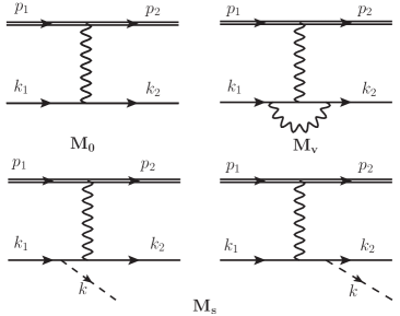
Let us consider the model-independent QED radiative corrections which are due to the vacuum polarization and emission of the virtual and real (soft and hard) photons in the electron vertex. The corresponding diagrams are shown in Fig. 1.
III.1 Soft photon emission
In this section we give the expressions for the contribution to the radiative corrections of the soft photon emission when the photons are emitted by the initial and final electrons
| (21) |
The matrix element in this case (the photon emitted from the electron vertex) is given by
| (22) |
where the electron current corresponding to the photon emission is
| (23) |
where is the polarization four vector of the emitted photon and .
The differential cross section of reaction (21) can be written as
| (24) |
It is necessary to integrate over the photon phase space. Since the photons are assumed to be soft, then the integration over the photon energy is restricted to . The quantity is determined by particular experimental conditions and it is assumed that is sufficiently small to neglect the momentum in the function and in the numerators of the matrix element of the process (21). In order to avoid the infrared divergence, which occurs in the soft photon cross section, a small fictitious photon mass is introduced.
The differential cross section of the process (21), integrated over the soft photon phase space, can be written as
| (25) |
where the radiative correction due to the soft photon emission is
| (26) | |||||
where is the Spence (dilogarithm) function defined as
III.2 Virtual photon emission
In this section, we give the expressions for the contribution to the radiative corrections of the virtual photon emission in the electron vertex (the electron vertex correction) and the vacuum polarization term.
As we limit ourselves to the calculation of the radiative corrections at the order of in comparison with the Born term, it is sufficient to calculate the interference of the Born matrix element with
| (27) |
where the term is due to the modification of the term in the electron vertex, and the term is due to the presence of the structure in the electron vertex.
The radiative corrections due to the emission of the virtual photon in the electron vertex can be written as
| (28) | |||||
| (29) |
The radiative correction due to the vacuum polarization is (the electron loop has been taken into account):
| (30) |
For small and large values of the variable we have
Taking into account the radiative corrections given by Eqs. (26, 29, 29, 30), we obtain the following expression for the differential cross section:
| (31) |
where the radiative corrections and are given by
| (32) | |||||
We separate the contribution since it can be summed up in all orders of the perturbation theory using the exponential form of the electron structure functions KF85 . To do this it is sufficient to keep only the exponential contributions in the electron structure functions. The final result can be obtained by the substitution of the term by the following term
| (33) |
where
III.3 Hard photon emission
In this section we calculate the radiative correction due to the hard photon emission (with the photon energy ) from the initial and recoil electrons only (the model-independent part). The contribution due to radiation from the initial and scattered deuterons (the model-dependent part) requires a special consideration and we leave it for other investigations. We consider the experimental setup when only the energies of the scattered deuteron and final electron are measured.
The differential cross section of the reaction (21), averaged over the initial particle spins, can be written as
| (34) |
where and the leptonic tensor has the following form
| (35) |
The hadronic tensor is defined by Eqs. (15 ,16) with the substitution The contraction of the leptonic and hadronic tensors reads
| (36) |
where the functions have the following expressions
| (37) |
| (38) | |||||
Integrating over the scattered deuteron variables we obtain the following expression for the differential cross section
| (39) |
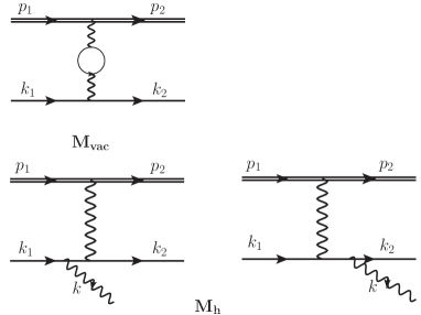
To integrate further we have to define the coordinate system. Following Ref. K64 , where the scattering has been analyzed, let us take the -axis along the vector and the momenta of the initial deuteron and emitted photon lie in the plane. The momentum of the scattered electron is defined by the polar and azimuthal angles as it is shown in Fig. 2. The angle is the angle between the beam direction and axis (emitted photon momentum).
Integrating over the polar angle of the scattered electron we obtain:
| (40) |
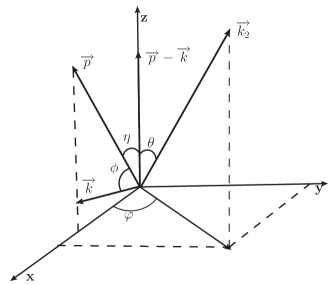
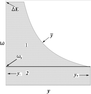
The region of allowed photon momenta should be determined. The experiment counts those events which, within the accuracy of the detectors, are considered ”elastic”. We refer to the experimental situation where the energies of the scatted deuteron and recoil electron are measured. Because of the uncertainties in determination of the recoil electron () and scattered deuteron () energies, which are usually proportional to and respectively, the elastic deuteron-electron scattering is always accompanied by hard photon emission with energies up to . For deuteron beam energies of the order of 100 GeV this value can reach a few GeV. The events corresponding to scattered deuteron energy and recoil electron energy (they satisfy the condition ) are considered as true elastic events. Here, and are the uncertainties of the measurement of the final deuteron and recoil electron energies. The plot of the variable versus the variable is shown in Fig. 3. The shaded area in this figure represents the region where events are allowed by the experimental limitations. The relation between the energies and , as it is shown in Fig. 3, has to be transformed into a limit on the possible photon momentum .
As we already mentioned, usually the uncertainties and are proportional to and respectively. For the deuteron beam energies up to 500 GeV, the recoil electron energy is about two orders of magnitude smaller than the scattered deuteron one. Therefore, holds and the effect due to nonzero value of is negligible. In our further numerical calculations we take
We consider the experimental setup where no angles are measured and, therefore, the orientation of the photon momentum is not limited and investigate both cases: i) and ii) , where and is defined by Eq. (5).
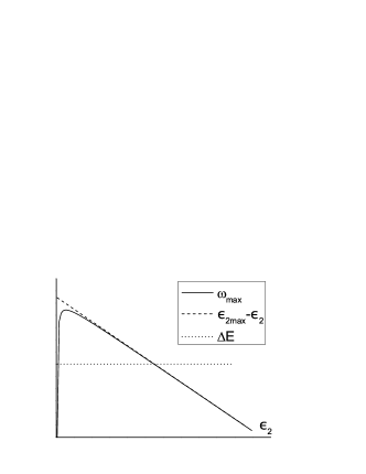
In the first case we get, as experimental limit, the isotropic condition whereas in the second case the upper limit of depends on the recoil electron energy as it is shown in Fig. 4.
Note that quantity is the root of the equation and has the following form
| (41) |
In the chosen coordinate system the element of solid angle becomes: . We introduce a new variable and rewrite Eq. (40) as
| (42) |
where the integration region over the variables and for the case is shown in the left panel of Fig. 5, and
| (43) |
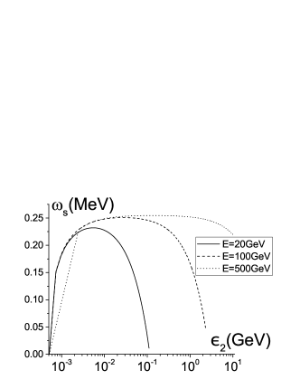
The quantity represents the maximal energy, when the photon can be emitted in the whole angular phase space. The dependence of this quantity on the recoil electron energy, at different values of the deuteron beam energy, is shown in the right panel of Fig.5. We see that it is of the order of the electron mass in a wide range of the energies and . Because our analytical calculations for the soft photon correction were performed under the condition where is the maximal energy of the soft photon, we can not identify with as it has been done in the paper K64 .
So, the expression for the cross section given by Eq. (42) can be written as a sum of two terms
| (44) |
where
| (45) |
.
The scalar products of various 4-momenta, which enter in the expressions for and , are expressed, in terms of the angles, as illustrated in Fig. 2, and the photon energy, as follows:
| (46) |
In turn, the respective trigonometric functions of angles are expressed through the photon energy and the variable as:
| (47) |
The functions and depend on the azimuthal angle , and, in order to perform the integration over this variable in the r.h.s. of Eq. (44), one needs to use a specific expressions for the form factors entering these functions. Further we concentrate on small values of the squared momentum transfer as compared with the deuteron mass, where the form factors can be expanded in a series in term of powers of In the calculations we keep the terms of the order of , and in the quantity
which enters the differential cross section.
The integration in the r.h.s. of Eq. (44) over the and variables is performed analytically. The result for both and is very cumbersome, and it will be published elsewhere. In the limit the function is regular, and the function has an infrared behavior. We extract the regular part and the infrared contribution by a simple subtraction procedure,according to
| (48) |
The infrared contribution is combined with the correction due to soft and virtual photon emission. This results in the substitution in the expression for , see Eq. (III.2). The integration of the regular part over (we can chose an arbitrary small value as the lower limit) as well the whole contribution of the region 1, is performed numerically.
IV Numerical estimations and discussion
In this section, the conditions for the experimental uncertainties are set to and the parametrization of the deuteron form factors is taken as below, if no other choice is specified.
In our calculation we use four different parameterizations of the deuteron form factors, and since the four-momentum transfer squared is rather small in this reaction, we can approximate these form factors by a Taylor series expansion with a good accuracy. On the Born level and when calculating the virtual corrections we can use also unexpanded expressions, but, in order to perform the analytical integrations in Eq. (45), we have to expand the differential cross section keeping terms up to in and .
So, we use the expansion over the variable of the following four form factor parameterizations.
By means of the radii (labeled as ”rad ”). In this approach we expand the quantity which is defined by Eq. (18), including terms up to and we use the expansion of the form factors taking into account only the mean square charge and magnetic radii from Ref. S01 .
| (49) |
”Two-component model for the deuteron electromagnetic structure” TGA06 (labeled as ”m”). In this approach the deuteron form factors are saturated by contribution of the isoscalar vector mesons, and In this case one can write:
| (50) |
with:
where () is the mass of the ()-meson. Note that the dependence of is parameterized in such form that , for any values of the free parameters and , which are real numbers.
The terms are written as functions of two real parameters, and , generally different for each form factor:
| (51) |
and is the normalization of the -th form factor at :
where , and are the quadrupole and the magnetic moments of the deuteron.
The experimental data for and show the existence of a zero, for GeV2 and GeV2. The requirement of a node gives the following relation between the parameters and , and :
| (52) |
The expression (50) contains four parameters, , , , , generally different for different form factors. The values of the best fit parameters are reported in Table 1. The common parameters are , , corresponding to In our calculations we used the central values of this parameters.
”Deuteron Electromagnetic Form Factors in the Transition Region Between Nucleon-Meson and ”
Quark-Gluon Pictures KS94 (labeled as ”k”). In this approach, form factors are consistent with the results from popular NN-potentials at low energies ( 1(GeV/c)2), but, at the same time, they provide the right asymptotic behavior following from quark counting rules, at high energies ( 1(GeV/c)2). The explicit expressions of the deuteron form factors are:
| (53) |
where is some parameter of order of the nucleon mass. The functions , , and have the following parametrization:
where are fitting parameters. From the quark counting rules it follows that the fall-off behavior of these amplitudes at high is
which, together with the requirement of a correct static normalization, impose the set of constraints on :
| (54) |
In our calculations we used the following sequence for each group of these parameters:
(similarly, for and ), where and have the dimension of energy. The parameters are listed in Table 2 for n=4.
| 1 | 2 | 3 | 4 | |
| see (54) | ||||
| see (54) | see (54) | |||
| see (54) | see (54) | see (54) | ||
”Jefferson collaboration” (labeled as ) A2000 . The three deuteron electromagnetic form factors have been determined by fitting directly the all existing measured differential cross section and polarization observables, according to the following expressions:
| (55) |
where
The parameters have such dimensions of the inverse powers to quantities were dimensionless. The values of these parameters appear in Table 3 with in fm2 units.
| 1 | 2 | 3 | 4 | 5 | |
|---|---|---|---|---|---|
| 0.674 | 0.02246 | 0.009806 | -0.0002709 | 0.000003793 | |
| 0.5804 | 0.08701 | -0.003624 | 0.0003448 | -0.000002818 | |
| 0.8796 | -0.5656 | 0.01933 | -0.0006734 | 0.000009438 |
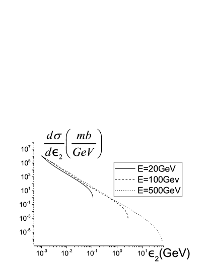
To illustrate the dependence of the recoil electron distribution on the deuteron beam energy, the Born cross section is shown in Fig. 6 for standard parametrization at E=20 GeV, 100 GeV and 500 GeV. Here and below, for the beam energy 500 GeV we limi the recoil electron energy to 10 GeV, because for largest values the expansions for the form factors are incorrect.
The sensitivity of this cross section to different form factor parameterizations is shown in Fig. 7, in terms of the quantities (in percentages)
| (56) |
where is the differential cross section (17), and i=k, m, rad, correspond to the above-mentioned deuteron form factors. As one can see, the sensitivity has a very similar behaviour for the expanded and unexpanded cross sections and increases when both the deuteron and recoil electron energies increase. However, the differential cross section decreases very quickly when the recoil electron energy increases (see Fig. 6).

The hard photon correction depends on the parameter due to the contribution of the region 1 in Fig. 5 (left panel). To illustrate this dependence, we show in Fig. 8 the quantity (in which the contribution of the region 2 is removed)
| (57) |
as a function of the recoil electron energy for the parametrization. The effect is rather small: on the level for E=500 (100) GeV. If the deuteron energy is 500 GeV (lower row) this dependence exhibits the monotonic increase with the recoil electron energy, whereas at the energy 100 GeV (upper row) it has maximum and then decreases up to zero. In this zero-point, the recoil-electron energy value is the root of the equation provided that line in Fig. 4 lies above the curve At the deuteron energy 500 GeV this last condition is not fulfilled.


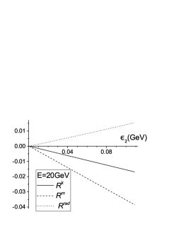
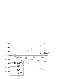
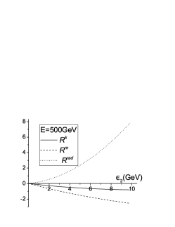
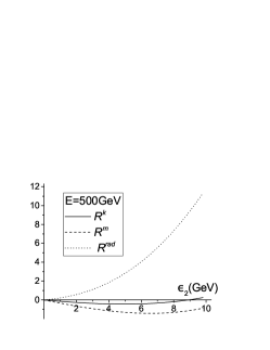
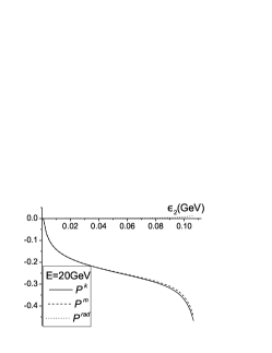
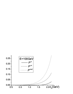
In Fig. 9 we present the quantities and defined as
| (58) |
which we call ”modified hard and soft and virtual corrections”, respectively, as well their sum that is the total model-independent first order radiative correction (the last term in is :
Note, that both modified corrections in Eq. (IV) are independent on the auxiliary parameter but depend on the physical parameter and, therefore, have a physical sense.
To calculate we can write the quantity using the expression (III.2) or its exponential form defined by (33) (with substitution ). But numerical estimations show that they differ very insignificantly, by a few tenth of the percent, and further we do not use the exponential form.
We see that at small values of the squared momentum transfer (small recoil-electron energy ) the total model-independent radiative correction is positive and it decreases (with increase of ), reaching zero and becoming negative. The absolute value of the radiative correction does not exceed 6 although the strong compensation of the large (up to 30 %) positive ”modified hard” and negative ”modified soft and virtual” corrections takes place. Such behavior of the pure QED correction is similar to one derived in Ref. K64 .
If the deuteron form factors are determined independently with high accuracy from other experiments, the measurement of the cross section can be used, in principle, to measure the model-dependent part of the radiative correction in the considered conditions. This possibility is similar to the one described in Ref. Abbiendi:2017 where the authors proposed to determine the hadronic (model-dependent) contribution to the running electromagnetic coupling by a precise measurement of the differential cross section, assuming that QED model-independent radiative corrections are under control.


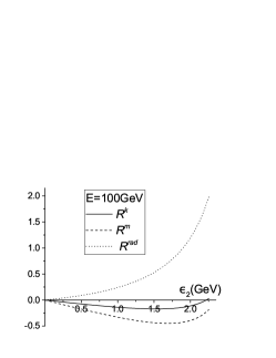
In Fig. 10 we illustrate the sensitivity of the total radiative correction to the parametrization of the form factors in terms of the ratios
| (59) |
where is the total correction for standard fit. We see that, in the considered conditions, the deviation of these quantities from unity is very small. We conclude that the influence of the parameterizations of the form factors on the radiative corrections is much smaller than on the Born cross section.

V Conclusion
In this paper we investigated the recoil-electron energy distribution in elastic deuteron-electron scattering in a coincidence experimental setup, taking into account the model-independent QED radiative corrections. The detection of the recoil electron in this process, with energies from a few MeV up to 10 GeV, allows to collect small- data, at 10-5 GeV2 10-2 GeV Such data, being combined with the existing and future experiments with electron beams, will give precise information on the small- behavior of the deuteron electromagnetic form factors. This allows to reach a meaningful extrapolation to the static point and to extract the deuteron charge radius.
To cover the above mentioned interval of -values, it is desirable to use the deuteron beams with quite large energies, of the order of a few hundreds GeV. The sensitivity of the differential cross section to the form factors parameterizations, labeled as k, m, and 20, is small (does not exceed 2 ), but the rad-parametrization gives a value of the cross section about 10 smaller as compared with the 20-parametrization at 10-2 GeV2 (see Fig. 7).
We took into account the first order QED corrections due to the vacuum polarization and the radiation of the real and virtual photons by the initial and final electrons, paying special attention to the calculation of the hard photon emission contribution when the final deuteron and electron energies are determined. This hard radiation takes place due to the uncertainty in the measurement of the deuteron (electron) energy, . In our calculations we follow Ref. K64 for the choice of the coordinate system and the angular integration method. Analytical expressions for the functions and defined by Eq. (45) can be reconstructed using the corresponding results for the protonelectron scattering which were previously published GKM17 . The cancellation of the auxiliary infrared parameter in the sum of the soft and hard corrections was performed analytically and the remaining integration in (44) was done numerically.
We assumed that uncertainties in the final particle energies are proportional to their energies and we showed that the effect due to the nonzero quantity is negligible.
As usual, there is a strong cancellation between the positive hard correction and negative virtual and soft ones, as it is seen in Fig. 9. Despite the fact that the absolute values of these corrections reach separately 20 30, their sum does not exceed 6 at E=20 GeV and 100 GeV and 3.5 at E=500 GeV for the value and the -parametrization used in these calculations.
The total correction shows a weak dependence on the form factors parametrization in the considered region (see. Fig. 10). At the lower values of , which correspond to the lower values of the recoil electron energy the total correction is positive and changes sign when increases. Such behaviour of is similar to the one found in Ref. K64 and confirmed in Ref. Bardin:1969 for the case of pion electron scattering.
In our earlier work GKMT about proton-electron scattering we have estimated also the model-dependent part of radiative correction and found that it cannot affect the experimental cross sections measured within 0.2 accuracy. We expect that in the case of the deuteron-electron scattering it is even less essential because the deuteron mass is two times larger.
Thus, we conclude that the model-independent part of the radiative corrections are under control and, if necessary, it can be calculated with a more high accuracy. We believe also that the uncertainty due to its model-dependent part in the considered region is negligible.
Acknowledgments
This work was partially supported by the Ministry of Education and Science of Ukraine (projects no. 0115U000474 and no. 0117U004866). The research is conducted in the scope of the IDEATE International Associated Laboratory (LIA).
References
- (1) S. Pacetti, R. Baldini Ferroli, and E. Tomasi-Gustafsson, Phys. Rep. 550-551, 1(2015).
- (2) C. Perdrisat, V. Punjabi, and M. Vanderhaeghen, Prog.Part.Nucl.Phys. 59, 694 (2007), arXiv:hep-ph/0612014 [hep-ph].
- (3) A. Antognini et al., Science 339, 417 (2013).
- (4) P. J. Mohr, D. B. Newell, and B. N. Taylor, Rev. Mod. Phys. 88, 035009 (2016).
- (5) A. Antognini et al., J. Phys. Conf. Ser. 312, 032002 (2011).
- (6) I. Sick, Prog. Part. Nucl. Phys. 47, 245 (2001).
- (7) R. A. Gilman and F. Gross, J. Phys. G28, R37 (2002).
- (8) F. Gross, Eur. Phys. J. A17, 407 (2003).
- (9) Cuiying Liang, Yubing Dong, and Weihong Liang, arXiv:1406.2523v1 [hep-ph].
- (10) N. G. Kelkar and D. Bedoya Fierrj, arXiv:1610.07498v1 [nucl-th].
- (11) R. Pohl et al., Science 353, 669 (2016).
- (12) P. J. Mohr, B. N. Taylor, D. B. Newell, Rev. Mod. Phys. 84, 1527 (2012).
- (13) Randolf Pohl et al., Deuteron charge radius and Rydberg constant from spectroscopy data in atomic deuterium, arXiv:1607.03165V2 [physics.atom-ph].
- (14) I. V. Glavanakov, Yu. F. Krechetov, A. P. Potylitsyn, G. M. Radutsky, A. N. Tabachenko and S. B. Nurushev, Nucl. Instrum. Meth. A 381 (1996) 275; I. V. Glavanakov, Yu. F. Krechetov, G. M. Radutskii and A. N. Tabachenko, JETP Lett. 65 (1997) 131 [Pisma Zh. Eksp. Teor. Fiz. 65 (1997) 123].
- (15) G. I. Gakh, A. Dbeyssi, D. Marchand, E. Tomasi-Gustafsson, V. V. Bytev, Phys.Rev. C84, 015212 (2011).
- (16) G. I. Gakh, A. Dbeyssi, E. Tomasi-Gustafsson, D. Marchand, V. V. Bytev, Phys.Part.Nucl.Lett. 10, 393 (2013).
- (17) G. I. Gakh, M.I. Konchatnij, N.P. Merenkov, Egle Tomasi-Gustafsson, Phys.Rev. C95, 055207 (2017).
- (18) Rene Reifarth and Yuri A. Litvinov, arXiv:1312.3714v1 [nucl-ex].
- (19) E. Kuraev and V. S. Fadin, Sov. J. Nucl. 41, 466 (1985).
- (20) J. Kahane, Phys. Rev. B135, 975 (1964).
- (21) E. Tomasi-Gustafsson, G. I. Gakh, and C. Adamuščin, Phys. Rev. C73, 045204 (2006).
-
(22)
A. P. Kobushkin and A. I. Syamtomov, Phys. At. Nucl. 58, 1477
(1995)[Yad. Fiz. 58, 1565 (1995)];
arXiv:9409.411v1 [hep-ph]. - (23) D. Abbott et al., Eur. Phys. J. A 7, 421 (2000).
- (24) G. Abbiendi et al., Eur. Phys. J. C 77, 139 (2017).
- (25) G.I. Gakh, M.I. Konchaynij, N.P. Merenkov, Egle Tomasi-Gustavsson, arXiv:1612.02139; [hep-ph].
- (26) D.Y. Bardin, V.B. Semikoz, and N.N. Shumeiko, Yad. Fiz. 10, 1020 (1969).