The effect of forcing on vacuum radiation

Abstract

Vacuum radiation has been the subject of theoretical study in both cosmology and condensed matter physics for many decades. Recently there has been impressive progress in experimental realizations as well. Here we study vacuum radiation when a field mode is driven both parametrically and by a classical source. We find that in the Heisenberg picture the field operators of the mode undergo a Bogolyubov transformation combined with a displacement; in the Schrödinger picture the oscillator evolves from the vacuum to a squeezed coherent state. Whereas the Bogolyubov transformation is the same as would be obtained if only the parametric drive were applied the displacement is determined by both the parametric drive and the force. If the force is applied well after the parametric drive then the displacement is the same as would be obtained by the action of the force alone and it is essentially independent of $t_{f}$, the time lag between the application of the force and the parametric drive. If the force is applied well before the parametric drive the displacement is found to oscillate as a function of $t_{f}$. This behavior can be understood in terms of quantum interference. A rich variety of behavior is observed for intermediate values of $t_{f}$. The oscillations can turn off smoothly or grow dramatically and decrease depending on strength of the parametric drive and force and the durations for which they are applied. The displacement depends only on the Fourier component of the force at a single resonant frequency when the forcing and the parametric drive are well separated in time. However for a weak parametric drive that is applied at the same time as the force we show that the displacement responds to a broad range of frequencies of the force spectrum. Implications of our findings for experiments are briefly discussed.

1 Introduction

In a landmark paper, Casimir recognized that quantum vacuum fluctuations can produce measurable effects, for example, an attractive force between two parallel conducting plates in a vacuum casimir . Subsequently, Moore moore observed that motion of the conducting plates would result in the generation of radiation from the vacuum, an effect dubbed the dynamical Casimir effect. Earlier, Parker parker showed that in an expanding Universe, vacuum fluctuations would lead to particle production; according to the modern inflationary paradigm this mechanism is the origin of structure in the Universe weinberg . In his seminal work, Hawking hawking showed that even an apparently static system such as a non-rotating black hole will produce vacuum radiation due to its horizon. More recently, there have been significant advances on the experimental front: the Casimir effect casimirexpt and the dynamical Casimir effect superconduct have been unambiguously observed, and a laboratory analog of Hawking radiation proposed by Unruh unruh has been claimed to have been observed in a Bose-Einstein condensate bec .

A common element in much analysis of dynamical Casimir radiation is to assume that the system starts in the vacuum state. However in cosmology there is an ambiguity about what constitutes the appropriate initial state and hence there has been an exploration of various alternative vacua as the initial state bunch . Still earlier, in context of Hawking radiation from black holes, Wald explored the consequences of starting the system in an excited state rather than the vacuum. He found that the quantum radiation was enhanced in a manner reminiscent of stimulated emission wald . Here we wish to study the related but distinct effect of starting the system in the vacuum and examining the quantum radiation that results when the system is simultaneously excited parametrically (as in the dynamical Casimir effect) and also driven directly by a classical source. This analysis may be relevant to the experimental systems that are currently under investigation noted above and discussed further in section 4. Another key motivation for this work is the observation of gravitational radiation from merging black holes ligo . The gravitational radiation in this case is predominantly classical and reliable calculation of its magnitude has only recently been achieved numerics . In order to estimate the quantum contribution to radiation in a merger it would be necessary to take into account the strong classical driving to which the gravitational radiation field is subject in these events. Here for simplicity we primarily focus on a simple toy model of a single field mode. In section 2.4 we sketch the generalization to coupled modes and a complete field theory.

We assume that the oscillator experiences parametric driving (frequency $\omega$ varies in time approaching the natural value $\omega_{0}$ asymptotically for $t\rightarrow\pm\infty$) and in addition an applied force $F(t)$. When treated individually the effect of each is well-known: in the Heisenberg picture, for a parametrically-driven oscillator the evolution of the ladder operators is a Bogolyubov transformation, and for a forced oscillator the ladder operators undergo simple displacement. Equivalently in the Schrödinger picture the vacuum evolves into a squeezed vacuum state under parametric driving and into a coherent state under forcing. Our principal finding is that when the oscillator is driven parametrically as well as by a force then in the Heisenberg picture the ladder operators undergo a Bogolyubov transformation combined with a displacement (see eq (15)), or equivalently, in the Schrödinger picture the vacuum evolves to a squeezed coherent state.

Furthermore, whereas the Bogolyubov transformation is found to be exactly the same as it would be in the absence of forcing, the displacement is markedly influenced by the simultaneous application of forcing and parametric driving. Only if the force is applied well after the parametric drive is the displacement the same as would have been obtained in the absence of the parametric drive. If the force is applied well before the parametric drive, the final state is the same as one would obtain if only the parametric drive were applied but the starting state was an appropriately chosen coherent state rather than the vacuum. When the parametric drive is applied at the same time as the force (the case of primary interest here) it has a dramatic effect on the displacement.

The behavior the displacement $\alpha$ as a function of the time lag between the force and the parametric drive $t_{f}$ is shown in fig 1. We show generically that for $t_{f}\rightarrow-\infty$ (force is applied much earlier than the parametric drive) $|\alpha|$ should undergo oscillations due to quantum interference; for $t_{f}\rightarrow\infty$ (force is applied much later than the parametric drive) the displacement should approach a constant value controlled by the Fourier component of the force at the frequency $\omega_{0}$. A rich variety of behavior is seen at intermediate $t_{f}$. We find in the adiabatic limit (slowly varying $\omega(t)$) the oscillations turn off with a profile that may be described by a complementary error function. In the opposite abrupt limit too the oscillations turn off smoothly and monotonically (fig 1 lower panel). However for other values of the parameters using an exactly soluble model we find that the oscillations can grow dramatically even when they are negligible for $t_{f}\rightarrow-\infty$ (fig 1 upper panel). The displacement depends only on the Fourier component of the force at frequency $\omega_{0}$ in the absence of parametric driving or when the parametric drive and the force are well separated in time; however when the parametric drive is weak and applied at the same time as the force we are able to show perturbatively that the displacement responds to a broad range of frequencies in the driving force.

The remainder of this paper is organized as follows. In section 2 we present a general analysis of the model. We show that in the Heisenberg picture the field operators will undergo a Bogolyubov transformation combined with a displacement and derive general formulae for the transformation parameters and the displacement. We interpret these results in the Schrödinger picture and extend the general analysis to multiple coupled modes and field theory. In section 3 we return to a single mode and analyze a soluble model and various approximations that illustrate the rich variety of behavior that is obtained due to the interplay of the forcing and the parametric drive. In section 4 we discuss the implications of our results for experiments and open questions.

2 Forced oscillator: general analysis

We consider a harmonic oscillator of mass $m$ whose natural frequency $\omega(t)$ varies in time; the time variation of the frequency represents the parametric driving that leads to vacuum radiation. The frequency is assumed to approach the natural value $\omega_{0}$ asymptotically as $t\rightarrow\pm\infty$. In addition the oscillator also experiences a time dependent force $F(t)$ that is also assumed to vanish asymptotically as $t\rightarrow\pm\infty$; the forcing corresponds to a classical source that drives the field. For the applications we envisage the oscillator represents a single mode of a quantum field that is in some approximation decoupled from other degrees of freedom. Generally we will assume that the oscillator starts in the vacuum state $|0\rangle$ which is well defined as $t\rightarrow-\infty$ and we wish to determine the final behavior of the system as $t\rightarrow\infty$. Throughout the paper we adopt units where $\hbar=1$.

2.1 Classical Analysis

It is helpful to first solve the classical equation of motion

$$\frac{d^{2}x}{dt^{2}}+\omega^{2}(t)x=\frac{F(t)}{m}.$$ (1)

For the case $F=0$ eq (1) has the form of a Schrödinger equation for a particle scattering from a localized potential. Thus we can draw upon our intuition about the Schrödinger equation to deduce that there exists a solution with asymptotic behavior

$$\xi(t) \rightarrow e^{-i\omega_{0}t}\hskip 8.53581pt{\rm for}\hskip 8.53581ptt\rightarrow-\infty$$ (2)

$$\rightarrow Ae^{-i\omega_{0}t}+Be^{i\omega_{0}t}\hskip 8.53581pt{\rm for}\hskip 8.53581ptt\rightarrow\infty$$

where $A$ and $B$ are scattering coefficients. Since eq (1) is real $\xi^{\ast}(t)$ constitutes a second independent solution. Note that these solutions have been chosen to satisfy Jost boundary conditions which are more suitable for our purpose than the conventional scattering boundary conditions. It is evident from the Schrödinger analogy that

$$|A|^{2}-|B|^{2}=1.$$ (3)

In section 3 we solve eq (1) approximately in various circumstances and exactly for a particular choice of $\omega^{2}(t)$ and thereby obtain more explicit expressions for the coefficients $A$ and $B$ and for $\xi(t)$.

It is easy to verify that the solution that flows from the initial conditions $x(t_{0})=x_{0}$ and $p(t_{0})=p_{0}$ is

$$\overline{x}(t) = \frac{1}{2}\left(x_{0}+i\frac{p_{0}}{m\omega_{0}}\right)e^{i\omega_{0}t_{0}}\xi(t)$$

$$+ \frac{1}{2}\left(x_{0}-i\frac{p_{0}}{m\omega_{0}}\right)e^{-i\omega_{0}t_{0}}\xi^{\ast}(t).$$

Here we have assumed that $t_{0}$ is far in the past before the parametric drive was turned on. Eq (LABEL:eq:xsolution) can be further simplified if we assume that $t$ is sufficiently far in the future that the parametric drive has been turned off. In that case we can use the $t\rightarrow\infty$ asymptotic form of $\xi(t)$ given in eq (2). By differentiating eq (LABEL:eq:xsolution) one can then obtain $\overline{p}(t)$, the momentum for the solution that flows from the initial conditions $(x_{0},p_{0})$.

In order to analyze the effects of the force it is helpful to first consider the response $g(t,\tau)$ to an impulse $F(t)/m=\delta(t-\tau)$ at time $\tau$. With the retarded boundary condition $g(t,\tau)=0$ for $t<\tau$ the impulse response is given by

$$g(t,\tau)=\frac{\theta(t-\tau)}{W}\left[\xi(\tau)\xi^{\ast}(t)-\xi^{\ast}(\tau)\xi(t)\right]$$ (5)

where $\theta$ is the unit step function. The Wronskian $W=\xi(t)\xi^{\ast}$${}^{\prime}(t)-\xi^{\prime}(t)\xi^{\ast}(t)$, where primes denote differentiation with respect to $t$. Since the Wronskian is a constant independent of time we use the $t\rightarrow-\infty$ behavior of $\xi$ to obtain $W=2i\omega_{0}$.

Now by superposition the solution that flows from the initial condition $x(t_{0})=x_{0}$ and $p(t_{0})=p_{0}$ is given by

$$x(t)=\overline{x}(t)+\frac{1}{m}\int_{t_{0}}^{t}d\tau\;g(t,\tau)F(\tau).$$ (6)

Here we assume that $t_{0}$ is far in the past before either the force or the parametric drive turn on. By differentiating eq (6) we then obtain the momentum $p(t)$ that flows from the initial conditions $(x_{0},p_{0})$ under the influence of both the force and the parametric drive.

Eqs (LABEL:eq:xsolution) and (6) represent the solution to eq (1) for a given initial condition. From the classical solution it is now easy to construct a complete solution to the corresponding quantum problem as discussed below.

2.2 Heisenberg picture

We turn now to the quantum problem. The quantum Hamiltonian corresponding to our model is

$$\hat{H}=\frac{1}{2m}\hat{p}^{2}+\frac{1}{2}m\omega^{2}(t)\hat{x}^{2}-F(t)\hat{x}.$$ (7)

This leads to the Heisenberg equations of motion

$$\frac{d}{dt}\hat{x}=\frac{1}{m}\hat{p},\hskip 8.53581pt\frac{d}{dt}\hat{p}=-m\omega^{2}(t)\hat{x}+F(t).$$ (8)

First for simplicity let us assume $F=0$. Because of their linearity the solution to the quantum Heisenberg equations of motion can be constructed using the classical solution eq (LABEL:eq:xsolution). We obtain

$$\hat{x}(t) = \frac{1}{2}\left(\hat{x}_{0}+i\frac{\hat{p}_{0}}{m\omega_{0}}\right)e^{i\omega_{0}t_{0}}\xi(t)$$

$$+ \frac{1}{2}\left(\hat{x}_{0}-i\frac{\hat{p}_{0}}{m\omega_{0}}\right)e^{-i\omega_{0}t_{0}}\xi^{\ast}(t)$$

and an analogous relation that expresses $\hat{p}(t)$ in terms of $\hat{x}_{0}$ and $\hat{p}_{0}$ from the classical expression for $\overline{p}(t)$. It is easy to verify that these expressions for $\hat{x}(t)$ and $\hat{p}(t)$ satisfy the Heisenberg equations of motion and the appropriate initial conditions $\hat{x}(t_{0})=\hat{x}_{0}$ and $\hat{p}(t_{0})=\hat{p}_{0}$.

For the quantum oscillator it is preferable to work with the creation operator $\hat{a}=\sqrt{m\omega/2}(\hat{x}+i\hat{p}/m\omega)$ and the annihilation operator $\hat{a}^{\dagger}$. From the evolution of $\hat{x}$ and $\hat{p}$ we find

$$\hat{a}(t)=u\hat{a}_{0}+v\hat{a}^{\dagger}_{0}\hskip 8.53581pt{\rm and}\hskip 8.53581pt\hat{a}^{\dagger}(t)=u^{\ast}\hat{a}_{0}^{\dagger}+v^{\ast}\hat{a}_{0}.$$ (10)

Thus the evolution of the ladder operators is a Bogolyubov transformation with coefficients

$$u=A\exp[-i\omega_{0}(t-t_{0})] \hskip 5.69054pt{\rm and}\hskip 5.69054pt v=B^{*}\exp[-i\omega_{0}(t+t_{0})]$$

In eqs (10) and (LABEL:eq:bcoefficients) we have assumed that $t_{0}$ is well before the parametric drive turns on and $t$ is well after.

If we assume that the initial state of the system at $t_{0}$ is the vacuum $|0\rangle$ defined by $a_{0}|0\rangle=0$ then in the Heisenberg picture of quantum mechanics the number of quanta excited at time $t$ is given by

$$\langle 0|\hat{a}^{\dagger}(t)\hat{a}|0\rangle=|B|^{2}.$$ (12)

This excitation of the system is the basic phenomenon of vacuum radiation. Suppose following wald we assume that the initial state of the system already has $n$ quanta then

$$\langle n|\hat{a}^{\dagger}(t)\hat{a}(t)|n\rangle-\langle n|\hat{a}^{\dagger}_{0}\hat{a}_{0}|n\rangle=(2n+1)|B|^{2}.$$ (13)

This enhancement over the $n=0$ result is a special case of the stimulated emission of vacuum radiation described by wald . Another interesting initial state to consider is a coherent state $|\alpha\rangle$ defined by $\hat{a}_{0}|\alpha\rangle=\alpha|\alpha\rangle$ with $\alpha$ the complex coherent amplitude. In this case we obtain

$$\langle\alpha|\hat{a}^{\dagger}(t)\hat{a}(t)|\alpha\rangle-\langle\alpha|\hat{a}^{\dagger}_{0}\hat{a}_{0}|\alpha\rangle = (2|\alpha|^{2}+1)|B|^{2}$$

$$+ 2|A||B||\alpha|^{2}\cos(2\omega_{0}t_{0}+2\phi).$$

Here the phase $\phi$ is defined by the relation $\alpha^{2}AB=|\alpha|^{2}|A||B|e^{i2\phi}$. Once again the first term on the right hand side corresponds to an enhancement compared to the excitation of the vacuum $|0\rangle$ which is simply a coherent state with $\alpha=0$. The second term shows a remarkable oscillatory behavior in time due to quantum interference. Due to the Heisenberg dynamics the number of quanta is uncertain at the final time even if it is definite initially; the interference is between states with differing numbers of quanta present. We will see that this oscillatory behavior occurs under many conditions when the oscillator is forced even if the initial state is the vacuum.

Now let us include the force $F$ in our analysis. Once again the solution to the quantum Heisenberg equations of motion can be constructed by adapting the classical solution eq (6) and its counterpart for $p(t)$. Again it is preferable to work with the creation and annihilation operators $\hat{a}$ and $\hat{a}^{\dagger}$ rather than $\hat{x}$ and $\hat{p}$. The final result is

$$\hat{a}(t)=u\hat{a}_{0}+v\hat{a}_{0}^{\dagger}+\alpha\hskip 8.53581pt{\rm and}\hskip 8.53581pt\hat{a}^{\dagger}(t)=u^{\ast}\hat{a}_{0}^{\dagger}+v^{\ast}\hat{a}_{0}+\alpha^{\ast}.$$ (15)

Thus the evolution of the ladder operators in this case is a Bogolyubov transformation together with a constant displacement $\alpha$. The coefficients $u$ and $v$ are still given by eq (LABEL:eq:bcoefficients) assuming that $t_{0}$ is before the force or parametric drive are turned on and $t$ is after. The displacement $\alpha$ is given by

$$\alpha=\frac{ie^{-i\omega_{0}t}}{\sqrt{2m\omega_{0}}}\int_{t_{0}}^{t}d\tau\;F(\tau)[A\;\xi^{\ast}(\tau)-B^{\ast}\xi(\tau)].$$ (16)

It is useful to consider various special cases of this result. First suppose that there is no parametric driving. In that case $A=1$ and $B=0$ and $\xi(\tau)=\exp(-i\omega_{0}\tau)$ for all time. Hence in this case

$$\alpha=\frac{ie^{-i\omega_{0}t}}{\sqrt{2m\omega_{0}}}\tilde{f}(\omega_{0})e^{i\omega_{0}t_{f}}$$ (17)

and the number of quanta at time $t$ is given by $\langle 0|\hat{a}^{\dagger}(t)\hat{a}|0\rangle=|\alpha|^{2}$. Here we have taken the force to be $f(t-t_{f})$ in the time domain. The force is assumed to be localized about the time $t_{f}$. For explicit calculations below we will sometimes take the force to be a Gaussian centered at $t_{f}$ with a sinusoidal modulation. Thus we arrive at the well-known result loudon ,landaucm that the excitation of the field oscillator is determined by $\tilde{f}(\omega_{0})$, the Fourier amplitude of the force at the natural frequency of the mode, $\omega_{0}$. In the Schrödinger picture the state of the oscillator evolves from the vacuum $|0\rangle$ to the coherent state $|\alpha\rangle$.

Next suppose that the force is applied well before the parametric drive. In that case we can use the $t\rightarrow-\infty$ behavior of $\xi(t)$ in order to evaluate $\alpha$. Making use of eq (2) and 16) we obtain

$$\alpha\approx\frac{ie^{-i\omega_{0}t}}{\sqrt{2m\omega_{0}}}\left[A\tilde{f}(\omega_{0})e^{i\omega_{0}t_{f}}-B^{\ast}\tilde{f}(\omega_{0})e^{-i\omega_{0}t_{f}}\right].$$ (18)

In this case too the displacement is determined entirely by the Fourier amplitude of the force at the natural frequency $\omega_{0}$. Note that if we compute $|\alpha|^{2}$ it will have an interference term that oscillates with frequency $2\omega_{0}$ as a function of $t_{f}$. This oscillation is also manifest if we compute the number of quanta at late times

$$\langle 0|\hat{a}^{\dagger}(t)\hat{a}(t)|0\rangle = |B|^{2}+\frac{|\tilde{f}(\omega_{0})|^{2}}{2m\omega_{0}}\left[(2|B|^{2}+1)\right]$$

$$+ \frac{|\tilde{f}(\omega_{0})|^{2}}{2m\omega_{0}}\left[2|A||B|\cos(2\omega_{0}t_{f}+2\phi)\right].$$

Here we have made use of eqs (15) and eq (18) and the phase $\phi$ is defined by $AB[if(\omega_{0})]^{2}=|A||B||f(\omega_{0})|^{2}e^{i2\phi}$. The oscillation has a simple interpretation because of the temporal separation in the force and the parametric drive. The force first causes the oscillator to go into a coherent state $|\alpha\rangle$ at time $t_{f}$ where $\alpha$ is given by eq (17) with $t\rightarrow t_{f}$; the subsequent parametric drive then causes quantum interference between states with different numbers of quanta as in eq (LABEL:eq:coherent). Indeed eq (LABEL:eq:earlyosc) is identical to eq (LABEL:eq:coherent) if we make the replacement $t_{0}\rightarrow t_{f}$ and $\alpha\rightarrow i\tilde{f}(\omega_{0})/\sqrt{2m\omega_{0}}$.

Another circumstance in which we can compute $\alpha$ is if the force is applied well after the parametric drive. In this case we can use the late time asymptotic behavior of $\xi$. Making use of eqs (2) and (16) we obtain

$$\alpha=\sqrt{\frac{m}{2\omega_{0}}}ie^{-i\omega_{0}t}e^{i\omega_{0}t_{f}}\tilde{f}(\omega_{0}).$$ (20)

Since in this case also the action of the force and the parametric drive occur separately it is not surprising that the displacement is the same as would be obtained if only the force were applied. In this case too the displacement is determined entirely by the Fourier amplitude of the force at the natural oscillator frequency $\omega_{0}$.

The analysis simplifies in the cases that the force and the parametric drive are temporally separated or only one drive is present. However the main focus of this paper is on the new effects that arise when the force and parametric drive are both simultaneously present. As we will see below in this circumstance, among other new features, the displacement responds to a broad range of frequency components of the force. In order to explore these features in the next section we analyze a number of soluble models. It is worth noting that if we were interested only in parametric driving it would be sufficient to determine the asymptotics of $\xi(t)$ or more precisely the coefficients $A$ and $B$. However in order to calculate the displacement $\alpha$ due to the forcing it is necessary to determine the entire trajectory $\xi(t)$ exactly or in some approximation.

2.3 Schrödinger Picture

Although in principle everything can be worked out in the Heisenberg picture it is instructive to examine the same dynamics in the Schrödinger picture. In the Heisenberg picture the state remains fixed and operators evolve according to $a(t)=U^{\dagger}a_{0}U$ where $a_{0}$ is the initial operator and $U$ is the evolution operator. In the Schrödinger picture operators like $a$ remain fixed in time while the state evolves according to $|\Psi(t)\rangle=U|\Psi(0)\rangle$.

In order to analyze the dynamics of the states it proves useful to first evolve the operators back in time according to the conjugate dynamics $a_{c}(t)=Ua_{0}U^{\dagger}$. It is not difficult to verify that if $a(t)$ in the Heisenberg picture is given by eq (15) then the time-reversed dynamics is given by

$$a_{c}(t)=u^{\ast}a_{0}+v^{\ast}a_{0}^{\dagger}+\alpha^{\ast}.$$ (21)

Now it is easy to verify that if the initial state at time $t_{0}$ is the vacuum $|0\rangle$, which is defined by the condition $a_{0}|0\rangle$, then the state at time $t$, which is formally equal to $U|0\rangle$, satisfies the condition

$$a_{c}(t)|\Psi(t)\rangle=0.$$ (22)

Eqs (21) and eq (22) fully determine the state $|\Psi(t)\rangle$. This state is a squeezed coherent state in the language of quantum optics loudonreview . We see that for pure parametric driving ($\alpha=0$) the final state obtained is a squeezed vacuum. The effect of forcing is to produce a non-zero displacement $\alpha$ and lead to a final state that is a squeezed coherent state.

2.4 Field theory formulation

We now generalize the preceding results to a field theory with a large (possibly infinite) number of coupled modes. For notational simplicity we assume that there are $n$ coupled oscillators. Without loss of generality we may take these modes to obey the equation of motion

$$\frac{d^{2}x_{i}}{dt^{2}}+\omega_{i}^{2}x_{i}+\sum_{j=1}^{n}\Omega_{ij}^{2}(t)x_{j}=\frac{1}{m}F_{i}(t).$$ (23)

We assume that the modes are decoupled asymptotically and that the source also turns off asymptotically. In other words we assume $\Omega_{ij}^{2}(t)\rightarrow 0$ and $F_{i}(t)\rightarrow 0$ for $t\rightarrow\pm\infty$.

First let us analyze the case in which the field oscillators are only driven parametrically and $F=0$. Evidently eq (23) then has $n$ independent solutions $\xi^{\mu}_{i}(t)$ with the label $\mu=1,\ldots,n$. These solutions satisfy Jost boundary conditions

$$\xi^{\mu}_{i}(t) = \sqrt{\frac{\omega_{0}}{\omega_{i}}}\delta_{i\mu}e^{-i\omega_{i}t}\hskip 8.53581pt{\rm for}\hskip 8.53581ptt\rightarrow-\infty$$

$$= \sqrt{\frac{\omega_{0}}{\omega_{i}}}A_{i\mu}e^{-i\omega_{i}t}+\sqrt{\frac{\omega_{0}}{\omega_{i}}}B_{i\mu}e^{+i\omega_{i}t}\hskip 8.53581pt{\rm for}\hskip 8.53581ptt\rightarrow\infty.$$

Here $\omega_{0}^{2}$ might represent the lowest of the frequencies $\omega_{i}$ (the “mass gap”) or it might be an arbitrarily chosen scale if the field theory we wish to analyze is gapless in the $n\rightarrow\infty$ limit. In addition there is a second set of $n$ independent solutions obtained by complex conjugation. The matrices $A$ and $B$ may be shown to satisfy

$$\sum_{i=1}^{n}\left(A^{\ast}_{i\mu}A_{i\nu}-B^{\ast}_{i\mu}B_{i\nu}\right)=\delta_{\mu\nu}.$$ (25)

These solutions can be superposed to match any specified initial conditions exactly as in the the single mode case.

In order to incorporate the effect of the force we need the Green’s function $G_{ij}(t,\tau)$ that obeys

$$\frac{d^{2}}{dt^{2}}G_{ij}(t,\tau)+\omega_{i}^{2}G_{ij}(t,\tau)+\sum_{k=1}^{n}\Omega^{2}_{ik}G_{kj}(t,\tau)=\delta_{ij}\delta(t-\tau)$$ (26)

together with the boundary condition $G_{ij}(t,\tau)=0$ for $t<\tau$. As in the single mode case the desired Green’s function can be constructed by use of the free solutions $\xi^{\mu}$. Thus

$$G_{ij}(t,\tau)=\frac{\theta(t-\tau)}{W}\sum_{\mu=1}^{n}\left[\xi^{\mu}_{j}(\tau)\xi^{\mu\ast}_{i}(t)-\xi^{\mu\ast}_{j}(\tau)\xi^{\mu}_{i}(t)\right].$$ (27)

Here the normalization factor $W=2i\omega_{0}$.

Now making use of superposition we can write down a solution to eq (23) that flows from a specified initial condition by a straightforward generalization of the single mode analysis. From this solution we can construct the transformation that connects the Heisenberg field operators at late times to the initial field operators. The result is

$$a_{i}(t)=\sum_{\mu=1}^{n}\left[U_{i\mu}a_{\mu}(t_{0})+V_{i\mu}a_{\mu}^{\dagger}(t_{0})\right]+\alpha_{i}$$ (28)

Thus the evolution of the ladder operators is a Bogolyubov transformation together with a displacement that is due to forcing. The Bogolyubov coefficients are given by

$$U_{i\mu}=A_{i\mu}e^{-i\omega_{i}t}e^{i\omega_{\mu}t_{0}}\hskip 8.53581pt{\rm and}\hskip 8.53581ptV_{i\mu}=B_{i\mu}e^{-i\omega_{i}t}e^{-i\omega_{\mu}t_{0}}$$ (29)

while the displacement is

$$\alpha_{i}=\frac{ie^{-i\omega_{i}t}}{\sqrt{2m\omega_{0}}}\sum_{\mu,j}\sqrt{\frac{\omega_{i}}{\omega_{\mu}}}\int_{t_{0}}^{t}d\tau\;\left[A_{i\mu}\xi^{\mu\ast}_{j}(\tau)-B^{\ast}_{i\mu}\xi^{\mu}_{j}(\tau)\right]F_{j}(\tau).$$ (30)

Eq (28) is the main result of this section. In the absence of forcing $\alpha_{i}=0$ and eq (28) reduces to the familiar result that parametric driving corresponds to a Bogolyubov transformation (see for example eqs (2.7) and (2.8) of ref wald ). Eq (28) generalizes these results to the case when both forcing and parametric driving are applied.

3 Forced oscillator: soluble models

In order to gain further insight into the states produced by the combination of forcing and parametric driving we now investigate four circumstances wherein the classical dynamics can be solved exactly or in some approximation.

3.1 The Sech potential

We choose the frequency to have the time dependence

$$\omega^{2}(t)=\omega_{0}^{2}+\frac{\Omega^{2}}{\cosh^{2}(t/T)}.$$ (31)

For this choice the classical equation of motion is exactly soluble in terms of hypergeometric functions. A closely related model was studied in bernard corresponding to the choice $\omega^{2}(t)=\omega_{0}^{2}+\Omega^{2}\tanh^{2}(t/T)$ in connection with vacuum radiation in a two-dimensional expanding Universe. For our choice in eq (31) the solution to the analogous Schrödinger equation is presented in landauqm . Transcribing that result we obtain

$$\xi(t) = \left(\frac{1-\eta^{2}}{4}\right)^{-i\omega_{0}T/2}$$

$$\times {}_{2}F_{1}\left[-i\omega_{0}T-s,-i\omega_{0}T+s+1,-i\omega_{0}T+1;\frac{1}{2}(1+\eta)\right].$$

Here ${}_{2}F_{1}$ is the hypergeometric function, $\eta=\tanh(t/T)$, and the parameter

$$s=\frac{1}{2}\left(\sqrt{1+4\Omega^{2}T^{2}}-1\right).$$ (33)

This solution has the asymptotic behavior given in eq (2) with the coefficients

$$A = \frac{\Gamma(1-i\omega_{0}T)\Gamma(-i\omega_{0}T)}{\Gamma(-i\omega_{0}T-s)\Gamma(-i\omega_{0}T+s+1)},$$

$$B = \frac{i\sin\pi s}{\sinh(\pi\omega_{0}T)}.$$

It can be verified that $|A|^{2}-|B|^{2}=1$ by use of the identity $\Gamma(z)\Gamma(1-z)=\pi/\sin(\pi z)$.

Eq. (12) indicates that if the system starts in the vacuum, in the absence of forcing the average number of quanta generated by the vacuum process is $|B|^{2}$. From eq (LABEL:eq:absoluble) we see that in the adiabatic limit $\omega_{0}T\gg 1$ the amount of vacuum radiation is exponentially suppressed. Note the oscillatory dependent of $|B|^{2}$ upon $s$. This is a well-known feature of the ${\rm sech}^{2}$ potential which is known to be reflectionless for critical values of its amplitude.

In order to calculate the effect of forcing we need to choose a particular form of the forcing function $F(t)$ and use eqs (16), (LABEL:eq:hypergeometric) and (LABEL:eq:absoluble). The integrals therein have to be evaluated numerically. We will return to a discussion of these results in connection with the approximate solutions below.

3.2 The Born approximation

If the frequency $\omega^{2}(t)$ does not deviate significantly from the asymptotic value $\omega_{0}^{2}$ we can solve eq (1) via perturbation theory. To this end it is useful to recast the problem as an integral equation analogous to the Lipmann-Schwinger equation. We wish to solve eq (1) with $F=0$ subject to the Jost boundary conditions eq (2). This is equivalent to the integral equation

$$\xi(t)=e^{-i\omega_{0}t}-\int_{-\infty}^{\infty}d\tau\;g^{(0)}(t,\tau)[\omega^{2}(\tau)-\omega_{0}^{2}]\xi(\tau)$$ (35)

where $g^{(0)}$ is the unperturbed Green’s function that satisfies

$$\frac{d^{2}}{dt^{2}}g(t,\tau)+\omega_{0}^{2}g(t,\tau)=\delta(t-\tau).$$ (36)

A key difference from the conventional Lipmann-Schwinger equation is that we impose the boundary condition $g^{(0)}(t,\tau)=0$ for $t<\tau$. Using the general result eq (5) we obtain $g^{(0)}(t,\tau)=\theta(t-\tau)(1/\omega_{0})\sin[\omega_{0}(t-\tau)]$.

Thus far we have rewritten the problem exactly. The first-order Born approximation for $\xi(t)$ is to insert the zeroth-order approximation $\xi(\tau)\approx e^{-i\omega_{0}\tau}$ on the right hand side of eq (35). We obtain

$$\xi(t)=e^{-i\omega_{0}t}-\int_{-\infty}^{t}d\tau\;\frac{1}{\omega_{0}}\sin[\omega_{0}(t-\tau)][\omega^{2}(\tau)-\omega_{0}^{2}]e^{-i\omega_{0}\tau}.$$ (37)

From eq (37) we infer that

$$A = 1-\frac{i}{2\omega_{0}}\int_{-\infty}^{\infty}d\tau\;[\omega^{2}(\tau)-\omega_{0}^{2}],$$

$$B = \frac{i}{2\omega_{0}}\int_{-\infty}^{\infty}d\tau\;[\omega^{2}(\tau)-\omega_{0}^{2}]e^{-i2\omega_{0}\tau}.$$

(38)

Eqs (37) and (38) constitute the first-order Born approximation for an arbitrary $\omega^{2}(t)$.

In order to get more explicit expressions we consider $\omega^{2}(t)$ of the form in eq (31). Evaluating eq (38) for this choice yields

$$A=1-\frac{i\Omega^{2}T}{\omega_{0}}\hskip 8.53581pt{\rm and}\hskip 8.53581ptB=\frac{i\pi\Omega^{2}T^{2}}{\sinh(\pi\omega_{0}T)}.$$ (39)

To leading order in $\Omega T$ these results match the exact result eq (LABEL:eq:absoluble). Finally making use of eqs (16) and eq (37) we obtain for the displacement

$$\alpha=\frac{ie^{-i\omega_{0}t}}{\sqrt{2m\omega_{0}}}\left[A\tilde{F}(\omega_{0})-B^{\ast}\tilde{F}^{\ast}(\omega_{0})-\int_{-\infty}^{\infty}\frac{d\nu}{2\pi}\tilde{F}^{\ast}(\nu)R(\nu)\right].$$ (40)

Here $A$ and $B$ are given by eq (39) and the response function

$$R(\nu)=\frac{\Omega^{2}T^{2}}{\omega_{0}-\nu}\frac{1}{\sinh\left[\pi(\omega_{0}+\nu)T/2\right]}.$$ (41)

Eq (40) reveals a new effect that arises due to the interplay of the forcing and the parametric drive. The first two contributions to $\alpha$ are determined entirely by the resonant Fourier component $\tilde{F}(\omega_{0})$ of the force. However the third contribution in eq (40) depends on the full spectrum of the force weighted by the response function $R(\nu)$. $R(\nu)$ is peaked at $\nu\approx\pm\omega_{0}$ with a width of order $1/T$. Due to this term a force that is off-resonance can still produce a displacement when accompanied by a parametric drive.

3.3 The Abrupt limit

Consider the circumstance that the time scale $T$ over which the frequency changes is very short compared to $\omega_{0}^{-1}$. In this case the change in the frequency can be approximated by a delta function. For the particular case of eq (31) in the absence of forces we approximate eq (1) by

$$\frac{d^{2}x}{dt^{2}}+\omega_{0}^{2}x+2\Omega^{2}T\delta(t)x=0.$$ (42)

The coefficient of the delta function is chosen to match the weight $\int_{-\infty}^{\infty}dt[\omega^{2}(t)-\omega_{0}^{2}]=2\Omega^{2}T$.

Evidently in this case the solution with Jost boundary conditions is given by

$$\xi(t) = e^{-i\omega_{0}t}\hskip 8.53581pt{\rm for}\hskip 8.53581ptt<0;$$ (43)

$$= e^{-i\omega_{0}t}-\frac{2\Omega^{2}T}{\omega_{0}}\sin(\omega_{0}t)\hskip 8.53581pt{\rm for}\hskip 8.53581ptt>0.$$

This corresponds to

$$A=1-i\frac{\Omega^{2}T}{\omega_{0}}\hskip 8.53581pt{\rm and}\hskip 8.53581ptB=i\frac{\Omega^{2}T}{\omega_{0}}.$$ (44)

The solution (43) is obtained as usual by taking an appropriate superposition of plane waves on either side of the delta function and imposing matching conditions across the origin. It is easy to verify that eq (44) is consistent with the exact solution of eq (LABEL:eq:absoluble) in the limit $T\rightarrow\infty$ whilst $\Omega^{2}T$ is held constant.

We assume that the force $F(t)$ is localized about a time $t_{f}$ and write it in the form $f(t-t_{f})$. Using eqs (16), (43) and (44) we obtain

$$\alpha=\frac{ie^{-i\omega_{0}t}}{\sqrt{2m\omega_{0}}}\left[\tilde{f}(\omega_{0})e^{i\omega_{0}t_{f}}-\frac{2\Omega^{2}T}{\omega_{0}}\left\{{\cal I}+{\rm Im}[\tilde{f}^{\ast}(\omega)_{0})e^{-i\omega_{0}t}]\right\}\right].$$ (45)

Here

$${\cal I}=\int_{0}^{\infty}dt\;f(t-t_{f})\sin(\omega_{0}t).$$ (46)

Together eqs (44) and (45) allow us to answer all questions of interest about the excitation of the oscillator by the combined parametric drive and forcing.

Our principal result is that due to the combined effects of forcing and the parametric drive, the system goes into not just a squeezed vacuum but rather into a squeezed coherent state with displacement $\alpha$. Hence $|\alpha|^{2}$ is the key quantity of interest here. It is easy to verify that in the limits $t_{f}\rightarrow\pm\infty$ when the forcing and the parametric drive are temporally separate we recover the general results of section 2.2. Now however we are in a position to examine what happens when the forcing and the parametric drive are applied simultaneously. To this end we take the force to have the form of a Gaussian of width $T_{2}$ that is modulated at a frequency $\omega_{f}$. Thus

$$F(t)=F_{0}\cos[\omega_{f}(t-t_{f})]\exp\left[-\frac{(t-f_{f})^{2}}{T_{2}^{2}}\right].$$ (47)

For this form $\tilde{F}(\omega_{0})$ and the integral ${\cal I}$ can be evaluated in closed form; for the sake of brevity, these expressions are omitted. In fig 1 (lower panel) we plot the resulting displacement as a function of $t_{f}$ for $T_{2}=1$ and $\Omega^{2}T=10,\omega_{0}=10\pi,\omega_{f}=10\pi$. For these parameters we see the expected asymptotic behavior, namely, oscillations for $t_{f}\rightarrow-\infty$ and the approach to a constant displacement for $t_{f}\rightarrow\infty$. For intermediate $t_{f}$ we see that the oscillations turn off smoothly and monotonically. This monotonic behavior is also found in the opposite adiabatic limit in section 3.4 below. However a variety of different behaviors are seen under other circumstances. For example in fig 1 (upper panel) we use the exact solution of section 3.1 to plot the magnitude as a function of $t_{f}$ for $T_{2}=1$ and $T=0.5,\Omega=1,\omega_{0}=6\pi$ and $\omega_{f}=6\pi$. For these values of the parameters the asymptotic oscillations for $t_{f}\rightarrow-\infty$ have negligible amplitude since $B\approx 0$. However large oscillations are observed to turn on for intermediate values of $t_{f}$ when the force and parametric drive are applied simultaneously.

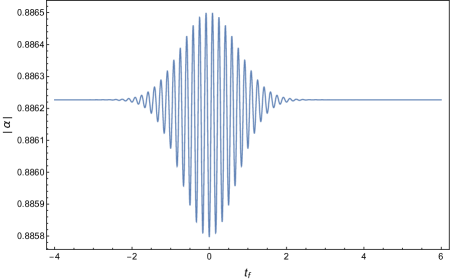
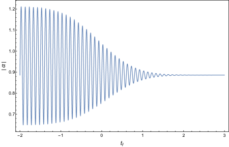
Figure 1: Plot of the magnitude of the displacement $\alpha$ as a function of $t_{f}$, the time lag between the application of the force and the parametric drive. The frequency $\omega(t)$ is assumed to be given by eq (31) and the force $F$ by eq (47). In the upper panel we choose $T_{2}=1$ and $T=0.5,\Omega=1,\omega_{0}=6\pi,\omega_{f}=6\pi$. The lower panel corresponds to the abrupt limit for which we choose $T_{2}=1$ and $\Omega^{2}T=10,\omega_{0}=10\pi,\omega_{f}=10\pi$. In both cases on general grounds we expect to see oscillations for $t_{f}\rightarrow-\infty$ and a constant displacement for $t_{f}\rightarrow\infty$ [see eqs (LABEL:eq:earlyosc) and (20)]. The asymptotic oscillations in the upper panel are suppressed because $B\approx 0$ in this case. In the lower panel the oscillations are observed to turn off smoothly as a function of $t_{f}$, behavior that is also found analytically in the opposite adiabatic limit. In the upper panel by contrast the oscillations turn on only at intermediate times illustrating the remarkable variety of possible behaviors.

3.4 The Adiabatic limit

The adiabatic limit is of particular interest for experimental applications. Our objective is now to solve eq (1) in the limit that $\omega^{2}(t)$ varies slowly. Formally we wish to take the limit $\omega_{0}T\rightarrow\infty$. This is a subtle limit. If we interpret eq (1) with $F=0$ as a Schrödinger equation, the problem we wish to solve is that of reflection above a slowly varying barrier. The conventional WKB approximation fails to capture the effect and yields $B\approx 0$. However by continuation in the complex plane one can obtain the exponentially small value of the scattering coefficient landauqm . For analysis of the forcing one needs not only the scattering coefficients but rather the entire solution $\xi(t)$. Considering its vintage this problem was solved relatively recently berry by a sophisticated use of divergent series.

Applying these techniques here we wish to solve

$$\frac{d^{2}x}{dt^{2}}+\left[\omega_{0}^{2}-\frac{\Omega^{2}}{\cosh^{2}(t/T)}\right]x=0.$$ (48)

Note that we have changed the sign of the term with coefficient $\Omega^{2}$. The adiabatic analysis for the case with this sign is a bit simpler and we focus on this case to avoid unneeded complications. We must assume that $\Omega^{2}<\omega_{0}^{2}$ to ensure that the oscillator remains stable at all times.

The exponentially small corrections to the conventional WKB approximation are controlled by the turning points at which $\omega^{2}(t)=0$. There are no turning points for $t$ real but if we allow complex $t$ there are an infinity of turning points along the imaginary axis. Let $\varphi_{1}$ be the solution to $\cos\varphi=\Omega/\omega_{0}$ that lies in the range $0\leq\varphi_{1}\leq\pi/2$. Then the two turning points closest to the real axis are $t=\pm i\varphi_{1}T$. There is an additional pair of turning points at $t=\pm i\varphi_{2}T$ where $\varphi_{2}$ is the solution to $\cos\varphi=-\Omega/\omega_{0}$ that lies in the range $\pi/2\leq\varphi_{2}\leq\pi$. Finally these four turning points are repeated periodically along the imaginary axis at $t=\pm i\varphi_{1,2}T+2\pi inT$ where $n$ is an integer.

It is useful to rewrite eq (48) along the imaginary axis by making the substitution $t\rightarrow is$. We obtain

$$\frac{d^{2}x}{ds^{2}}+\left[\frac{\Omega^{2}}{\cos^{2}(s/T)}-\omega_{0}^{2}\right]x=0.$$ (49)

The conventional WKB solutions to this equation are real exponentials revealing that in the terminology of berry the segment of the imaginary axis that connects the turning points $\pm i\varphi_{1}T$ is a Stokes line that intersects the real time axis.

It now follows from ref berry that the adiabatic solution to eq (48) with our preferred Jost boundary condition is

$$\xi(t) \approx \sqrt{\frac{\omega_{0}}{\omega(t)}}\left\{\exp\left[-i\int_{0}^{t}d\tau\omega(\tau)\right]\right.$$

$$+ \exp\left.\left[-\omega_{0}Tg\left(\frac{\Omega}{\omega_{0}}\right)\right]U(t)\exp\left[i\int_{0}^{t}d\tau\omega(\tau)\right]\right\}.$$

where $g$ is defined below. The upper line on the right hand side of eq (LABEL:eq:berry) corresponds to the conventional WKB solution. The second line corresponds to the exponentially small backscattering. The coefficient $B$ is given by

$$B\approx\exp\left[-\omega_{0}Tg\left(\frac{\Omega}{\omega_{0}}\right)\right],$$ (51)

while $U(t)$ is a smooth step function that goes from zero to one across the Stokes line with the universal form

$$U(t)={\rm Erf}\left(\frac{t}{T_{S}}\right)\hskip 5.69054pt{\rm with}\hskip 5.69054ptT_{S}=\frac{\omega_{0}Tg(\Omega/\omega_{0})}{2\sqrt{\omega_{0}^{2}-\Omega^{2}}}.$$ (52)

The function $g$ is determined by the integral of $\omega(t)$ along the the Stokes line from the origin to the nearest turning point

$$\omega_{0}Tg\left(\frac{\Omega}{\omega_{0}}\right)=\int_{0}^{\varphi_{1}T}ds\;\sqrt{\omega_{0}^{2}-\frac{\Omega^{2}}{\cos^{2}(s/T)}}=\frac{\pi}{2}(\omega_{0}-\Omega)T.$$ (53)

For illustration consider the displacement produced by a force $F(t)=f(t-t_{f})$ that acts at time $t_{f}$ and has duration $T_{2}$. Assume for simplicity that $|t_{f}|\ll T$ so that the force acts at the same time as the parametric drive and that the force is a brief impulse so that $T_{2}\ll T_{S},T$. In this regime the integrals in eq (16) can be evaluated asymptotically and yield the result

$$\alpha = \frac{ie^{-i\omega_{0}t}}{\sqrt{2m\omega_{{\rm eff}}}}e^{i\omega_{{\rm eff}}t_{f}}\tilde{f}(\omega_{{\rm eff}})$$

$$- \frac{ie^{-i\omega_{0}t}}{\sqrt{2m\omega_{{\rm eff}}}}e^{-i\omega_{{\rm eff}}t_{f}}\tilde{f}^{\ast}(\omega_{{\rm eff}})\exp\left[-\omega_{0}Tg\left(\frac{\Omega}{\omega_{0}}\right)\right]{\rm Erfc}\left(\frac{t}{T_{S}}\right).$$

Here $\omega_{{\rm eff}}=\sqrt{\omega_{0}^{2}-\Omega^{2}}$ and ${\rm Erfc}$ is the complementary error function. Eq (LABEL:eq:adiabaticalpha) reveals that if $|\alpha|$ is plotted as a function of $t_{f}$ there will be oscillations due to the interference between the two terms. Note that the second term is modulated by a complementary error function and vanishes as $t_{f}\rightarrow\infty$. The oscillations likewise vanish as $t_{f}\rightarrow\infty$ with a complementary error function profile.

4 Conclusion

In this paper we study the radiation produced when a field is excited both parametrically and driven by a classical source. Normally in an experiment to measure the dynamical Casimir effect all sources of radiation besides the parametrically excited vacuum radiation are minimized and the field is not driven classically. However our finding that the parametric drive has a strong effect on the radiation field when both kinds of excitation are applied suggests that it may be possible to extract signatures of the quantum effects of the parametric drive even in experiments where classical sources are present.

Cavitation of bubbles in superfluid helium provides a possible realization of this physics. The motion of the bubble wall would parametrically excite phonons in the fluid much as a moving mirror excites photons moore . Moreover, unlike a moving mirror, a moving bubble wall is a strong classical source of acoustic radiation landaufluid . Cavitating bubbles might even be able to achieve supersonic flow putterman leading to the formation of a sound horizon unruh . Although bubbles in superfluid helium are well-studied heliumreview these are likely challenging experiments and it would be desirable in future work to develop an optimum experimental design.

In ref superconduct the dynamical Casimir effect was realized by terminating a transmission line with a SQUID. Changing the flux in the SQUID modifies the boundary condition at the termination effectively mimicking a moving mirror. The flux is varied periodically coupling electromagnetic modes in pairs and leading to the formation of two-mode squeezed states loudonreview . In this case it is feasible to drive the transmission line with a weak classical voltage source. Designing an unambiguous signature of the quantum effects of the parametric drive on the resulting radiation field is therefore an interesting question for future work.

A primary motivation for this work is to develop an estimate of the quantum contribution to gravitational radiation produced by astrophysical phenomena such as black hole mergers that are accessible to LIGO and its planned successor gravitational wave observatories. Mergers are strong classical sources of gravitational radiation and in this case quantum effects, if at all detectable, necessarily have to be observed against this background.

References

- (1) H.B.G. Casimir, “On the attraction between two perfectly conducting plates”, Proc. K. Ned. Akad. Wed. 51, 793 (1948).
- (2) G.T. Moore, “Quantum Theory of the Electromagnetic Field in a Variable-Length One-Dimensional Cavity”, J. Math. Phys 11, 2679 (1970).
- (3) L. Parker, “Quantized Fields and Particle Creation in Expanding Universes”, Phys. Rev. 183, 1057 (1969).
- (4) See, for example, S. Weinberg, Cosmology, Chapter 10 (Cambridge University Press).
- (5) S.W. Hawking “Black hole explosions”, Nature 248, 30 (1974); “Particle Creation by Black Holes”, Commun. Math. Phys. 43, 199 (1975).
- (6) S.K. Lamoreaux, “Demonstration of the Casimir Force in the 0.6 to 6 m Range”, Phys. Rev. Lett. 81, 5475 (1998); U. Mohideen and A. Roy, “Precision Measurement of the Casimir Force from 0.1 to 0.9 m”, Phys. Rev. Lett. 81, 4549 (1998).
- (7) C.M. Wilson et al., “Observation of the dynamical Casimir effect in a superconducting circuit”, Nature 479, 376 (2011).
- (8) W.G. Unruh, “Experimental Black-Hole Evaporation”, Phys. Rev. Lett. 46, 1351 (1981).
- (9) J. Steinhauer, “Observation of quantum Hawking radiation and its entanglement in an analogue black hole”, Nature Physics 12, 959 (2016).
- (10) See, for example, V. Mukhanov and S. Winitzki, Introduction to Quantum Effects in Gravity (Cambridge University Press 2007).
- (11) R.M. Wald, “Stimulated-emission effects in particle creation near black holes”, Phys. Rev. D13, 3176 (1976).
- (12) B.P. Abbott et al., “Observation of Gravitational Waves from a Binary Black Hole Merger”, Phys. Rev. Lett. 116, 061102-061118 (2016).
- (13) F. Pretorius, “Evolution of binary black hole spacetimes”, Phys. Rev. Lett. 95, 121101 (2005); M. Campanelli, C.O. Lousto, P. Marronetti and Y. Zlochower, “Accurate Evolutions of orbiting black-hole binaries without excision”, Phys. Rev. Lett. 96, 111101 (2006); J.G. Baker, J. Centrella, D.-I. Choi, M. Koppitz and J. van Meter, “Gravitational wave extraction from an inspiraling configuration of merging black holes”, Phys. Rev. Lett. 96, 111102 (2006).
- (14) R. Loudon, The Quantum Theory of Light (Oxford University Press 1983).
- (15) M.E. Peskin and D.V. Schroeder, An Introduction to Quantum Field Theory (CRC Press, 2015).
- (16) See for example R. Loudon and P.L. Knight, “Squeezed Light”, Journal of Modern Optics 34, 709 (1987).
- (17) C. Bernard and A. Duncan, “Regularization and Renormalization of Quantum Field Theory in Curved Space-Time”, Annals of Physics 107, 201 (1977); N.D. Birrell and P.C.W. Davies, Quantum fields in curved space, section 3.4 (Cambridge University Press 1984).
- (18) L.D. Landau and E.M. Lifshitz, Course of Theoretical Physics, vol 3, Non-Relativistic Quantum Mechanics, section 23 (Butterworth-Heinemann, 3rd ed, 1981).
- (19) M.V. Berry, “Waves near Stokes Lines”, Proc. Roy. Soc. Lond. A427, 265 (1990).
- (20) L.D. Landau and E.M. Lifshitz, Course of Theoretical Physics, vol 6, Fluid Mechanics, section 73 (Butterworth-Heinemann, 2nd ed, 1987).
- (21) R. Löfstedt, B.P. Barber and S.J. Putterman, “Towards a hydrodynamic theory of sonoluminscence”, Physics of Fluids 5, 2911 (1993); M.P. Brenner, S. Hilgenfeldt and D. Lohse, “Single bubble sonoluminescence”, Rev Mod Phys 74, 425 (2002).
- (22) M. Cole, “Electronic surface states of liquid helium”, Rev. Mod. Phys. 46, 451 (1974).